Available online at www.sciencedirect.com Procedia Chemistry 00 (2014) 000–000 www.elsevier.com/locate/procedia EMERGING TRENDS IN DRUG DISCOVERY - AICADD-2014 Finding hub proteins and their interactions in a Protein-Protein Interaction Network Using GPU P B JAYARAJ a , T SHIJITH a , G GOPAKUMAR a a Department of Computer Science and Engineering, National Institute of Technology Calicut, India Abstract Analysis of proteins, hub proteins and their interactions are important in disease identification and drug target finding of drug discovery process.Markov Clustering algorithm has been effectively used in many bioinformatics applications for analysing large biological networks. A sequential implementation of the MCL algorithm incurs large overheads, in terms of time costs, as the network has a large number of protein nodes and edges. Parallel computing techniques implemented with the help of a GPU can reduce the execution time by operating on various data segments simultaneously. Sequential and parallel implementation of MCL algorithm generates clusters with low granularity. But due to the scale-free nature of the Protein-Protein Interaction network, flows simulated in MCL by random walks fail to capture the actual picture of granulated clusters. In order to address this problem with MCL, we propose to introduce a fast parallel method, in which we pre-process the input data to reduce its uneven density and thus effectively randomising the network. The convergence of the higher degree node sets to a single node need to be approximated in this method and to balance this convergence effect, some weight adjustment steps are introduced in the input stochastic matrix. After MCL is processed, the converged nodes in the resultant network will be replaced by their original node sets. This method ensures better clustering with more interacting edges. A variant of the above mentioned method with no weight adjustment step further captures the presence of inter connected links between the dense regions in the network. Since the pre-processing step removes the dense regions in the graph, the low flow inter connected edges between the dense regions gets more priority in the MCL process. Hence we have obtained an improved cluster granularity with our new method by boosting the clustering coefficient from 0.04 to 0.22. Our modified method also sheds more light on the linkages between the various dense regions in the network. Nearly 4-5X improvement in execution speed was reported when new methods were implemented. We have used NVIDIA CUDA enabled GPU architecture for implementation purposes. c 2014 The Authors. Published by Elsevier B.V. Peer-review under responsibility of scientific committee of AICADD-2014. Keywords: Protein–Protein Interaction Networks ; Markov Clustering; GPU Computing; Graphs; Networks; CUDA; Parallel Programming; 1. Introduction Proteins are biological molecules consisting of one or more amino acid chains. They perform various functions within living organisms, including catalyzing metabolic reactions, replicating DNA, responding to stimuli, giving structure to biological components, and transporting molecules from one location to another. To achieve these func- tions they interact among themselves and with other molecules in the body. Therefore, the study of protein interactions is very crucial for the understanding of cell behaviour, protein complexes and pathways. A Protein-Protein Interaction Network (PPIN) is the graph obtained by representing proteins as nodes and their interactions with other proteins as edges 1,2 . Usually, these networks contain hundreds of proteins and their interactions and analysing these networks 1876-6196 c 2014 The Authors. Published by Elsevier B.V. Peer-review under responsibility of scientific committee of AICADD-2014.
Proteins are biological molecules consisting of one or more amino acid chains. They perform various functionswithin living organisms, including catalyzing metabolic reactions, replicating DNA, responding to stimuli, givingstructure to biological components, and transporting molecules from one location to another. To achieve these func-tions they interact among themselves and with other molecules in the body. Therefore, the study of protein interactionsis very crucial for the understanding of cell behaviour, protein complexes and pathways. A Protein-Protein InteractionNetwork (PPIN) is the graph obtained by representing proteins as nodes and their interactions with other proteins asedges1,2. Usually, these networks contain hundreds of proteins and their interactions and analysing these networks
2 P. B. Jayaraj et al. / Procedia Chemistry 00 (2014) 000–000
require efficient computational methods to extract useful information. Clustering is one such useful tool. Using clus-tering algorithms, proteins can be grouped into various partitions according to their degree of interactions with eachother. In this study, Markov Clustering algorithm (MCL) is the clustering technique used to cluster information fromthe PPI network.
A PPI network is scale-free since its node degree follows power-law distribution. So the topological structure ofPPI network has a lot of interconnected dense regions. Each dense region could be a functional module or a proteincomplex3. Essential proteins in the PPI network are called hub proteins and they will have high degree4,5. So hubproteins can be found in dense regions. Any change in a hub protein creates some malfunction and can lead to adisease whereas change in the interacting partners of hubs has little impact on the network. The other importantcomponent of the network is interconnecting proteins among dense regions. To unearth details like above, one hasto mine the graph deeply. Markov Clustering, a general graph clustering algorithm6,7,8, has been widely used forthe network analysis. MCL involves computationally intensive tasks and thus, implementing MCL on a CPU usingsequential programming methods will fail to produce results within a reasonable time frame due to the large size of thenetwork. The high parallelism expressed by MCL clustering lead to the idea of using parallel computing techniquesto tackle the complexity of the same9. GPU computing technique, which provides a large level of parallelism usinga fraction of the budget required by usual MIMD cluster architectures, can be considered for this implementation.Designed with a massive number of floating point units and very high memory bandwidth, GPUs are widely used inscientific computing to speed up simulation, modelling, visualization, and data analysis. In effect, it gives far greaterprocessing speeds by enabling many more threads to spawn simultaneously. Since the GPU programming paradigmsubstantially differs from the traditional CPU-based computing, algorithms specific to GPU have to be developed, andthis is usually a difficult and tedious process.
When implemented, MCL gave us clusters with weakly interacting links in each cluster. The weakness in theclustering is because MCL uses random walks for cluster partitioning, and this being relatively ineffective for a scale-free network such as a PPI network results in low granularity. We analysed MCL algorithm to work around the abovelimitation. To address this issue, we developed two new methods that retain the strength of MCL while rectifying itsweakness, in this context. In the first method, the clusters will be in the form of dense regions surrounding hubs whileclusters formed using the second method will have multiple dense regions from which we can identify interconnectingedges. The first method finds application in the determination of new functional modules whereas the second methodcan be used in pathway analysis of disease detection and target identification of drug discovery process. Hence theimplementation of the above methods imparts therapeutic value as well.
The paper is divided into 6 sections: Section 2 describes GPU and its architecture. Section 3 gives backgroundinformation about CUDA framework, significance of clustering and MCL algorithm. Section 4 describes two newMCL based parallel clustering methods in detail. Section 5 deals with the Experimental setup, Dataset and discussionsof the result obtained. Conclusions and future scope are described in Section 6.
2. GPUs for Accelerating HPC Workloads
A GPU is a special purpose processor designed to accelerate the computation of graphic operations. The technicaldefinition of GPU10 is a single chip processor with integrated transform, lighting, triangle setup/clipping, and render-ing engines that is capable of processing a minimum of 10 million polygons per second. The design of a GPU is veryspecial that most of their silicon is utilized to perform arithmetic computations11. With the advent of the GPU, com-putationally intensive graphic operations were off loaded from the CPU to the GPU, thus allowing for faster graphicsprocessing speeds12,13,14.
In this paper we focus on the NVIDIA CUDA GPU architecture, as it is the most widely used architecture for GPUcomputing, to parallelise the computationally intensive Markov Clustering method.
The peak performance of the some of the GPU cards (from NVIDIA) that we have used in this work is shownbelow10:
P. B. Jayaraj et al. / Procedia Chemistry 00 (2014) 000–000 3
With power consumption and heat dissipation issues pushing multi-core CPUs to the limit, GPU accelerated com-puting systems have drawn the attention of researchers because they have tremendous computational power and highmemory bandwidth, and are inherently well suited for massively data parallel computation. The latest top 500list of the world’s fastest supercomputers included nearly 50 supercomputers powered by NVIDIA GPUs, and theworld’s second fastest supercomputer, Oak Ridge National Laboratory’s TITAN, utilizes over 18,000 NVIDIA KeplerGPUs15,16. Hence the computing power of the recent GPUs is comparable to the computing power of a cluster withhundreds of CPUs.
3. Background Work
3.1. CUDA
CUDA (Compute Unified Device Architecture) is a parallel computing platform and programming model devel-oped by NVIDIA. It enables dramatic increase in computing performance by harnessing the power of the graphicsprocessing unit (GPU)17. CUDA enabled GPUs are organized in multiprocessors, which group multiple streamingprocessors (SMP), as the basic execution units. CUDA executes the same program on all the multiprocessors. Thecode for the program the kernel is the same but both the data and execution flow can be different. It can launch mul-tiple instances of the kernel called threads. These threads are grouped into warps for execution on a multiprocessor.Hence all threads in a warp will be executed by one multiprocessor in a SIMD manner. The thread managementoverhead is very low in this case, since the threads are created and scheduled by the hardware itself and intermediarysoftware is not involved. All architecture details, threads, warps, and multiprocessors are hidden from the end user;CUDA instead introduces the notion of threads, blocks and grids to ease the decomposition of the problem domain.In short, threads are both the physical and logical unit of execution; the GPU groups and schedules threads in warps,while CUDA offers a higher level view of grids and blocks. Grids and blocks can be used by the programmer to mapthe subdivisions inherent in the problem domain in a convenient way18. Each thread is then provided with variablesrepresenting the block and grid co-ordinates on which it needs to operate; using these co-ordinates, a thread can accessand process a single item or subset of the problem domain.
A CUDA program consists of one or more phases that are executed either on the host (CPU) or a device such as aGPU19,20,18. The phases that exhibit little or no data parallelism are implemented in host code. The phases that exhibitrich amount of data parallelism are implemented in the device code.
3.2. MCL
Markov Cluster (MCL) is a cluster algorithm for graphs based on the simulation of flow in networks. The crux ofthe algorithm lies in the fact that the number of higher length paths and thus the flow between two arbitrary nodeswithin a dense region is greater than that between two different dense regions. This property implies that the nodesencountered during a random walk on the graph will seldom be from different clusters.
MCL is mainly composed of two processes namely expansion and inflation. The former causes flow to dissipatewithin clusters and coincide with taking the power of a stochastic matrix whereas the latter eliminates flow betweendifferent clusters. These two are alternated until the matrix they operate on becomes idempotent21.
EXPm(P) = Pm (1)
The algorithm uses a stochastic process called Markov chain which consists of a finite number of states and prob-abilities pi j which denotes the transition probability or probability of moving from state j to i. If this happens with
4 P. B. Jayaraj et al. / Procedia Chemistry 00 (2014) 000–000
m − 1 states in between i and j, it is called m-step transition probability and is denoted by p(m)i j . It is calculated by
summing up the probabilities of all possible paths between i and j in m steps. A matrix P constructed using theseprobability values is called a transition probability matrix. Here, the nodes of the graph are the Markov states and theedge weights correspond to the transition probabilities.
p(m)i j =
∑r
p(m−k)ir p(k)
r j (2)
When we write equation(2) in Matrix form,
P(m) = P(m−k)P(k) (3)
Now substitute m = k-1 in equation(3), it becomes
P(m) = P · P(m−1) (4)
From equation (4), we can also write
P(m−1) = P · P(m−2)
Proceeding, we’ll reachP(m) = P · P · P · · · P = Pm (5)
Inflation operation:
(Γr M)pq = (Mpq)r/
m∑i=1
(Miq)r; i = 1...m; q = 1...n. (6)
where M is a matrix and r > 1 is a real number.The inflation operator can be altered by a parameter r, which is directly proportional to the granularity of clusters.
This process involves taking the rth power of every entry in the matrix followed by a normalization step such thatthe resultant is a column stochastic matrix. Repeated inflation boosts the entries which have high magnitude therebypromoting more probable walks and demotes values which are very small. Inflation is followed by a process calledPrune which discards values that are below a threshold value.
Algorithm 1 MCL
A := A + ∆ // Add self-loops to the graphM := AD−1 // Initialize M as the canonical transition matrixrepeat
M := Mexp := Expand(M)M := Min f := In f late(M, r)M := Prune(M)
until M Converges
Interpret M as a clustering
MCL creates high probability edges within every cluster and a few low probability edges among clusters. Thesenewly formed edges further constraints the flow within the cluster. After inflation, a prune step can be applied toremove values which are less than a particular threshold value. The process stops when matrix becomes idempotentunder expansion and inflation. Input of MCL can be adjacency or weighted matrix of the graph and output is a matrixwhose rows represent clusters.
Need for parallelising MCL: For a graph with n nodes, execution of serial MCL method will take O(n3) as matrixmultiplication plays a major role in the expansion step. Therefore, sequential execution will take a lot of time toproduce result for large values of n. One solution to improve performance is to adopt parallel programming techniques.With parallel programming, multiple independent portions of the input data can be processed simultaneously22. Usingthis, Matrix multiplication can be done in O(n) by parallel execution7,9,23. Current low cost GPU cards loaded with
P. B. Jayaraj et al. / Procedia Chemistry 00 (2014) 000–000 5
thousands of parallel cores can be utilized for computing in parallel since the clustering application is highly dataparallel.
Limitation of MCL: Serial and parallel MCL implementations gave us clusters with weak interacting links in eachcluster. The weakness in the clustering is because MCL uses random walks for cluster partitioning, and this beingrelatively ineffective for a scale-free network such as a PPI network results in low granularity.
4. Proposed methods
In order to rectify the inherent scale-free structure of the PPI network and to correctly identify interactions amongdense regions, a new method has been proposed in this study. This method pre-processes the input network to reduceits uneven density before applying MCL to get an accurate output. It is effective because it uses the underlying denseregions of the pre-processed network to form clusters which can then be used to generate the required output. Thismethod produces clusters with better granularity and size, while a modified version of the above method, with noweight adjustment step, can lucidly identify the interactions among dense regions.
4.1. Method
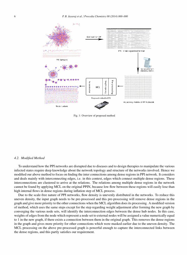
We start identifying inherently dense regions of the given network (node sets of high degree nodes - known as hubs- and their connected neighbours). In a usual PPI network, nodes with degrees higher than 3 are considered hubs. Anew graph is formed by replacing the identified node sets with a new node. Simply stated, node sets converge to asingle node in the new graph. Every node in this new graph will be given a new ID. Edges are created in the newgraph by considering the edge structure of the original PPI network. New edges will be created between two nodesin the new graph, if their corresponding nodes in the original graph are connected. Since a node in the new graph canbe a node set of the original PPI network, an edge will be formed in the new graph from this converged node to allthe neighbours of connected nodes in the original node set. All edge weights are set as equal to 1 if edges exist in theoriginal node set and 0 otherwise. To cancel the effect of convergence, edge weights in new graph from convergednode to its neighbours is approximately adjusted. For example, if there are n nodes in the node set excluding thecentral hub and ’m’ neighbours, a weight of m/n is added to every edge from the converged node. The value of m/nis derived from the Markov equation for finding transition probability. From equation (3), the maximum value oftransition probability between a hub and another node through these ’n’ intermediate nodes will be n (1*1 + 1*1 + ...n times => n). Since these n nodes are not taken into account while calculating probability in new graph, a weightof m/n is added to each of the m edges of the converged node. Now, the transition probability with these m nodes asintermediate nodes will be m * (n/m + 1) => n + m. So the effective loss of probability by way of node convergencecan be compensated. In a real case scenario, the loss of probability will always be less than n. The relatively highprobability hence obtained increases the cluster granularity and its size. Now, the MCL algorithm can be applied onthis pre-processed graph. Algorithm 2 illustrates the pseudo code for the method. The clusters obtained after theMCL process will not contain the actual nodes of original PPI network because of the process of node convergenceand hence these converged nodes have to be replaced with their original node sets. The final clusters obtained willhave more interacting nodes because of the pre-processing (the node convergence and weight adjustments) mechanismwhich acts on the original graph. The figure 1 gives an overview of the working of this method when applied to a PPInetwork
Algorithm 2 Proposed Method
1: mark valid nodes to converge in G2: store mapping of nodes in Map3: create a new graph G’ using Map4: adjust edge weights in G’5: apply MCL on G’6: reconstruct G from G’
6 P. B. Jayaraj et al. / Procedia Chemistry 00 (2014) 000–000
Fig. 1: Overview of proposed method
4.2. Modified Method
To understand how the PPI networks are disrupted due to diseases and to design therapies to manipulate the variousinfected states require deep knowledge about the network topology and structure of the networks involved. Hence wemodified our above method to focus on finding the inter connections among dense regions in PPI network. It considersand deals mainly with interconnecting edges, i.e. in this context, edges which connect multiple dense regions. Theseinterconnections are clustered to arrive at the relations. The relations among multiple dense regions in the networkcannot be found by applying MCL on the original PPIN, because low flow between these regions will easily lose thanhigh internal flows in dense regions during inflation step of MCL process.
Due to the scale-free nature of PPI networks, flow density is unevenly distributed in the networks. To reduce thisuneven density, the input graph needs to be pre-processed and this pre-processing will remove dense regions in thegraph and give more priority to the other connections when the MCL algorithm does its processing. A modified versionof method, which uses the same steps except for the step regarding weight adjustment after forming the new graph byconverging the various node sets, will identify the interconnection edges between the dense hub nodes. In this case,weights of edges from the node which represent a node set to external nodes will be assigned a value numerically equalto 1 in the new graph, if there exists a connection between them in the original graph. This removes the dense regionsin the graph and gives more priority for other connections which were masked earlier due to the uneven density. TheMCL processing on the above pre-processed graph is powerful enough to capture the interconnected links betweenthe dense regions, and this partly satisfies our requirement.
P. B. Jayaraj et al. / Procedia Chemistry 00 (2014) 000–000 7
5. Implementation, Results & Discussion
5.1. Experimental setup
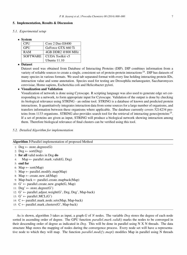
• SystemCPU Core 2 Duo E8400GPU GeForce GTX 660 TiRAM 4GB DDR2 @800 MHzSOFTWARE CUDA Toolkit v5
Ubuntu 11.10• Dataset
Dataset used was obtained from Database of Interacting Proteins (DIP). DIP combines information from avariety of reliable sources to create a single, consistent set of protein-protein interactions24. DIP has datasets ofmany species in various formats. We used tab separated format with every line holding interacting protein IDs,interaction value and some annotation. Species used for testing are Drosophila melanogaster, Saccharomycescerevisiae, Homo sapiens, Escherichia coli and Helicobacter pylori.
• Visualization and ValidationVisualization of network is done using Cytoscape. R scripting language was also used to generate edge set cor-responding to a network, to form appropriate input for Cytoscape. Validation of the output is done by checkingits biological relevance using STRING - an online tool. STRING is a database of known and predicted proteininteractions. It quantitatively integrates interaction data from some sources for a large number of organisms, andtransfers information between these organisms where applicable. The database currently covers 5214234 pro-teins from 1133 organisms. STRING also provides search tool for the retrieval of interacting genes/proteins25.If a set of proteins are given as input, STRING will produce a biological network showing interaction amongthem. Therefore biological relevance of final clusters can be verified using this tool.
5.2. Detailed Algorithm for implementation
Algorithm 3 Parallel implementation of proposed Method
1: Deg← store degrees(G)2: Deg← sort(Deg)3: for all valid nodes in Deg do4: Map← parallel mark valid(G, Deg)5: end for6: Map← sort(Map)7: Map← parallel modify map(Map)8: Map← create new id(Map)9: Map-back← parallel create mapback(Map)
10: G’← parallel create new graph(G, Map)11: Deg’← store degree(G’)12: G’← parallel adjust weight(G’, Deg, Deg’, Map-back)13: G’← parallel MCL(G’)14: C← parallel mark node sets(Map, Map-back)15: C← parallel mark clusters(G’, Map-back)
As is shown, algorithm 3 takes as input, a graph G of N nodes. The variable Deg stores the degree of each nodesorted in ascending order of degree. The GPU function parallel mark valid() marks the nodes to be converged intheir descending order of degree as indicated in Deg. This will be done in parallel using N X N threads. The datastructure Map stores the mapping of nodes during the convergence process. Every node set will have a representa-tive node to which they will map. The function parallel modi f y map() modifies Map in parallel using N threads
8 P. B. Jayaraj et al. / Procedia Chemistry 00 (2014) 000–000
while parallel create mapback() stores the relation between new nodes and old to reconstruct graph after clusteringin Map-back. In Map-back, a new node representing a node set will be related to its representative node. Graph G′
is constructed from Graph G with new nodes and their relation with original nodes present in Map. The functionparallel create new graph() does the same in constant time using N x N threads. Deg’ is a data structure whichstores the degree of all nodes in graph G′. The function parallel ad just weight() executes weight adjustment andworks in constant time by spawning N X N threads. GPU kernel parallel MCL() ensures parallel implementation ofMarkov clustering on input Graph G. The expansion step of MCL which involves matrix multiplication will entail acomplexity of O(n) by N X N parallel thread creation (but the actual hardware is finite in real). The inflation processof MCL, on the other hand, which involves squaring, summing and normalizing operations will execute in constanttime by separate N x N threads. Kernel functions parallel mark node sets() and parallel mark clusters() recreatethe final cluster in G′ to represent the original nodes of G. Both functions execute in constant time simultaneouslyusing N, N X N threads respectively. The data set C is harnessed to store the final clusters obtained after the operationson input graph G.
The source of code and other details of the present implementation can be found at:http://andromeda.nitc.ac.in/jayarajpb/link1.php?pname= GPU%20based%20Fast%20PPI%20Clustering
5.3. Result
Our experiments resulted in lesser execution time with the proposed methods when compared to MCL because ofthe pre-processing step, i.e., converging dense regions to reduce the input graph size, that we adopted. Table 1 showsthis improvement in execution time for various input datasets considered. That means, improvement in executiontime may depend upon the topology of the input network. As the size of PPIN increases, it incorporates more denseregions and the correspnding improvement in execution time may be significant. Other than the improvement inexecution time, the granularity of clusters formed by our first method is also higher than that of MCL due to theweight adjustment process adopted after the converging step. This resulted in better clustering results when comparedwith MCL on PPIN. Average clustering coefficients of 0.04 and 0.22 were obtained when MCL and proposed methodwere applied on PPIN of Saccharomyces cerevisiae respectively. Additionally, average cluster size for our proposedmethod was increased from 15.62 to 16.9 and produced 50 less clusters than applying MCL alone.
Table 1: Comparison of execution time of proposed method and MCL on PPINs of various organisms
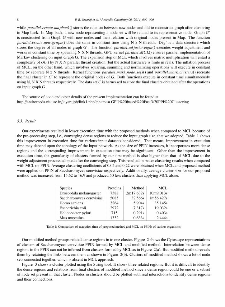
Our modified method groups related dense regions in to one cluster. Figure 2 shows the Cytoscape representationsof clusters of Saccharomyces cerevisiae PPIN formed by MCL and modified method. Interrelation between denseregions in the PPIN can not be inferred from clusters formed by MCL as in Figure 2(a). But modified method revealsthem by retaining the links between them as shown in Figure 2(b). Clusters of modified method shows a lot of nodesets connected together, which is absent in MCL approach.
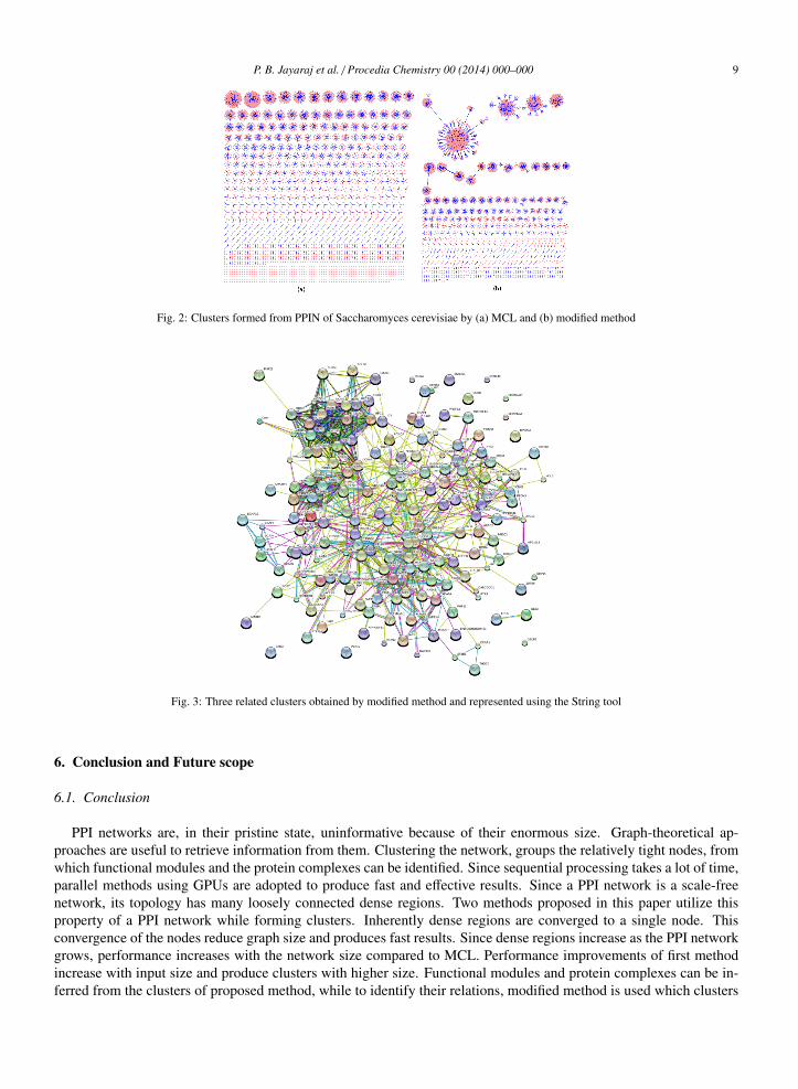
Figure 3 shows a cluster plotted using the String tool. It shows three related regions. But it is difficult to identifythe dense regions and relations from final clusters of modified method since a dense region could be one or a subsetof node set present in that cluster. Nodes in clusters should be plotted with real interactions to identify dense regionsand their connections.
P. B. Jayaraj et al. / Procedia Chemistry 00 (2014) 000–000 9
Fig. 2: Clusters formed from PPIN of Saccharomyces cerevisiae by (a) MCL and (b) modified method
Fig. 3: Three related clusters obtained by modified method and represented using the String tool
6. Conclusion and Future scope
6.1. Conclusion
PPI networks are, in their pristine state, uninformative because of their enormous size. Graph-theoretical ap-proaches are useful to retrieve information from them. Clustering the network, groups the relatively tight nodes, fromwhich functional modules and the protein complexes can be identified. Since sequential processing takes a lot of time,parallel methods using GPUs are adopted to produce fast and effective results. Since a PPI network is a scale-freenetwork, its topology has many loosely connected dense regions. Two methods proposed in this paper utilize thisproperty of a PPI network while forming clusters. Inherently dense regions are converged to a single node. Thisconvergence of the nodes reduce graph size and produces fast results. Since dense regions increase as the PPI networkgrows, performance increases with the network size compared to MCL. Performance improvements of first methodincrease with input size and produce clusters with higher size. Functional modules and protein complexes can be in-ferred from the clusters of proposed method, while to identify their relations, modified method is used which clusters
10 P. B. Jayaraj et al. / Procedia Chemistry 00 (2014) 000–000
nodes based on the interconnection of inherently dense regions in the network. Hence these methods use different andnew approaches to analyze a PPI network.
6.2. Future scope
Our modified method can be used to find biological pathways of a network, since they connects multiple denseregions. These methods can be used to process other scale free networks also. Social networks, Internet, biologicalnetworks are examples of scale-free network.
6.3. Future work
Due to the huge size of the network, memory will be the bottleneck in GPU. Geforce NVIDIA graphics cardgenerally carries only 1 to 2 GB graphics RAM. As the current network size goes beyond the above limit, onehas to use sparse matrix representations for the graph, which will in turn reduce the memory use because of thehigh sparseness of scale-free network. ELLPACK-R is a good storage technique for this implementation. Since anapproximation technique is applied in pre-processing step, the degree of approximation error has to be found bycomparing the new method with regular serial MCL.
Also disease and non-disease datasets of an organism can be analyzed in order to identify irregularities in networkswhich would essentially enable a biologist to easily predict a disease in the human body.
6.4. ACKNOWLEDGEMENT
We thank the Computer Science and Engineering Department of NIT Calicut for all the support provided towardsthe successful completion of this work.
References
1. K. Raman, “Construction and analysis of protein-protein interaction networks,” Automated Experimentation, vol. 2, no. 1, pp. 2+, 2010.2. A. Rao, G. Bulusu, R. Srinivasan, and T. Joseph, “Protein-Protein Interactions and Disease,” Protein Interactions, 2012. [Online]. Available:
http://www.intechopen.com/books/protein-interactions/protein-protein-interactions-and-disease3. V. Spirin and L. A. Mirny, “Protein complexes and functional modules in molecular networks,” Proceedings of the National Academy of
Sciences, vol. 100, no. 21, pp. 12 123–12 128, Oct. 2003. [Online]. Available: http://dx.doi.org/10.1073/pnas.20323241004. R. R. Vallabhajosyula, D. Chakravarti, S. Lutfeali, A. Ray, and A. Raval, “Identifying hubs in protein interaction networks,” PLoS ONE,
vol. 4, no. 4, p. e5344, 04 2009. [Online]. Available: http://dx.doi.org/10.13712Fjournal.pone.00053445. X. He and J. Zhang, “Why do hubs tend to be essential in protein networks?” PLoS Genet, vol. 2, no. 6, p. e88, 06 2006.6. A. J. Enright, S. Van Dongen, and C. A. Ouzounis, “An efficient algorithm for large-scale detection of protein families,” Nucleic Acids
Research, vol. 30, no. 7, pp. 1575–1584, Apr 2002.7. S. Brohe and J. van Helden, “Evaluation of clustering algorithms for protein-protein interaction networks,” BMC Bioinformatics, vol. 7, pp.
1–19, 2006. [Online]. Available: http://dx.doi.org/10.1186/1471-2105-7-4888. C. Lin, Y.-R. Cho, W.-C. Hwang, P. Pei, and A. Zhang, Clustering Methods in a ProteinProtein Interaction Network. John Wiley & Sons,
Inc., 2007, pp. 319–355. [Online]. Available: http://dx.doi.org/10.1002/9780470124642.ch169. A. Bustamam, K. Burrage, and N. Hamilton, “Fast parallel markov clustering in bioinformatics using massively parallel computing on gpu
with cuda and ellpack-r sparse format,” Computational Biology and Bioinformatics, IEEE/ACM Transactions on, vol. 9, no. 3, pp. 679 –692,May-June 2012.
10. NVIDIA, “Cuda developer website to provide resources.” https://developer.nvidia.com/category/zone/cuda-zone, Jun. 2013.11. NVIDIA Corporation, “NVIDIA CUDA C programming guide,” 2011, version 4.1.12. D. Luebke and G. Humphreys, “How gpus work,” Computer, vol. 40, no. 2, pp. 96–100, 2007.13. S. Keckler, W. Dally, B. Khailany, M. Garland, and D. Glasco, “Gpus and the future of parallel computing,” Micro, IEEE, vol. 31, no. 5, pp.
7–17, 2011.14. C. McClanahan, “History and evolution of gpu architecture,” http://mcclanahoochie.com/blog/wp-content/uploads/2011/03/gpu-hist-
paper.pdf, Jun. 2013.15. Fermi Architecture White Paper - Nvidia., 1st ed., NVIDIA Corporation., 2009. [Online]. Available:
http://www.nvidia.in/content/PDF/kepler/NVIDIA-Kepler-GK110-Architecture-Whitepaper.pdf17. D. B. Kirk and W. mei W. Hwu, Programming Massively Parallel Processors - A Hands-on Approach. Morgan Kaufmann, 2010.18. L. Dematt and D. Prandi, “Gpu computing for systems biology,” Briefings in Bioinformatics, vol. 11, no. 3, pp. 323–333, 2010. [Online].
P. B. Jayaraj et al. / Procedia Chemistry 00 (2014) 000–000 11
19. J. Sanders and E. Kandrot, CUDA by Example: An Introduction to General-Purpose GPU Programming, 1st ed. Addison-WesleyProfessional, Jul. 2010. [Online]. Available: http://www.amazon.com/exec/obidos/redirect?tag=citeulike07-20&path=ASIN/0131387685
20. CUDA C Best Practices Guide, 4th ed., NVIDIA Corporation, 2701 San Tomas Expressway, Santa Clara 95050, USA, May 2011. [Online].Available: http://developer.download.nvidia.com/compute/DevZone/docs/html/ C/doc/CUDA C Best Practices Guide.pdf
21. S. Van Dongen, “Graph clustering via a discrete uncoupling process,” SIAM J. Matrix Anal. Appl., vol. 30, no. 1, pp. 121–141, Feb. 2008.[Online]. Available: http://dx.doi.org/10.1137/040608635
22. O. Trelles, “On the parallelisation of bioinformatics applications,” Briefings in Bioinformatics, vol. 2, no. 2, pp. 181–194, 2001. [Online].Available: http://bib.oxfordjournals.org/content/2/2/181.abstract
23. N. Bell and M. Garland, “Efficient sparse matrix-vector multiplication on CUDA,” NVIDIA Corporation, NVIDIA Technical Report NVR-2008-004, Dec. 2008.
24. Database of Interacting Proteins, “http://dip.doe-mbi.ucla.edu/dip/main.cgi,” February 2013.25. STRING is a database of known and predicted PPI, “http://string-db.org/,” February 2013.