Emission Trading Systems and the Optimal Technology Mix * Gregor Zoettl † University of Munich April 12, 2011 Abstract Cap and trade mechanisms enjoy increasing importance in environmental legis- lation worldwide. The most prominent example is given by the European Union Emission Trading System (EU ETS) designed to limit emissions of greenhouse gases, several other countries already have or are planning the introduction of such systems. One of the important aspects of designing cap and trade mechanisms is the possibil- ity of competition authorities to grant emission permits for free. Free allocation of permits which is based on past output or past emissions can lead to inefficient produc- tion decisions of firms (compare for example B¨ohringer and Lange (2005), Rosendahl (2007), Mackenzie et al. (2008), Harstad and Eskeland (2010)). Current cap and trade systems often grant free allocations based on installed production facilities, however. Different technologies receive different levels of free allocations 1 , this has a direct impact on the technology mix chosen by firms. It is the purpose of the present article to study the impact of a cap and trade mechanism not only on firms’ output decisions but also on their investment incentives in different technologies and to analyze the optimal design of emission trading systems in such an environment. Keywords: Emissions Trading, Free Allocation, Investment Incentives, Technology Mix. JEL classification: H21, H23, Q55, Q58, 033 * We want to thank Veronika Grimm, Karsten Neuhoff and Yves Smeers for many valuable comments. † University of Munich, Dep. of Economics, Ludwigstrasse 28, Munich, Germany, [email protected]. 1 See the present phase II of the EU ETS, for example German Parliament (2007) for the case of Germany. 1
Transcript
Emission Trading Systems and the Optimal Technology
Mix ∗
Gregor Zoettl†
University of Munich
April 12, 2011
Abstract
Cap and trade mechanisms enjoy increasing importance in environmental legis-
lation worldwide. The most prominent example is given by the European Union
Emission Trading System (EU ETS) designed to limit emissions of greenhouse gases,
several other countries already have or are planning the introduction of such systems.
One of the important aspects of designing cap and trade mechanisms is the possibil-
ity of competition authorities to grant emission permits for free. Free allocation of
permits which is based on past output or past emissions can lead to inefficient produc-
tion decisions of firms (compare for example Bohringer and Lange (2005), Rosendahl
(2007), Mackenzie et al. (2008), Harstad and Eskeland (2010)).
Current cap and trade systems often grant free allocations based on installed
production facilities, however. Different technologies receive different levels of free
allocations1, this has a direct impact on the technology mix chosen by firms. It is
the purpose of the present article to study the impact of a cap and trade mechanism
not only on firms’ output decisions but also on their investment incentives in different
technologies and to analyze the optimal design of emission trading systems in such
∗We want to thank Veronika Grimm, Karsten Neuhoff and Yves Smeers for many valuable comments.†University of Munich, Dep. of Economics, Ludwigstrasse 28, Munich, Germany, [email protected] the present phase II of the EU ETS, for example German Parliament (2007) for the case of Germany.
1
1 Introduction
In the present article we analyze cap and trade mechanisms which grant technology specific
free allocations.1 We determine the impact of such mechanisms both on firms’ investment
decisions in different technologies and on their final production decisions. We then derive
the optimal design of such a mechanism for ideal market conditions but also for non-ideal
situations where firms either exercise market power or competition authorities’ decisions
are partially constrained by requirements of political or legislative processes.
Cap and trade mechanisms designed to internalize social cost of pollution enjoy increas-
ing importance in environmental legislation worldwide. A prominent example is given by
the European Union Emission Trading System (EU ETS), several other countries already
have or are planning the introduction of such systems.2 An important aspect when in-
troducing cap and trade mechanisms is the possibility of competition authorities to grant
emission permits for free. This apparently allowed to crucially facilitate the political pro-
cesses which finally lead to the introduction of currently adopted cap and trade systems.
As Convery(2009) in a recent survey on the origins and the development of the EU ETS
observes:“The key quid pro quos to secure industry support in Germany and across the
EU were agreements that allocation would take place at Member State level [...], and that
the allowances would be free”. Very similar observations can also be found in many other
contributions to that issue.3
A one and for all lump sum allocation of permits, which is entirely independent of firms’
actions has a purely distributive impact in case firms take the market price of emission
permits as given. This fundamental insight in principle dates back to Coase (1960). Recent
contributions which apply those findings to the case of firms’ incentives to adopt cleaner
technologies include for example Requate and Unnold (2001), Montero (2002), or Requate
and Unnold (2003), for a survey of this literature compare Requate (2005). 4
2Those include New Zealand, Australia, Canada, United States, for an overview See IEA (2010).3As for example Tietenberg (2006) observes: ”free distribution of permits (as opposed to auctioning
them off) seems to be a key ingredient in the successful implementation of emissions trading programs”.
Bovenberg et al. (2008) state:“The compensation issue has come to the fore in recent policy discussions.
For example, several climate change policy bills recently introduced in the U.S. Congress (for example, one
by Senator Jeff Bingaman of New Mexico and another by Senator Dianne Feinstein of California) contain
very specific language stating that affected energy companies should receive just enough compensation to
prevent their equity values from falling.”4This independence result no longer holds if firms are aware that their actions have an impact on
the equilibrium permit price then this equivalence breaks down. Compare for example Monteiro (2002) or
Hintermann (2011) which analyze strategic behavior at the permit markets. For a survey of the “conditions
under which the independence property is likely to hold both in theory and in practice”, see Hahn and
Stavis (2010).
2
The design of free allocations in currently active cap and trade systems is not very likely
to have such lump sum property but will include explicit or implicit features of updating,
as several authors argue. Compare for example Neuhoff et al. (2006) who observe for the
case of the EU ETS: “For the phase I trading period, incumbent firms received allowances
based on their historic emissions.[...] For future trading periods, the Member States have
to again define NAPs for the ETS. [...] It is likely that the base period will be adjusted over
time to reflect changes in the distribution of plants over time. It is, for example, difficult to
envisage that in phase II a government will decide to allocate allowances to a power plant
that closed down in phase I. This suggests that some element of ’updating’ of allocation
plans cannot be avoided if such plans are made sequentially.”
Updating of free allocation schemes designed to consistently adapt to an industry’s
dynamic development has an impact on firms’ behavior, however. First, it leads to a
distortion of the operation of existing production facilities if firms believe that current
output or emissions do have an impact on allocations granted to those facilities in the
future.5 Second, it has an impact on firms’ incentives to modify their production facilities
through upgrading, retiring and building of new facilities if free and technology specific
allocations are granted contingent on installed facilities. The literature which analyzes
the impact of updating on firms’ behavior up to now has focused on the first aspect.
That is, those contributions provide very rich insight on the impact of updating based
on past output or emissions on firms’ production and emission decisions, they abstract
from changed free allocations to a firm due to changed installed facilities, however. The
most prominent contributions include Moledina et al. (2003), Bohringer and Lange (2005),
Rosendahl(2007), Mackenzie et al. (2008), or Harstadt and Eskeland (2010).6
A recent review by the International Energy Agency (IEA 2010) of all current and
planned emission trading schemes worldwide reveals, however that most legislations which
provide free emission permits do indeed update based on currently installed production
facilities.7 The precise design of free allocations thus clearly has an impact on firms’ in-
5Compare for example Bohringer and Lange (2005):“As a case in point, one major policy concern is
that [...] the allocation should account for (major) changes in the activity level of firms. Free allocation
schemes must then abstain from lump-sum transfers and revert to output- or emission-based allocation.”6In a recent empirical study on phase I of the EU ETS Anderson and Di Maria (2011) indeed find
evidence that firms’ output decisions have been inflated, “possibly due to future policy design features”.7” An important detail of systems using grandfathered allocation is the treatment of companies that
establish new facilities or close down. Current or proposed schemes generally provide new entrants with
the same support as existing facilities. The rationale for this is to avoid investment moving to jurisdictions
without carbon pricing. [...] However, there is an obvious political difficulty in continuing to allocate free
allowances to facilities that have shut down and almost all emissions trading systems require allowances to
be surrendered upon closure.”
3
vestment incentives for the different technologies and determines the technology mix which
obtains for an industry in the long run.8 Important aspects of technology specific free allo-
cations are typically both a technology’s emission intensity and its utilization rate,9 it is the
purpose of the present article to derive the optimal design of a cap and trade mechanism
in such an environment. To the best of our knowledge this is the first article who formally
analyzes those issues in an analytical framework.
In our framework (strategic) firms chose to invest in two different production tech-
nologies with different emission intensities and an endogenous emission permit market.
Production facilities allow for production during a longer horizon of time. In such a frame-
work utilization rates of the different technologies arise endogenously in equilibrium. We
analyze the impact of a cap and trade mechanism on firms’ investment choices and on their
production decisions. As a benchmark we determine the first best solution. Analogous to
most of the previous literature, if distributional concerns do not matter, in an ideal market
with perfectly competitive firms updating is not optimal (i.e. no free allocations should be
granted to any technology), the total emission cap should be set such that the permit price
equals to marginal social cost of pollution.
In the main part of the paper we then analyze the optimal design of a cap and trade
system if the market is not ideal. First, we consider the case that firms behave imperfectly
competitive when making their investment and their production decisions. It is then optimal
to grant free allocations in order to stimulate inefficiently low investment incentives. As
we show, however, in a closed system with endogenous permit market it is not optimal to
implement total investment at first best levels since this would imply an inefficiently high
permit price. It can be optimal, furthermore, to set free allocations such as to induce firms
to choose a technology mix which is even cleaner than in the first best scenario in order to
depress the endogenous permit price.10
Second, we analyze the case where the design of the cap and trade mechanism is subject
to political constraints (compare the second paragraph of this section) and the competition
8Based on numerical simulations Neuhoff et al. (2006) and more recently Pahle, Fan and Schill (2011)
point out the importance of the proper design of technology specific free allocations.9Compare for example the current legislation for the EU ETS, German Parliament (2007). The emission
intensity measures the amount of the pollutant emitted per unit of output produced, the utilization rate
measures the share of effective production relative to its total production capability. To give an example:
gas turbines for electricity production have utilization rates at around 10% and emission factors at 0.3
tCO2/MWh, coal plants have utilization rates at 80% and emission factors at 0.8 tCO2/MWh.10Those results have a direct implication also for other measures designed to stimulate investment incen-
tives of firms, as for example capacity mechanisms introduced in electricity markets, compare for example
Cramton and Stoft (2008).
4
authority has to determine the optimal market design given those constraints.11 We first
analyze how the optimal target on total emissions should be set in case free allocations in
all technologies are exogenously fixed. As we find, for moderate levels of free allocations
the target on total emissions should be set such that the equilibrium permit price is above
marginal social cost of pollution. For high levels of free allocation (as for example for the
case of full allocation where all permits used by a certain technology during a compliance
period are freely allocated, compare for example German Parliament (2007))6 the total cap
on emissions should be set such that the equilibrium permit price should be below marginal
social cost of pollution.
We then analyze the case that free allocation only for a specific technology is exogenously
fixed and determine the optimal level of free allocation for the remaining technology. In
order to avoid excessive distortions of the resulting technology mix it is typically optimal
to grant free allocation for the remaining technology. That is, the insights obtained from
the first best benchmark that free allocations are never optimal are no longer true in case
allocation to one of the technologies is exogenously fixed. Moreover, if this technology is
relatively dirty (as compared to the technology with exogenously fixed allocation) the level
of free allocation should remain below the exogenously fixed allocation. If on the contrary
the remaining technology is relatively clean, the level of free allocation should even be above
the exogenously fixed allocation. Observe that the current practice of full allocation (as
currently granted in phase II of the EU ETS, compare German Parliament (2007) for the
case of Germany) induces a pattern of free allocation which is completely opposed to those
findings.
Let us finally mention that from a modeling perspective the present paper also con-
tributes to the literature which analyzes optimal investment decisions in several technolo-
gies. For a survey on this literature see Crew and Kleindorfer (1995).12 More recent
contributions include Ehrenmann and Smeers (2011), Zottl (2010), or Zottl (2011). Our
article is (to the best of our knowledge) the first one to introduce an endogenous emission
permit market in such a framework, and to derive the optimal design of a cap and trade
mechanism with technology specific free allocations both for ideal and imperfect market
conditions.
11Observe that to some extend this parallels the fundamental approach found in the previous literature:
Bohringer and Lange(2005) provide second best rules if (for political reasons) updating has to be based on
past output, Harstadt and Eskeland (2010) analyze market design in case governments cannot commit to
full auctioning of permits and Bovenberg et al. (2005, 2008) consider the constraint that firms have to be
fully compensated for the regulatory burden.12Based on those analytical frameworks a number of numerical studies tries to quantify the impact of a
cap and trade mechanism on firms’ investment decisions for different levels of an exogenously fixed permit
price (compare for example Neuhoff et al. (2006), Matthes (2006) or recently Pahle, Fan and Schill (2011)).
5
The remainder of the article is structured as follows: Section 2 states the model analyzed
throughout this article, section 3 derives the market equilibrium for a given cap and trade
mechanism. In section 4 we determine the optimal markets design, section 5 concludes.
2 The Model
We consider n firms which first have to choose production facilities from two different
technologies prior to competing on many consecutive spot markets with fluctuating demand.
Inverse Demand is given by the function P (Q, θ), which depends on Q ∈ R+, and the
variable θ ∈ R that represents the demand scenario. The parameter θ takes on values in
the interval [θ, θ] with frequencies f(θ). The corresponding distribution is denoted F (θ) =∫ θ
θf(θ)dθ.13 We denote by q(θ) = (q1(θ), . . . , qn(θ)) the vector of spot market outputs of the
n firms in demand scenario θ, and by Q(θ) =∑n
i=1 qi total quantity produced in scenario
θ. Demand in each scenario satisfies standard regularity assumptions, i.e.14
Pqθ(Q, θ) ≥ 0 and Pq(Q, θ) + Pqq(Q, θ)Qn< 0 for all Q, θ ∈ R.
Technologies differ with respect to investment and production cost and emission factors.
Assumption 2 (Technologies) Firms can choose between two different technologies,
t=1,2. Each technology t has constant marginal cost of investment kt, constant marginal
cost of production ct, and an emission factor wt which measures the amount of the pollutant
emitted per unit of output.
We denote total investment of firm i in both technologies by x1i and investment of
firm i in technology 2 by x2i, aggregate total investment is denoted by X1 and aggregate
investment in technology 2 by X2.15 We denote aggregate output produced in scenario θ
by Q(θ). Each unit of output produced with technology t = 1, 2 causes emissions wt. We
denote total emissions (for example of a greenhouse gas) produced at all markets θ ∈ [θ, θ] by
T . The social cost associated to emissions is denoted by D(T ). The competition authority
designs a cap and trade mechanism to internalize this social cost.
13Mathematically we treat the frequencies associated to the realizations of θ by making use of a density
and a distribution-function. Notice, however, that there is no uncertainty in the framework presented —
all realizations of θ ∈ [θ, θ] indeed realize, with the corresponding frequency f(θ).14We denote the derivative of a function g(x, y) with respect to the argument x, by gx(x, y), the second
derivative with respect to that argument by gxx(x, y), and the cross derivative by gxy(x, y).15Thus, aggregate investment in technology 1 is given by X1 −X2.
6
Assumption 3 (Cap and Trade Mechanism and Social Cost of Pollution)
Total Pollution T causes a social damage D(T ), which satisfies DT (T ) ≥ 0 and
DTT (T ) ≥ 0. A cap and trade mechanism limits total emissions such that T ≤ T . Each
unit invested in technology t = 1, 2 is assigned the amount At of permits for free.
Permits are tradeable, we make the following assumptions regarding the permit market.
Assumption 4 (Permit Markets) (i) Emission permit trading is arbitrage–free and
storage of permits is costless.
(ii) Firms are price takers at the permit market.16
We denote the market price for emission permits by e. For given investment decisions of a
firm (x1i, x2i) we can now write down marginal production cost of firm i as follows:
C(qi, x1i, x2i) =
c2 + w2e for 0 < qi ≤ x2i,
c1 + w1e for x2i < qi ≤ x1i,
∞ for x1i < qi.
To sum up, at the first stage, firms simultaneously invest in the two different technologies
at marginal cost of investment k1, k2. Investment choices are observed by all firms. Then,
given their investment choices, firms compete at a sequence of spot markets with fluctuating
demand in the presence of a cap and trade mechanism. At each spot market θ, firms
simultaneously choose output qi(θ) which causes emissions. Each firm i has to cover its
total emissions by permits. Depending on the allocation rule (A1, A2) firms obtain permits
for free, contingent on their investment decision. Firms have to purchase permits needed
in excess of the free allocation at the permit market at price e, which is the price at which
the permit market clears given the target T .
3 The Market Equilibrium
In this section we derive the market equilibrium with cap and trade mechanism, for the
case of perfect and imperfect competition. Observe that in the framework analyzed, where
demand fluctuates over time it is optimal for firms to invest into a mix of both technologies.
We will consider the case that technology 2 allows cheaper production but exhibits higher
investment cost. Those units have to run most of the time in order to recover their high
investment cost(this is typically denoted ”baseload–technology”). Technology 1 has rela-
tively low investment cost but produces at high marginal cost. Those units are built in order
16Since emission trading systems typically encompass large regions (several countries in the case of the
EU ETS) this seems to be a quite natural assumption.
7
to serve during periods of high demand (this is typically denoted ”peakload–technology”)
but run idle if demand is low. In order to be able to characterize the market equilibrium
for a given cap and trade mechanism (T,A1, A2), we first determine firms’ profits, given
investments x1, x2 and given spot market output q(θ).
Note that the permit market affects both, the firms’ marginal production cost as well
as their investment cost. No matter whether permits have been allocated for free or have
to be bought at the permit market, firms face opportunity cost of wte when deciding to
produce one unit of output with technology t = 1, 2. This opportunity cost increases their
marginal production cost to ct + wte, t = 1, 2. Investment cost is affected by the firms’
anticipation of a free allocation of permits. A free allocation is equivalent to a subsidy paid
upon investment: If each unit of capacity invested is assigned At permits, investment cost
kt is reduced by their value, that is by Ate for t = 1, 2.
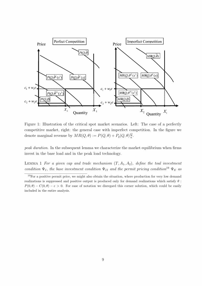
The critical spot market scenarios17 θB, θP , θP indicate wether firms produce either at
the capacity bounds x2, x1 (that is, at the vertical pieces of their marginal cost curves),
or on the flat (i.e. unconstrained) parts of their marginal cost curves. They depend on
the intensity of competition at the spot market and are illustrated in Figure 1 both for
the case of perfect and imperfect competition. For θ ∈ [θ, θB] firms produce the output at
marginal cost c2. For θ ∈ [θB, θP ] firms are constrained by their investment in the base load
technology and produce X2, still at marginal cost c2, and prices are driven by the demand
function. At those demand levels, using the peak load technology 1 is not yet profitable.
Observe that F (θP )−F (θB) measures the fraction of time where investment in the base load
technology is binding, which we will refer to as constrained base duration. For θ ∈ [θP , θP ]
firms produce output at marginal cost c1, we denote 1− F (θP ) as peak duration.18 Finally,
for all realizations above θP , firms are constrained by their total capacity choice X1, and
prices are driven exclusively by the demand function, we denote 1 − F (θP ) as constrained
17For the precise definition of those critical spot market scenarios, see appendix A.18The equivalent base duration would be given by 1− F (θ) = 1, it is not explicitly introduced, however.
8
Figure 1: Illustration of the critical spot market scenarios. Left: The case of a perfectly
competitive market, right: the general case with imperfect competition. In the figure we
denote marginal revenue by MR(Q, θ) := P (Q, θ) + Pq(Q, θ)Qn.
peak duration. In the subsequent lemma we characterize the market equilibrium when firms
invest in the base load and in the peak load technology.
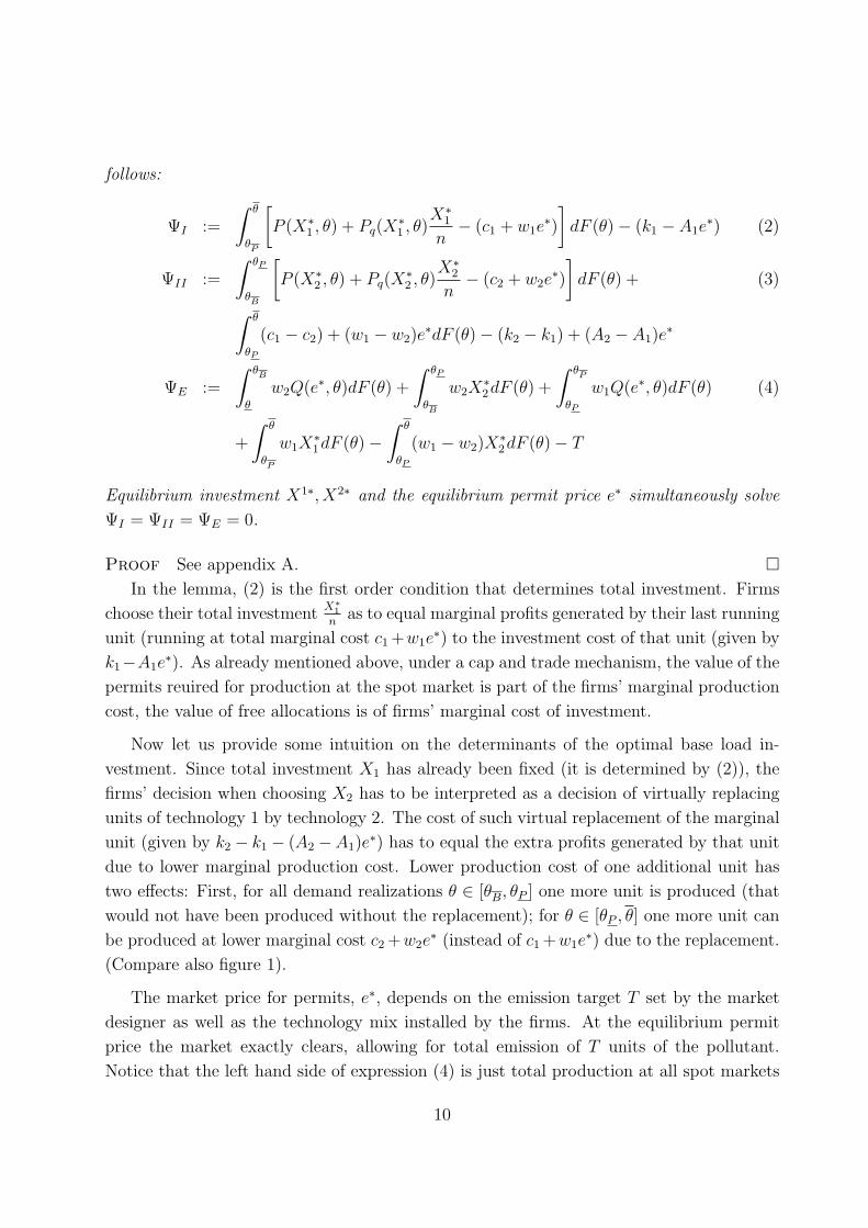
Lemma 1 For a given cap and trade mechanism (T,A1, A2), define the toal investment
condition ΨI , the base investment condition ΨII and the permit pricing condition19 ΨE as
19For a positive permit price, we might also obtain the situation, where production for very low demand
realizations is suppressed and positive output is produced only for demand realizations which satisfy θ :
P (0, θ) − C(0, θ) − e > 0. For ease of notation we disregard this corner solution, which could be easily
Equilibrium investment X1∗, X2∗ and the equilibrium permit price e∗ simultaneously solve
ΨI = ΨII = ΨE = 0.
Proof See appendix A. In the lemma, (2) is the first order condition that determines total investment. Firms
choose their total investmentX∗
1
nas to equal marginal profits generated by their last running
unit (running at total marginal cost c1+w1e∗) to the investment cost of that unit (given by
k1−A1e∗). As already mentioned above, under a cap and trade mechanism, the value of the
permits reuired for production at the spot market is part of the firms’ marginal production
cost, the value of free allocations is of firms’ marginal cost of investment.
Now let us provide some intuition on the determinants of the optimal base load in-
vestment. Since total investment X1 has already been fixed (it is determined by (2)), the
firms’ decision when choosing X2 has to be interpreted as a decision of virtually replacing
units of technology 1 by technology 2. The cost of such virtual replacement of the marginal
unit (given by k2 − k1 − (A2 −A1)e∗) has to equal the extra profits generated by that unit
due to lower marginal production cost. Lower production cost of one additional unit has
two effects: First, for all demand realizations θ ∈ [θB, θP ] one more unit is produced (that
would not have been produced without the replacement); for θ ∈ [θP , θ] one more unit can
be produced at lower marginal cost c2+w2e∗ (instead of c1+w1e
∗) due to the replacement.
(Compare also figure 1).
The market price for permits, e∗, depends on the emission target T set by the market
designer as well as the technology mix installed by the firms. At the equilibrium permit
price the market exactly clears, allowing for total emission of T units of the pollutant.
Notice that the left hand side of expression (4) is just total production at all spot markets
10
multiplied by the emission factors of the respective Technologies (w1, w2), total emissions
are obtained by integrating over emissions at all spot markets θ ∈ [θ, θ].
Finally observe that lemma 1 characterizes the market solution when firms decide to
invest in both technologies, that is, when indeed 0 < X∗2 < X∗
1 obtains. First, whenever
the base load technology (k2, c2) is very unattractive,20 then only the peak load technology
(k1, c1) is active. Second, if the base load technology (k2, c2) is always more attractive21
than the peak load technology (k1, c1), then only technology (k2, c2) is active in the market
equilibrium. Notice that in principle the case of investment in a single technology is cov-
ered by out framework, it obtains by eliminating the possibility to invest in technology 2,
expression (2)) then determines investment in the single technology. To keep the notational
burden limited, however, we do not explicitly include those corner solution in the exposition
of the paper, but opted to focus on all those cases when firms indeed choose to investment
in both technologies.
To conclude the discussion of lemma 1 let us already at this point mention the rele-
vance of endogenously modeling the emission permit market as compared to the case which
assumes an exogenously fixed price for pollution. Observe that, for a constant emission
price equilibrium investment under imperfect competition differs from that obtained under
perfect competition by the terms∫ θ
θPPq(X1, θ)
X1
nand
∫ θPθB
Pq(X2, θ)X2
ndF (θ) respectively,
which corresponds to the difference between scarcity prices and marginal scarcity profits.
Since those terms are negative (and profits concave given our assumptions) investment in-
centives under imperfect competition are lower than under perfect competition. That is,
in the absence of an explicit market for emission permits (when pollution is for example
taxed at some fixed level e0) subsidies for investment (for example by granting free tax
vouchers A1 > 0 and A2 > A1 respectively) which exactly compensate for those differences
would induce optimal investment incentives. Since the emission price is endogenous in our
framework, however, we will obtain a different result (compare theorem 2).
Before we now discuss existence of the market equilibrium we introduce the follow-
ing definitions which will simplify the subsequent analysis and allow for a more intuitive
discussion of our results:
Definition 1 (i) We denote the impact of increased total investment on total emissions
(for fixed e) by AE1 := ∂ΨE
∂X∗1= (1− F (θP ))w1, observe AE
1 > 0. This allows to state
the impact of changed emission price e∗ on the equilibrium condition ΨI as follows∂ΨI
∂e∗= A1 − AE
1 .
20That is expression (3) yields X∗2 ≤ 0.
21That is expressions (3) and (2) yield X∗2 ≥ X∗
1 .
11
(ii) We denote the impact of increased base load investment on total emissions (for fixed
e) by AE2 := ∂ΨE
∂X∗2= (1− F (θB))w2 − (1− F (θP ))w1. This allows to state the impact
of changed emission price e∗ on the equilibrium condition ΨII as follows ∂ΨII
∂e∗=
A2 − A1 − AE2 . We furthermore denote wE
2 :=1−F (θP )
1−F (θB)w1 (which implies AE
2 > 0
if and only if w2 > wE2 ) and wL
2 :=F (θP )−F (θP )
1−F (θB)w1 (which implies AE
1 +AE2 > 0 if and
only if w2 > wL2 ).
(iii) We denote the impact of changed X1 on the equilibrium condition ΨI by ΨI1 :=∂ΨI
∂X∗1,
the impact of changed X2 on the equilibrium condition ΨII by ΨII2 := ∂ΨII
∂X∗2
and the
impact of changed e on the equilibrium condition ΨE by ΨEe := ∂ΨE
∂e∗. Observe that
those three expressions are negative.
Observe22 that AE1 = (1− F (θP ))w1 determines the total amount of additionally neces-
sary permits resulting from an additionally invested unit of total capacity (formally given
by the partial derivative of total emission with respect to X1, i.e.∂ΨE
∂X1). An increase of
the permit price e now has two opposing effects on total investment incentives: on the one
hand investment incentives are reduced by the amount AE1 , on the other hand they increase
by A1 due to the increased value of free allocations.
A similar reasoning obtains for investment incentives in the base load technology. AE2
determines the total amount of additionally necessary permits resulting from the replace-
ment of one unit of the peak technology with one unit of the base technology (formally
given by the partial derivative of total emission with respect to X2, i.e.∂ΨE
∂X2). An increase
of the permit price e has two opposing effects on total investment incentives: on the one
hand they are reduced by the amount AE2 , on the other hand they increase by (A2 − A1)
due to the increased value of free allocations.
Notice that AE1 ≥ 0 whereas AE
2 can also become negative. That is, an increased level of
total investment X∗1 always implies additionally necessary emission permits. An increased
level of base investment X∗2 does only imply additionally necessary emission permits if
the base technology is “dirtier” than the peak technology. Interestingly the cut–off point
obtains for w2 = wE2 < w1, since an increased level of X∗
2 leads to increased emissions for
θ ∈ [θP , θ] if w2 > w2 but also leads to one unit of additional output for the demand levels
θ ∈ [θB, θP ].
As already argued, lemma 1 only characterizes the market equilibrium by establishing
necessary conditions. In the subsequent lemma ne now want to establish conditions second
order conditions for the existence of the market equilibrium.
22Notice that the statements of definition 1 and the subsequent discussion exclusively refer to partial
derivatives. In equilibrium total emissions do not change since they are capped at T .
12
Lemma 2 (Second Order Conditions) (i) Lemma 1 characterizes the market equi-librium if
(a)(A1 −AE
1
)AE
1 −ΨI1ΨEe < 0, (b)(A2 −A1 −AE
2
)AE
2 −ΨII2ΨEe < 0
(c)((A1 −AE
1
)AE
1 −ΨI1ΨEe
) ((A2 −A1 −AE
2
)AE
2 −ΨII2ΨEe
)>(A1 −AE
1
)AE
1
(A2 −A1 −AE
2
)AE
2
(ii) If the levels of free allocation satisfy(A1 − AE
1
)AE
1 ≤ 0 and(A2 − A1 − AE
2
)AE
2 ≤ 0,
then condition (i) is satisfied.
(iii) Define by Alim1 the highest A1 yielding
(A1 − AE
1
)AE
1 −ΨI1ΨEe ≤ 0, define by Alim2 the
highest A2 yielding(A2 − AE
1 − AE2
) (AE
1 + AE2
)− (ΨI1 +ΨII2)ΨEe ≤ 0. The second
order conditions (i) cannot be satisfied if either A1 ≥ Alim1 , or A2 ≥ Alim
1 .
Proof See appendix B. Part (i) of the lemma establishes the standard second order conditions which establishes
negative semi–definiteness of the Hessian matrix of firms’ optimization problem. It allows
the usual application of the implicit function theorem in order to conduct an analysis of
comparative statics for the equilibrium characterized in lemma 1. In part (ii) we establish
conditions when those second order conditions are satisfied and part (iii) provides an upper
bound on the levels of free allocation such that higher allocations always violate those
second order conditions.
Let us explicitly mention at this point that our analysis throughout this article focuses
on symmetric investment decisions, the second order conditions established in lemma 2(i)
guarantee that lemma 1 characterizes a unique symmetric solution. Since for the case of a
monopolistic or a perfectly competitive market asymmetric investment levels are irrelevant23
lemma 2(i) guarantees a existence and uniqueness of the market equilibrium in those cases.
For the case of oligopoly, when firms behave strategically, asymmetric investment levels
might be relevant, however. Indeed, as we show in a companion paper (Zoettl(2010))
for investment decisions in a discrete number of technologies symmetric equilibria can only
exist if technologies are sufficiently different, for sufficiently similar technologies a symmetric
equilibrium of the investment game always fails to exist and asymmetric equilibria might
arise.24
23For perfect competition observe that both marginal cost of investment and marginal cost of production
are constant, for monopoly observe that asymmetries cannot arise by definition.24As analyzed in Zoettl(2010) those problems can be overcome when firms are allowed to choose from
a continuum of technologies, when existence and uniqueness of the symmetric equilibrium can be reestab-
lished. Those findings to some extend seem to be parallel the discussion on supply function equilibria, where
Klemperer and Meyer (1989) show existence and uniqueness of the market equilibrium when firms can bid
smooth supply functions, whereas von der Fehr and Harbord (1993) show than a symmetric equilibrium in
discrete step functions fails to exist.
13
After having established the market equilibrium, we now determine the impact of chang-
ing the parameters of the cap and trade mechanism (A1, A2, T ) in an analysis of comparative
statics. If the second order conditions specified in lemma 2 (i) are satisfied we obtain the
following results:
Lemma 3 (Comparative Statics of the market Equilibrium) (i) Higher
free allocation for the base load technology A2 always yields higher investment
in the base load technology (i.e. dX2
dA2> 0). We furthermore obtain dX1
dA2< 0
if and only if(A1 − AE
1
)AE
2 < 0. Define Across1 as the highest A1 yielding(
A1 − AE1
)AE
2 ≤ ΨEeΨI1 −(A1 − AE
1
)AE
1 , we obtaindX∗
2
dA2<
dX∗1
dA2if and only if(
w2 > wE2
)and A1 ∈ (Across
1 , Alim1 ).
(ii) Higher free allocation for the peak load technology A1 always yields higher investment
in the peak load technology (i.e. dX1
dA1> dX2
dA1). Define by Atotal
2 the highest A2 which
yields(A2 − AE
1 − AE2
)AE
2 − ΨII2ΨEe ≤ 0 and by Across2 the highest A2 which yields(
A2 − AE1 − AE
2
)AE
1 − ΨI1ΨEe ≤ 0. There exists a unique wS2 with wE
2 < wS2 ≤ w1
such thatdX∗
1
dA1< 0 if and only if w2 > wS
2 and A2 ∈ (Atotal2 , Alim
2 ). Furthermore, we
obtaindX∗
2
dA1> 0 if and only if w2 < wS
2 and A2 ∈ (Across2 , Alim
2 ).
(iii) For a change of the total emission cap T we obtaindX∗
1
dT> 0 if and only if
(A1 < AE
1
),
we furthermore obtaindX∗
2
dT> 0 if and only if (A2 − A1 < AE
2 ).
Proof See appendix C. As we establish in the theorem, an increase of the free allocation A2 in the base load
technology always leads to increased base load investment (i.e.dX∗
2
dA2> 0, see point (i)),
an increase of the free allocation A1 in the peak load technology always leads to increased
investment in the peak load technology (i.e.dX∗
1
dA1>
dX∗2
dA1, see point (ii)). The impact of
such changes on the remaining investment decisions is more ambiguous. In the subsequentparagraphs we briefly sketch the central trade-offs, a complete proof is only provided inthe appendix, however. First consider a variation of the free allocation A2 and determineits impact on the system of equilibrium conditions established in lemma 1. The totaldifferential yields:25
dΨI
dA2= ΨI1
dX∗1
dA2+ΨIe
de∗
dA2= 0 (5)
dΨII
dA2= ΨII2
dX∗2
dA2+ΨIIe
de∗
dA2+
∂ΨII
∂A2= 0 (6)
dΨE
dA2= ΨE1
dX∗1
dA2+ΨE2
dX∗2
dA2+ΨEe
de∗
dA2= 0 (7)
25For a better traceability of our computations we denote the partial derivatives ∂ΨI
∂e∗ = ΨIe,∂ΨII
∂e∗ = ΨIIe,∂ΨE
∂X∗1= ΨE1 and ∂ΨE
∂X∗2= ΨE2, in a second step we make use of AE
1 and AE2 introduced in definition 1.
14
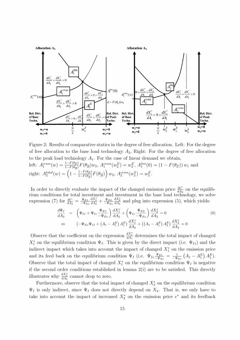
Figure 2: Results of comparative statics in the degree of free allocation. Left: For the degree
of free allocation to the base load technology A2, Right: For the degree of free allocation
to the peak load technology A1. For the case of linear demand we obtain,
left: Across1 (w) =
1−F (θP )
1−F (θB)F (θB)w2, A
cross1 (wE
2 ) = wE2 , A
lim1 (0) = (1− F (θP ))w1 and
right: Atotal2 (w) =
(1− 1−F (θP )
1−F (θB)F (θB)
)w2, A
cross2 (wS
2 ) = wE2 .
In order to directly evaluate the impact of the changed emission price de∗
dA2on the equilib-
rium conditions for total investment and investment in the base load technology, we solve
expression (7) for de∗
dA2= ΨE1
−ΨEe
dX∗1
dA2+ ΨE2
−ΨEe
dX∗2
dA2and plug into expression (5), which yields:
dΨI
dA2=
(ΨI1 +ΨIe
ΨE1
−ΨEe
)dX∗
1
dA2+
(ΨIe
ΨE2
−ΨEe
)dX∗
2
dA2= 0 (8)
⇔(−ΨEeΨI1 +
(A1 −AE
1
)AE
1
) dX∗1
dA2+((A1 −AE
1
)AE
2
) dX∗2
dA2= 0
Observe that the coefficient on the expressiondX∗
1
dA1determines the total impact of changed
X∗1 on the equilibrium condition ΨI . This is given by the direct impact (i.e. ΨI1) and the
indirect impact which takes into account the impact of changed X∗1 on the emission price
and its feed back on the equilibrium condition ΨI (i.e. ΨIeΨE1
−ΨEe= 1
−ΨEe
(A1 − AE
1
)AE
1 ).
Observe that the total impact of changed X∗1 on the equilibrium condition ΨI is negative
if the second order conditions established in lemma 2(i) are to be satisfied. This directly
illustrates whydX∗
2
dA2cannot drop to zero.
Furthermore, observe that the total impact of changed X∗2 on the equilibrium condition
ΨI is only indirect, since ΨI does not directly depend on X2. That is, we only have to
take into account the impact of increased X∗2 on the emission price e∗ and its feedback
15
on the equilibrium condition ΨI . According to definition 1 an increase of X2 leads to an
increased equilibrium emission price if AE2 > 0 (i.e. for w2 > wE
2 , we obtain a decreased
equilibrium emission price if AE2 < 0, i.e. for w2 < wE
2 ). The impact of an increased
emission price on the equilibrium condition ΨI depends on the the degree of free allocation
A1. Whenever A1 < AE1 (i.e. ∂ΨI
∂e∗< 0, compare definition 1) an increased emission price
leads to a decrease of firms’ total investment activity X∗1 . In this case the reduction of
scarcity rents (obtained when total capacity is binding) caused by the increased emission
price dominates the increased value associated to the permits granted for free. The reverse
holds true for a high level of free allocation, i.e. A1 > AE1 where an increased emission
price leads to increased total investment X∗1 . Whenever the impact of increased investment
X∗2 yields a decreased emission price, which obtains for cleaner base load technologies (for
AE2 < 0, i.e. w2 < wE
2 ), we obtain the opposite results. In sum,dX∗
1
dA2> 0 if and only if(
A1 − AE1
)AE
2 > 0, as stated in the theorem.
Finally expression (8) also provides the intuition under which conditions we obtaindX∗
1
dA2≥ dX∗
2
dA2(i.e. also investment in the peak load technology increases). To this end observe
thatdX∗
1
dA2=
dX∗2
dA2if and only if in expression (8) the total impact of changed X∗
1 is precisely
of the same size as the total impact of changed X∗2 , but of opposite sign. As shown in
the theorem this only obtains in case the increase of investment in the base technology
leads to an increase of the emission price (for AE2 > 0, i.e. w2 > wE
2 ) and if this increase
has a sufficiently positive impact on the equilibrium condition ΨI , i.e. for allocation A1
sufficiently big (for A1 > Across1 > AE
1 ). All those results are illustrated in the left graph of
figure 2.
Likewise we can analyze the impact of changing A1, as established in theorem 3(ii).
Analogous to expressions (19) (20) and (21) we can determine the total derivative and
solve for de∗
dA1. After plugging in, we obtain for dΨI
dA1+ dΨII
dA1(observe ∂ΨI
∂A1= −∂ΨII
∂A1= e):
dΨI
dA1+
dΨII
dA1=
(ΨI1 +ΨIe
ΨE1
−ΨEe+ΨIIe
ΨE1
−ΨEe
)dX∗
1
dA1+
(ΨII2 +ΨIIe
ΨE2
−ΨEe+ΨIe
ΨE2
−ΨEe
)dX∗
2
dA1= 0 (9)
⇔(−ΨEeΨI1 +
(A2 −AE
1 −AE2
)AE
1
) dX∗1
dA1+(−ΨEeΨII2 +
(A2 −AE
1 −AE2
)AE
2
) dX∗2
dA1= 0
Analogous to above the coefficients on the expressionsdX∗
2
dA1and
dX∗1
dA1determine the impact of
changed investment X∗1 or X∗
2 on both equilibrium conditions. The sum of both coefficients
is strictly negative if second order conditions are not to be violated (compare lemma 2(iii)).
This directly illustrates why dX2
dA1cannot reach the level of dX1
dA1(in other words, increased
free allocation A1 cannot leave investment in the peak load technology unchanged).
Furthermore, as we show, for small A2 both coefficients are negative (thusdX∗
1
dA1and
dX∗2
dA1
have opposite signs), sincedX∗
1
dA1>
dX∗2
dA1this implies
dX∗2
dA1< 0. Observe that the coefficient of
16
the expressiondX∗
1
dA1is increasing in A2, the coefficient of expression
dX∗1
dA1is increasing in A2 if
AE2 > 0 (i.e. w2 > wE
2 ). That is, for A2 high enough the coefficients become non–negative,
leading to altered monotonicity behavior. As we show in the theorem we can establish a
relative level of dirtiness wS2 (with wS
2 ≥ wE2 and wS
2 = wE2 in the case of linear demand),
which separates the cases when either of the coefficients becomes zero for higher levels of
A2 (Remember the sum of both coefficients has to be negative in order to satisfy the second
order conditions, see above). Whenever the coefficient ofdX∗
1
dA1equals to zero, expression (9)
directly impliesdX∗
2
dA1= 0 and vice versa, as stated in the theorem.
Finally, in theorem 3(iii) we provide the results of comparative statics with respect to
the parameter T . For an intuition of those results observe first of all that an increase of
the total emission cap T leads to a reduction of the equilibrium permit price. This in turn
induces increased total investment X∗1 if (similar to the intuition for part (i)) the increase
of scarcity rents (which obtains due to lower emission price) dominates the decreased value
of the emission permits granted for free, i.e. A1 < AE1 . The opposite result obtains for
A1 > AE1 . Similarly, the reduced emission price induces increased investment in the base
load technologyX∗2 if the total impact of reduced emission price on the base load investment
condition is negative, i.e. if and only if A2 < A1 + AE2 (i.e. ΨIIe < 0). If we denote total
emissions which obtain in the absence of any environmental policy by T . Lowering the cap
on total emissions T below T corresponds to the introduction of a cap and trade mechanism.
To provide the direct connection of our framework with current practice in competition
policy, let us conclude this section by briefly discussing the impact of introducing a cap and
trade mechanism as observed for example during the current phase of the EU ETS. In this
phase, the free allocations granted for free to a unit of each class of technologies were such
as to cover the total needs necessary on average to operate that unit.26 In our framework
that would correspond to levels of free allocation Afull1 ∈ [1 − (F (θP ))w1, 1 − (F (θP ))w1]
and Afull2 ∈ [1− (F (θB))w2, w2].
27 With an allocation scheme (Afull1 , Afull
2 ) which aims at
covering the average total needs of a unit of specific technology we obtain increased total
investment and increased base load investment when introducing the trading system (i.e.
26To give a specific example: In the German electricity market free allocation is determined by a tech-
nology specific emission factor which measures average emissions per unit of electricity produced (0.365
tCO2/MWh for gaseous fuels and 0.750 tCO2/MWh for solid and liquid fuels) multiplied by a preestab-
lished technology specific average usage. For open cycle gas turbines in Germany the average usage is
established at 0.11 (i.e. 1000 hours per year), for coal and combined cycle gas turbines it is given by 0.86
(i.e. 7500 hours per year) and for lignite plants it is given by 0.94 (i.e. 8250 hours per year), See appendices
3 and 4 of German Parliament (2007).27To be precise, in our framework average usage of the base technology is 1
X∗2
∫ θBθ
Q∗(θ)dF (θ) + (1 −F (θB)), the average usage of the peak technology is 1
X∗1−X∗
2
∫ θPθP
(Q∗(θ)−X∗2 ) dF (θ) + (1 − F (θP )). The
corresponding emission factors are given by w1 and w2 respectively.
17
the emission cap is lowered below T in our framework). To see this, first observe that
Afull1 > AE
1 which according to lemma 3 (iii) leads to an increase of X∗1 . Second observe
that Afull2 − Afull
1 > AE2 (since Afull
2 > (1 − F (θB))w2 and Afull1 < (1 − F (θP ))w1), which
according to lemma 3 (iii) leads to increased investment in the base load technology.
In order to apply our findings of lemma 3(i) consider again our example of an electricity
markets with lignite or coal fired plants as a representative base load technology and open
cycle gas turbines as a representative peak load technology. Since open cycle gas turbines
have lower emission factors, we obtain w2 > w1, which directly implies w2 > wE2 (compare
definition 1). Since furthermore Afull1 > AE
1 as established above, we can directly conclude
that an increase (decrease) of the free allocation A2 not only would yield increased base
load investment but also an increased (decreased) emission price and increased (decreased)
total investment.
After having analyzed the market equilibrium which obtains in the presence of an emis-
sion trading system and derived its properties of comparative statics we now proceed to the
main part of this article and analyze the optimal design of a cap and trade mechanism.
4 The Optimal Cap and Trade Mechanism
In this section we determine the optimal cap and trade mechanism. We first determine the
first best solution as a benchmark, which obtains for the case of a perfectly competitive
market when a regulator can freely choose all parameters (A1, A2, T ) of the cap and trade
mechanism (see theorem 1). We then analyze several market imperfections and solve for
the corresponding second best solutions. We first determine the optimal cap and trade
mechanism which should be chosen for an imperfectly competitive market (see section 4.1).
We then analyze the case when competition authorities cannot freely choose all parameters
(A1, A2, T ) of the cap and trade mechanism but only a subset of them (see section 4.2). In
order to answer all those questions we first determine total welfare generated in a market
with some cap and trade mechanism (A1, A2, T ):
W (A1, A2, T ) =
θB∫θ
[∫ Q∗
0
(P (Y, θ)− c2)Y dY
]dF (θ) +
θP∫θB
[∫ X∗2
0
(P (X∗2 , θ)− c2)Y dY
]dF (θ)
θP∫θP
[∫ Q∗
0
(P (Y, θ)− c1)Y dY
]dF (θ) +
θ∫θP
[∫ X∗1
0
(P (X∗1 , θ)− c1)Y dY
]dF (θ)
−θ∫
θP
(c1 − c2)X∗2dF (θ)− k2X
∗2 − k1(X
∗1 −X∗
2 )−D(T ). (10)
18
Observe, that welfare does not directly depend on the parameters (A1, A2, T ) chosen for
the cap and trade mechanism but only indirectly through the implied investment and
production decisions X∗1 , X
∗2 and Q∗. In order to maintain presentability of the results, we
relegated all computations to the appendix and directly characterize the optimal cap and
trade mechanism in the subsequent lemma.
Lemma 4 The optimal cap and trade mechanism solves the following conditions:
(i) WA1:=
dX∗1
dA1ΩI +
dX∗2
dA1ΩII = 0
(ii) WA2 :=dX∗
1
dA2ΩI +
dX∗2
dA2ΩII = 0
(iii) WT :=dX∗
1
dTΩI +
dX∗2
dTΩII −DT (T ) + e∗ +
∆
n= 0.
The expressions ΩI and ΩII determine the total impact of changed X∗1 and changed X∗
2
respectively on total Welfare. They are defined as follows:
ΩI :=
∫ θ
θP
−PqX∗1
ndF (θ)−A1e
∗ − ∆
nAE
1 ΩII :=
∫ θP
θB
−PqX∗2
ndF (θ)− (A2 −A1)e
∗ − ∆
nAE
2 .
The term ∆n
:=
∫ θB
θdQ∗de∗
(−Pq
Q∗n
)dF (θ)+
∫ θP
θP
dQ∗de∗
(−Pq
Q∗n
)dF (θ)∫ θ
Bθ ( dQ∗
de∗ w2)dF (θ)+∫ θ
PθP( dQ∗
de∗ w1)dF (θ)> 0 determines the impact of
changed emissions on welfare for those spot markets where investment is not binding.
Proof See appendix D. We now provide some intuition for the conditions which characterize an optimal cap and
trade mechanism. We first consider the optimal choice of the free allocation to the peak
load technology given by A1. Observe that the optimality conditions (i) and (ii) express
the impact of changed free allocation on total welfare exclusively through the channel of
changed investment in the base load technology X∗2 and changed total investment X∗
1 . The
total impact of changed investment on total welfare is denoted by ΩI and ΩII , this total
impact can be broken down into three components corresponding to the three summands
of ΩI and ΩII respectively.
First, observe that at all those spot markets where total investment is binding (i.e.
for θ ∈ [θB, θP ] and θ ∈ [θP , θ] respectively) imperfectly competitive investment behavior
induces too low investment incentives, an increase of investmentX∗2 orX∗
1 leads to increased
welfare given by the markup −PqXn. Second, free allocation A1 > 0 or (A2−A1) > 0 induces
too high investment incentives, thus an increase of investment would lead to a reduction
of welfare given by the monetary value of the free allocation (i.e. A1e∗ and (A2 − A1)e
∗).
Notice that in a world with exogenously fixed emission price e∗ the optimal level of free
allocation should be chosen such as to balance those two effects.28 Since the emission price
28That is, the monetary subsidy A1e∗ for example should then equate to the integral of the markups
over all relevant spot markets. The intuition for this result in some sense parallels the quite well known
19
is endogenous in our analysis, an additional term obtains. An increase of investment dX∗1
or dX∗2 leads to increased emissions of dX∗
1AE1 and dX∗
2AE2 at those spot markets where
investment is binding. Since total emissions are capped by T , however, this necessarily
has to imply an equivalent reduction of emissions at those spot markets where investment
is not binding (i.e. for θ ∈ [θ, θB] or θ ∈ [θP , θP ]). Since production decisions are also
imperfectly competitive, a reduction of output leads to reduced welfare generated at those
spot markets. This impact is quantified by the term ∆n
defined in the lemma. That is,
taking into account the endogenous nature of the emission price leads to a lower degree of
optimal free allocation A1 than suggested by an analysis with exogenously fixed emission
price.
The impact of a changed emission cap T on total welfare has a similar structure than
the impact of changed free allocations. Analogous to above, a changed emission cap leads
to changed investment incentives, the impact of changed investment incentives on welfare
is given by the terms ΩI and ΩII , which have already been discussed above. As we will
see later on in theorems 1 and 2, if the levels of free allocation are chosen optimally such
as to obtain ΩI = ΩII = 0 those terms will not be relevant for the optimal choice of the
emission cap. If the levels of free allocation are not chosen optimally, however, they have to
be considered when determining the optimal level of the emission cap T (compare theorems
3, 4, 5 and 6).
Apart from having an impact on investment incentives, a changed emission cap T leads
to changed welfare also through several other channels. First, most apparently an increased
emission cap leads to increased emissions which reduce welfare by the marginal social cost of
pollution DT . Second, observe that on the other hand an increased emission cap leads to a
welfare increase since it implies a reduced emission price which allows for increased output.
The welfare increase at each spot market is given by the changed output multiplied by
the difference between marginal cost as perceived by the firms and true marginal cost, i.e.
dQ(wie∗), for i = 1, 2. Put differently however, this corresponds to the changed pollution
at each spot market multiplied by the emission price e∗, the change in welfare at all spot
markets then is simply given by the total change of emissions multiplied by the emission
price i.e. dTe∗. As we will see in the subsequent theorem 1, for a perfectly competitive
market the optimal cap and trade mechanism only balances those two effects and equates
the marginal social cost of pollution to the emission price (i.e. e∗ = DT ).29 Third, observe
that an increased emission cap T leads to a reduced emission price. This allows to reduce the
insight obtained for a simple static model where a monopolist can be induced to produce first best output
if he obtains a subsidy corresponding to his markup.29This parallels the fundamental tradeoff obtained in a simple static model where a Pigou tax should
just equal to the marginal social damage of pollution.
20
welfare loss obtained due to imperfect competition at those spot markets where investment
is not binding and output too low. Notice that the impact of changed emissions on welfare
at those spot markets where investment is not binding has already been discussed above,
it is given by ∆n.
Based on the findings of lemma 4 as the first best benchmark we can now directly
establish the optimal cap and trade mechanism which obtains for a perfectly competitive
market
Theorem 1 (Optimal Market Design, First Best Benchmark) Under perfect
competition the optimal market design satisfies
(i) A∗1 = 0 (ii) A∗
2 = 0 (iii) T ∗ : e∗ = DT (T ).
Proof See appendix E. The theorem demonstrates that in a competitive market (i.e. n → ∞), full auctioning
is unambiguously optimal (i.e. no free allocations should be granted). A brief glance to
lemma 4 and the intuition provided reveals that investment incentives of firms under perfect
competition are optimal, positive free allocation would lead to reduced welfare. Moreover,
as condition (iii) shows, the emission target T should be set such that the equilibrium
permit price equals marginal social cost of environmental damage. That is, as already dis-
cussed above, the optimal cap and trade mechanism balances welfare losses due to foregone
production at all spot markets given by e∗ with the marginal social cost of pollution given
by DT .
in the subsequent two sections we now consider market imperfections which make an
attainment of the first best outcome impossible. First, we determine the design of an
optimal cap and trade mechanism for an imperfectly competitive market (see section 4.1).
Apart from imperfect competition, another source of market imperfection arises when the
competition authorities cannot freely choose all parameters (A1, A2, T ) of the cap and trade
mechanism, but only a subset. Such situations arise for example when the level of free
allocation for (some of) the different technologies or the total emission cap is exogenously
fixed due to political arrangements or lobbing of firms and the competition authority can
only determine the remaining parameters (see section 4.2).
4.1 Optimal Market Design under Imperfect Competition
After having determined the first best benchmark (theorem 1) we now determine the optimal
cap and trade mechanism for an imperfectly competitive market.
21
Theorem 2 (Optimal Market Design under Imperfect Competition) Under
imperfect competition the optimal market design satisfies
(i) A∗1 =
1
e∗
(∫ θ
θP
(−PqX
∗1
n
)dF (θ)− ∆
nAE
1
)
(ii) A∗2 =
1
e∗
(∫ θP
θB
(−PqX
∗2
n
)dF (θ) +
∫ θ
θP
(−PqX
∗1
n
)dF (θ)− ∆
n
(AE
1 +AE2
))
(iii) T ∗ : e∗ = DT (T )−∆
n.
Now assume that Pqθ = 0. We then obtain A∗1 > 0. For w2 ≤ wE
2 we obtain A∗2 > A∗
1, for
w2 > wE2 we can obtain A∗
2 = 0.
Proof See appendix E. The optimal levels of free allocations (A∗
1, A∗2) under imperfect competition are thus
typically different from zero, a striking difference to the result obtained under perfect com-
petition (see theorem 1). The fundamental reason why this is the case follows directly from
the insights provided by lemma 1 and the subsequent discussion of the results: Imperfectly
competitive firms not only exercise market power at the spot markets, but also choose their
capacity such that they optimally benefit from scarcity prices, implying reduced production
and investment incentives.
As already discussed in the text following lemma 1 (compare the last paragraph which
discusses lemma 1), for an exogenously fixed price for pollution (e.g. a pigouvian tax at
some fixed level e∗) optimal investment incentives are obtained by subsidizing investment
such as to precisely compensate for the difference between scarcity rents and marginal
scarcity profits. To stick as close as possible to our notation such subsidy could be made
by assigning the amounts A1 and A2 of free tax vouchers to each unit invested in either of
the technologies. The optimal level of tax vouchers is then given by expressions (i) and (ii)
of theorem 2 (notice that for exogenously fixed permit price we have ∆ = 0).
Remember that in our framework the expression ∆nallowed to quantify the impact of
changed emissions at those spot markets where investment is not binding. Positive free allo-
cation leads to increased investment incentives, which (through an increased emission price)
can lead to reduced output (and thus pollution) at those spot market where investment is
not binding. The terms including the expression ∆ntake this welfare loss into account. This
leads to a reduced level of the optimal degree of free allocation. As we show in the theorem,
under imperfect competition the degree of free allocation for the peak load technology is
always positive. For the optimal allocation for the base load technology ambiguous results
obtain. If the base load technology is less emission intensive than the peak load technology
(i.e. w2 ≤ w1) increased investment in the base load technology leads to reduced emissions
and thus allows for more output at spot markets where investment is not binding. As we
22
show this always implies A∗2 > A∗
1. On the other hand, if the base load technology is more
emission intensive than the peak load technology (w2 > w1, i.e. an increase of base load
investment leads to increased emission price), then it might be optimal to set A∗2 < A∗
1 or
even A∗2 < 0 as we show.
Finally consider the optimal choice of the total emission cap T for the case of imperfect
competition. A brief look at the optimality condition (iii) established in lemma 4 reveals,
that the impact of a changed emission cap on investment decisions can be neglected since the
levels of free allocation are determined optimally (such as to obtain ΩI = ΩII = 0). What
matters, however, is the fact that an increased emission cap leads to a reduced emission
price which in turn allows to reduce the welfare loss induced by imperfectly competitive
production decisions at those spot markets where investment is not binding (given by ∆n).
As a result the optimal cap on total emissions is chosen such as to yield an emission price
below the marginal social cost of pollution.
In sum, the main intuition why an optimal cap and trade mechanism (with endogenous
emission price) implies levels of free allocation which are different from zero is similar to the
intuition obtained for the case of an exogenously fixed price for pollution (e.g. a pigouvian
tax): Under imperfect competition firms’ investment and production incentives are too low,
leading to decreased welfare. Free allocations can provide adequate incentives which lead to
an increase of welfare. However, for the case of an endogenous emission price, as modeled
in the present paper, increased investment incentives also lead to an increased emission
price which in turn aggravates welfare losses at those spot market where investment is not
binding.
Let us finally discuss those results in the light of recently proposed measures thought
to increase firms’ investment incentives, as for example observed in liberalized electricity
markets. In the perception of many economists and policy makers investment incentives in
those markets are too low, one of the reasons potentially being market power as modeled
in the present paper. To resolve those problems of too low investment incentives, several
measures have been proposed, among them capacity mechanisms.30 For the present discus-
sion we clearly have to abstract form the specific problems encountered when designing real
capacity markets, and just consider some subsidy st paid to the firms per unit of invest-
ment made in technology t = 1, 2. Notice that in the present framework it is equivalent if
a monetary payment st or free allocations with value Ate∗ for t = 1, 2 are granted to a firm
per unit of investment in a technology t. What exclusively matters for firms’ investment
incentives is the total value st + Ate∗ granted to firms per unit of investment, this total
30In most restructured electricity markets in the United States so called ”capacity markets” are installed
in order to increase inefficiently low investment incentives, also in Europe policy makers consider their
introduction (see e.g. Cramton and Stoft (2008)).
23
value should be set at an optimal level.31
This in turn implies, however, that, once a cap and trade mechanism is put in place in
specific given market, the implications of this cap and trade have to be taken into account
when designing the capacity market. More specifically the design of a capacity market
which disregards the endogenous nature of emission prices, will lead to too high investment
incentives. However, we establish furthermore that also when taking into account the
endogenous nature of the emission price, the subsidy granted to the peak load technology
should be positive, if the base load technology is less emission intensive it should receive a
subsidy which exceeds that of the peak load technology. However, a relatively dirty base
load technology should not receive any free allocations.
4.2 Optimal Design of a Partially Constrained Cap and Trade
Mechanism
In theorems 1 and 2 we determined the optimal design of a cap and trade mechanism when
all its parameters (A1, A2, T ) can be freely chosen by the competition authority. We first
analyzed the case of a perfectly competitive market, which yields the first best benchmark
(theorem 1) and then the case of imperfect competition (theorem 2). Another source of
market imperfection, apart from imperfect competition, arises when the competition au-
thorities cannot freely choose all parameters (A1, A2, T ) of the cap and trade mechanism.
Such rigidities might be due to political constraints and arrangements or due to lobbing of
firms. As already discussed extensively in the introduction of this article free allocations
have been key to guarantee the political support necessary to introduce cap and trade sys-
tems, compare Convery(2009), Tietenberg(2006), Bovenberg (2008), or for example Grubb
and Neuhoff (2006)32. It is the purpose of the present section to analyze how a compe-
tition authority should optimally design a cap and trade mechanism if it can determine
only a subset of the parameters of the cap and trade mechanism, whereas the remaining
parameters are exogenously fixed due to the above discussed problems.
Theorem 3 determines the optimal degree of free allocations for the case of exogenously
31Consequently, optimality just requires that the sum of both parameters satisfies the above optimality
conditions. An immediate and interesting implication is that possible inefficiencies due to grandfathering
could be healed by capacity payments that compensate for the distorting effect without any efficiency losses
(as long as the subsidies resulting from free allocations are not higher than the sum of both parameters
should be).32“Due in part to the sheer scale of the EU ETS, governments are subject to intense lobbying relating to
the distributional impact of the scheme, and are constrained by this and by concerns about the impact of
the system on industrial competitiveness. Few academics understand the real difficulties that policy-makers
face when confronted with economically important industries claiming that government policy risks putting
them at a disadvantage relative to competitors.”
24
fixed level of the total emission cap T . In theorems 4, 5 and 6 we determine the optimal
degree of free allocation to the remaining technologies and the corresponding level of the
optimal total emission cap T . Observe that our results obtained in lemma 4 in principle
would allow for a detailed analysis of those questions both for the cases of perfect and
imperfect competition. In order to limit the notational burden in the present paper we
restrict ourselves to the case of perfect competition, however. In this case the optimality
conditions determined in lemma 4 read as follows
WA1:=
dX∗1
dA1(−A1) e
∗ +dX∗
2
dA1(A1 −A2) e
∗ = 0 (11)
WA2 :=dX∗
1
dA2(−A1) e
∗ +dX∗
2
dA2(A1 −A2) e
∗ = 0 (12)
WT :=dX∗
1
dT(−A1) e
∗ +dX∗
2
dT(A1 −A2) e
∗ −DT (T ) + e∗ = 0. (13)
We first analyze the case of an exogenously fixed level of the cap on total emissions T ,
an example might be a situation where politicians are willing to introduce a cap and trade
mechanism but are reluctant to induce too severe (even though optimal from an overall
welfare point of view) distortions on the economy. The above optimality conditions directly
reveal that in a perfectly competitive market no free allocations should be granted to firms,
independently of the level of the emission cap.33 This is summarized in theorem 3.
Theorem 3 (Optimal Design for fixed emission cap T ) For any exogenously fixed
total emission cap T it is optimal to choose the levels of free allocation A∗1 = A∗
2 = 0.
That is, the result obtained in the first best benchmark (theorem 1), where no free allocation
has been found to be optimal also obtains if the total emission cap is not set at an optimal
level. Observe that the reverse does not hold as we show in the subsequent theorem,
however.
Theorem 4 (Optimal Design for fixed allocations A1 and A2) Suppose the ini-tial allocations A1 and A2 are fixed exogenously. Define
Γ0(A1, A2) := (A1 −AE1 )A1ΨI1 + (A2 −A1 −AE
2 )(A2 −A1)ΨII2. (14)
The optimal emission cap T ∗ has to be set such as to satisfy e∗ = DT (T∗) for Γ0(A1, A2) =
0, e∗ > DT (T∗) for Γ0(A1, A2) > 0, and e∗ < DT (T
∗) for Γ0(A1, A2) < 0.
Proof See appendix F. That is, for levels of free allocation A1, A2 which are not set optimally the optimal cap
on emissions T typically does not implement an emission price e∗ equal to the social cost of
33The results of theorem 3 for the case of imperfect competition obtain analogously, the optimal levels
of free allocation are given by conditions (i) and (ii) established in theorem 2.
25
Figure 3: Choosing the optimal T ∗ for exogenously fixed initial allocations A1 and A2.
Left: for relatively dirty base technology, i.e. w2 > wE2 , Right: for relatively clean base
technology, i.e. w2 < wE2 .
pollution DT . To get an intuition for the result, note first that the cap T on total emissions
governs the price for emission certificates e∗, which in turn influences both investment
decisions and unconstrained production decisions at those spot markets where investment
is not binding. Optimal production decisions are induced by an emission price equal to the
social cost of pollution. This is only overall optimal in case of optimal investment incentives.
Now first observe that in case of positive free allocations (as considered in the theorem)
investment incentives are distorted, however. That is, for A1 > 0 investment incentives in
the peak load technology are too high, for A2 > A1 (A2 < A1) investment incentives in the
base load technology are too high (low). A distortion of the emission price can then be
suited to at least partially adjust investment incentives.
Second observe that the impact of a changed emission cap T on investment incentives
already has been derived in lemma 3 (iii) and discussed in the subsequent text. As estab-
lished there a higher emission cap T (implying a lower emission price e∗) leads to increased
investment in the peak load technology X∗1 if and only if A1 < AE
1 , it leads to increased
investment in the base load technology X∗2 if and only if A2 < A1 + AE
2 .
Intuitively theorem 4 formally joins those two effects, that is, whenever the levels of
26
free allocation A1, A2 are such as to induce over investment, the total cap on emissions
should be set such as to induce an emission price which leads to a reduction of investment
incentives and vice versa. All those findings are illustrated graphically in figure 3.
Consider the case A2 = A1 > 0, where all technologies get the same amount of free
allocations (the 45-degree line of figure 3). In the light of the above discussion this implies
first of all that investment incentives in the base load technology are undistorted (since
A2 = A1) and investment incentives in the peak load technology are too high. For A1 < AE1
investment incentives are reduced for a higher emission price, for A1 > AE1 they are reduced
for a lower emission price. Next consider the case A2 = A1 + AE2 . In this case a changed
emission price e∗ has no impact on investment in the base load technology, analogous
to above the optimal cap T is thus designed exclusively such as to reduce the too high
investment incentives in the peak load technology (i.e. for A1 < AE1 we have e∗ > DT and
vice versa).34
We conclude the discussion of theorem 4 by applying our findings to the current policy of
full allocation (Afull1 , Afull
2 ) as observed during the current phase of the EU ETS and already
introduced at the end of section 3. Remember that we derived the following properties for
the levels of full allocation: Afull1 > AE
1 and Afull2 > Afull
1 + AE2 . As already discussed,
if we consider either lignite or coal fired plants as the representative base load technology
and open cycle gas turbines as the representative peak load technology we also obtain
Afull2 > Afull
1 . For our framework we thus obtain that the optimal cap on total emissions
has to be set such that the equilibrium permit price is lower than the social cost of pollution,
i.e. e∗ < DT .
In the subsequent theorem 5 we consider the case that only allocation for the peak load
technology A1 is exogenously fixed, allocation for the base load technology A2 and the total
emission cap T can be determined optimally, however.
Theorem 5 (Optimal Design for fixed allocation A1) Suppose the allocation for
the peak technology A1 is exogenously fixed. The optimal allocation for the base technology
then solves A∗2 =
dX∗2 /dA2−dX∗
1 /dA2
dX∗2 /dA2
A1. More specifically we obtain (see left graph of figure 4)A∗
2 = 0 if (Across1 ≤ A1 < Alim
1 )
0 < A∗2 < A1 if
((0 < A1 < AE
1 ) & (w2 < wE2 ))OR
((AE
1 < A1 < Across1 ) & (w2 > wE
2 ))
A1 < A∗2 if
((AE
1 < A1 < Across1 ) & (w2 < wE
2 ))OR
((0 < A1 < AE
1 ) & (w2 > wE2 )).
The optimal cap T ∗ is such that e∗ > DT if A1 < AE1 and e∗ < DT if A1 > AE
1 .
34Observe that an analogous reasoning obtains for the case A1 = 0, when only investment incentives in
the base load technology are distorted and the case A1 = AE1 , when a changed emission price has no impact
on investment in the peak load technology and only distortions of base load investment are to be adjusted
by the total emission cap.
27
Proof See appendix G.
Figure 4: Left: Choosing the optimal A∗2 for exogenously fixed initial allocation A1. Right:
Choosing the optimal A∗1 for exogenously fixed initial allocation A2.
Observe that the optimality condition for A2 as stated in the theorem obtains directly
by rearranging expression (12). To derive the properties of the optimal degree of allocation
for the base load technology A∗2 as stated in the theorem we can now make use of the
properties of comparative statics derived in lemma 3(i). Most importantly, as established
there, we always obtaindX∗
2
dA2> 0. We thus obtain A∗
2 > A1 if and only ifdX∗
1
dA2< 0. Since we
only consider non–negative levels of free allocation we furthermore obtain A∗2 = 0 whenever
0 <dX∗
2
dA2<
dX∗1
dA2. All those results of comparative statics have been derived in lemma 3 and
have been discussed subsequently in section 3. Figures 2 and 4 do thus in principle look
identical, observe however, that figure 2 exclusively states results of comparative statics,
whereas figure 4 illustrates the properties of the optimal allocation A∗2 by making use of
the previously obtained findings.
The Intuition for the optimal level of free allocation T ∗ in principle goes along the
same lines as the one provided for the findings of theorem F. As compared to the first best
benchmark, for positive allocation A1 investment incentives in the peak load technology are
too high. Whenever A1 < AE1 we obtain ΨIe < 0 which implies that a higher emission price
e∗ allows to reduce investment incentives in the peak load technology. Observe furthermore
that investment incentives in the base load technology as induced by A∗2 are either too high
or too low (i.e. A∗2 > A1 for w2 > wE
2 and vice versa). As we show in the theorem it is
28
optimal to set the total cap such as to obtain an emission price e∗ > DT which induce
reduced investment incentives in the peak load technology whenever A1 < AC1 . Observe
Hahn, R.W. and R.N. Stavins (2010). The Effect of Allowance Allocations on Cap-
and-Trade System Performance. NBER Working Paper 15854.
Harstad, B. and G. Eskeland (2010). Trading for the Future: Signaling in Permit
Markes. Journal of Public Economics, 94, 749–760.
Hintermann, B. (2011). Market Power, Permit Allocation and Efficiency in Emission
Permit Markets. Environmental and Resource Economics, forthcoming.
IEA (2010). Reviewing Existing and Proposed Emission Trading Systems. Interna-
tional Energy Agency. Paris, November 2010.
Klemperer, P. and M. Meyer (1989). Supply Function Equilibria in Oligopoly under
Uncertainty. Econometrica, 57, 1243–1277.
33
Mackenzie, I.A., N. Hanley, and T. Kornienko (2008). The Optimal Initial Allocation
of Pollution Permits: a Relative Performance Approach. Environmental Resource
Economics , 39, 265–282.
Matthes, F. (2006). Analyse der Wirtschaftlichkeit von Kraftwerksinvestitionen im
Rahmen des EU-Emissionshandels. Institute for Applied Ecology Working Paper.
Moledina, A.A., J.S. Coggins, S. Polasky, and C. Costello (2003). Dynamic environ-
mental policy with strategic firms: prices versus quantities. Journal of Environmental
Economics and Management 45, 356-376.
Montero, J. P. (2002). Permits, Standards, and Technology Innovation. Journal of
Environmental Economics and Management, 44, 23–44.
Neuhoff, K., K. Keats Martinez, and M. Sato (2006). Allocation, Incentives, and
Distortions: The Impact of EU ETS Emissions Allowance Allocations to the Energy
Sector. Climate Policy 6, 73–91.
Pahle, M., L. Fan, and W.–P. Schill (2011). How Emission Certificate Allocations
Distort Fossil Investments, the German Example. DIW-Discussion Paper 1097
Requate, T. and Unold, W. (2001). On the incentives of policy instruments to adopt
advanced abatement technology if firms are asymmetric. Journal of Institutional and
Theoretical Economics 157, 536-554.
Requate, T. and W. Unold (2003). Environmental Policy Incentives to Adopt Ad-
vanced Abatement Technology: Will the True Ranking Please Stand Up?. European
Economic Review, 47, 125–146.
Requate, T. (2005). Dynamic Incentives by Environmental Policy Instruments-a Sur-
vey. Ecological Economics, 54, 175–195.
Rosendahl, K.E. (2008). Incentives and Prices in an Emission Trading Scheme with
Updating. Journal of Environmental Economics and Management, 56, 69-82.
Tietenberg, T. (2006). Emissions Trading: Principles and Practice, second edition.
RFF Press.
Zottl, G. (2010). A Framework of Peak Load Pricing with Strategic Firms. Operations
Research, 58, 1637–1649.
Zottl, G. (2011). On Optimal Scarcity Prices. International Journal of Industrial
Organization, forthcoming.
34
A Proof lemma 1
Note that given our assumptions on demand and cost, existence of spot market equilibriumat each demand scenario θ is ensured for the case of perfect and imperfect competition.We denote by q∗i (θ, x) spot market output of firm i in scenario θ, given investments x =(x11, . . . , x1n, x21, . . . , x2n). Remember, X1 and X2 denote industry investment in eithertechnology and Q∗(θ) industry output at each spot market θ, it is given as follows:
The critical spot market scenarios are defined as follows:
θB : P (X2, θB) + Pq(X2, θB)1
n− c2 − w2e
∗ = 0
θP : P (X2, θP ) + Pq(X2, θP )1
n− c1 − w1e
∗ = 0
θP : P (X1, θP ) + Pq(X1, θP )1
n− c1 − w1e
∗ = 0
That is, at spot market θB investment X2 in the base–load technology (c2, k2) starts to
be binding, at θP firms start to produce with the peak–load technology (c1, k1) and at θPthe total capacity bound X1 is met. The first order conditions stated in lemma (1) obtain
when equating expressions (16), (17), and (18) to zero. Notice that the case solution for
the case perfect competition obtains as the special case where n → ∞.
We first derive the first order conditions for optimal investment decisions. Note that,although in equilibrium at different demand realizations θ firm i might sometimes producean unconstrained equilibrium quantity and sometimes is constrained by its choice x1i or x2i,equilibrium profit of firm i is continuous in θ. Thus, by Leibniz’ rule, the first derivativesof the profit function are given as follows:
In the market solution the emission price e has to be such as to equate the followingexpression to zero: ∫ θB
θ
w2Q∗dF (θ) +
∫ θP
θB
w2X2dF (θ) +
∫ θP
θP
w1Q∗dF (θ)
+
∫ θ
θP
w1X1dF (θ)−∫ θ
θP
(w1 − w2)X2dF (θ)− T (18)
35
Which are the conditions ΨI , ΨII and ΨE as given in the lemma.
Let us directly at this point determine all partial derivatives of the equilibrium systemcharacterized in the lemma. The partial derivatives of ΨI (expression (16)), ΨII (expression(17)) and ΨE (expression (18)) read as follows:
∂ΨI
∂X∗1
= ΨI1 =
∫ θ
θP
Pq (X∗1 , θ)
n+ 1
n+ Pqq (X
∗1 , θ)
X∗1
ndF (θ) < 0
∂ΨII
∂X∗2
= ΨII2 =
∫ θP
θB
Pq (X∗2 , θ)
n+ 1
n+ Pqq (X
∗2 , θ)
X∗2
ndF (θ) < 0
∂ΨE
∂e= ΨEe =
∫ θB
θ
w22
Pq(Q∗, θ)n+1n + Pqq(Q∗, θ)Q
∗
n
dF (θ) +
∫ θP
θP
w21
Pq(Q∗, θ)n+1n + Pqq(Q∗, θ)Q
∗
n
dF (θ) < 0
∂ΨE
∂X∗1
= ΨE1 = (1− F (θP ))w1 = AE1 > 0
∂ΨI
∂e= ΨIe = A1 − (1− F (θP ))w1 = A1 −AE
1
∂ΨE
∂X∗2
= ΨE2 = (1− F (θB))w2 − (1− F (θP ))w1 = AE2
∂ΨII
∂e= ΨIIe = A2 −A1 − (1− F (θB))w2 + (1− F (θP ))w1 = A2 −A1 −AE
2
∂ΨI
∂A1= e
∂ΨII
∂A1= −e
∂ΨII
∂A2= e
∂ΨE
∂T= −1.
B Proof lemma 2
Part (i): To derive the second order conditions established in lemma 2, first observe thatdifferentiation of the permit pricing condition ΨE with respect to X1 and slight rearrangingyields de∗
dX1= ΨE1
−ΨEe. Plugging into the derivatives of ΨI and ΨII and replacing for AE
1 and
AE2 as introduced in definition 1 yields:
dΨI
dX1= ΨI1 +ΨIe
ΨE1
−ΨEe= ΨI1 + (A1 −AE
1 )AE
1
−ΨEe
dΨII
dX1= ΨIIe
ΨE1
−ΨEe= (A2 −A1 −AE
2 )AE
1
−ΨEe
Likewise we obtain
dΨI
dX2= ΨIe
ΨE2
−ΨEe= (A1 −AE
1 )AE
2
−ΨEe
dΨII
dX1= ΨII2 +ΨIIe
ΨE2
−ΨEe= ΨII2 + (A2 −A1 −AE
2 )AE
2
−ΨEe
The matrix H =
(dΨI/dX1 dΨI/dX2
dΨII/dX1 dΨII/dX2
)is negative definite if and only if conditions
(a), (b) and (c) established in lemma 2 (i) are satisfied. To save on notation we introduce
C := det(H), observe that C ≥ 0 if H is negative definite (compare (c) in lemma 2 (i)).
Part (ii): Since ΨI1 < 0, ΨII2 < 0 and ΨEe < 0 (see appendix A) the conditions
provided in lemma 2 (ii) are sufficient to guarantee negative definiteness of the matrix H.
36
Part (iii): To see why this is true, just observe that for A1 > Alim1 condition (a)
established in lemma 2(i) will be violated. The condition defining Alim2 is given by the sum
of conditions (a) and (b) of lemma 2(i), for A1 > Alim1 at least one of those two conditions
will be violated.
C Proof lemma 3
C.1 Preliminaries: Comparative Statics
The differentials fordX∗
1
dA1,dX∗
1
dA2,dX∗
1
dT anddX∗
2
dA1,dX∗
2
dA2,dX∗
2
dT are obtained by applying the implicityfunction theorem to the equilibrium conditions established in lemma 1. The total derivativeof this equations system with respect to the parameter A1 yields:
ΨI : ΨI1dX∗
1
dA1+ΨIe
de∗
dA1+
∂ΨI
∂A1≡ 0 (19)
ΨII : ΨII2dX∗
2
dA1+ΨIIe
de∗
dA1+
∂ΨII
∂A1≡ 0 (20)
ΨE : ΨE1dX∗
1
dA1+ΨE2
dX∗2
dA1+ΨEe
de∗
dA1+
∂ΨE
∂A1≡ 0 (21)
In order to derive an explicit formulation fordX∗
1
dA1, we solve expression (21) for de∗
dA1and
expression (20) fordX∗
2
dA1. Plugging into expression (19) yields:(ΨI1 +ΨIe
ΨE1
−ΨEe
)−(ΨIe
ΨE2
−ΨEe
) (ΨIIe
ΨE1
−ΨEe
)(ΨII2 +ΨIIe
ΨE2
−ΨEe
) dX∗
1
dA1+
∂ΨI
∂A1−
(ΨIe
ΨE2
−ΨEe
)∂ΨII
∂A1(ΨII2 +ΨIIe
ΨE2
−ΨEe
) = 0
By making use of the definition of the variable C (compare appendix B) we can rearrangethis expression and obtain:
dX∗1
dA1= (−1)
∂ΨI
∂A1
(ΨII2 +ΨIIe
ΨE2
−ΨEe
)− ∂ΨII
∂A1
(ΨIe
ΨE2
−ΨEe
)C
=((A2 −AE
1 −AE2 )A
E2 −ΨII2ΨEe
) −e
−ΨEeC(22)
Likewise, to obtain an explicit formulation fordX∗
2
dA1, we analogously solve expression (21)
for de∗
dA1and expression (19) for
dX∗2
dA1. Plugging into expression (20) and solving for
dX∗2
dA1
yields:
dX∗2
dA1= (−1)
∂ΨII
∂A1
(ΨI1 +ΨIe
ΨE1
−ΨEe
)− ∂ΨI
∂A1
(ΨIIe
ΨE1
−ΨEe
)C
=((A2 −AE
1 −AE2 )A
E1 −ΨI1ΨEe
) e
−ΨEeC(23)
Analogously we obtain:
dX∗1
dA2=((A1 −AE
1 )AE2
) e
−ΨEeC
dX∗2
dA2=((A1 −AE
1 )AE1 −ΨI1ΨEe
) −e
−ΨEeC(24)
dX∗1
dT=(A1 −AE
1
) ΨII2
−ΨEeC
dX∗2
dT=(A2 −A1 −AE
2
) ΨI1
−ΨEeC
37
C.2 Proof lemma 3(i)
First, we define
Γlim1 (A1) := ΨI1 +ΨIe
ΨE1
−ΨEe=
∫ θ
θP
Pq(X∗1 , θ)dF (θ) +
(A1 −AE1 )A
E1∫ θB
θ
w22
−Pq(Q∗,θ)dF (θ) +∫ θPθP
w21
−Pq(Q∗,θ)dF (θ). (25)
Observe, that the second order sufficient conditions for existence of the market equilibrium
specified in 2(i) require Γlim1 (A1) < 0. Since Γlim
1 (A1) is increasing in A1 we can define a
unique Alim1 which solves Γlim
1 (Alim1 ) = 0 and conclude that
dX∗2
dA2> 0 for all A1 < Alim
1 .
Second, we define
Γtotal1 (A1) := ΨIe
ΨE2
−ΨEe=
(A1 −AE
1
)AE
2∫ θBθ
w22
−Pq(Q∗,θ)dF (θ) +∫ θPθP
w21
−Pq(Q∗,θ)dF (θ)(26)
This allows us to rewritedX∗
1
dA2as established in expression (24) as follows:
dX∗1
dA2= Γtotal
1 (A1)e∗
C(27)
We finally show that AE1 < Alim
1 . To see this, observe that Γlim1 (AE
1 ) = ΨI1 < 0. Since
Γlim1 (A1) is increasing in A1, we necessarily obtain Alim
1 > AE1 .
Third, we define
Γcross1 (A1) := ΨI1 +ΨIe
ΨE1
−ΨEe+ΨIe
ΨE2
−ΨEe=∫ θ
θP
Pq(X∗1 , θ)dF (θ) +
(A1 −AE
1
) (AE
1 +AE2
)∫ θBθ
w22
−Pq(Q∗,θ)dF (θ) +∫ θPθP
w21
−Pq(Q∗,θ)dF (θ)
Observe thatdX∗
2
dA2<
dX∗1
dA2if and only if Γcross
1 (A1) > 0 (compare expression (24)). We define
the locus where Γcross1 (A1) = 0 by Across
1 . We now compare the critical allocation Across1
relative to the critical values Alim1 and AE
1 :
• For w2 > wE2 , we can establish the following ranking: AE
1 < Across1 < Alim
1 .
To show the first inequality observe that for all A1 ≤ AE1 we obtain Γtotal
1 (A1) ≤ 0.
As shown above we also obtain Γlim1 (A1) ≤ 0, which implies Γcross
1 (A1) = Γlim1 (A1) +
Γtotal1 (A1) ≤ 0. This directly implies, however, that Across
1 cannot be in the interval
[0, AE1 ].
To show the second inequality observe that for A1 > AE1 we have Γtotal
1 (A1) > 0.
Whenever Γcross1 (A1) = Γlim
1 (A1) + Γtotal1 (A1) = 0 we must thus have Γlim
1 (A1) < 0.
Since Γlim1 (A1) is strictly increasing in A1 this implies Alim
1 > Across1 .
• For w2 < wE2 we establish that Γcross
1 (A1) < 0 (i.e. A∗1 > 0) for all A1 ∈ (0, Alim
1 ].
38
First, observe that for A1 > AE1 we obtain Γtotal
1 (A1) < 0, which implies that
Γcross1 (A1) = Γlim
1 (A1) + Γtotal1 (A1) < 0 for A1 ∈ [AE
1 , Alim1 ].
Second observe that for A1 ≤ AE1 and ((1− F (θB))w2 − (F (θP )− F (θP ))w1) > 0 we
obtain Γcross1 (A1) < 0.
Third observe that for A1 ≤ AE1 and ((1− F (θB))w2 − (F (θP )− F (θP ))w1) < 0,
Γcross1 (A1) is maximized for A1 = 0. Expression (28) then reads as follows:
Γcross1 (0) =
∫ θ
θP
Pq(X∗1 , θ)dF (θ) +
− (1− F (θP ))w1
((1− F (θB))w2 − (F (θP )− F (θP ))w1
)∫ θBθ
w22
−Pq(Q∗,θ)dF (θ) +∫ θPθP
w21
−Pq(Q∗,θ)dF (θ)
Which can be guaranteed to be negative if Pqq ≤ 0 and Pqθ ≥ 0. Without those
additional assumptions it might happen that A∗1 = 0 in the region where A1 ≤ AE
1
and ((1− F (θB))w2 − (F (θP )− F (θP ))w1) < 0.
C.3 Proof lemma 3(ii)
First, we define
Γlim2 (A2) :=
(ΨII2 +ΨI1 + (ΨIIe +ΨIe)
ΨE2 +ΨE1
−ΨEe
). (28)
In order to precisely define Alim2 first observe that ΨE2+ΨE1 = AE
1 +AE2 (compare definition
1), we thus have to consider the following two cases:
• For the case w2 > wL2 (i.e. AE
1 + AE2 > 0) Γlim
2 is strictly increasing in A2, we can
define a unique Alim2 which solves Γlim
2 (Alim2 ) = 0
• For the case w2 ≤ wL2 (i.e. AE
1 + AE2 ≤ 0) Γlim
2 (A2) is non-increasing in A2, it is thusminimized for A2 = 0, which yields
Γlim2 = ΨII2 +ΨI1 +
(A2 − (AE
1 +AE2 )) AE
1 +AE2
−ΨEe< 0.
That is, Γlim2 (A1) < 0 for all A2 ≥ 0. For ease of notation we thus define Alim
2 = ∞in this case.
We now determinedX∗
2
dA1− dX∗
2
dA1as given by expressions (22) and (22). After plugging in
for ∂ΨI
∂A1= e∗ and ∂ΨII
∂A1= −e∗ (compare appendix A) we obtain for
dX∗1
dA1− dX∗
2
dA1:((
ΨII2 +ΨIIeΨE2
−ΨEe
)+
(ΨIe
ΨE2
−ΨEe
)+
(ΨI1 +ΨIe
ΨE1
−ΨEe
)+
(ΨIIe
ΨE1
−ΨEe
))−e∗
C=
−e∗
CΓlim2 (A2)
Since Γlim2 (A2) < 0 as established above, we conclude that
dX∗1
dA1>
dX∗2
dA1for all A2 ∈ [0, Alim
2 ].
Second, we define
Γtotal2 (A2) :=
((ΨII2 +ΨIIe
ΨE2
−ΨEe
)+
(ΨIe
ΨE2
−ΨEe
))=
(ΨII2 +
(A2 −AE
1 −AE2
) AE2
−ΨEe
)(29)
39
• For w2 > wE2 (i.e. AE
2 > 0, see definition 1) Γtotal2 (A2) is strictly increasing in A2. Since
Γtotal2 (0) < 0, we can thus define a unique Atotal
2 > 0 which satisfies Γtotal2 (Atotal
2 ) = 0.
• For the case w2 ≤ wE2 (i.e. AE
2 ≤ 0, see definition 1) Γtotal2 (A2) is non-increasing in
A2. Observe that in this case Γtotal2 is maximized for (A2 = 0, w2 = 0) which yields:
Γtotal2 (0) =
(ΨII2 +
(A2 −AE
1 −AE2
) AE2
−ΨEe
)< 0. (30)
That is, for A2 ≥ 0 we obtain Γtotal2 (A2) < 0. For ease of notation we thus define
Atotal2 := ∞ whenever w2 ≤ wE
2 .
Observe now that we can rewritedX∗
1
dA1(established in expression (23)) in terms of Γtotal
2 ,which yields:
dX∗1
dA1= Γtotal
2 (A2)−e∗
C(31)
Third, we define
Γcross2 (A2) :=
(ΨI1 +ΨIe
ΨE1
−ΨEe
)+
(ΨIIe
ΨE1
−ΨEe
)= ΨI1 +
(A2 −AE
1 −AE2
) AE1
−ΨEe(32)
We now rewritedX∗
2
dA1as established in expression (23) in terms of Γcross
2 , which yields:
dX∗2
dA1= Γcross
2 (A2)e∗
C(33)
Observe that Γcross2 is strictly increasing in A2 (see appendix A). Since Γcross
2 (0) < 0, wecan thus define a unique Across
2 > 0 which satisfies Γcross2 (Across
2 ) = 0:
Across2 = AE
1 +AE2 +
ΨI1ΨEe
AE1
(34)
Finally we compare the different critical values: Alim2 , Atotal
2 , and Across2 . We have to
consider the following three cases:
• For w2 ≤ wL2 : In this case we obtain Γlim
2 (A2) < 0 and Γtotal2 (A2) < 0 for all A2 ≥ 0.
Thus Across2 provides the only critical level of initial allocation (remember, we defined
Alim2 = ∞ and Atotal
2 = ∞), we thus obtain Across2 < Alim
2 .
• For wL2 < w2 ≤ wE
2 : In this case we obtain Γtotal2 (A2) < 0 for all A2 ≥ 0 (remember, we
defined Atotal2 = ∞). Observe, furthermore that Γlim
2 (A2) = Γtotal2 (A2) +Γcross
2 (A2) for
all A2. This directly implies, however, that Γcross2 (Alim
2 ) > 0 and thus Across2 < Alim
2 .
40
• For w2 ≥ wE2 we evaluate Γtotal
2 (Across2 ), which yields (compare expressions (29)
and(34)):
Γtotal2 (Across
2 ) = ΨII2 −ΨI1AE
2
AE1
= P 2q
(F (θP )− F (θB)
)− P 1
q
(1− F (θB))w2 − (1− F (θP ))w1
w1(35)
Observe that we denote by P 1q the average slope of demand for those demand levels
where total investment is binding and by P 2q the average slope of demand for those
demand levels where base load investment is binding, i.e.:
(i) P 1q :=
θ∫θP
Pq(X∗1 , θ)dF (θ)
1− F (θP )(ii) P 2
q :=
θP∫θB
Pq(X∗2 , θ)dF (θ)
F (θP )− F (θB)(36)
Rearranged this yields:
Γtotal2 (Across
2 ) =−P 1
q (1− F (θB))
w1
w2 −
(1− F (θP )) + (F (θP )− F (θB))P 2
q
P 1q
1− F (θB)
w1
(37)
Now define
wS2 :=
(1− F (θP )) + (F (θP )− F (θB))P 2
q
P 1q
1− F (θB)w1 (38)
Observe, that wE2 < wS
2 ≤ w1 since F (θP ) − F (θB) > 0 and 0 <P 2q
P 1q
≤ 1, notice
that for P 2q = P 1
q (e.g. for Pqq = Pqθ = 0) we obtain wS2 = w1. Furthermore, for
w2 > wS2 we obtain Γtotal
2 (Across2 ) > 0 and for w2 < wS
2 we obtain Γtotal2 (Across
2 ) < 0.
Since Γlim2 (A2) = Γtotal
2 (A2) + Γcross2 (A2) for all A2 we obtain:
0 < Atotal2 < Alim
2 < Across2 if w2 > wS
2
0 < Atotal2 = Alim
2 = Across2 if w2 = wS
2
0 < Across2 < Alim
2 < Atotal2 if wE
2 < w2 < wS2
(39)
C.4 Proof lemma 3(iii)
Observe that we have deriveddX∗
1
dTand
dX∗2
dTin expression (24). The statements of lemma
3(iii) follow directly since ΨI1 < 0, ΨII2 < 0 and ΨEe < 0 (see definition 1).
D Proof lemma 4
To derive the optimal design of the cap and trade mechanism (A1, A2, T ) we first differ-entiate Welfare as given by expression (10) with respect to each of those parameters. We
41
obtain for dWdA1
:
dW
dA1=
∫ θB
θ
dQ∗
dA1[P (Q∗, θ)− c2] dF (θ) +
∫ θP
θP
dQ∗
dA1[P (Q∗, θ)− c1] dF (θ) +
dX∗2
dA1
[∫ θP
θB
[P (X∗2 , θ)− c2] dF (θ) +
∫ θ
θP
(c1 − c2)dF (θ)− (k2 − k1)
]+
dX∗1
dA1
[∫ θ
θP
[P (X∗1 , θ)− c1] dF (θ)− k1
]We can now plug in the equilibrium conditions for firms’ investment choices given byexpressions (2) and (3) and we can plug in the optimality conditions for the unconstrainedspot markets, whenever investment is not binding. 38 This yields:
dW
dA1=
∫ θB
θ
dQ∗
dA1
[−Pq
Q∗
n+ w2e
]dF (θ) +
∫ θP
θP
dQ∗
dA1
[−Pq
Q∗
n+ w1e
]dF (θ)
dX∗2
dA1
[∫ θP
θB
[−Pq
X∗2
n+ w2e
]dF (θ) +
∫ θ
θP
(w2 − w1)edF (θ)− (A2 −A1)e
]+
dX∗1
dA1
[∫ θ
θP
[−Pq + w1e] dF (θ)−A1e
]This can be further simplified by making use of the derivative of the permit pricing givenby expression 4 with respect to A1 (i.e. ΨE
A1. This allows to eliminate all terms containing
the emission factors w1 and w2 from the above expression (shown explicitly in expression(41) just below). We thus obtain
dW
dA1=
∫ θB
θ
dQ∗
dA1
[−Pq
Q∗
n
]dF (θ) +
∫ θP
θP
dQ∗
dA1
[−Pq
Q∗
n
]dF (θ) (40)
dX∗2
dA1
[∫ θP
θB
[−Pq
X∗2
n
]dF (θ)− (A2 −A1)e
]+
dX∗1
dA1
[∫ θ
θP
[−Pq
X∗1
n
]dF (θ)−A1e
]In order to show why indeed expression (40) is obtained, we now differentiate the permitpricing condition ΨE (compare lemma 1) with respect to A1, this yields
−∫ θB
θ
w2dQ∗
dA1dF (θ)−
∫ θP
θP
w1dQ∗
dA1dF (θ) = (41)
dX∗2
dA1
[∫ θP
θB
w2dF (θ) +
∫ θ
θP
(w2 − w1)dF (θ)
]+
dX∗1
dA1
[∫ θ
θP
w1dF (θ)
].
Now observe that dQ∗
dA1= dQ∗
de∗de∗
dA∗1, since unconstrained spot market output does not directly
depend on the degree of free allocation A1. By multiplying expression (41) with ∆ (asdefined in the lemma) we obtain:(∫ θB
θ
dQ∗
de∗
[−Pq
Q∗
n
]dF (θ) +
∫ θP
θP
dQ∗
de∗
[−Pq
Q∗
n
]dF (θ)
)de∗
dA1=
−∆
n
(dX∗
2
dA1AE
2 +dX∗
1
dA1AE
1
)(42)
38That is for spot markets θ ∈ [θ, θB ]∪ [θP , θP ], in those cases the optimality conditions are simply given
by P (Q∗, θ) + PqQ∗
n − ci − wie∗ = 0, for i = 1, 2.
42
We can now plug expression (42) into expression (40), which yields
dW
dA1=
−∆
n
(dX∗
2
dA1AE
2 +dX∗
1
dA1AE
1
)+
dX∗2
dA1
[∫ θP
θB
(−Pq
X∗2
n
)dF (θ)− (A2 −A1)e
]+
dX∗1
dA1
[∫ θ
θP
(−Pq
X∗1
n
)dF (θ)−A1e
]
Rearranging finally yields
dW
dA1=
dX∗2
dA1
[∫ θP
θB
(−Pq
X∗2
n
)dF (θ)− (A2 −A1)e−
∆
nAE
2
]+
dX∗1
dA1
[∫ θ
θP
(−Pq
X∗1
n
)dF (θ)−A1e−
∆
nAE
1
]
Which corresponds exactly to the expression for dWdA1
stated in the lemma. The very same
steps yield dWdA2
=dX∗
1
dA2ΩI +
dX∗2
dA2ΩII as stated in the lemma.
We finally determine dWdT
. Analogous to expression (40) we obtain:
dW
dT=
dX∗2
dT
[∫ θP
θB
[−Pq
X∗2
n
]dF (θ)− (A2 −A1)e
]+
dX∗1
dT
[∫ θ
θP
[−Pq
X∗1
n
]dF (θ)−A1e
](43)
∫ θB
θ
dQ∗
dT
[−Pq
Q∗
n
]dF (θ) +
∫ θP
θP
dQ∗
dT
[−Pq
Q∗
n
]dF (θ) + e∗ −DT (T )
Which obtains since all terms containing the emission factors w1 and w2 integrate to 1.Why this is the case becomes clear when differentiating the permit pricing condition ΨE
with respect to T :
−∫ θB
θ
w2dQ∗
dTdF (θ)−
∫ θP
θP
w1dQ∗
dTdF (θ) =
dX∗2
dTAE
2 +dX∗
1
dTAE
1 − 1.
Now observe that dQ∗
dT= dQ∗
de∗de∗
dT, since unconstrained spot market output does not directly
depend on the total emission cap T . By multiplying expression (44) with ∆nwe obtain:(∫ θB
θ
dQ∗
de∗
[−Pq
Q∗
n
]dF (θ) +
∫ θP
θP
dQ∗
de∗
[−Pq
Q∗
n
]dF (θ)
)de∗
dT=
−∆
n
(dX∗
2
dTAE
2 +dX∗
1
dTAE
1 − 1
)(44)
We can now plug expression (44) into expression (43), which yields after rearranging:
dW
dT=
dX∗2
dT
[∫ θP
θB
(−Pq
X∗2
n
)dF (θ)− (A2 −A1)e−
∆
nAE
2
]+
dX∗1
dT
[∫ θ
θP
(−Pq
X∗1
n
)dF (θ)−A1e−
∆
nAE
1
]+
∆
n+ e∗ −DT (T )
Which corresponds exactly to the expression for dWdT
stated in the lemma.
43
E Proof theorems 1 and 2
The optimality conditions established in lemma 4 are satisfied if the following conditions
hold:
ΩI =
∫ θ
θP
−PqX∗1
ndF (θ)−A1e
∗ − ∆
nAE
1 = 0
ΩII =
∫ θP
θB
−PqX∗2
ndF (θ)− (A2 −A1)e
∗ − ∆
nAE
2 = 0
e∗ = DT (T )−∆
n.
The case of perfect competition as analyzed in theorem 1 obtains for n− > infty. Observe
that elimination of all terms involving the number of firms n in the denominator in the
above conditions yields the characterization of the first best solution stated in theorem 1.
In order to obtain the solution obtained for the case of imperfect competition as established
in theorem 2 we solve the first two conditions for the levels of free allocation A1 and A2.
F Proof theorem 4
The optimality condition for T has been derived in lemma 4 (iii). After plugging in theresults of comparative statics for dX1
dT and dX2
dT derived in expression (24) we obtain:
e∗ −DT =
((A2 −A1)eΨIIe
ΨI1
−ΨEe C+A1eΨIe
ΨII2
−ΨEe C
)(45)
We now make use of the notation introduced in definition 1, which allows us to rewrite
expression (45) as follows:
e∗ −DT =((A2 −A1 −AE
2 )(A2 −A1)ΨII2 + (A1 −AE1 )A1ΨI1
) e∗
−ΨEe C(46)
Notice that e∗
−ΨEe C> 0 as established in appendix A. The remainder of the right hand side
of expression (46) states Γ0(A1, A2) as defined in expression (14). The expression e∗−DT (T )
and Γ0 do thus exhibit the same sign, which proofs the theorem.
G Proof theorem 5
As a first step we determine the properties of the optimal allocation A∗2. Observe that
the optimality condition A∗2 =
dX∗2 /dA2−dX∗
1 /dA2
dX∗2 /dA2
A1 stated in the theorem directly obtains by
rearranging expression (12). In lemma 3 (i) we have establisheddX∗
2
dA2> 0 for all A1 < Alim
1 .
We thus obtain A∗2 > A1 if and only if
dX∗1
dA2< 0. Furthermore, we obtain A∗
2 = 0 ifdX∗
2
dA2<
dX∗1
dA2since we only consider non–negative levels of free allocation. By making use
44
of the properties of comparative statics established in lemma 3 (i) we directly obtain the
properties of A∗2 as stated in the theorem.
As a second step we determine the optimal emission cap T ∗. The optimality condition
for T ∗ has been derived in expression (13) and yields after substituting for A∗2:
e∗ −DT =dX∗
1
dTA1e−
dX2
dTA1e
[dX1/dA2
dX2/dA2
].
After substituting for dX1
dT , dX2
dT , dX1
dA2, and dX2
dA2(expression (24)) this reads as follows:
e∗ −DT =
(ΨII2ΨIe)− (ΨI1ΨIIe)
(−ΨIe
ΨE2
ΨEe
)−(ΨI1 −ΨIe
ΨE1
ΨEe
) A1e
−ΨEe C
Rearranging and plugging in for ΨIe (compare appendix A) we obtain:
e∗ −DT =(AE
1 −A1
) (ΨI1
(ΨIIe
ΨE2
−ΨEe
)+ΨII2
(ΨI1 +ΨIe
ΨE1
−ΨEe
))A1e(
ΨI1 +ΨIeΨE1
−ΨEe
)ΨEe C
(47)
Observe that for A1 < Alim1 the sign of the right hand side of expression (47) is entirely
determined by the expression (AE1 −A1), the remainder of expression (47) is strictly positive
since(ΨI1 +ΨIe
ΨE1
−ΨEe
)< 0 and
(ΨIIe
ΨE2
−ΨEe
)< 0 (as shown further below in step three).
Finally notice that expression (47) has been derived without non–negativity constrainton A∗
2. As shown above, however, for w2 > wE2 and A1 ∈ [AE
1 , Alim1 ] we obtain A∗
2 = 0(instead of a negative value as resulting in the computations leading to expression (47)).In this case the optimality condition given by expression (13) simplifies as follows:
e∗ −DT =
(dX∗
1
dT− dX2
dT
)A1e = (ΨII2ΨIe −ΨI1ΨIIe)
A1e
−ΨEe C< 0 (48)
The inequality obtains since ΨIe > 0 and ΨIIe < 0 for w2 > wE2 and A1 ∈ [AE
1 , Alim1 ]
(compare appendix A). We thus summarize the results obtained in expressions (47) and
(54) as follows: e∗ > DT if A1 < AE
1
e∗ = DT if A1 = AE1
e∗ < DT if A1 > AE1
(49)
As a third step We finally show that the second order conditions established in lemma 2
(i) are indeed satisfied for all A1 ∈ [0, Alim1 ], A∗
2. Since(ΨI1 +ΨIe
ΨE1
−ΨEe
)< 0 for A1 < Alim
1
we just need to show that(ΨIIe
ΨE2
−ΨEe
)< 0 for A1 < Alim
1 . Notice first that we can rewrite
ΨIIe (compare appendixA) and thus obtain:
ΨIIeΨE2
−ΨEe= (A∗
2 −A1 −ΨE2)ΨE2
−ΨEe(50)
45
Furthermore, we obtain for (A∗2 − A1) (compare expressions (12) and (24)):
(A∗2 −A1) = −
dX1
dA2
dX2
dA2
A1 =
(ΨIe
ΨE2
−ΨEe
)A1(
ΨI1 +ΨIeΨE1
−ΨEe
)Plugging in allows us to rewrite expression (50) as follows:
ΨIIeΨE2
−ΨEe=
(ΨE2)2(
ΨI1 +ΨIeΨE1
−ΨEe
)(−ΨEe)
(ΨIe
A1
−ΨEe−(ΨI1 +ΨIe
ΨE1
−ΨEe
))
Substituting for ΨIe = A1 − AE1 and ΨE1 = AE
1 (see appendix A) then yields:
ΨIIeΨE2
−ΨEe=
(ΨE2)2(
ΨI1 +ΨIeΨE1
−ΨEe
)(ΨEe)
(ΨI1 −
(A1 −AE1 )
2
−ΨEe
)< 0
We can thus conclude that the second order conditions established in in lemma 2 (i) are
satisfied if and only if A1 < Alim1 (Notice that the “only if” part follows directly from lemma
2 (iii)).
H Proof theorem 6
As a first step we determine the properties of the optimal allocation A∗1. Observe that
the optimality condition A∗1 =
dX∗2 /dA1
dX∗2 /dA1−dX∗
1 /dA1A2 stated in the theorem directly obtains
by rearranging expression (11). In lemma 3 (ii) we have establisheddX∗
1
dA1>
dX∗2
dA1for all
A2 < Alim2 . We thus obtain A∗
1 > 0 if and only ifdX∗
2 /dA1
<0. Furthermore, we obtain
A∗1 > A2 if and only if
dX∗2
dA1<
dX∗1
dA1< 0. By making use of the properties of comparative
statics established in lemma 3 (ii) we directly obtain the properties of A∗1 as stated in the
theorem.
As a second step we determine the optimal emission cap T ∗. The optimality conditionfor T ∗ has been derived in expression (13) and yields after substituting for A∗
1 (comparethe first step above):
e∗ −DT =dX2
dT(A2 −A∗
1) e∗ +
dX∗1
dTA∗
1e∗ =
dX2
dT
dX1
dA1A2e
∗
dX1
dA1− dX2
dA1
+dX∗
1
dT−dX2
dA1A2e
∗
dX1
dA1− dX2
dA1
We can now plug in for dX1
dA1and dX2
dA1as derived in expressions (22) and (23) and for dX1
dTand dX2
dT as derived in expressions (24), which yields:
e∗ −DT =(−1)A2 (e
∗)2(dX1
dA1− dX2
dA1
)(−ΨEe)C2
((ΨIeΨII2)
[(ΨI1 +ΨIe
ΨE1
−ΨEe
)+
(ΨIIe
ΨE1
−ΨEe
)]+
(ΨIIeΨI1)
[(ΨII2 +ΨIIe
ΨE2
−ΨEe
)+
(ΨIe
ΨE2
−ΨEe
)])= (ΨIe +ΨIIe)
(−1)A2 (e∗)2(
dX1
dA1− dX2
dA1
)(−ΨEe)C
(51)
46
Now define:
Γem2 (A2) := ΨIe +ΨIIe = A2 − (AE
1 +AE2 ). (52)
Observe that Γem2 (Aem
2 ) = 0. Furthermore notice that Aem2 < 0 for w2 < wL
2 , that is,Γem2 (A2) > 0 for all A2 ≥ 0 whenever w2 < wL
2 . In order to compare Aem2 to the previously
established critical levels of initial allocation we make the following two observations:
Γtotal2 (Aem
2 ) = ΨII2 < 0 and Γcross2 (Aem
2 ) = ΨI1 < 0
This allows to directly conclude that Aem2 < Atotal
2 and Aem2 < Across
2 .
By making use of the newly introduced Γem2 we can rewrite expression (51) as follows:
e∗ −DT = −Γem2 (A2)
A2e∗(
dX1
dA1− dX2
dA1
)(−ΨEe)C
(53)
Finally notice that expression (53) has been derived without non–negativity constrainton A∗
1. As shown in step one of the present proof, however, for w2 < wS2 and A2 ∈
[Across2 , Alim
2 ] we obtain A∗1 = 0 (instead of a negative value as resulting in the computations
leading to expression (53)). In this case the optimality condition given by expression (13)simplifies as follows:
e∗ −DT =dX∗
2
dTA2e
∗ =ΨI1ΨIIe
−ΨEe CA2e
∗ =dX∗
2
dTA2e
∗ =(A2 −A1 −AE
2
) ΨI1 A2e∗
−ΨEe C< 0 (54)
Observe that the above inequality is satisfied, since A2 ≥ A1+AE2 whenever Across
2 ≤ A2 ≤Alim
2 (compare expression (34), remember that A1 = A∗1 = 0 in the case considered).
We can thus establish the following results for the optimal cap on total emissions:e∗ > DT if A2 < Aem
2
e∗ = DT if A2 = Aem2
e∗ < DT if A2 > Aem2
(55)
As a third step We finally show that the second order conditions established in lemma2(i) are indeed satisfied for all A2 ∈ [0, Alim
2 ], A∗1. Remember we obtained for A∗
1:
A∗1 =
Γcross2
Γlim2
A2 =Γcross2
Γcross2 + Γtotal
2
A2
In order to verify the second order conditions established in lemma 2(i) (a), (b), and (c)
we now separately analyze the following cases:
• First, observe that
ΨIIeΨE2
−ΨEe= (A2 −A1 −ΨE2)
ΨE2
−ΨEe=
(Γtotal2
Γlim2
A2 −ΨE2
)ΨE2
−ΨEe(56)
47
– For w2 < wE2 (i.e. ΨE2 < 0) expression (56) is negative, since Γtotal
2 < 0 and
Γlim2 < 0 if A2 < Alim
2 and w2 < wE2 (compare appendix C).
– For w2 > wE2 (i.e. ΨE2 > 0) and Atotal
2 ≤ A2 ≤ Alim2 expression (56) is negative,
since Γtotal2 ≥ 0 and Γlim
2 < 0.
Whenever expression(56) is negative this directly implies that condition (b) is satis-
fied. Since furthermore A2 < Alim2 also conditions (a) and (c) are satisfied.
• Second, for Across2 ≤ A2 ≤ Alim
2 we obtain A∗1 = 0 (compare step one of the present
proof). We thus directly obtain:
ΨIeΨE1
−ΨEe= −AE
1
ΨE1
−ΨEe< 0 (57)
This directly implies that condition (a) is satisfied. Since furthermore A2 < Alim2 also
conditions (b) and (c) are satisfied.
• Third, for w2 > wE2 (i.e. ΨE2 > 0) and 0 ≤ A2 ≤ min(Atotal