32
EMM Flow Diagram for structural model estimated parameters data simulated model auxiliary EMM model structural SNP observed data

EMM Flow Diagram
for structural modelestimated parameters
datasimulated
modelauxiliary
EMM
modelstructural
SNPobserved data

Simulate MA(1) Data Using gensim Function
MA1.gensim <- function(rho, n.sim=100, n.var=1, n.burn=25, aux=NULL) {
# simulate from MA(1) model # y(t) = e(t) - theta*e(t-1), e(t) ~ iid N(0,sigma^2) # rho = (theta,sigma2)' # aux is a list with components # innov = standard normals used for simulation # start.innov = standard normals used for start up values
ans = arima.sim(model = list(ma=rho[1]), innov = aux$innov*sqrt(rho[2]), start.innov = aux$innov.start*sqrt(rho[2]))
ans}

MA(1) Datatheta=-0.75, sigma=1
0 50 100 150 200 250
-20
2

MA(1) Data
Lag
AC
F
0 5 10 15 20
0.0
0.2
0.4
0.6
0.8
1.0
Series : MA1.sim
Lag
Par
tial A
CF
0 5 10 15 20
-0.2
0.0
0.2
0.4
Series : MA1.sim

MLE of MA(1)> MA1.data = MA1.sim - mean(MA1.sim) > mle.fit = arima.mle(MA1.data,model=list(ma=-0.5)) > mle.fit
Coefficients:MA : -0.76773
> mle.fit$sigma2[1] 0.8854201
> sqrt(mle.fit$var.coef)ma(1)
ma(1) 0.04052596
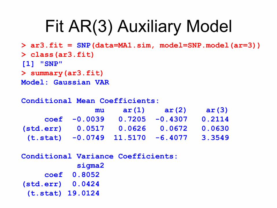
Fit AR(3) Auxiliary Model> ar3.fit = SNP(data=MA1.sim, model=SNP.model(ar=3))> class(ar3.fit)[1] "SNP"> summary(ar3.fit)Model: Gaussian VAR
Conditional Mean Coefficients:mu ar(1) ar(2) ar(3)
coef -0.0039 0.7205 -0.4307 0.2114(std.err) 0.0517 0.0626 0.0672 0.0630(t.stat) -0.0749 11.5170 -6.4077 3.3549
Conditional Variance Coefficients:sigma2
coef 0.8052(std.err) 0.0424(t.stat) 19.0124

Auxiliary Model Diagnostics-2
-10
12
0 50 100 150 200 250
MA1.sim
Std. Residuals versus Time
-3
-2
-1
0
1
2
3
-3 -2 -1 0 1 2 3
MA1.sim
Quantile of Standard Normal
Std
. Res
idua
ls
Normal Q-Q Plot
0.0
0.2
0.4
0.6
0.8
1.0
5 10 15 20
MA1.sim
Lag
AC
F
Std. Residual ACF
-0.15
-0.10
-0.05
0.0
0.05
0.10
5 10 15 20
MA1.sim
Lag
PA
CF
Std. Residual PACF

Simulation from Auxiliary Modelar3.sim = simulate(ar3.fit)
actual MA(1) data
0 50 100 150 200 250
-20
2
simulated data from fitted AR(3) model
0 50 100 150 200 250
-4-2
02

Diagnostics from Simulated Auxiliary Model
Lag
AC
F
0 5 10 15 20
-0.2
0.2
0.4
0.6
0.8
1.0
Series : ar3.sim
Lag
Par
tial A
CF
0 5 10 15 20
-0.2
0.0
0.2
0.4
Series : ar3.sim

EMM Fit of MA(1) Model# create inputs to MA1.gensim> set.seed(345) > z = rnorm(10000) > z.start = rnorm(100) > MA1.aux = list(innov = z, innov.start = z.start)
# fit MA(1) model using EMM> EMM.fit = EMM(ar3.fit,coef=c(-0.5,1), + control = EMM.control(n.burn=100,n.sim=10000), + gensim.fn="MA1.gensim2",gensim.language="SPLUS",+ gensim.aux=MA1.aux)
> class(EMM.fit)[1] "EMM"
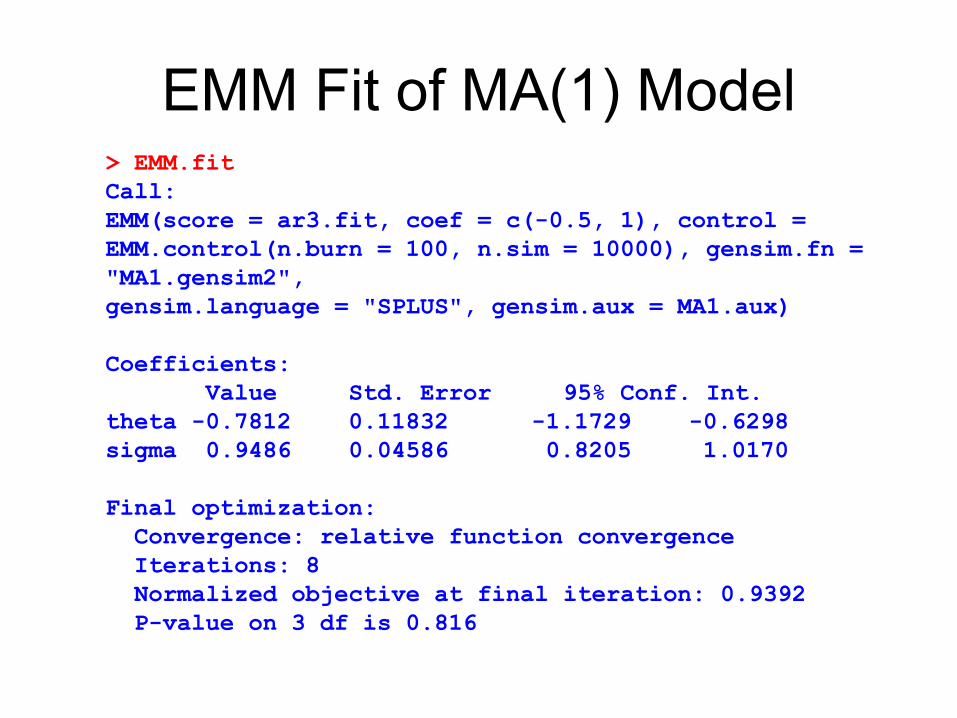
EMM Fit of MA(1) Model> EMM.fitCall:EMM(score = ar3.fit, coef = c(-0.5, 1), control = EMM.control(n.burn = 100, n.sim = 10000), gensim.fn = "MA1.gensim2", gensim.language = "SPLUS", gensim.aux = MA1.aux)
Coefficients:Value Std. Error 95% Conf. Int.
theta -0.7812 0.11832 -1.1729 -0.6298sigma 0.9486 0.04586 0.8205 1.0170
Final optimization:Convergence: relative function convergence Iterations: 8 Normalized objective at final iteration: 0.9392P-value on 3 df is 0.816

EMM DiagnosticsEMM Diagnostics
Score Std. Error t-ratio mu 1.15746942 1.241852 0.932051340
phi.1 0.03844991 1.267703 0.030330384phi.2 0.28548072 1.359517 0.209986938phi.3 0.17188357 1.197335 0.143555120sigma2 0.01452084 1.545968 0.009392714

Fit SNP 200100 Model> fit.200100 = SNP(tb3mo,model=SNP.model(ar=2),n.drop=6)> summary(fit.200100)
Model: Gaussian VAR
Conditional Mean Coefficients:mu ar(1) ar(2)
coef 0.0006 1.0911 -0.0969(std.err) 0.0036 0.0107 0.0109(t.stat) 0.1661 101.9655 -8.8810
Conditional Variance Coefficients:sigma
coef 0.0974(std.err) 0.0006(t.stat) 153.7107

Fit SNP 204100 Model> fit.204100 = expand(fit.200100,arch=4)> summary(fit.204100)
Model: Gaussian ARCH
Conditional Mean Coefficients:mu ar(1) ar(2)
coef 0.0009 1.0189 -0.0215(std.err) 0.0008 0.0188 0.0190(t.stat) 1.2491 54.3261 -1.1321
Conditional Variance Coefficients:s0 arch(1) arch(2) arch(3) arch(4)
coef 0.0211 0.4324 0.1358 0.3126 0.2879(std.err) 0.0007 0.0257 0.0191 0.0224 0.0231(t.stat) 28.5737 16.8110 7.1039 13.9848 12.4683

Diagnostics for SNP 204100-8
-6-4
-20
24
1965 1970 1975 1980 1985 1990 1995
tb3mo
Std. Residuals versus Time
-8
-6
-4
-2
0
2
4
-2 0 2
tb3mo
Quantile of Standard Normal
Std
. Res
idua
ls
Normal Q-Q Plot
0.0
0.2
0.4
0.6
0.8
1.0
0 5 10 15 20 25 30
tb3mo
Lag
AC
F
Std. Residual ACF
0.0
0.2
0.4
0.6
0.8
1.0
0 5 10 15 20 25 30
tb3mo
Lag
AC
F
Std. Residual^2 ACF

Simulation from SNP 204100T-bill data
1965 1970 1975 1980 1985 1990 1995
46
810
1214
16
simulated data from fitted SNP 204100 model
1965 1970 1975 1980 1985 1990 1995
-250
-150
-50
050

Fit SNP 211100 Model> fit.211100 = expand(fit.200100,arch=1,garch=1)> summary(fit.211100)
Model: Gaussian GARCH
Conditional Mean Coefficients:mu ar(1) ar(2)
coef -0.0014 1.0280 -0.0307(std.err) 0.0009 0.0230 0.0230(t.stat) -1.5642 44.7881 -1.3380
Conditional Variance Coefficients:s0 arch(1) garch(1)
coef 0.0023 0.2037 0.8383(std.err) 0.0001 0.0085 0.0050(t.stat) 27.0769 23.9992 167.7730

Fit SNP 211140 Model> fit.211140 = expand(fit.211100,zPoly=4)> summary(fit.211140)
Model: Semiparametric GARCH
Hermite Polynomial Coefficients:z^0 z^1 z^2 z^3 z^4
coef 1.0000 0.0754 -0.2025 -0.0065 0.0249(std.err) 0.0242 0.0163 0.0051 0.0025(t.stat) 3.1098 -12.4038 -1.2911 10.1074
Conditional Mean Coefficients:mu ar(1) ar(2)
coef -0.0065 1.0425 -0.0482(std.err) 0.0016 0.0251 0.0252(t.stat) -4.0240 41.5080 -1.9124
Conditional Variance Coefficients:s0 arch(1) garch(1)
coef 0.0021 0.2362 0.8367(std.err) 0.0001 0.0138 0.0069(t.stat) 15.2416 17.1264 121.0534

Fit SNP 211141 Model> fit.211141 = expand(fit.211140,xPoly=1)> fit.211141
Model: Nonlinear Nonparametric
Hermite Polynomial Coefficients:
x^0 x^1 z^0 1.0000 0.3545z^1 0.0961 0.0787z^2 -0.1522 0.0291z^3 -0.0075 -0.0086z^4 0.0222 0.0007
Conditional Mean Coefficients:mu ar(1) ar(2)
-0.0083 1.0382 -0.0469
Conditional Variance Coefficients:s0 arch(1) garch(1)
0.0028 0.2034 0.8303
Information Criteria:BIC HQ AIC logL
-1.4444 -1.4593 -1.468 2553.258

SNP Tuning Parameters
Lags in x part of Polynomial P(z,x)
lagPLp
Degree of x in P(z,x)xPolyKx
Degree of z in P(z,x)zPolyKz
GARCH laggarchLg
ARCH lagarchLr
VAR lagarLu
InterpretationSPLUS argumentParameter

Taxonomy of SNP Models
Nonlinear nonparametricLu≥0, Lg≥0, Lr≥0, Lp>0, Kz>0, Kx>0Semiparametric GARCHLu≥0, Lg>0, Lr=0, Lp≥0, Kz>0, Kx=0Gaussian GARCHLu≥0, Lg>0, Lr=0, Lp≥0, Kz=0, Kx=0Semiparametric ARCHLu≥0, Lg=0, Lr>0, Lp≥0, Kz>0, Kx=0Gaussian ARCHLu≥0, Lg=0, Lr>0, Lp≥0, Kz=0, Kx=0Semiparametric VARLu>0, Lg=0, Lr=0, Lp≥0, Kz>0, Kx=0Gaussian VARLu>0, Lg=0, Lr=0, Lp≥0, Kz=0, Kx=0iid GaussianLu=0, Lg=0, Lr=0, Lp≥0, Kz=0, Kx=0Auxilary model for ytParameter Setting

Log Spline Transformation
x
x.tra
ns
-5 0 5
-50
5
−σtr σtr

Fit SNP 204100 with Spline Transformation
> fit.204100.s =+ SNP(tb3mo,model=SNP.model(ar=2,arch=4),n.drop=6,+ control=SNP.control(xTransform="spline",inflection=4))> fit.240100.s
Model: Gaussian ARCH
Conditional Mean Coefficients:mu ar(1) ar(2)
0.0009 1.0189 -0.0215
Conditional Variance Coefficients:s0 arch(1) arch(2) arch(3) arch(4)
0.0211 0.4324 0.1358 0.3126 0.2879
Information Criteria:BIC HQ AIC logL
-1.3418 -1.3498 -1.3544 2349.84

Simulation from SNP 204100 with Spline Transformation
T-bill data
1965 1970 1975 1980 1985 1990 1995
46
810
1214
16
simulated data from SNP 204100 model with spline transform
1965 1970 1975 1980 1985 1990 1995
-20
-10
05
1525

SNP: Automatic Model Selection
> fit.auto = SNP.auto(tb3mo,n.drop=6,+ control=SNP.control(xTransform="spline",+ inflection=4),+ arMax=4,zPolyMax=8,xPolyMax=4,lagPMax=4)Initializing using a Gaussian model ...Expanding the order of VAR: 1234Expanding toward GARCH model ...Expanding the order of z-polynomial: 12345678Expanding the order of x-polynomial: 1234

Simulation from CIR Model# auxiliary parameters for simulator> cir.aux = euler.pcode.aux(ndt = 100, seed=0, + lbound=0, ubound=100, X0=0.1, + drift.expr=expression(kappa*(theta-X)),+ diffuse.expr=expression(sigma*sqrt(X)),+ rho.names=c("kappa", "theta", "sigma"))
# model parameters> rho.cir <- c(0.1,0.08,0.06) > n.sim <- 250; n.burn <- 25; ndt <- 100
# Simulate using Euler’s method> cir.sim <- euler1d.pcode.gensim(rho=rho.cir,+ n.sim=250,n.burn=n.burn,aux=cir.aux)

Simulation from CIR Model
0 50 100 150 200 250
0.05
0.10
0.15
0.20

Simulate 2 Factor Model# parameter valuesavv <- -.18; avs <- -.0088; as <- .019; ass <- -.0035; b1v <- .69; b1vv <- 0; b1vs <- -.063; b2v <- 0; b2s <- .038; b2ss <- -.017
# IRD.gensim expects parameters packed into single vector rho <- c(avv, avs, as, ass, b1v, b1vv, b1vs, b2v, b2s, b2ss)n.sim <- 250; n.burn <- 150; ndt <- 14
# simulate dataz.sim <- rnorm((n.sim + n.burn)*ndt*2)ird.sim <- IRD.gensim(rho = rho, n.sim = n.sim, n.burn = n.burn,
aux = IRD.aux(ndt = ndt, z = z.sim))

Simulated 2 Factor Modelird
.sim
0 50 100 150 200 250
3.2
3.4
3.6
3.8

Fit SNP Model to Simulated CIR data> SNP.auto.cir = SNP.auto(cir.sim,arMax=8,n.drop=9,+ control=SNP.control(xTransform="spline"))Initializing using a Gaussian model ...Expanding the order of VAR: 12345678Expanding toward GARCH model ...Expanding the order of z-polynomial: 12345678Expanding the order of x-polynomial: 1234> SNP.auto.cirModel: Gaussian VAR
Conditional Mean Coefficients:mu ar(1)
0.0075 0.8886
Conditional Variance Coefficients:sigma
0.4478

EMM Fit of CIR Model> cir.nsim <- 50000 > set.seed(0) > n.burn <- 25; ndt <- 100> cir.z <- rnorm(ndt*(n.burn + cir.nsim))
> EMM.pcode.fit.cir <- EMM(SNP.auto.cir, + coef = c(0.1,0.1,0.1), est = c(1,1,1), + control = EMM.control(n.burn = n.burn, n.sim = cir.nsim), + gensim.fn = "euler1d.pcode.gensim", + gensim.language = "SPLUS", + gensim.aux = euler.pcode.aux(ndt = ndt, z = cir.z, + lbound=0.0, ubound=100, + drift.expr=expression(kappa*(theta-X)), + diffuse.expr=expression(sigma*sqrt(X)), + rho.names=c("kappa", "theta", "sigma")))

EMM Fit of CIR Model> EMM.pcode.fit.cir
Coefficients:Value Std. Error 95% Conf. Int.
kappa 0.10942 0.03296 0.07263 0.23203theta 0.10353 0.01013 0.08597 0.12097sigma 0.05426 0.00378 0.04728 0.06173
Final optimization:Convergence: absolute function convergence Iterations: 15 Normalized objective at final iteration: 5.899e-007


