THE SZEMER ´ EDI REGULARITY LEMMA by Emma Everett B.S., Grove City College, 2014 Submitted to the Graduate Faculty of the Kenneth P. Dietrich School of Arts and Sciences in partial fulfillment of the requirements for the degree of Master of Science University of Pittsburgh 2017 CORE Metadata, citation and similar papers at core.ac.uk Provided by D-Scholarship@Pitt
Transcript
THE SZEMEREDI REGULARITY LEMMA
by
Emma Everett
B.S., Grove City College, 2014
Submitted to the Graduate Faculty of
the Kenneth P. Dietrich School of Arts and Sciences in partial
fulfillment
of the requirements for the degree of
Master of Science
University of Pittsburgh
2017
CORE Metadata, citation and similar papers at core.ac.uk
As with any major undertaking in life, I could not have written this paper without the help
and support of numerous people in my life. I would like to specifically thank a few of these
people.
An enormous thanks goes to my advisor, Dr. Jeffrey Wheeler, without whom this paper
would not be possible. I will be forever grateful that you took a chance on me and said “yes”
when I timidly walked into your office to ask you to be my advisor. Thank you for going
above and beyond the role of an advisor by not only providing feedback but also extending
praise and understanding when needed.
Thank you to Dr. Jonathan Rubin and Dr. Catalin Trenchea for sharing an affection
for graph theory and giving your time to be a part of my committee.
Thank you to Dr. Yury Sokolov for multiple careful readings and providing numerous
comments on this paper. The amount of time you dedicated to being on my committee and
staying up to date on my progress exceeded my expectations.
There are several fellow students who have been so supportive, but a special thanks to
Pamela Fiordilino for being the person that understood the challenges that graduate school
brought into everyday life and being a needed support system at school.
To my parents, thank you for always encouraging me to follow my dreams and for always
believing in me. I am blessed with two parents who constantly remind me of how proud they
are of me.
To my husband, Brandon, thank you for being my rock throughout this journey. Through
all of the highs and lows, you were the one constant I could rely on to celebrate the achieve-
ments with me as well as comfort me in the hardest times. Your unconditional love and
sacrifice made all of this possible for me and I am forever grateful.
vii
1.0 INTRODUCTION
Szemereedi’s Regularity Lemma is one of the most important and powerful results in graph
theory. Simply stated, the lemma tells us that for any large enough graph, if we partition
the vertices into disjoint subsets of relatively the same size, then the edges between different
subsets behave almost randomly.
Given a large, dense graph, that is, a graph with many vertices and the number of edges
is close to the number of possible edges, such that the vertices are split into smaller subsets
of the same size and one “leftover” set, the Regularity Lemma states that the edges between
these subsets are almost random or well-distributed between the subsets; later, the notion
of random will be properly defined.
The goal of this paper is to give an introduction to this amazing result in graph theory.
After discussing the history of how the Regularity Lemma came to be and the proof, the
majority of the paper will be about some of the applications of the Regularity Lemma. It
is fitting that the main importance of the lemma comes from how it can be used to prove
other results seeing how the lemma was originally just that, a lemma.
We have selected results from several disciplines to show the reach of the Regularity
Lemma. We start with some of the earliest applications that were found for the lemma,
namely the Triangle Removal Lemma and Roth’s Theorem. We will then move our attention
to an important result in extremal graph theory, the Erdos-Stone Theorem. Then, we switch
focus to a bit of Ramsey Theory - another discipline with many results benefiting from the
Regularity Lemma. After discussing embedding graphs into graphs, we continue the paper
with a look at embedding trees into graphs before finally discussing the Green-Tao Theorem
which is one of the better known applications of the Regularity Lemma (deserving of its own
book) and one that we will only briefly discuss.
1
2.0 HISTORY
As with many results in mathematics, the Regularity Lemma can be traced back to other
results. The first is a result from B.L. van der Waerden and is known as van der Waerden’s
Theorem [52].
Definition 1 (Coloring).
Let K = {C1, C2, . . . , Cr} be a set of r colors. A coloring of [n] := {1, 2, . . . , n} is a function
C : [n] → K; that is, each integer is assigned a color. A coloring using r colors is referred
to as an r-coloring.
Recall that an arithmetic progression of length k is a sequence containing k integers, a,
a + d, a + 2d, . . ., a + (k − 1)d, with common difference d. Van der Waerden’s Theorem
guarantees a monochromatic arithmetic progression, that is, an arithmetic progression with
all integers in the sequence colored one color. For example, let K = {R,B,G} such that R
denotes red, B denotes blue, and G denotes green. We define the coloring from the set [5]
to K in the following way:
1→ R
2→ B
3→ R
4→ G
5→ R
2
Because 1, 3, and 5 are colored red, there exists a monochromatic (red) arithmetic
progression with d = 2 of length 3.
Theorem 1 (van der Waerden’s Theorem).
For any positive integers r and k, if the positive integers Z+ are colored with r colors, then
there exists a monochromatic arithmetic progression of length k.
There is an equivalent finite version of the above theorem that gives rise to W (r, k) which
is known as the van der Waerden number .
Theorem 2 (van der Waerden’s Theorem - Finite Version).
For any positive integers r and k, there exists a smallest constant W (r, k) ∈ Z+ such that,
for any N ≥ W (r, k), if the the set {1, 2, . . . , N} is colored with r colors, then there exists a
monochromatic arithmetic progression of length k.
In other words, W (r, k) is the smallest integer such that in a r-coloring of the integers
{1, 2, . . . ,W (r, k)}, we are guaranteed a monochromatic arithmetic progression of length k
and this W (r, k) is only based upon the choice of r and k. There are numerous van der
Waerden numbers that have been found, but one that is quite well known and also relatively
easy to find is W (2, 3), that is the smallest integer k such that for any N ≥ k, the integers
colored with two colors, there exists a monochromatic arithmetic progression of length 3.
Using computing facilities, Vasek Chvatal proved that W (2, 3) = 9 as well as some other van
der Waerden numbers such as W (3, 3) = 27 and W (2, 4) = 35 [14].
Next, we look at an example of a 2-coloring of [8] that does not contain a monochromatic
arithmetic progression of length 3, but does contain a progression with the addition of a ninth
colored integer. Consider the following coloring of the set [8] to K = {R,B}, where R denotes
red and B denotes blue:
RBBRRBBR
There does not currently exist an arithmetic progression of length 3, so this tells us that
W (2, 3) 6= 8. Now, consider if the next color is red.
RBBRRBBRR
Then, the integers corresponding to the red color are 1,4,5,8, and 9. So, there exists an
arithmetic progression of length 3 with a = 1 and d = 4, namely {1, 5, 9}. Now, what would
3
happen if we had instead made the next color blue?
RBBRRBBRB
Now, the integers that correspond to the blue color are 2,3,6,7, and 9. So, there exists
an arithmetic progression of length 3 with a = 3 and d = 3, namely {3, 6, 9}. These are just
two examples of a 2-coloring of [9], but because W (2, 3) = 9, we know that every possible
2-coloring (29 = 512 possibilities to be exact) of [9] will contain a monochromatic arithmetic
progression of length 3.
The van der Waerden Theorem is seen as the precursor to Szemeredi’s Theorem which
is discussed next.
The direct history of the regularity lemma starts with a conjecture made by Paul Erdos
and Paul Turan. They wanted to know how large a subset of a finite domain could be if
it did not contain any arithmetic progression with length k. In 1936, they proposed that
a set without an arithmetic progression of length k has a density that approaches 0 as
n goes to infinity [28]; here, density is a measure of how large a set is compared to the
natural numbers. Endre Szemeredi proved the conjecture in 1975 in what is now known as
Szemeredi’s Theorem [49]. Szemeredi’s Theorem improves upon the aforementioned van der
Waerden’s Theorem.
In the process of proving his theorem, Szemeredi proved a weaker version of what would
eventually become the regularity lemma. In the weaker version, the graphs were restricted to
bipartite graphs. Then, in 1978, Szemeredi proved the full version giving us the Regularity
Lemma.
Before considering the Regularity Lemma, we first take a look at Szemeredi’s Theorem.
While we will not go through the entire proof of the theorem, as it is quite complex (a 46
page paper! [49]) for our presentation, we will look specifically at a lemma used in its proof.
The original statement of Szemeredi’s Theorem utilizes the following definition.
Definition 2 (Upper Density).
Let A be a subset of the positive integers. Then, the upper density of A, denoted d(A), is
d(A) = lim supN→∞
|A ∩ [1, N ]|N
.
4
Note that for any finite set A, d(A) = 0. For the set of natural numbers N, we have
d(N) = 1. If we put E = {2n | n ∈ Z+}, i.e. the set of positive even integers, then d(E) = 12
and similarly for any arithmetic progression, if F = {a+ nd | n ∈ Z+}, then d(F ) = 1d
(note
the set of even numbers is an arithmetic progression with a = 2 and d = 2, so d(E) = 1d
= 12).
If P denotes the set of prime numbers, then by the Prime Number Theorem d(P ) = 0.
Theorem 3 (Szemeredi’s Theorem - Original Statement).
Let A be any subset of the positive integers with positive upper density, that is, d(A) > 0.
Then, for all k, A contains infinitely many arithmetic progressions of length k.
Theorem 3 is the theorem that Szemeredi proved in his paper, however, what is currently
referenced as Szemeredi’s Theorem was originally a corollary in Szemeredi’s paper and is
stated next.
Theorem 4 (Szemeredi’s Theorem).
For all 0 < ε ≤ 1 and k ∈ Z+. If there exists N = N(k, ε) such that for all n ≥ N and
A ⊆ [n], where |A| ≥ εn, then A contains an arithmetic progression of length k.
Szemeredi’s original proof was combinatorial in nature, however, other mathematicians
have proven the theorem using other methods. In 1977, just two years after Szemeredi’s proof,
a second proof to Szemeredi’s Theorem was provided by Harry Furstenburg using ergodic
theory [29, 30]. W.T. Gowers offered a third proof in 2001 that utilized Fourier analysis [34].
As well as different proofs, there have also been extensions to Szemeredi’s Theorem; most
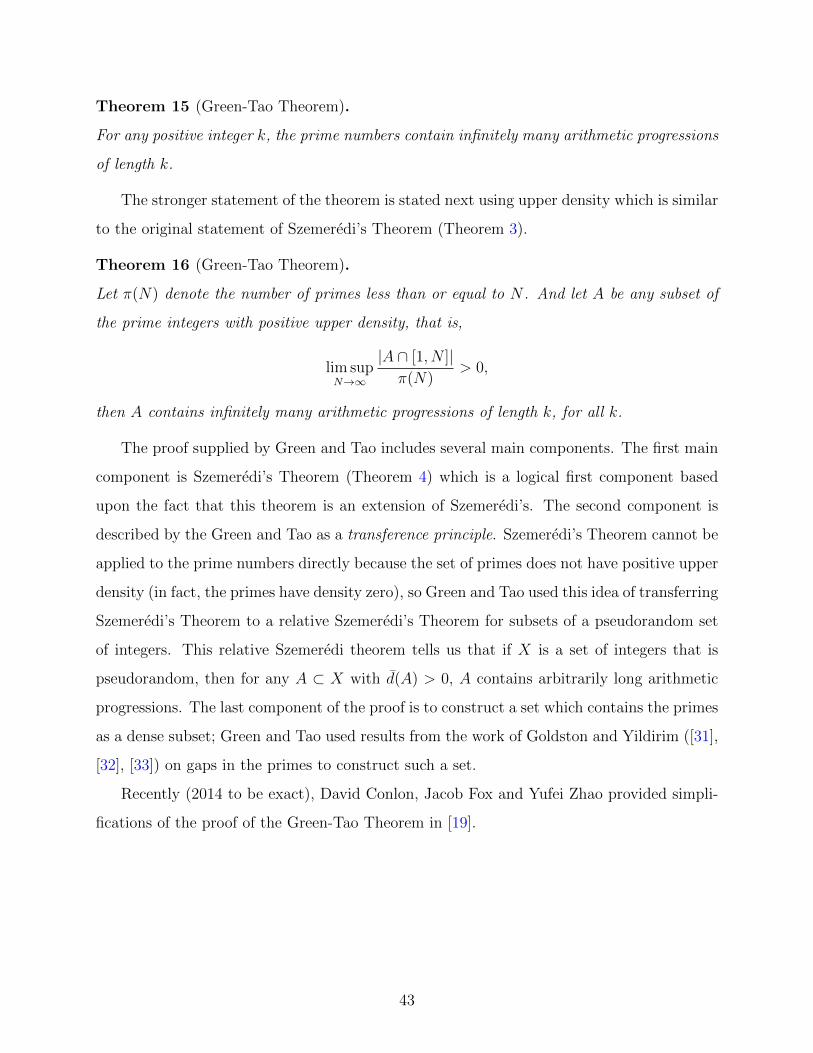
notably is the Green-Tao Theorem (Theorem 15) which we will discuss briefly in Section 5.6.
In a talk given in 1976 (and appearing in a book in 1977) Erdos expanded his original
conjecture on arithmetic progressions to the following conjecture:
Conjecture 1.
Let a1 < a2 < . . . be a sequence of integers such that∑
1ai
=∞, then the sequence contains
an arithmetic progression of arbitrary length.
Erdos offered $3000 for the proof of this conjecture, but never planned on having to pay
the reward due to the difficulty of the problem [24]. Erdos later raised the amount to $5000
and said he would leave money for the prize when he passed to be paid by Ronald Graham,
a longtime friend and fellow mathematician [48].
5
3.0 DEFINITIONS AND EXAMPLES
We begin by providing relevant definitions for our discussion and note that a primer on
graph theory is offered in the Appendix. For a more in-depth look at graph theory, refer
to [12] or [37]. Before we dive into the formal statement and applications of the Regularity
Lemma (Theorem 5), we need to define and understand several terms that our critical for
our discussion.
3.1 DENSITY
We begin with a simple definition of the density of a graph, more specifically, the density
between a pair of vertex subsets. We only consider simple graphs, that is, graphs with no
repeated edges or loops, and the majority of graphs considered in this paper will be dense
graphs meaning that the density is on the higher side and thus close to one. On the other
hand, a graph that is not dense is called sparse, and the density of a sparse graph is closer
to zero.
To determine whether a graph, G = (V,E), is dense or sparse, we must find the ratio
between the number of edges, |E|, and the maximum number of edges possible, 12|V |(|V |−1).
Definition 3 (Density of a Graph).
The density of a graph G, denoted d(G), is
d(G) =|E|
|V |(|V |−1)2
=2|E|
|V |(|V | − 1).
6
Complete graphs will always have a density of one, while a graph with no edges (an
empty graph) will have a density of zero, hence 0 ≤ d(G) ≤ 1.
Our discussion mainly requires the density between sets of vertices, hence the next defi-
nition.
Definition 4 (Density of a Pair of Vertex Subsets).
If G = (V,E) is a graph with X and Y nonempty, disjoint subsets of vertices, then the
density of the pair (X, Y ) is defined as
d(X, Y ) =e(X, Y )
|X||Y |,
where e(X, Y ) is the number of edges with one incident vertex in X and the other in Y .
Similar to the density of a graph, if a pair of sets of vertices does not have any edges
between them, then the density is 0. However, if every vertex of subset X is connected to
every vertex of subset Y , then e(X, Y ) = |X||Y | and the density of (X, Y ) is 1. Thus for
any pair (X, Y ), we have 0 ≤ d(X, Y ) ≤ 1.
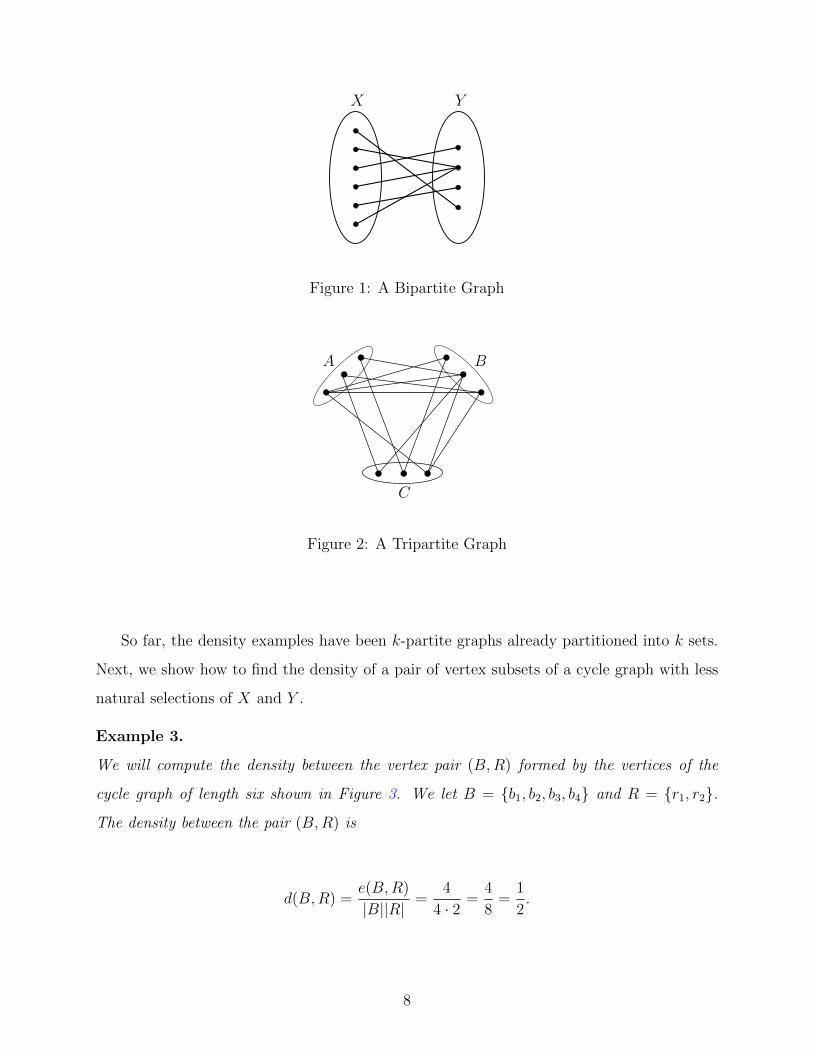
Example 1 and Example 2 show how to calculate the density of vertex pairs in a bipartite
graph (only one vertex pair to consider) and in a tripartite graph (three different pairs to
consider). Example 2 also finds the density of the tripartite graph itself.
Example 1.
To calculate the density of the pair in Figure 1, we note that we have 6 edges between the
sets X and Y . In addition, |X| = 6 and |Y | = 4. Thus,
d(X, Y ) =e(X, Y )
|X||Y |=
6
24=
1
4.
Example 2.
In the tripartite graph in Figure 2, we consider the pairs (A,B), (A,C), and (B,C). The
densities for each pair are:
d(A,B) =e(A,B)
|A||B|=
5
9; d(A,C) =
e(A,C)
|A||C|=
3
9=
1
3; d(B,C) =
e(B,C)
|B||C|=
4
9.
We can also calculate the density of the entire graph G: counting all of the edges gives 12
edges total and e(K9) = 36, so d(G) = 1236
= 13.
7
X Y
Figure 1: A Bipartite Graph
A B
C
Figure 2: A Tripartite Graph
So far, the density examples have been k-partite graphs already partitioned into k sets.
Next, we show how to find the density of a pair of vertex subsets of a cycle graph with less
natural selections of X and Y .
Example 3.
We will compute the density between the vertex pair (B,R) formed by the vertices of the
cycle graph of length six shown in Figure 3. We let B = {b1, b2, b3, b4} and R = {r1, r2}.
The density between the pair (B,R) is
d(B,R) =e(B,R)
|B||R|=
4
4 · 2=
4
8=
1
2.
8
b1 b2
b3 b4
r1 r2
(a) The Cycle Graph C6
b1
b2
b3b4
r1
r2
B R
(b) Vertex Pair (B,R)
Figure 3: The Cycle Graph C6 and Vertex Pair (B,R)
3.2 ε-REGULARITY
Szemeredi’s Regularity Lemma (Theorem 5) centers around vertex pairs that are ε-regular,
so it will be quite useful to understand what is meant by ε-regularity.
Definition 5 (ε-Regularity).
Let 0 < ε ≤ 1 be given and let G = (V,E) be a graph. For two disjoint non-empty sets of
vertices X and Y , the pair (X, Y ) is said to be ε-regular if for every A ⊆ X and B ⊆ Y
such that |A| ≥ ε|X| and |B| ≥ ε|Y |,
|d(A,B)− d(X, Y )| ≤ ε.
Thus, a pair (X, Y ) of subsets of vertices in a graph are ε-regular if big enough subsets of
X and Y have densities not very different from the density of (X, Y ). While we allow ε ≤ 1,
in that case that ε = 1, a vertex pair will always be ε-regular, so we are most interested in the
case when ε < 1. Note, if ε = 1, then the only subsets to consider are X and Y themselves
because we require A ⊆ X and |A| ≥ 1 · |X| which implies A = X and likewise B = Y .
If a pair does not meet this condition, we say the pair is ε-irregular . The following
examples demonstrate ε-regularity and ε-irregularity: in Example 4, we look at a pair that
9
does not meet the ε-regularity condition for a chosen ε; in Example 5, we consider a pair
that is ε-regular for some values of ε and ε-irregular for other values.
Example 4.
We will show that the pair (X, Y ) in Figure 4 is ε-irregular for a chosen positive ε < 1.
Note, d(X, Y ) = 34. In X, we have the three possible subsets as A1 = {x1}, A2 = {x2}, and
A3 = {x1, x2}. Similarly in Y , we have B1 = {y1}, B2 = {y2}, and B3 = {y1, y2}.
X Y
x1
x2
y1
y2
Figure 4: ε-Irregular Pair
Following the definition of ε-regularity, we find a working ε by comparing the cardinalities
of the subsets to the cardinalities of X and Y . For i = 1, 2, we have
|Ai| ≥ ε|X| =⇒ ε ≤ 1
2and |Bi| ≥ ε|X| =⇒ ε ≤ 1
2.
In addition,
|A3| ≥ ε|X| =⇒ ε ≤ 1 and |B3| ≥ ε|X| =⇒ ε ≤ 1.
We will show (X, Y ) is ε-irregular for 0 < ε ≤ 12. We must check that for at least one pair,
(Vi, Vj) such that 1 ≤ i ≤ 3 and 1 ≤ j ≤ 3, we have |d(Ai, Bj)− d(X, Y )| > 12.
The densities of the subsets are listed in Table 1. When i = 2 and j = 1, d(A2, B1) = 0
and so
|d(A2, B1)− d(X, Y )| = 3
4>
1
2
10
B1 B2 B3
A1 1 1 1
A2 0 1 12
A312
12
34
Table 1: Densities for subsets of irregular pair (X, Y )
which contradicts our choice of ε. Thus, (X, Y ) is 12-irregular and in fact, is ε-irregular for
all ε ≤ 12. Note that in general the same graph can be ε-regular for one ε, but ε-irregular for
a different ε. In this example, if ε > 12, the pair is regular because the only large subset to
consider would be the sets themselves and the difference between the densities is zero.
Example 5.
We will show that the pair (X, Y ) in Figure 5 is 12-regular; that is, for all |Ai| ≥ 1
2|X| and
|Bj| ≥ 12|Y |, we have |d(Ai, Bj)− d(X, Y )| ≤ 1
2. We have the subsets A1 = {x1}, A2 = {x2},
A3 = {x3}, A4 = {x1, x2}, A5 = {x1, x3}, A6 = {x2, x3} , and A7 = {x1, x2, x3} of the set
X, and we have the subsets B1 = {y1}, B2 = {y2}, B3 = {y3}, B4 = {y1, y2}, B5 = {y1, y3},
B6 = {y2, y3} , and B7 = {y1, y2, y3} of the set Y.
X Y
x1
x2
y1
y2
x3 y3
Figure 5: ε-Regular Pair
We only consider the subsets with cardinality greater than or equal to ε|X| = ε|Y | = 32, i.e.
11
subsets with two or three vertices. Note that we have |Ai| ≥ 32
and |Bi| ≥ 32
for 4 ≤ i, j ≤ 7.
Next, we compute the densities between each pair of subsets of X and Y which are stated in
Table 2. Note, d(X, Y ) = 69
= 23.
B4 B5 B6 B7
A434
34
12
23
A5 1 12
12
23
A634
34
12
23
A756
23
12
23
Table 2: Densities for subsets of regular pair (X, Y )
Then we compute the absolute values of the difference between the densities of the subsets
and the density of the pair.
|d(Ai, Bj)− d(X, Y )| =
0 if j = 7, and (i, j) = (7, 5)
112
if i = 4, 6 and j = 4, 5
16
if j = 6 and (i, j) = (5, 5) and (7, 4)
13
if i = 5 and j = 4
We can see that in all cases the absolute value of the difference between densities is less
than 12; hence, the pair in Figure 5 is 1
2-regular as desired.
Now that we understand what it means for a pair (X, Y ) to be ε-regular, we only need
a few more definitions. The first we consider is a particular partition of the vertices.
Definition 6 (Equipartition).
A vertex partition of disjoint sets V = V0 ∪ V1 ∪ V2 ∪ . . . ∪ Vk is called an equipartition if
|V1| = |V2| = . . . = |Vk| with V0 being the exceptional set.
12
Note the size of the exceptional set is allowed to differ from the size of the rest of the sets.
After the vertices of a graph are separated into k subsets of the same size, the remaining
(or leftover) vertices become elements of the exceptional set; this allows us to create an
equipartition of a graph of any size. Furthermore, the exceptional set is allowed to be empty
as well which is the case if k divides |V |.
Now, we combine the idea of an equipartition with the condition of ε-regularity to define
an ε-regular partition:
Definition 7 (ε-Regular Partition).
Let ε be fixed and let G = (V,E) be a graph. An equipartition V = V0 ∪ V1 ∪ . . . ∪ Vk is said
to be an ε-regular partition if |V0| ≤ ε|V | and at most εk2 pairs (Vi, Vj), which satisfy
1 ≤ i < j ≤ k, are ε-irregular.
An example of an ε-regular partition is included next.
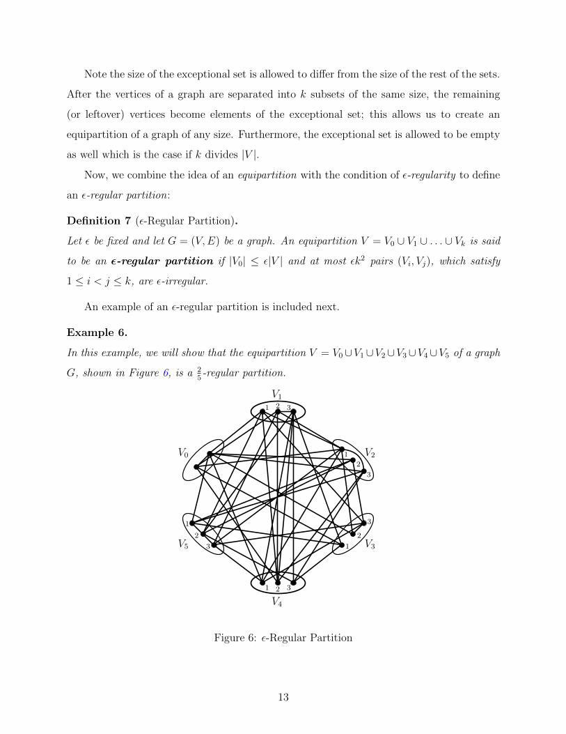
Example 6.
In this example, we will show that the equipartition V = V0∪V1∪V2∪V3∪V4∪V5 of a graph
G, shown in Figure 6, is a 25-regular partition.
V0
V11 2 3
V21
2
3
V3
3
2
1
V4
1 2 3
V5
1
2
3
Figure 6: ε-Regular Partition
13
First, we check 2 is less than 25· 17, which it is, to meet the condition that |V0| ≤ ε|V |.
The only other condition to meet to ensure that the equipartition is a 25-regular partition is
to determine how many 25-regular pairs exist in the partition. The partition must have less
than εk2 = 25· 52 = 10 irregular pairs to be a 2
5-regular partition.
Because ε = 25, we only consider subsets A of Vj (1 ≤ j ≤ 5) such that |A| ≥ 2
5|Vj| = 6
5.
Let Ai denote the subsets of V1, Bi denote the subsets of V2, Ci denote the subsets of V3, Di
denote the subsets of V4, and Fi denote the subsets of V5. Each Vi has seven subsets and the
subsets of V1 are the following:
A1 = {a1} A2 = {a2} A3 = {a3}
A4 = {a1, a2} A5 = {a1, a3} A6 = {a2, a3}
A7 = {a1, a2, a3}
We only consider the subsets numbered four through seven because the cardinality of
those subsets is greater that 65. Now, we must determine which of the ten pairs (Vi, Vj),
1 ≤ i < j ≤ 5, are 25-regular and which are 2
5-irregular. Table 3 lists the densities of the
subsets of V1, V2, V3, V4, and V5.
V1
V4(a) (V1, V4)
V1
V4(b) Subset of (V1, V4) with density zero.
Figure 7: (V1, V4) is an irregular pair
14
B4 B5 B6 B7 C4 C5 C6 C7 D4 D5 D6 D7 F4 F5 F6 F7
A412
12
0 13
0 14
14
16
12
0 12
13
14
14
12
13
A514
14
0 16
14
12
14
13
34
12
34
23
12
14
12
13
A614
14
0 16
14
14
0 16
12
12
34
23
14
14
12
13
A713
13
0 29
16
13
16
29
23
13
23
59
13
16
12
13
B414
14
12
13
14
14
0 16
12
12
12
12
B514
0 14
16
12
12
12
12
14
12
14
13
B6 0 14
14
16
14
14
12
13
34
12
14
12
B716
16
13
29
13
13
13
13
12
12
13
49
C4 0 14
14
16
14
14
0 16
C514
12
14
13
14
12
14
13
C614
14
0 16
0 14
14
16
C716
13
16
29
16
13
16
29
D4 0 14
14
16
D514
14
12
13
D614
14
14
16
D716
16
13
29
Table 3: Densities for subsets of V1, V2, V3, V4, and V5
The 25-regular pairs are (V1, V2), (V1, V3), (V1, V5), (V2, V3), (V2, V4), (V2, V5), (V3, V4),
(V3, V5), and (V4, V5). The only 25-irregular pair is (V1, V4).
From Figure 7a, we find d(V1, V4) = 59. If we consider the subsets containing the vertices
highlighted in red in Figure 7b (which corresponds to the subsets A4 and D5), then from Table
3, d(A4, D5) = 0. Then
|d(A4, D5)− d(V1, V4)| =5
9>
2
5
which implies (V1, V4) is an irregular pair.
15
Because the size of the exceptional set and the number of irregulars pairs are both bounded,
the equipartition in Figure 6 is a 25-regular partition as desired.
3.3 INDEX OF A PARTITION
We have stated the definitions that are needed for the formal statement of the Regularity
Lemma and now state two definitions which are needed for other parts of this paper. The
first will be needed for the proof of the Regularity Lemma (Theorem 5). The index is the
mean square density of P (as noted in [6]) and is a measure of how regular a partition is.
Definition 8 (Index).
If V = V0 ∪ V1 ∪ V2 ∪ . . . ∪ Vk is an equipartition of a graph G, then we define the index of
V as
ind(V ) =1
k2
k∑i=1
k∑j=i+1
[d(Vi, Vj)]2
Recall, d(Vi, Vj) ≤ 1 for any pair of vertex subsets. Therefore, we see that for any V
ind(V ) ≤ 1
k2
k∑i=1
k∑j=i+1
1 =1
k2
k∑i=1
(k − i) =1
k2· 1
2k(k − 1) =
k − 1
2k<
1
2.
3.4 REDUCED GRAPH
Our last definition is needed in a few of the applications that we will discuss later in the
paper. In the chapter of applications (Chapter 5), one technique using the Regularity Lemma
is to create a reduced graph.
Definition 9 (Reduced Graph).
Given a graph G = (V,E) and an ε-regular partition P = V0 ∪ V1 ∪ . . . ∪ Vk of V , such that
|V1| = . . . = |Vk| = `, the reduced graph, R, is the graph formed by vertices V1, V2, . . . , Vk
such that ViVj is an edge if the pair (Vi, Vj) is a ε-regular pair with density at least d ∈ (0, 1].
We may also denote the reduced graph R as the (ε, d)-reduced graph.
16
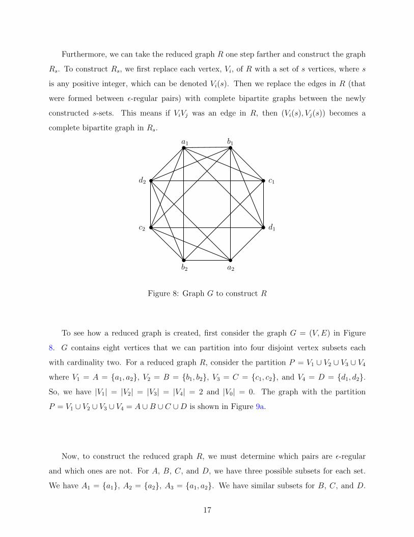
Furthermore, we can take the reduced graph R one step farther and construct the graph
Rs. To construct Rs, we first replace each vertex, Vi, of R with a set of s vertices, where s
is any positive integer, which can be denoted Vi(s). Then we replace the edges in R (that
were formed between ε-regular pairs) with complete bipartite graphs between the newly
constructed s-sets. This means if ViVj was an edge in R, then (Vi(s), Vj(s)) becomes a
complete bipartite graph in Rs.
a1
a2b2
b1
c1
d1c2
d2
Figure 8: Graph G to construct R
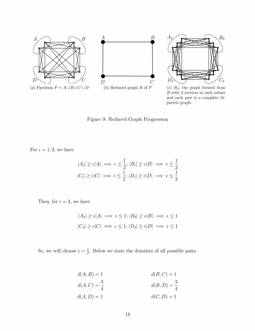
To see how a reduced graph is created, first consider the graph G = (V,E) in Figure
8. G contains eight vertices that we can partition into four disjoint vertex subsets each
with cardinality two. For a reduced graph R, consider the partition P = V1 ∪ V2 ∪ V3 ∪ V4where V1 = A = {a1, a2}, V2 = B = {b1, b2}, V3 = C = {c1, c2}, and V4 = D = {d1, d2}.
So, we have |V1| = |V2| = |V3| = |V4| = 2 and |V0| = 0. The graph with the partition
P = V1 ∪ V2 ∪ V3 ∪ V4 = A ∪B ∪ C ∪D is shown in Figure 9a.
Now, to construct the reduced graph R, we must determine which pairs are ε-regular
and which ones are not. For A, B, C, and D, we have three possible subsets for each set.
We have A1 = {a1}, A2 = {a2}, A3 = {a1, a2}. We have similar subsets for B, C, and D.
17
A B
CD
(a) Partition P = A∪B ∪C ∪D
A B
CD(b) Reduced graph R of P
A3 B3
C3D3
(c) R3, the graph formed fromR with 3 vertices in each subsetand each pair is a complete bi-partite graph.
Figure 9: Reduced Graph Progression
For i = 1, 2, we have
|Ai| ≥ ε|A| =⇒ ε ≤ 1
2; |Bi| ≥ ε|B| =⇒ ε ≤ 1
2
|Ci| ≥ ε|C| =⇒ ε ≤ 1
2; |Di| ≥ ε|D| =⇒ ε ≤ 1
2
Then, for i = 3, we have
|A3| ≥ ε|A| =⇒ ε ≤ 1; |B3| ≥ ε|B| =⇒ ε ≤ 1
|C3| ≥ ε|C| =⇒ ε ≤ 1; |D3| ≥ ε|D| =⇒ ε ≤ 1
So, we will choose ε = 12. Below we state the densities of all possible pairs.
d(A,B) = 1 d(B,C) = 1
d(A,C) =3
4d(B,D) =
3
4
d(A,D) = 1 d(C,D) = 1
18
B1 B2 B3 C1 C2 C3 D1 D2 D3
A1 1 1 1 1 1 1 1 1 1
A2 1 1 1 0 1 12
1 1 1
A3 1 1 1 12
1 34
1 1 1
B1 1 1 1 1 1 1
B2 1 1 1 0 1 12
B3 1 1 1 12
1 34
C1 1 1 1
C2 1 1 1
C3 1 1 1
Table 4: Densities for subsets of A, B, C, and D
Next, we want to determine which pairs are 12-regular and which pairs are 1
2-irregular.
Recall we are checking if the difference between the densities of the sets and densities of the
subsets are less than or equal to 12. Utilizing the values in Table 4, for 1 ≤ i, j ≤ 3, we have
the following:
|d(Ai, Bj)− d(A,B)| ≤ 1
2|d(Ai, Dj)− d(A,D)| ≤ 1
2
|d(Bi, Cj)− d(B,C)| ≤ 1
2|d(Ci, Dj)− d(C,D)| ≤ 1
2
However, for the pairs (A,C) and (B,D), we have specific values of i and j such that
|d(A2, C1)− d(A,C)| > 1
2and |d(B3, D1)− d(B,D)| > 1
2.
From our calculations, the regular pairs are (A,B), (A,D), (B,C), and (C,D) while the
irregular pairs are (A,C) and (B,D).
19
By the definition of a reduced graph, there must be an ε-regular partition which means
we need to check that we have at most εk2 irregular pairs. From our calculations above, we
have four regular pairs and two irregular pairs. We have ε = 12
and k = 4, so εk2 = 12(42) = 8.
So, we meet the condition on the number irregular pairs. Also, we must have |V0| ≤ ε|V |
and we meet this condition immediately because |V0| = 0. So, our partition P is an ε-regular
partition with ε = 12.
We are now ready to construct the reduced graph R, shown in Figure 9b, by replacing
each vertex set with a single vertex and constructing an edge wherever there is a regular
pair. Because we have 4 vertex sets, we have 4 vertices in R and because the regular pairs
are (A,B), (B,C), (C,D), and (A,D), we construct the edges AB, BC, CD, and AD.
Furthermore the pairs (A,C) and (B,D) are irregular, so we do not construct edges between
these pairs.
The last step is to construct Rs from R for some positive integer s. For our example, we
will replace each vertex with a set of three vertices. So, the vertex A in R will become a set
of three vertices denoted A3. We replace B, C, and D similarly with sets of three vertices
denoted B3, C3, and D3. The next step is to replace each edge by a complete bipartite graph
between the vertex sets. For example, the edge AB becomes a complete bipartite graph
between A3 and B3 with nine edges. The graph R3 can been seen in Figure 9c. Going from
R to Rs, we could have chosen any positive integer for s and the process would have been
the same. However, for demonstration purposes, s = 3 was a manageable integer.
20
4.0 FORMAL STATEMENT AND PROOF
Equipped with the relevant definitions, we are ready to formally state the Szemeredi Reg-
ularity Lemma. Recall we stated that the lemma roughly states that dense graphs can be
approximated by random graphs. Naturally, we want to see what this looks like mathemat-
ically.
Theorem 5 (Szemeredi’s Regularity Lemma).
For every ε ∈ (0, 1] and m > 0, there exist integers N and M = M(m, ε) such that for every
n ≥ N , every graph G = (V,E) with n vertices has an ε-regular partition V = V0∪V1∪. . .∪Vk,
which satisfies m ≤ k ≤M.
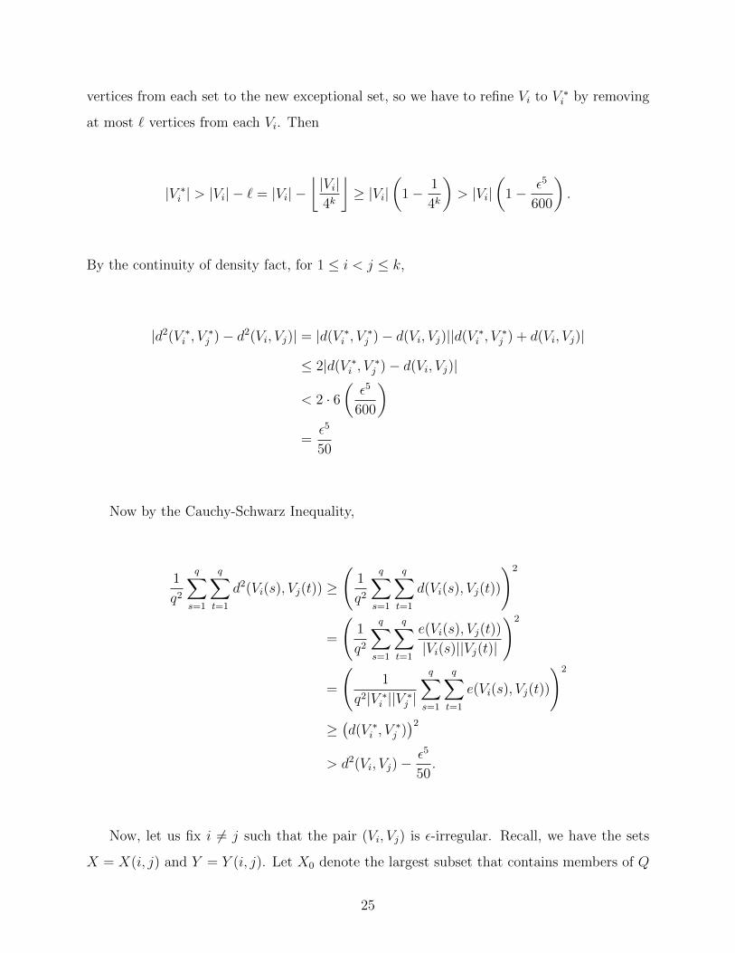
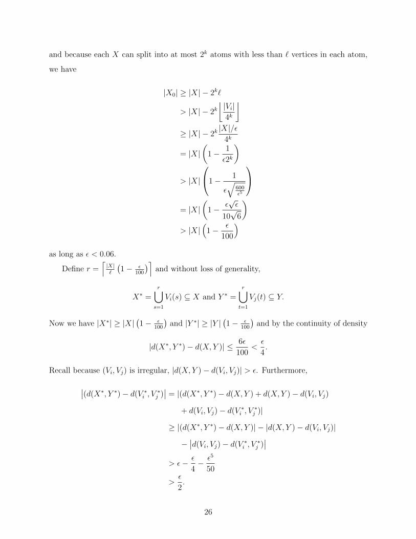
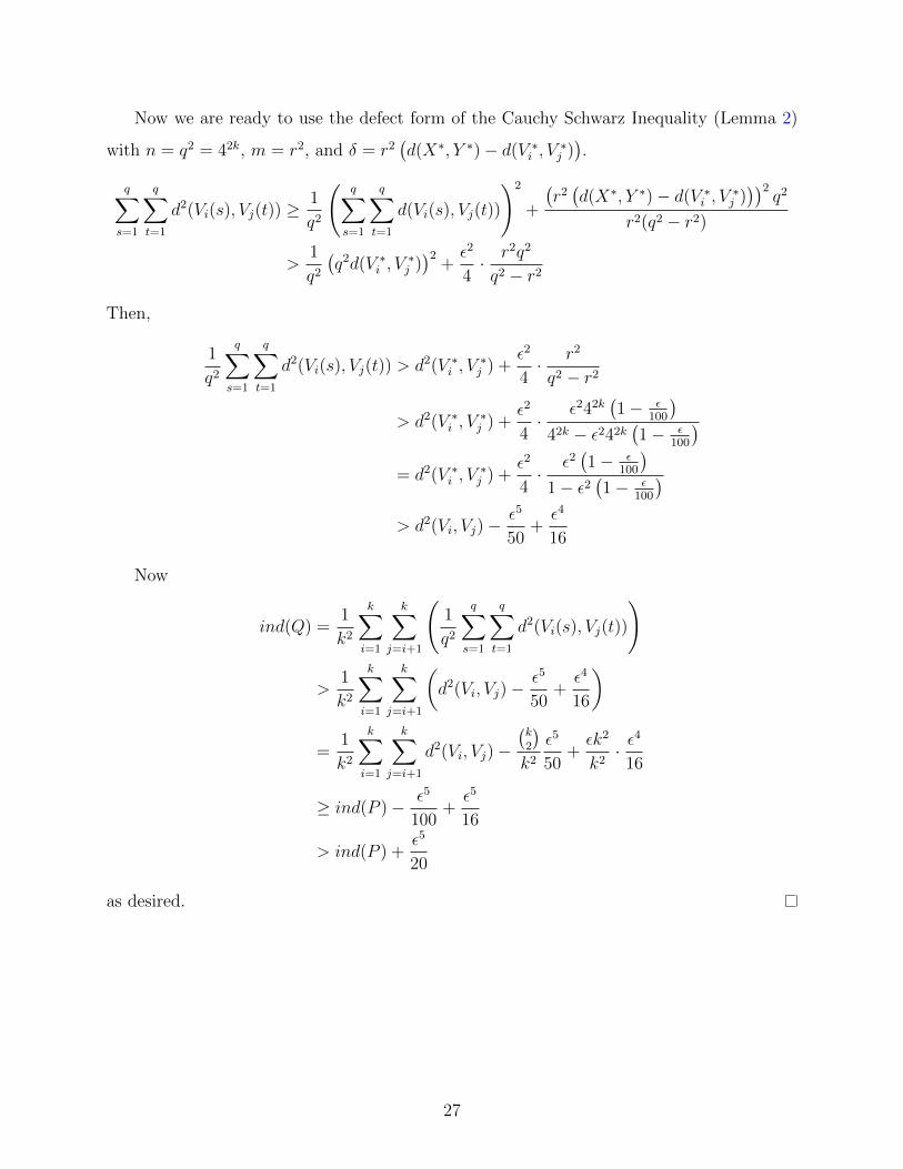
Following Szemeredi’s approach in [50], we need one main lemma in order to prove the
Regularity Lemma. We will discuss the proof of Lemma 1 after the proof of the Regularity
Lemma.
Lemma 1.
Let G = (V,E) be a graph with n vertices. We let P be an equipartition of V into classes
V0 ∪ V1 ∪ V2 ∪ . . . ∪ Vk, where V0 is the exceptional class. Let 0 < ε ≤ 1 be given such that
4k > 600ε−5. If more than εk2 pairs are ε-irregular, then there exists an equipartition Q of V
into 1 + k4k classes such that the size of the exceptional class increases by at most n4k
, that
is, |Q0| ≤ |V0|+ n4k
and
ind(Q) > ind(P ) +ε5
20.
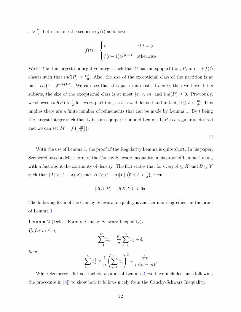
Proof of Theorem 5. Let s be the smallest integer such that 4s > 600ε−5, where s > m and
21
s > 2ε. Let us define the sequence f(t) as follows:
f(t) =
s if t = 0
f(t− 1)4f(t−1) otherwise
We let t be the largest nonnegative integer such that G has an equipartition, P , into 1+f(t)
classes such that ind(P ) ≥ tε5
20. Also, the size of the exceptional class of the partition is at
most εn(1− 2−(t+1)
). We can see that this partition exists if t = 0, then we have 1 + s
subsets, the size of the exceptional class is at most ε2n < εn, and ind(P ) ≥ 0. Previously,
we showed ind(P ) < 12
for every partition, so t is well defined and in fact, 0 ≤ t < 10ε5
. This
implies there are a finite number of refinements that can be made by Lemma 1. By t being
the largest integer such that G has an equipartition and Lemma 1, P is ε-regular as desired
and we can set M = f(⌊
10ε5
⌋).
With the use of Lemma 1, the proof of the Regularity Lemma is quite short. In his paper,
Szemeredi used a defect form of the Cauchy-Schwarz inequality in his proof of Lemma 1 along
with a fact about the continuity of density. The fact states that for every A ⊆ X and B ⊆ Y
such that |A| ≥ (1− δ)|X| and |B| ≥ (1− δ)|Y |(0 < δ < 1
3
), then
|d(A,B)− d(X, Y )| < 6δ.
The following form of the Cauchy-Schwarz Inequality is another main ingredient in the proof
of Lemma 1.
Lemma 2 (Defect Form of Cauchy-Schwarz Inequality).
If, for m ≤ n,m∑k=1
xk =m
n
n∑k=1
xk + δ,
thenn∑k=1
x2k ≥1
n
(n∑k=1
xk
)2
+δ2n
m(n−m).
While Szemeredi did not include a proof of Lemma 2, we have included one (following
the procedure in [6]) to show how it follows nicely from the Cauchy-Schwarz Inequality.
Concordia University in Montreal, Canada as the Canada Research Chair in combinatorial
optimization and then discrete mathematics before retiring in 2014. His research interest be-
gan in graph theory and combinatorics, spending about 17 years on the Traveling Salesman
Problem, then he worked in analysis of algorithms and operations research before developing
an interest in computational neurosience. One of his well known results is the art gallery
theorem. The original art gallery problem was posed to determine the minimum number of
guards needed to guard an art gallery such that the entire art gallery can be observed by the
guards. Chvatal gave an upper bound stating that⌊n3
⌋will always be a sufficient number of
guards [15].
Pal Erdos
Pal (Paul) Erdos was born on March 26, 1913 in Budapest, Austria-Hungary and is consid-
ered one of most prolific mathematicians of all time. From an early age, he showed great
mathematical ability; by the age of four, he could multiple three digit integers and under-
stand the idea of negative integers. He received his Ph.D. from Peter Pazmany University
in Budapest (now Eotvos Lorand University of Budapest) in 1934 at the age of 21.
At the start of his career, Erdos took a postdoctoral position at the University of Manch-
ester for four years before moving to the United States to work at the Institute for Advanced
Study at Princeton University for a year. This was the start of his nomadic life; he opted to
travel from one university to another to collaborate with whomever he wished without being
tied down to just one university. This lead to Erdos collaborating with over 500 mathemati-
cians [2] and publishing over 1500 papers in his lifetime [3]. To pay tribute to the number
of mathematicians Erdos collaborated with, his friends created the Erdos number, a number
assigned to a mathematician to determine the distance from Erdos to the mathematician
through collaborations. Erdos has an Erdos number of 0, the over 500 mathematicians who
have co-written a paper with Erdos have an Erdos number of 1, those who have co-written
with a co-author of Erdos have an Erdos number of 2, and so on. If there is no path of papers
between Erdos and a mathematician, the mathematician has an Erdos number of infinity.
He was awarded the Wolf Prize in Mathematics in 1983/4 for his contributions in number
theory, combinatorics, set theory, mathematical analysis, and probability as well as encour-
45
aging other mathematicians. One way in which Erdos stimulated other mathematicians was
by offering prize money for proofs (or disproofs) of problems that he himself could not solve
with the amount of the award being based upon the difficulty of the problem according to
Erdos. The amount would range from around $10 to several thousands of dollars. After his
death in 1996, his close friends Ronald Graham and Fan Chung (both mathematicians them-
selves and collaborators of Erdos’) announced they would continue to award prize money for
the Erdos problems in graph theory which can be found in the book they published detailing
the unsolved problems [13].
When referring to someone who had passed away, Erdos would say they had “left” while
someone who “died” was someone who had stopped doing mathematics. Erdos lived until
the age of 83 when he left on September 20, 1996 due to suffering a heart attack while
attending a conference in Warsaw, Poland.
Ben Green
Ben Green was born on February 27, 1977 in Bristol, England and earned his Ph.D. from
the University of Cambridge under the supervision of Timothy Gowers. He is currently
the Waynflete Professor of Pure Mathematics at the University of Oxford; the Waynflete
Professorship is one of four professorial fellowships at the University of Oxford. Green works
in the area of additive combinatorics and one of his well known results is his theorem with
Terrence Tao on arithmetic progression in the primes (see Section 5.6).
Frank Ramsey
Frank Ramsey was born on February 22, 1903 in Cambridge, England and unfortunately
had quite a short life before passing on January 19, 1930. However, he was able to influence
mathematics in those short 26 years. He received his Bachelor’s degree from Trinity College.
Along with his work in mathematics, he was also a philosopher and an economist. He began
teaching in 1926 as a lecturer at King’s College and later became the Director of Studies in
Mathematics. His second paper in mathematics titled On a problem of formal logic is what
started the area of Ramsey Theory (Section 5.4) [46].
46
Miklos Simonovits
Miklos Simonovits was born in September 4, 1943 in Budapest, Hungary. He earned his
Ph.D. in 1971 from Eotvos Lorand University of Budapest under the supervision of Vera
Sos. His main areas of research are extremal graph theory, theoretical computer science, and
random graphs. As of 1979, he is a part of the Alfred Renyi Insitute of Mathematics. He
has an Erdos number of 1 having worked with Erdos on twenty one papers. In 2014, he was
awarded the Szechenyi Prize, an award given by the government of Hungary to recognize
scientists’ contributions to academia in the country; in fact, Simonovits’ advisor Sos was also
awarded the prize in 1997.
Vera T. Sos
Vera Sos was born on September 11, 1930 in Budapest, Hungary. While still an undergrad-
uate at Eotvos Lorand University of Budapest, she began teaching at the school in 1950.
Then, she graduated in 1952, married Pal Turan, and began her graduate studies; she was
awarded her Ph.D. from the Hungarian Academy of Sciences in 1957. Since 1987, she has
been a professor at Alfred Renyi Institute of Mathematics, Hungarian Academy of Science.
Sos is known for her work in number theory and combinatorics. She collaborated with Erdos
on thirty five papers giving her an Erdos number of 1.
Arthur Stone
Arthur Harold Stone was born on September 30, 1916 in London, England. He received his
Ph.D. from Princeton University in 1941 and worked mostly in the discipline of topology.
His wife, Dorothy Maharam, was also a mathematician working in the field of measure
theory. They both were professors for many years at the University of Rochester with
Stone becoming professor emeritus in 1987 upon his retirement. He continued teaching at
Northwestern University as an adjunct professor until his passing in 2000.
Endre Szemeredi
Endre Szemeredi was born on August 21, 1940 in Budapest, Hungary. Before becoming a
mathematician, Szemeredi went to medical school because his parents wanted him to be a
doctor. He left after several months when he decided he did not want to be a doctor and the
47
profession was not for him. He completed his Master’s degree at Eotvos Lorand University of
Budapest before earning his Ph.D. in 1970 at Moscow State University. His advisor was Israel
Gelfand, but Szemeredi had originally intended on studying under Alexander Gelfond and
unfortunately misspelled Gelfond’s name on his application which resulted in him becoming
Gelfand’s student. As of 1986, Szemeredi is a Professor of Computer Science at Rutgers
University in New Jersey and he is also a reseach fellow at the Alfred Renyi Institute of
Mathematics. He is well known for his proof of a conjecture from Erdos and Turan known as
Szemeredi’s Theorem (Theorem 4) [49] and his Regularity Lemma (Theorem 5) [50]. In 2012,
he received the Abel Prize, one of the top prizes in mathematics, for his work in discrete
mathematics and theoretical computer science.
Terence Tao
Terence Tao was born on July 17, 1975 in Adelaide, Australia and showed extraordinary
mathematical ability from an early age, eventually earning the nickname the Mozart of
Math. He completed his Bachelor’s degree at age 16 and his Master’s degree at age 17. Tao
applied to Princeton University with a letter of recommendation from Erdos, was accepted,
and earned his Ph.D. when he was only 20 years old. He immediately joined the faculty at
UCLA before being appointed to full professor when he was 24 years old. While he knew
Erdos, they never wrote a paper together, but Tao does have an Erdos number of 2. In 2006,
Tao was awarded the Fields Medal: one of the highest honors in mathematics. The Fields
Medal is only awarded once every four years to either two, three, or four mathematicians
under the age of 40 for their contributions to mathematics and for their potential of future
achievements. Tao also received one of the 2015 Breakthrough Prizes in Mathematics worth
three million dollars [44]. The Breakthrough Prize in Mathematics was announced in 2013,
with the first prize being awarded in 2015, and funded by Yuri Milner and Facebook founder
Mark Zuckerberg.
Pal Turan
Pal (Paul) Turan was born on August 18, 1910 in Budapest, Hungary. He received his Ph.D.
in 1935 from Eotvos Lorand University of Budapest. Because of his Jewish heritage, it was
difficult to find a job, but he was able to take a teaching position in 1938 before being send
48
to labor service between the years 1940 and 1944. In 1945, he was hired at Eotvos Lorand
University and became a full professor in 1949. He worked for many years before eventually
passing in 1976 as a result of leukemia. His work was mainly in the area of number theory,
but he worked in analysis and graph theory as well. In graph theory, he is known for founding
extremal graph theory with his theorem (Theorem 8). Some regard his power sum method
as his most well known achievement [38]; the power sum method provides lower bounds
for power sums and was discovered by Turan while he was investigating zeros of the zeta
function.
Bartel Leendert van der Waerden
B.L. van der Waerden was born on February 2, 1903 in Amsterdam, Netherlands. His father
was a mathematics teacher, but as a young child, van der Waerden was not allowed to read
his father’s math books but rather was encouraged to play outside [1]. This only made van
der Waerden more curious about mathematics and led him to receiving his Ph.D. from the
University of Amsterdam in 1926 at the age of 23. He began teaching at the University of
Groningen before going to the University of Leipzig in 1931, but was forced to leave due to
the bombing of Leipzig the night of December 4, 1943. Eventually, he went to the University
of Zurich for the remainder of his career. He retired in 1973 and passed on January 12, 1996.
He is known for his work in abstract algebra, but he also worked in the areas of algebraic
geometry, quantum mechanics (he worked with Werner Heisenberg in Leipzig), and more.
49
7.0 CONCLUSION
We have seen that Szemeredi’s Regularity lemma is a deep result with applications in nu-
merous disciplines of mathematics. What began as a lemma in another theorem has become
a celebrated result in graph theory.
Whether we are removing edges from a graph, embedding graphs and trees, or proving
there exist arithmetic progressions in sets of the integers, the Regularity Lemma gives us a
starting point. The lemma allows us to know how the edges of a graph are distributed over
a partition of the vertices whereas without the lemma we may not know anything about a
given graph.
Szemeredi’s Regularity Lemma continues to be a frequently used theorem in graph theory
as we saw with the work on the approximate version of the Loebl-Komlos-Sos Conjecture [43].
Furthermore, there is unpublished work that is in preparation of a proof of the Erdos-Sos
Conjecture for large trees that utilizes the Regularity Lemma as well [4].
This paper is only an introduction to the complexity and reach of the Regularity Lemma
discussing the basic information to understand the lemma and a few of the numerous appli-
cations, but now we have a little bit more knowledge of this truly amazing result.
50
APPENDIX
A GRAPH THEORY PRIMER
For those who may not be as familiar with graph theory, this appendix is provided as a short
crash course in basic material needed for our discussion. The first part of the Appendix will
go through the basic definitions associated with graphs, then we will have a short discussion
on trees.
In order to study graph theory, we must first know how a graph is defined. A graph
is an ordered pair, which we shall denote as G = (V,E), where V is a nonempty set of
objects called vertices and E is a set of objects called edges. We can also denote the set of
vertices of G as v(G) and the set of edges of G as e(G). An edge is an unordered pair of
distinct vertices. Vertices connected by an edge are called adjacent vertices . Furthermore,
if vertices a and b are connected by the edge e, we say a and e are incident as well as b and
e are incident. In addition, we can say that a is an incident vertex of e and similarly for b.
One may be interested in the degree of a vertex which is the number of edges incident to a
particular vertex. Let v ∈ V be a vertex of G, then the degree of v is denoted deg(v).
If every unique edge connects a pair of distinct vertices, we refer to this graph as complete,
as seen in Figure 14. We denote a complete graph by Kr, where r is the number of vertices.
Another way to think about a complete graph is that if G has n vertices, then for every
vi ∈ V , i = 1, 2, . . . , n, deg(vi) = n− 1.
For our discussion, we will be considering simple graphs unless otherwise stated. A simple
graph is a graph with no repeated edges or loops. A loop is an edge that only has one vertex,
meaning the loop connects a vertex to itself.
51
Figure 14: The Complete Graph K6
We say a graph is k-partite (k ≥ 1) if the set V can be partitioned into k subsets
V1, V2, . . . , Vk such that every edge connects a vertex from Vi to a vertex in Vj such that
i 6= j. Thus, there does not exist any edges between vertices in the same subset. When
k = 2 and k = 3, we refer to this as a bipartite graph and tripartite graph, respectively.
Now that we have a basic understanding of graphs, we continue with a brief discussion
of trees. A tree is a connected acyclic graph. See Figure 16 for an example of trees. As a
reminder, a connected graph is a graph in which there is a path between any two vertices.
This means that we can reach any vertex from any of the remaining vertices by a series of
edges. Also, an acyclic graph is a graph that does not contain any graph cycles.
v1 v2
v3v4
v5
Figure 15: Cyclic Graph
To define a cycle, let us also consider a walk and a path. These terms are used for all
graphs, however, for our discussion, it is only relevant for trees. Given two vertices u and v
52
in a graph G, a u-v walk is a finite and alternating sequence of vertices and edges beginning
with u and ending with v. Furthermore, if u = v, that is, the walk begins and ends with u,
then we classify the walk as a closed walk . In Figure 15, W1 : v1, V5, v3, v1, v2 is a walk and
W2 : v5, v2, v3, v5 is a closed walk. Note, we may repeat vertices and edges in a walk.
A path, which can also be called a u-v path, is a walk in which no vertex is repeated. For
example, in Figure 15, W3 : v1, v2, v5, v4 is a path. We can relate walks and paths because
every path is a walk but the converse, that every walk is a path, is not necessarily true.
Finally, a cycle is a u-v walk in which u = v and no vertex is repeated. Another way
to think of a cycle is a closed path, or a closed walk with all distinct vertices. Figure 15 is
a cyclic graph because it contains at least one cycle. For example, W4 : v1, v2, v3, v4, v1 is a
cycle.
Now, back to trees. It may be interesting to note that all acyclic graphs (and therefore,
all trees) are bipartite. Figure 17 shows the trees from Figure 16 as bipartite graphs.
Figure 16: All trees of order 5.
Figure 17: All trees of order 5 shown as bipartite graphs.
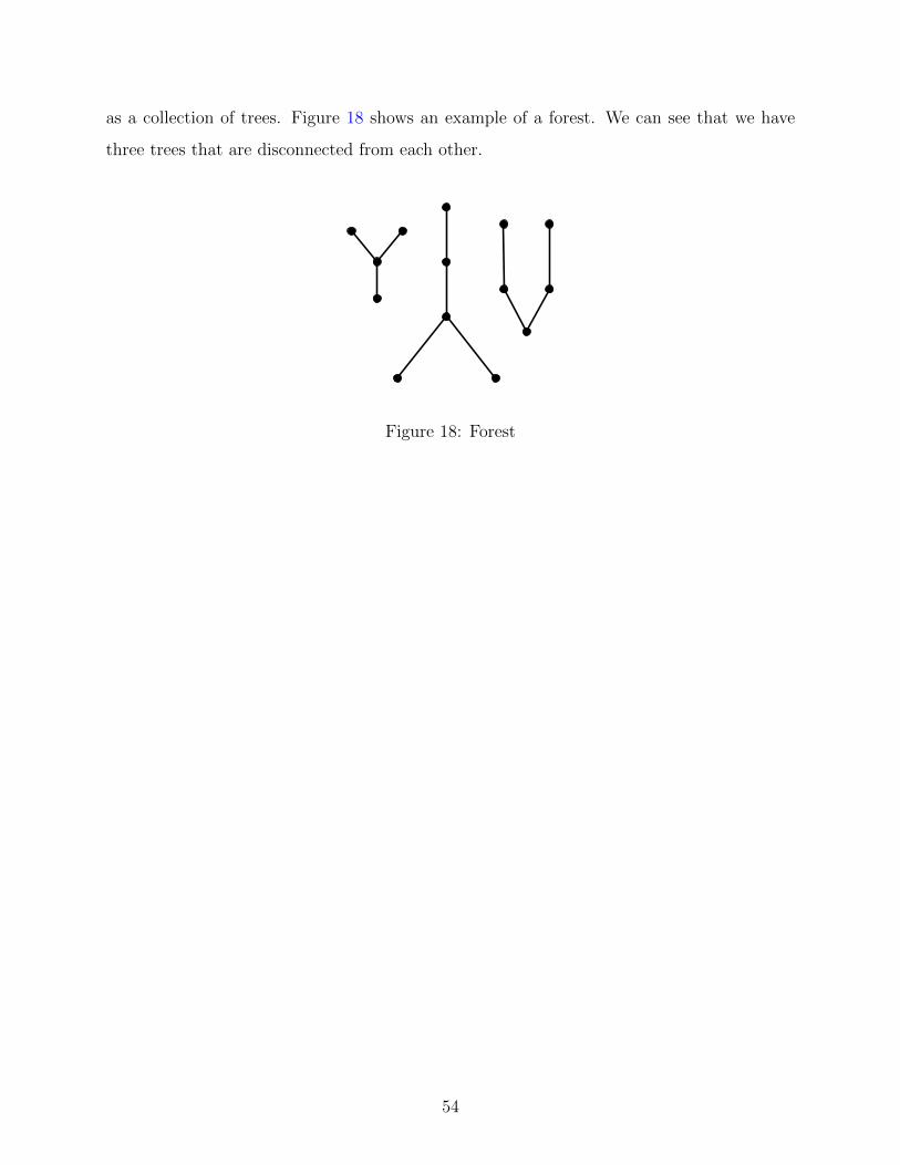
If a graph G is acyclic and disconnected, then G is a forest . A forest can be thought of
53
as a collection of trees. Figure 18 shows an example of a forest. We can see that we have
three trees that are disconnected from each other.
Figure 18: Forest
54
BIBLIOGRAPHY
[1] http://www-history.mcs.st-andrews.ac.uk/Biographies/Van der Waerden.html.Accessed: 2017-04-17.
[2] List of Erdos Coauthors. http://www.ams.org/mathscinet/MRAuthorID/189017. Ac-cessed: 2017-04-20.
[3] List of Erdos Publications. https://oakland.edu/enp/pubinfo/. Accessed: 2017-04-20.
[4] Ajtai, M., Komlos, J., Simonovits, M., and Szemeredi, E. Proof of the Erdos-Sos Conjecture for large trees. In preparation.
[5] Bollobas, B. Extremal graph theory. Courier Corporation, 2004.
[6] Bollobas, B. Modern graph theory, vol. 184. Springer Science & Business Media,2013.
[7] Bollobas, B., and Erdos, P. On the Structure of Edge Graphs. Bulletin of theLondon Mathematical Society 5, 3 (1973), 317–321.
[8] Bollobas, B., Erdos, P., and Simonovits, M. On the Structure of Edge GraphsII. Journal of the London Mathematical Society s2-12, 2 (1976), 219–224.
[9] Bollobs, B. Random Graphs, 2 ed. Cambridge Studies in Advanced Mathematics.Cambridge University Press, 2001.
[10] Brown, W. G., Erdos, P., and Sos, V. T. Some extremal problems on r-graphs. InNew directions in the theory of graphs (Proc. Third Ann Arbor Conf., Univ. Michigan,Ann Arbor, Mich, 1971) (1973), Academic Press, New York, pp. 53–63.
[11] Burr, S. A., and Erdos, P. On the magnitude of generalized Ramsey numbers forgraphs. In Infinite and finite sets (Colloq., Keszthely, 1973; dedicated to P. Erdos on his60th birthday), Vol. 1 (1975), North-Holland, Amsterdam, pp. 215–240. Colloq. Math.Soc. Janos Bolyai, Vol. 10.
[12] Chartrand, G. Introduction to graph theory. Tata McGraw-Hill Education, 2006.
[13] Chung, F., and Graham, R. Erdos on Graphs: His Legacy of Unsolved Problems.Ak Peters Series. Taylor & Francis, 1998.
[14] Chvatal, V. Some unknown van der waerden numbers. Combinatorial Structures andtheir Applications (1970), 31–33.
[15] Chvatal, V. A combinatorial theorem in plane geometry. Journal of CombinatorialTheory, Series B 18, 1 (1975), 39–41.
[16] Chvatal, V., Rodl, V., Szemeredi, E., and Trotter, W. The Ramsey numberof a graph with bounded maximum degree. Journal of Combinatorial Theory, Series B34, 3 (1983), 239 – 243.
[17] Chvatal, V., and Szemeredi, E. On the Erdos-Stone theorem. Journal of theLondon Mathematical Society s2-23, 2 (1981), 207–214.
[18] Conlon, D., and Fox, J. Graph removal lemmas. Surveys in combinatorics 1, 2(2013), 3.
[19] Conlon, D., Fox, J., and Zhao, Y. The green-tao theorem: an exposition. arXivpreprint arXiv:1403.2957 (2014).
[20] Das, S. Applications of the Szemeredi Regularity Lemma. Available at http:
[21] DESKUS, C. An Introduction To The Regularity Lemma. Available athttp://www.math.uchicago.edu/~may/VIGRE/VIGRE2011/REUPapers/Deskus.pdf(2016/10/06).
[22] Diestel, R. Graph Theory. Graduate Texts in Mathematics. Springer New York, 2000.
[23] Erdos, P. Extremal problems in graph theory. In Theory of Graphs and its Applica-tions, Proc. Sympos. Smolenice (1964), pp. 29–36.
[24] Erdos, P. Problems in number theory and combinatorics. In Proceedings of the sixthManitoba Conference on Numerical Mathematics (1977), pp. 35–58.
[25] Erdos, P., Furedi, Z., Loebl, M., and Sos, V. T. Discrepancy of trees. StudiaSci. Math. Hungar. 30, 1-2 (1995), 47–57.
[26] Erdos, P., and Simonovits, M. A limit theorem in graph theory. Studia ScientiarumMathematicarum Hungarica 1 (1965), 51–57.
[27] Erdos, P., and Stone, A. H. On the Structure of Certain Graphs. Bulletin of theAmerican Mathematical Society 28 (1946), 1087–1091.
[28] Erdos, P., and Turan, P. On Some Sequences of Integers. Journal of the LondonMathematical Society s1-11, 4 (1936), 261–264.
[29] Furstenberg, H. Ergodic behavior of diagonal measures and a theorem of szemeredion arithmetic progressions. Journal d’Analyse Mathematique 31, 1 (1977), 204–256.
[30] Furstenberg, H., Katznelson, Y., Ornstein, D., et al. The ergodic theoreticalproof of szemeredi’s theorem. Bull. Am. Math. Soc.(NS) 7 (1982).
[31] Goldston, D. A., and Yıldı rım, C. Y. Higher correlations of divisor sums relatedto primes. I. Triple correlations. Integers 3 (2003), A5, 66.
[32] Goldston, D. A., and Yildirim, C. Higher correlations of divisor sums related toprimes III: Small gaps between primes. Proceedings of the London Mathematical Society95, 3 (2007), 653–686.
[33] Goldston, D. A., and Yildirim, C. Y. Small Gaps Between Primes I, 2005.
[34] Gowers, W. A new proof of szemeredi’s theorem. Geometric & Functional AnalysisGAFA 11, 3 (2001), 465–588.
[35] Graham, R. L., Rothschild, B. L., and Spencer, J. H. Ramsey theory, vol. 20.John Wiley & Sons, 1990.
[36] Green, B., and Tao, T. The primes contain arbitrarily long arithmetic progressions.Annals of Mathematics (2008), 481–547.
[37] Gross, J., and Yellen, J. Graph Theory and Its Applications, Second Edition.Textbooks in Mathematics. Taylor & Francis, 2005.
[38] Halasz, G. The number-theoretic work of paul turan. Acta Arithmetica 37, 1 (1980),9–19.
[39] Hladky, J., Komlos, J., Piguet, D., Simonovits, M., Stein, M. J., andSzemeredi, E. The approximate Loebl-Komlos-Sos Conjecture I: The sparse decom-position. arXiv preprint arXiv:1408.3858 (2014).
[40] Hladky, J., Komlos, J., Piguet, D., Simonovits, M., Stein, M. J., andSzemeredi, E. The approximate Loebl-Komlos-Sos Conjecture II: The rough structureof LKS graphs. arXiv preprint arXiv:1408.3871 (2014).
[41] Hladky, J., Komlos, J., Piguet, D., Simonovits, M., Stein, M. J., andSzemeredi, E. The approximate Loebl-Komlos-Sos Conjecture III: The finer structureof LKS graphs. arXiv preprint arXiv:1408.3866 (2014).
[42] Hladky, J., Komlos, J., Piguet, D., Simonovits, M., Stein, M. J., and Sze-meredi, E. The approximate Loebl-Komlos-Sos Conjecture IV: Embedding techniquesand the proof of the main result. arXiv preprint arXiv:1408.3870 (2014).
57
[43] Hladky, J., Piguet, D., Simonovits, M., Stein, M., and Szemeredi, E. Theapproximate Loebl-Komlos-Sos conjecture and embedding trees in sparse graphs. Elec-tronic Research Announcements in Mathematical Sciences 22, 0 (2015), 1–11.
[44] Kendall, R. UCLA’s Terence Tao awarded inaugural $3 million BreakthroughPrize in Mathematics. http://newsroom.ucla.edu/releases/ucla-s-terence-tao-awarded-inaugural-3-million-breakthrough-prize-in-mathematics, 2014. Ac-cessed: 2017-04-18.
[45] Komlos, J., and Simonovits, M. Szemeredi’s regularity lemma and its applicationsin graph theory.
[46] Ramsey, F. P. On a problem of formal logic. Proceedings of the London MathematicalSociety s2-30, 1 (1930), 264–286.
[47] Ruzsa, I. Z., and Szemeredi, E. Triple systems with no six points carrying threetriangles. Combinatorics (Keszthely, 1976), Coll. Math. Soc. J. Bolyai 18 (1978), 939–945.
[48] Soifer, A. The mathematical coloring book: mathematics of coloring and the colorfullife of its creators. Springer Science & Business Media, 2008.
[49] Szemeredi, E. On sets of integers containing no k elements in arithmetic progression.Acta Arithmetica 27 (1975), 199–245.
[50] Szemeredi, E. Regular Partitions of Graphs. Problemes en Combinatoire et Theoriedes Graphes (1978), 399–401.
[51] Turan, P. On an extremal problem in graph theory. Matematikai es Fizikai Lapok (inHungarian) 48 (1941), 436–452.
[52] Van der Waerden, B. L. Beweis einer baudetschen vermutung. Nieuw Arch. Wisk15, 2 (1927), 212–216.