106
EMMI & SUSI The ESO Multi-Mode Instrument and The Superb Seeing Imager ESO OPERATING MANUAL No. 15 Version No. 2.0 April 1994

EMMI & SUSI
The ESO Multi-Mode Instrument and
The Superb Seeing Imager
ESO OPERATING MANUAL No. 15
Version No. 2.0
April 1994
Contents
1 Introduction
2 Instrument Overview
2.1 Optical design ..
2.2 Observing modes
2.3 Cameras and Detectors
2.4 Instrument set-up ....
2.4.1 Imaging in the red arm (RILD mode) and in the blue arm (BIMG
1
3
3
4
5
6
mode} . . . . . . . . . . . . . . . . . . . . . . . . . . . . . . . . . .. 6
2.4.2 Long-slit spectroscopy in the red arm (RILD, REMD) and the blue arm (BLMD) . . . . . . . . . . 8
2.4.3 Multislit spectroscopy (RILD) 9
2.5 Calibration unit. . . . . . . .
2.6 Format of the scientific data.
3 Observing with EMMI
3.1 Instrument control .
3.2 User interface .
3.3 Getting started
3.4 Selecting the light path
3.4.1 Selecting the mode
3.4.2 Selecting the setup
3.5 Defining and executing exposures .
3.5.1 Exposure definition ....
10
11
13
13
13
15
16
16
16
16
. ..................... 16
3.5.2 Executing exposures 21
3.6 Check list ........ 22
3.7 The NTT report facility 23
3.8 The NTT daytime activities calendar. 23
3.9 Trou bleshooting. . . . . ........ 23
4 Image analysis and Focus 25
4.1 Image analysis .... 25
4.2 Focusing the telescope 26
4.3 Focusing the EMMI cameras 26
4.4 The seeing from the seeing monitor . 27
5 Observing in RILD 28
5.1 Optical configuration . 28
5.2 Instrument setup 29
5.2.1 Slits 29
5.2.2 Filters 29
5.2.3 Grisms. 29
5.2.4 Focussing the camera 29
5.2.5 Preparing exposure . 30
5.3 Observing .......... 30
.5.3.1 Focussing with the focus .wedge 30
5.3.2 Pointing and guiding. 31
5.3.3 Checking the seeing 32
5.3.4 Direct imaging ... 32
5.3.5 Long slit spectroscopy 33
5.3.6 Multi-object spectroscopy (MOS) . 33
5.4 Calibration exposures 35
5.4.1 Bias and darks 35
5.4.2 Flat field exposures 35
5.4.3 Wavelength calibration. 36
11
5.4.4 Absolute flux calibration.
5.5 Instrument performance
5.5.1 Shutter timing .
5.5.2
5.5.3
5.5.4
5.5.5
5.5.6
Typical count rates for direct imaging
Colour equations . . . . . . . . . . . .
Typical count rates for spectroscopy with grisms
CCD parameters . . . .
Check list and remarks.
6 Observing in BIMG
6.1 Optical configuration.
6.2 Instrument setup
6.2.1 Filters
6.3 Observing ..
6.3.1 Focusing using through-focus sequences
6.3.2 Checking the seeing .
6.3.3 Pointing and guiding .
6.3.4 Direct imaging
6.4 Calibration exposures
6.4.1 Bias and darks
6.4.2 Flat fields exposures
6.4.3 Absolute flux calibration.
6.5 Instrument performance
6.5.1 Shutter timing .
6.5.2 Typical count rates.
6.5.3 Colour equation ..
6.5.4 Check list and remarks.
7 Observing in REMD
7.1 Optical configuration.
7.2 Instrument setup . . .
iii
36
36
36
37
37
38
38
38
40
40
41
41
41
41
42
42
42
43
43
43
43
44
44
44
44
44
45
45
46

7.2.1 Slit .... 46
7.2.2 Gratings. 46
7.2.3 Echelle gratings . 46
7.2.4 Filters and deckers .. 47
7.2.5 Focussing the camera 47
7.2.6 Preparing exposures 48
7.3 Observing .......... 49
7.3.1 Focussing the telescope 49
7.3.2 Pointing using the slit viewer 49
7.3.3 Pointing a faint object 49
7,4 Calibration exposures 50
7,4.1 Bias and darks 50
7.4.2 Wavelength calibrations and fiat fields 50
7,4.3 Absolute fiux calibration. 51
7.5 Check list and remarks. . . . . . 51
8 Observing in BLMD 53
8.1 Optical configuration . 53
8.2 Instrument setup 54
8.2.1 Slit .... 54
8.2.2 Gratings. 54
8.2.3 Focussing the camera 54
8.2.4 Preparing an exposure 54
8.3 Observing ........... 55
8.3.1 Focussing the telescope 55
8.3.2 Pointing using the slit viewer 56
8.3.3 Pointing objects not visible on the TV camera 56
8.4 Calibration exposures 56
8,4.1 Bias and darks 56
8,4.2 Wavelength calibrations and flat fiE-Ids 57
iv
9
8.4.3 Absolute flux calibration.
8.5 Instrument performance
8.6 Check list . . . . .
Observing in DIMD
9.1 Optical configuration .
9.2 Instrument setup
9.2.1 Slit ....
9.2.2 Blue and red gratings and echelles
9.2.3 Exposure definition .
9.3 Observing ..........
9.3.1 Focussing the telescope
9.3.2 Focussing the blue and red cameras
9.3.3 Pointing using the slit viewer
9.4 Instrument performance .......
10 Observing with SUSI
10.1 SUSI filters ....
10.2 SUSI control software
10.3 Focusing the NTT with SUSI
11 Additional Information about EMMI
11.1 Ghosts and image anomalies ....
11.1.1 Imaging (RILD and BIMG)
11.1.2 Spectroscopy (RILD, REMD and BLMD)
11.2 Image quality, scale and distortion
11.2.1 Imaging ...
11.2.2 Spectroscopy
11.3 Filter properties ..
11.4 Image stability and flexure.
11.5 Instrumental polarization in EMMI and SUSI
v
57
57
58
59
59
60
60
60
60
60
60
61
61
61
62
63
63
64
65
65
65
65
67
67
67
70
71
72

11.6 Bibliography ................................... 72
A EMMI Observing Batches 74
A.I MIDAS procedures . 74
A.2 Making MOS plates 75
B EMMI Efficiencies 80
C He-Ar calibrations for EMMI Grisms 85
D Ar Calibrations for EMMI Gratings 88
E Th-Ar Atlas for High Disperion Gratings 90
F The NTT Active Optics System 92
F .1 Image analysis ......... . . . . . . . . . . . . . . . . . . . . . . 92
G Checking the EMMI focus yourself 93
H Efficiency curves of EMMI and SUSI CCDs 94
vi

List of Figures
2.1 Schematic layout of EMMI ..................... .
2.2 Resolution and wavelength coverage of EMMI gratings and grisms
2.3 Optical efficiency of EMMI in DIMD mode ....
3.1 Example of a typical printed setup form of EMMI
3.2 Example of a RILD setup form as it appears on the UIF screen
3.3 The form used on the UIF screen to define exposures in BIMG
3
7
12
14
17
19
5.1 Light path in RILD . . . . . . . . . . . . . . . . . . . . . . . . . . . . . . .. 28
6.1 Light path in BIMG .............................. 40
7.1 Light path in REMD . . . . . . . . . . . . . . . . . . . . . . . . . . . . . .. 45
7.2 Interorder separations for echelle grating #10 with different crossdipersing grisms . . . . . . . . . . . . . . . . . . . . . . . . . . . . . . . . . . . . . .. 48
8.1 Light path in BLMD . . . . . . . . . . . . . . . . . . . . . . . . . . . . . .. 53
9.1 Light path in DIMD ........... 59
10.1 CAD drawing of SUSI identifying its major components . . . . . . . . . .. 62
11.1 Spot diagram showing theoretical image quality in RILD with the F /5.2 camera ....................................... 68
11.2 Spot diagram showing theoretical image quality in BIMG with the F /4 camera 69
B.1 Transmission of the EMMI optics. ....................... 81
B.2 Absolute reflectivity curves for the gratings used in the blue arm of EMMI. 82
B.3 Absolute reflectivity curves for the gratings used in the red arm of EMMI 83
vii
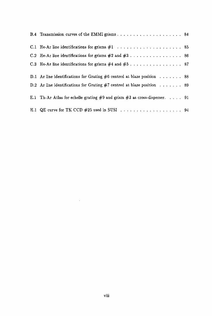
BA Transmission curves of the EMMI grisms. . . . . . . . . . . . . . . . . . .. 84
C.1 He-Ar line identifications for grisms #1 85
C.2 He-Ar line identifications for grisms #2 and #3 . 86
C.3 He-Ar line identifications for grisms #4 and #5 . 87
D.1 Ar line identifications for Grating #6 centred at blaze position 88
D.2 Ar line identifications for Grating #7 centred at blaze position 89
E.1 Th-Ar Atlas for echelle grating #9 and grism #3 as cross-disperser. 91
H.I QE curve for TK CCD #25 used in SUSI ............... 94
viii
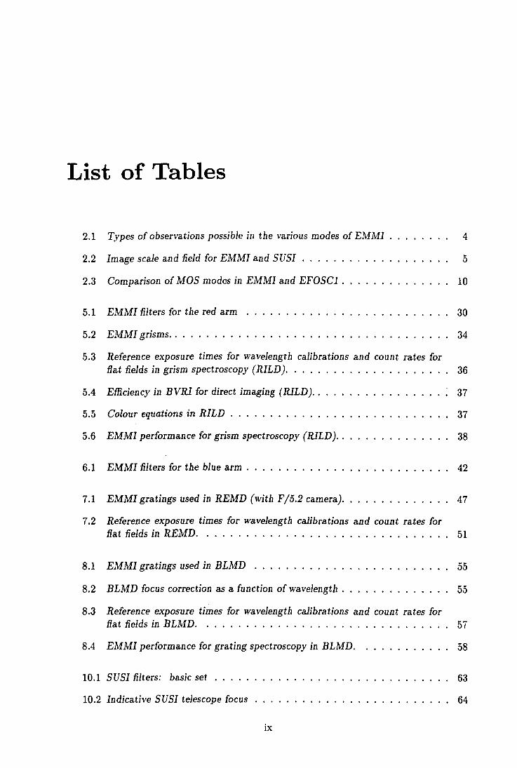
List of Tables
2.1 Types of observations possible in the various modes of EMMI .
2.2 Image scale and field for EMMI and SUSI ..... .
2.3 Comparison of MOS modes in EMMI and EFOSCl .
5.1 EMMI filters for the red arm
5.2 EMMI grisms. . . . . . . . . .
5.3 Reference exposure times for wavelength calibrations and count rates for
4
5
10
30
34
flat fields in grism spectroscopy (RILD). . . . . 36
5.4 Efficiency in BVRl for direct imaging (RILD) ..
5.5 Colour equations in RILD . . . . . . . . . . . .
37
37
5.6 EMMI performance for grism spectroscopy (RlLD). . 38
6.1 EMMI filters for the blue arm. . . . . . . . . . . . . . . . . . . . . . . . .. 42
7.1 EMMI gratings used in REMD (with F/5.2 camera) . ........... " 47
7.2 Reference exposure times for wavelength calibrations and count rates for flat fields in REMD. . ............................ " 51
8.1 EMMI gratings used in BLMD 55
8.2 BLMD focus correction as a function of wavelengtll . 55
8.3 Reference exposure times for wavelength calibrations and count rates for flat fields in BLMD. ............ . . . . . . . . 57
8.4 EMMI performance for grating spectroscopy in BLMD. 58
10.1 SUSI filters: basic set ..... 63
10.2 Indicative SUSI telescope focus 64
ix

11.1 Instrumental polarization of EMMI. . . . . . . . . . . . . . . . . . . . . .. 72
A.l Main window of EMOS. . . . . . . . . . . . . . . . . . . . . . . . . . . . .. 76
x

Chapter 1
Introduction
This manual describes the operation of the ESO Multi-Mode Instrument (EMMI) at the New Technology Telescope (NTT) on La Silla. This intermediate version was prepared after installation of the F /5.2 camera in the red arm in February 1994. It is an update and a complement of the previous version. Not all calibrations of this new camera have been performed yet. A final version will be issued by the end of 1994. Updated information can be obtained from the ESO Bulletin Board by telnet to mc3. hq. eso. org and using the login: esobb. Important changes or technical improvements are regularly described in The Messenger.
The NTT and EMMI can be operated in remote control from Garching. The user interface in Garching is different from the .one on La Silla mountain. That user interface is described in the Remote Control manual (ref [1]) available from the Visiting Astronomer Section in Garching.
EMMI is a very flexible instrument which allows a wide range of observing modes, from wide-field imaging to high-dispersion echelle spectroscopy, including long-slit and multiobject spectroscopy. This manual also includes SUSI (SUperb Seeing Imager) which, although m.ounted in' the other Nasmyth focus of the NTT, complements the capabilities of, and can be used concurrently with, EMMI. A brief description of the active optics system of the NTT and its basic operational principles are also provided in this manual.
The driving concepts in the instrument definition were the high image quality foreseen for the NTT, the need to complement or improve 3.6m instrumentation, and the need to minimize instrument change-overs. The concept which was adopted is that of a dual-beam instrument, fully dioptric, and based on the white pupil principle. CCD detectors were foreseen for the two arms with the possibility to adapt to the geometric characteristics of future detectors by changing the cameras only. The main advantages of this type of design are the high efficiency in both channels and the easy conversion from wide field imaging to grism and grating spectroscopy.
After the first observations with the NTT, it became clear that the telescope and the atmosphere at La Silla could provide stellar images with diameters as good as 0.3". Images of this quality could not be sampled adequately with EMMI, whose scale had also to be adapted to the spectroscopic modes of observation. Thus, SUSI was designed and built
1

2
for the other N asmyth arm of the NTT.
The structure of the manual is as follows.
Chapter 2 is an overview of the instrument which briefly summarizes what can be done in the various observing modes. It will be noticed that for most of the modes, EMMI is not a unique facility at La Silla. Low resolution spectroscopy with grisms for example can be done with EFOSC at the 3.6m telescope, grating spectroscopy with CASPEC also at the 3.6m. Experience gained with these instruments is directly useful for the corresponding modes of EMMI.
Chapter 3 describes the user interface of EMMI in general (Le. the interface with the instrument control software), that is: how to start? how to select a light path? how to define an exposure? focus the instrument for a given mode? etc. All functions of the instrument are fully computerized and remotely controlled once the setup has been made. That chapter also includes a check list for observations.
Chapter 4 gives a short overview of the active optics system of the NTT.
Each mode of the instrument is described in its own Chapter (5 to 9) which includes sections on selecting a setup, focussing, pointing, observing, calibrating data etc.
The imaging modes in the red and blue arms are of special relevance because they are used for focussing the telescope. Focussing with a focus wedge is explained in Sect. 5.3.1 and using a through-focus sequence in Sect. 6.3.1.
Observing with SUSI is described in Chapter 10.
More information on the optics (distortion, ghosts etc) can be found in Chapter 11.
The interface of the telescope control software, operated by the night assistant, provides parameters on the dome and telescope status (windscreen, mirrors, hydraulic system, etc), the positions of the telescope and the rotator(s), the guide probe(s), some external parameters ( e.g. wind speed) . This interface is not documented in this manual. Please ask your night assistant and introducing astronomer all questions you would like to know. The night assistants are also responsible for the operation of image analysis. They are acquainted with the judgement of the parameters. It is recommended, however, that observers participate in operational decisions that will affect their data. Basic information on that subject is provided in Appendix E .
Information on the current technical activity at the telescope and the problems encountered during the previous nights and weeks can be obtained by going through the NTT report facility. By typing nttrep on any workstation on La Silla, you will have access to technical problems concerning the various subsystems of the telescope ordered by type or by date. The interface is self explanatory.

Chapter 2
Instrument Overview
2.1 Optical design
A detailed description of the optical design of EMMI can be found in Dekker et al. (1986). Figure 2.1 shows the optical layout and identifies the main components of the instrument. The blue channel is coated for high efficiency in the region 300 to 500 nm, the red one for 400 to 1000 nm. There are various modes of operation in each channel, and efficiency curves for the various modes are given in Appendix B.
INlMCfaIe I I~I IWE CCD RED CCD c:...r ~
F=
ij~~~~~I~~~I~1m~~~~~~~~~ ~ 1=
F= 1=
.................. Glalingunil ~----------~ ~------------~ ILUE lED
Figure 2.1: Schematic layout of EMMI showing location8 of the main components.
3
4 CHAPTER 2. INSTRUMENT OVERVIEW
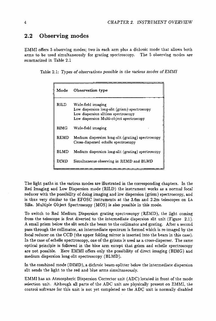
2.2 Observing modes
EMMI offers 5 observing modes; two in each arm plus a dichroic mode that allows both arms to be used simultaneously for grating spectroscopy. The 5 observing modes are summarized in Table 2.1
Table 2.1: Types of observations possible in the various modes of EMMI
Mode Observation type
RILD Wide-field imaging Low dispersion long-slit (grism) spectroscopy Low dispersion slitless spectroscopy Low dispersion Multi-object spectroscopy
BIMG Wide-field imaging
REMD Medium dispersion long-slit (grating) spectroscopy Cross-dispersed echelle spectroscopy
BLMD Medium dispersion long-slit (grating) spectroscopy
DIMD Simultaneous observing in REMD and BLMD
The light paths in the various modes are illustrated in the corresponding chapters. In the Red Imaging and Low Dispersion mode (RILD) the instrument works as a normal focal reducer with the possibility of doing imaging and low dispersion (grism) spectroscopy, and is thus very similar to the EFOSC instruments at the 3.6m and 2.2m telescopes on La Silla. Multiple Object Spectroscopy (MOS) is also possible in this mode.
To switch to Red Medium Dispersion grating spectroscopy (REMD), the light coming from the telescope is first diverted to the intermediate dispersion slit unit (Figure 2.1). A small prism below the slit sends the beam to the collimator and grating. After a second pass through the collimator, an intermediate spectrum is formed which is re-imaged by the focal reducer on the CCD (the upper folding mirror is inserted into the beam in this case). In the case of echelle spectroscopy, one of the grisms is used as a cross-disperser. The same optical principle is followed in the blue arm except that grism and echelle spectroscopy are not possible. Here EMMI offers only the possibility of direct imaging (BIMG) and medium dispersion long-slit spectroscopy (BLMD).
In the combined mode (DIMD), a dichroic beam-splitter below the intermediate dispersion slit sends the light to the red and blue arms simultaneously.
EMMI has an Atmospheric Dispersion Corrector unit (ADC) located in front of the mode selection unit. Although all parts of the ADC unit are physically present on EMMI, the control software for this unit is not yet completed so the ADC unit is normally disabled

2.3. CAMERAS AND DETECTORS 5
by the Operations staff during the observations.
2.3 Cameras and Detectors
EMMI works with two scientific CCD cameras, one at the red arm and one at blue arm. An intensified TV camera provides images of the central field of view of the telescope as reflected off the slit jaws in modes REMD, BLMD, and DIMD.
The image scale at the F/ll Nasmyth foci of the NTT is 5.36 arcsec/mm or 186 micron for 1 arcsec. This is also the scale of the direct imaging with SUS!. The actual field size and scale depend on the detector and camera being used and are given in Table 2.2.
Table 2.2: Image scale and field for EMMI and SUSI
Mode CCD type Camera Pixel size Field (JLffi/arcsec) (arcmin)
EMMI RILD TEK 2048 F/5.2 24/0.27 9.15 x 8.6
EMMI BIMG THX 1024 F/4 19/0.29 4.9 x 4.9 EMMI BIMG TEK 10241l F/4 24/0.37 6.2 x 6.2
SUSI TEK 1024 24/0.13 2.2 x 2.2
a. In use at present.
As these detectors may be changed on short notice, the details of their characteristics will not be all included in this manual, but can be found in the ESO CCD manual or by invoking the MIDAS context FILTERS (only under X windows) where the basic properties of CCDs available on La Silla are given. We give in the present manual information on the CCDs presently mounted on EMMI in Chapter 5 (RILD) for the red camera, Chapter 6 (BIMG) for the blue camera and Chapter 10 for SUS!. Updated information may be obtained from the ESO bulletin in Garching using: telnet me3. hq. eso. org, login: esobb. Technical problems encountered with the detectors ( e.q. pick up noise, bias gradient etc.) would be described in the NTT report facility which can be accessed by typing nttrep on any La Silla workstation.

6 CHAPTER 2. INSTRUMENT OVERVIEW
2.4 Instrument set-up
This section describes which options are available. How to operate the corresponding modes is described in Chapters 5 to 10.
For each mode of EMMI there are a number of elements that can be installed in order to , configure the instrument to your specifications. Thus, there is a range of filters, grisms,
slits, deckers, and gratings which can be mounted on the instrument. Not all of these components can be mounted together and therefore you must specify the instrumental configuration required for your observations. This has to be done one day before your observing run by filling out a special form available at the Astronomy Lounge on La Silla. The characteristics of the optical components of EMMI are given below.
Please note that ESO is not committed to make available instrument configurations which deviate significantly from the one requested with the original application.
2.4.1 Imaging in the red arm (RILD mode) and in the blue arm (BIMG mode)
EMMI has four filter wheels: the blue and red imaging filter wheels, and the blue and the red below-slit wheels. Usually these only hold neutral densities. Each of the two filter wheels used for imaging has 9 positions of which only 8 are available for mounting filters and one is always free.
All filters are permanently mounted in special cells which make replacement very easy. Although it is possible to use blue filters in the red and vice versa (one might want to do this in the overlap region, 400 to 500 nm), filters should normally be used in the wheel they are intended for. Red arm filters are mounted at 5° inclination to avoid reflections between the CCD and the filter. Blue arm filters, used in the converging beam in front of the blue camera, do not show this effect and are hence mounted with no inclination. The transmission curves of these filters are given in the ESO Image Quality Filters Catalogue (Gilliotte, 1992), and can also be obtained using the MIDAS context FILTERS.
EMMI red filters satisfy the requirement of image quality (as described in the ESO Image Quality Filters Catalogue) since they are operated in a parallel beam. Both red and blue filters have a free diameter of 80 mm and an outside diameter of 85 mm. Adapter trays are available for filters of other instruments (e.g. EFOSC) but use of smaller filters will produce vignetted images only useful in the centre of the CCD. The lists of standard EMMI filters are given in Chapters 5 (RILD) and 6 (BIMG) respectively (Tables 5.1 and 6.1). Some filters introduce a shift in the focus of EMMI. These focus offsets, measured in the instrument, are given in the tables whenever available. Offsets for other filters can be measured in RILD mode using the focus wedge with a pinhole mask in the aperture wheel, and the procedure FOCUS (Appendix A). In BIMG the focus offsets must be measured from stellar images.
2.4. INSTRUMENT SET-UP 7
-- GRISMS AND ECHEU!S I),). fiXED)
50.000 _-- GRATINGS ().~ ADJUSTABLE)
GRTIO SAl",,,,
20.000
/ , OO6281/mm / ..... /' ......
10.000 I' ...... , ... ;1' ..,. ... ... ..,.
GRT9IB1t",m I' ... > d
Rs GIn 1\ 6.11/"",,1' " ... ..,. ... ' .SOOO ... " GRT7 MA/mm ,,'" .---.-'" ;' ...... , ...
",4' ...... .,/ ,-...... ..,.' , ...
" ... ... ... GRTB all""" GRll 17.sl/mni ,,~ --,," --.... -... --2000 ;!"-- .,..,,-- . ",,'" ...... GRS6 102.1,6nm f" I > ....
," , ... ...... GRT 13 230l/rrm ", , ...
GRT \2 38l/mm .... ...' .............. GRS5 l12l~ d • --~~ ... -lOOO ~ .... _ ... _ .... R ......
.... ", ... ' 1' .... ,. .rC
,,'" GRT~ nlfmm '; <
500 ,," t$'"
~~ .... ", ,
GIn S tsolimm • GRS 1 515,ynm
200
3000 AOOO 6000 7000 1000 9000 1O.QOO
MA)
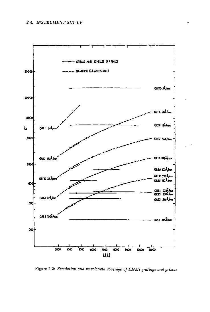
Figure 2.2: Resolution and wavelength coverage of EAlM! gmtings and grisms

8 CHAPTER 2. INSTRUMENT OVERVIEW
2.4.2 Long-slit spectroscopy in the red arm (RILD, REMD) and the blue arm (BLMD)
For spectroscopic observations, EMMI has a grism wheel in the red arm and two grating units, one in each arm. Each grating housing mounts two gratings back to back; in this way the user has a choice of 4 gratings in a given observing night. Seven housings, four for the red arm and three for the blue, are presently available. The allocation of gratings to a given housing is permanent. No change of grating is possible during the night. Figure 2.2 provides a global view of wavelength coverage and slit-resolution products (Rs, nominal resolving power for a 1 arcsec slit) of the grisms and the gratings. The characteristics are listed in more detail in the chapters corresponding to the various modes of the instrument. The efficiencies are given in Appendix B.
Low resolution spectroscopy with grisms (RILD mode)
Low resolution spectroscopy is usually done in the red arm using grisms (RILD mode). With the present F /5.2 camera and the TEK 2048 CCD the slit length is 8 arcmin. The widths of these slits (called starplates in the EMMI control software) are fixed. So in order to change slit widths a new starplate must be selected. The slit wheel has 5 positions, of which one is kept free for direct imaging. Thus, up to 4 long slits can be mounted at any given time. Available widths are 0.5",1.0",1.5",2.0",5.0", and 10".
The list of available grisms for the red arm is given in Chapter 5 (RILD). These are permanently mounted on special bayonets which make replacement very easy. However, changing during the night is not recommended due to the need of aligning the dispersion direction with the CCD pixels. Notice, however, that the grism wheel of EMMI has 9 positions out of which one is kept free for direct imaging, one is used for the focus wedge and two are reserved for cross-dispersion in echelle spectroscopy. Examples of He-Ar spectra obtained through the EMMI grisms are presented in Appendix C.
Slit less spectroscopy with narrow band filters (RILD mode)
In RILD mode grisms and filters can be combined to obtain slitless spectra imaged on the CCD camera. This mode of operation should be useful in a number of survey programs. The use of filters in combination with a grism reduces the sky background intensity. It also selects the wavelength region of interest and limits the length of the spectrum. The spectral coverage within this T~gion depends on the image position of the object.
Spectroscopy with gratings (REMD and BLMD modes)
Low and intermediate dispersion spectroscopy in both arms (modes BLMD and REMD) is possible using gratings. The REMD mode offers two echelle gratings for high dispersion work and the BLMD mode offers one high dispersion non-echelle grating. The length of the slit in the intermediate dispersion modes is 6 arcmin in BLMD and REMD, but the useful length is determined by the detector/camera combination. The slit width in these modes can be continuously adjusted between 0 and 9 arcseconds. The slit length
2.4. INSTRUMENT SET-UP 9
in the echelle mode must be limited using an adjustable decker to match the interorder separation.
The properties of the gratings available in the blue and red arms are listed in Chapters 7 (REMD) and 8 (BLMD).
Notice that, as is the case for some grisms, order separating filters are required for some of the gratings in mode REMD. These filters are mounted in the standard filter wheel and therefore affect the focus of the instrument for their offsets as tabulated in Table 5.1.
Echelle spectroscopy (REMD)
There are two echelle gratings (#9 and #10) which can be used in combination with a cross-dispersing grism to obtain data in an echelle format. The echelle grating #9 is mounted in a standard grating housing, but echelle grating #10 is mounted in a special unit. The installation requires using the crane in the instrument room and takes longer than for a standard grating. A movable decker is mounted to limit the length of the slit. The choice depends on the spectral region to be observed and on the grism used as cross-disperser. The relevant properties of the echelle spectra obtained using different cross-dispersers are described in Chapter 7 (REMD). A third echelle grating has recently been tested. It will be described in a future issue of the Messenger. The echelle gratings can also be used with narrow-band filters for high resolution long slit spectroscopy.
The dichroic mode (DIMD)
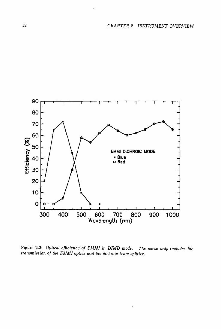
A dichroic beamsplitter can be inserted in the beam in mode DIMD to allow simultaneous medium to high dispersion spectroscopy with gratings in the red and blue arms. This beam splitter is permanently mounted in the instrument and cannot be exchanged. The efficiency curve of the presently available unit is shown in Figure 2.3. The central wavelength is approximately 450 nm.
2.4.3 Multislit spectroscopy (RILD)
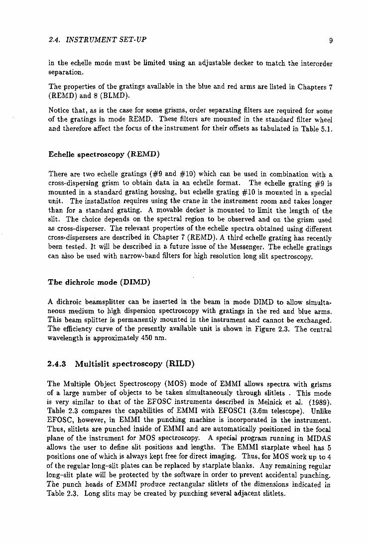
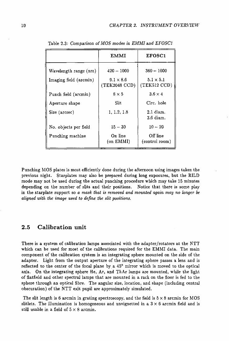
The Multiple Object Spectroscopy (MOS) mode of EMMI allows spectra with grisms of a large number of objects to be taken simultaneously through slitlets . This mode is very similar to that of the EFOSC instruments described in Melnick et al. (1989). Table 2.3 compares the capabilities of EMMI with EFOSCI (3.6m telescope). Unlike EFOSC, however, in EMMI the punching machine is incorporated in the instrument. Thus, slitlets are punched inside of EMMI and are automatically positioned in the focal plane of the instrument for MOS spectroscopy. A special program running in MIDAS allows the user to define slit positions and lengths. The EMMI starplate wheel has 5 positions one of which is always kept free for direct imaging. Thus, for MOS work up to 4 of the regular long-slit plates can be replaced by starplate blanks. Any remaining regular long-slit plate will be protected by the software in order to prevent accidental punching. The punch heads of EMMI produce rectangular slitlets of the dimensions indicated in Table 2.3. Long slits may be created by punching several adjacent slitlets.
10 CHAPTER 2. INSTRUMENT OVERVIEW
Table 2.3: Comparison of MOS modes in EMMI and EFOSCl
EMMI EFOSCl
Wavelength range (nm) 420 - 1000 360 - 1000
Imaging field (arcmin) 9.1 x 8.6 5.1 x 5.1 (TEK2048 CCD) (TEK512 CCD)
Punch field (arcmin) 8x5 3.6 x 4
Aperture shape Slit Circ. hole
Size (arcsec) 1, 1.2, 1.8 2.1 diam. 3.6 diam.
No. objects per field 15 - 30 10 - 20
Punching machine On line Off line (on EMMI) (control room)
Punching MaS plates is most efficiently done during the afternoon using images taken the previous night. Starplates may also be prepared during long exposures, but the RILD mode may not be used during the actual punching procedure which may take 15 minutes depending on the number of slits and their positions. Notice that there is some play in the starplate support so a mask that is removed and mounted again may no longer be aligned with the image used to define the slit positions.
2.5 Calibration unit
There is a system of calibration lamps associated with the adapter/rotators at the NTT which can be used for most of the calibrations required for the EMMI data. The main component of the calibration system is an integrating sphere mounted on the side of the adapter. Light from the output aperture of the integrating sphere passes a lens and is reflected to the center of the focal plane by.a 45° mirror which is moved to the optical axis. On the integrating sphere He, Ar, and ThAr lamps are mounted, while the light of flatfield and other spectral lamps that are mounted in a rack on the floor is fed to the sphere through an optical fibre. The angular size, location, and shape (including central obscuration) of the NTT exit pupil are approximately simulated.
The slit length is 6 arcmin in grating spectroscopy, and the field is 5 x 8 arcmin for MaS slitlets. The illumination is homogeneous and unvignetted in a 3 x 6 arcmin field and is still usable in a field of 5 x 8 arcmin.

2.6. FORMAT OF THE SCIENTIFIC DATA 11
2.6 Format of the scientific data
The data from the EMMI and SUSI detectors are simultaneously transmitted to the IHAP and the MIDAS databases. MIDAS runs on a Unix workstation equipped with a DAT tape unit. IHAP uses standard 1/2 inch 2400 foot tapes at 6250 BPI with a total capacity of 45 1024 x 1024 images in FITS format.
The FITS format is strictly according to the ESO policy to archive fully the EMMI data and make them later available to the general users. The FITS headers of CCD files contain all the information necessary for the scientific use of the data, that is all the telescope, instrument, and detector parameters have the time information. At present, archiving is done using the IHAP system. Thus, observers are requested to save their data using IHAP even if they use the DAT storage concurrently. Notice that the full header information is not stored in the IHAP header, but ill FITS keywords. Therefore, the soft key I LIST FITS KEYS I must be used instead of DLIST to display the information on the IHAP terminal. Only when the files are written to tape are data and header information merged. The user will receive at the end of his/her run a DAT on which the data from the IHAP 1/2 inch tapes have been copied.
The DAT tapes used by the observer at the workstation for prereduction are not archived, and it is the observer's responsibility to manage these tapes. 60 m DAT tapes can be obtained from the Astronomy Secretary on La Silla.
12 CHAPTER 2. INSTRUMENT OVERVIEW
90~~~--~~~-r~-'--~~~-r~-'~
80
70
60
20
10
O...o-~
EMMI DICHROIC MODE • Blue o Red
300 400 500 600 700 800 900 1 000 Wavelength (nm)
Figure 2.3: Optical efficiency of EMMI in DIMD mode. The curve only includes the transmission of the EMMloptics and the dichroic bwm splittfr.

Chapter 3
Observing with EMMI
3.1 Instrument control
The NTT is controlled by two HP1000/ A900 computers, one for the telescope (called NTT) and one for the instruments (called NTI). The control software of EMMI is organized in such a way that EMMI is presented as 5 sub-instruments called RILD, REMD, BIMG, BLMD, and DIMD. Depending on the type of observations, the user selects one of these modes and the control software automatically moves the functions to be set for this mode. This leaves only the parameters of the particular type of observation to be defined. For instance, when setting up an exposure in RILD, the required mirror unit and the upper red folding mirror are automatically set. The observer must only specify the camera focus, the setting of the slit, filter and grism wheels, and the CCD exposure parameters.
3.2 User interface
The user interface (UIF) consists of a RAMTEK monitor where mouse driven menus and forms are displayed, and a normal CRT (LU:53) where messages from the system are given and commands may be entered. Parameters are entered by filling forms in the RAMTEK screen. IHAP and MIDAS are available on-line, and data storage is simultaneously possible in both systems. IHAP is run 011 terminal LU:65 and MIDAS on the Unix workstation.
Once all optionnal optical elements are installed according to the observer's request, a set-up form is produced. A printout of this form is delivered to the observer to be used as reference during the night and to verify the setup. The configuration of each mode will be displayed on the RAMTEK UIF whenever a setup is defined. An example of a typical EMMI setup form is reproduced in Figure 3.1. .
13

14 CHAPTER 3. OBSERVING WITH EMMI
._._ ........ __ ... _ •• __ ........... _ ....... _____ .... K2 ___ =.=-...... __ =~ __ ... .
EKKI OPTICAL SETUP TEL: NTT OBS:_______________ SETUP By:________________ DATE: _________ _
ADC prisms: 0.5" ,1. 0 ' , ,1. 5 ' , , 2.0" , free
Blue imaging (BIMG) Red Imaging and Low Dispersion (RILD)
Blue filter wheel (FILB) Red filter wheel (FILR) Grism wheel (GRIS) focus
name identifier offset name identifier offs. name identifier 1 B #603 -3 1 z #611 3 1 #1 #1 ALIGNED 2 U #602 40 2 H alph #654 5 2 #2 #2 ALIGNED 3 OIl/5 #649 0 3 V #606 32 3 #3 #3 ALIGNED 4 HE II #588 0 4 R #608 0 4 #4 #4 ALIGNED 5 He I #587 0 5 I #610 3 5 #5 #5 6 FOCW+B #604 focwB 0 6 Bb #605 2 6 #6 #6 ALIGNED 7 #1 HARTMANN 0 7 HALPHA #596 11 7 CD FREE 8 #2 HARTMANN 0 8 BG 38 #543 0 8 FOCW ALIGNED 9 FREE FREE 0 9 FREE FREE 0 9 FREE FREE
Starplate wheel (STAP)
name identifier 1 FREE FREE 2 5' , X"555.75 3 1.5' , X=552.8 4 2.0 X-555.7 5 MOS REDOO0100
focus - 0.0 + 20.0 • T focus -7994.0 + 9.7 • T T in deg C --_ .................... ----........ _-----....................... --... --... . BLue Medium Dispersion (BLMD)
Blue grating unit (GRTB)
name identifier # 3 1200 g/mm # 5 158 g/mm
Below slit filter wheel blue (BSLB)
focus name identifier offset
1 FREE 0 2 nd 1.0 ND 663 0 3 nd 0.5 ND 662 0
focus - 7613.0 + 39.0 • T
Red Medium Dispersion (REMD)
Red grating unit (GRTR)
name identifier # 10 31.6 g/mm
Below slit filter wheel red (BSLR)
focus name identifier offset
1 FREE 0 2 nd 0.5 ND 661 0 3 nd 1.0 ND 664 0
focus -7785.0 + 27.5 • T T in deg C .. __ .............. ----.................................................... . Dichroic Medium Dispersion (DIMD)
Blue focus offset - -25.0 I Red focus offset - -250.0
Figure 3.1: Example of a typical printed setup form of EMMI. The form shows the optical elements that have been mounted on the instrument, and the temperature dependence of the instrument focus.

3.3. GETTING STARTED 15
Besides showing the list of components mounted on the instrument, the form gives the temperature dependence of the instrument focus, the positions of the starplate slits for the RILD mode, and the filter focus offsets. The optical elements are mounted and aligned with the CCD rows by the operations staff. Check that your selected grisms are labeled ALIGNED and call the NTT coordinator (paging 93-50) should this not be the case.
3.3 Getting started
The program that controls EMMI is called OBST (OBServing Task). To run OBST, logon at the EMMI terminal (LU:53) with RTE-A LOG ON : OBST (no password is required; simply hit return when prompted), and follow the instructions appearing on the screen. During the initialization process, a special form called Assembly will appeal' on the OBST screen. The form requests the name of the observer and the programme identification, and asks you to set the flags which enable/disable communication with the relevant nodes of the NTT and CCD controllers. For normal operation during the night, all connections to these nodes (EMMI, CCDR, CCDB, ADAPTB, TELNTT) should be enabled (Le. set to I TRUE I). If you have to start the system during the day, when the NTT is stopped, fbf always set the , TELNTT I flag to', FALSE I. On the second terminal (LU:65), you may run IHAP by logging in with the username
EMMIHAP. After login, press the first soft key in the terminal (f 1: I ~ll) to start IHAP. A number of soft keys will appear that allow you to manipulate IHAP in the standard way.
Once OBST is running, EMMI is operated using mouse driven menus on the RAMTEK User Interface (UIF). In ord~r to operate the UIF, simply slide the mouse to the selected commands (that appear in bars on the right hand side of the RAMTEK monitor), and click at the desired command using the middle button of the mouse. EMMI is presented as 5 sub-instruments, each of which can be configured and operated independently. Thus, the observer is confronted with 5 different menus, one for each mode of EMMI. Clicking these menus leads to more menus and forms to be filled that allow to setup the instrument and define exposures. Up to 6 instrument setups and 8 exposures may be predefined for each mode. Much of this can be done during daytime or during integrations so that mixing observing modes during the night is a relatively straightforward task. It should be notice however that more observing modes means more calibrations which may become untractable in daytime.
On-line data reduction is possible both using IHAP and MIDAS. Both systems are fully implemented and the data are simultaneously transmitted to both systems. MIDAS runs on a Unix workstation with two monitors, the normal one used for standard MIDAS window, and one for image display. An automatic MIDAS procedure displays the new frames on this monitor. Data saving is possible both via IHAP and MIDAS, but only the IHAP data are archived and given to the Visiting Astronomer at the end of the observing run.
16 CHAPTER 3. OBSERVING WITH EMMI
3.4 Selecting the light path
3.4.1 Selecting the mode
During observations, the instrument configuration is done in two steps. First, the EMMI mode must be selected. This is done in the I Top menu I of the user interface. (This is
. the menu that appears after startup). After clicking I Top menu 1 the five EMMI modes appear on the VIr menu bar. Click the desired option. For example, for DIMD, click I DIMD-Dichr. Med. D .1. All clickings are performed with the central button of the mouse.
3.4.2 Selecting the setup
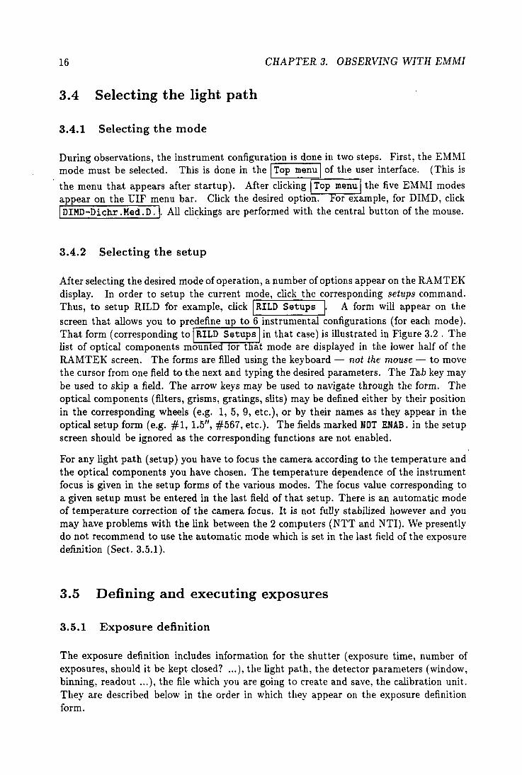
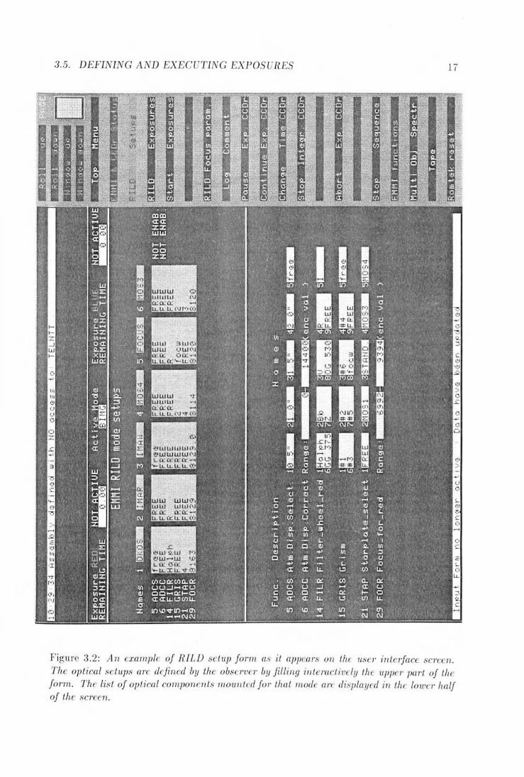
After selecting the desired mode of operation, a number of options appear on the RAMTEK display. In order to setup the current mode, click the corresponding setups command. Thus, to setup RILD for example, click 1 RILD Setups I. A form will appear on the screen that allows you to predefine up to 6 instrumental configurations (for each mode). That form (corresponding to RILD Setups in that case) is illustrated in Figure 3.2 . The list of optical components mounte or t at mode are displayed in the lower half of the RAMTEK screen. The forms are filled using the keyboard - not the mouse - to move the cursor from one field to the next and typing the desired parameters. The Tab key may be used to skip a field. The arrow keys may be used to navigate through the form. The optical components (filters, grisms, gratings, slits) may be defined either by their position in the corresponding wheels (e.g. 1,5,9, etc.), or by their names as they appear in the optical setup form (e.g. #1,1.5", #567, etc.). The fields marked NOT ENAB. in the setup screen should be ignored as the corresponding functions are not enabled.
For any light path (setup) you have to focus the camera according to the temperature and the optical components you have chosen. The temperature dependence of the instrument focus is given in the setup forms of the various modes. The focus value corresponding to a given setup must be entered in the last field of that setup. There is an automatic mode of temperature correction of the camera focus. It is not fully stabilized however and you may have problems with the link between the 2 computers (NTT and NTI). We presently do not recommend to use the automatic mode which is set in the last field of the exposure definition (Sect. 3.5.1).
3.5 Defining and executing exposures
3.5.1 Exposure definition
The exposure definition includes information for the shutter (exposure time, number of exposures, should it be kept closed? ... ), the light path, the detector parameters (window, binning, readout ... ), the file which you are going to create and save, the calibration unit. They are described below in the order in which they appear on the exposure definition form.
3.5. DEFINING AND EXECUTING EXPOSURES 17
Figure 3.2: An example of RILD setup form (IS it appears on I,he uscr' inte1face screen. The optical sel.llfJS m'e lle/ined by the ooser'veT' by filling illlcmc/itlcly fh e lIppe,- p(lrt of th e form. The list. of opticaL components f1lO1l11led for thai, m()(le are (/isplayed in lite Iowa /ullJ of the screen.
18 CHAPTER 3. OBSERVING WITH EMMI
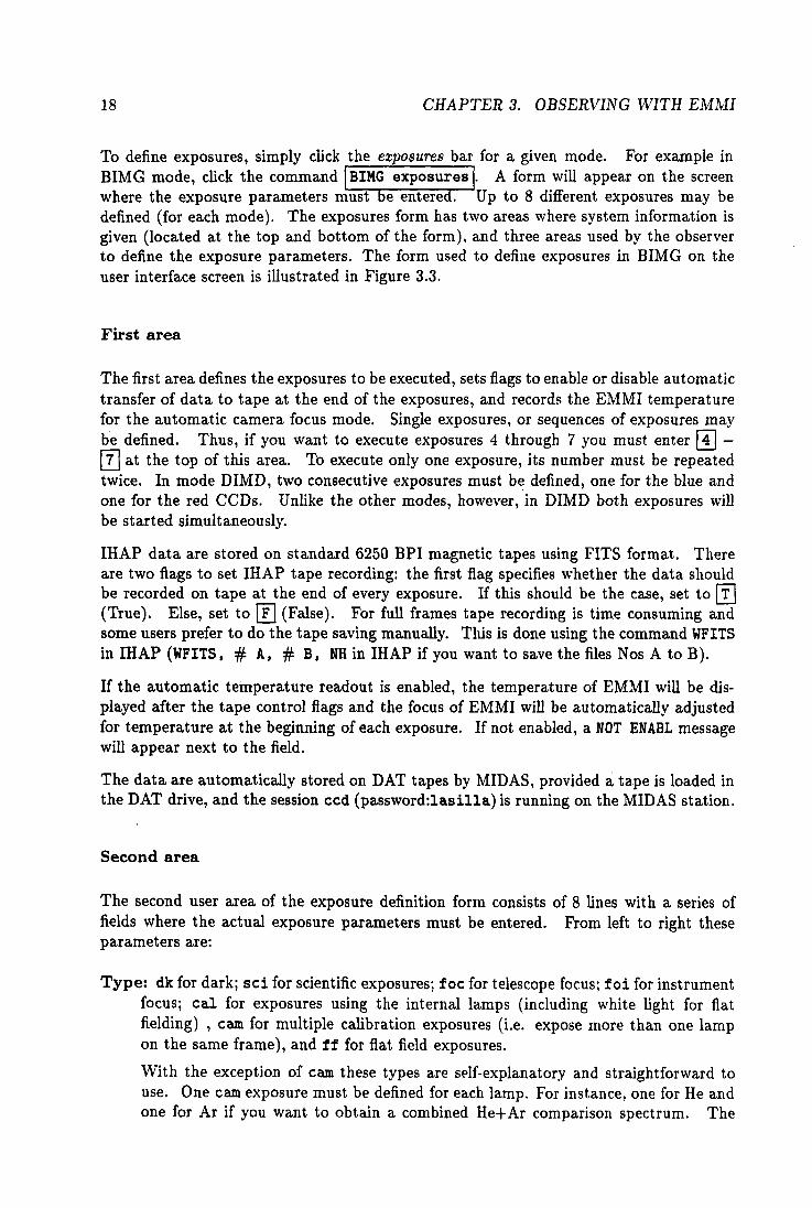
To define exposures, simply click the exposures bar for a given mode. For example in BIMG mode, click the command BIMG exposures. A form will appear on the screen where the exposure parameters must e entere. Up to 8 different exposures may be defined (for each mode). The exposures form has two areas where system information is given (located at the top and bottom of the form), and three areas used by the observer to define the exposure parameters. The form used to define exposures in BIMG on the user interface screen is illustrated in Figure 3.3.
First area
The first area defines the exposures to be executed, sets flags to enable or disable automatic transfer of data to tape at the end of the exposures, and records the EMMI temperature for the automatic camera focus mode. Single exposures, or sequences of exposures may bee defined. Thus, if you want to execute exposures 4 through 7 you must enter [II -[fJ at the top of this area. To execute only one exposure, its number must be repeated twice. In mode DIMD, two consecutive exposures must be defined, one for the blue and one for the red CCDs. Unlike the other modes, however, in DIMD both exposures will be started simultaneously.
IHAP data are stored on standard 6250 BPI magnetic tapes using FITS format. There are two flags to set IHAP tape recording: the first flag specifies whether the data should be recorded on tape at the end of every exposure. If this should be the case, set to [!] (True). Else, set to [!] (False). For full frames tape recording is time consuming and some users prefer to do the tape saving manually. This is done using the command WFITS in IHAP (WFITS, # A, # B, NH in IHAP if you want to save the files Nos A to B).
If the automatic temperature readout is enabled, the temperature of EMMI will be displayed after the tape control flags and the focus of EMMI will be automatically adjusted for temperature at the beginning of each exposure. If not enabled, a NOT ENABL message will appear next to the field.
The data are automatically stored on DAT tapes by MIDAS, provided a tape is loaded in the DAT drive, and the session ccd (password:lasilla) is running on the MIDAS station.
Second area
The second user area of the exposure definition form consists of 8 lines with a series of fields where the actual exposure parameters must be entered. From left to right these parameters are:
Type: dk for dark; sci for scientific exposures; foc for telescope focus; foi for instrument focus; cal for exposures using the internal lamps (including white light for flat fielding) , cam for multiple calibration exposures (Le. expose more than one lamp on the same frame), and ff for flat field exposures.
With the exception of cam these types are sE-If-explanatory and straightforward to use. One cam exposure must be defined for each lamp. For instance, one for He and one for Ar if you want to obtain a combined He+Ar comparison spectrum. The

" ~.
<l w w
~
"" o
'§' ~
;; 2. c = -if ;; o , ;:;" -• .;, g • o
~ = c "-.g, = •
i ;< • 5·
'" -0:
'"
,., " tl t'1 ." :;: :;: '" ,. '" '" '" ~ '" '" c:: ::l '" Cl l"'J
'" ." o <n
'" '" r-:; '"

20 CHAPTER. 3. OBSER.VING WITH EMMI
parameters in any set of cam exposures must be identical with the exception of the exposure time and the lamp number (or name).
Time: the exposure time in seconds must be entered in this field.
#n: this is the number of times a given exposure is to be repeated.
IHAP identifier: The exposure identification goes in this field. This identifier will be copied in the file header. The identifiers in any set of type cam exposures must be identical.
IHAP batch: enter here the name of an IHAP batch to be executed at the end of the exposure. The batch KDISPC may be used to display the image on the IHAP Ramtek. This is automatically done in MIDAS. If you do not intend to work with IHAP you may wish to enter CLEANIHAP. Then part of the IHAP database is deleted every time after a new exposure has been saved on tape, keeping only the 6 most recent files. In this way, a full IHAP database cannot temporarily block the observations.
Setup: in this field the number or the name of the instrument setup table must be entered (Sect. 3.4.2). The previously defined instrument setup tables appear in the lower half of the screen, so you don't have to remember or write down what you specified in each of the 6 possible setups for each mode.
Calib. lamp: enter in this field the name or the number of the calibration lamp you wish to use. The list of available lamps is displayed in the TCS Ramtek. Only one lamp should be specified.
In mode DIMD, an extra field Path appears in the exposure definition form that should be set to B or R according to which exposure is to be executed in the Blue or Red arm.
Third area
The third user area of the exposure definition form is used to set the CCD readout parameters. Binnin~x, y defines the number of pixels that will be combined in each direction. The default is w,[Ij where all the pixels of the CCD are readout independently. The next parameter that must be specified is the readout mode. Set the flag in the Fast readout mode field to [f] or []. In fast readout (T) the readout noise will be significantly larger, but the readout time will be cut by approximately 40%. The conversion factor between ADUs and electrons depends on the readout speed. For slow readout, this factor is significantly lower than for fast readout. Note that with the higher gain factor in fast readout, non-linearity and saturation are reached at correspondingly lower ADU values.
The exact values are periodically measured by the operations staff and are available in the EMMI control room. A marked noise pickup pattern may be present in bias frames taken in the fast mode. For these reasons fast readout is only recommended for tests and spectral calibrations. Also remember that, in general, calibration frames such as bias, fiat fields, and darks taken with slow readout cannot be used for correcting fast exposures, and vice versa.

3.5. DEFINING AND EXECUTING EXPOSURES 21
The W'indoW' readout field specifies the geometry of the CeD. If set to [!] the values that appear in the XL. XR (Left and Right borders), and YD. YU (Down and Up borders) fields are ignored and the full CCD is read out, including the over-clocked columns and rows. The full size of the frame including the over clocked pixels is given between parentheses. Note that IRAP can store and handle frames of at most 2048 x 2047 pixels (in any combination not exceeding the value of this product).
Note: Remember that if you window the CCD you may loose the overclocked pixels and thus the
possibility of checking the actual bias level of your science frames.
The CCD parameters apply to all exposures defined in the form and should therefore be changed before executing an exposure if you wish to use different values for different exposures (e.g. for direct imaging and spectroscopy). In mode DIMD two CCD readout forms appear, one for the red and one for the blue CCDs.
The last field of the form allows to enable the automatic temperature correction of the instrument focus. If set to [f] the EMMI camera focus will be automatically set to the value corresponding to the temperature displayed at the top of the form, taking the filter offsets into account. We presently do not recommend to use this feature which is not fully stabilized and suggest to set it to [!]. If set to [!], the focus value of the instrument corresponding to a given setup has to be entered in the last field of each setup (Sect. 3.4.2).
3.5.2 Executing exposures
To execute an exposure click the Start exposures command. This will not be possible if you are still in the exposure de mtlOn orm. n t at case, an error message will appear at the bottom of the Ramtek screen with ,an audible signal indicating that the mouse is disabled. Exit the form by pressing RETURN or ENTER in the keyboard. Wait for a series of beeps and a status message at the bottom of the screen: Input form no longer acti ve. Then you may start the exposure. The status of the instrument and CCD will" appear on the Ramtek screen. Warning: it is not immediately updated, this is done only when the exposure actually starts. After the instrument is configured, exposure status and integration time information will appear at the upper corners of the screen (upper left for the red CCDi upper right for the blue). This information will appear in every menu so you may safely change forms during exposures and still have information of the remaining time and instrument status. There are several bars in the UIF that allow to pause or abort an exposure, and change the exposure time. In order to prevent accidental execution of these commands, OBST prompts for confirmation. The command 1 EMMI i: CCO status 1 provides at any time full information about the status of EMMI and the CCDs. In DIMD, there are separate forms for EMMI (I EMMI status I) and for the CCDs (I CCOr i: CCDb status I).
Note: Exposure and setup definition of an ongoing exposure cannot be changed, except for the
exposure time.

22 CHAPTER 3. OBSERVING WITH EMMI
3.6 Check list
1. Have a look at the notice board in the control room. You will get a first view on the technical activities or changes at the telescope. Should you wish to know about the problems encountered with the instruments, detectors, adapters, telescope ... in the previous days or weeks, type nttrep on the workstation and follow the instructions. The NTT report facility is self explanatory.
2. To inform yourself about day-time work at the NTT type nttcal which will display a mouse-driven calendar.
3. Compare the optical setup form with your request.
4. When starting OBST on EMMI terminal (LU: 53) check the connections to the nodes (EMMI, CCDR, CCDB, ADAPTB, TELNTT). During day time TELNTT must be set to FALSE.
5. If you are not familiar with the user interface, prepare as an exercise for example a calibration exposure of 1 sec with a grism, a He lamp that will be read in fast readout and start the exposure. It takes some time to send the information from the interface to the instrument. It takes additional time to rotate the wheels, move the mirrors, heat the lamps etc. Thus after you fill a form, press RETURN and wait for the audible signal before using again the keyboard or the mouse.
6. Check the readout noise of the detector( s) on bias exposures. Check for any gradient in the bias.
7. By running exposures with various setups, you may find that one of the functions cannot be initialized (a message appears on EMMI terminal LU: 53). Call the NTT coordinator using 93-50 (paging system).
8. In the afternoon the alignment of the slits with the CCD can be checked by using calibration exposures.
9. It is very advisable to begin the preparation of MOS tables as early as possible.
10. The first exposures of the night, including focus exposure and quick look exposure of the field, may be defined in advance.
11. After starting an exposure, check the instrument status display. Make sure that the correct slit, filter or order sorting filter, grism or grating, cross-disperser grism and echelle etc. are switched in.
12. Check the CCD readout mode and binning.
13. Did the exposure (count down of exposure time) actually start?
14. After starting an exposure, look for any error message on the EMMI terminal (LU: 53). Check the monitor regularly because messages may scroll off the page and, therefore, escape notice. Messages are confined to the upper half of the screen. Always check the time for the most recent message.
15. Check EMMI, dome and CCD temperatures from time to time.

3.7. THE NTT REPORT FACILITY 23
16. Check the seeing and focus regularly. The seeing measured by the seeing monitor can be obtained in the Meteo plane on the workstation (Sect. 4.4) by typing x (without RETURN) in the meteomonitor window.
17. Is the target on the slit?
18. Is the telescope guiding?
19. Is the remaining rotator angle range sufficient for your long exposure?
20. Do not forget to consider seeing effects when estimating exposure times for narrow slit observations.
21. Check the parallactic angle of the slit.
22. Is the central wavelength of the grating correctly set?
23. Are the slit width and heigth adequate to the required resolution, leaving enough inter-order space?
24. If the seeing becomes excellent « 0.7"), always make an image analysis close to the observing field.
3.7 The NTT report facility
A computer based system has been installed for reporting technical problems encountered by the astronomers using the NTT, and follow-up by maintenance staff. This NTT report facility is used as a source for tracking anomalies, actions which have been taken, solutions, receipes for future problems and NTT upgrading. It replaces the printed night reports . The observers have access to the reporting system by typing nttre.p on the workstation. A window interface appears that is self explanatory. Astronomers can read previous reports on the telescope and instruments, and submit reports as they used to do with the night reports on paper.
3.8 The NTT daytime activities calendar
3.9 Troubleshooting
Error and status messages are printed at the top and the bottom of the Ramtek UIF, and on the OBST console.
A reserved area at the very top of the UIF gives error messages that need to be specifically cleared. For example, if OBST is assembled with the link to the NTT computer disabled, a message reading: Assembly defined with NO access to: TELNTT will appear in yellow, preceded WIt t Ie tIme at w IC t IS partIcu ar con This does not imply necessarily a catastrophic failure.

24 CHAPTER 3. OBSERVING WITH EMMI
The messages at the bottom of the UIF inform you whether the system expects input from the mouse or from the keyboard, and whether the parameters in the forms have been sent to the computer. Normally these conditions are cleared by simply sending the forms (using the RETURN or ENTER keys) before using the mouse. Sometimes, however, the terminal stays inactive and does not acknowledge input from either the keyboard or the mouse. In that case, hit RETURN several times until the condition is cleared. If the terminal continues to be blocked, go to another terminal of the NTI computer (not NTT) and from CI type CI> SETP ,lu where lu is the logical unit of the terminal you wish to unblock (usually written on the terminal itself). If this does not work, ask your night assistant for help, and eventually call Operations (paging system 93-34 during the night).
The third list of messages appears on the upper half of the OBST console. These messages contain information about the current activity of the system, as well as error messages. They are normally not ordered so you must check the time that is displayed together with the message to find the most recent ones. The error messages usually inform of some failure that prevents an exposure from being started (for example if a wrong parameter is given in one of the forms or if there is an ongoing exposure).
A common error message occurs when the IHAP database is full. The message I IHAP database full I appears before the exposure starts. In that case, the IHAP commands PURGE and PACK must be used to remove files and clear the disk space. Make sure that the files have been written to tape before using the PACK command. Files accidentally purged may be recovered using the FRESTORE command, but this is no longer possible once PACK is used.
Sometimes the frames arrive at the MIDAS workstation without the full list of descriptors (headers). This is due to a bug in the HP computers where a program called AOIB stops. This happens randomly and it is therefore recommended to check every afternoon if all the descriptors are present (use the MIDAS command READ/DESC filename * ). If only a short list of descriptors is present, ask the night assistant to restart AOIB.
The receipt of new exposures by MIDAS is reported in a window of the Unix workstation.
Chapter 4
Image analysis and Focus
4.1 Image analysis
Both primary and secondary mirrors of the NTT are actively supported. The active support of the primary (Ml) unit consists of 75 actuators and three fixed point supports. The M2 support provides X,Y,Z motions. The force applied to each of the 75 actuators can be adjusted and thus the shape of primary mirror can be modified. The X,Y motion of M2 is used to correct for decentering coma. Motions in Z allow to adjust the telescope focus.
The image analysis sytem, located inside the instrument adapter/rotators consist of a Shack-Hartmann grid and a CCD which are used to record images of the telescope pupil through the grid. Then a software loaded in the dedicated VME, processes these images, determines the corresponding telescope aberrations, and computes the differential forces to be applied to the active supports in order to correct these aberrations (Wilson et al. 1991 ).
The night assistants are acquainted with the system and are responsible for its operation. It is useful, however, that observers be aware of the basic operational principles since they may be requested to take operational decisions in nights of excellent seeing.
The NTT Active Optics System (AOS) is initialized every afternoon by the night assistant. In practice, this means setting the forces of the MI support, and the position of the M2 unit to the default values which have been calibrated for zenith position. Normally, this procedure alone is sufficient to operate the telescope under average seeing conditions (FW H M '" I"). In order to optimize the mirrors setting, the night assistants are instructed to do an image analysis shortly after sunset. The observers may decide to shift these measurements to later in the night if they conflict with the acquisition of twilight sky flat fields, but in general it is advisable to monitor the mirror settings at least once per night. A record of all active optics measurements is kept in the NTT control room.
For seeing conditions around one arcsecond there is no need to further check the AOS unless the images become distorted. The active optics system automatically corrects the position of the M2 unit as a function of zenith distance (in order to minimize coma).
25

26 CHAPTER 4. IMAGE ANALYSIS AND FOCUS
If the seeing conditions become exceptional (e.g. 0.5" or better), or if the conditions are good (e.g. < I") and the telescope is pointed to zenith distances larger than 30 0
, it is recommended to do an image analysis using a bright star near the position of every target field. An image analysis plus correction takes about 10 minutes, but soon it will be possible to do the image analysis during target acquisition. The correction will still be "done out of acquisition (cf. Appendix E).
4.2 Focusing the telescope
In the red arm, the focus of the telescope can be determined either using a throughfocus exposure sequence, or using a focus wedge similar to EFOSC. Only through-focus sequences can be used in the BIMG mode. The temperature dependence of the NTT focus is
~F / A T = 0.0764 mm;oC
The zenith distance correction is negligible if the active optics system for the main mirror is not in use. Otherwise, it is recommended to check the focus every time the optics are corrected (cf. Appendix F). The telescope focus is the same for the modes RILD, REMD, BLMD if no filters are used under the slit, so the focus wedge can be used for all EMMI configurations except BIMG, for which through focus sequences are in principle required for each filter. However, with the B filter in the blue arm, the BIMG focus and the RILD focus (no filter or R filter) are the same. The dichroic beam splitter used in D IMD introduces a focus offset in both arms. The values of these offsets are given at the bottom of the instrument setup form (cf. Figure 3.1).
Focussing with the focus wedge has to be done in the RILD mode, so this method is described in the Chapter 5 (RILD) . This is the fastest method for focussing. Focussing the blue arm of EMMI in BIMG can be done by using a through-focus sequence. The method is described in Chapter 6 (BIMG), but is also applicable to mode RILD.
4.3 Focusing the EMMI cameras
The focus of the instrument is normally checked by the operations staff. The optical set-up form gives the value of the instrument focus for the various modes and their temperature dependence. In the BLMD mode the temperature is critical and should be closely monitored.
As the temperature of the EMMI room is kept approximately constant by the air conditioning system, adjustments to the instrument focus should not be required during the night except for mode BLMD. The EMMI temperature as well as the telescope tube and mirror temperatures are displayed by the Telescope Control System (TCS) UIF screen ( a RAMTEK monitor located next to the EMMI display).
The focus of any mode can be changed manually from the instrument console using the commands EMMI >FOCB. value and EMMI>FOCR. value for the Blue and Red arms respectively.

4.4. THE SEEING FROM THE SEEING MONITOR 27
The instrument focus must be entered in the last field of each of the 6 instrument setup tables. These values will be applied at the beginning of each exposure. The temperature equations are also stored in the system. Thus, if the automatic mode is selected, the program checks the EMMI temperature, calculates the focus, and applies the filter offset. This, however, is done by the program only at the beginning of, but not during, an exposure. The EMMI focus is usually determined by the operation staff, but should you want to check the EMMI focus in a given mode, the procedures described in Appendix ~ can be followed.
4.4 The seeing from the seeing moni~or
Measurements from the seeing monitor can be obtained at any time by typing meteomoni tor on the workstation. A window appears on which you can type h (without RETURN) for help on the commands, x to create a new window in which the temperature, humidity, wind speed and seeing measurements of the last 24 hours period are displayed. meteomoni tor is started automatically in the Meteo plane of the workstation when the ccd session is started. To start the graphical representation of the met eo data, click on Meteo, then type x in the meteomonitor window.
Chapter 5
Observing in RILD
5.1 Optical configuration
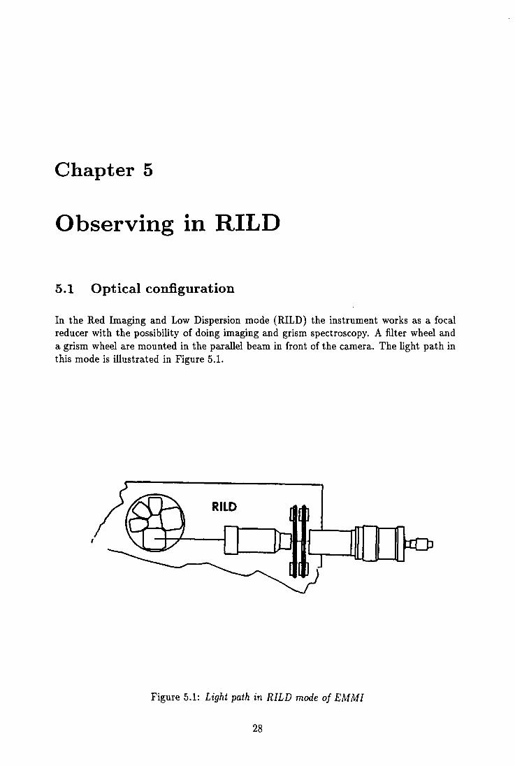
In the Red Imaging and Low Dispersion mode (RILD) the instrument works as a focal reducer with the possibility of doing imaging and grism spectroscopy. A filter wheel and a grism wheel are mounted in the parallel beam in front of the camera. The light path in this mode is illustrated in Figure 5.1.
RILD
Figure 5.1: Light path in RILD mode of EMMI
28
5.2. INSTRUMENT SETUP 29
5.2 Instrument setup
The instrument setup is done by selecting one position for each of the optical elements on the aperture (slit), filter, and grism wheels. This is done in the user interface by going first to 1 Top menu 1 then chosing the RILD mode by clicking ~. After selecting the mode
the setup can be done by clicking the setup command 1 RILD Setups I. A form appears on the screen that allows you to predefine instrumental configurations.
5.2.1 Slits
The aperture wheel has 5 positions, of which one is reserved for direct imaging. Thus up to 4 slits can be mounted at any given time. The widths of the currently available slits are 0.5", 1.0", 1.5", 2.0" , 5.0" and 10". After rotation of the wheel, a slit selected in RILD is oriented North-South.
5.2.2 Filters
Up to 8 filters can be mounted in the filter wheel. A list of the standard EMMI red filters available is given in Table 5.1. They satisfy the requirement of image quality since they are operated in parallel beam. Red arm filters are mounted at 5° inclination to avoid reflections. The transmission curves can be obtained by using the MIDAS context FILTERS. Observers who wish to use other filters are reminded of the image quality requirements. B photometry should normally be done in the blue arm of EMMI (Sect. 6.2.1). Image anomalies are described in Chapter 11.
5.2.3 {;risnas
The grism wheel has 9 positions, up to 5 of which are available for low resolution spectroscopy with grisms. One position is kept free for direct imaging, one position is taken up by the focus wedge, and two are used to mount the grisms for cross-dispersed echelle spectroscopy. The list of presently available grisms is given in Table 5.2. Five of them may be mounted simultaneously for RILD observations. They must be oriented such that the dispersion direction is aligned with the grid of CCD pixels.
More information on image quality, scale, distortion, ghosts, filter properties can be found in Chapter 11: Additional Information about EMMI.
5.2.4 Focussing the canaera
The optical setup gives a temperature dependant formula for the camera focus (in RILD) . Calculate the focus from this formula, add filter offset and enter this value in the last field of the instrument setup. In order to avoid an image degradation, it is recommended to refocus the instrument in mode RILD after a temperature change of'" 4°C in the EMMI room.

30 CHAPTER .5. OBSERVING IN RILD
Table 5.1: EMMI filters for the red arm
ESO Filter >'o/A>. (run) Peak efficiency Cell type Focus offsets (FWHM) % (encoder steps)
587 He I 448.0/5.0 55 R -22
588 He II 469.2 6.6 72 B 154 589 o III a 501.4 5.6 64 R 56 590 o III 3000 505.7 6.4 52 R +1 591 o III 6000 511.2 6.1 69 R 94
592 o III 9000 516.0 6.3 68 R +45 593 o III /12000 521.1 6.7 66 R 50 594 o III /15000 526.0 6.6 65 R 50 595 N II / 0 660.9/7.3 57 R 83 596 H Alpha / a 657.0/7.2 52 R +49 597 H Alpha / 3000 663.4/6.5 63 R +52 598 H Alpha 6000 669.4 6.8 57 R +16 599 H Alpha 9000 676.3 6.9 53 R +60 600 H Alpha 12000 683.4 7.2 61 R +82 601 H Alpha 15000 689.6 7.2 62 R 75 605 Bb 415[110 67 R -88 606 V 542/100 84 R +118 608 R 645/155 79 R 0 610 I 800/158 94 R 8 611 Z cut on 842 85 R -36 643 BG382rnm 480/320 97 R 9 644 GG3753rnm cut on 370 98 B -24 645 OG530 3rnm cut on 530 98 B 9 646 RG7153rnm cut on 722 98 R -7 652 He II 469.6 7.3 61 R 33 653 N II / 0 659.0 3.1 57 R +6 654 H Alpha 656.2 3.1 40 R +41 655 S II / 0 673.2 7.2 60 R +52 656 9150 913. 'U 19.4 92 R +95 657 sIll/a 953.2/10.0 93 R +64
5.2.5 Preparing exposure
By pressing I RILD exposures I you get the exposure form. Remember to specify the type of exposure (dk, sci, foc. cal, ff. cam), the setup previously defined, to choose or switch off the calibration lamps, check the binning, the readout mode and the window of the detector, transfer or not to tape.
5.3 0 bserving
5.3.1 Focussing with the focus wedge
Focussing in RILD can be done either with a fOCllS wedge or by using a through-focus exposure. We describe here the focussing with a focus wedge. The telescope focus is the same for the modes RILD, REMD, BLMD if no filters are used. Through-focus sequences

5.3. OBSERVING 31
are described in Chapter 6: Observing in BIMG, but they can be used also in RILD by clicking I RILD Focus param.' and following the same procedure as in BIMG.
To focus with the focus wedge you have to prepare a setup in RILD where the light goes through a focus wedge and possibly through a filter. Thus click 1 RILD I, then RILD Setups and in that form prepare a setup including the focus wedge and possibly a ter. ocus the camera according to the temperature. When this is ready prepare an exposure by clicking the command I RILD exposures ,. In order to average out seeing effects, do not
use excessively short exposures « 20sec) for focussing.
The focus wedge divides the pupil into two halves and separates the two images horizontally by a fixed amount. The vertical separation between the centroids of the two images depends on the defocusing and has been calibrated empirically. For a fair range of focus this dependence is linear, but gets rather complicated if defocusing is severe. To use the focus wedge proceed as follows: take a short exposure image using the focus wedge in the grism wheel and a filter (to minimize atmospheric dispersion). The use of fast readout and windowing is recommended to reduce the overheads. You will see two images for every object in the field. Use the batch FOCUS (MIDAS). This program, described in detail in Appendix A, gives the focus offset to be applied to the telescope. For the reason described above, if the focus offset is large (say more than 0.10mm) it is recommended to repeat the procedure. Normally, two exposures suffice to determine the focus to better than 0.010 mm, which is the accuracy required under good seeing conditions. The focus wedge works in a parallel beam and, therefore in principle, the focus is the same for all optical elements in the beam. In practice, however, some filters have optical power and therefore introduce focus offsets. The focus wedge is calibrated with no filter in the beam. Offsets introduced by the filters are listed together with the lists of available EMMI filters (Table 5.1).
Offsets for other filters can be measured (in RILD only) using the focus wedge with a pinhole mask in the aperture wheel. The batch FOCUS give the values to be applied to the instrument in encoder units. The focus wedge should be calibrated and this is normally done by the operations staff using the Hartmann masks. A quick check may be obtained taking an exposure of the pinhole mask mounted in the slit wheel and illuminated by the He or Ar lamps.
The surface of CCD # 36 is convex with a depth of 200 J.lm (between the edges and center). If the focus is done at intermediate focal position (500 pixels around the CCD center) the defocus blurr is less than one pixel, except for the extreme corners of the field.
5.3.2 Pointing and guiding
The pointing of the NTT is better than 2 arcsec rms. Therefore there is no need of checking the field before starting a RILD exposure in direct imaging.
Guiding the telescope during an exposure is usually done setting on a star with one of the two guide probes in the adapter and using the autoguider. This operation is normally carried out by the night assistant.

32 CHAPTER 5. OBSERVING IN RILD
5.3.3 Checking the seeing
The seeing can be checked on images taken in RILD by clicking the field I seein~1 that appears on top of the MIDAS display window. Move the cursor to an unsaturate star, click the left button of the mouse, repeat on several stars, stop the procedure by clicking the center button of the mouse. The size of the box may be adjusted with the arrow keys. The MIDAS procedure calculates the mean FWHM in X and Y directions. The seeing measured outside of the telescope by the seeing monitor can be displayed on the workstation by clicking Meteo or typing meteomonitor. A window appears which is self explanatory. Typing x in that window will create a new display with a graphical representation of the temperature, humidity, wind speed and seeing measured over the last 24 hours.
5.3.4 Direct imaging
The camera on the red arm of EMMI is at F /5.2 and the detector in use is a thinned TEK CCD of 20482 , 24J.Lm format. The scale has been found to be 0.268 ± 0.004 arcsec/pixel from measurements in an astrometric field. The unvigneted field of view is 9.15 x 8.6 arcmin corresponding to a format of 1 - 2086 (including overscan pixels) and 80 - 2020. The orientation of the images on the workstation screen is North at the top and East at the left.
The variation of the PSF across the field is approximately 5 % at the two perpendicular central directions x = 1000 and y = 1020. Variations up to 15 % occur in the corners of the field.
The time delay from the start of the read-out of one CCD image to its display on the workstation is relatively long. The delays in the one output mode for a full frame are 330s in slow mode and 225s in fast readout mode. If the transfer to the workstation is disabled the interval is 45s shorter.
The CCD can be read in dual ouput readout mode: two output preamplifiers are connected to the CCD, the upper half of the chip is read through one of the amplifiers, th~ lower half through the other. The gain is about 80s for the slow mode and 25s for the fast read-out mode.
For a quick look display of the full frame at reasonable resolution, use the dual output mode, 2x2 binning and a window of 1-2086 by 80-1967 pixels. The frame will be read and displayed on the WS in about 1 minute. Note however that the "binned" display of MIDAS is based on pixel skipping rather than re-sampling, so very fine details may get lost whereas any regular pattern may appear strongly amplified.
An elastic flexure behaviour has been registered in mode RILD. The suspected source is the CCD adapter flange. The amplitude is a.l.pjxel,peak to pe~k (1/2 rotation of EMMI). Further investigations are underway.
The scattered light in the red F /5.2 camera + CCD NQ.36 yaries between 1 and 2 % of the average background intensity depending on the colour.

5.3. OBSERVING 33
5.3.5 Long slit spectroscopy
In RILD mode, the long slits are aligned in the north-south direction (dispersion parallel to the CCD rows). Positioning the target on the slit is done as follows: First obtain a short exposure of the object (the use of windowed images and fast read-out is recommended to speed up the procedure). Display the image on the workstation using MIDAS. When the field has been identified lock on to a guide star. Use the observing batch POINT to compute the offsets to be given to the telescope to bring the target at the position of the long slit. These positions are measured by the ESO staff and recorded in the EMMI setup form; see Figure 3.1 (they can be checked in the afternoon by illuminating the slits with a calibration lamp and taking short exposures; flat field lamps usually are too bright, using a He lamp is safer).
The batch SEEING can be used as an aid in determining your choice of slit width.
In case that one wants to align the long slit through two objects in the field, the batch ROTATE will compute the offset to be given to the adapter/rotator.
Appendix A gives a description of the observing batches available for EMMI observations.
In order to reduce slit losses due to atmospheric dispersion, in particular in the case of spectrophotometry, the slit should be oriented parallel to the parallactic angle. The parallactic angle is available from the telescope control software. The slit is oriented by giving an offset angle to the rotator, the zero offset angle of a slit in RILD corresponding to the North-South direction.
5.3.6 Multi-object spectroscopy (MOS)
The installation of blank starplates takes only a few minutes, but is a delicate operation which must be done by the operations staff. Changing punching heads is time consuming and cannot be done during the night. The procedure that must be followed to punch MOS plates (also called masks) is given below. .
1. Obtain a direct image of the field. Most filters have offsets between 0.3" and 0.5". The R filter has an offset of only 0.1" and is therefore recommended. Working without filter may lead to less accurate results due to differential refraction, but reduces considerably the exposure times and is thus recommended for very faint objects. Notice that the grisms deviate the beam and therefore that the wavelength range covered by MOS spectra depends OIL the X position of the slit.
2. Using MIDAS context EMOS define the positions where the slitlets will be punched. EMOS uses a mouse driven XlI graphical user interface and is straightforward to operate. A detailed description is provided in Appendix A.
Spectr. in the RILD mode menu. A group of new bars will ~ ____ ~ __ ~ __ -L~
appear. Click Define Filename. A form will appear where you should fill the names of the files containing punch coordinates produced by EMOS. Then click I Punch Starplate I. You will be prompted for the mask to be punched. Fill-in the
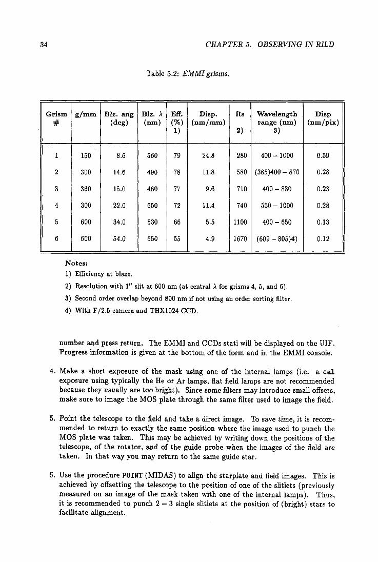
34 CHAPTER 5. OBSERVING IN RILD
Table 5.2: EMMI grisms.
Grisrn g/rnrn BIz. ang BIz. ,\ Eft'. Disp. Rs Wavelength Disp #
1
2
3
4
5
6
(deg) (nrn) (%) (nrn/rnrn) range (nrn) (nrn/pix) 1) 2) 3)
150 8.6 560 79 24.8 280 400 - 1000 0.59
300 14.6 490 78 11.8 580 (385)400 - 870 0.28
360 15.0 460 77 9.6 710 400 - 830 0.23
300 22.0 650 72 11.4 740 550 - 1000 0.28
600 34.0 530 66 5.5 1100 400 - 650 0.13
600 54.0 650 55 4.9 1670 (609 - 805)4) 0.12
Notes:
1) Efficiency at blaze.
2) Resolution with I" slit at 600 nm (at central ,\ for grisms 4,5, and 6).
3) Second order overlap beyond 800 nm if not using an order sorting filter.
4) With F /2.5 camera and THXI024 CCO.
number and press return. The EMMI and eeDs stati will be displayed on the UIF. Progress information is given at the bottom of the form and in the EMMI console.
4. Make a short exposure of the mask using one of the internal lamps (i.e. a cal exposure using typically the He or Ar lamps, flat field lamps are not recommended because they usually are too bright). Since some filters may introduce small offsets, make sure to image the MOS plate through the same filter used to image the field.
5. Point the telescope to the field and take a direct image. To save time, it is recommended to return to exactly the same position where the image used to punch the MOS plate was taken. This may be achieved by writing down the positions of the telescope, of the rotator, and of the guide probe when the images of the field are taken. In that way you may return to the same guide star.
6. Use the procedure POINT (MIDAS) to align the starplate and field images. This is achieved by offsetting the telescope to the position of one of the slitlets (previously measured on an image of the mask taken with one of the internal lamps). Thus, it is recommended to punch 2 - 3 single slitlets at the position of (bright) stars to facilitate alignment.

5.4. CALIBRATION EXPOSURES 35
7. If more than 150 punches are requested for one field, steps 2 and 3 above have to be repeated.
5.4 Calibration exposures
5.4.1 Bias and darks
CCDs have an electronic bias that can be evaluated by averaging several Os dark exposures and substracted from the science images to take it out. By using these exposures the observer can check the CCD readout noise and possible pick-up patterns in the electronic background. The dark exposures of the TEK2048 CCD (ESO No 36) show a few bright columns which divide out well. Should strong patterns appear on I SLOW I readout bias frames, call the NTT coordinator (93-50 in the paging system). At least one, but if possible more, long (at least 1 hour) dark exposures are useful to monitor the dark current of the CCD.
When the TEK CCD is read via a single amplifier (normally amp D), the conversion factor (9) is normally lADU = 1.35e-. The readout noise (um) measured during the commissioning was 5e- in slow mode. In fast read-out the £f is lADU = 5.7e- and the ron 8e-. In dual output (Sect. 5.3.4)the second amplifier (normally amp A) has a 9 of lADU = 1.4e- and a!2E of 6e- in slow read-out. In fast read-out the cf is lADU = 6.leand the ron = 8.5e-.
The dark current at l5loK is found to be '" 5e- /hr/pixel.
5.4.2 Flat field exposures
The linearity of the TEK2048 CCD No 36 has been measured in the laboratory and is found to be better than 0.6% over a range of 4 decades. The flat fields show variations in the QE of ±lO% d~e to the non-uniformity or defects in the coating.
The flat field characteristics of CCDs are wavelength dependent and therefore, for broadband imaging, the best results are obtained using sky flats. They can be done on the sky during morning and evening twilight. For broad-band filters this is possible for about 30 minutes around -120 twilight; narrow-band exposures can be done close to sunrise and sunset. Very accurate results in broad-band imaging are obtained by median filtering of the science images if they are poorly populated with stars and do not contain very extended sources. A list of sparsely populated fields is available in the control room. Sky flats are also recommended to determine the slit function for long-slit spectroscopy. There are also dome lamps that can be used to take dome flatfields; the night assistant or the introducing astronomer can assist the visitor in their use.
A calibration unit is mounted on the side of the adapter for flat fields in spectroscopy and wavelength calibration. The exposure times for flat fielding can be easily determined with a few test exposures. Typically they do not exceed a few seconds. Therefore start with a 1 second exposure, substract the bias level, and scale up the result. The count rates grisms at their blazes wavelengths obtained with the internal lamp for spectroscopy are
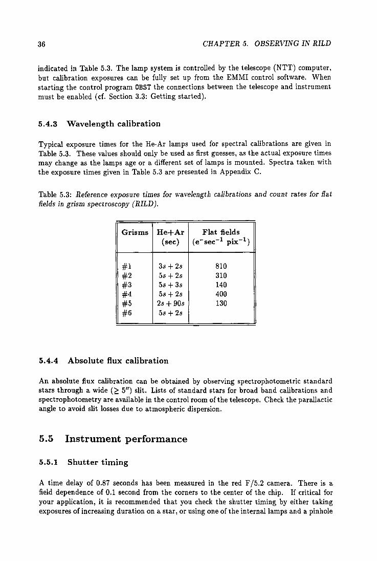
36 CHAPTER .5. OBSERVING IN RILD
indicated in Table 5.3. The lamp system is controlled by the telescope (NTT) computer, but calibration exposures can be fully set up from the EMMI control software. When starting the control program OBST the connections between the telescope and instrument must be enabled (d. Section 3.3: Getting started).
5.4.3 Wavelength calibration
Typical exposure times for the He-Ar lamps used for spectral calibrations are given in Table 5.3. These values should only be used as first guesses, as the actual exposure times may change as the lamps age or a different set of lamps is mounted. Spectra taken with the exposure times given in Table 5.3 are presented in Appendix C.
Table 5.3: Reference exposure times for wavelength calibrations and count rates for flat fields in grism spectroscopy (RILD).
Grisms He+Ar Flat fields (sec) (e-sec-1 pix-I)
#1 38 + 28 810 #2 58 + 28 310 #3 58 + 35 140 #4 55 + 28 400 #5 28 + .908 130 #6 55 + 28
5.4.4 Absolute flux calibration
An absolute flux calibration can be obtained by observing spectrophotometric standard stars through a wide (~ 5") slit. Lists of standard stars for broad band calibrations and spectrophotometry are available in the control room of the telescope. Check the parallactic angle to avoid slit losses due to atmospheric dispersion.
5.5 Instrument performance
5.5.1 Shutter timing
A time delay of 0.87 seconds has been measured in the red F /5.2 camera. There is a field dependence of 0.1 second from the corners to the center of the chip. If critical for your application, it is recommended that you check the shutter timing by either taking exposures of increasing duration on a star, or using one of the internal lamps and a pinhole
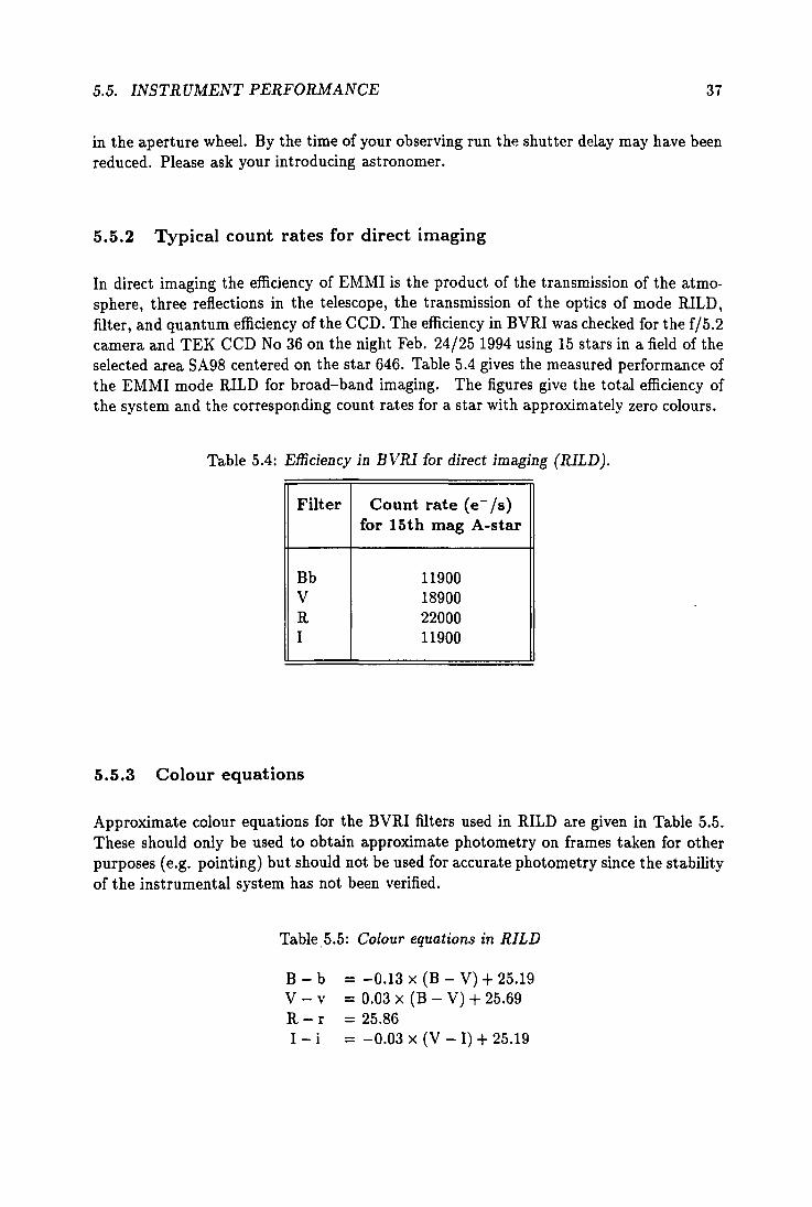
5.5. INSTRUMENT PERFORMANCE 37
in the aperture wheel. By the time of your observing run the shutter delay may have been reduced. Please ask your introducing astronomer.
5.5.2 Typical count rates for direct imaging
In direct imaging the efficiency of EMMI is the product of the transmission of the atmosphere, three reflections in the telescope, the transmission of the optics of mode RILD, filter, and quantum efficiency ofthe CCD. The efficiency in BVRI was checked for the f/5.2 camera and TEK CCD No 36 on the night Feb. 24/25 1994 using 15 stars in a field of the selected area SA98 centered on the star 646. Table 5.4 gives the measured performance of the EMMI mode RILD for broad-band imaging. The figures give the total efficiency of the system and the corresponding count rates for a star with approximately zero colours.
Table 5.4: Efficiency in BVRI for direct imaging (RILD).
Filter Count rate (e- Is) for 15th mag A-star
Bb 11900 V 18900 R 22000 I 11900
5.5.3 Colour equations
Approximate colour equations for the BVRI filters used in RILD are given in Table 5.5. These should only be used to obtain approximate photometry on frames taken for other purposes (e.g. pointing) but should not be used for accurate photometry since the stability of the instrumental system has not been verified.
Table 5.5: Colour equations in RILD
B-b V-v R-r I-i
= -0.13 x (B - V) + 25.19 = 0.03 x (B - V) + 25.69 = 25.86 = -0.03 x (V - I) + 25.19
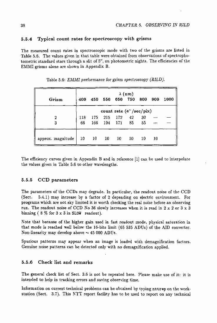
38 CHAPTER .5. OBSERVING IN RILD
5.5.4 Typical count rates for spectroscopy with grisms
The measured count rates in spectroscopic mode with two of the grisms are listed in Table 5.6. The values given in that table were obtained from observations of spectrophotometric standard stars through a slit of 5/1, on photometric nights. The efficiencies of the EMMI grisms alone are shown in Appendix B.
Table 5.6: EMMI performance for grism spectroscopy (RILD).
A (nm) Grism 400 450 550 650 750 800 900 1000
count rate (e- /sec/pix)
2 118 175 215 172 42 30 - -
3 66 166 194 171 85 55 - -
approx. magnHude 10 10 10 10 10 10 10
The efficiency curves given in Appendix B and in reference [IJ can be used to interpolate the values given in Table 5.6 to other wavelengths.
5.5.5 CCD parameters
The parameters of the CCDs may degrade. In particular, the readout noise of the CCD (Sect. 5.4.1) may increase by a factor of 2 depending on electric environment. For programs which are not sky limited it is worth checking the real noise before an observing run. The readout noise of CCD No 36 slowly increases when it is read in 2 x 2 or 3 x 3 binning ( 8 % for 3 x 3 in SLOW readout).
Note that because of the higher gain used in fast readout mode, physical saturation in that mode is reached well below the 16-bits limit (65 535 ADUs) of the AID converter. Non-linearity may develop above f'V 45 000 ADUs.
Spurious patterns may appear when an image is loaded with demagnification factors. Genuine noise patterns can be detected only with no demagnification applied.
5.5.6 Check list and remarks
The general check list of Sect. 3.6 is not be repeated here. Please make use of it: it is intended to help in tracking errors and saving observing time.
Information on current technical problems can be obtained by typing nttrep on the workstation (Sect. 3.7). This NTT report facility has to be used to report on any technical

5.5. INSTRUMENT PERFORMANCE 39
problem during your run. The operation staff will also use it to report on what they did to solve your problem.

Chapter 6
Observing in BIMG
6.1 Optical configuration
In the Blue Imaging mode (BIMG) the instrument works as a focal reducer at F /4. The optics in the blue channel is coated for high efficiency transmission in the region 300 nm to 500 nm. A filter wheel is mounted in the converging beam in front of the camera for doing imaging. The light path in this mode is illustrated in Figure 6.1. Spectroscopy in the blue arm is possible by using gratings. It requires a different configuration of the instrument which is described in Chapter 8: Observing in BLMD.
BIMG
Figure 6.1: Light path in BIMG mode of EMMI
40

6.2. INSTRUMENT SETUP 41
6.2 Instrument setup
The instrument setup is simply performed by selecting one position of the filter wheel. This is done in the user interface by going first to I Top menu I then choosing the BIM G
mode by clicking SIMG. After selecting the mode, the setup can be done by clicking the setup command SIMG Setups. A form appears on the screen that allows you to predefine instrument con guratlOns. Do not forget to focus the camera according to the EMMI temperature and the chosen filters. To define exposures click the command I SIMG exposures I and fill the form as described in Section 3.5: Defining and executing exposures.
6.2.1 Filters
Up to 8 filters can be mounted in the filter wheel. Blue filters are mounted in cells perpendicular to the optical axis. Information on the transmission curves and quality of the filters can be obtained by using the MIDAS context FILTERS. A list of standard EMMI blue filters is given in Table 6.1. Observers who wish to use other filters are reminded of the image quality requirements. U and B photometry should normally be done in the blue arm of EMMI, the red optics having a sharp cut-on at 390 nm due to the coating. The Bb filter is a blue filter intended for use in the red arm of EMMI. It is open towards the UV so its effective colour equation depends on EMMI and camera transmissions and CCD QE at '" 400 nm. A red filter used in the blue will cause some astigmatism. If a blue filter is used in the red arm, every object in the field produces a ghost which is about 5 magnitudes lower in brightness. Image anomalies are described in Chapter 11.
6.3 0 bserving
6.3.1 Focusing using through-focus sequences
Click the focus parameters bar of the BIMG mode Le. click SIMG Focus param.. A form will appear on the RAMTEK display. The parameters reqUIre are t e num er of focus steps (typically 7 - 9), the focus increment (step size, typically 10 - 30lLm), and the telescope offset in R.A. or Dec. (or both; typically 10"). The parameters for the instrument focus are also specified in this form. Here you must give the number of steps and the camera focus offset. foc type exposures use the current position of the telescope or camera focus as the value of the middle step of the sequence. Thus, if you want to start at any given focus value, you must position the focus to the value mid-way of the sequence. For example, if you want to start at -3.000 mm, the focus of the telescope should be positioned to -2.960 mm for 9 focus steps of 101Lm. The optimal focus may be derived using the procedure FOCUS. The use of that procedure is described in Appendix A. In order to average seeing effects do not use excessively short individual exposures ( < 20sec) for the focus sequences.
The focus in RILD with no filter or the R filter is the same as the BIMG focus with the B filter.

42 CHAPTER 6. OBSERVING IN BIMG
Table 6.1: EMMI filters for the blue arm
ESO Filter >'01 ~>. {nm} Peak efficiency Cell type Focus offsets FWHM (%) (arm)
587 He I 448.0/5.0 55 R -22 588 He II 469.2 6.6 72 B 97 589 om/O 501.4 5.6 64 2 590 om /3000 505.7 6.4 52 +7 591 o III /6000 511.2 6.1 69 -5 592 o III I 9000 516.0/6.3 68 26 593 o III / 12000 521.1/6.7 66 0 594 om / 15000 526.0/6.6 65 -3 602 U 354/54 67 B 40 603 B 423/94 65 B 0 643 BG382mm 480/320 97 644 GG3753mm cut. on 370 98 645 OG530 3mm cut on 530 98 0 647 Ne V 342.7/8.2 42 648 o II I 0 373.0/6.7 92 649 o II / 5000 379.9/6.7 45 650 o II /10000 385.8/6.9 43 651 o II /15000 392.4/7.6 40 652 He II 469.6/7.3 61 658 EUV (UGll/5) 328/75 71
6.3.2 Checking the seeing
The seeing can be checked on images taken in BIMG by clicking the field I seeing I that appears on top of the MIDAS display window (Sect. 5.3.3, and Appendix A). The image scale is read in the header of the displayed image and does not need to be specified. The seeing measured outside the telescope by the seeing monitor can be displayed on the workstation by typing meteomonitor (Sect. 4.4).
6.3.3 Pointing and guiding
The pointing of the NTT is of the order of 2 arcsec rms. Guiding the telescope is normally done by centering a star on one of the two guides probes and starting the autoguider.
6.3.4 Direct imaging
The camera on the blue arm of EMMI is at F / 4 and the detector presently used is a TEK CCD of 10242 pixels, 241lm in size (ESO No 31). This gives a scale of 0.37 arcsec/pixel and a field of view of 6.2 x 6.2 arcmin.

6.4. CALIBRATION EXPOSURES 43
6.4 Calibration exposures
6.4.1 Bias and darks
It is not safe to assume the bias to be always a scalar and therefore it is recommended to take many bias exposures.
It has proven to be extremely difficult to isolate the CCD electronics from electrical interference from components in the NTT adapters/derotators. Therefore to some extent, the EMMI CCDs show pick-up patterns in the electronic background (the bias). This noise is minimized in SLOW readout mode, but may he rather strong in FAST readout frames. The patterns are not stable, but change from one exposure to the next, so it is difficult to remove them completely by substracting bias frames. However, some reduction can be achieved and, therefore, it is recommended to take a good number of bias frames throughout the observing run. Should strong patterns (Le. more than a few ADUs) appear on SLOW readout bias frames, call the NTT coordinator (93-50). Note that spurious patterns are introduced if images are displayed with demagnification factors.
At least one, but preferably more, long (1 hour) dark exposures should be taken to monitor the dark current and any exposure dependent features.
The normal values for the TEK1024 CCD (ESO No 31) are as follows. Conversion factor: 1ADU = 3.3e-. Read-out noise N 7e- rms. The dark current is N 8e- /pixel/hr at 166 K. There are approximately 8 small traps extending over less than 20 pixels.
6.4.2 Flat fields exposures
The linearity of CCD No 31 is very good up to 160000 e- /pixel. The most accurate results for flat fields in broad band imaging are obtained using sky flats. This may be achieved by median filtering of the science images if they are not too densely populated with stars and contain no very extended objects, or by doing multiple exposures of sparsely populated fields, with spatial offsets. A list of such fields is available in the control room. An other approach is to use morning and evening twilight (N half an hour when the sun elevation is N -120. There are also dome lamps that can be used to take flat fields in the dome. The introducing astronomer can assist the visitor in their use.
6.4.3 Absolute flux calibration
Lists of standard stars for calibrations of broad band images with CCDs are available in the control room of the telescope.

44 CHAPTER 6. OBSERVING IN BIMG
6.5 Instrument performance
6.5.1 Shutter timing
A time delay of 0.80 seconds has been measured for the shutter in the blue F / 4 camera. If critical for your application, it is recommended that you check the shutter timing by
. either taking exposures of increasing duration on a star, or using one of the internal lamps and a pinhole in the aperture wheel.
6.5.2 Typical count rates
In blue imaging the efficiency of EMMI is the product of the transmission of the atmosphere, three reflections in the telescope, the transmission of the blue coated optics of mode BIMG, filter, and quantum efficiency of the CCD. The efficiency in Band U was checked for the F /4 camera and TEK CCD No 31 in 1993. The count rates in e- /sec deduced for a 15th magnitude A star with approximately zero colour are U: 2 200, B: 16900 at unit airmass.
6.5.3 Colour equation
An approximate colour equation beween u and b has been obtained from standard stars. The data for CCD No 31 give the following relation:
U - u = +0.01 (u - b)+ 23.34
6.5.4 Check list and remarks
A general check list for observations can be found in Sect. 3.6. Please make use of it: it is intended to help in tracking errors and saving observing time.
Remember that you can get information on current technical problems by typing nttrep on the workstation (Sect. 3.7). This NTT report facility will have to be used to report on any technical problem during your observing run. The operation staff will also use it to report on technical solutions.
To get information on the seeing and other meteorological local parameters type meteomoni tor
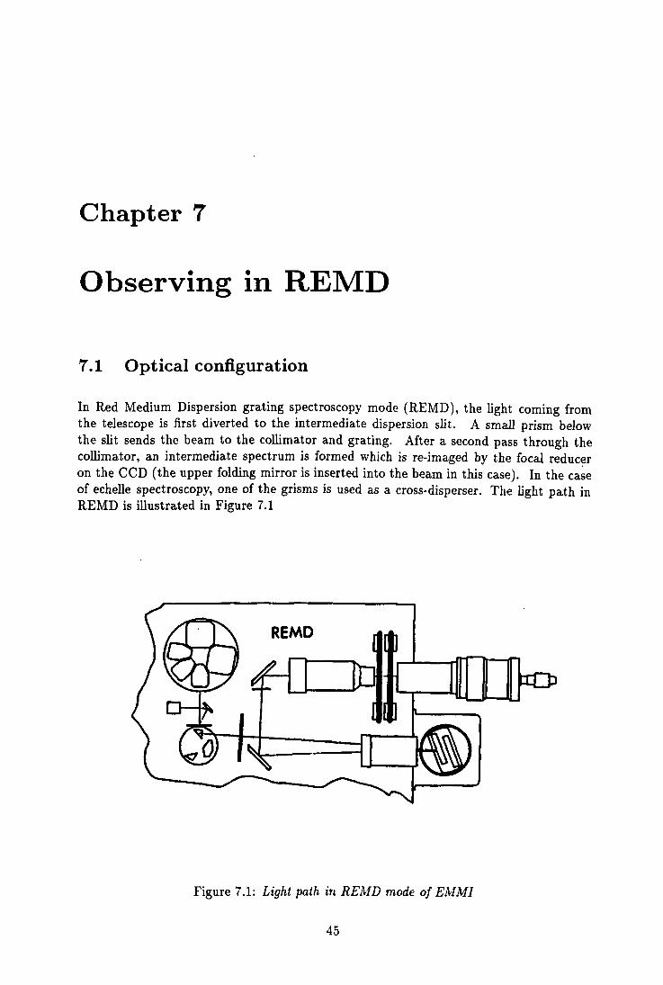
Chapter 7
Observing in REMD
7.1 Optical configuration
In Red Medium Dispersion grating spectroscopy mode (REMD), the light coming from the telescope is first diverted to the intermediate dispersion slit. A small prism below the slit sends the beam to the collimator and grating. After a second pass through the collimator, an intermediate spectrum is formed which is re-imaged by the focal reducer on the CCD (the upper folding mirror is inserted into the beam in this case). In the ca~e of echelle spectroscopy, one of the grisms is used as across-disperser. The light path in REMD is illustrated in Figure 7.1
REMD
Figure 7.1: Light path in REMD mode of EMMI
45
46 ClIAPTER 7. OBSERVING IN REMD
7.2 Instrument setup
To prepare a setup using the EMMI interface first go to 1 Top menu 1 and select the REMD
mode by clicking 1 REMD I. The setup can then be done after clicking the setup command 1 REMD setups I. A form appears on the screen. An instrumental configuration is predefined by selecting a slit width and decker, plus either a grating and a central wavelength, or an echelle grating and a cross dispersing grism, or also an echelle grating and a narrow band filter. Only grisms marked CD (in positions 6 and 7) are properly mounted for usage as cross disperser. An order sorting filter will be additionally needed when the next higher or lower order of a non echelle grating overlaps with the wavelength range in which the detector has significant sensitivity. The focus of the instrument should be calculated from the REMD temperature relation, which is given in the printed setup form (see Figure 3.1 ), and entered in the corresponding field of the instrument setup, or also an echelle grating and a narrow band filter. Filter offset, as indicated in the RILD field of the setup form, must be added.
7.2.1 Slit
The slit width in the intermediate dispersion modes can be continuously adjusted between o and 9 arcsec. The slit length is 6 arcmin. A movable decker is permanently mounted on the slit. The medium dispersion slit is oriented East-West. The same slit is also used in modes BLMD and DIMD. It can be oriented in a different direction (e.g. parallel to the parallactic angle to minimize slit losses due to atmospheric dispersion) by rotating the adapter and instrument at the beginning of an exposure. Note that different slits are used in RILD. They are mounted in a slit wheel. A slit selected in RILD is oriented North-South.
7.2.2 Gratings
Four gratings are available in mode REMD. Their properties are described in Table 7.1.
7.2.3 Echelle gratings
Two echelle gratings (#9 and # 10) are presently offered. They can be used in combination with a cross-dispersing grism to obtain data in an echelle format. Grisms # 3 and # 4 are used with the echelle grating # 9, grisms # 3, #4, # 5 and # 6 with the echelle grating # 10. The properties of the echelle spectra obtained using different cross-dispersers are given in the EMMI & SUSI manual Version No 1 (September 1992). A third echelle grating has recently been tested. Its properties and availability will be announced in a future issue of The Messenger.
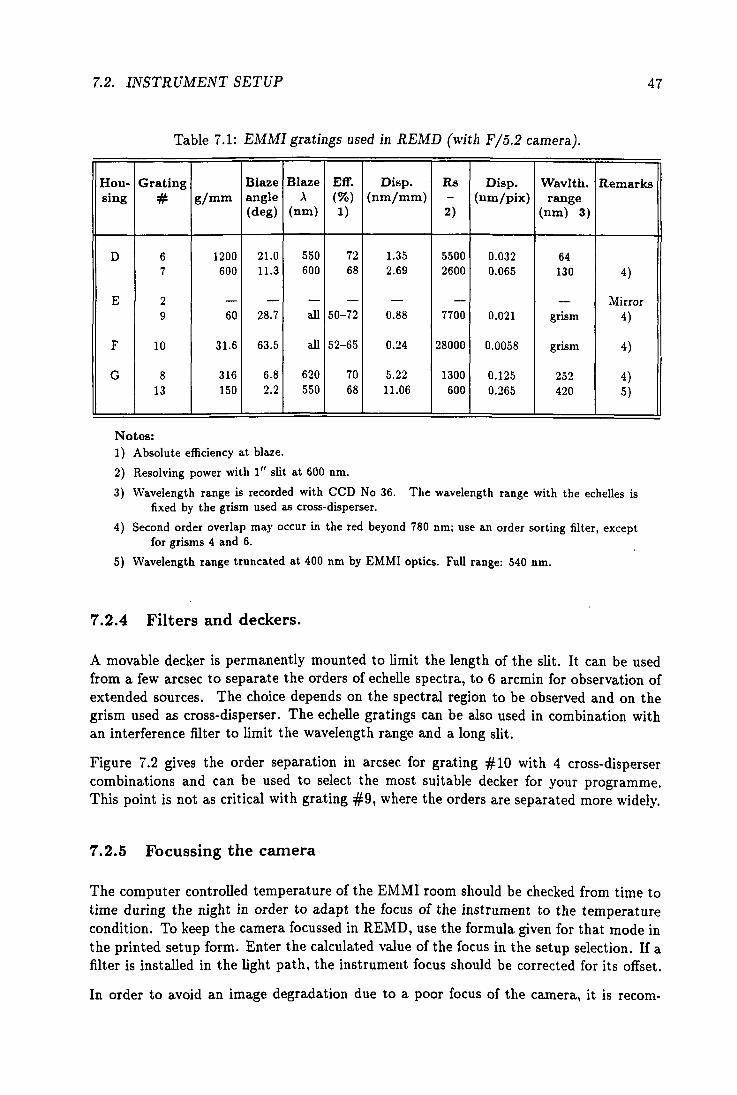
7.2. INSTRUMENT SETUP 47
Table 7.1: EMMI gratings used in REMD (with F/5.2 camera).
Hou- Grating Blaze Blaze Eft'. Disp. Rs Disp. Wavlth. Remarks sing # g/mm angle ..\ (%) (nm/mm) - (nm/pix) range
(deg) (nm) 1) 2) (nm) 3)
D 6 1200 21.0 550 72 1.35 5500 0.032 64 7 600 11.3 600 68 2.69 2600 0.065 130 4)
E 2 - - - - - - - Mirror 9 60 28.7 all 50-72 O.B8 7700 0.021 grism 4)
F 10 31.6 63.5 all 52-65 0.24 28000 0.0058 grism 4)
G 8 316 6.8 620 70 5.22 1300 0.125 252 4) 13 150 2.2 550 68 11.06 600 0.265 420 5)
Notes: 1) Absolute efficiency at blaze.
2) Resolving power with I" slit at 600 nm.
3) Wavelength range is recorded with CCD No 36. The wavelength range with the echelles is fixed by the grism used as cross-disperser.
4) Second order overlap may occur in the red beyond 780 nm; use an order sorting filter, except for grisms 4 and 6.
5) Wavelength range truncated at 400 nm by EMMI optics. Full range: 540 nm.
7.2.4 Filters and deckers.
A movable decker is permanently mounted to limit the length of the slit. It can be used from a few arc sec to separate the orders of echelle spectra, to 6 arcmin for observation of extended sources. The choice depends on the spectral region to be observed and on the grism used as cross-disperser. The echelle gratings can be also used in combination with an interference filter to limit the wavelength range and a long slit.
Figure 7.2 gives the order separation in arcsec for grating #10 with 4 cross-disperser combinations and can he used to select the most suitable decker for your programme. This point is not as critical with grating #9, where the orders are separated more widely.
7.2.5 Focussing the camera
The computer controlled temperature of the EMMI room should be checked from time to time during the night in order to adapt the focus of the instrument to the temperature condition. To keep the camera focussed in REMD, use the formula given for that mode in the printed setup form. Enter the calculated value of the focus in the setup selection. If a filter is installed in the light path, the instrument focus should be corrected for its offset.
In order to avoid an image degradation due to a poor focus of the camera, it is recom-
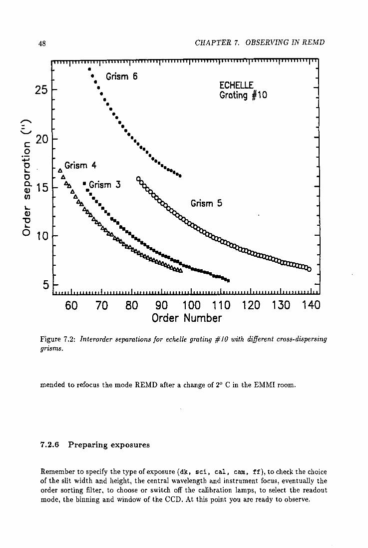
"...... -~
c: 0 .-+" 0 ~
0 a. Q.) en ~
Q.)
"0 L-
0
48 ClIAPTER 7. OBSERVING IN REMD
• • Grism 6 • ECHELLE 25 • • Grating #10 • • • • e • • •
20 •• e. e. ·e 6. Grism 4 6.
15 ~ • Grism 3 6. • 6. • • At. •• , ... ', .....
10
5
60 70 80
•• e. ... ••• Grism 5
90 100 110 120 130 140 Order Number
Figure 7.2: Interorder separations for echelle grating #10 with different cross-dispersing grisms.
mended to refocus the mode REMD after a change of 2° C in the EMMI room.
7.2.6 Preparing exposures
Remember to specify the type of exposure (dk, sci, cal, cam, ff), to check the choice of the slit width and height, the central wavelength and instrument focus, eventually the order sorting filter, to choose or switch off the calihration lamps, to select the readout mode, the binning and window of the CCD. At this point you are ready to observe.

7.3. OBSERVING 49
7.3 0 bserving
7.3.1 Focussing the telescope
The focus of the telescope in REMD is the same as in the imaging mode of the red arm (RILD). More precisely, if the telescope was focussed on RILD images and the camera focus in that mode was set according to the temperature in RILD, then the telescope is focussed on the REMD slit. The telescope focus can be determined using the focus wedge or a through-focus sequence, both in RILD. This is done in the user interface by going first to I Top menu I then chosing the RILD mode by clicking I RILD I. A setup can
be done by clicking I RILD Setups ,. Select the focus wedge in this setup, enter the focus corresponding to the temperature of the camera. in RILD (the temperature formulae are given in the printed setup form, e.g. Figure 3.1). The procedure of focussing with the focus wedge is described in Chapter 5: Observing in RILD (Sect. 5.3.1). Through-focus sequences can be used by clicking I RILD focus param., and following the same procedure as described in Chapter 6: Observing in BIMG (Sect. 6.3.1). To obtain REMD spectra the camera will have to be focussed according to the temperature in that mode.
7.3.2 Pointing using the slit viewer
Acquisition of the target for red medium dispersion spectroscopy is normally done with the intensified slit-viewer TV. The scale of the transfer optics is such· that 1 arcsec :::::: 2.2 TV lines. The useful field is approximately 2.5 x 6 arcmin. The limiting magnitude has been measured to be around 19 in the red-visual with seeing of 1 arcsec in a dark night, without frame integration. Note that especially during bright nights, integrating is of limited use because the background and noise are also amplified.
The default orientation on the viewer monitor is east to the bottom, north to the right. The medium dispersion (MD) slit is oriented east-west, but the dispersion is still parallel to the CCD rows. A mirror projects the light from the telescope on the slit.
In the REMD mode the guiding, either visually or with the autoguider, can also be done on the image of the field as reflected off the slit jaws and recorded by the intensified slit-viewer TV.
7.3.3 Pointing a faint object
For pointing objects which cannot be seen on the slit viewer one has to use the apparent position of the MD slit in imaging mode. That apparent position is obtained by centering a relatively bright star on the slit using the slit viewer and taking a short exposure in RILD (Sect. 5.3.4). Next, take an image of the faint object in RILD and move it to the apparent coordinates of the slit, previously measured, using the procedure POINT (Appendix A). Then switch back to grating spectroscopy. If the first offset to be applied exceeds "" 20", take a second direct image to check the accuracy of the centering.
To verify the position of an object on the MD slit before starting an exposure in REMD ,
50 CHAPTER 7. OBSERVING IN REMD
or simply to inspect the field, one can move the mirror which reflects the light to the slits by typing from the terminal the command, OBST > EMMI > MIRR REMD. This can also be
done using the soft-key I ~~~~ I on the OBST console (not the Ramtek UIF). To remove the mirror one must type OBST > EMMI > MIRR RILD.
The seeing can be checked on RILD exposures with exposure time> 20 sec (Sect. 5.3.3).
7.4 Calibration exposures
7.4.1 Bias and darks
The electronic bias level can be evaluated by averaging several short dark exposures. The normal readout noise of the TEK2048 CCD (ESO No 36) is 5e- rms when it is read in SLOW mode with its sandard conversion factor of 1ADU = 1.35e-. Pick-up patterns due to the electric environment are minimized in SLOW mode. Long dark exposures are useful to monitor the dark current. The dark current of CCD No 36 is found to be '" 5e- /pixel/hr at 151°K. More information on the CCD camera can be found in Sect. 5.3.4 and 5.5.5.
7.4.2 Wavelength calibrations and flat fields
Flat field exposures can be obtained by using the internal lamp of the calibration unit or lamps installed on the top ring of the telescope. Median filtered flat fields can be used to correct for pixel to pixel variations and for the echelle blaze function. They can also be used in the MIDAS echelle reduction to fit the echelle orders. The exposure times for flat fields with the internal lamp are long. For the echelle gratings # 9 and # 10 the top ring lamps, which are more powerful, should be prefered . Flat fields must be obtained in the same readout mode and binning as the science exposures. Note that in fast readout mode saturation is reached faster than in slow mode because of the higher gain factor. In that mode, physical saturation of the CCD occurs before saturation of the AID converter (Sect. 5.5.5). Depending on the resolution of the spectrograph configuration the lines from He+Ar or ThAr lamps can be used for wavelength calibration. Table 7.2 gives Ar approximate exposure times for two gratings. Spectra obtained with these exposures times are shown in Appendix D.
In cross-dispersed echelle spectroscopy with CDs # 3 and #5. the recorded flat fields have a very different level at the blue and the red ends of the spectral range, due to the combination of the response curve of EMMI and of the gradient of the flat field lamps. It is difficult to obtain good flat fields for the blue end of these echelle spectra. Many flat field exposures must be taken.
An elastic flexure behaviour due to the rotation of the adapter has been registered in mode REMD for the F /5.2 camera. The peak to peak variation in the X direction (the actual direction of the dispersion) is 1.8 pixel for a rotation of 1800
• The curve shows that there is some hysteresis. For programs in which wavelength calibration is very critical, the calibration should be taken at the same mean rotator angle as the exposure, and that position should be reached by rotating the adapter in the same direction as the exposure.

7.5. CHECK LIST AND REMARKS 51
In that case please check the rotation parameters of the adapter on the telescope UIF.
Table 7.2: Reference exposure times for wavelength calibrations and count rates for flat fields in REMD.
Gratings He+Ar Flat fields (sec) e- sec-1 pix-1
# 6 @550 nm o + 2408* 9
# 7 @600 nm o + 2408* 35
* Ar exposure.
7.4.3 Absolute flux calibration
Observations of spectrophotometric standard stars can be used to obtain absolute flux calibrations of the spectra acquired with a given setup. A large slit width (~ 5") should be used for flux calibration. In order to minimize slit losses due to atmospheric dispersion, the slit should be oriented parallel to the parallactic angle. The parallactic angle is available from the Telescope Control System (TCS). Please ask the night assistant. A List of standard stars for spectrophotometry is available in the control room of the telescope.
7.5 Check list and remarks
In addition to the main check list given in Sect. 3.6, we encourage you to check particularly the following points:
1. Is the central wavelength properly set?
2. Is the grism used in combination with the echelle grating properly selected?
3. Is the decker length adequate for separating the orders but, for faint objects, also to estimate the sky background?
4. Is the camera properly focussed? If a filter is used, its offset has to be taken into account.
5. Is the slit width chosen for the required resolution correctly switched in?
6. Is there any error message on the EMMI terminal LU: 53? Check this monitor regularly because messages may scroll off the page and, therefore escape notice.
7. Check the readout mode, window and binning of the detectors.
8. Is the exposure time adapted to the slit width and seeing?

52 CHAPTER 7. OBSERVING IN REMD
9. Is the rotator range sufficient for your long exposure?
10. Mirror out?
Remember also that the seeing measured by the external seeing monitor can be easily obtained by typing meteomoni tor on the workstation (e.g. Sect. 4.4).
Technical problems have to be reported through the NTT report system by typing nttrep on the workstation (Sect. 3.7 ) and filling in the self explanatory form. Remember that a good diagnostic requires an accurate description of the symptoms.

Chapter 8
Observing in BLMD
8.1 Optical configuration
In Blue Medium Dispersion grating spectroscopy (BLMD), like in REMD, the light corning from the telescope is first diverted to the intermediate dispersion slit. A small prism below the slit sends the beam to the blue collimator and grating unit. After a second pass through the collimator, an intermediate spectrum is formed which is re-imaged on the CCD. Echelle spectroscopy is not possible in that mode. The light path in BLMD is illustrated in Figure 8.1
BLMD
Figure 8.1: Light path in BLMD mode of EMMI
53

54 CIL1PTER 8. OBSERVING IN BLMD
8.2 Instrument setup
To prepare a setup in BLMD mode using the EMMI interface first go to I Top menu I and
select the BLMD mode by clicking 1 BLMO I. After selecting the mode, the setup can be done by clicking I BLMO setups I. An instrumental configuration is predefined by selecting a slit width and length plus a grating and central wavelength. The focus of the instrument calculated from the temperature relation in BLMD (given in the printed setup form, e.g. Figure 3.1) should be entered in the corresponding field of the instrument setup. It has been found to be critical in that mode. After you fill the form, hit RETURN and wait for the audible signal before preparing exposures.
8.2.1 Slit
The slit in the intermediate dispersion BLMD mode is the same as in REMD (Sect. 7.2.1). Its width can be continuously adjusted between 0 and 9 arcsec. The maximum slit length is 6 arcmin. A moveable decker can be used to restrict the slit length. The slit is oriented east-west, but can be oriented in a different direction by rota.ting the instrument at the beginning of an exposure.
8.2.2 Gratings
There are 5 gratings available in mode BLMD. Their properties are described in Table 8.1. They are permanently mounted two by two in 3 housings. The user has the choice of 2 gratings (Le. one housing) in a given observing night. Note that two other gratings can be mounted in the red arm for grating (or echelle) spectroscopy in REMD.
8.2.3 Focussing the camera
The focus of the instrument in BLMD mode is very sensitive to the temperature. In order to avoid a degradation of the spectra it is recommended to refocus the camera in mode BLMD after a temperature change of 10 C in the EMMI room. The relationship between temperature and instrument focus is given in the printed setup form (see e.g. Figure 3.1). The controlled temperature of the EMMI room should be continuously checked during the night in order to adapt the focus of the instrument to the temperature condition.
The blue collimator is not perfectly apochromatic so a focus correction will slightly improve the resolution at the extremes of the wavelength range. Table 8.2 gives the focus correction as a function of wavelength with respect to the value given by the temperature equation specified in the set-up form. The best overall focus is obtained at 360 nm.
8.2.4 Preparing an exposure
Select I BLMO exposures 1 by clicking the mouse and prepare exposures. Remember to specify the type of exposure (dk. sci. cal, cam, ff), check the choice of the slit width

8.3. OBSERVING
Table 8.1: EMMI gratings used in BLMD
Hou- Grating g/mm Blaze Blaze Eff. Disp. Rs Disp. Wavlth. Remarks sing # angle >. (%) (nm/mm) - (nm/pix) range
(deg) (nm) 1) 2) 3) arm 4) (nm)
A 1 - - - - - - - -4 300 3.6 400 72 7.2 840 0.173 170
B 3 1200 13.9 380 65 1.75 3400 0.042 46 5 158 1.8 370 72 15 400 0.360 250
C 11 3000 350 -50 0.61 11000 0.015 12 12 600 350 -65 3.78 1700 0.091 75
Notes: 1) Absolute efficiency at blaze.
2) With F /4 camera.
3) Resolving power with 1" slit at 400 nm.
4) Wavelength range is recorded with F /4 camera and TEKI024 ccn.
Table 8.2: BLMD focus correction as a function of wavelength
,\ (nm) 300 320 340 360 380 400 440 480 520 Corr (steps) -74 -63 -42 -23 -9 0 0 -18 -52
Mirror
55
and height, the central wavelength of the chosen grating, the instrument focus, choose or switch off the calibration lamps, select the readout mode, the binning and window of the CCD.
8.3 0 bserving
8.3.1 Focussing the telescope
The objective is to have the telescope focussed on the medium dispersion slit. This is achieved when, the blue camera being focussed according to the temperature relation in BLMD and the red camera being focussed according to the temperature relation in RILD, the telescope is in focus for the RILD mode. The telescope can be focussed in RILD by using the focus wedge. This is done in the user interface by going first to 1 Top menu I. Next, in the chosen 1 RILD I mode, click RILD Setups and prepare a setup including the focus wedge without filter. Then follow t e escnptlOn on focussing with the focus wedge given in Chapter 5: Observing in RILD (Sect. 5.3.1). The telescope can also be focussed in RILD using a through-focus sequence. In RILD mode click I RrLD Focus param.1 and

56 CHAPTER 8. OBSERVING IN BLMD
prepare a focus sequence as described in Sect. 6.3.1: Focussing using a through-focus sequence in Chapter 6.
8.3.2 Pointing using the slit viewer
Pointing brigth objects
Acquisition of the target in blue medium dispersion spectroscopy is normally done with the intensified slit-viewer TV as in REMD. The default orientation on the viewer monitor is east to the bottom, north to the right. The medium dispersion slit is oriented east-west. In the spectra the dispersion is parallel to the CCD rows. The guiding, either visual or using the au toguider, can also be done on the image of the field as reflected off the slit jaws and recorded by the intensified slit-viewer TV. The slit can be oriented by giving an angle offset to the rotator.
Pointing fainter objects
Two different mirrors project the light from the telescope on the slit depending on whether you work in the blue (BLMD) or red (REMD). The red mirror is a better match to the response of the TV and hence permits usually to see fainter objects. When the instrument is properly aligned, at least in the central part of the field there is a perfect overlap between the images of the slit in red and blue. This permits to use the red mirror to point an object for a blue spectrum.
8.3.3 Pointing objects not visible on the TV camera
For pointing objects which cannot be seen on the slit viewer one has to use the apparent· position of the medium dispersion slit in imaging mode (Sect. i.3.3). The apparent position of the slit is measured by taking a short exposure in mode RILD (Sect. 5.3.4) of a star previously centered on the slit. Next, take an image of the faint object and move it to the apparent position of the slit using the procedure POINT (Appendix A). Then switch back to grating spectroscopy. If the offset is larger than "" 20", check the centering by taking a second direct image.
8.4 Calibration exposures
8.4.1 Bias and darks
The normal readout noise ofthe TEK1024 CCD (ESO No 31 ) is 7 e- rms when it is read in SLOW mode with a conversion factor of 1 ADD = 3.3 e-. Pick-up patterns due to the electric environment migth be visible in FAST readout. They are minimized in SLOW mode (sect. 6.4.1). The electronic bias level, noise and possible structures can be evaluated
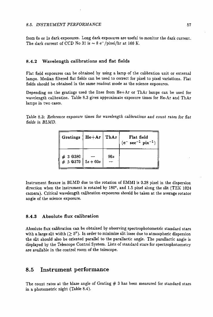
8.5. INSTRUMENT PERFORMANCE 57
from Os or Is dark exposures. Long dark exposures are useful to monitor the dark current. The dark current of CCD No 31 is I'V 8 e- /pixel/hr at 166 K.
8.4.2 Wavelength calibrations and flat fields
Flat field exposures can be obtained by using a lamp of the calibration unit or external lamps. Median filtered flat fields can be used to correct for pixel to pixel variations. Flat fields should be obtained in the same readout mode as the science exposures.
Depending on the gratings used the lines from He+Ar or ThAr lamps can be used for wavelength calibration. Table 8.3 gives approximate exposure times for He-Ar and ThAr lamps in two cases.
Table 8.3: Reference exposure times for wavelength calibrations and COUllt rates for fIat fields in BLMD.
Gratings He+Ar ThAr Flat field (e- sec-1 pix-1 )
# 3 @380 - 90s # ,5 @370 5s + 60s -
Instrument flexure in BLMD due to the rotation of EMMI is 0.28 pixel in the dispersion direction when the instrument is rotated by 180°, and 1.5 pixel along the slit (TEK 1024 camera). Critical wavelength calibration exposures should be taken at the average rotator angle of the science exposure.
8.4.3 Absolute flux calibration
Absolute flux calibration can be obtained by observing spectrophotometric standard stars with a large slit width (;::: 5"). In order to minimize slit losse due to atmospheric dispersion the slit should also be oriented parallel to the parallactic angle. The parallactic angle is displayed by the Telescope Control System. Lists of standard stars for spectrophotometry are available in the control room of the telescope.
8.S Instrument performance
The count rates at the blaze angle of Grating # 3 has been measured for standard stars in a photometric night (Table 8.4).

58 CHJ!PTER 8. OBSERVING IN BLMD
Table 8.4: EMMI performance for grating spectroscopy in BLMD.
Grating .x Count rate Approx. mag. (e- /sec/pix) of LTT 9239
#3 380 65 13.2
8.6 Check list
In addition to the main check list given in Sect. 3.6, the following points are important:
1. Is the central wavelength properly set?
2. Is the slit width chosen for the required resolution correctly switched in ?
3. Is the camera properly focussed? It should be refocussed after a temperature change of more than 10 C.
4. Is the slit oriented parallel to the parallactic angle (to minimize atmospheric losses)?
5. Remember that the seeing measured at the seeing monitor can be obtained by typing meteomoni tor at the workstation.
6. Is the current exposure time adapted to the slit width and seeing?
7. Is the rotator range left sufficient for the exposure time?
8. Check the EMMI monitor LV: 53 regularly because error messages displayed on this terminal may scroll off the page and escape notice.
9. Is mirror out?
Finally if you have technical problems which you mayor may not have been able to solve, fill in the computer based night report. Type nttrep on the workstation terminal and follow the self explanatory interface (see e.g. Sect. 3.7).
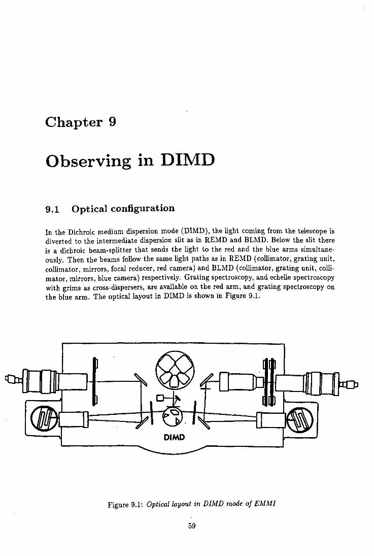
Chapter 9
Observing in DIMD
9.1 Optical configuration
In the Dichroic medium dispersion mode (DIMD), the light coming from the telescope is diverted to the intermediate dispersion slit as in REMD and BLMD. Below the slit there is a dichroic beam-splitter that sends the light to the red and the blue arms simultaneously. Then the beams follow the same light paths as in REMD (collimator, grating unit, collimator, mirrors, focal reducer, red camera) and BLMD (collimator, grating unit, collimator, mirrors, blue camera) respectively. Grating spectroscopy, and echelle spectroscopy with grims as cross-dispersers, are available on the red arm, and grating spectroscopy on the blue arm. The optical layout in DIMD is shown in Figure 9.1.
DIMD
Figure 9.1: Optical layout in DIMD mode of EMMI
59

60 CHAPTER 9. OBSERVING IN DIMD
9.2 Instrument setup
In the dichroic mode there are two light paths, i.e. two configurations one for the red arm and one for the blue arm. To prepare a DIMD setup using the EMMI interface, first go to Top menu, select the DIMD mode by clicking I DIMD I and reach the setup form by clicking
DIMD Setups. The configurations for the blue path and for the red path are prepared In t e same set up form. The fields are described in the order in which they appear in the UIF. The first two fields are for the blue and the red gratings, for which the central wavelength and number are entered. Then there are the below-slit filters which usually are left empty for observations as presently also are the ADCS and ADCC. Filters can be selected in the blue path and the red path, and a grism in the red path. Then there are the fields for the slit width, in arcsec, and the slit length (decker) also in arcsec. Finally the values of the instrument focuses are entered for the blue and the red cameras.
9.2.1 Slit
The slit which is used in the dichroic mode is the same as in Red Medium Dispersion mode (Chapter 7) and in Blue Medium Dispersion mode (Chapter 8).
9.2.2 Blue and red gratings and echelles
Using the dichroic mode does not introduce limitations in the choice of gratings and echelles as compared with the REMD and the BLMD modes. The same grisms are used as cross-dispersers of the echelle gratings as in REMD. We refer to Chapters 7 (REMD) and 8 (BLMD).
9.2.3 Exposure definition
Select DIMD Exposures by clicking the mouse. Define two consecutive exposures one for the re pat an one for the blue path. They are not necessarily of the same time since the optimal exposure times for a given object may be very different in BLMD and REMD. It is possible to take several exposures in an arm and one in the other. Remember that starting from the dichroic beam splitter there are two light paths, two shutters, two cameras and detectors. Specify the parameters for the two CCDs (readout modes, binnings and windows).
9.3 0 bserving
9.3.1 Focussing the telescope
Focussing the telescope can be made in RILD mode by using a focus wedge. The camera in RILD has to be focussed according to the temperature relation of that mode. The method

9.4. INSTRUMENT PERFORMANCE 61
is fully described in Sect. 5.3.1. If you wish to focus the telescope using a throughfocus sequence, you can also use the RILD mode and follow the procedure described in Sect. 6.3.1.
9.3.2 Focussing the blue and red cameras
To focus the cameras in DIMD, first calculate the focuses using the temperature relations of the REMD and the BLMD modes for respectively the red and the blue cameras. Then two offsets, which take into account the differences in light path introduced by the beam splitter, are added to these values. These offsets are indicated at the end of the EMMI optical setup form (Fig. 3.1.). Finally, if a filter is introduced in a beam, the corresponding camera focus has to be corrected also for the filter offset.
The temperature of the EMMI room is critical to avoid degradation of the spectra. The blue camera should be refocussed after a change of 10 C and the red camera after a change of 20 C.
9.3.3 Pointing using the slit viewer
The acquisition of a target in DIMD mode is made using the same intensified TV camera as in REMD and BLMD. The slit being the same as in these modes the pointing procedure is the same as described in Sect. 7.3.2 and Sect. 8.3.2.
9.4 Instrument performance
The overall efficiency of EMMI in DIMD mode as a function of wavelength is shown in Figure 2.3 . That curve only includes the transmission of the EMMI optics. By comparison of the efficiencies with and without beam splitter, the DIMD-to-REMD ratio in the red arm is of the order of 87% at 650 nm and the DIMD-to-BLMD ratio in the blue arm is '" 80% at 400 nm.
Flexures problems encountered in REMD are also relevant for observations in the dichroic mode. From tests performed on April 13, 1994, we suggest to follow the recommendations given in Sect. 7.4.2.
The use of the beam-splitter introduces a disalignment of the image of the slit on the CCDs, that is the slit no longer appears parallel to the CCD columns, contrary to what it does in REMD and BLMD.
The dichroic prism shows large variations in the polarization perpendicular to the slit. Efficiency variations normally flat field out for non polarized objects. It is not recommended to use the dichroic prism on polarized objects. The region with the highest polarization is between 400 and 480 nm.

· Chapter 10
Observing with SUSI
The Superb Seeing Imager (SUSI) is physically distinct from EMMI but complements its observing capabilities. A supporting plate is mounted on the adapter of the N asmyth A focus of the NTT. On the plate, a mirror with 3 positions is mounted. The first position sends the light to SUSI, the second feeds an IR camera (not available), and the third position is free for the operation of IRSPEC. A CAD view of the assembly (also called the Direct -Imaging Facility, DIFA) is presented in Figure 10.1. Between the diagonal mirror and the CCD is a filter wheel with 8 positions.
NTT Inttrfact fllftgt
Figure 10.1: CAD drawing of SUSI identifying its major components. The second dewar shown in the figure corresponds to an IR array camera.
62

10.1. SUSI FILTERS 63
SUSI uses a TEK CCD (ESO #25) with 1024 x 1024 pixels of 241lm corresponding to 0.13" on the sky. The field of view is thus 2.2 x 2.2 arc minutes. More details about the CCD can be found in the ESO CCD manual and in the MIDAS context FILTERS.
10.1 SUSI filters
The filter wheel of SUSI accepts up to 8 filters 60mm in diameter. There is a basic set of filters for SUSI which are listed in Table 10.1. Other filters may be selected from the ESO filter catalogue. In particular, the EFOSC filters fit SUSI directly without the need of special adapters.
Table 10.1: SUSI filters: basic set
ESO # Filter Focus offset
640 U 639 B 641 V 0 642 R 703 g 704 r 705 1
706 z 707 OIlI 708 Ha 709 Hcn 710 SIl
10.2 SUSI'control software
In order to allow simultaneous operation of SUSI and EMMI, SUSI is normally run using two terminals on the IRSPEC side of the NTT control room. One terminal (L U :54) is used for SUSI and the other (LU:62) for IHAP, in the same way as for EMMI. To start the SUSI control programme, log-on with username SUSI (no password required) and follow the instructions that will appear on the screen. As EMMI. SUSI uses a mouse driven graphical interface on a Ramtek monitor. After SUSI starts, the Ramtek UIF displays a number of bars on the right hand side. Click SUSI observations. A number of new commands will appear. The command Define Exposures allows you to define up to 8 exposures in the same wa.y as for EM n y types of exposures, however, exist for SUSI: dk (dark), sci (scientific), ff (flat field), and foc (focus exposures). The list of filters mounted on the filter wheel (up to 8 appears on the form, and can be selected by number or by name. The Start exposures command is used to start the sequence defined in the form.
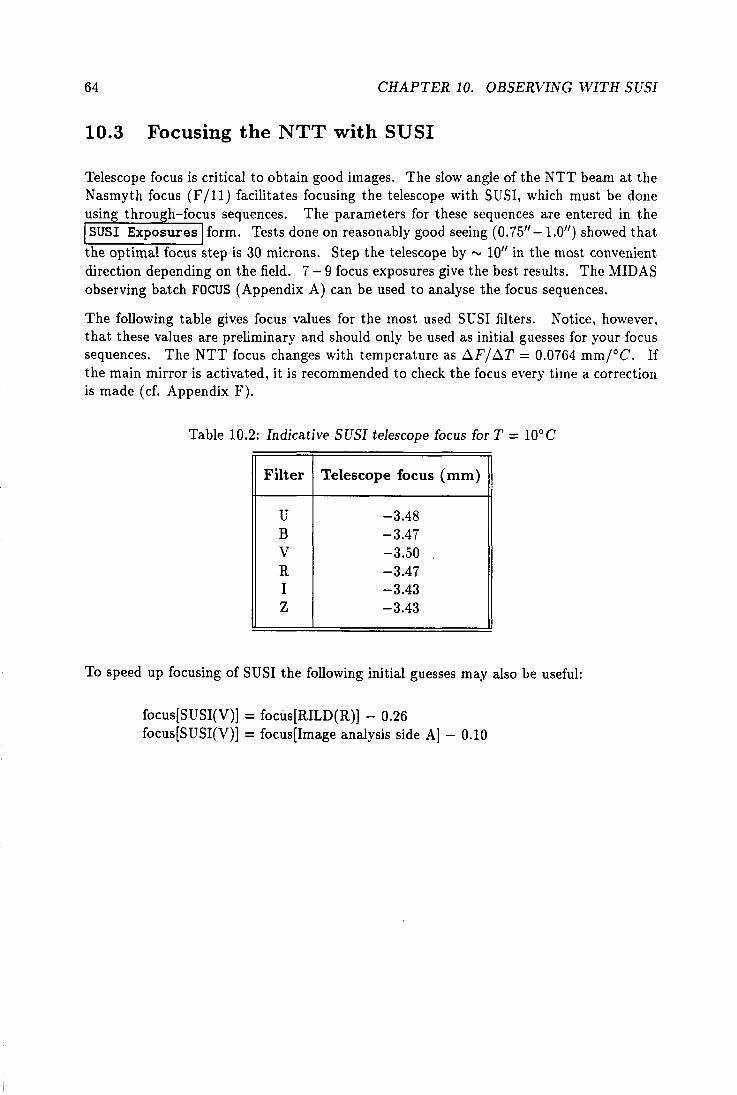
64 CHAPTER 10. OBSERVING WITH SUSI
10.3 Focusing the NTT with SUSI
Telescope focus is critical to obtain good images. The slow angle of the NTT beam at the Nasmyth focus (F /11) facilitates focusing the telescope with SUSI, which must be done using through-focus sequences. The parameters for these sequences are entered in the I SUSI Exposures I form. Tests done on reasonably good seeing (0.75" -1.0") showed that the optimal focus step is 30 microns. Step the telescope by '" 10" in the most convenient direction depending on the field. 7 - 9 focus exposures give the best results. The MIDAS observing batch FOCUS (Appendix A) can be used to analyse the focus sequences.
The following table gives focus values for the most used SUSI filters. Notice, however, that these values are preliminary and should only be used as initial guesses for your focus sequences. The NTT focus changes with temperature as !::.F /!::.T = 0.0764 mm;oC. If the main mirror is activated, it is recommended to check the focus every time a correction is made (cf. Appendix F).
Table 10.2: Indicative SUSI telescope focus for T :::: lOoC
Filter Telescope focus (mm)
U -3.48 B -3.47 V -3.50 R -3.47 I -3.43 Z -3.43
To speed up focusing of SUSI the following initial guesses may also be useful:
focus[SUSI(V)] = focus[RILD(R)] - 0.26 focus[SUSI(V)] = focus[Image analysis side A] - 0.10

Chapter 11
Additional Information about EMMI
11.1 G hosts and image anomalies
11.1.1 Imaging (RILD and BIMG)
Most ghosts in imaging are due to a reflection between the CCD and a lens surface, and as such, they depend on the reflectivity of t~e CCD surface and the efficiency of the antireflection coatings. The antireflection coatings on EMMI have a low reflectivity (1% in the red and 0.4% in the blue, compared to 2% for EFOSC). A sky concentration already familiar from EFOSC is also present in EMMI. This type of effect is very difficult to avoid in any focal reducer design. It is due to light - from the sky background and from stars - that is reflected back into the camera by the CCD and returned by some optical surfaces. The effect is not very noticeable in normal flatfield exposures. ,
An on-axis star has a faint halo around it with an intensity level dropping to 10-4 at 5 pixels from the parent star (RILD). This was measured without any filter in the beam.
In RILD, filters are tilted so reflections between the CCD surface and the filter are excluded. However, multiple reflections inside the filter may in principle lead to satellite images close to the parent if the filter has a small wedge. No such ghosts with a level greater than 10-3 were found for filters 587 to 645. In BIMG, filters are in the converging beam and no nearby in-focus ghosts are expected.
11.1.2 Spectroscopy (RILD, REMD and BLMD)
Image ghosts and anomalies may originate from both the grating (or grism) and the spectrograph optics.
Grating ghosts are caused by periodic variations in the position of the grooves. Longperiodic errors of the grating engine produce line satellite (Rowland) ghosts which perturb the line shape and so may change the width and shape of the point spread function. The
65

66 CHAPTER 11. ADDITIONAL INFORMATION ABOUT EMMI
observer should be very careful in looking for faint or unidentified lines, especially when observing objects with strong emission lines, because these might be the more dangerous Lyman ghosts. These are far away from the parent line and are caused by short-periodic errors of the ruling engine. According to manufacturers' specifications, all EMMI gratings have Lyman ghosts < 10-4 except No.6 (3.8 x 10⁻⁴ ), No.7 (1.8 x 10⁻¹ ) and No.9 (17 x 10-4 ).
The efficiency curves of some gratings show irregularities called Wood's anomalies. These anomalies depend strongly on the polarization of the incident light and are most prominent when the polarization is perpendicular to the grooves. Wood's anomalies affect gratings numbers 3, 7,8 and 11.
The curved cemented surface inside one of the doublets of the red collimator happens to be exactly perpendicular to the incoming diverging beam. It is effectively behaving like a plane parallel glass plate in front of the grating (however with a very low reflectivity of about 4 X 10⁻⁴ ). The white light ghost image of the slit generated by this surface was moved outside the CCD field by applying a small tilt to the collimator. A complementary ghost is formed by light that is dispersed by the grating, reflected by the cemented surface and dispersed a second time. This appears on the CCD as ghosts of a few times 10-4 of bright emission lines that are in the right-hand half of the CCD image, located approximately twice as far from the right-hand edge of the CCD as their parents. So far we only noticed ghosts in calibration echelle spectra, where some of the bright Ar lines of the ThAr calibration lamp produce ghosts of this type.
Interorder stray light was measured with grism #3 as cross-disperser and the red flatfield lamp. The absolute level is highest near 700 nm and reached 1.9% of the continuum with echelle grating #9. With #10 the stray light level was 6% of the continuum at 750 nm. On request, a stray light mask can be mounted in the intermediate focal plane (between the collimator and the focal reducer). This reduces the stray light level to 1.2% and 3 %, respectively.
A stray light gradient which does not depend on the continuum intensity is present when combining echelle grating #10 with grism #3 as cross-disperser. The stray light is strongest near the top of the CCD with a level of about 50 e- in a 1 hour exposure. The effect was only observed with grism #3 and was not noticed with grism #4 as crossdisperser. The stray light seems to be generated inside the transfer collimator and its cause will be further investigated. A 50 pixels wide vertical band of scattered light occurs about 200 pixels from the right edge of ecchelle-format spectra taken with grating # 10. It has only been noticed in dome flat field spectra and probably results from straylight entering from the N athmyth apaerture and being dispersed by the grism. The feature could not be detected in well exposed standard star or comparison spectra.
The blue mirror train shows a 10% reflectivity dip with a width of about 5 nm in one polarization at around 370 nm, which could easily be mistaken for an absorption feature. The antireflection coatings of the red lenses also show some dips that are however not polarization-dependent and several 10 nm wide.
The dichroic prism shows large variations in the efficiency in the polarization perpendicular to the slit up to 30%. The region between 400 and 480 nm is heavily polarized and it is not recommended to use the dichroic prism on polarized objects.
11.2. IMAGE QUALITY, SCALE AND DISTORTION 67
11.2 Image quality, scale and distortion
11.2.1 Imaging
The measured scales determined using stars in an astrometric field are 0.268 ± 0.004 arcsec/pix in the red, and 0.37 ± 0.005 arcsec/pix in the blue.
The above coefficients are but the first terms in the polynomial that describes the transformation from sky to pixel coordinates. Higher order terms must take into account lateral colour (chromatic variation of focal length) which goes with the first power of the radial distance, and 3rd and 5th order distortions.
Spot diagrams in RILD and BIMG cameras are given in Figures 11.1 and 11.2. These were calculated assuming a perfect telescope and atmosphere. In RILD the image quality (80% energy concentration) is better than 10jlm in most of the field and better than 20jlm out to the corners. In BIMG the image quality is better than 20jlm in most of the field.
At wavelengths beyond 950 nm, the PSF develops wings which are attributed to light diffusion inside the CCD.
The spot diagrams show that optical aberrations and lateral colour produce image elongations in the field that cannot be neglected. Note that the elongation axis direction varies with field position. Other possible factors contributing to image elongation are: sampling effects in the CCD, filter image quality, "bubbles" of air accumulating over the M 1 when the dome is not well ventilated, atmospheric dispersion and telescope tracking including wind buffeting effects and field rotation. Most of these produce an elongation that is constant in the field. Image size differences of 0.1" in X and Y on I" images are normal and do not necessarily point to telescope tracking errors.
11.2.2 Spectroscopy
The image scales given for imaging also apply to EMMI used in spectroscopy. High-angle grisms and gratings produce anamorphosis which results in a slit image that is narrowed (the usual case) or widened by a certain factor. The scale along the slit is not affected. At the CCD centre, the anamorphic factor A is equal to:
cos(8 + ~) A - -----:,-=--- cos( 8 - ~ + 7P) ,
where </> is the angle between incident and diffracted beams at the field centre, 8 the grating angle and 7P the field angle. For gratings we have:
0= arcsin(n x m x >.) , 2 X 10⁻⁷ X cos £ 2
where n is the number of grooves/mm, m the order, >. the wavelength in nm. </> = 5.50
in EMMI while 1/.' = arctan 120~F#' where x is the distance in the CCD focal plane from the field centre in mm and F# is the camera speed.

68 CHAPTER 11. ADDITIONAL INFORMATION ABOUT EMMI
WAVELENGTH
O.4200"m o.4860"m o.5876"m o.6563"m Q9~90"m
.. . . " I {i;' ~. • • -~ -. --·-1
37.3mm ;: ,,/
'(
• j
-+-5.s' -~ 29.8mm
w U Z ~
-~ I
4J--U) 4.2' -~ -Q
~ i I >< c( ~ ~
0
-*- + '0
2~~ 4- 4>-14.9mm .0 00 -
i
4- I d-+ -$-- -.@ .. -* Omm 00 o •
,
Figure 11.1: Spot diagram showing theoretical image quality in RlLD with the F/5.2 cam-era, at a single focus setting at various wavelengths and radial field points.
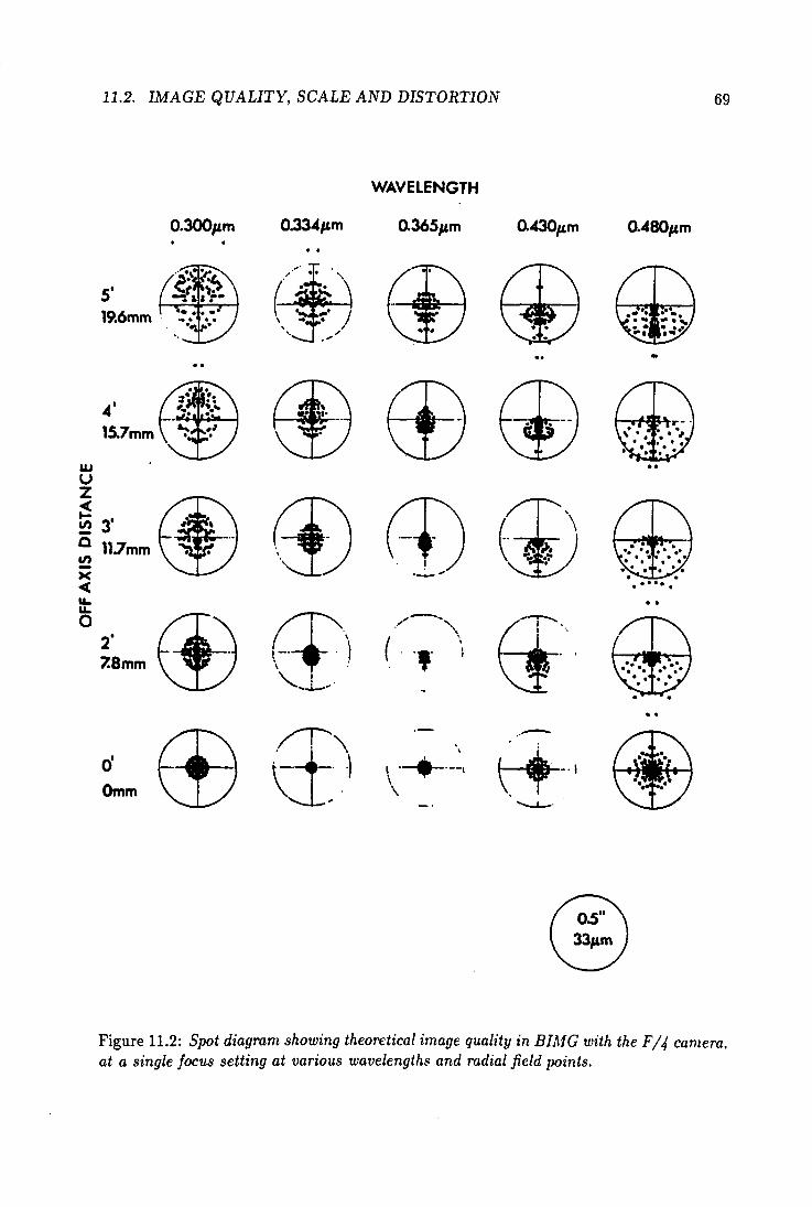
11.2. IMAGE QUALITY, SCALE AND DISTORTION
w U
5' 19.6mm .
4' 15.7mm
~@ !a 3' .., ~ 11.7mm - ~ . ..
<II( ~ ~ o
2· 7.8mm
0' Omm
WAVELENGTH
(
\
\'+'--1 \ \
.. -t+-I . .
{o;'\ ~
69
••
..
••
Figure 11.2: Spot diagram showing theoretical image quality in BIMG with the F /4 camera. at a single focus setting at various wavelengths and radial field points.

70 CHAPTER 11. ADDITIONAL INFORMATION ABOUT EMMI
Gratings #9 and #10 have () = 28.7° and 63.5°; the anamorphism is 0.96 and 0.82, respectively.
Grisms have A = 1 at the central wavelength, A > 1 towards the red and A < 1 towards the blue. Here we have:
• () = 40° for grism #6 and 26° for grism #5 (less for other grisms)
• <t> = 0°
• 'IjJ = arctan (50':F¥)' where x is the distance from the field centre in mm.
In the case of grism #6, A = 0.94 at the red end of the spectrum and A = 1.07 in the blue. Grism #5 has less anamorphosis with A = 0.97 and 1.04, respectively. The anamorphosis for other grisms is less.
If grisms are used as cross-dispersers in echelle spectroscopy, the scale in the slit direction will be affected: in the case of grism #6 for instance, the height of the spectrum is 14% smaller in the red orders than in the blue.
With high-angle grisms and gratings, long slit spectra will show spectral line curvature. Spectral lines have a parabolic shape with shifts towards the blue at the upper and lower edges of the slit of up to several pixels depending on the grating used and the wavelength settings. The long-slit spectral reduction package LONG in MIDAS automatically corrects this distortion.
11.3 Filter properties
All filters are permanently mounted in their cells. Although it is possible to use blue filters in the red and vice versa (for example in the overlap region; 400 to 500 nm), filters should normally be used on the wheel they are intended for. Blue filters are mounted at o degrees in their cells while red filters are at 5 degrees to avoid reflections between the CCD and the filter. Below slit filters are glued in a rectangular cell that only permits to use them on one of the two below slit wheels of EMMI.
As a general rule, all filters are blocked to better than 10-4 to 1.2J.lm. Note that the optices of the blue arm of EMMI provides some additional blocking to red light: 10% beyond 600 nm and less than 2% between 800 nm and 1.2J.lm.
The spectral properties of colour filters are to a great extent independent of the angle of incidence, </>, and can be assumed to be constant within the field, both in blue and red imaging. The central wavelength of interference filters shifts to the blue if this angle deviates from 0 degrees. The following formula applies:
where </> is the angle of incidence and n the effective refractive index of the material forming the spacer cavity. The EMMI blue filters are placed in the diverging F /11 beam in front

11.4. IMAGE STABILITY AND FLEXURE 71
of the blue camera, so the effective filter curve (averaged and weighted for all incidence angles in the F /11 cone) will be somewhat broadened and blue-shifted compared to the filter curves measured at 0 degrees incidence. The effects are likely to be on the order of only a fraction of nm in the blue and may be neglected with the bandpasses used in the current set (> 5 nm FWHM) of filters.
The EMMI red filters are placed in the parallel beam between the collimator and the camera. The angle of the beam with the optical axis depends on the field position of the object. However, red filters must be tilted 5 degrees in order to avoid reflections between the filter and the CCD, and so the angle of incidence varies from 0.5 degrees to 9.5 degrees. The effect on the bandpass of filter #601 has been measured at incidence angles between 0 and 15 degrees, and a value of n = 2.06 has been found. The wavelength shift is significant: about 0.3% of the central wavelength (30% of the FWHM: 2.2 nm) at 9.5 degrees in the case of #601.
Observations are affected in two ways. First, observers should remember that filter central wavelengths, and to a lesser extent also FWHMs, are field-dependent and take account of this, for instance by positioning critical objects nearer to the lower edge of the chip. Secondly, bright sky emission lines that are not in the filter passband at edge of the field may be just in at the other edge, giving rise to a background slope which then requires additional attention in flatfielding.
U and B photometry should normally be done in the blue arm of EMMI. The Bb (blue B) filter is a B filter intended for use in the red arm of EMMI, and is open towards the UV in order to approximate the regular B as well as possible. The red optics of EMMI have a sharp cut-on at 390 nm due to the coatings, and so the effective central wavelength/bandpass of the Bb filter is 429.5/79 nm as opposed to 423/94 nm for the B filter used in the blue arm of EMMI. We expect that better results (efficiency and colour transformation coefficients) will be obtained with the B filter, but no systematic study has been made so far. .
Since the blue and below slit filters are used in diverging beams, they affect the focus. The red filters are used in parallel beam and introduce less important defocus. The below slit filters are normally used with a wide slit for flux calibration on standards, where it is not important to achieve the optimum spectral resolution, so no focus correction is necessary.
The image quality of some filters was investigated by imaging a 200J,Lm (1.07") pinhole in a starplate. There is some evidence of image degradation by filters #588 and #606. Some improvement may be expected by refocusing, as the focus was set at the optimum found for the Band R filters. No nearby ghosts could be identified down to a level of 10-3 .
11.4 Image stability and flexure
EMMI rotates with the adapter to follow field rotation. Depending on the duration of the exposure and the location of the object, instrument rotations of 180 degrees and more may result. The instantaneous angle is displayed by the instrument control program.
Instrument flexure has been measured in RILD, REMD and BLMD. The position of the
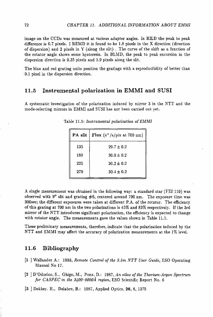
72 CHAPTER 11. ADDITIONAL INFORMATION ABOUT EMMI
image on the CCDs was measured at various adapter angles. In RILD the peak to peak difference is 0.7 pixels. I REMD it is found to be 1.8 pixels in the X direction (direction of dispersion) and 2 pixels in Y (along the slit) . The curve of the shift as a function of the rotator angle shows some hysteresis. In BLMD, the peak to peak excursion in the dispersion direction is 0.35 pixels and 1.9 pixels along the slit.
The blue and red grating units position the gratings with a reproducibility of better than . 0.1 pixel in the dispersion direction.
11.5 Instrumental polarization in EMMI and SUSI
A systematic investigation of the polarization induced by mirror 3 in the NTT and the mode-selecting mirrors in EMMI and SUSI has not been carried out yet.
Table 11.1: Instrumental polarization of EMMI
PA slit Flux (e-/s/pix at 700 nm)
135 29.7 ± 0.2
180 30.0 ± 0.2
225 30.2 ± 0.2
270 30.4 ± 0.2
A single measurement was obtained in the following way: a standard star (FEI 110) was observed with 9" slit and grating #6, centered around 700 nm. The exposure time was 300secj the different exposures were taken at different P.A. of the rotator. The efficiency of this grating at 700 nm in the two polarizations is 45% and 83% respectively. If the 3rd mirror of the NTT introduces significant polarization, the efficiency is expected to change with rotator angle. The measurements gave the values shown in Table 11.1.
These preliminary measurements, therefore, indicate that the polarization induced by the NTT and EMMI may affect the accuracy of polarization measurements at the 1 % level.
11.6 Bibliography
[1 ] Wallander A.: 1993, Remote Control of the 3.5m NTT User Guide, ESO Operating Manual No 17.
[2 ] D'Odorico, S., Ghigo, M., Ponz, D.: 1987, An atlas of the Thorium-Argon Spectrum for CASPEC in the 3400-900oA region, ESO Scientific Report No.6
[3 ] Dekker. H., Delabre, B.: 198;, Applied Optics, 26,8, 1375

11.6. BIBLIOGRAPHY
[4 1 Dekker, H., Delabre, B., D'Odorico, S.: 1986, SPIE, 627, 339
[5 1 Gilliotte, A.: 1992, Image Quality Filters Catalogue, Internal ESO publication
[6 J Melnick, J., Dekker, H., D'Odorico, S.: 1989, ESO Operating Manual #4
[7 1 Prieur, J.-L., Rupprecht, G.: 1990, Efficiencies of EMMI, ESO internal report
73
[8 1 Wilson, R. N., Franza F., Noethe L., Andreoni G.: 1991, Journal of Modern Optics, 38,219.
Appendix A
EMMI Observing Batches
There are several batch programs (procedures) in MIDAS that are needed for observing with EMMI. The images from the two EMMI CCDs and from SUSI are automatically transfered to the MIDAS workstation.
To log-on to the Unix/MIDAS workstation enter username CCD and password lasilla.
The MIDAS implementation at the NTT uses two monitors, of which one is exclusively dedicated to image display. After log-on a number of XII windows appear on the lefthand screen. The light blue window at the upper right is the data transfer log window. windows. MIDAS is automatically started in the white window. Images arrive from the EMMI and SUSI CCDs in FITS format (.mt) and are automatically converted to .bdf format and displayed in the large display window (right monitor). Approximately I Gby of disk storage is available for MIDAS. A small Graphical User Interface appears on top of the display window and provides convenient access to the MIDAS observing batches. These can be executed by positioning the mouse cursor in the corresponding field, and clicking the left button. Some of these fields are pulldown menus offering several options. For example, if you click I Focus I you get two options: 1 sequence I and IW;tdge I, for measuring focus sequences and exposures with the focus we ge respectIvely. you select the I sequence I option, a pop-up window will appear where you will be requested to give the parameters of the focus sequence (start, step). Other batches (e.g. POINT) also prompt in the same way for pointing parameters. The blue key provides some utilities. The use of this graphical interface is straightforward.
Internally, the graphical interface works by simply composing the corresponding MIDAS commands and sending them to the MIDAS window. Therefore, it is also possible to give the commands by typing them in that window. The MIDAS observing procedures are briefly described below.
A.l MIDAS procedures
The MIDAS observing batches may be run by clicking the corresponding field on the graphical XII user interface that appears on top of the MIDAS display window.
74
A.2. MAKING MOS PLATES 75
~~ loadn image [-n ] Load image after calculating cuts. The optional parameter (n) is the scaling factor as in the MIDAS command load.
focus: This is a pull-down menu with 2 options: focus wedge Focus using focus wedge; RILD mode only and
Focus using through-focus sequences L-.-____ ---'
1 seeing I: (~~ seeing) .Deter~ine se~ing. In MIDAS the procedure automatically determines the approprIate pIxel scali ng, and therefore the same procedure can be used for the three image types (RILD, BIMG and SUSI).
1 poin~ \: (~~ point [xsli t] [ysli t] [angle] [flag]) . Point offsetting from direct Images. The procedure prompts for the parameters if not given. The angle is defaul ted to o. If the flag is set to C the cursor is used to define the position instead of Gaus sian fits (default).
/ rotate/: (~~ rotate). Determine angle between two objects. This is a pull-down menu with two options for / g~u~s /' and I cursor I centreing of the objects. Notice th at rotate assumes that the s t IS oriented NS.
I trace \: This calls the MIDAS command extract/trace. The trace is extracted between a fiducial point and the position of the mouse cursor. Use the arrows to change the fiducial mark. The keyboard keys 1-9 may be used to speed up this motion.
1 catal;5J: This pull-down menu has options to list the headers of the RED, BLUE, and I files in the MIDAS window, and to reset the catalogues. Once the catalogues
are reset, they must be created again with the create/icat command. This is automatically done at the beginning of the session.
I utils I: This pull-down menu contains options to get the cursor and to print the graphics windows on the laser printer.
These batches are described in more details in the Remote Control User Guide of the NTT (ref [1]).
A.2 Making MOS plates
The MIDAS context EMOS allows to prepare interactively the ASCII tables used by EMMI to punch MOS aperture plates. EMOS uses a mouse driven Xll graphical interface and can be run at any MIDAS installation equipped with Xl1. This interface consists of three elements: a parameter window, a dialog window, and a set of buttons and pulldown menus. These buttons are "pushed" by clicking the left mouse button at the corresponding position. EMOS has an on-line help facility which works by clicking the
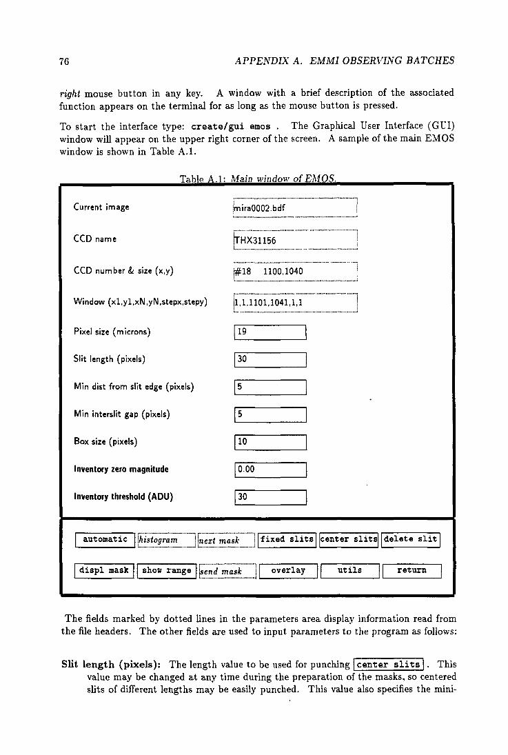
76 APPENDIX A. EMMIOBSERVING BATCHES
right mouse button in any key. A window with a brief description of the associated function appears on the terminal for as long as the mouse button is pressed.
To start the interface type: create/gui emos. The Graphical User Interface (GUI) window will appear on the upper right corner of the screen. A sample of the main EMOS window is shown in Table A.I.
Table A.I: Main window of EMOS.
Current image ; ............................................................ _··· .. ··· .. ··· .. ···· .. ··· .. ··· .. ·1
r. .. i.~.~_~.~.~~.:.~.~.:. .... _ .. _ ... _ .... _ ... _ ... _ ... _ ......... _ ... ...J ~ ............................................................... -....... -................. ~
CCD name ~.~~.~.~ .. ~.~~ .. -...................... -... _ ... -... _ .... _ ........ _ .. CCD number &. size (x,y) j#18 1100.1040
.................................................................................................
~ ....... -... -................... -... -......... -... -..................................... ~ Window (xl ,y1 ,xN ,yN ,stepx,stepy) :1.1.1101,1041,1,1 :
L .................... _ ................................................................... _j
Pixel size (m icrons)
Slit length (pixels) po Min dist from slit edge (pixels)
Min interslit gap (pixels)
Box size (pixels)
Inventory zero magnitude 10.00
Inventory threshold (ADU)
I automatic I ~:~~~~~?:~:~::~:::~:::J ~:i~~:::~~:i~~:::~::::J I fixed slits Ilcenter slitsll delete slit I
I displ mask II sho~ range I ~~:~~~:~:~~~::~:::J I overlay II utils II return
The fields marked by dotted lines in the parameters area display information read from the file headers. The other fields are used to input parameters to the program as follows:
Slit length (pixels): The length value to be used for punching 1 center slits I. This value may be changed at any time during the preparation of the masks, so centered slits of different lengths may be easily punched. This value also specifies the mini-

A.2. MAKING MOS PLATES 77
mum slit length for the I automatic I mode. The shortest slit that can be punched is 8.6 arcseconds.
Min dist from edge (pixels): Specifies the minimum distance allowed for an object to lie from the end of its own slit. This parameter is necessary because in the I automatic I mode EMOS optimizes the lengths and centering of the slits to fit the maximum number of objects in one mask without overlapping slits.
Min inters lit gap (pixels): Sets the minimum separation allowed between neighbouring slits.
Box size (pixels): Size of the square box used for centering objects (MIDAS command center/gauss ).
Inventory zero magnitude: Zero point of the magnitude scale (for 1 sec integration). This value is used in the automatic search mode for selecting the magnitude range of the galaxies to be chosen. If the zero point is not given, the programme uses instrumental magnitudes as determined by the MIDAS package INVENTORY.
Inventory threshold (ADU): Defines the threshold used by INVENTORY for automatically finding objects (used only in the I automatic I mode).
To change any of these parameters, simply move the cursor to the corresponding field and type the new value. It will be sent to MIDAS as soon as the cursor is moved out of the field. Check in the MIDAS session window that this happens.
The main EMOS menu has three options: I load I to load an image and read the descriptors, I MOS I that leads to another menu for preparing the mask, and I Utils I which is a pulldown menu containing a number of MIDAS utilities commands (e.g. createl display. create/ graphics, etc.). After you click I load I the list of MIDAS . bdf files in your working directory appears in a pop-up window. Click the name of the file you wish to load. Then go to I MOS I. A new set of buttons appears in the GUI with the configuration shown in Table A.I.
I automatic 1 This pull-down menu has two options: I stars I and I ~alaxies I. EMOS prompts for a sub-image, which must be specified giving the lower-left an upper-right corners with the graphics cursor, and calls INVENTORY to search in the sub-image for objects brighter than the threshold value defined in the parameters field. INVENTORY determines the centroid and the magnitude of each object, and does a star/galaxy separation, plotting a yellow circle on top of all the stars or galaxies found. The histogram of magnitudes is displayed and, using the cursor, you must specify the magnitude range of the objects (stars or galaxies) to be used for the mask. The button histogram is enabled and may be used to change the magnitude range later if required. ta e WIt all the objects selected by INVENTORY within the given magnitude range is prepared, and all objects within the specified magnitude range are plotted in red. Then a sub-set is selected such that

78 APPENDIX A. EMMI OBSERVING BATCHES
the number of objects that fit in one mask is maximized by choosing slits-lengths as close as possible to the minimum value specified in the parameters window. The command I next mask I can be used to iterate until all the objects in the table have been selected (see below).
histogram A plot of the distribution of magnitudes of the objects found by INVENIS gIven, and the graphics cursor is used to select the magnitude range of the objects
to be included in the list to be punched.
next mask This command allows to punch the next objects in the list prepared in the automatic mode. By using this command repeatedly, all the objects within the selected
magnitude range may be punched systematically in several masks.
I fixed slits I This command allows slits of any length to be defined interactively. Mark the lower and upper position of the slit with the graphics cursor using the left button of the mouse. The first time the X position of the slit and the lower Y edge are defined. Click again to define the upper Y edge of the slit. The X position of the cursor is ignored the second time.
I centered slits I Center the box on an object and click the left mouse button. The X,Y position of the slit is defined by a Gaussian fit (center/gauss). The length of the slits is defined in the parameter definition window as described above. I centered slits 1
and I fixed slits I may be used both to create a new mask or to modify an existing one.
I delete slit I. Click at the position of a slit (within 15 pixels) to delete it.
displ mask This pull-down menu allows to plot the current mask top of the displayed
image ( show current mask ), to load a different mask from the disk (I load new mask j), or to erase the current mask to start a new one (I reset mask I). In order to avoid erasing the current mask accidentally, the last two options request confirmation. The overlay pull-down menu may be used to choose the colour in which the masks will be dISP aye .
show range This command is used in 2 steps: the first time on the list of the 6 EMMI gnsms WIt t e maximum possible wavelength range appears on the MIDAS window, and a new parameters window appears in the GUI. You must enter the grism number, and the required wavelength range. I show range I is then used again to delineate the area where the specified range may be realized and to show the region which can be reached mechanically by the punching engine. Remember that using grisms the wavelength range depends on the position of the slit.
I send mask I After the mask has been prepared, this command sends the final ASCII table to the NTI computer to be used by EMMI. The name of the file is given. It is composed of the name of the direct image used to prepare the mask plus a number. This command also allows to store the current mask on disk. The same name is used.
I overlay I Allows selecting the colour of the line graphics on the image display. This

A.2. MAKING MOS PLATES 79
command is particularly useful to modify masks. An option to clear the overlay plane is also provided in this menu.
I utils I This pulldown menu contains a number of useful utilities.
I return I Return to main menu.
Appendix B
EMMI Efficiencies
The efficiencies of the individual EMMI optical components are given below. These include the transmission of EMMI optics, the absolute reflectivities of gratings used in the blue and the red arms, the transmission curves of grisms, the quantum efficiencies of the CCDs presently mounted. The efficiency of EMMI optics in the DIMD mode is shown in Figure 2.3.
80
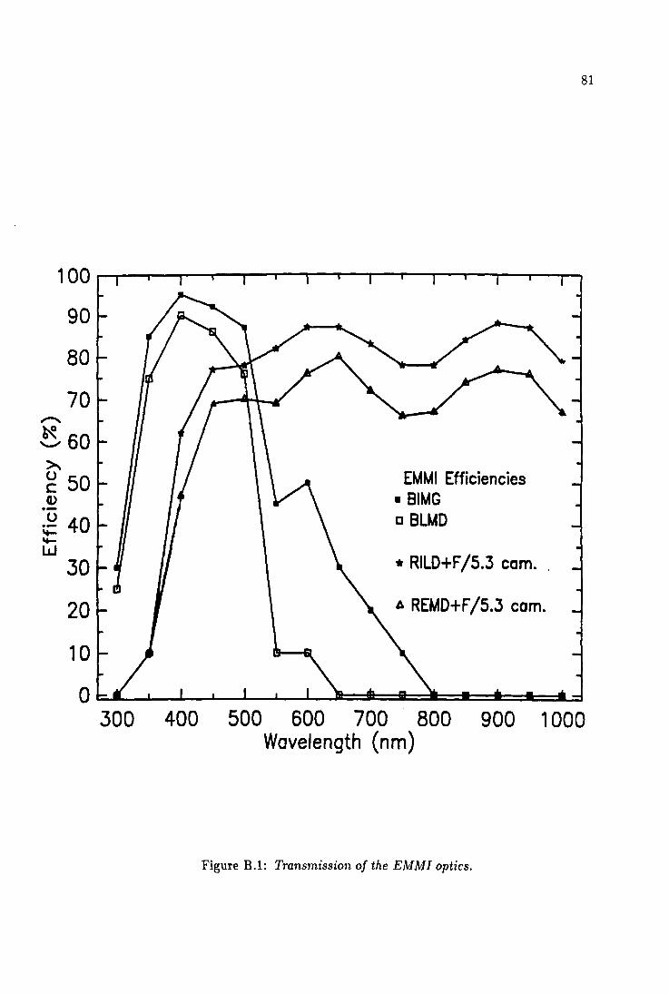
81
100--------~~~~--r-~~~~--~~~
~
90
80
70
~60 ~ g 50 Q) .-~ 40 't-W
30
20
10
EMMI Efficiencies • BIMG D BlMO
* RllO+F /5.3 com.
A REMD+F /5.3 com.
O~~~---~L-~~~~~~~~~~~
300 400 500 600 700 800 Wavelength (nm)
Figure B.1: Transmission of the EMMloptics.
900 1000
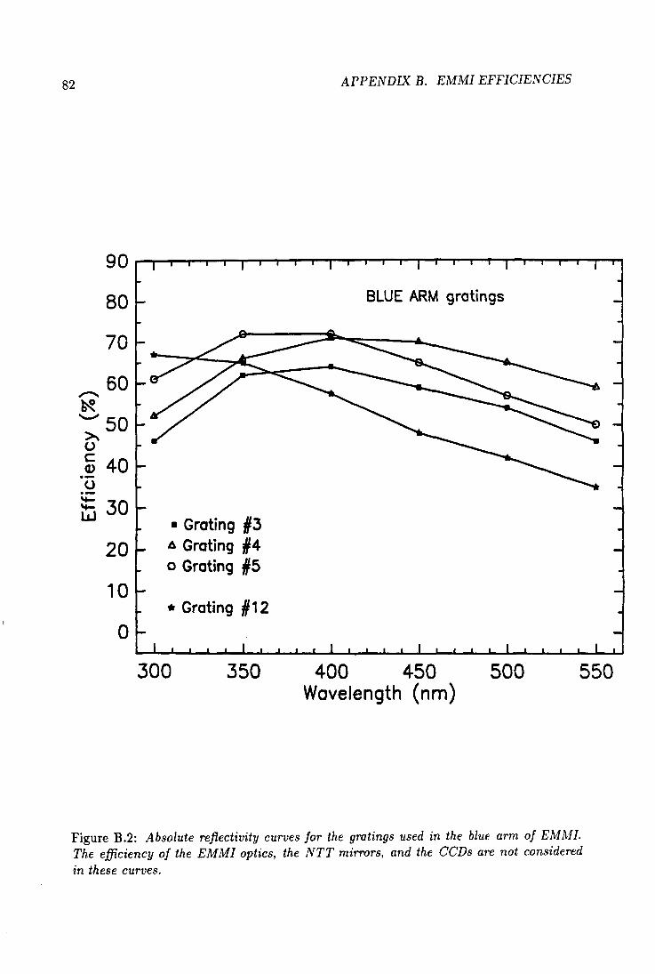
82 APPENDIX B. EMMI EFFICIENCIES
BLUE ARM gratings
300 350 400 450 500 550 Wavelength (nm)
Figure B.2: Absolute reflectivity curves for the gratings used in the blue arm of EMMI. The efficiency of the EMMloptics, the NTT mirrors, and the CCDs are not considered in these curves.

83
90
80 RED ARM gratings
70
60 r-.. ~ ........ 50 ~ () c: Q)
() .-"4-'+-W
40
30
20
10
a 400
A Grating #6 o Grating #7 • Grating N 13
500 600 700 800 Wavelength (nm)
900 1000
Figure B.3: Absolute reflectivity curves for the gratings used in the red arm of EMMI. The efficiency of the EMMI optics, the NTT mirrors, and the eeDs are not considered in these curves.
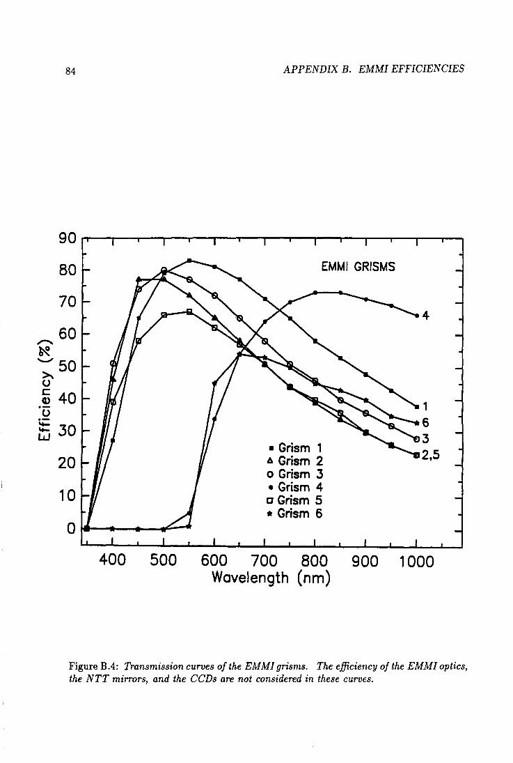
84 APPENDIX B. EMMI EFFICIENCIES
90
80 EMMI GRISMS
70 4
60 '" ~ '-' 50 ~ 0 c Cl) .-0 .-
'to-'to-W
40 1 S 30 3
• Grism 1 2,5 20 6 Grism 2 o Grism 3
10 • Grism 4 a Grism 5 * Grism 6
0
400 500 600 700 800 900 1000 Wavelength (nm)
Figure B.4: Transmission curves of the EMMI grisms. The efficiency of the EMMloptics, the NTT mirrors, and the CCDs are not considered in these curves.

Appendix C
He-Ar calibrations for EMMI Grisms
Representative He-Ar spectra taken with the EMMI grisms are presented below. All spectra were obtained using a I" slit, fast readout mode, and the exposures times given in Table 5.3 and were averaged over 45 lines. Some prominent lines are identified. The full He-Ar lines tables are available in MIDAS.
I
f-
f-
~
f- J'
I
0.0
I
ORIS .. No 1
HeAr
J
I
500.0
1/)1'0 ~~ -I/)
r.: " ~8 ::~ 1)1'0
I .I I
1000.0 Position
I I I) 01) ....
:l~ (Ii -~ ;S
-.
-
-
II - -I I
1500.0 2000.0
Figure C.l: He-Ar line identifications for grisms #1
85

86
I
r
f-
I-
I-
f-I
0.0
APPENDIX C. HE-AR CALIBRATIONS FOR EMMI GRISMS
, ~ ,..: ..,. ..,.
GRISM No 2
HeAr
I I
500.0
r-~ Q I/)
J
I'
...L
1000.0 Position
~ ,..: U) U)
, , C\I Q U)CII I/)
~ ..,.r-
uS eli uS -0 ~:s r-
-·
-
· -
· lJ........~
...L I
1500.0 2000.0
Figure C.2: He-Ar line identifications for grisms #2 and #3.

I
~
I-
I-
~
I-
f-
l-I
0.0
0.0
I II) I/)
~ I/)
GRISt.( No 4
HeAr
I
500.0
I/) ... r-: ... ...
~ r-: II) II)
GRISt.( No 5
HeAr
500.0
I
1000.0 Posilion
1000.0 Posilion
II) ... CIi ~
I
I
CI CO)
CIi ... CII
I
1500.0
... i
1500.0
, II) to-.,; -II) CII
-·
-·
· · -
·
I '-I
2000.0
2000.0
Figure C.3: He-Ar line identifications for grisms #4 and #5.
87

Appendix D
Ar Calibrations for EMMI Gratings
Spectra of the Ar lamp taken with two EMMI gratings (#6 and #7) centered at the blaze wavelength are given below. Line identification for other grating angles can easily be made using the plots given in reference [1].
GRATING No 6
Ar
0.0 500.0 1000.0 Position
1500.0 2000.0
Figure D.1: Ar line identifications for Grating #6 centred at blaze position
88

0.0
GRATING No 7
Ar
500.0
.... N M o CO
1000.0 Position
1500.0
Figure D.2: Ar line identifications for Grating #7 centred at blaze position
89
2000.0

,Appendix E
Th-Ar Atlas for High Disperion Gratings
Spectra of the Th-Ar lamp taken with the EMMI echelle grating #10 are similar to those of CASPEC. We give here a chart with the approximate central wa.velength of some orders for the EMMI echelle grating #9 and grism #3 used a cross-disperser.
90

91
Figure E.1: Th-AR Atlas for echelle grating #9 and grism #3 as cross-disperser

Appendix F
The NTT Active Optics System
F.l Image analysis
A dichroic beam splitter has been installed that allows the image analysis system and the autoguider to work in parallel. Nevertheless the active optics software is not yet able to perform automatically parallel image analysis. A manual operation of the parallel mode is possible when the guide star is bright enough. At the end of the exposure, a correction can be applied (new M 1 and M 2 setting) at the request of the astronomer. This correction takes about two minutes and the telescope cannot be moved in the meantime.
The relevant parameters in the present context are the rms and d80 The meaning of these parameters is as follows:
rms This is the r.m.s. error in arcsec of the residual high spatial frequency errors. If the rms is large, the solutions are largely determined by atmospheric and dome seeing and therefore it is not recommended to reset the mirrors. Under very good seeing conditions the rms is below 0.12, while for very bad conditions the rms can be higher than 0.20. The recommended limit is 0.18 beyond which no corrections should be applied to the optics.
d80 This is the diameter within which 80% of the light is concentrated and is thus a direct measure of the optical quality of the telescope. The various components that contribute (quadratically) to d80 are shown. The principal terms are spherical aberration (spher), coma, astigmatism (ast), triangular coma (tri), and quadratic coma (quad). Defocussing is given but is not considered in the total sum. On nights of exellent seeing, the optical quality may be adjusted to d80 < 0.1", but twice this value is still aceptable.
Remember! Applying corrections when the rms is high may degrade the optical quality of the telescope instead of improving it!.
There is a small offset between the telescope focus at the image analysis camera, and the focus at EMMI or SUS!. This offset has not yet been accurately measured, and therefore it is advisable to check the focus every time the optics are reset using the AOS.
92

Appendix G
Checking the EMMI focus yourself
The EMMI focus is usually determined by the operations staff but, should you want to check the relations given, the following procedures may be followed. Use one of the internal lamps. Typically exposures of a few seconds with He or Ar are sufficient.
RILD: do a through-focus exposure using the test starplate which has holes of f'V 200llm diameter through the R filter and run FOCUS (MIDAS). This pinhole is not permanently mounted; include it in your setup request. Remember to select exposure type foi and to fill the I RILD Focus param., form. You may also take an exposure with the focus wedge to test its adjustment. The focus positions found with the two methods should coincide to within 10 encoder steps.
REMD and BLMD: set the slit to f'V 1" and do a through-focus exposure on the slit with the grating in the zero-th order (A = 0). It is also possible to do a throughfocus exposure on a spectrum; in this case use a spectral lamp and set the grating to the desired wavelength.
Note: echelle gratings #9 and #10 cannot be stepped; here 4 sequential images with different focus settings must be taken. Use the Th-Ar lamp.
93
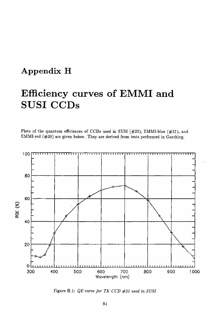
Appendix H
Efficiency curves of EMMI and SUSI CCDs
Plots of the quantum efficiences of eeDs used in SUSI (#2,5), EMMI-blue (#31), and EMMI-red (#36) are given below. They are derived from tests performed in Garching.
100
80~-----+------~------+-----~-------r------+-----~
60~----~------~~~---+-------+------~-------r------~
40~------~~----+-------+-------+-------+---~~~----~
20~----~-------+------~------+-------r-----~--~---'
O~~WU~LU~~~~UU~~~UW~~~~~~~~~~~~~~~
300 400 500 600 700 800 900 1000 Wavelength (nm)
Figure H.l: QE curve for TK CGD #25 used in SUSI
94

TK#31
TK#36
100
80~----~----~~----4------4------+_-----+----~
60L-----~------~------~----_+--~~~------r_----_i
40L---L-~------~------+_------~----~--~---+------~
20~----~----~~----4------4------+_-----+~--~
O~~LU~~LU~~~LU~UL~LU~~LULU~~~~~~~~
300 400 500 600 700 800 900 1000 Wovelength (nm)
100
80~----~----~------4_----_4------+_----_+----~
60~-----+----~~~~--~-----+--~~1-------r------1
40L----4-+------~------~----_+------+_~~~r_----_i
20~~--+-----~-----4------~----1_----_+~~~
400 500 600 700 800 900 1000 Wovelength (nm)
QE curve for TK CCD #31 and TK CCD #36 mounted respectively in the blue arm and the and red arm of EMMI]


![Student Universal Support Ireland [SUSI] : SUSI](https://static.documents.pub/doc/80x56/621e927683ec63593c061b91/student-universal-support-ireland-susi-susi.jpg)


