Employment Growth and Income Inequality: Accounting...

Employment Growth and Income Inequality: Accounting for Spatial and

Sectoral Differences

Valerien O. Pede Department of Agricultural Economics, Purdue University

West Lafayette, IN 47907, USA, [email protected]

Raymond J.G.M. Florax Department of Agricultural Economics, Purdue University

West Lafayette, IN 47907, USA, [email protected] Department of Spatial Economics, VU University

Amsterdam, The Netherlands

Mark D. Partridge Department of Agricultural, Environmental, and Development Economics,

The Ohio State University, Columbus, OH 43210, USA, [email protected]

Selected Paper prepared for presentation at the American Agricultural Economics Association Annual Meeting, Milwaukee, Wisconsin, July 26-28, 2009.

preliminary version

not for quotation – comments invited

Abstract: This paper revisits the inequality-growth relationship accounting for sectoral differences and focusing on US counties. For 8 two-digit industries of the NAICS classification, we estimated a conditional growth model where employment growth depends on regional income inequality and a number of control variables. Spatial econometrics techniques are used to account for spatial dependence. Results indicate that there is no association between employment growth and family income inequality for the Agriculture, Forestry, Fishing and Hunting sector and the Real Estate, Rental and Leasing sector. However, income inequality consistently shows a negative impact on employment growth in the construction sector, and results are mixed for other sectors such as: Manufacturing; Retail Trade; Professional Scientific and Technical Services; Accommodation and Food Services; Educational Services. In several sectors, mixed results were obtained when differentiation is made between urban and rural samples. Keywords: employment growth, inequality, spatial dependence JEL Classification: R0, R11, O15, D30 Copyright 2009 by Pede, Florax and Partridge. All rights reserved. Readers may make verbatim copies of this document for non-commercial purposes by any means, provided that this copyright notice appears on all such copies.

2

1. Introduction

The goal of this research is to investigate the relationship between employment growth and

income inequality, while accounting for sectoral differences at the U.S. county level. There are

several reasons to suspect that a sectorally disaggregated analysis might shed some additional

light on the relationship between income inequality and employment growth. Indeed, the sectoral

composition of regional workforce plays a crucial role in the performance of regional economies

(see Howell and Wolff, 1991; Mangan and Trendle, 2002). In particular, the composition of the

regional workforce in terms of skills types has important implications for its employment

growth.

Commonly in the literature, the effect of workforce composition is captured by indirect

measures such as education attainment or earnings. However, the use of educational attainment

to account for the composition of a labor force may be misleading because of problems such as

variations in the quality of schooling over time and across regions. Earnings are not an accurate

proxy either. For instance, Berg (1970) provided empirical evidence that salaries are not

necessarily closely related to education, and educational attainment of workers may not

necessarily correspond to the skill requirement of their jobs. Some jobs require relatively short

education but are highly paid, while others require several years of schooling but pay less.

It is likely that the effective provision of the workforce composition goes beyond

educational attainment and earnings, and could be captured in terms of regional income

inequality. Indeed, regional economies are characterized by different levels of skill diversity and

this translates into income inequality. Economies dominated by low skills sectors are likely to

have low income inequality because workers are getting paid similar wages. The same applies

for economies dominated by high skill sectors. However, economies that are highly diversified in

terms of type of skills may exhibit high inequality. Changes in the composition of the labor force

will be mostly reflected in terms of income inequality level. Indeed, Howell and Wolff (1991)

empirically show evidence that changes in occupational pattern result in decreasing inequality in

cognitive skills and earnings. Also, Schweitzer (1997) shows that a larger portion of the variation

in earnings is associated with the changing composition of the workforce, rather than with

changing returns to human capital investments. Income inequality and sectoral employment

growth are therefore potentially related through the labor force composition.

3

Apart from income inequality, localization and urbanization externalities may also

determine sectoral performance in various different ways. As far as localization externalities are

concerned, the concentration of industries can create agglomeration economies in different

forms. Industrial concentration allows knowledge spillovers across firms and regions and thereby

promotes growth (see Marshal, 1890; Arrow, 1962; Romer 1986). McCann (2001) addresses

these effects in the following three points: (1) within a context of industrial concentration, tacit

information is more accessible to clustered firms than if they were spatially dispersed; (2)

industrial concentration creates a pool of local skilled labor which could constitute significant

labor cost reduction for firms; (3) local inputs are more efficiently allocated as their costs are

spread across firms. With regard to urbanization externalities, Jacobs (1969) stipulates that

industrial diversity in cities is conducive to growth because it allows a more dynamic exchange

of innovative ideas. The diversity of firms stimulates competition and forces them to innovate.

Firms located in a diversified environment could benefit from economies of scale and experience

higher productivity.

In addition to the agglomeration economies created through localization and urbanization

externalities, spatial dependence might play a role in the inequality-growth relationship, as well.

Indeed, several studies have shown evidence of a spatial dimension to growth through spillover

effects of technology or human capital (Rey and Montouri, 1999; Parent and Riou, 2005; Ertur

and Koch, 2007; Novotny, 2007). Growth in a specific region may impact the pace of growth of

its neighbors and vice versa, through spillover and feedback effects. Similarly, it is likely that

regions with similar inequality rates might be spatially clustered and exhibit spatial dependence.

Novotny (2007) has shown evidence of spatial dimensions in inequality of countries across the

world. At the regional level, Rey (2001) also observed evidence of spatial dependence in income

inequality using US data.

This research revisits the inequality-growth relationship, accounting for sectoral

composition, agglomeration economies and also for the role of space. Unlike previous studies,

we consider a relatively low level of spatial aggregation (counties) and consider disaggregated

industries at the 2 digit level. We construct a model where regional employment growth depends

on the initial level of employment, initial income inequality, and on variables capturing

agglomeration economies, specifically localization, urbanization, competition and diversity with

4

some control variables. We use U.S. county level data from 1990 to 2008 and consider 8 two-

digit sectors from the NAICS classification.

The rest of the paper is organized as follow. The next section reviews the literature on

inequality and growth. Section 3 describes the empirical application and estimation procedures.

Results are presented in section 4, and section 5 concludes the paper.

2. The inequality-growth debate

The debate on the inequality-growth link started with Kuznets (1955) who postulated that per

capita incomes and inequality have an inverted U-shaped relationship. After this path-breaking

work, an avalanche of studies has investigated the relationship between income inequality and

economic growth. Two conflicting findings appear. Some studies claim a negative relationship

between economic growth and inequality (Alesina and Rodrik, 1994; Person and Tabellini, 1994;

Clarke, 1995; Deininger and Squire, 1998) while others support the conclusion that inequality is

not harmful to economic growth (Li and Zou, 1998; Forbes, 2000; Bell and Freeman, 2001;

Siebert, 1998).

Aghion et al. (1999) summarize the theories which advocate for a positive link in three

main points. First, more unequal economies tend to grow faster than economies characterized by

a more equitable income distribution since the rich have a higher marginal propensity to save

than do the poor. Their second point is about the indivisibility of investment. Indeed, due to large

sunk costs required for setting up new industries or implementing new ideas, it is more efficient

that wealth be concentrated in the hands of few people (individuals or a family for example).

Third, providing incentives to workers will reduce differences in income and favors

redistribution, but doing so lowers the rate of growth because of the trade-off between equity and

efficiency. Indeed, when workers are rewarded with a constant wage independent of their output

performance, they may not invest additional effort, and this may jeopardize the efficiency of the

production system.

With regard to the theories which support a negative relationship between income

inequality and growth, they fall into four categories according to Perotti (1996): the endogenous

fiscal policy approach; the socio-political instability approach; the borrowing and investment in

education approach; and the joint education/fertility approach. Aghion et al. (1999) enumerates

three main reasons why inequality may have a direct negative effect on growth. First, they argue

5

that redistribution enhances investments opportunities in the absence of well-functioning capital

markets, and helps to raise aggregate productivity and growth. Indeed, the poor have a relatively

higher marginal productivity of investment compared to the rich. Therefore, when income

redistribution happens, income differences are narrowed and this will enhance productivity and

promote growth. Second, inequality worsens borrower’s incentives to invest in productive

activities. Wealth redistribution increases the ability of individuals to invest and thereby

promotes growth whenever the positive incentive effect outbalances the potentially negative

incentive effect on lender’s effort. Their third reason is linked to the macroeconomic volatility

effect that inequality may provoke. Indeed, individuals have different attitudes toward risk, and

they also have different access to investment opportunities. Consequently, this creates separation

between investors and savers that will give rise to volatility in term of investment rate and

interest rate.

Panizza (2002) casts doubt on much of the current literature in this regard by showing

that the relationship between inequality and growth is not robust. That is, small differences in the

method used to measure inequality can result in large differences in estimated coefficients.

Partridge (2005) relates the mixed findings to differing short- and long-term responses. Using

U.S. state level data, and accounting for short- and long-term responses, he observes that

inequality is positively related to growth, but short run income distribution response is unclear.

Mixed results are also obtained when differentiation is made between types of regions. For

instance, Fallah and Partridge (2007) re-examined the inequality-growth relationship and

observed opposite signs for urban and rural samples.

In order to shed some light on the ambiguity related to the correlation between inequality

and economic growth, Dominicis et al. (2008) use meta-analysis techniques. Their conclusion

points to the dependence of the correlation on estimation methods, data quality and sample

coverage. They observed that the use of a fixed effects model and regional dummies tends to

indicate a positive relationship between growth and inequality on pooled data. Also, the negative

effect of inequality on economic growth tends to be more accentuated in developing countries

than in developed countries. The measures of inequality, the length of growth period, and data

quality also tend to have important implication on the form of the relationship between growth

and inequality.

6

3. Empirical model

In order to examine the link between inequality and sectoral employment growth, we consider a

conditional growth model in which employment growth depends on initial employment level,

initial income inequality, and variables which capture agglomeration economies, demographics

and other variables. As pointed out by Fallah and Partridge (2007), the use of initial period

variables could mitigate potential endogeneity issues in the model. Also, the use of a reasonable

number of control variables allow us first to minimize omitted variables that are sources of

endogeneity bias and second, to ensure the inequality effect on growth is not wrongly

confounded with other effects.

Considering the period 1990 to 2008, the sectoral conditional growth model is explicitly

given as:

( ),

loglog

8

76050403020100

εα

αααααααα

++

+++++++=

States

AmenityDemogDCSINEQEE

E ssss

s

st

(1) where s

tE is the employment in sector s at the terminal year, sE0 is the employment in sector s

at the initial year, 0INEQ represents the income inequality at the initial year, 0S represents a

measure of specialization at the initial year, sC0 is a measure of competition at the initial year,

sD0 is a measure of diversity at the initial year, Demog is a vector of 1990 demographic and

human capital variables, States is a vector of states fixed effects, and ε is the error term. The

above model is estimated using spatial econometrics techniques. To this end, we consider

distance-based weight matrices to account for the spatial structure of counties. We construct a

distance weight matrix for the full sample, and also one for each sub-sample (metro and non-

metro).

The spatial lag and spatial error version of the model presented in equation (1) are given

in matrix form respectively as:

εβρ ++= XWYY

(2)

7

and,

μελεεβ +=+= WXY ,

(3) where Y represent the dependent variable (employment growth), X is the vector of independent

variables, ρ

and λ are the spatial parameters, and W is the weight matrix. In equation (3) the

error term μ is assumed to be distributed with mean zero and constant variance. In the paper,

both models have been estimated using maximum likelihood.

4. Data

The data used in this paper are for 3,074 counties in the lower 48 US States. The employment

data have been computed by Economic Modeling Specialists Inc. (EMSI)1. These data are

disaggregated by NAICS industries and cover the period 1990 to 2008. For the analysis outlined

in the following sections, we consider complete employment data. Unlike covered employment

which only comprises payroll jobs covered by unemployment insurance, complete employment

comprises payroll jobs plus non-covered jobs such as proprietors, partners, and others. We only

focus on 8 two digit industries of the NAICS classification: Agriculture, Forestry, Fishing and

Hunting; Construction; Manufacturing; Retail Trade; Real Estate, Rental and Leasing;

Professional Scientific and Technical Services; Accommodation and Food Services; and

Educational Services.

Several measures of income inequality are used in the literature. In this paper, we

consider the Gini coefficient of family income inequality which is expressed as follows:

−

+−= +

−

=

+ N

nn

Y

YYGini ii

m

i

ii 11

0

11

where, m represents the number of income categories, iY is the aggregate income in group i, Y is

the aggregate family income in the county, in is the number of families in category i, and N is

the total number of families in the county.

1 EMSI is a privately held company based in Idaho. For more information about EMSI, visit http://www.economicmodeling.com/company/

8

Using the employment data, we compute the variables characterizing agglomeration

economies. Following up on Glaeser et al. (1992), we consider measures of specialization,

competition and diversity. Specialization in an industry within a county is measured as the

fraction of the county’s employment that this industry captures, relative to the share of the whole

industry in national employment. It is expressed as follows:

,,

EE

EES

s

isii =

where, siE , is employment in county i in industry s, iE is employment in county i, sE is total

employment in US in industry s, and E is the total employment in US.

Competition of an industry in a county is measured as the number of establishments per

worker in this industry in the county relative to the number of establishments per worker in this

industry in the US. It is expressed as:

,C ,,

ss

sisii EF

EF=

where, siF , is the number of establishments in county i in industry s, siE , is employment in

county i in industry s, sF is the number of establishments in US in industry s, and sE is total

employment in US in industry s.

For the measure of diversity, we consider the relative index of diversity expressed as:

,1

D

1

,=

−=

S

s

s

i

sii

E

E

E

E

where, all variables are as previously defined.

9

The demographic variables concern the racial composition of each county. We consider the

population of Black, White, Hispanics and others. Human capital data are from the Census

Bureau for the year 1990. We consider the proportion of population 25 years and older that falls

into the following categories: high school graduate, some college, associates degree, bachelors

degree, and graduate degree. The natural amenity data are from USDA. The natural amenity

scale is a measure of the physical characteristics of a county that enhance the location as a place

to live (see McGranahan, 1999). Using the amenity variable allows us to account for the

variability in employment growth which is driven by amenities.

5. Results

Regression results are presented for each industry. We first estimate the regression for the full

sample with and without state fixed effects.2 Next, we estimate regressions for metro and non-

metro samples. Since the goal of the paper is to investigate the association between employment

growth and inequality, we will only focus on this aspect. Results pertaining to the association

between growth and the control variables will not be discussed.

- Agriculture, Forestry, Fishing and Hunting

For the full sample and the sub-samples, the correlation between employment growth and family

income inequality appears to be insignificant. While the direction of the correlation is the same

for all models under the full sample, opposite signs are observed for metro and non-metro

sample. The diagnostic statistics point to spatial lag as appropriate spatial process, denoting the

presence of spatial dependence in the employment growth process in that industry. Estimation

results are presented in Table 1.

[Table 1 about here]

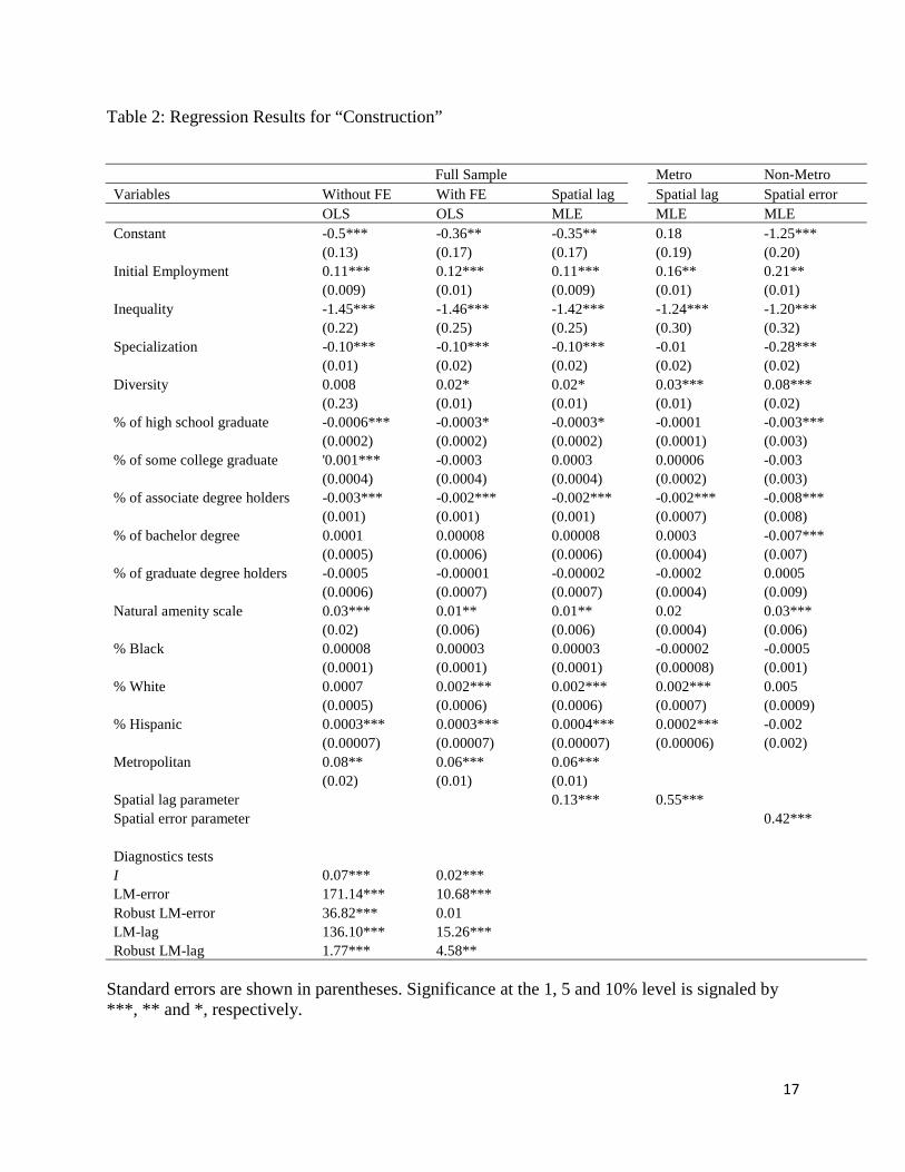
- Construction

Considering the full sample and sub-samples, the correlation between employment growth and

family income inequality appears to be negative and significant. The direction of the association

is consistent across all models and the magnitude of the correlation is slightly higher for models

estimated with the full sample. Urban and rural locations show similar correlation between 2 We only present results of the appropriate spatial process. Using the spatial diagnostic tests from OLS estimation, the appropriate spatial process is determined.

10

employment growth and family income inequality in that industry. The spatial parameters are

significant in all spatial regressions. Table 2 shows results of the estimation.


- Manufacturing

Under the full sample, the correlation between employment growth and family income inequality

is negative and insignificant for both models with and without fixed effects. In both cases, the

spatial diagnostics tests indicate a spatial lag model as the appropriate specification of the

underlying spatial process. The correlation is also negative and insignificant in the spatial lag

model, yet the spatial lag parameter is statistically significant. The urban and rural samples show

opposite association between employment growth and family income inequality, with higher

magnitude for urban sample. The regression results are presented in Table 3.


- Retail Trade

A negative and insignificant correlation is observed between employment growth and inequality

when the model is estimated with full sample. The spatial lag parameter is significant, indicating

a spatial dependence in the employment growth process. In sub-samples, the correlation is

significant for both urban and rural samples, with similar magnitude but opposite direction.

Estimation results are presented in Table 4.


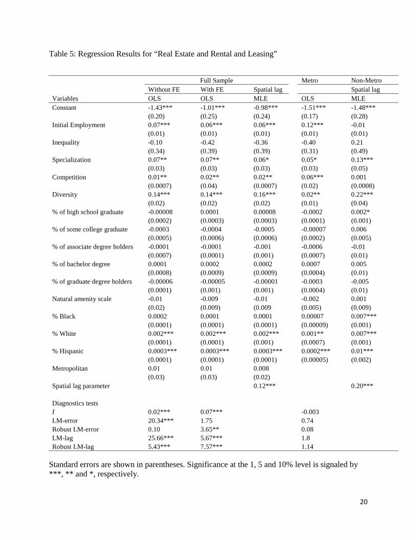
- Real Estate, Rental and Leasing

For all models estimated under full sample and sub-samples, the correlation between

employment growth and family income inequality is insignificant. In both cases, a spatial lag

model was appropriate, and the spatial lag parameters are significant. Table 5 shows the results

of these estimations.


11

- Professional Scientific and Technical Services

Considering the full sample, OLS estimation of the model with/ and without state fixed effects

shows a negative and significant correlation between employment growth and inequality. The

diagnostic statistics for both models strongly support the spatial lag model as the appropriate

spatial process. However, even though the direction of the correlation remains consistent in the

spatial lag model, it is no longer significant. In the sub-sample estimation, both urban and rural

samples show a negative association, but the correlation is only significant for the urban sample.



- Accommodation and Food Services

Using OLS on the full sample, the correlation between employment growth and family income

inequality is only significant when states fixed effects are accounted for. A negative association

is observed. The spatial lag model indicates a negative and significant correlation of similar

magnitude to the model with fixed effects. In sub-samples, the correlation appears to be

insignificant for both urban and rural samples. The spatial parameters are significant across all

spatial models. Table 7 shows the estimation results.


- Educational Services

Considering the full sample, a positive and significant correlation is observed between

employment growth and inequality for the spatial lag model. The spatial lag parameter is also

significant. With regards to sub-samples, the association is only insignificant for urban samples.



12

6. Conclusion

This paper investigates the association between employment growth and family income

inequality for 8 two-digit industries of the NAICS classification. For each of these industries, we

estimated a model where employment growth depends on family income inequality, and a

number of control variables which capture potential agglomeration economies, demographic

composition and natural amenities. These models are estimated using spatial econometrics

techniques. Results indicate that there is no association between employment growth and family

income inequality in the Agriculture, Forestry, Fishing and Hunting sector and the Real Estate,

Rental and Leasing sector. However, family income inequality consistently shows a negative

effect on employment growth in the construction sector. Results are mixed for the following

sectors: Manufacturing; Retail Trade; Professional Scientific and Technical Services;

Accommodation and Food Services; and Educational Services. The results also confirm previous

conclusion of Fallah and Partridge (2007) in which mixed results were obtained when

differentiating between rural and urban regions.

Reference

Aghion, P., Caroli, E. and Garcia-Penalosa, C. (1999). “Inequality and Economic Growth: The

Perspective of the New Growth Theories” Journal of Economic Literature 37:1615–1660

Alesina, A. and Rodrik, D. (1994). “Redistributive Politics and Economics Growth” Quarterly

Journal of Economics 109:465–490.

Arrow, K.J. (1962). “The Economic Implication of Learning by Doing” Review of Economic

Studies 29:155–173.

Bell, L and Freeman, R. (2001). “The Incentive for Working Hard: Explaining Hours Worked

Differences in the US and Germany” Labour Eonomics 2:181–202.

Berg, I (1970). “ The Great Training Robbery” New York: Praeger.

Campano, S. and Salvatore, D. (2006). “Income Distribution” Oxford: Oxford University Press.

Clarke, G.R. (1995). “More Evidence on Income Distribution and Growth” Journal of

Development Economics 47:403–427.

13

Deininger, K. and Squire, L. (1998). “New Ways of Looking at Old Issue: Inequality and

Growth” Journal of Development Economics 57:259–87.

De Dominicis, L., Florax, R.J.G.M. and de Groot, H. (2008). “A Meta-Analysis on the

Relationship between Income Inequality and Economic Growth” The Scottish Journal

of Political Economy 55:654–682.

Ertur, C. and Koch, W. (2007). “Growth, Technological Interdependence and Spatial

Externalities: Theory and Evidence” Journal of Applied Econometrics 22:1033–1062.

Fallah, B. and Partridge, M. (2007). “The Elusive Inequality-Economic Growth Relationship:

are there Differences between Cities and the Countryside?” The Annals of regional

Science 41:375–400.

Forbes, K.J. (2000). “A Reassessment of the Relationship between Inequality and Growth”

American Economic Review 90:869–87.

Glaeser, E. Kallal, H.D. and Scheinkman, A.J. (1992). “Growth in Cities”, Journal of Political

Economy 100: 1126–1152.

Howell, D.R. and Wolff, E.N. (1991). “Trends in the Growth and Distribution of Skills in the

U.S. Workplace, 1960-1985” Industrial and Labor Relations Review 44:487–502.

Jacobs, J. (1969). “The Economy of Cities” Random House, New York, NY.

Kuznets, S. (1955). “Economic Growth and Income Inequality." American Economic Review

45:1–28.

Lazear, E.P. (2000). “Performance Pay and Productivity” American Economic Review 90:1346–

1361.

Li, H. and Zou, H. (1998). “Income Inequality is not Harmful for Growth: Theory and Evidence”

Review of Development Economics 2:318–34.

Mangan, J and Trendle, B. (2002). “The Changing Skills Composition of Employment in

Queensland” Working paper No.6.

Marshal, A. (1890). “Principles of Economics” London: Macmillan.

14

McCann, P. (2001). “Urban and Regional Economics” Oxford University Press.

McGranahan, D. (1999). “Natural Amenities Drive Rural Population Change” Agricultural

Economic Report No. (AER781) 32 pp.

Mirrlees, J.A. (1971). “An Exploration in the Theory of Optimum Income Taxation” Review of

Economic Studies 38:175–208.

Novotny, J. (2007). “On the Measurement of Regional Inequality: Does Spatial Dimension of

Income Inequality matter?” Annals of Regional Science 41:563–580.

Okun, A. (1975). “Equality and Efficiency: The Big Trade-off” Washington D.C. Brookings

Institution.

Panizza, U. (2002) “Income Inequality and Economic Growth: Evidence from American Data”

Journal of Economic Growth 7:25–41.

Parent, O. and Riou, S. (2005). “Bayesian Analysis of Knowledge Spillovers in European

Regions” Journal of Regional Science 45:747–775.

Perotti, R. (1996). “Growth, Income Distribution and Democracy: What Data Say” Journal of

Economic Growth 1:149–1187.

Persson, T. and Tabellini, G. (1994). “Is Inequality Harmful for Growth? American Economic

Review 84:600–621.

Rey, S.J. and Montouri, B.D. (1999). “U.S. Regional Income Convergence: A Spatial Econo-

metric Perspective” Regional Studies 33:143–156.

Rey , S.J. (2001). “Spatial Analysis of Regional Income Inequality” Western Regional Science

Association Meetings. Montery, California. February.

Romer, P. (1986). “Increasing Returns and Long-Run Growth” Journal of Political Economics

94:1002–1026.

Schweitzer, M. (1997). “Workforce Composition and Earning Inequality” Economic review

Q2:13–24.

15

Siebert, H. (1998). “Commentary: Economic Consequences of Income Inequality.” Symposium

of the Federal Reserve Bank of Kansas City on Income Inequality, Issues and Policy

Options 265–281.

16

Table 1: Regression Results for “Agriculture, Forestry, Fishing and Hunting”

Full Sample Metro Non-Metro

Without FE With FE Spatial lag Spatial lag Spatial lag Variables OLS OLS MLE MLE MLE Constant -0.48*** -0.53*** -0.48*** -0.45*** -0.19**

(0.07) (0.08) (0.08) (0.12) (0.10) Initial Employment 0.03*** 0.03*** 0.03*** 0.05*** -0.0008

(0.004) (0.005) (0.005) (0.007) (0.007) Inequality -0.06 -0.07 -0.07 -0.27 0.05

(0.10) (0.10) (0.11) (0.20) (0.12) Specialization 0.0001 -0.001 -0.001 0.0009 0.001

(0.001) (0.001) (0.001) (0.002) (0.001) Competition -0.004*** -0.003*** -0.003*** -0.003 -0.005***

(0.001) (0.001) (0.001) (0.003) (0.001) Diversity -0.005 -0.007 -0.007 -0.01 0.009

(0.006) (0.006) (0.006) (0.008) (0.01) % of high school graduate -0.0003*** -0.0002*** -0.0002*** -0.0003*** 0.0002

(0.00008) (0.0001) (0.00009) (0.0001) (0.0004) % of some college graduate 0.0008*** 0.0004*** 0.0004*** 0.0005*** 0.002**

(0.0002) (0.0002) (0.0001) (0.0002) (0.001) % of associate degree holders -0.001*** -0.0003 -0.0003 -0.001** -0.003*

(0.0004) 0.0004) (0.0004) (0.0005) (0.003) % of bachelor degree -0.0006*** -0.0004* -0.0004* -0.0004** -0.004**

(0.0002) (0.0002) (0.0002) (0.0003) (0.002) % of graduate degree holders 0.0009*** 0.0008 0.0007*** 0.0009*** 0.004

(0.0003) (0.0003) (0.0003) (0.0003) (0.003) Natural amenity scale -0.02 -0.003 -0.003 -0.005** -0.003**

(0.001) (0.003) (0.002) (0.003) (0.002) % Black -0.0001*** -0.00009* -0.00009* -0.00008 -0.001***

(0.00005) (0.00005) (0.00005) (0.00006) (0.0004) % White 0.0001*** 0.001*** 0.001*** 0.0004 0.001***

(0.0002) (0.0003) (0.0003) (0.0005) (0.0003) % Hispanic 0.00001 -0.00001 -0.00005 0.00004 0.001

(0.00003) (0.00003) (0.00003) (0.00004) (0.0007) Metropolitan -0.01* -0.01* -0.01*

(0.008) (0.008) (0.008) Spatial lag parameter 0.15*** 0.34*** 0.32***

Diagnostics tests I 0.05*** 0.01*** LM-error 67.52*** 7.75** Robust LM-error 0.2 0.0017 LM-lag 79.50*** 8.85** Robust LM-lag 12.19*** 1.10

Standard errors are shown in parentheses. Significance at the 1, 5 and 10% level is signaled by ***, ** and *, respectively.

17

Table 2: Regression Results for “Construction”

Full Sample Metro Non-Metro Variables Without FE With FE Spatial lag Spatial lag Spatial error OLS OLS MLE MLE MLE Constant -0.5*** -0.36** -0.35** 0.18 -1.25***

(0.13) (0.17) (0.17) (0.19) (0.20) Initial Employment 0.11*** 0.12*** 0.11*** 0.16** 0.21**

(0.009) (0.01) (0.009) (0.01) (0.01) Inequality -1.45*** -1.46*** -1.42*** -1.24*** -1.20***

(0.22) (0.25) (0.25) (0.30) (0.32) Specialization -0.10*** -0.10*** -0.10*** -0.01 -0.28***

(0.01) (0.02) (0.02) (0.02) (0.02) Diversity 0.008 0.02* 0.02* 0.03*** 0.08***

(0.23) (0.01) (0.01) (0.01) (0.02) % of high school graduate -0.0006*** -0.0003* -0.0003* -0.0001 -0.003***

(0.0002) (0.0002) (0.0002) (0.0001) (0.003) % of some college graduate '0.001*** -0.0003 0.0003 0.00006 -0.003

(0.0004) (0.0004) (0.0004) (0.0002) (0.003) % of associate degree holders -0.003*** -0.002*** -0.002*** -0.002*** -0.008***

(0.001) (0.001) (0.001) (0.0007) (0.008) % of bachelor degree 0.0001 0.00008 0.00008 0.0003 -0.007***

(0.0005) (0.0006) (0.0006) (0.0004) (0.007) % of graduate degree holders -0.0005 -0.00001 -0.00002 -0.0002 0.0005

(0.0006) (0.0007) (0.0007) (0.0004) (0.009) Natural amenity scale 0.03*** 0.01** 0.01** 0.02 0.03***

(0.02) (0.006) (0.006) (0.0004) (0.006) % Black 0.00008 0.00003 0.00003 -0.00002 -0.0005

(0.0001) (0.0001) (0.0001) (0.00008) (0.001) % White 0.0007 0.002*** 0.002*** 0.002*** 0.005

(0.0005) (0.0006) (0.0006) (0.0007) (0.0009) % Hispanic 0.0003*** 0.0003*** 0.0004*** 0.0002*** -0.002

(0.00007) (0.00007) (0.00007) (0.00006) (0.002) Metropolitan 0.08** 0.06*** 0.06***

(0.02) (0.01) (0.01) Spatial lag parameter 0.13*** 0.55*** Spatial error parameter 0.42***

Diagnostics tests I 0.07*** 0.02*** LM-error 171.14*** 10.68*** Robust LM-error 36.82*** 0.01 LM-lag 136.10*** 15.26*** Robust LM-lag 1.77*** 4.58**


18

Table 3: Regression Results for “Manufacturing”


Variables Without FE With FE Spatial lag Spatial lag Spatial lag OLS OLS MLE MLE MLE Constant -0.85*** -0.61** -0.61* 2.59** -1.80***

(0.24) (0.32) (0.31) (0.30) (0.35) Initial Employment 0.07*** 0.05*** 0.04*** -0.16*** 0.10***

(0.01) (0.01) (0.01) (0.02) (0.02) Inequality -0.09 -0.74 -0.70 -2.06** 1.01*

(0.45) (0.50) (0.50) (0.51) (0.62) Specialization -0.28*** -0.27*** -0.26*** -0.17*** -0.27***

(0.03) (0.03) (0.03) (0.03) (0.04) Competition -0.007*** -0.007*** -0.007*** -0.08 -0.004**

(0.001) (0.002) (0.002) (0.01) (0.002) Diversity -0.01 0.007 0.01 0.07*** 0.07

(0.02) (0.02) (0.03) (0.02) (0.06) % of high school graduate -0.0009*** -0.0007* -0.0007* 0.00005 -0.001

(0.0003) (0.0004) (0.0004) (0.0002) (0.002) % of some college graduate 0.002*** 0.0001 0.0001 0.0008 0.008

(0.0007) (0.0008) (0.0008) (0.0004) (0.006) % of associate degree holders -0.002 -0.0001 -0.0009 0.001 -0.01

(0.001) (0.002) (0.002) (0.001) (0.01) % of bachelor degree -0.0008 -0.0008 -0.0006 0.0004 0.005

(0.001) (0.001) (0.001) (0.0007) (0.01) % of graduate degree holders -0.0007 -0.0001 -0.0001 -0.0008 -0.02

(0.001) (0.001) (0.001) 0.0008 (0.01) Natural amenity scale -0.03*** 0.01 0.01 0.002 -0.05***

(0.007) (0.02) (0.01) (0.007) (0.01) % Black -0.0001 -0.00004 -0.00004 -0.0002 -0.0006

(0.0002) (0.0002) (0.0002) (0.0001) (0.002) % White -0.005*** -0.005*** -0.005*** 0.0004*** 0.007

(0.001) (0.001) (0.001) (0.001) (0.001) % Hispanic 0.0003*** 0.0003*** 0.0003*** 0.00005 0.01***

(0.001) (0.0001) (0.0001) (0.0001) (0.003) Metropolitan 0.12*** 0.10*** 0.09***


Diagnostics tests I 0.04*** 0.01*** LM-error 73.90*** 11.56*** Robust LM-error 1.22 0.7 LM-lag 89.74*** 15.10*** Robust LM-lag 17.05*** 4.24***


19

Table 4: Regression Results for “Retail Trade”

Full Sample Metro Non-Metro Variables Without FE With FE Spatial lag Spatial error Spatial lag OLS OLS MLE MLE MLE Constant -1.71** -1.80** 1.70*** -1.27*** -1.77***

(0.12) (0.15) (0.15) (0.24) (0.16) Initial Employment 0.13*** 0.13*** 0.12*** 0.12*** 0.14***

(0.008) (0.008) (0.008) (0.01) (0.01) Inequality 0.49*** 0.64 0.10 -1.11** 1.09***

(0.20) (0.20) (0.20) (0.36) (0.23) Specialization -0.09*** -0.13*** -0.12*** -0.12** -0.21***

(0.003) (0.003) (0.003) (0.05) (0.04) Competition -0.02** -0.02* -0.01* -0.02 -0.01

(0.01) (0.01) (0.01) (0.03) (0.01) Diversity 0.05*** 0.06*** 0.06*** 0.02* 0.14***

(0.01) (0.01) (0.01) (0.01) (0.02) % of high school graduate -0.0004*** -0.0003** -0.0003** -0.0003** -0.0008

(0.0001) (0.0001) (0.0001) (0.0001) (0.0008) % of some college graduate 0.0003 0.0004 0.0002 0.0003** 0.0003

(0.0003) (0.0003) (0.0003) (0.0003) (0.0002) % of associate degree holders -0.002*** -0.002*** -0.002*** -0.002** -0.01**

(0.0008) (0.0009) (0.0008) (0.0009) (0.005) % of bachelor degree '0.0002 '0.00001 '0.00003 0.00001 0.0004


(0.0005) (0.0005) (0.0005) (0.0005) (0.006) Natural amenity scale 0.02*** 0.03*** 0.03*** 0.02*** 0.02***

(0.003) (0.005) (0.005) (0.007) (0.004) % Black -0.00007 -0.0001 -0.0001 0.00003 0.002***

(0.0001) (0.0001) (0.0001) (0.0001) (0.004) % White 0.0009** 0.001*** 0.001*** 0.005*** -0.001**

(0.0004) (0.0005) (0.0005) (0.0009) (0.0006) % Hispanic 0.0004*** 0.0004*** 0.0004*** 0.0003*** -0.002

(0.00006) (0.00006) (0.00006) (0.00007) (0.001) Metropolitan 0.03** 0.008** 0.004**


Diagnostics tests I 0.08*** 0.01*** LM-error 223.87*** 6.83*** Robust LM-error 35.84*** 13.48*** LM-lag 227.56*** 39.61*** Robust LM-lag 39.52** 46.26***


20

Table 5: Regression Results for “Real Estate and Rental and Leasing”


Without FE With FE Spatial lag Spatial lag Variables OLS OLS MLE OLS MLE Constant -1.43*** -1.01*** -0.98*** -1.51*** -1.48***

(0.20) (0.25) (0.24) (0.17) (0.28) Initial Employment 0.07*** 0.06*** 0.06*** 0.12*** -0.01

(0.01) (0.01) (0.01) (0.01) (0.01) Inequality -0.10 -0.42 -0.36 -0.40 0.21

(0.34) (0.39) (0.39) (0.31) (0.49) Specialization 0.07** 0.07** 0.06* 0.05* 0.13***

(0.03) (0.03) (0.03) (0.03) (0.05) Competition 0.01** 0.02** 0.02** 0.06*** 0.001

(0.0007) (0.04) (0.0007) (0.02) (0.0008) Diversity 0.14*** 0.14*** 0.16*** 0.02** 0.22***

(0.02) (0.02) (0.02) (0.01) (0.04) % of high school graduate -0.00008 0.0001 0.00008 -0.0002 0.002*

(0.0002) (0.0003) (0.0003) (0.0001) (0.001) % of some college graduate -0.0003 -0.0004 -0.0005 -0.00007 0.006

(0.0005) (0.0006) (0.0006) (0.0002) (0.005) % of associate degree holders -0.0001 -0.0001 -0.001 -0.0006 -0.01

(0.0007) (0.0001) (0.001) (0.0007) (0.01) % of bachelor degree 0.0001 0.0002 0.0002 0.0007 0.005


(0.0001) (0.001) (0.001) (0.0004) (0.01) Natural amenity scale -0.01 -0.009 -0.01 -0.002 0.001

(0.02) (0.009) (0.009 (0.005) (0.009) % Black 0.0002 0.0001 0.0001 0.00007 0.007***

(0.0001) (0.0001) (0.0001) (0.00009) (0.001) % White 0.002*** 0.002*** 0.002*** 0.001** 0.007***

(0.0001) (0.0001) (0.001) (0.0007) (0.001) % Hispanic 0.0003*** 0.0003*** 0.0003*** 0.0002*** 0.01***

(0.0001) (0.0001) (0.0001) (0.00005) (0.002) Metropolitan 0.01 0.01 0.008

(0.03) (0.03) (0.02) Spatial lag parameter 0.12*** 0.20***

Diagnostics tests I 0.02*** 0.07*** -0.003 LM-error 20.34*** 1.75 0.74 Robust LM-error 0.10 3.65** 0.08 LM-lag 25.66*** 5.67*** 1.8 Robust LM-lag 5.43*** 7.57*** 1.14


21

Table 6: Regression Results for “Professional Scientific and Technical Services”

Full Sample Metro Non-Metro Variables Without FE With FE Spatial lag Spatial error Spatial lag OLS OLS MLE MLE MLE Constant -2.97*** -2.49*** -2.71*** -2.16*** -2.95***

(0.22) (0.30) (0.22) (0.30) (0.31) Initial Employment 0.28*** 0.26*** 0.25*** 0.23*** 0.23***

(0.01) (0.01) (0.15) (0.01) (0.02) Inequality -0.74** -1.20*** -0.52 -1.17*** -0.40

(0.37) (0.42) (0.37) (0.50) (0.50) Specialization -0.12*** -0.12*** -0.10*** -0.16*** -0.05

(0.04) (0.04) (0.43) (0.06) (0.06) Competition 0.16*** 0.16*** 0.17*** 0.09** '0.18***

(0.01) (0.01) (0.01) (0.03) (0.02) Diversity 0.06*** 0.08*** 0.06*** -0.007 0.21***

(0.02) (0.02) (0.02) (0.03) (0.04) % of high school graduate -0.0008*** -0.0005*** -0.0009*** -0.006*** -0.0002

(0.0003) (0.0003) (0.0003) (0.0002) (0.001) % of some college graduate -0.000009 -0.0004 -0.0001 0.0002 0.007

(0.0006) (0.0007) (0.0006) (0.0004) (0.005) % of associate degree holders -0.001 -0.001 -0.001 -0.001 -0.02

(0.001) (0.001) (0.001) (0.001) (0.01) % of bachelor degree -0.0001 -0.0005 -0.0004 -0.0001 -0.01

(0.0009) (0.001) (0.0009) (0.0006) (0.01) % of graduate degree holders -0.0005 -0.00007 -0.0006 0.0002 0.01

(0.001) (0.001) (0.001) (0.0007) (0.01) Natural amenity scale 0.02*** 0.01 0.02 0.01*** 0.02***

(0.006) (0.009) (0.006) (0.008) (0.008) % Black 0.0004** 0.0002 0.0003** 0.0002 0.004***

(0.0001) (0.0002) (0.0001) (0.0001) (0.001) % White 0.001* 0.003*** 0.001*** 0.0003*** 0.002*

(0.0008) (0.001) (0.0008) (0.0001) (0.001) % Hispanic 0.0005*** 0.0005*** 0.0005*** 0.0002*** 0.005

(0.0001) (0.0001) (0.0001) (0.0001) (0.003) Metropolitan 0.05* 0.02 0.04


Diagnostics tests I 0.04*** 1.23*** LM-error 65.32*** 4.96** Robust LM-error 4.14** 4.71** LM-lag 82.66*** 19.03*** Robust LM-lag 21.48*** 18.78***


22

Table 7: Regression results for “Accommodation and Food Services”


Without FE With FE Spatial lag Spatial lag Spatial lag Variables OLS OLS MLE MLE MLE Constant -0.26* -0.1958 -0.22 0.71*** -0.44***

(0.15) (0.18) (0.17) (0.25) (0.18) Initial Employment 0.05*** 0.045*** 0.04*** -0.01* 0.04***

(0.01) (0.01) (0.009) (0.01) (0.01) Inequality 0.35 -0.53* -0.52** -0.45 0.05

(0.25) (0.28) (0.27) (0.42) (0.30) Specialization -0.21*** -0.16*** -0.15*** -0.30*** -0.15***

(0.02) (0.02) (0.02) (0.03) (0.02) Competition 0.001 0.001 0.001 -0.10*** 0.002***

(0.02) (0.001) (0.001) (0.01) (0.001) Diversity 0.05*** 0.06*** 0.06*** 0.04** 0.11**

(0.02) (0.016) (0.02) (0.01) (0.02) % of high school graduate -0.0002 -0.00004 -0.00002 -0.0001 0.00008

(0.0002) (0.0002) (0.0002) (0.0002) (0.001) % of some college graduate 0.0003 0.0002 0.0001 0.0003 -0.001

(0.0004) (0.0005) (0.0004) (0.0004) (0.003) % of associate degree holders -0.004*** -0.003* -0.003*** -0.002*** -0.01**

(0.001) (0.001) (0.001) (0.001) (0.007) % of bachelor degree 0.0008 0.0001 0.0001 0.0003 0.001

(0.0006) (0.0007) (0.0006) (0.0005) (0.0006) % of graduate degree holders -0.001 -0.0001 -0.0001 -0.0004*** 0.0004

(0.0007) (0.0008) (0.0007) (0.0006) (0.0008) Natural amenity scale 0.038*** 0.032*** 0.03*** 0.02*** 0.03***

(0.022) (0.007) (0.006) (0.006) (0.005) % Black 0.0001 -0.00002 -0.00001 0.00003 0.001***

(0.0001) (0.0001) (0.0001) (0.0001) (0.001) % White 0.00001 0.003*** 0.002*** 0.002* 0.001***

(0.0006) 0.001 (0.0007) (0.001) (0.001) % Hispanic 0.0003*** 0.0003*** 0.0002*** 0.0002*** 0.002

(0.0001) (0.0001) (0.00009) (0.00009) (0.001) Metropolitan 0.1425*** 0.097*** 0.09***


Diagnostics tests I 0.1*** 0.18*** LM-error 329.80*** 10.74*** Robust LM-error 2.71*** 3.38* LM-lag 373.07*** 20.28*** Robust LM-lag 45.98*** 12.92***


23

Table 8: Regression Results for “Educational Services”

Full Sample Metro Non-Metro Variables Without FE With FE Spatial lag Spatial error Spatial lag OLS OLS MLE MLE MLE Constant 0.001 -0.20 -0.06 0.49** -1.14

(0.02) (0.23) (0.18) (0.28) (0.24) Initial Employment -0.003 0.01** -0.005 -0.01 -0.01***

(0.004) (0.004) (0.004) (0.008) (0.005) Inequality 0.10 0.67* 0.19*** -0.37** 0.28

(0.3) (0.4) (0.34) (0.54) (0.44) Specialization -0.04*** -0.03*** -0.03*** -0.01*** -0.04***

(0.01) (0.01) (0.01) (0.02) (0.01) Competition 0.000007 0.00000004 0.00001 0.008 -0.00004

(0.0002) (0.0002) (0.0001) (0.01) (0.0002) Diversity 0.1*** 0.08*** 0.09*** 0.08*** 0.001

(0.02) (0.02) (0.02) (0.01) (0.03) % of high school graduate 0.00005 0.0002 0.0001 0.0001 0.0001

(0.0003) (0.0003) (0.0002) (0.0002) (0.0001) % of some college graduate -0.0004 -0.0002 -0.0002 0.0003 -0.001

(0.0005) (0.0006) (0.0005) (0.0005) (0.004) % of associate degree holders 0.001 -0.0004 0.0003 0.0004 -0.01

(0.001) (0.003) (0.001) (0.001) (0.01) % of bachelor degree 0.0005 0.001 0.0005 0.0005 0.02**


(0.001) (0.001) (0.0009) 0.0008 (0.01) Natural amenity scale 0.01** 0.0008 0.007 0.009 0.007

(0.005) (0.009) (0.005) (0.008) (0.007) % Black -0.00002 -0.0002 -0.0004 -0.0001 0.001

(0.0002) (0.0002) (0.0001) (0.0001) (0.002) % White -0.002*** -0.002* -0.001*** -0.006*** -0.001

(0.0008) (0.001) (0.0001) (0.001) (0.002) % Hispanic -0.0001 -0.00002 -0.0001 0.0001 -0.005***

(0.0001) (0.0001) (0.0001) (0.0001) (0.002) Metropolitan 0.09*** 0.09*** 0.09***


Diagnostics tests I 0.02*** 0.002*** LM-error 17.27*** 0.11 Robust LM-error 2.70* 0.13 LM-lag 23.78*** 0.07 Robust LM-lag 9.21*** 0.08


Date post:	29-Apr-2018
Category:	Documents
Upload:	trinhkiet
View:	215 times
Download:	1 times

Employment Growth and Income Inequality: Accounting...

Documents