WP/15/28

Employment Impacts of Upstream Oil and Gas Investment in the United States

Prepared by Mark Agerton, Peter Hartley, Kenneth Medlock III and Ted Temzelides

© 2015 International Monetary Fund WP/15/28

IMF Working Paper

Research Department

Employment Impacts of Upstream Oil and Gas Investment in the United States

Prepared by Mark Agerton, Peter Hartley, Kenneth B. Medlock III and Ted Temzelides1

Authorized for distribution by Prakash Loungani

February 2015

Abstract

Technological progress in the exploration and production of oil and gas during the 2000s has led to a boom in upstream investment and has increased the domestic supply of fossil fuels. It is unknown, however, how many jobs this boom has created. We use time-series methods at the national level and dynamic panel methods at the state-level to understand how the increasein exploration and production activity has impacted employment. We find robust statistical support for the hypothesis that changes in drilling for oil and gas as captured by rig-counts doin fact, have an economically meaningful and positive impact on employment. The strongest impact is contemporaneous, though months later in the year also experience statistically and economically meaningful growth. Once dynamic effects are accounted for, we estimate that an additional rig-count results in the creation of 37 jobs immediately and 224 jobs in the long run, though our robustness checks suggest that these multipliers could be bigger.

JEL Classification Numbers: J-21

Keywords: Employment

Authors E-Mail Addressess: magerton@rice.edu; hartley@rice.edu; medlock@rice.edu; tedt@rice.edu

1 Center for Energy Studies, James A. Baker III Institute for Public Policy, Rice University

This Working Paper should not be reported as representing the views of the IMF. The views expressed in this Working Paper are those of the author(s) and do not necessarily represent those of the IMF or IMF policy. Working Papers describe research in progress by the author(s) and are published to elicit comments and to further debate.

2

Contents Page

I. Introduction ............................................................................................................................4 

II. Literature Review ..................................................................................................................6 

III. Rig-counts ............................................................................................................................8 

IV. Vector Autoregression Model ..............................................................................................9 A. Data and Identification ............................................................................................10 B. Estimation and Results ............................................................................................11 

V. State Dynamic Panel Model ................................................................................................14 

VI. State Panel Results .............................................................................................................16 

VII. Four Robustness Checks ..................................................................................................18 A. Lag Lengths .............................................................................................................18 B. Outliers ....................................................................................................................19 C. Structural Breaks .....................................................................................................19 D. Population Scaling ..................................................................................................21 

VIII. Conclusion ......................................................................................................................22 

References ................................................................................................................................23 Figures 1. Cumulative Employment Growth (Percent) Relative to National .......................................5 2. Labor, Capital and Prices in Oil & Gas (Standardized Variables) .....................................9 3. COIRFs for One-Standard Deviation Rig-Count Shocks and Employment Responses in SVARs (95% CI) ........................................................................................12 4. FEVD for Rig-count Shock and Employment Response (95% CI) ..................................12 5. COIRFs for One-standard Deviation Shocks in Oil and Gas SVAR (95% CI) ................13 6. FEVD for Oil and Gas SVAR ............................................................................................14 7. IRF and CIRF for Panel Model ..........................................................................................18 8. IRF and CIRF for Different Lag-lengths ...........................................................................19 9. IRF and CIRF for Rig-Counts Pre and Post 2008..............................................................20

Appendix ..................................................................................................................................25 A. National Data ..........................................................................................................25 B. State Data ................................................................................................................25

Appendix Tables 1. Base Model with Different Standard Errors ......................................................................27 2. Estimated Employment Impact due to Rig-count Changes ...............................................28 3. Different Lag Lengths ........................................................................................................29

3

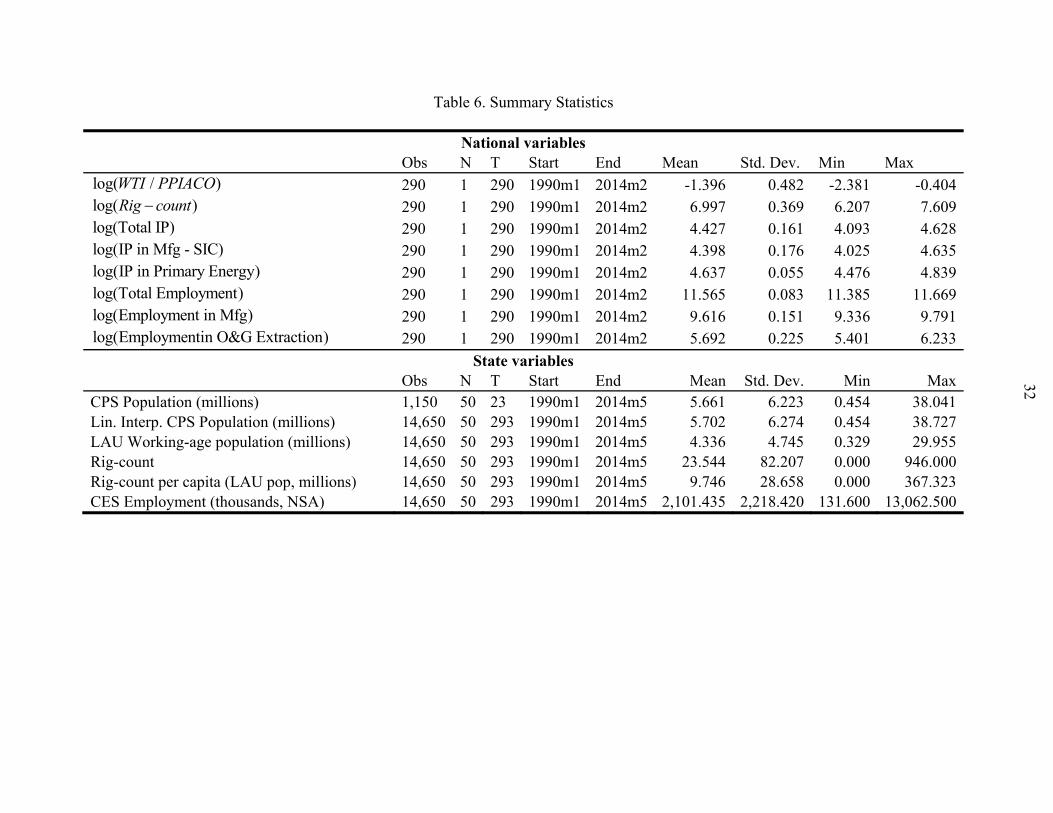
4. Multipliers for Model (1) When Each State is Omitted .....................................................30 5. Per-capita and Log Models with Different Population Scaling .........................................31 6. Summary Statistics .............................................................................................................32 Appendix Figures 10. Map of US Shale Gas and Tight Oil Plays ........................................................................33 11. Rig-counts Per Million Working-age People .....................................................................34 12. Rig-counts (levels) ............................................................................................................35

4

I. INTRODUCTION

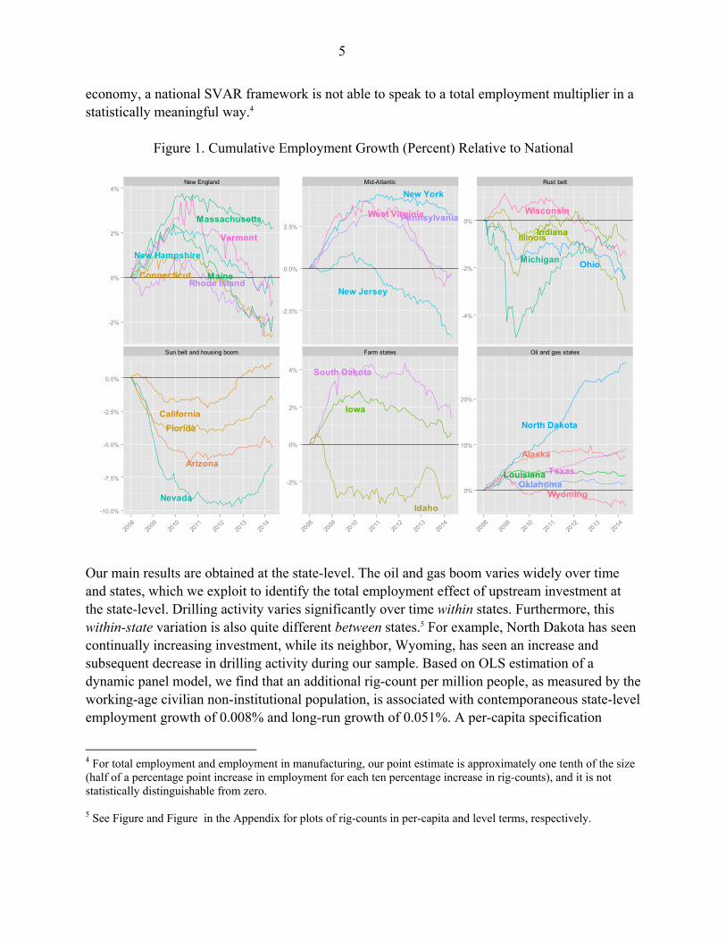
The development of shale has created a new boom in the oil and gas industry.2 There are also indications that it has led to economic revitalization in places like North Dakota, Texas, Alberta, West Pennsylvania, and Louisiana. This revolutionary increase in the production of oil and natural gas has led to a discussion about its potential effects on employment. Anecdotal evidence about the employment experience of different states over the last recession suggests that such effects may indeed be present. Figure 1 shows cumulative employment growth of various states (in approximate percentage terms) since January 2008 versus the national average.3 The base year roughly coincides with both a severe drop in employment due to recession and the beginning of the boom in shale gas and tight oil production. The dominant feature of the plot showing oil and gas states is North Dakota, which has seen blistering employment growth (note the scale). In fact, North Dakota, Texas, Alaska and Louisiana had the highest cumulative employment growth from 2008 through 2013 out of all states—27.4, 7.86, 5.80 and 3.68 percent, respectively. In 2013, all were top producers of oil and gas. While the aggregate effect on employment from developing different energy sources is an important question, it cannot be readily answered in the context of traditional dynamic general equilibrium macroeconomic models. As these models assume market clearing, they cannot account for variations in unemployment rates and, thus, are not well suited to study the employment consequences of alternative government policies or other shocks. Input-Output (I/O) analysis, which is commonly used in economic impact studies, is also poorly suited to answer our research question. It cannot incorporate induced price changes or substitution between inputs in production, which means that multipliers are usually overstated. Furthermore, as Kinnaman (2011) points out, because these studies are calibrated with data on a region’s existing industries, predicting the impact of a totally new industry in the region—for example, shale gas in Pennsylvania—is problematic. Our approach is an empirical one. We first consider the interrelationships between real oil prices, national rig-counts, the production of primary energy and employment in the oil and gas extraction industry in a Structural Vector Autoregression (SVAR) at the national level. After 24 months, we estimate that a ten percent increase in rig-counts results in an approximately five percent increase in industry employment. Total changes in employment will depend on the extent to which job gains in oil and gas extraction (and related sectors) are offset by job losses in others as workers change industries. Because energy production is a relatively small portion of the

2 See Figure in the Appendix for an Energy Information Agency (EIA) map of where unconventional oil and gas is located in the continental United States.

3 Following Blanchard and Katz (1992), cumulative employment growth relative to national is calculated as

, 2008 2008log( / ) log( / )it I Jan tEmp Emp NatlEmp NatlEmp .

5

economy, a national SVAR framework is not able to speak to a total employment multiplier in a statistically meaningful way.4

Figure 1. Cumulative Employment Growth (Percent) Relative to National

Our main results are obtained at the state-level. The oil and gas boom varies widely over time and states, which we exploit to identify the total employment effect of upstream investment at the state-level. Drilling activity varies significantly over time within states. Furthermore, this within-state variation is also quite different between states.5 For example, North Dakota has seen continually increasing investment, while its neighbor, Wyoming, has seen an increase and subsequent decrease in drilling activity during our sample. Based on OLS estimation of a dynamic panel model, we find that an additional rig-count per million people, as measured by the working-age civilian non-institutional population, is associated with contemporaneous state-level employment growth of 0.008% and long-run growth of 0.051%. A per-capita specification

4 For total employment and employment in manufacturing, our point estimate is approximately one tenth of the size (half of a percentage point increase in employment for each ten percentage increase in rig-counts), and it is not statistically distinguishable from zero. 5 See Figure and Figure in the Appendix for plots of rig-counts in per-capita and level terms, respectively.

Connecticut Maine

Massachusetts

New Hampshire

Rhode Island

Vermont

New Jersey

New York

PennsylvaniaWest Virginia

IllinoisIndiana

MichiganOhio

Wisconsin

Arizona

California

Florida

NevadaIdaho

Iowa

South Dakota

Alaska

Louisiana

North Dakota

Oklahoma

Texas

Wyoming

New England Mid-Atlantic Rust belt

Sun belt and housing boom Farm states Oil and gas states

-2%

0%

2%

4%

-2.5%

0.0%

2.5%

-4%

-2%

0%

-10.0%

-7.5%

-5.0%

-2.5%

0.0%

-2%

0%

2%

4%

0%

10%

20%

2008

2009

2010

2011

2012

2013

2014

2008

2009

2010

2011

2012

2013

2014

2008

2009

2010

2011

2012

2013

2014

6

suggests that a single rig-count is associated with 37 new jobs in the same month and 224 jobs in the long run. Finally, we also carry out a range of sensitivity analyses that suggest our results are relatively robust to non-spherical errors, different lag-lengths and measures of population. Furthermore, they are neither driven by one state in particular nor are they driven by the pre or post-2008 period only.

II. LITERATURE REVIEW

There are several industry related studies of the employment effects of upstream oil and gas development (T. Considine et al. 2009; T. J. Considine, Watson, and Blumsack 2010; Higginbotham et al. 2010; IHS Global Insight 2011; Murray and Ooms 2008; Scott 2009; Swift, Moore, and Sanchez 2011). Most of them use the Input-Output (I/O) methodology and predict large increases, not only in employment but also in tax revenues and production. Kinnaman (2011) provides a peer-reviewed survey and stinging critique of a number of these. He points out that several assume, perhaps counter-factually, that nearly all windfall gains by households are spent locally and immediately, that most inputs are locally produced and that royalties are accrued locally. By taking an empirical approach, we can infer employment multipliers while remaining agnostic about the parameters underlying consumer and firm behavior. It is important to note that since we examine total employment, our analysis allows for effects of oil and gas development on other industries. Our analysis gives rise to lower multipliers than these I/O studies. For example, Considine et al. (2009) estimate that upstream investment in the Marcellus shale created 29,284 jobs in Pennsylvania in 2008, and their follow-up study estimates that 44,098 jobs were created in 2009 (T. J. Considine, Watson, and Blumsack 2010). We assert that the increase in Pennsylvania rig-counts in 2008 and 2009 immediately created 213 and 1,404 jobs, respectively, and after accounting for dynamic multiplier effects, an ultimate increase of 1,288 and 8,475 jobs (see Table2). The IHS (2011) study finds that the shale gas industry “supported over 600,000 jobs” in 2010 once direct, indirect and induced jobs were summed. Using our multipliers, we find that national changes in rig-counts were associated with a contemporaneous increase of 19,960 jobs, rising to 120,514 jobs when dynamic effects are taken into account.6 Note that 2010 happens to be the largest January to January increase in rig-counts, so the estimates of job growth for 2009 were negative and had larger magnitudes, and those in 2011 were positive but had half of the magnitude. One empirical approach, which we elect not to take, is the treatment-effect design, which is common in labor economics. The first paper to use this design in relation to the employment

6 Applying our state-level multipliers to the national level is problematic since job gains in oil and gas producing states may be offset by losses in other non-producing states, but the calculation is illustrative of the different magnitudes obtained in I/O studies versus our empirical model.

7

impacts of a North American resource boom was Black et al. (2005), which examined the effect of coal booms and busts on county employment in Appalachia. The authors use the presence of large coal reserves as their treatment indicator variable and find modest multiplier effects: for every ten jobs created in the mining sector, 1.74 jobs in the local-goods sector are created, and for a bust, 3.5 local jobs are lost for each ten mining jobs. Weber (2012) uses a similar study design and estimates a triple-difference specification where the treatment is the value of gas production and the instrument used is the percentage of a county covered by shale deposits. He finds that an additional million dollars of natural gas production (resulting from increased price or production) leads to 2.35 additional jobs in the county. In a follow-up study, Weber (Forthcoming) examines the possibility that the unconventional gas boom might lead to a resource curse in rural counties. He finds that an additional 22 billion cubic feet (bcf) of gas production creates 18.5 jobs in each county (7.5 mining jobs and 11.5 non-mining jobs—a multiplier of 1.4 non-mining jobs per mining job), but increased gas production does not lead to crowding out in manufacturing or lower educational levels. Other studies which follow a similar design include a manuscript by Fetzer (2014), who concludes that the natural gas boom does not lead to Dutch Disease and crowding-out of traded goods, possibly due to lower energy prices, and Marchand (2012), who examines the effect of energy booms on Canadian labor market outcomes and also finds modest multiplier effects in the non-trade sector and no crowding out of manufacturing. Our study is different because we use higher-frequency data and exploit the time-series dimension. This allows us to understand the dynamics of job creation, though the use of higher-frequency data may limit our ability to account for lower-frequency, structural shifts in the economy. A recent Baker Institute study (Hartley et al. 2013) considered a similar question to ours using county-level data from Texas. Before the authors allow for cross-county spillovers, they find that each well-count results in 77 short-term jobs, with within-county employment impacts occurring primarily in months zero, one, five and six. They find some evidence that by allowing for county spillovers using a spatial auto-regressive model, the long-run employment effects are almost three times as large. Our research design is a similar, dynamic panel model, and we use a longer dataset (1990 to 2014) for the entire nation. Additionally, where they focus on unconventional oil and gas production, we focus on all oil and gas activity. We find a long-run multiplier that is approximately twice as big as in the basic specification considered by Hartley et al. (2013), but still below the effects the authors estimate after allowing for cross-county spillovers. A 1997 paper by Hooker and Knetter (1997) investigates the employment impact of changes in military spending using a panel of state-level data from 1936—1994. The authors find that exogenous spending shocks (government procurement spending per capita) do lead to changes in employment growth, but the effects of shocks are nonlinear: large, adverse shocks lower employment growth more than smaller ones, while positive shocks also are less effective at increasing employment growth than negative ones at decreasing it. While we use higher-frequency data, we adopt their general model specification, including a set of state-specific intercept terms and time fixed effects as Hooker and Knetter do.

8

Blanchard and Katz (1992) examine the dynamics of regional labor markets using a vector autoregression (VAR) approach with annual state labor-market data. They argue that labor-demand shocks are the primary drivers of changes in employment, unemployment and participation. Furthermore, they provide evidence that migration of workers—not firms—in response to low unemployment rates—not high wages—is the primary mechanism that returns markets to their long-run equilibria. This may mean population (which we use to scale our rig-count variable) is endogenous to upstream investment. To address this, we use a variety of population measures in our robustness checks, including the population in 1990, which is the first year of our dataset and is pre-determined in relation to the shale boom. Finally, Arora and Lieskovsky (2014) examine national economic impacts of the natural gas boom using a Structural Vector Autoregression (SVAR) framework. They find evidence that lower real natural gas prices due to increased supply positively impact industrial production. Furthermore, they find that this effect is greater post-2008 and conclude that the shale gas revolution has altered the relationship of natural gas to the macroeconomy. We estimate a SVAR as well. However, while Arora and Lieskovsky look at the supply side of the economy, we focus on job creation and do not distinguish between the positive supply-side effects of lower energy prices and positive demand-side effects of additional upstream investment.

III. RIG-COUNTS

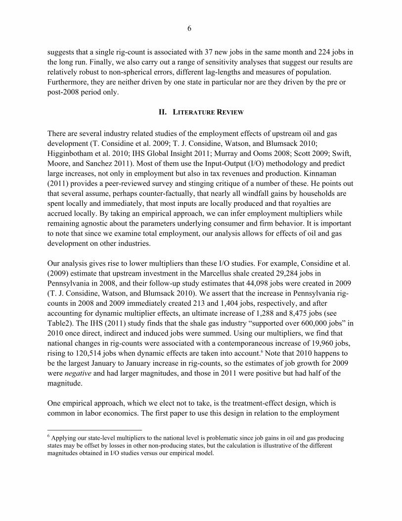
To capture upstream oil and gas investment we use the Baker Hughes rig-counts, which are publicly available on the firm’s website.7 Baker Hughes is a major supplier of oil-field services, and has been publishing reports on the industry since 1944. Each week, the firm surveys rotary rig operators in North America and publishes a count of the number of rigs that are “actively exploring for or developing oil or natural gas” in each state. Many firms and industry analysts use the reports to gauge investment activity in the sector. Weekly state-level data from Baker Hughes begin in 1990, and we average these figures to a monthly frequency. Unfortunately, the weekly (and monthly) data do not provide detail on whether rigs are engaged in unconventional activity or not, so we must use the total number of rigs in each state. Using a similar logic, we choose to include offshore rigs in the total, even though the investment required for offshore wells is very different than onshore wells. Figure2 plots seasonally adjusted national employment in oil and gas extraction plus support activities along with the national average monthly rig-count and the West Texas Intermediate crude benchmark. The three are clearly linked. Plots of the rig-count data in per-capita and level terms are displayed in the Appendix (Figure 11 and Figure 12, respectively).

7 Baker Hughes publishes rig-counts at http://phx.corporate-ir.net/phoenix.zhtml?c=79687&p=irol-reportsother

9

Figure 2. Labor, Capital and Prices in Oil & Gas (Standardized Variables)

Three points are worth making. First, in states with significant exploration and production, there is substantial within-state time series variation in rig-counts which can provide identification of employment impacts. Second, the magnitudes and pattern of variation are different between states. For example, the maximum number of rigs-per month in Texas is 946, while many states have no drilling activity (Connecticut, for example). Third, the states with the highest mean rig-count levels (Texas at 488 and Louisiana at 156) are not those with the highest per-capita count (Wyoming and North Dakota, with are the two highest with 105 and 68 rig-counts per million people respectively). Thus, estimates will be sensitive to whether rig-counts are in level or per-capita terms, and they may be overly-influenced by outliers like Texas and Wyoming. We address the issue of outliers in our robustness checks.

IV. VECTOR AUTOREGRESSION MODEL

While state-level variation in rig-counts and employment may provide more precision in estimating the employment impacts of upstream activity, these estimates cannot account for inter-state effects. On one hand, an energy-boom in one state may induce higher labor-demand and job-creation in another as the boom-state’s income rises. On the other, the boom state may pull workers from nearby states, reducing net job creation at the national level. To address this ambiguity, we model the interaction between real oil price shocks, upstream investment, industrial production and employment. Specifically, we examine three Structural Vector Autoregression (SVAR) models similar to those estimated by Arora and Lieskovsky (2014). Our three models focus on (1) total IP and employment, (2) IP and employment in manufacturing and (3) IP in Primary Energy and employment in oil and gas extraction.

Rig-countsO&G Emp

WTI

-1

0

1

2

3

1990 1995 2000 2005 2010 2015

10

A vector autoregression (VAR) captures the interrelationships between variables that are jointly determined. Unfortunately, shocks to each variable may be correlated, so causation is unidentified without more structure. By imposing restrictions on the shocks, one can identify causal effects of shocks and their relative importance to the system. We follow notation from Lutkehpohl (2005) and define our vector of variables as

log(Real WTI ) log( ) log(IP ) log(Employment )T

t t t t ty Rigs

Since production and employment can both be highly seasonal, and since this seasonality can be deterministic and stochastic in nature, we include monthly dummy variables and specify our VAR in first differences as ( ) ( )t tA L y t u

where 11( ) p

pA L I AL A L is a polynomial in the lag operator, ( )t corresponds to a

month-specific intercept that captures any deterministic seasonality, and is the first-difference operator needed to make the variables stationary. The covariance of the error term [ ]t tE u u may

not be diagonal, so we cannot make causal inference about which shocks drive the system without further restrictions on the model. We choose to use the standard Cholesky decomposition of '[ ]u t tE u u to do this. This corresponds to the following restriction

t tu P

where P is a lower-triangular matrix such that Tu PP and implies a recursive system. We are

primarily interested in the cumulative orthogonalized impulse responses (COIRF), which show the cumulative impact of a one-standard deviation structural shock over time. We calculate the COIRF in period h as

0

ˆh

Tj

j

P

where 1ˆˆ ( ) ( )L I A L

is the VMA representation of the system and ˆj is the coefficient

j -th of the j -th order lag polynomial.

A. Data and Identification

The real domestic price of oil is calculated as the West Texas Intermediate (WTI) spot price scaled by the Producer Price Index (PPI) for all commodities. Oil is globally traded, and its price is set in liquid, international markets. Thus, oil price shocks in time t should be exogenous to the other variables in the model. Rig-counts capture upstream investment activity. Exploration and production firms make decisions based on the expected future profitability of a well, which is

11

determined by drilling costs and expected future oil prices. Drilling changes in time t should respond to oil prices insomuch as they are an indicator of future oil prices; however, since oil and gas production lags drilling activity, drilling changes in t should not drive oil prices in t . By the same token, drilling decisions at time t should not be affected by other contemporaneous economic shocks to industrial production or employment. Three different measures of Industrial Production (not seasonally adjusted) are taken from the Federal Reserve: Total IP, Manufacturing IP (as defined by SIC codes) and IP in Primary Energy. It is generally accepted that employment is a lagging macroeconomic indicator; thus, we order IP before employment. Employment is taken from the BLS Current Establishment Survey and is not seasonally adjusted. Specifically, we use Total Private Non-farm employment, total employment in manufacturing, and the sum of employment in oil and gas extraction plus oil and gas support activities. For more details on data, see the Appendix.

B. Estimation and Results

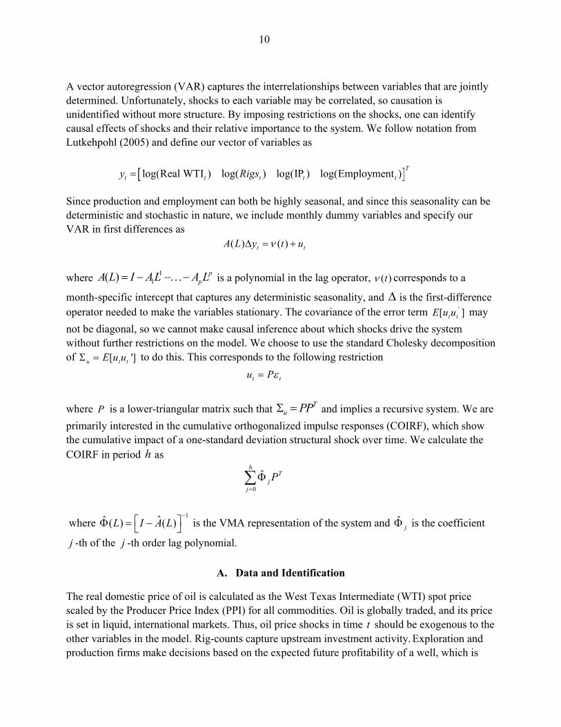
We estimate the three versions of the above model. Lag selection was done using the minimum of the AIC and checking ACFs of residuals to confirm that they are white noise. The three models have twelve, twelve and three lags, respectively. Since both IP and employment are very seasonal, it makes intuitive sense that 12 lags would be required. Fossil-fuel production, however, is generally not seasonal (though its consumption is), so the fact that only three lags are required is not surprising. Figure 3 displays COIRFs from rig-counts to employment for the three models. Since all variables are in logs, the vertical axis represents the approximate percentage change in the response variable with respect to a one standard-deviation shock in the impulse variable. COIRFs from the Total and Manufacturing models do not appear to be statistically significant at almost any lag. Given that these two models leave the majority of the economy unmodeled (in our sample, employment in oil and gas extraction is, on average, just 0.28% of total employment), this finding is not surprising. Our Oil and Gas model, on the other hand shows very positive and significant cumulative employment impacts of additional rig-counts. After re-scaling the COIRF(24) by standard deviation of ,Rigs tu (which is the square-root of the second element of the

diagonal of ˆu and represents the magnitude of a one-standard deviation rig-count shock), we

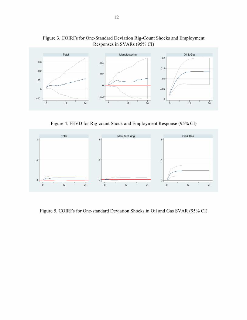
calculate that the a 1.0% increase in rig-counts leads to approximately 0.5% increase in employment in oil and gas extraction.8 , which displays the Forecast Error Variance Decompositions for the impulse-response of rig-counts on employment, shows that rig-count changes do not lead to major changes in employment at the aggregate but do have significant impacts on employment in the oil and gas sector.

8 A similar calculation for the total and manufacturing employment models suggests elasticities that are about 1/10th the size. This could represent a substantial number of jobs, but the estimates are not at all statistically meaningful.

12

Figure 3. COIRFs for One-Standard Deviation Rig-Count Shocks and Employment

Responses in SVARs (95% CI)

Figure 4. FEVD for Rig-count Shock and Employment Response (95% CI)

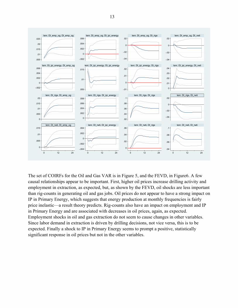
Figure 5. COIRFs for One-standard Deviation Shocks in Oil and Gas SVAR (95% CI)

-.001

0

.001

.002

.003

0 12 24

Total

-.002

0

.002

.004

0 12 24

Manufacturing

0

.005

.01

.015

.02

0 12 24

Oil & Gas

0

.5

1

0 12 24

Total

0

.5

1

0 12 24

Manufacturing

0

.5

1

0 12 24

Oil & Gas

13

The set of COIRFs for the Oil and Gas VAR is in Figure 5, and the FEVD, in Figure6. A few causal relationships appear to be important. First, higher oil prices increase drilling activity and employment in extraction, as expected, but, as shown by the FEVD, oil shocks are less important than rig-counts in generating oil and gas jobs. Oil prices do not appear to have a strong impact on IP in Primary Energy, which suggests that energy production at monthly frequencies is fairly price inelastic—a result theory predicts. Rig-counts also have an impact on employment and IP in Primary Energy and are associated with decreases in oil prices, again, as expected. Employment shocks in oil and gas extraction do not seem to cause changes in other variables. Since labor demand in extraction is driven by drilling decisions, not vice versa, this is to be expected. Finally a shock to IP in Primary Energy seems to prompt a positive, statistically significant response in oil prices but not in the other variables.

.005

.01

.015

.02

.025

-.002

0

.002

.004

.006

-.04

-.02

0

.02

-.04

-.02

0

.02

-.002

0

.002

.004

.006

.005

.01

.015

-.01

0

.01

.02

0

.01

.02

.03

.04

0

.005

.01

.015

.02

0

.002

.004

.006

.008

.02

.04

.06

.08

.1

-.04

-.02

0

.02

0

.005

.01

.015

-.004

-.002

0

.002

.004

0

.02

.04

.06

.04

.06

.08

.1

0 12 24 0 12 24 0 12 24 0 12 24

lenr, Dl_emp_og, Dl_emp_og lenr, Dl_emp_og, Dl_ipi_energy lenr, Dl_emp_og, Dl_rigs lenr, Dl_emp_og, Dl_rwti

lenr, Dl_ipi_energy, Dl_emp_og lenr, Dl_ipi_energy, Dl_ipi_energy lenr, Dl_ipi_energy, Dl_rigs lenr, Dl_ipi_energy, Dl_rwti

lenr, Dl_rigs, Dl_emp_og lenr, Dl_rigs, Dl_ipi_energy lenr, Dl_rigs, Dl_rigs lenr, Dl_rigs, Dl_rwti

lenr, Dl_rwti, Dl_emp_og lenr, Dl_rwti, Dl_ipi_energy lenr, Dl_rwti, Dl_rigs lenr, Dl_rwti, Dl_rwti

14

Figure 6. FEVD for Oil and Gas SVAR

V. STATE DYNAMIC PANEL MODEL

At the state-level, our goal is to understand the response of private non-farm employment growth to changes in upstream drilling activity. Our primary model—which is least affected by outliers or choice of population variable—is (log( ) ( ) log( ) ( / () )) u ,it it it i t itLEmp L Emp Rigs Pop t (1)

though we also estimate a secondary model in per-capita terms

( / ) ( ) ( / ) ( ) ( / ) ( )it it it i t itEmp Pop L Emp Pop L Rigs Pop t u (2)

0

.5

1

0

.5

1

0

.5

1

0

.5

1

0 12 24 0 12 24 0 12 24 0 12 24

lenr, Dl_emp_og, Dl_emp_og lenr, Dl_emp_og, Dl_ipi_energy lenr, Dl_emp_og, Dl_rigs lenr, Dl_emp_og, Dl_rwti

lenr, Dl_ipi_energy, Dl_emp_og lenr, Dl_ipi_energy, Dl_ipi_energy lenr, Dl_ipi_energy, Dl_rigs lenr, Dl_ipi_energy, Dl_rwti

lenr, Dl_rigs, Dl_emp_og lenr, Dl_rigs, Dl_ipi_energy lenr, Dl_rigs, Dl_rigs lenr, Dl_rigs, Dl_rwti

lenr, Dl_rwti, Dl_emp_og lenr, Dl_rwti, Dl_ipi_energy lenr, Dl_rwti, Dl_rigs lenr, Dl_rwti, Dl_rwti

15

since estimates can be interpreted as “jobs per rig-count.” 9 The difference operator is , and ( )L and ( )L are polynomials in the lag operator. We allow states to have different

equilibrium growth rates and deterministic seasonality, which is captured by state-month fixed effects, ( )i t . We do not try to model the impact of national macroeconomic shocks on state

employment; rather we simply theorize that national shocks impact state employment growth rates uniformly across states and capture this with a time fixed effect, t . It is very important that

the time fixed effect controls for oil prices, which are common across states. Employment does not adjust immediately back to equilibrium after a shock, and ACFs of state employment still show autocorrelation and seasonality after state-month intercepts are removed. Therefore, we include lags one through twelve of employment.10 Similarly, employment may take time to adjustment to additional upstream investment. Additional processing and transportation infrastructure may be needed and constructed after initial production, and spillovers into housing, entertainment and retailing may take time. Finally, labor supply may be slow to respond, as appears to have been the case with North Dakota and its labor shortages. Thus, we include the contemporaneous change in rig-counts per-capita plus ten lags.11 Rig-counts are scaled by population to account for the idea that an additional rig-count in Texas (with a 1990 population of 17 million) is a proportionally much smaller shock to the economy than in North Dakota (population of 0.64 million in 1990). Log employment and rig-counts per capita both have unit roots, and for some states with a very large share of employment in the upstream sector, the two might be cointegrated. However, some states have zero upstream activity, so the two cannot be cointegrated for all states. Since we cannot capture each state’s underlying labor-market drivers (which would be cointegrated with total employment), we work in differences.12 The primary estimate of interest is the long-run multiplier (LRM), which is the employment impact of upstream activity once state employment returns to equilibrium. Long-run multipliers

9 See the Robustness Checks section for a further discussion on the precise interpretation of multipliers.

10 The BIC has a minimum with the inclusion of 24 lags, and a local minimum at 13 lags. However, Han, Phillips and Sul (2013) show that the BIC is an inconsistent estimator in dynamic panels with fixed effects and over-estimates lag-length. Since the majority of the improvement in both the BIC and residual ACFs is achieved with 12 lags, we use twelve lags of employment. Furthermore, intuition suggests that twelve lags is an appropriate number of lags for a monthly series with substantial seasonality. Robustness checks for different lag-lengths are discussed later.

11 We pared the model back to twelve lags of both employment and rig-counts using the BIC, inspection of ACFs and intuition. Since lags eleven and twelve of rig-counts were not jointly significant at the 10% level even with OLS standard errors, we eliminated them.

12 One limitation of this is that we do not allow the possibility that upstream investment can cause permanently higher growth rates. However, monthly data may not be well suited to assessing questions of endogenous growth.

16

from a VARX process are (1) / [1 (1)]LRM , and they are guaranteed to be positive if

(1) 0 .13 The impulse response function (IRF) and cumulative impulse response function

(CIRF) trace out the dynamic impact of drilling activity over time and are also of interest.14 In model (1), we interpret 0 100 and 010LRM to be the approximate percentage change in

employment (contemporaneously and long-run, respectively) to an increase of one rig-counts per million people. In model (2), we interpret 0 and LRM as jobs created per rig-count. 15

While our baseline estimation method is ordinary least squares (OLS), the error term may suffer from heteroskedasticity and autocorrelation, as well as correlation between state employment shocks.16 Therefore, in addition to reporting OLS point estimates and -statistics, we report -statistics and confidence intervals for IRFs and CIRFS using multi-way clustered standard errors and Driscoll—Kraay (1998) serial correlation and cross-sectional dependence-consistent (SCC) standard errors as well as OLS standard erros. The former, detailed in Cameron, Gelbach and Miller (2011), allow for errors to be serially correlated within a state as well as contemporaneously across states.17 Driscoll—Kraay standard errors are essentially a Newey-West estimator applied to cross-sectional averages of the model’s moments (e.g., the cross-

product of t tx u , not it itx u , where tx denotes 1

1

n

t iti

x n x

).

VI. STATE PANEL RESULTS

Coefficients and the three standard errors for equation (1) are displayed in Table1. The OLS standard errors are tightest, and Driscoll-Kraay, the largest. Even with the larger standard errors, however, t -tests that (1) and the LRM are less than zero are strongly rejected, and the

contemporaneous rig-count is highly significant. Thus, we conclude that upstream investment does, in fact, create a statistically significant positive number of jobs. Our model estimates that an additional rig per million people increases a state’s employment by 0.008% in the same month 13 In time-series notation, replacing the lag operator L by 1 gives 0 1(1) s

14 Formulas for calculating the IRF, CIRF and confidence intervals for both in the multivariate VARX context are available in Lütkepohl (2005) chapter 10. Our single equation context is just a special case.

15 When population is not constant, these multipliers may reflect population growth as well. We address this issue in our section on robustness checks.

16 We ignore the issue of lagged endogenous regressors since estimates are still consistent as → ∞ and we have 268 observations per state. Judson and Owen (1999) perform a Monte Carlo study on the relative performance of LSDV versus a corrected estimator and GMM-based estimators like the Arellano-Bond approach, and they find that the LSDV estimator performs well.

17 Point estimates and multi-way clustered standard errors were calculated using the felm function from R package lfe.

17

and 0.051% in the long run, though standard error bounds imply substantial uncertainty about this multiplier impact. If the model is estimated in per-capita terms, the immediate impact

multiplier 0̂ indicates that one additional rig-count is associated with 37 additional jobs in the

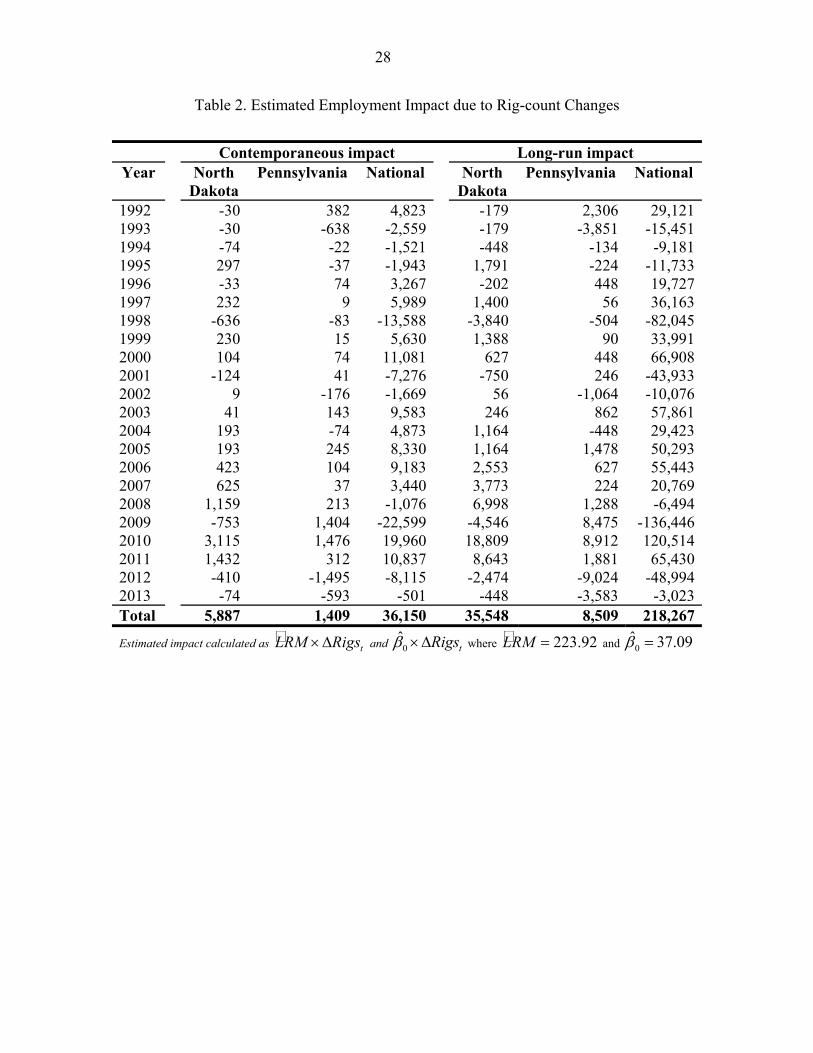
same month, and the LRM, 224 jobs in the long run.18 Figure 7 shows the IRF and CIRF, along with 95% confidence intervals for OLS, Multi-Clustered and Driscoll-Kraay serial and cross-sectional correlation consistent (SCC) errors. While the individual impulse responses themselves may not all be statistically significant at the 5% level, their sum is. The biggest employment increase is coincident with an increase in rig-counts, but months 1t and 8t through 10t also see sizeable impacts. There are many possible explanations for the delayed impact: subsequent infrastructure build-out, delayed labor supply responses and delay in increased consumption by owners of labor, capital and minerals are all reasonable. Table2 shows what the implied annual contemporaneous and long-run job-impacts would be from changes in rig-counts using estimates from model (2).19 As mentioned earlier, these estimates are much smaller than those obtained via I/O models. It is important to note that the long-run estimates are for the cumulative dynamic effects, which will be realized over a multi-year time horizon—not the year to which they correspond in the table. Furthermore, as documented in the new EIA Drilling Productivity Report, shale gas and tight oil production per new well has increased dramatically since 2007. 20 Thus, seemingly lower rig-counts do not correspond to lower production. Without more structure on our model or detail in our rig-counts, we are unable to account for these changes in productivity. Thus, it seems reasonable to view years such as 2009—which corresponds to a drop in national rig-counts and a resulting decrease of 136,446 jobs—with some caution.

18 Our baseline results for model (2) are listed in the “LAU” column of the bottom half of Table, which is a set of robustness checksTable. The 95% confidence interval is 120 to 328 jobs per rig-count using Driscoll—Kraay standard errors. The interval shrinks to approximately 171 to 277 jobs under clustered standard errors.

19 State estimates were calculated as /Dec

itt Jan

Rigs Pop

times 0̂ or LRM . National estimates used

/Dec

iti States t Jan

Rigs Pop

20 The EIA Drilling Productivity Report is available at http://www.eia.gov/petroleum/drilling/

18

Figure 7. IRF and CIRF for Panel Model

VII. FOUR ROBUSTNESS CHECKS

A. Lag Lengths

The first robustness check is to verify that multipliers do not vary greatly with lag-lengths. In addition to our base model, we estimate our baseline model with three different sets of lag-lengths. In the first set, we only include the contemporaneous and first lag of rig-counts and 12 lags of employment. In the second and third we include through lags 13 and 24, respectively, of both employment and rig-counts since these lag lengths corresponded to minima in the BIC. Plots of the IRFs and CIRFs are shown in Figure 8. When lags of rig-counts are truncated, the employment response is more muted, which suggests that much of the employment activity happens with a lag. As lags 11 to 13 and lags 11 to 24 are added, the shapes of the IRF and CIRF do not change much, but the size of the effect does grow. A substantial portion of the increase in the multiplier seems to be due to the inclusion of more positive rig-count coefficients since the

-0.005%

0.000%

0.005%

0.010%

0.00%

0.02%

0.04%

0.06%

0.08%

IRF

CIR

F

0 6 12 18 24

StandardErrors

SCC

OLS

Cluster

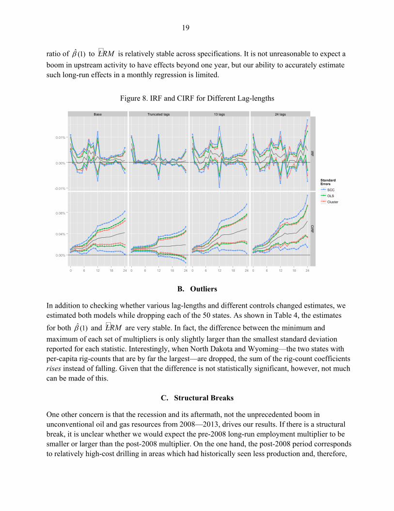
19

ratio of ˆ (1) to LRM is relatively stable across specifications. It is not unreasonable to expect a

boom in upstream activity to have effects beyond one year, but our ability to accurately estimate such long-run effects in a monthly regression is limited.

Figure 8. IRF and CIRF for Different Lag-lengths

B. Outliers

In addition to checking whether various lag-lengths and different controls changed estimates, we estimated both models while dropping each of the 50 states. As shown in Table 4, the estimates

for both ˆ (1) and LRM are very stable. In fact, the difference between the minimum and

maximum of each set of multipliers is only slightly larger than the smallest standard deviation reported for each statistic. Interestingly, when North Dakota and Wyoming—the two states with per-capita rig-counts that are by far the largest—are dropped, the sum of the rig-count coefficients rises instead of falling. Given that the difference is not statistically significant, however, not much can be made of this.

C. Structural Breaks

One other concern is that the recession and its aftermath, not the unprecedented boom in unconventional oil and gas resources from 2008—2013, drives our results. If there is a structural break, it is unclear whether we would expect the pre-2008 long-run employment multiplier to be smaller or larger than the post-2008 multiplier. On the one hand, the post-2008 period corresponds to relatively high-cost drilling in areas which had historically seen less production and, therefore,

Base Truncated lags 13 lags 24 lags

-0.01%

0.00%

0.01%

0.00%

0.04%

0.08%

IRF

CIR

F

0 6 12 18 24 0 6 12 18 24 0 6 12 18 24 0 6 12 18 24

StandardErrors

SCC

OLS

Cluster

20

would require more infrastructure investment to support drilling. On the other, firms drilling in these new areas might prefer to purchase inputs from areas like Texas and Louisiana with a historical oil and gas presence if these are cheaper or of higher quality. To examine this issue, we estimate the following model

( ) ) (t 2008)

( ) ) (t 2008

log( ) ( ) log( ) ( /

( / ( )) u

it it pre it

post it t ii t

L D JanEmp L Emp Rigs Pop

Rigs Pop D tL Jan

(3)

and test both that pre post as well as (1) (1)pre post using OLS, multi-way clustered and

Driscoll-Kraay estimates for the variance matrix. Under all three variance estimates, we reject both null hypotheses in favor of structural change at the 0.1% level. Post-2008 multipliers are more than twice as big as pre-2008 multipliers: 0.029% versus 0.066%. In the per-capita model, this translates to 143 versus 283 jobs per rig-count. 21 Figure 9 shows IRFs and CIRFs corresponding to the two periods, and it is clear that both are larger in the second period.

Figure 9. IRF and CIRF for Rig-Counts Pre and Post 2008

21 This outcome would also be consistent with the larger employment effects found in Hartley et al. (2013) where the wells drilled were all aimed at unconventional resources.

Pre-2008 Post-2008

-0.010%

-0.005%

0.000%

0.005%

0.010%

-0.025%

0.000%

0.025%

0.050%

0.075%

IRF

CIR

F

0 6 12 18 24 0 6 12 18 24

StandardErrors

SCC

OLS

Cluster

21

D. Population Scaling The choice of a population scaling variable does have implications for the magnitudes of the employment-multiplier, particularly in the per-capita model (2), which has a jobs-per-rig interpretation. The most problematic aspect of this scaling is that population growth, not just the variables of interest, affects results. First note the following equivalence: 1

1 1( / ) ( / ) .t t t t t tx z z x x z z

If the increase in employment per capita due to an increase in rig-counts per capita is simply

( / )tLRM Rigs Pop , then the resulting change in jobs can be decomposed as

1 1 1LR change in ( / )( ).t t t t tEmp LRM Rigs Pop Pop Emp LRM Rigs

In the log employment case, the problem is also present since the change in employment is computed as

1 1 1LR change in exp ( / ) ./t t t t t tEmp Emp LRM Rigs Pop LRM Rigs Pop Pop

While /LR

tEmp Rigs LRM , if long-run growth in jobs due to rigs is computed using rigs

per capita, the estimate will be “polluted” by population growth. To address this concern, we estimate equation (1) as well as (2), from which we take our job-creation multiplier, using a variety of different population scalings:

1. Working-age population as given in the Local Area Unemployment statistics from BLS, 2. Working-age population lagged by one month, which should be pre-determined with

respect to rig-counts, which might drive population movements in time t ,

3. Total population from the Current Population Survey, where months between June of each year are linearly interpolated,

4. Population in 1990 as given by the US Census, 5. Population in 2000 as given by the US Census and 6. Population in 2010 as given by the US Census.

The advantage of the last three population variables is that, with no population change, the “polluting” population growth term drops out of the estimation. When we use a fixed population parameter, model (2) is almost equivalent to weighted least squares (WLS). To see this, suppose that the variance of state’s idiosyncratic shock itu is proportional to the square of its population.

Then in OLS using first-differences of level variables, large states receive many times more weight than smaller states. If variables are all scaled by population, however, each state receives approximately the same weight in the model. Scaling by a constant population is not exactly

22

WLS since the common time-shock t is also implicitly divided by state population. Doing this,

however, makes sense since a common shock should induce a larger absolute employment change in larger states, and smaller absolute changes in smaller states. Estimation results of these robustness checks are available in Table5. The general result—that upstream drilling activity causes statistically significant increases in employment—holds true in all of the models, as does the pattern of dynamic response to rig-counts. Nevertheless, point estimates in the per-capita model are affected, with multipliers rising around 50% when population is held constant. Multipliers increase only about 20% in the log case—right around two standard deviations. From this we conclude that the LRMs calculated in our base model and our estimated employment impacts in Table2 are on the conservative side and could be up to 50% larger.

VIII. CONCLUSION To date, most estimates of the impact of unconventional oil and gas activity have been done through industry-related studies and using an Input-Output analysis. Analysis using a national-level VAR framework suggests that a ten percent increase in rig-counts raises employment in oil and gas extraction by approximately five percent after 24 months, but general employment impacts and employment impacts in manufacturing are not statistically distinguishable from zero. Using a dynamic panel model we confirm the hypothesis that increased drilling for oil and gas creates jobs, but we find the employment impacts to be much smaller than figures put forward by Input-Output studies. In particular, we estimate that the long-run employment impact of an additional rig-count per million people is an increase of 0.068% in total employment. A per-capita formulation of the model yields a LRM of 224 jobs per rig-count. Our estimates appear robust to autocorrelation, heteroskedasticity and cross-sectional dependency in the error terms. They also appear to be consistent across sets of states included in our sample and different lag-lengths. We find some evidence that upstream activity may have had a larger impact post-2008, though we cannot say as to why this would be. Additionally, using other measures of population increases our job-creation estimates by up to 50%. The fact that different modeling approaches result in substantially different estimates of the employment impacts suggests the need for further research in order to better understand the role of alternative modeling assumptions on these results.

23

REFERENCES

Arora, Vipin, and Jozef Lieskovsky, 2014, “Natural Gas and U.S. Economic Activity.” The Energy Journal 35 (3). doi:10.5547/01956574.35.3.8.

Black, Dan, Terra McKinnish, and Seth Sanders. 2005. “The Economic Impact Of The Coal Boom And Bust.” The Economic Journal 115 (503): 449–76.

Blanchard, Olivier Jean, and Lawrence F. Katz. 1992. “Regional Evolutions.” Brookings Papers on Economic Activity 1 (1992): 1–61.

Colin Cameron, A., J.B. Gelbach, and D.L. Miller. 2011. “Robust Inference with Multiway Clustering.” Journal of Business and Economic Statistics 29 (2): 238–49.

Considine, Timothy J., Robert Watson, and Seth Blumsack. 2010. The Economic Impacts of the Pennsylvania Marcellus Shale Natural Gas Play: An Update. Funded by Marcellus Shale Gas Coalition. http://marcelluscoalition.org/wp-content/uploads/2010/05/PA-Marcellus-Updated-Economic-Impacts-5.24.10.3.pdf.

Considine, Timothy, Robert Watson, Rebecca Entler, and Jeffrey Sparks. 2009. An Emerging Giant: Prospects and Economic Impacts of Developing the Marcellus Shale Natural Gas Play. http://marcelluscoalition.org/wp-content/uploads/2010/05/EconomicImpactsofDevelopingMarcellus.pdf.

Driscoll, John C., and Aart C. Kraay. 1998. “Consistent Covariance Matrix Estimation with Spatially Dependent Panel Data.” Review of Economics and Statistics 80 (4): 549–60.

Fetzer, Thiemo. 2014. “Fracking Growth”. Working paper. http://www.trfetzer.com/wp-content/uploads/fracking-local.pdf.

Han, Chirok, Peter CB Phillips, and Donggyu Sul. 2013. “Lag Length Selection in Panel Autoregression.” Yale University Department of Economics Working Pa-Pers. http://www.utdallas.edu/~d.sul/papers/BIC_ER_Final.pdf.

Hartley, Peter, Kenneth B. Medlock III, Ted Temzelides, and Xinya Zhang. 2013. Local Employment Impact from Competing Energy Sources: Shale Gas versus Wind Generation in Texas. Baker Institute for Public Policy, Rice University. http://www.owlnet.rice.edu/~tl5/jobs.pdf.

Higginbotham, Amy, Adam Pellillo, Tami Gurley-Calvez, and Tom S. Witt. 2010. The Economic Impact of the Natural Gas Industry and the Marcellus Shale Development in West Virginia in 2009. Prepared for West Virginia Oil and Natural Gas Association. http://www.be.wvu.edu/bber/pdfs/BBEr-2010-22.pdf.

24

Hooker, Mark A., and Michael M. Knetter. 1997. “The Effects of Military Spending on Economic Activity: Evidence from State Procurement Spending.” Journal of Money, Credit & Banking (Ohio State University Press) 29 (3): 400–421.

IHS Global Insight. 2011. The Economic and Employment Contributions of Shale Gas in the United States. Prepared for America’s Natural Gas Alliance. http://www.anga.us/media/content/F7D1441A-09A5-D06A-9EC93BBE46772E12/files/shale-gas-economic-impact-dec-2011.pdf.

Judson, Ruth A., and Ann L. Owen. 1999. “Estimating Dynamic Panel Data Models: A Guide for Macroeconomists.” Economics Letters 65 (1): 9–15.

Kinnaman, Thomas C. 2011. “The Economic Impact of Shale Gas Extraction: A Review of Existing Studies.” Ecological Economics 70 (7): 1243–49. doi:10.1016/j.ecolecon.2011.02.005.

Lütkepohl, Helmut. 2005. New Introduction to Multiple Time Series Analysis. New York: Springer.

Marchand, Joseph. 2012. “Local Labor Market Impacts of Energy Boom-Bust-Boom in Western Canada.” Journal of Urban Economics 71 (1): 165–74. doi:10.1016/j.jue.2011.06.001.

Murray, Sherry, and Teri Ooms. 2008. The Economic Impact of Marcellus Shale in Northeastern Pennsylvania. Joint Urban Studies Center. http://www.institutepa.org/PDF/Marcellus/mtwhitepaper.pdf.

Scott, Loren C. 2009. The Economic Impact of the Haynesville Shale on the Louisiana Economy in 2008. Loren C. Scott & Associates. http://dnr.louisiana.gov/assets/docs/mineral/haynesvilleshale/loren-scott-impact2008.pdf.

Swift, T. K., M. G. Moore, and E. Sanchez. 2011. Shale Gas and New Petrochemicals Investment: Benefits for the Economy, Jobs, and US Manufacturing. American Chemistry Council. http://chemistrytoenergy.com/sites/chemistrytoenergy.com/files/ACC-Shale-Report.pdf.

Weber, Jeremy G.. “A Decade of Natural Gas Development: The Makings of a Resource Curse?” Resource and Energy Economics 37: 168–83, forthcoming.

———. 2012. “The Effects of a Natural Gas Boom on Employment and Income in Colorado, Texas, and Wyoming.” Energy Economics 34 (5): 1580–88.

25

APPENDIX

A. National Data

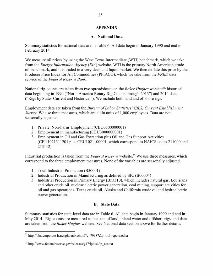
Summary statistics for national data are in Table 6. All data begin in January 1990 and end in February 2014. We measure oil prices by using the West Texas Intermediate (WTI) benchmark, which we take from the Energy Information Agency (EIA) website. WTI is the primary North American crude oil benchmark, and it is traded in a very deep and liquid market. We then deflate this price by the Producer Price Index for All Commodities (PPIACO), which we take from the FRED data service of the Federal Reserve Bank. National rig-counts are taken from two spreadsheets on the Baker Hughes website22: historical data beginning in 1990 (“North America Rotary Rig Counts through 2013”) and 2014 data (“Rigs by State- Current and Historical”). We include both land and offshore rigs. Employment data are taken from the Bureau of Labor Statistics’ (BLS) Current Establishment Survey. We use three measures, which are all in units of 1,000 employees. Data are not seasonally adjusted.

1. Private, Non-Farm Employment (CEU0500000001) 2. Employment in manufacturing (CEU3000000001) 3. Employment in Oil and Gas Extraction plus Oil and Gas Support Activities

(CEU1021311201 plus CEU1021100001, which correspond to NAICS codes 211000 and 213112)

Industrial production is taken from the Federal Reserve website.23 We use three measures, which correspond to the three employment measures. None of the variables are seasonally adjusted.

1. Total Industrial Production (B50001) 2. Industrial Production in Manufacturing as defined by SIC (B00004) 3. Industrial Production in Primary Energy (B53310), which includes natural gas, Louisiana

and other crude oil, nuclear electric power generation, coal mining, support activities for oil and gas operations, Texas crude oil, Alaska and California crude oil and hydroelectric power generation.

B. State Data Summary statistics for state-level data are in Table 6. All data begin in January 1990 and end in May 2014. Rig-counts are measured as the sum of land, inland water and offshore rigs, and data are taken from the Baker Hughes website. See National data section above for further details.

22 http://phx.corporate-ir.net/phoenix.zhtml?c=79687&p=irol-reportsother

23 http://www.federalreserve.gov/releases/g17/ipdisk/ip_nsa.txt

26

Employment data are taken from the BLS Current Establishment Survey State and Metro dataset. As in the national case, we use Private, Non-Farm Employment, which is not seasonally adjusted and measured in thousands. We work with a variety of population measures. Our primary measure of population is the BLS Local Area Unemployment (LAU) Statistics series “Civilian noninstitutional population.” As defined by the BLS, this panel captures the population of 16 years of age or older who are not institutionalized or in the armed services.24 Our other population measure is the Census Bureau’s midyear population estimate, and we download it from the “Annual State Personal Income and Employment” tables on the Bureau of Economic Analysis website.25 We prefer the “Civilian noninstitutional population” measure to the Census estimate since the former is reported on a monthly basis, whereas the latter is reported annually.

24 See http://www.bls.gov/lau/rdscnp16.htm for the exact definition.

25 http://www.bea.gov/iTable/iTable.cfm?ReqID=9&step=1#reqid=9&step=1&isuri=1

27

Table1. Base Model with Different Standard Errors

Estimate (%) OLS Cluster SCC

, 1log i tEmployment -3.9837 (0.8600)***

(3.9997) (2.2742)

, 2log i tEmployment 1.4725 (0.8580) (2.0487) (1.6136)

, 3log i tEmployment 5.2474 (0.8563)***

(1.9485)**

(1.4385)***

, 4log i tEmployment -0.0126 (0.8569) (1.4903) (1.3907)

, 5log i tEmployment -0.6589 (0.8577) (2.0285) (1.0915)

, 6log i tEmployment 2.8201 (0.8564)***

(2.5640) (1.2659)*

, 7log i tEmployment 3.4738 (0.8536)***

(2.2193) (1.1474)**

, 8log i tEmployment 0.5007 (0.8551) (1.8788) (1.2442)

, 9log i tEmployment 3.5216 (0.8529)***

(1.7197)* (1.1881)

**

, 10log i tEmployment 2.9141 (0.8471)***

(1.5783) (1.2484)*

, 11log i tEmployment 7.9422 (0.8452)***

(2.5955)**

(1.7775)***

, 12log i tEmployment 25.3623 (0.8445)***

(4.4197)***

(2.6803)***

,/ i tRigs Pop 0.0077 (0.0012)***

(0.0015)***

(0.0016)***

, 1/ i tRigs Pop 0.0033 (0.0012)**

(0.0012)**

(0.0014)*

, 2/ i tRigs Pop 0.0017 (0.0012) (0.0012) (0.0017)

, 3/ i tRigs Pop -0.0007 (0.0012) (0.0013) (0.0019)

, 4/ i tRigs Pop -0.0005 (0.0012) (0.0015) (0.0022)

, 5/ i tRigs Pop 0.0001 (0.0012) (0.0016) (0.0017)

, 6/ i tRigs Pop 0.0020 (0.0012) (0.0022) (0.0016)

, 7/ i tRigs Pop 0.0009 (0.0012) (0.0020) (0.0019)

, 8/ i tRigs Pop 0.0048 (0.0012)***

(0.0015)**

(0.0019)*

, 9/ i tRigs Pop 0.0030 (0.0012)* (0.0011)

** (0.0016)

, 10/ i tRigs Pop 0.0039 (0.0012)**

(0.0011)***

(0.0016)*

ˆ (1) 0.0261 (0.0034)***

(0.0032)***

(0.0034) ***

LRM 0.0508 (0.0069)***

(0.0089)***

(0.0069) ***

Estimates and standard errors are scaled by 100 to represent approximate percentage points. ***

p < 0.001, **

p < 0.01, *p < 0.05. Standard errors in parenthesis.

50 states, 268 months, 13,400 observations. State-month and time FE included.

28

Table 2. Estimated Employment Impact due to Rig-count Changes

Contemporaneous impact Long-run impact

Year North Dakota

Pennsylvania National North Dakota

Pennsylvania National

1992 -30 382 4,823 -179 2,306 29,121 1993 -30 -638 -2,559 -179 -3,851 -15,451 1994 -74 -22 -1,521 -448 -134 -9,181 1995 297 -37 -1,943 1,791 -224 -11,733 1996 -33 74 3,267 -202 448 19,727 1997 232 9 5,989 1,400 56 36,163 1998 -636 -83 -13,588 -3,840 -504 -82,045 1999 230 15 5,630 1,388 90 33,991 2000 104 74 11,081 627 448 66,908 2001 -124 41 -7,276 -750 246 -43,933 2002 9 -176 -1,669 56 -1,064 -10,076 2003 41 143 9,583 246 862 57,861 2004 193 -74 4,873 1,164 -448 29,423 2005 193 245 8,330 1,164 1,478 50,293 2006 423 104 9,183 2,553 627 55,443 2007 625 37 3,440 3,773 224 20,769 2008 1,159 213 -1,076 6,998 1,288 -6,494 2009 -753 1,404 -22,599 -4,546 8,475 -136,446 2010 3,115 1,476 19,960 18,809 8,912 120,514 2011 1,432 312 10,837 8,643 1,881 65,430 2012 -410 -1,495 -8,115 -2,474 -9,024 -48,994 2013 -74 -593 -501 -448 -3,583 -3,023 Total 5,887 1,409 36,150 35,548 8,509 218,267

Estimated impact calculated as tLRM Rigs and 0ˆ

tRigs where 223.92LRM and 0ˆ 37.09

29

Table 3. Different Lag Lengths

Base Truncated lags 13 lags 24 lags

, 0/ i tRigs Pop 0.0077 (0.0016)***

0.0076 (0.0017)***

0.0077 (0.0016)***

0.0076 (0.0016)***

, 1/ i tRigs Pop 0.0033 (0.0014)* 0.0034 (0.0015)

* 0.0033 (0.0014)

* 0.0031 (0.0013)

*

, 2/ i tRigs Pop 0.0017 (0.0017) 0.0017 (0.0017) 0.0019 (0.0016)

, 3/ i tRigs Pop -0.0007 (0.0019) -0.0008 (0.0019) -0.0004 (0.0018)

, 4/ i tRigs Pop -0.0005 (0.0022) -0.0003 (0.0021) 0.0002 (0.0021)

, 5/ i tRigs Pop 0.0001 (0.0017) 0.0005 (0.0016) 0.0008 (0.0015)

, 6/ i tRigs Pop 0.0020 (0.0016) 0.0021 (0.0017) 0.0021 (0.0015)

, 7/ i tRigs Pop 0.0009 (0.0019) 0.0015 (0.0019) 0.0019 (0.0019)

, 8/ i tRigs Pop 0.0048 (0.0019)* 0.0047 (0.0020)

* 0.0053 (0.0018)

**

, 9/ i tRigs Pop 0.0030 (0.0016) 0.0032 (0.0016)* 0.0029 (0.0016)

, 10/ i tRigs Pop 0.0039 (0.0016)* 0.0033 (0.0017)

* 0.0032 (0.0016)

*

, 11/ i tRigs Pop 0.0023 (0.0017) 0.0018 (0.0016)

, 12/ i tRigs Pop 0.0000 (0.0015) -0.0001 (0.0016)

, 13/ i tRigs Pop 0.0026 (0.0017) 0.0015 (0.0017)

, 14/ i tRigs Pop 0.0026 (0.0016)

, 15/ i tRigs Pop -0.0024 (0.0016)

, 16/ i tRigs Pop 0.0002 (0.0015)

, 17/ i tRigs Pop -0.0001 (0.0015)

, 18/ i tRigs Pop 0.0001 (0.0015)

, 19/ i tRigs Pop -0.0012 (0.0019)

, 20/ i tRigs Pop 0.0010 (0.0016)

, 21/ i tRigs Pop 0.0039 (0.0018)*

, 22/ i tRigs Pop 0.0019 (0.0017)

, 23/ i tRigs Pop 0.0055 (0.0015)***

, 24/ i tRigs Pop 0.0034 (0.0018)

ˆ (1) 0.0261 (0.0034)***

0.0110 (0.0015)***

0.0317 (0.0038)***

0.0467 (0.0054)***

LRM 0.0508 (0.0069)***

0.0219 (0.0033)***

0.0631 (0.0080)***

0.0924 (0.0115)***

Estimates and standard errors scaled by 100 to represent approximate percentage changes. ***

p < 0.001, **

p < 0.01, *p < 0.05. Driscoll-Kraay standard errors in parenthesis. 12, 12, 13 and 24 lags of employment as well

as state-month and time FE included. 50 states, 268 months, 13,400 observations.

30

Table 4. Multipliers for Model (1) When Each State is Omitted

Alabama Alaska Arizona Arkansas California Colorado Connecticut Delaware Florida Georgia

ˆ(1) 0.0260 0.0253 0.0263 0.0260 0.0263 0.0261 0.0262 0.0260 0.0263 0.0260

(1)ˆ (0.0034) (0.0033) (0.0034) (0.0034) (0.0034) (0.0034) (0.0034) (0.0033) (0.0034) (0.0034)

LRM 0.0508 0.0498 0.0491 0.0509 0.0503 0.0503 0.0510 0.0522 0.0502 0.0507

ˆLRM (0.0070) (0.0068) (0.0066) (0.0070) (0.0068) (0.0069) (0.0069) (0.0071) (0.0068) (0.0069)

Hawaii Idaho Illinois Indiana Iowa Kansas Kentucky Louisiana Maine Maryland

ˆ(1) 0.0261 0.0263 0.0262 0.0260 0.0261 0.0264 0.0259 0.0271 0.0257 0.0260

(1)ˆ (0.0034) (0.0034) (0.0034) (0.0034) (0.0034) (0.0034) (0.0034) (0.0033) (0.0034) (0.0034)

LRM 0.0490 0.0510 0.0512 0.0506 0.0509 0.0515 0.0508 0.0567 0.0506 0.0509

ˆLRM (0.0066) (0.0069) (0.0070) (0.0069) (0.0070) (0.0070) (0.0070) (0.0073) (0.0070) (0.0070)

Massachusetts Michigan Minnesota Mississippi Missouri Montana Nebraska Nevada New Hampshire New Jersey

ˆ(1) 0.0259 0.0258 0.0261 0.0263 0.0260 0.0263 0.0262 0.0268 0.0260 0.0260

(1)ˆ (0.0034) (0.0034) (0.0034) (0.0034) (0.0034) (0.0034) (0.0034) (0.0034) (0.0034) (0.0034)

LRM 0.0502 0.0502 0.0510 0.0514 0.0509 0.0518 0.0515 0.0485 0.0510 0.0507

ˆLRM (0.0069) (0.0069) (0.0070) (0.0069) (0.0070) (0.0070) (0.0070) (0.0064) (0.0070) (0.0070)

New Mexico New York North Carolina North Dakota Ohio Oklahoma Oregon Pennsylvania Rhode Island South Carolina

ˆ(1) 0.0261 0.0260 0.0261 0.0259 0.0261 0.0253 0.0261 0.0260 0.0257 0.0259

(1)ˆ (0.0034) (0.0034) (0.0034) (0.0043) (0.0034) (0.0035) (0.0034) (0.0034) (0.0034) (0.0034)

LRM 0.0504 0.0501 0.0509 0.0498 0.0508 0.0494 0.0505 0.0504 0.0502 0.0508

ˆLRM (0.0070) (0.0069) (0.0070) (0.0087) (0.0070) (0.0070) (0.0069) (0.0069) (0.0069) (0.0070)

South Dakota Tennessee Texas Utah Vermont Virginia Washington West Virginia Wisconsin Wyoming

ˆ(1) 0.0260 0.0260 0.0255 0.0260 0.0256 0.0261 0.0262 0.0265 0.0261 0.0287

(1)ˆ (0.0034) (0.0034) (0.0034) (0.0034) (0.0033) (0.0034) (0.0034) (0.0034) (0.0034) (0.0043)

LRM 0.0508 0.0506 0.0493 0.0496 0.0507 0.0508 0.0510 0.0518 0.0509 0.0560

ˆLRM (0.0070) (0.0069) (0.0069) (0.0068) (0.0070) (0.0070) (0.0069) (0.0070) (0.0070) (0.0087)

Estimates and standard errors scaled by 100 to represent approximate percentage changes. OLS standard errors in parenthesis. 49 states, 268 months, 13,132 observations.

31

Table 5. Per-capita and Log Models with Different Population Scaling

Log employment models (units are percentages)

LAU Lag LAU CPS Interpolated CPS 1990 CPS 2000 CPS 2010

,/ i tRigs Pop 0.008 (0.002)***

0.008 (0.002)***

0.011 (0.002)***

0.010 (0.002)***

0.011 (0.002)***

0.012 (0.003)***

, 1/ i tRigs Pop 0.003 (0.001)* 0.003 (0.001)

* 0.004 (0.002)

* 0.004 (0.002)

* 0.004 (0.002)

* 0.005 (0.002)

*

, 2/ i tRigs Pop 0.002 (0.002) 0.002 (0.002) 0.002 (0.002) 0.002 (0.002) 0.003 (0.002) 0.003 (0.002)

, 3/ i tRigs Pop -0.001 (0.002) -0.001 (0.002) -0.001 (0.003) -0.001 (0.002) -0.001 (0.003) -0.001 (0.003)

, 4/ i tRigs Pop -0.001 (0.002) -0.001 (0.002) -0.001 (0.003) 0.000 (0.003) 0.000 (0.003) 0.000 (0.003)

, 5/ i tRigs Pop 0.000 (0.002) 0.000 (0.002) 0.000 (0.002) 0.000 (0.002) 0.000 (0.002) 0.000 (0.002)

, 6/ i tRigs Pop 0.002 (0.002) 0.002 (0.002) 0.003 (0.002) 0.003 (0.002) 0.003 (0.002) 0.003 (0.002)

, 7/ i tRigs Pop 0.001 (0.002) 0.001 (0.002) 0.001 (0.003) 0.001 (0.002) 0.001 (0.003) 0.001 (0.003)

, 8/ i tRigs Pop 0.005 (0.002)* 0.005 (0.002)

* 0.006 (0.003)

* 0.006 (0.002)

* 0.006 (0.003)

* 0.006 (0.003)

*

, 9/ i tRigs Pop 0.003 (0.002) 0.003 (0.002) 0.004 (0.002) 0.003 (0.002) 0.004 (0.002) 0.004 (0.002)

, 10/ i tRigs Pop 0.004 (0.002)* 0.004 (0.002)

* 0.005 (0.002)

* 0.005 (0.002)

* 0.005 (0.002)

* 0.006 (0.002)

*

ˆ (1) 0.008 (0.002)***

0.008 (0.002)***

0.011 (0.002)***

0.010 (0.002)***

0.011 (0.002)***

0.012 (0.003)***

LRM 0.003 (0.001)* 0.003 (0.001)

* 0.004 (0.002)

* 0.004 (0.002)

* 0.004 (0.002)

* 0.005 (0.002)

*

Employment per capita models (units are jobs) LAU Lag LAU CPS Interpolated CPS 1990 CPS 2000 CPS 2010

,/ i tRigs Pop 37.09 (8.15)***

41.62 (8.71)***

36.69 (8.43)***

32.88 (8.75)***

34.41 (8.74)***

34.23 (8.74)***

, 1/ i tRigs Pop 13.60 (8.01) 15.39 (7.54)* 15.52 (7.08)

* 11.00 (7.04) 11.60 (7.11) 12.20 (7.12)

, 2/ i tRigs Pop 8.48 (9.77) 10.21 (9.19) 12.73 (7.69) 10.22 (8.06) 12.46 (8.07) 12.03 (8.09)

, 3/ i tRigs Pop 2.45 (9.43) -3.14 (11.37) 1.75 (8.10) 0.73 (7.51) 3.90 (7.78) 4.53 (7.97)

, 4/ i tRigs Pop 2.39 (9.78) 5.92 (10.56) 6.79 (8.97) 12.18 (8.63) 12.78 (8.64) 13.21 (8.63)

, 5/ i tRigs Pop -0.68 (7.54) -0.61 (9.02) 3.11 (7.53) 5.68 (7.75) 7.76 (7.68) 9.51 (7.92)

, 6/ i tRigs Pop 9.15 (9.01) 8.38 (7.86) 10.89 (7.75) 14.07 (7.37) 14.27 (7.53) 13.31 (7.60)

, 7/ i tRigs Pop 7.10 (7.85) 3.09 (10.04) 4.31 (8.48) 4.64 (8.82) 5.07 (8.91) 6.10 (9.35)

, 8/ i tRigs Pop 23.31 (8.69)**

26.45 (8.94)**

22.47 (8.67)**

22.99 (8.34)**

22.56 (8.42)**

22.41 (8.45)**

, 9/ i tRigs Pop 15.81 (7.65)* 15.53 (7.56)

* 13.23 (7.23) 10.40 (7.71) 11.78 (7.81) 13.05 (7.96)

, 10/ i tRigs Pop 22.95 (8.58)**

21.08 (7.93)**

19.89 (7.35)**

17.52 (7.07)* 18.52 (7.06)

** 18.93 (7.12)

**

ˆ (1) 141.66 (16.56)***

143.92 (17.12)***

147.38 (16.20)***

142.31 (17.48)***

155.11 (16.08)***

159.50 (16.06)***

LRM 223.92 (27.48)***

219.82 (27.37)***

223.79 (25.67)***

388.53 (51.48)***

334.96 (37.56)***

309.08 (33.46)***

***

p < 0.001, **

p < 0.01, *p < 0.05. Driscoll-Kraay standard errors in parenthesis. Log employment estimates are percentage terms.

50 states, 268 months, 13,400 observations. State-month and time FE included, as well as lags 1 to 12 of employment variable.

32

Table 6. Summary Statistics

National variables Obs N T Start End Mean Std. Dev. Min Max

log( / )WTI PPIACO 290 1 290 1990m1 2014m2 -1.396 0.482 -2.381 -0.404log( )Rig count 290 1 290 1990m1 2014m2 6.997 0.369 6.207 7.609log(Total IP) 290 1 290 1990m1 2014m2 4.427 0.161 4.093 4.628log(IP in Mfg - SIC) 290 1 290 1990m1 2014m2 4.398 0.176 4.025 4.635log(IP in Primary Energy) 290 1 290 1990m1 2014m2 4.637 0.055 4.476 4.839log(Total Employment) 290 1 290 1990m1 2014m2 11.565 0.083 11.385 11.669log(Employment in Mfg) 290 1 290 1990m1 2014m2 9.616 0.151 9.336 9.791log(Employmentin O&G Extraction) 290 1 290 1990m1 2014m2 5.692 0.225 5.401 6.233

State variables Obs N T Start End Mean Std. Dev. Min Max

CPS Population (millions) 1,150 50 23 1990m1 2014m5 5.661 6.223 0.454 38.041Lin. Interp. CPS Population (millions) 14,650 50 293 1990m1 2014m5 5.702 6.274 0.454 38.727LAU Working-age population (millions) 14,650 50 293 1990m1 2014m5 4.336 4.745 0.329 29.955Rig-count 14,650 50 293 1990m1 2014m5 23.544 82.207 0.000 946.000Rig-count per capita (LAU pop, millions) 14,650 50 293 1990m1 2014m5 9.746 28.658 0.000 367.323CES Employment (thousands, NSA) 14,650 50 293 1990m1 2014m5 2,101.435 2,218.420 131.600 13,062.500

33

Figure 10. Map of US Shale Gas and Tight Oil Plays

34

Figure 11. Rig-counts Per Million Working-age People

Alabama Alaska Arizona Arkansas California

Colorado Connecticut Delaware Florida Georgia

Hawaii Idaho Illinois Indiana Iowa

Kansas Kentucky Louisiana Maine Maryland

Massachusetts Michigan Minnesota Mississippi Missouri

Montana Nebraska Nevada New Hampshire New Jersey

New Mexico New York North Carolina North Dakota Ohio

Oklahoma Oregon Pennsylvania Rhode Island South Carolina

South Dakota Tennessee Texas Utah Vermont

Virginia Washington West Virginia Wisconsin Wyoming

0.0

2.5

5.0

7.5

10.0

12.5

10

20

30

40

0.00

0.050.10

0.15

0.200.25

0

10

20

0.5

1.0

1.5

2.0

2.5

10

20

30

-0.50

-0.25

0.00

0.25

0.50

-0.50

-0.25

0.00

0.25

0.50

0.0

0.1

0.2

0.3

0.00

0.05

0.10

0.15

0.00.51.0

1.52.0

2.5

0.00

0.25

0.50

0.75

0.0

0.2

0.4

0.6

0.0

0.5

1.0

0.00

0.05

0.10

0.15

0.20

0

10

20

30

0

1

2

3

4

30

40

50

60

70

0.0

0.1

0.2

0.00

0.05

0.10

0.15

0.20

-0.50

-0.25

0.00

0.25

0.50

0

1

2

3

-0.50

-0.25

0.00

0.25

0.50

2.5

5.0

7.5

-0.50

-0.25

0.00

0.25

0.50

0

10

20

30

0

1

2

3

0

2

4

6

-0.50

-0.25

0.00

0.25

0.50

0.00

0.01

0.02

0.03

203040506070

0.0

0.2

0.4

0.6

0.00

0.01

0.02

0.03

0.04

0.05

0

100

200

300

1

2

3

4

20

40

60

0.0

0.2

0.4

0.6

0.8

0

3

6

9

-0.50

-0.25

0.00

0.25

0.50

-0.50

-0.25

0.00

0.25

0.50

0

2

4

6

0.0

0.4

0.8

1.2

20

30

40

50

5

10

15

20

25

0.0

0.5

1.0

1.5

2.0

0.0

0.5

1.0

0.0

0.1

0.2

0.3

0.4

5

10

15

20

25

0.0

0.1

0.2

100

200

1990

1995

2000

2005

2010

2015

1990

1995

2000

2005

2010

2015

1990

1995

2000

2005

2010

2015

1990

1995

2000

2005

2010

2015

1990

1995

2000

2005

2010

2015

35

35

Figure 12. Rig-counts (levels)

Alabama Alaska Arizona Arkansas California

Colorado Connecticut Delaware Florida Georgia

Hawaii Idaho Illinois Indiana Iowa

Kansas Kentucky Louisiana Maine Maryland

Massachusetts Michigan Minnesota Mississippi Missouri

Montana Nebraska Nevada New Hampshire New Jersey

New Mexico New York North Carolina North Dakota Ohio

Oklahoma Oregon Pennsylvania Rhode Island South Carolina

South Dakota Tennessee Texas Utah Vermont

Virginia Washington West Virginia Wisconsin Wyoming

0

10

20

30

4

8

12

16

0.00

0.25

0.50

0.75

1.00

0

20

40

60

10

20

30

40

50

25

50

75

100

125

-0.50

-0.25

0.00

0.25

0.50

-0.50

-0.25

0.00

0.25

0.50

0

1

2

3

0.00

0.25

0.50

0.75

1.00

0.0

0.5

1.0

1.5

2.0

0.00

0.25

0.50

0.75

1.00

0

2

4

6

0

2

4

6

0.0

0.1

0.2

0.3

0.4

0

20

40

60

0

4

8

12

100

150

200

0.000.050.10

0.150.200.25

0.00

0.25

0.50

0.75

1.00

-0.50

-0.25

0.00

0.25

0.50

0

5

10

15

20

-0.50

-0.25

0.00

0.25

0.50

5

10

15

20

-0.50

-0.25

0.00

0.25

0.50

0

10

20

0

1

2

3

0

2

4

6

-0.50

-0.25

0.00

0.25

0.50

0.00

0.05

0.10

0.15

0.20

20

40

60

80

100

0

3

6

9

0.00

0.050.100.150.20

0.25

0

50

100

150

200

10

20

30

40

50

100

150

200

0.0

0.5

1.0

1.5

2.0

0

30

60

90

120

-0.50

-0.25

0.00

0.25

0.50

-0.50

-0.25

0.00

0.25

0.50

0

1

2

3

4

0

2

4

6

250

500

750

10

20

30

40

50

0.00

0.25

0.50

0.75

1.00

0

2

4

6

0.0

0.5

1.0

1.5

2.0

10

20

30

0.00

0.25

0.50

0.75

1.00

30

60

90

1990

1995

2000

2005

2010

2015

1990

1995

2000

2005

2010

2015

1990

1995

2000

2005

2010

2015

1990

1995

2000

2005

2010

2015

1990

1995

2000

2005

2010

2015