University of Rhode IslandDigitalCommons@URI

Human Development and Family Studies FacultyPublications Human Development and Family Studies

2019

Employment Type, Residential Status, andConsumer Financial Capability: Evidence fromChina Household Finance SurveyXu CuiUniversity of Rhode Island

Jing Jian XiaoUniversity of Rhode Island, jjxiao@uri.edu

See next page for additional authors

Follow this and additional works at: https://digitalcommons.uri.edu/hdf_facpubs

The University of Rhode Island Faculty have made this article openly available.Please let us know how Open Access to this research benefits you.

This is a pre-publication author manuscript of the final, published article.

Terms of UseThis article is made available under the terms and conditions applicable towards Open Access PolicyArticles, as set forth in our Terms of Use.

This Article is brought to you for free and open access by the Human Development and Family Studies at DigitalCommons@URI. It has been acceptedfor inclusion in Human Development and Family Studies Faculty Publications by an authorized administrator of DigitalCommons@URI. For moreinformation, please contact digitalcommons@etal.uri.edu.

Citation/Publisher AttributionCui, Xu, et al. "Employment Type, Residential Status, and Consumer Financial Capability: Evidence from China Household FinanceSurvey." The Singapore Economic Review, vol. 64, no. 1, 2019, pp. 57-81. doi: 10.1142/S0217590817430032Available at: https://doi.org/10.1142/S0217590817430032

AuthorsXu Cui, Jing Jian Xiao, and Jingtao Yi

This article is available at DigitalCommons@URI: https://digitalcommons.uri.edu/hdf_facpubs/44

Employment Type, Residential Status, and Consumer Financial

Capability: Evidence from China Household Finance Survey Xu Cui

School of Business

Renmin University of China

Department of Human Development and Family Studies

University of Rhode Island

billcui_work@ruc.edu.cn Jing Jian Xiao

Department of Human Development and Family Studies

University of Rhode Island

jjxiao@uri.edu

Jingtao Yia School of Business

Renmin University of China

yijingtao@rbs.ruc.edu.cn

Abstract

Research on consumer financial capability is important for consumer financial wellbeing and

emerging in the literature. However, studies on consumer financial capability in the Chinese

context remain limited. To fill up the research gap, we used data from the 2011 China

Household Finance Survey to investigate whether employment type and residential status

were associated with consumer financial capability in China. Consumer financial capability

was measured by the range of financial assets. Results from OLS and Poisson regressions

showed that people employed in the government-managed system, with urban residence

registration, and with non-local rural residence registration had a better financial capability

than their respective counterparts. The results have policy implications for improving

consumer financial education and supporting vulnerable consumers.

a Corresponding author.

2

Keyword: China Household Finance Survey, Financial Capability, The Government-managed

System, Household Residence Registration

JEL Classifications: D140 R230

3

1 Introduction

Consumer financial capability refers to individual ability to apply appropriate financial

knowledge and perform desirable financial behavior to achieve financial wellbeing

(Atkinson et al. 2006; Lusardi and Mitchell, 2014; Xiao et al. 2014). Social movements

promoting financial capability started first in developed countries (Lusardi and Mitchell,

2011; OECD, 2016) and then occurred in developing countries. In China, the People’s Bank

of China launched the Financial Literacy Promotion Program in 2013 and set September

as the Financial Literacy Month every year (The Peoples’ Bank of China, 2013). The

program has made a call for research on consumer financial capability in China. Yin et al.

(2014) found that the proportion of Chinese who correctly answered financial literacy

questions was very low, with no more than 30% for each question. In comparison,

consumers in the U.S. (Lusardi and Mitchell, 2011) and European countries (OECD, 2016)

on average have better financial literacy levels than Chinese consumers, which implies

Chinese consumers need more financial education and protection. The purpose of this

study is to examine factors associated with consumer financial capability measured by the

household financial asset range using data from a large sample in China.

Research on consumer financial capability in China is limited mainly because of lack of

data. The China Household Financial Survey (CHFS) has provided opportunities for

researchers to study this topic with Chinese data. To our knowledge, research on financial

capability with the CHFS data is limited. This study contributes to the research literature

by examining factors associated with financial capability from the perspective of

background risks in China and focusing on two independent variables that have unique

4

Chinese features, the employment type and residence registration status. 2 In China,

people are employed in two major labor markets, the state-owned units and non-state-

owned units (National Bureau of Statistics of China, 2016). The state-owned unit is a

government-managed system including positions in civil service, public institutions, the

military, and state-owned enterprises. The non-state-owned unit is a non-government

managed system, such as collective and private-owned enterprises. Two systems have

major differences in terms of job security, income stability, and work related benefits. We

would like to examine if there are differences in financial capability between people

working in these two types of systems.

The other unique independent variable is the household residency registration status

(hukou) (National People's Congress of the People's Republic of China, 1958). In China,

people living in rural and urban areas are recorded in two different household residence

registration systems. People with urban and rural household registrations receive

different treatments in terms of job and life opportunities and benefits. In addition,

people with local and non-local household registrations receive differential treatments of

job and life opportunities and benefits. In this study, we would like to see if there are any

differences in financial capability between people with urban and rural household

registrations and with local and non-local household registrations.

2 Although there are other perspectives besides background risks, such as financial knowledge, skills and habits, since

they are not the focus of this study, we included these variables in the model as control variables, which are having an

undergraduate degree or higher, working in the financial service sectors, using credit cards, different preferences of

risks, and the preference for future vs. current consumption.

5

We found employees in the government-managed working system and people with

urban residence registration, who represented groups with low background risks, had

better financial capability. Among people with rural registrations, non-local people had

better financial capability than their local counterparts. As for controlled factors, we found

consumers with young age, having low income, without undergraduate or higher degree,

not using a credit card, working in non-financial service occupations, and living in the

northeast region tended to have a lower level of financial capability. Our findings provide

useful information for consumer policy makers and educators to identify vulnerable

consumers in terms of financial capability and deliver pertinent financial education to

them.

The remainder of this paper is organized as follows: section 2 presents literature

reviews and hypotheses, section 3 introduces the method including data description and

analysis strategy, section 4 presents the results, section 5 provides the robustness checks,

and section 6 concludes.

2 Literature Review and Hypotheses

2.1. Defining Financial Capability

Financial capability is defined differently in the research literature. Financial capability is

a multidimensional concept that examines individual ability from various angles such as

knowledge, habits, statuses, and access (Lin et al., 2016). Financial literacy is one main

area of financial capability (Lusardi and Mitchell, 2011). Abreu and Mendes (2010) defined

financial literacy as specific financial knowledge, the investors’ educational level, and the

sources of information commonly used by investors as the basis for their financial choices.

6

Lusardi and Mitchell (2014) used term “financial literacy” to represent individual ability to

process economic information and make informed decisions about financial planning,

wealth accumulation, debt, and pensions. Some scholars preferred to include more

dimensions to measure financial capability. Atkinson et al. (2006) used a set of financial

behaviors and a set of applied financial literacy questions called a “money quiz” to

measure financial capability. Taylor (2011) defined financial capability as people’s

knowledge of financial matters, their ability to manage their money and to take control of

their finances. His financial capability indicator was composed of measures of financial

behaviors and statuses. Xiao et al. (2014; 2015) defined consumer financial capability as

applying financial knowledge and engaging in desirable financial behavior to achieve

financial wellbeing. Previous research suggested that financial capability should include

three elements: financial literacy, financial behavior, and financial status.

Unlike previous studies that used multiple measures for financial capability, we used

the household financial asset range to measure financial capability. We believed this

measure was unique and a good proxy as it measured financial capability from all three

perspectives: financial literacy, financial behavior, and financial status. This unique

measure was supported by previous research.

First, a broader household financial asset range indicates a more sophisticated

financial literary. To build a more diversified portfolio of investment, more comprehensive

financial knowledge is needed, as shown by researchers who found positive correlations

between financial literacy and portfolio diversification (Guiso and Jappelli, 2008; Abreu

and Mendes, 2010), stock-market participation (Georgarakos and Inderst, 2011; van Rooij

7

et al., 2011) and risky asset share conditional on participation (Jappelli and Padula, 2015).

This is consistent with Robb and Woodyard (2011) where they found financial knowledge

and best practice behavior were highly correlated.

Second, holding a broad financial asset range is a desirable financial behavior. Based

on the portfolio diversification theory developed by Markowitz (1952), economic theories

and finance curriculums encourage people to hold a well-diversified portfolio for a best

mean return and variance combination. In the investment theory, investment

diversification is the rule of thumb to minimize one’s risk (Deidda, 2014). We believe

holding a broad household financial asset range is a desirable financial behavior.

Third, financial status is positively correlated with portfolio diversification. Tsigos and

Daly (2016) found risk tolerance increases significantly with wealth. Wealthier people tend

to invest more on risky assets (Cardak and Wilkins, 2009) and have more diversified

financial portfolio. In summary, research indicates that consumers with more

sophisticated financial capability tend to have a broader household financial asset range.

The two alternative variables that might be used to measure financial capability are

the share of financially risky assets in the total portfolio and the market value of financially

risky assets (see Yin et al., 2014). However, we chose not to use them because the

household financial asset range measure has several advantages over them. First, the

market value of each financially risky asset usually fluctuated every business day, which

creates difficulties for comparison at different interview dates. The survey lasted for more

than eight months. The values over such a long period of time might not be comparable.

Second, the market value of financially risky asset owned by interviewees was either an

8

approximation or was provided in ranges in the data. Interviewees might have difficulty

remembering the amount of their financially risky assets if they owned several types.

Third, the interviewees might not want to give true information about the amount of their

assets. The household financial asset range does not rely on this data to the same extent.

The household financial asset range is comparable over time. Compared to the ability of

the interviewees to know the market value of their financially risky assets, it is easier for

them to remember how many types of these assets were in their portfolios. Also, the

interviewees might not want to reveal the market value of their financially risky assets

and were more likely to state how many types of financial risky assets they owned. In

general, while both market value and share of financially risky assets are useful, the

reliability of the data on the share of financially risky assets in the total portfolio provides

more realistic information and thus is more useful to study, despite the fact that some

valuable information may be lost.

2.2. Employment Type and Financial Capability

Cardak and Wilkins (2009) suggested people tended to avoid risks related to holding

financially risky asset such as stocks when they had background risks deriving from labor

income uncertainty, business income, health status and committed expenditures and

provide empirical test in the Australian context. In the context of China, two major

background risks of households come from the employment type and household

residence registration system. In China, people work in either a government-managed

system (referring to “in the system” in this paper) or not. There are two groups of

employees in the system, one refers to those having bianzhi and the other refers to those

9

working in the state-owned enterprises. Bianzhi can be translated as “establishment of

posts” (Brødsgaard, 2002). People who have bianzhi are fiscally dependent employees

working in civil services, public institutions and the military because their income and

benefits are from government budgets. In China, a position as fiscally dependent

employee is highly valued and attracts millions of people, many of whom are recent

graduates, taking the national and local examinations for admission to the civil service

each year. In the 2017 national examination, the most popular post had a record low

admission rate of 1:9837 (Chinanews, 2016). Compared to people employed in private

sector positions, fiscally dependent employees tend to have higher incomes (Fu, 2014),

lower income uncertainty, and opportunities to buy homes below market price. This last

advantage is because their employers build apartments and sell at a relatively low price

to their employees, although new employees may have to wait for 5 to 10 years depending

on their rankings, work experience and other criteria to buy the houses provided by their

employers. Fiscally dependent employees have a better social security network provided

by employers (unemployment insurance, medical insurance and some other benefits),

better pensions (Cai and Cheng, 2014), and a higher possibility that their children can

become fiscally dependent employees in the same system (Han et al., 2016).

Prior to the economic reform in China, employees who worked in the state owned

enterprises were considered as having an iron rice bowl, or full employment meaning that

these employees could not lose their jobs regardless of their work performance and

received generous fringe benefits and subsidized food supply (Shi and Mok, 2012). Even

after the reform, the state-owned enterprises still remain as instruments of the state

10

(Zhang and Rasiah, 2014) and assume many social responsibilities, such as maintaining

employment rate and minimizing layoffs (Bai et al., 2009). State-owned enterprise workers

had a stronger wage growth compared to non-state-owned enterprise workers since the

implementation of the Labor Contract Law after 2008 (Cui et al., 2013). They were more

likely to have health insurance (Du, 2009). Researchers found that civil servants had the

highest and also the most stable hidden income, followed by employees in state owned

enterprises, colleges or research institutions, and public service institutions, while people

working in private sectors and foreign companies had the lowest hidden income (Gao et

al., 2015).

Literatures showed that risky asset ratio was negatively associated with labor income

uncertainty (Hochguertel, 2003), labor income risk (Haliassos and Bertaut, 1995), and

health risk (Rosen and Wu, 2004). Pension savings had a negative effect on ratio of risky

asset to safe assets (Heaton and Lucas, 2000). Based on unique characteristics of

employees in the system, we propose the following hypothesis:

H1: Compared to the other type of employees, employees in the government-

managed system have better financial capability.

2.3. Household Registration Status and Financial Capability

Another Chinese specific variable that has attracted significant research interests is hukou,

which can be translated as household residence registration. Hukou is a legal institution

of household permanent residence registration established in 1958 (National People's

Congress of the People's Republic of China, 1958), to control migration between rural and

urban areas. Hukou is associated with many social benefits and rights such as buying

11

homes and cars in some big cities. A detailed exposition can be found in Zhu (2003). In the

earlier years of the implementation of the household residence registration system,

people were not allowed to migrate to areas without local residence registration and

would be sent back to their legal registered area if their registrations were non-local. The

regulation became less strict after the economic reform started in 1980s and a more

flexible residence registration policy was adopted (Cheng and Selden, 1994). Massive

migrations emerged since the regulation was relaxed and migrant workers became major

labor forces in big cities. In 2013, the number of rural migrants was 166.1 million, 12.2 %

of the total population of 1.36 billion and 43.4 % of the urban labor force of 382.4 million

(Fang and Sakellariou, 2015).

Conceptually, people could have one of four household residence registration

statuses: local urban residence, local rural residence, non-local urban residence, and non-

local rural residence (Chan and Buckingham, 2008). Each registration status is associated

with different social benefits and distinctions exist between various aspects such as

opportunities for jobs, education, and home and car purchases in some big cities. Some

studies examined benefit inequality between rural and urban household residence

registrations. Researchers found that compared to people with rural household residence

registration, people with urban household residence registration had advantages in

income (NBSC, 2016), social welfare, medical insurance (Zhang and Treiman, 2013),

medical care costs (Zhang et al., 2016) and education (Afridi et al., 2015). College

graduates with urban household residence registrations had higher starting salaries,

occupations with higher salaries, and greater opportunities to obtain stable government

12

jobs (Wang et al., 2016). These advantages increased urban household residence

registration holders’ wealth, reduced their income risks, improved financial literacy, and

reduced their need to save for their children. Because people with urban household

residence registrations generally had more financial experience than rural people, we

expect urban household residence registration holders have better financial capability.

Thus we propose the following hypothesis:

H2: People with urban household residence registration have better financial

capability than people with rural household residence registration.

Researchers who looked even further into the combination of the two dimensions of

rural versus urban and local versus non-local found interesting results. Based on the self-

selection theory of immigrant, Xie (2012) found migrant workers with urban household

residence registrations encountered no obstacles in economic integration and even

performed better than local urban workers in terms of earnings and rates of return to

human capital. However, after controlling for education, benefits associated with local

urban household residence registration turned the balance in favor of people with local

urban household residence registration. People with local urban registration received

various benefits (while non-local people do not) such as access to local schools (Wong et

al., 2007; Chan, 2010) and to some urban housing that were more affordable and in better

condition (Wu, 2006), which greatly lowered their expenses and left them more resources

for financial investment. Based on previous research, we propose the following hypothesis:

H3: People with local urban household residence registration have better financial

capability than people with non-local urban household residence registration.

13

Since the benefit associated with rural household residence registration was much

less than that with urban household residence registration (Cui et al., 2015), local rural

people receive only very limited resource advantages than non-local rural people, the

household residence registration effect between local and non-local rural people is limited.

Non-local rural people were a positive, self-selected group (Xie, 2012), mainly composed

of young adults (Sonoda, 2014), who were more educated (Xie, 2012) and tended to have

more training and to work harder than local rural people (He et al., 2015), resulting in the

accumulation of more human capital to benefit financial literacy (Huston, 2010). Younger

migrant workers were more confident, more optimistic, were more used to new media,

and spent more (Li and Tian, 2011). These features led younger migrant workers to engage

more in financial activities. He et al. (2015) found non-local rural people had higher

income than local rural people, ceteris paribus. Based on previous discussions, we propose

our fourth hypothesis:

H4: People with non-local rural household residence registration have better financial

capability than people with local rural household residence registration.

3 Method

3.1. Data

Data used in this study was from the 2011 China Household Finance Survey (CHFS). The

survey collected micro-level household information including housing asset, financial

wealth, liability and credit, income, consumption, social security and insurance,

intergeneration transfer, demographic statistics and employment. The survey covered 25

provinces and municipalities of China nationwide, including 80 cities and 320 villages and

14

gathered data from 8,438 households and 29,324 individuals. The data of 2011 survey is

available online for the public. More details about the data can be found in Gan et al.

(2013).

3.2. Variables

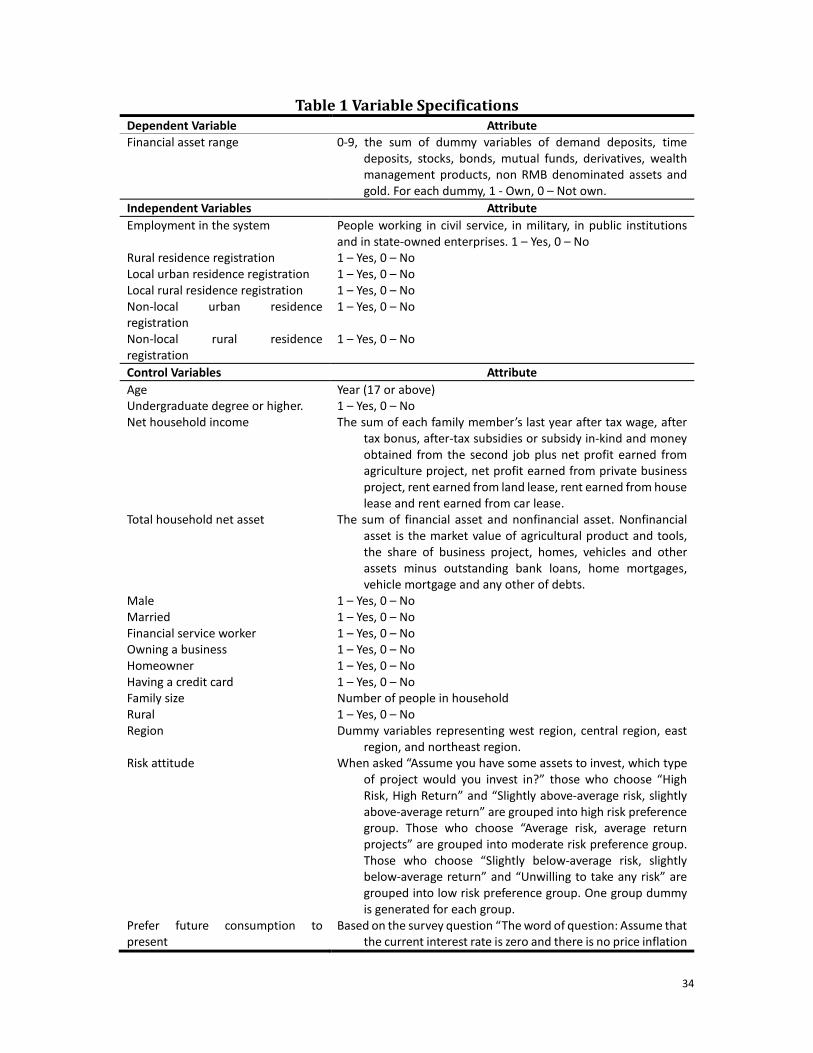
In this study, the dependent variable is the financial asset range representing financial

capability. In the 2011 CHFS survey, detailed data of financial assets of household is

available, including demand deposits, time deposits, stocks, bonds, mutual funds,

derivatives, wealth management products, non RMB denominated assets, and gold. We

created 9 dummy variables for these financial asset types. A dummy variable for each type

of financial asset was set to 1 if a household held that kind of asset and 0 otherwise. The

financial asset range is the sum of the 9 dummy variables, with possible scores from 0 to

9. For example, if a household only holds bonds, stocks, and gold, then its financial asset

range is 3.

The focused independent variables are employment type and household residence

registration status. If the interviewee works in civil service, the military, a public institution

or a state-owned enterprise, a dummy variable labeled ”employee in the system” was set

to 1, otherwise 0. Two sets of dummy variables of household residence registration status

were used, one set included urban registration and rural registration, and the other set

included local urban registration, local rural registration, non-local urban registration, and

non-local rural registration. We used the information of the household head to measure

the employment type and the household residence registration status.

Following the literature, control variables were age, net household income, net

15

household asset, family size, and several dummy variables including gender, marital status,

finance service worker status, owning a business, owning a home, possession of a credit

card, risk attitude when they were asked about investment risk preference, a set of regions,

and the preference for future vs. consumption. An endogeneity problem may occur

considering people living in the rural area might have less exposure to the financial

institution branches, which might lead to fewer financial assets. To address this issue, we

added a dummy variable indicating whether a household lives in the rural area. The

endogeneity problem may also derive from the omitted variable which is the unobserved

ability of individuals that may affect both government employment and financial

capability. We address this issue by including a dummy variable indicating whether an

individual has an undergraduate or higher degree, as a proxy of the unobserved ability of

individuals. In China, the college and graduate school entrance exams are very competitive.

We believe people who passed these entrance exams had better ability than others. See

Table 1 for more details of variable specifications.

[Insert Table 1 here]

3.3. Data Analysis

Bivariate analysis and multiple OLS regressions were used for preliminary analyses to

examine the relationship between financial capability and a set of independent variables.

Since the type of the dependent variable is count data, the model cannot be consistently

estimated with linear regression methods due to the preponderance of zeros (in this study,

37% of the observations is zero in dependent variable), and the nature of the discrete

choice dependent variable (Greene, 2012). Following the tradition in dealing with count

16

data, we used Poisson regression for more accurate analyses. The deviance goodness-of-

fit tests and Pearson goodness-of-fit tests did not reject the assumption which should be

satisfied for Poisson regression, meaning there was no over-dispersion (variance and

mean are not equal) in the dependent variable (StataCorp, 2013).

The distribution of financial asset range follows Poisson distribution:

P(FAR = k) = (𝜆𝜆k/k!)𝑒𝑒−𝜆𝜆 (1) where FAR is the financial asset range, representing financial capability and λ = E(FAR).

Denoting households by 𝑖𝑖, we estimate the following Poisson regression model:

log [𝜆𝜆(Y𝑖𝑖)] = X𝑖𝑖Β+ Z𝑖𝑖Γ + µ𝑖𝑖 (2) where Yi is the financial asset range, Xi is a vector of focused independent variables

including employment type and household registration status, Zi is a vector of control

variables and µi is the error term.

Seven models were used in the analyses. Model I, II, and III used bivariate and multiple

OLS regressions for key variable analyses, Model IV and VI used multiple OLS regressions

by adding control variables, and Model V and VII used Poisson regressions. Model

specifications are as follows:

Model I: Yi = β1x1i + µ1i (3)

Model II: Yi = β2x2i + µ2i (4)

Model III: Yi = β3x3i + β4x4i + β5x5i + µ3i (5)

Model IV: Yi = X1iΒ1 + ZiΓ1 + µ4i (6)

Model V: log [λ(Yi)] = X1iΒ2 + ZiΓ2 + µ5i (7)

Model VI: Yi = X2iΒ3 + ZiΓ3 + µ6i (8)

Model VII: log [λ(Yi)] = X2iΒ4 + ZiΓ4 + µ7i (9)

17

where Yi is the financial asset range; x1i is the indicator of employee in the system; x2i

is the indicator of rural household registration; x3i , x4i and x5i are the indicators of

local rural, non-local urban and non-local rural household residence registration

respectively; X1𝑖𝑖 is a vector of employee in the system and rural household registration;

X2𝑖𝑖 is a vector of employee in the system, local rural, non-local urban and non-local rural

household residence registration; Z𝑖𝑖 is a vector of control variables and µki (𝑘𝑘 =

1,2,3,4,5,6,7) is the error term.

4 Results

4.1. Descriptive Statistics

Table 2 presents descriptive statistics of financial asset holdings in the sample. As can be

seen, only 63% of households had at least one financial asset, 57% of households had

demand deposits and 18% of households had time deposits. Stock market participation

was merely 9% while 4% of household bought mutual funds. Compared to the U.S.

where 35% of general population had stocks, bonds, mutual funds or other securities

(FINRAIEF, 2012), the financial market participation in China was low.

[Insert Table 2 here]

Table 3 presents descriptive statistics of the financial asset range. 37% of households

had no financial assets at all. Most people (42%) had only one type of financial asset. Only

one household had seven types of financial assets and no household had more than seven

types.

[Insert Table 3 here]

As shown in Table 4, 11% of respondents were employees in the government-

18

managed working system, among which many worked in public service institution and

state-owned enterprises. A little over half of the households were registered in rural area

and less than 5% of households had non-local residence registration in either rural or

urban area.

[Insert Table 4 here]

Table 5 reports descriptive statistics of control variables. The average age of the

household heads was 50. As for education, 92% of household heads did not have an

undergraduate degree meaning that the average education level of Chinese people was

still low. Approximately 74% of household heads in Chinese families were male. Data

showed that 90% of families owned their home. Only 14% of household heads used credit

cards. 61% of the household heads interviewed were in the low risk preference group.

[Insert Table 5 here]

4.2. Results of Regression Analysis

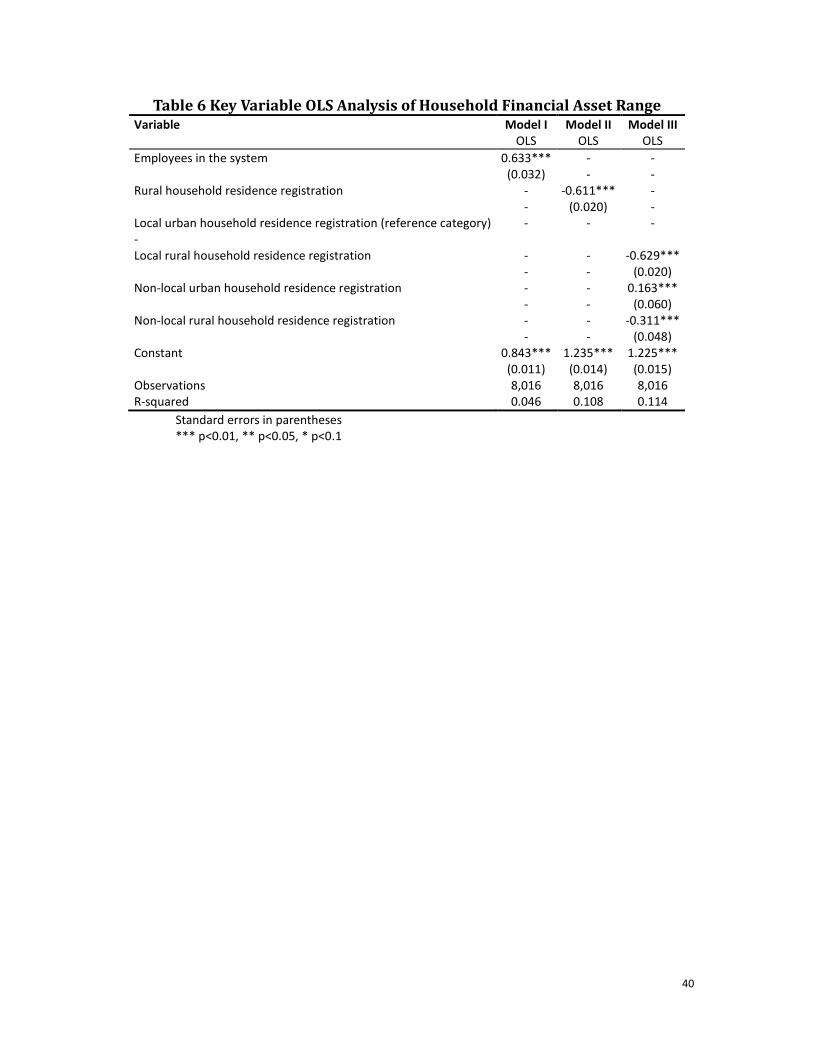
In Table 6, we found in bivariate analysis (Model I), the coefficient of employment in the

system variable was significantly positive. In Model II, people with rural registration had a

significantly smaller financial asset range. In Model III, people with non-local registration

had a significantly larger financial asset range compared to people with local registration

in both urban and rural group. In both local and non-local groups, people with rural

registration had significantly smaller financial asset ranges, which confirmed the result of

Model II.

[Insert Table 6 here]

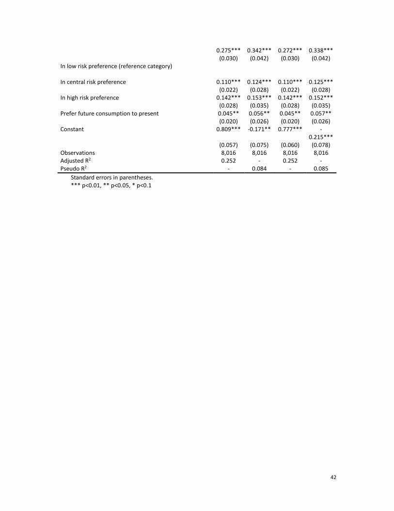
Table 7 presents results of multiple regressions by adding control variables. The

19

results were as expected. In all four models, the effect of employment in the system on

the household financial asset range was significantly positive. Results of two sets of OLS

regressions were similar. The findings suggested that people employed in the

government-managed system had better financial capability than those employed in

collective and private owned enterprises, supporting H1.

[Insert Table 7 here]

Results of both Models IV and V showed that the rural household residence

registration was negatively associated with the household financial asset range,

suggesting people with rural household residence registration had lower financial

capability compared to their urban counterparts and supporting H2.

Results regarding H3 are interesting. After adding control variables in Models VI and

VII, the coefficients of non-local urban household residence registration became negative

and not significant, while in Model III it was significantly positive without control variable.

We speculate the result of Model III may be resulted from the higher education level of

people with non-local urban registration compared to those with local urban registration.

With this data set, we translated the education into years of schooling according to China’s

education system, and found that on average, people with local urban registration had 9.6

years of school while people with non-local urban registration had 13.2 years of school.

After controlling for education, the advantage of people with non-local urban registration

in terms of financial capability became insignificant. In either case, H3 was not supported.

In model VII, both coefficients of local and non-local rural registrations were

significantly negative and the coefficient of non-local rural registration was smaller than

20

local rural registration, suggesting people with non-local rural registration had better

financial capability and supporting H4. To provide a more direct test, we conducted an

additional analysis similar to model VII with one change, using the local rural people as

the reference group, and found that the coefficient of non-local rural group was

significantly positive (The table is not presented here but available upon requests).

Some control variables provided signs consistent with our expectations. Age, having

undergraduate or higher degree, net household asset, marriage, being a financial service

worker, owning a home, having a credit card, being in higher preference of risk group and

preferring future consumption than present all had positive effects on the financial asset

range. However in our study, gender was not significant. Since net household income was

significantly positively correlated with household asset, when household asset entered

into the regression with household income, household income lost its significance.

Owning a business was positively associated with the dependent variable in all four

models but not significant in OLS regressions. Geographically, people in the east region

had larger average financial asset ranges, followed by people in the central region and

west region. It was consistent with our understanding that the east of China is the most

economically developed area, as the average annual income per capita of urban

households in the east is about 50% higher than that in the central and west (Xu and Kong,

2015). What is shocking is that people in the northeast region had the lowest average

financial asset range, even lower than people in the central and west. It reflected the

common belief that the northeast region, the former industrial power house, was a

rustbelt today and needs to be revitalized.

21

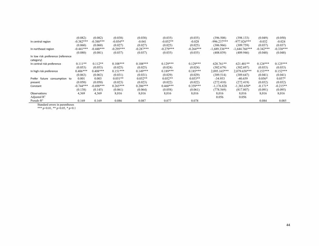
4.3. Robustness Checks

To ensure the robustness of our results to alternative measures and methods, we

performed several additional tests, the results of which can be found in the Table 8. First,

we used the ratio of financially risky asset to total financial asset as a second alternative

dependent variable and conducted the Tobit regression, given that the financially risky

asset ratio lied within the range between 0 and 1. Financially risky assets were measured

by total market value of financial asset excluding demand deposit, time deposit, state

bond and local government bond. By using financially risky asset, we placed more

emphasis on the risky assets since investment in risky assets requires more

comprehensive financial knowledge. In the construction of the second alternative

dependent variable, we added a dummy variable indicating whether a household had a

non-primary housing to the financial asset range, since the non-primary housing is usually

considered as an investment and the purchase of property requires some degree of

financial capability. We generated a third alternative dependent variable by adding a

dummy variable indicating whether a household had its own business. Thus, we

accounted for the roles of owning a home and a business in the computation of financial

capabilities. The main results of Model VIII to Model XIII were qualitatively consistent with

those in Table 7.

In addition, we constructed the weighted financial asset to account for the roles of

different riskiness of each financial asset and its share in the portfolio. The accurate

calculation was difficult because the data of exact risks of the nine financial asset

instruments were not available. Thus we used the variance of the monthly return rate of

22

each financial asset in 2011 as proxies for the risk of each financial asset. The annual

interest rates of demand deposit and one-year time deposit published by the People's

Bank of China were used to generate the monthly interest rate for demand deposit and

time deposit. We used the monthly average of the CSI 300 Index, a capitalization-weighted

stock market index designed to replicate the performance of 300 stocks traded in the

Shanghai and Shenzhen Stock Exchanges, to represent the market performance of the

stocks in general; the monthly average of the Shanghai Stock Exchange treasure index

settlement price to represent the market performance of the bonds in general; the

monthly average of Shanghai Stock Exchange funds index settlement price to represent

the market performance of the mutual funds in general; the Shanghai Stock Exchange

financial futures monthly settlement price to represent the market performance of the

derivatives in general; the monthly average of the price of the US dollar in RMB published

by the People's Bank of China to represent the market performance of the non RMB

denominated assets in general; the monthly average gold price in RMB published by the

World Gold Council to represent the market performance of the gold. With the monthly

market performance of these six financial assets, we generated the monthly return rate

by the following equation:

MRR𝑖𝑖,𝑡𝑡 = (MP𝑖𝑖,𝑡𝑡 − MP𝑖𝑖,𝑡𝑡−1)/MP𝑖𝑖,𝑡𝑡−1; (10)

where MRR𝑖𝑖,𝑡𝑡 is the monthly return rate of asset 𝑖𝑖 in month 𝑡𝑡 and MP𝑖𝑖,𝑡𝑡 is the

market performance of asset 𝑖𝑖 in month 𝑡𝑡. The monthly return rate is comparable to the

monthly interest rates of demand deposit and time deposit. We then computed the

variance of the monthly return rate of each financial asset and generated weights for each

23

financial asset using the following equation:

ω𝑖𝑖 = σi

2/∑σi

2; (11)

where ω𝑖𝑖 is the weight for the financial asset 𝑖𝑖 and σi

2 is the variance of the monthly

return rate of financial asset 𝑖𝑖. Therefore the weighted financial asset was constructed by:

𝑊𝑊𝑊𝑊𝑊𝑊 = ∑ω𝑖𝑖 MV𝑖𝑖 (12)

where 𝑊𝑊𝑊𝑊𝑊𝑊 is the weighted financial asset and MV𝑖𝑖 is the market value of the financial

asset 𝑖𝑖. Since we could not find any data for the wealth management product, following

our understanding that the riskiness of a wealth management product lies between time

deposit and bonds, we used the average variance of time deposit and bonds to proxy the

variance of wealth management product and generate its weight accordingly. We

removed total household net asset because the weighted financial asset measured the

financial asset of the household, which was a substantial part of total household net asset.

The patterns of Model XIV and Model XV were the similar to the results of baseline

regressions.

Second, we conducted the negative binomial regression, given the nature of the

financial asset range measure. Negative binomial model and Poisson model are normally

adopted for the analyses of discrete choice dependent variables. Negative binomial model

relaxes the Poisson assumption that the mean equals the variance (Greene, 2012). Though

the deviance goodness-of-fit tests and Pearson goodness-of-fit tests showed that there

was no over-dispersion and Poisson regression was appropriate, we used negative

binomial regression as robustness checks for Poisson regression results. The results of

24

Model XVI and Model XVII in Table 8 were largely consistent with our Poisson analyses in

Table 7. The results of robustness checks are presented in the Table 8.

5 Conclusions

In this paper we examine the factors associated with Chinese consumer financial

capability measured by the household financial asset range from the perspective of

background risks with emphases on two independent variables with unique Chinese

features, employment type and household residential registration status. We have

achieved our research objectives that are to explore if there are differences in financial

capability between people working in two different types of working systems and

between people with different household residency registrations. We find employees in

the government-managed working system and people having urban residence registration

have better financial capability. Among people with rural residence registrations, non-

local people have better financial capability. Consumer with young age, having low income,

without undergraduate or higher degree, not using a credit card, working in non-financial

service occupations and living in the northeast region tend to have a lower level of

financial capability.

The limitation of this study is that we do not investigate mechanisms between the

two focused independent variables and financial capability because it can be complicated

and beyond the scope of this paper. In addition, some control variables such as owning a

business and gender show results different from previous research using data of

developed countries. These issues could be addressed in future research.

The results of this study are informative for helping consumer financial educators to

25

identify vulnerable consumers in the financial market. Understanding the employment

type and residence registration differences in financial capability helps financial educators

provide pertinent education to Chinese consumers with diverse needs. Consumer

educators should be aware of differences in financial literacy, behavior, and capability

among consumers with diverse backgrounds. To increase effectiveness in financial

education, financial educators should provide tailored education for vulnerable

consumers with low income and low education, not using a credit card, working in non-

financial service occupations and private sectors, and living in the rural areas and less

developed regions in China. If possible, basic financial education should be provided in

junior high or high school as most people do not go to college.

26

Acknowledgement

The China Scholarship Council provided the support for Mr. Xu Cui, a doctoral student

from School of Busniess, Renmin University of China, for his research as a visiting scholar

at the University of Rhode Island with a scholarship (grant number [2016]3100). We thank

Deborah Kopech for her assistance in copy editing.

27

References

Abreu, M. and V. Mendes (2010). Financial Literacy and Portfolio Diversification.

Quantitative Finance, 10(5), 515-528.

Afridi, F., Li, S. X., and Y. Ren (2015). Social Identity and Inequality: The Impact of China's

Hukou System. Journal of Public Economics, 123, 17-29.

Atkinson, A., McKay, S., Collard, S. and E. Kempson (2006). Levels of Financial Capability in

the UK: Results of a Baseline Survey. Financial Services Authority, London.

Bai, C. E., Lu, J. and Z. Tao (2009). How Does Privatization Work in China? Journal of

Comparative Economics, 37(3), 453-470.

Brødsgaard, K. E. (2002). Institutional Reform and the Bianzhi System in China. The China

Quarterly, 170, 361-386.

Cai, Y. and Y. Cheng (2014). Pension Reform in China: Challenges and Opportunities.

Journal of Economic Surveys, 28(4), 636-651.

Cardak, B. A. and R. Wilkins (2009). The Determinants of Household Risky Asset Holdings:

Australian Evidence on Background Risk and Other Factors. Journal of Banking and

Finance, 33(5), 850-860.

Chan, K. W. (2010). The Household Registration System and Migrant Labor in China: Notes

on a Debate. Population and Development Review, 36(2), 357-364.

Chan, K. W. and Buckingham, W. (2008). Is China Abolishing the Hukou System?. The China

Quarterly, 195, 582-606.

Chinanews. 2016 Oct 24. The 2017 Annual National Examination Application Ended with

the Admission Rate of the Hottest Post Being "One in Ten Thousand". Retrieved

28

from http://www.chinanews.com/gn/2016/10-24/8042039.shtml

Cheng, T., and M, Selden. (1994). The Origins and Social Consequences of China's Hukou

System. The China Quarterly, 139, 644-668.

Cui, F., Ge, Y. and F. Jing (2013). The Effects of the Labor Contract Law on the Chinese Labor

Market. Journal of Empirical Legal Studies, 10(3), 462-483.

Cui, Y., Nahm, D., and M. Tani (2015). Employment Choice and Ownership Structure in

Transitional China. The Singapore Economic Review, Vol. 60, No. 4 ,1550088. DOI:

10.1142/S0217590815500885

Deidda, M. (2014). Does Portfolio Diversification Mitigate Financial Risk? Evidence from

Italian Survey Data. Rivista Italiana Degli Economisti, 19(3), 393-420.

Du, J. (2009). Economic Reforms and Health Insurance in China. Social Science & Medicine,

69(3), 387-395.

Fang, Z., and Sakellariou, C. (2016). Social Insurance, Income and Subjective Well-Being of

Rural Migrants in China—An Application of Unconditional Quantile Regression.

Journal of Happiness Studies, 17(4), 1635-1657.

FINRAIEF. (2013) Financial capability in the United States: Report of findings from the 2012

National Financial Capability Study. FINRA Investor Education Foundation,

Washington, DC.

Fu, J. (2014). To Start a Business or to Pursue for a “Bianzhi”? Empirical Analysis of Income

Differences Between Self-employers and Officials. Shanghai Economic Review. (6),

93-102.

Gan, L. Yin, Z. H. Jia, N. Xu, S.and S. Ma (2013). Data You Need to Know about China.

29

Springer.

Gao, Q., Ying, Q. and D. Luo (2015). Hidden Income and Occupational Background:

Evidence from Guangzhou. Journal of Contemporary China, 24(94), 721-741.

Georgarakos, D. and R. Inderst (2011). Financial Advice and Stock Market Participation.

European Central Bank, Working Paper Series: 1296.

Greene, William H. (2012). Econometric Analysis (Seventh Edition). New Jersey: Prentice-

Hall.

Guiso, L. and T. Jappelli (2008) Financial Literacy and Portfolio Diversification. CSEF

Working Papers 212, Centre for Studies in Economics and Finance, Naples (Italy).

Haliassos, M. and C.C. Bertaut (1995). Why Do so Few Hold Stocks? Economic Journal, 105,

1110–1129.

Han, L., Chen, H. S. and C. G. Liu (2016) Is There Intergeneration Transmission of the “Iron

Rice Bowl”? Empirical Analysis of Chinese Bianzhi Job Post. Economic Perspectives,

(8), 61-70.

He, L. X., Wu, H. J. and Z. G. Zhang (2015). Analysis on the Income Difference between

Non-local Migrant Workers and Local Migrant Workers -- Based on the Perspective of

Household Registration. Journal of Agrotechnical Economics, (6), 15-26.

Heaton, J. and D. Lucas (2000). Portfolio Choice and Asset Prices: The Importance of

Entrepreneurial Risk. Journal of Finance, 55(3), 1163-1198.

Hochguertel, S. (2003). Precautionary Motives and Portfolio Decisions. Journal of Applied

Econometrics, 18, 61–77.

Jappelli, T. and M. Padula (2015). Investment in Financial Literacy, Social Security and

30

Portfolio Choice. Journal of Pension Economics and Finance, 14(4), 369-411.

Li, P. and F. Tian (2011). New generation of farmer workers in China: Social attitude and

behavior choice. Society, 31(3), 1–21.

Lin, J. T., Bumcrot, C., Ulicny, T., Lusardi, A., Mottola, G., Kieffer, C. and G. Walsh (2016).

Financial Capability in the United States: Report of Findings from the 2015 National

Financial Capability Study. FINRA Investor Education Foundation, Washington, DC.

Retrieved from http://gflec.org/wp-

content/uploads/2016/07/NFCS_2015_Report_Natl_Findings.pdf

Lusardi, A., and O. S. Mitchell (2011). Financial Literacy and Retirement Planning in the

United States. Journal of Pension Economics and Finance, 10(4), 509-525.

Lusardi, A., and O. S. Mitchell (2014). The Economic Importance of Financial Literacy:

Theory and Evidence. Journal of Economic Literature, 52(1), 5-44.

Markowitz, H. (1952). Portfolio Selection. The Journal of Finance, 7(1), 77-91.

National Bureau of Statistics of China. (2016). China Statistical Yearbook-2016. Retrieved

from http://www.stats.gov.cn/tjsj/ndsj/2016/indexeh.htm

National People's Congress of the People's Republic of China. (1958). The ordinance of

household registration of the People's Republic of China (Zhong Hua Ren Min Gong

He Guo Hu Kou Deng Ji Tiao Li). Promulgated at the nighty-first Session of the

Standing Committee of the National People's Congress on January 9th, 1958.

Retrieved from http://www.npc.gov.cn/wxzl/gongbao/2000-

12/10/content_5004332.htm.

OECD. (2016). Financial Education in Europe: Trends and Recent Developments. OECD

31

Publishing, Paris.

Robb, C. A., and A. S. Woodyard (2011). Financial Knowledge and Best Practice Behavior.

Journal of Financial Counseling and Planning, 22(1), 60-70, 86-87.

Rosen, H.S. and S. Wu (2004). Portfolio Choice and Health Status. Journal of Financial

Economics, 72, 457–484.

Shi, S. J. and K. H. Mok (2012). Pension Privatisation in Greater China: Institutional Patterns

and Policy Outcomes. International Journal of Social Welfare, 21(s1), S30-S45.

Sonoda, T. (2014). Why Do Household Heads In Rural China Not Work More In The Market?

The Singapore Economic Review, 59(01), 1450008. DOI:

10.1142/S0217590814500088

StataCorp. (2013). Stata 13 Base Reference Manual. College Station, TX: Stata Press. 1640.

Taylor, M. (2011). Measuring Financial Capability and Its Determinants Using Survey Data.

Social Indicators Research, 102, 297–314.

The Peoples’ Bank of China. (2013, August 27). The Peoples’ Bank of China Promotes

Financial Literacy Month Program. Retrieved from http://www.gov.cn/gzdt/2013-

08/27/content_2474944.htm

Tsigos, S., & Daly, K. (2016). “Fair go” for all? Wealth and Risk Aversion of Australian

Households. Australian Economic Papers, 55(3), 274-300.

Van Rooij, M., Lusardi, A., and R. Alessie (2011). Financial Literacy and Stock Market

Participation. Journal of Financial Economics, 101(2), 449-472.

Wang, Y. J., Liu, Y. L., Li, Z. B., Xing, C. B., Cui, X. Y. and C. Jiang (2016). Household

Registration and College Students' Employment: An Empirical Research Based on

32

Sampling Survey Data of Employment Situation of College Graduates. Studies in

Labor Economics, (2), 72-94.

Wong, K., Fu, D., Li, C. Y., and H. X. Song (2007). Rural Migrant Workers in Urban China:

Living a Marginalised Life. International Journal of Social Welfare, 16(1), 32-40.

Wu, W. (2006). Migrant Intra-urban Residential Mobility in Urban China. Housing Studies,

21(5), 745-765.

Xiao, J. J., Chen, C. and F. Chen (2014). Consumer Financial Capability and Financial

Satisfaction. Social Indicators Research, 118(1), 415-432.

Xiao, J. J., Chen, C. and L. Sun (2015). Age differences in consumer financial capability.

International Journal of Consumer Studies, 39, 387–395.

Xie, G. H. (2012). Human Capital Return and Social Integration of Migrant Population in

China. Social Sciences in China, 04, 103-124.

Xu, J. and D. Kong (2015). Understanding the Household Consumption Behavior in Urban

China. The Singapore Economic Review, 60(05), 1550062. DOI:

10.1142/S0217590815500629

Yin, Z. C., Song, Q. Y. and Y. Wu (2014). Financial Literacy, Trading Experience and

Household Portfolio Choice. Economic Research, 04, 62-75.

Zhang, M. and R. Rasiah, (2014). Institutional Change and State Owned Enterprises in

China's Urban Housing Market. Habitat International, 41, 58-68.

Zhang, Y., Filipski, M. J., and K. Z. Chen (2016). Health Insurance and Medical

Impoverishment in Rural China: Evidence from Guizhou Province. The Singapore

Economic Review, Vol. 62, No. 1, 1650017. DOI: 10.1142/S021759081650017X

33

Zhang, Z., and D. J. Treiman (2013). Social Origins, Hukou Conversion, and the Wellbeing

of Urban Residents in Contemporary China. Social Science Research, 42(1), 71-89.

Zhu, L. (2003). The hukou system of the People's Republic of China: a critical appraisal

under International Standards of Internal Movement and Residence. Chinese Journal

of International Law, 2(2), 519-566.

34

Table 1 Variable Specifications Dependent Variable Attribute Financial asset range 0-9, the sum of dummy variables of demand deposits, time

deposits, stocks, bonds, mutual funds, derivatives, wealth management products, non RMB denominated assets and gold. For each dummy, 1 - Own, 0 – Not own.

Independent Variables Attribute Employment in the system People working in civil service, in military, in public institutions

and in state-owned enterprises. 1 – Yes, 0 – No Rural residence registration 1 – Yes, 0 – No Local urban residence registration 1 – Yes, 0 – No Local rural residence registration 1 – Yes, 0 – No Non-local urban residence registration

1 – Yes, 0 – No

Non-local rural residence registration

1 – Yes, 0 – No

Control Variables Attribute Age Year (17 or above) Undergraduate degree or higher. 1 – Yes, 0 – No Net household income The sum of each family member’s last year after tax wage, after

tax bonus, after-tax subsidies or subsidy in-kind and money obtained from the second job plus net profit earned from agriculture project, net profit earned from private business project, rent earned from land lease, rent earned from house lease and rent earned from car lease.

Total household net asset The sum of financial asset and nonfinancial asset. Nonfinancial asset is the market value of agricultural product and tools, the share of business project, homes, vehicles and other assets minus outstanding bank loans, home mortgages, vehicle mortgage and any other of debts.

Male 1 – Yes, 0 – No Married 1 – Yes, 0 – No Financial service worker 1 – Yes, 0 – No Owning a business 1 – Yes, 0 – No Homeowner 1 – Yes, 0 – No Having a credit card 1 – Yes, 0 – No Family size Number of people in household Rural 1 – Yes, 0 – No Region Dummy variables representing west region, central region, east

region, and northeast region. Risk attitude When asked “Assume you have some assets to invest, which type

of project would you invest in?” those who choose “High Risk, High Return” and “Slightly above-average risk, slightly above-average return” are grouped into high risk preference group. Those who choose “Average risk, average return projects” are grouped into moderate risk preference group. Those who choose “Slightly below-average risk, slightly below-average return” and “Unwilling to take any risk” are grouped into low risk preference group. One group dummy is generated for each group.

Prefer future consumption to present

Based on the survey question “The word of question: Assume that the current interest rate is zero and there is no price inflation

35

to be factored in, which of the following payments would you prefer, 1000 RMB on tomorrow or 1100 RMB in one year?” 1- Get 1100 a year from now, 0 - Get 1000 RMB tomorrow

36

Table 2 Details of Financial Asset Holdings (N=8,016) Types of Financial Asset Frequency Percent Std. Dev.

Demand deposits 4546 56.71% 0.50 Time deposits 1443 18.00% 0.38 Stocks 722 9.01% 0.29 Bonds 63 0.79% 0.09 Mutual funds 346 4.32% 0.20 Derivatives 4 0.05% 0.02 Wealth management products 67 0.84% 0.09 Non RMB denominated assets 88 1.10% 0.10 Gold 52 0.65% 0.08 Holding any of above 5039 62.86% -

37

Table 3 Details of Financial Asset Range Count Variable Financial asset range

Value 0 1 2 3 4 5 6 7 Total

Frequency 2,977 3,360 1,236 324 82 24 12 1 8016 Percent 37.14% 41.92% 15.42% 4.04% 1.02% 0.30% 0.15% 0.01% 100.00%

38

Table 4 Descriptive Statistics of Employment Type and Household Registration Status Frequency Percentage Employees in the system 900 11.23% Fiscally dependent employees 555 6.92% In government 141 1.76% In public service institution 409 5.10% In military 5 0.06% In state-owned enterprises 392 4.89% Employees not in the system 7116 88.77% Urban household residence registration 3810 47.53% Local urban registration 3581 44.67% Non-local urban registration 229 2.86% Rural household residence registration 4206 52.47% Local rural registration 3844 47.95% Non-local rural registration 362 4.52%

39

Table 5 Descriptive Statistics (N=8016) Mean Std. Dev.

Age 49.84 13.99 Net household income (yuan) 26121.21 142319.00 Total household net asset (yuan) 466122.70 959908.90 Family size 3.48 1.54

Frequency Percentage

Undergraduate degree or higher 649 8.10% Male 5875 73.29% Married 7001 87.34% Financial service worker 224 2.79% Owning a business 1020 12.72% Homeowner 7291 90.96% Having a credit card 1132 14.12% Rural 3072 38.32% In west region 1184 14.77% In central region 2412 30.09% In east region 3418 42.64% In northeast region 1002 12.50% In low risk preference group 4869 60.74% In moderate risk preference group 2069 25.81% In high risk preference group 1078 13.45% Prefer future consumption to present 2352 29.34%

40

Table 6 Key Variable OLS Analysis of Household Financial Asset Range Variable Model I Model II Model III OLS OLS OLS Employees in the system 0.633*** - - (0.032) - - Rural household residence registration - -0.611*** - - (0.020) - Local urban household residence registration (reference category) - - - - Local rural household residence registration - - -0.629*** - - (0.020) Non-local urban household residence registration - - 0.163*** - - (0.060) Non-local rural household residence registration - - -0.311*** - - (0.048) Constant 0.843*** 1.235*** 1.225*** (0.011) (0.014) (0.015) Observations 8,016 8,016 8,016 R-squared 0.046 0.108 0.114

Standard errors in parentheses *** p<0.01, ** p<0.05, * p<0.1

41

Table 7 Results of Regressions on Household Financial Asset Range Variable Model IV Model V Model VI Model

VII OLS Poisson OLS Poisson Employees in the system 0.160*** 0.129*** 0.160*** 0.129***

(0.032) (0.035) (0.033) (0.035) Rural household residence registration -

0.302*** -

0.367***

(0.024) (0.032) Local urban household residence registration (reference category)

Local rural household residence registration -0.321***

-0.403***

(0.026) (0.035) Non-local urban household residence registration -0.007 -0.008

(0.056) (0.060) Non-local rural household residence registration -

0.205*** -

0.218*** (0.047) (0.061)

Age 0.000 0.000 0.001 0.001 (0.001) (0.001) (0.001) (0.001)

Undergraduate degree or higher 0.226*** 0.126*** 0.231*** 0.132*** (0.038) (0.039) (0.038) (0.039)

Net household income 0.000 0.000 0.000 0.000 (0.000) (0.000) (0.000) (0.000)

Total household net asset 0.000*** 0.000*** 0.000*** 0.000*** (0.000) (0.000) (0.000) (0.000)

Male 0.031 0.036 0.032 0.038 (0.021) (0.027) (0.021) (0.027)

Married 0.123*** 0.135*** 0.124*** 0.136*** (0.029) (0.039) (0.029) (0.039)

Family size -0.016** -0.019** -0.015** -0.017* (0.007) (0.009) (0.007) (0.009)

Financial service worker 0.254*** 0.160*** 0.255*** 0.161*** (0.056) (0.055) (0.056) (0.055)

Owning a business -0.019 0.012 -0.020 0.009 (0.028) (0.036) (0.028) (0.036)

Homeowner 0.055* 0.086** 0.063* 0.097** (0.033) (0.043) (0.033) (0.044)

Credit card 0.380*** 0.299*** 0.381*** 0.300*** (0.030) (0.033) (0.030) (0.033)

Rural -0.178***

-0.281***

-0.166***

-0.260***

(0.024) (0.034) (0.025) (0.035) In east region (reference category)

In west region -

0.077*** -

0.128*** -0.072** -

0.120*** (0.029) (0.042) (0.029) (0.042)

In central region -0.007 -0.032 -0.000 -0.024 (0.023) (0.030) (0.023) (0.030)

In northeast region - - - -

42

0.275*** 0.342*** 0.272*** 0.338*** (0.030) (0.042) (0.030) (0.042)

In low risk preference (reference category)

In central risk preference 0.110*** 0.124*** 0.110*** 0.125*** (0.022) (0.028) (0.022) (0.028)

In high risk preference 0.142*** 0.153*** 0.142*** 0.152*** (0.028) (0.035) (0.028) (0.035)

Prefer future consumption to present 0.045** 0.056** 0.045** 0.057** (0.020) (0.026) (0.020) (0.026)

Constant 0.809*** -0.171** 0.777*** -0.215***

(0.057) (0.075) (0.060) (0.078) Observations 8,016 8,016 8,016 8,016 Adjusted R2 0.252 - 0.252 - Pseudo R2 - 0.084 - 0.085

Standard errors in parentheses. *** p<0.01, ** p<0.05, * p<0.1

43

Table 8 Robustness Checks Model VIII Model IX Model X Model XI Model XII Model XIII Model XIV Model XV Model XVI Model XVII Dependent Variable Risky Asset

Ratio Risky Asset

Ratio Financial Asset Range plus Non Primary Home

Financial Asset Range plus Non Primary Home

Financial Asset Range plus Non Primary

Home and Business

Financial Asset Range plus Non Primary

Home and Business

Weighted Financial Asset

Weighted Financial Asset

Financial Asset Range

Financial Asset Range

Model

Independent Variables

Tobit Tobit Poisson Poisson Poisson Poisson OLS OLS Negative Binomial

Negative Binomial

Employees in the system 0.219*** 0.209*** 0.126*** 0.130*** 0.064** 0.067** 839.706* 905.404** 0.129*** 0.129*** (0.060) (0.060) (0.032) (0.032) (0.031) (0.031) (443.939) (445.845) (0.042) (0.042)

Rural household residence registration

-0.535*** -0.315*** -0.377*** -1,218.814*** -0.367*** (0.064) (0.029) (0.024) (330.965) (0.039)

Local urban household residence registration (reference category)

Local rural household residence registration

-0.547*** -0.356*** -0.424*** -1,109.604*** -0.403*** (0.070) (0.031) (0.025) (350.635) (0.042)

Non-local urban household residence registration

-0.131 0.037 0.035 1,263.510 -0.008 (0.098) (0.052) (0.050) (773.996) (0.073)

Non-local rural household residence registration

-0.560*** -0.137*** -0.086* -1,271.443** -0.218*** (0.113) (0.052) (0.047) (647.666) (0.081)

Age -0.003* -0.004** -0.001 -0.000 -0.005*** -0.003*** 30.444*** 31.904*** 0.000 0.001 (0.002) (0.002) (0.001) (0.001) (0.001) (0.001) (9.944) (10.184) (0.001) (0.001)

Undergraduate degree or higher -0.117* -0.112* 0.103*** 0.108*** 0.029 0.043 2,489.525*** 2,420.089*** 0.126*** 0.132*** (0.066) (0.066) (0.035) (0.035) (0.034) (0.034) (521.063) (522.874) (0.045) (0.045)

Net household income 0.000 0.000 0.000 0.000 0.000** 0.000** 0.007*** 0.007*** 0.000 0.000 (0.000) (0.000) (0.000) (0.000) (0.000) (0.000) (0.001) (0.001) (0.000) (0.000)

Total household net asset 0.000*** 0.000*** 0.000*** 0.000*** 0.000*** 0.000*** 0.000*** 0.000*** (0.000) (0.000) (0.000) (0.000) (0.000) (0.000) (0.000) (0.000)

Male -0.072 -0.070 0.020 0.022 0.012 0.018 -701.841** -723.746** 0.036 0.038 (0.049) (0.049) (0.024) (0.024) (0.023) (0.023) (292.620) (292.913) (0.032) (0.032)

Married 0.080 0.074 0.033 0.037 0.045 0.051 549.229 589.044 0.135*** 0.136*** (0.071) (0.071) (0.033) (0.033) (0.032) (0.032) (397.808) (398.653) (0.047) (0.047)

Family size -0.023 -0.024 -0.013 -0.009 -0.001 0.005 -36.063 -32.760 -0.019* -0.017 (0.019) (0.019) (0.008) (0.008) (0.008) (0.008) (89.098) (89.489) (0.011) (0.011)

Financial service worker 0.137 0.139 0.141*** 0.143*** 0.093* 0.095** 513.980 510.256 0.160** 0.161** (0.094) (0.094) (0.050) (0.050) (0.048) (0.048) (768.098) (768.080) (0.067) (0.067)

Owning a business 0.032 0.035 0.078** 0.073** 47.877 39.573 0.012 0.009 (0.067) (0.067) (0.032) (0.032) (383.318) (383.529) (0.045) (0.045)

Homeowner 0.164** 0.158* 1,013.886** 1,044.856** 0.086* 0.097* (0.081) (0.082) (444.236) (447.657) (0.051) (0.051)

Credit card 0.424*** 0.424*** 0.286*** 0.287*** 0.275*** 0.277*** 3,699.380*** 3,681.254*** 0.299*** 0.300*** (0.056) (0.056) (0.030) (0.030) (0.028) (0.028) (408.953) (409.078) (0.038) (0.038)

Rural -0.331*** -0.326*** -0.284*** -0.258*** 316.222 275.805 -0.281*** -0.260*** (0.072) (0.073) (0.031) (0.031) (329.707) (336.981) (0.041) (0.042)

In east region (reference category)

In west region -0.150* -0.153* -0.156*** -0.144*** -0.237*** -0.208*** -1,129.637*** -1,117.139*** -0.128*** -0.120**

44

(0.082) (0.082) (0.038) (0.038) (0.035) (0.035) (396.508) (398.133) (0.049) (0.050) In central region -0.382*** -0.388*** -0.054** -0.041 -0.052** -0.028 -996.237*** -977.826*** -0.032 -0.024

(0.060) (0.060) (0.027) (0.027) (0.025) (0.025) (306.966) (309.759) (0.037) (0.037) In northeast region -0.441*** -0.448*** -0.295*** -0.287*** -0.279*** -0.264*** -1,689.336*** -1,644.766*** -0.342*** -0.338***

(0.080) (0.081) (0.037) (0.037) (0.035) (0.035) (408.039) (409.946) (0.048) (0.048) In low risk preference (reference category)

In central risk preference 0.111** 0.112** 0.108*** 0.108*** 0.129*** 0.129*** 628.761** 621.401** 0.124*** 0.125*** (0.053) (0.053) (0.025) (0.025) (0.024) (0.024) (302.679) (302.697) (0.033) (0.033)

In high risk preference 0.406*** 0.408*** 0.151*** 0.149*** 0.189*** 0.185*** 2,095.165*** 2,079.658*** 0.153*** 0.152*** (0.063) (0.063) (0.031) (0.031) (0.029) (0.029) (389.514) (389.647) (0.041) (0.041)

Prefer future consumption to present

0.001 0.003 0.051** 0.052** 0.052** 0.053** -34.953 -40.659 0.056* 0.057* (0.050) (0.050) (0.023) (0.023) (0.022) (0.022) (272.410) (272.419) (0.032) (0.032)

Constant -0.744*** -0.698*** 0.265*** 0.206*** 0.460*** 0.359*** -1,176.828 -1,383.650* -0.171* -0.215** (0.138) (0.145) (0.061) (0.064) (0.058) (0.061) (778.569) (817.807) (0.091) (0.095)

Observations 4,369 4,369 8,016 8,016 8,016 8,016 8,016 8,016 8,016 8,016 Adjusted R2 0.056 0.056 Pseudo R2 0.169 0.169 0.086 0.087 0.077 0.078 0.084 0.085

Standard errors in parentheses *** p<0.01, ** p<0.05, * p<0.1