Page 1
End-of-Life Inventory Problem with Phase-out Returns
M. Pourakbar†, E. van der Laan‡, R. Dekker†∗
† Erasmus School of Economics, ‡ Rotterdam School of Management
Erasmus University Rotterdam
†Burgemeester Oudlaan 50, 3000DR Rotterdam, the Netherlands
[email protected] , [email protected] , [email protected]
* Phone: (+31)10-4081274, Fax: (+31)10-4089162
Econometric Institute Report EI 2011-12
Abstract
We consider the service parts end-of-life inventory problem of a capital goods manufac-
turer in the final phase of its life cycle. The final phase starts as soon as the production of parts
terminates and continues till the last service contract expires. Final order quantities are con-
sidered a popular tactic to sustain service fulfillment obligations and to mitigate the effect of
obsolescence. In addition to the final order quantity, other sources to obtain serviceable parts
are repairing returned defective items and retrieving parts from phase-out returns. Phase-out
returns happen when a customer replaces an old system platform with a next generation one
and returns the old product to the original equipment manufacturer (OEM). These returns can
well serve the demand for service parts of other customers still using the old generation of the
product. In this paper, we study the decision making complications stemming from phase-out
occurrence. We use a finite horizon Markov decision process to characterize the structure of
1
Page 2
the optimal inventory control policy. We show that the optimal policy consists of a time vary-
ing threshold level for item repair. Furthermore, we study the value of phase-out information
by extending the results to cases with an uncertain phase-out quantity or an uncertain sched-
ule. Numerical analysis sheds light on the advantages of the optimal policy compared to some
heuristic policies.
Keywords: End-of-life inventory management, spare parts, phase-out returns
1 Introduction
Due to the spurt of technology and innovation the service life cycle of both parts and products
have become shorter. Consequently, managing the inventories of service parts in order to fulfill
service obligations and avoid obsolescence risk has become a major challenge for companies. This
is even more crucial as the production of a service part is discontinued when the part enters its
final phase of service life cycle. In this phase, various strategic decisions can be made to keep
the product in the market. These include substituting another part for the obsolete one, obtaining
the obsolete part from an after market manufacturer, redesigning the product, discontinuing the
product or purchasing a sufficient volume of the obsolete part to sustain production of the product
for its remaining life time (Bradley and Guerrero, (2008)). This is called a life-time or a last-time
buy which is also the focus of this paper. The quantity of the final order of capital-intensive service
parts should be carefully decided as the costs of obsolescence and unavailability are typically very
high. It is of vital importance to balance the risk of inventory shortage versus the risk of excess
inventory. On the one hand, companies are mandated to serve customers in this phase and any
failure to satisfy demand for service is very costly. On the other hand, excess inventory imposes
carrying cost and increases the risk of obsolescence at the end of the final phase. Many companies,
such as IBM, have reported huge write-offs of inventories at the end of the service life cycle
(Bulkeley, 1999).
Besides the final order, a secondary source of spare parts is to repair defective returned items.
These parts may be recovered and used to service customers during the final phase. Triggered by
2
Page 3
a real-life business case we consider an additional spare part acquisition option, namely phase-
out returns. These are returns retrieved from customers that phase out one system platform to
exchange it for a new platform. Phase-out systems, however, may still be exploited to meet the
demand of customers who continue to use the old platform. Due to today’s replacement rates,
supply of phase-outs can abound and an OEM often faces multiple phase-out occurrences in the
final phase. These returns are still often in good (repairable) condition and can be used to avoid cost
and to improve system performance. Examples of phase-out returns are found in various industries
including aviation technologies, medical devices and military equipments.
This study is motivated by a global player in industrial automation that produces and maintains
distributed plant control systems (see Krikke and van der Laan, 2011 for a detailed account). Plants
are highly dependent on these control systems and therefore require prompt service when a system
failure occurs. In this case, a service engineer is dispatched to the failure location immediately
after the call from the customer. A spare part is taken out of the serviceable inventory to replace
the failed part. The defective part is sent to a repair shop for repair. If the part is identified as
repairable it may be restored with some repair effort and replenished to serviceable inventory.
Recently, with the introduction of new technology, customers have been switching from existing
mainframe systems to desktop based plant control systems. Therefore, planning for phase-out
returns has become a challenging procedure for the OEM. The timing of system phase-outs is
planned well in advance. When a customer replaces her mainframe system, the phase-out return
may still serve as a source of spare parts for other customers still using the mainframe platform.
Service contracts typically run for three to five years. These predetermined service agreements
oblige the company to provide its customers with a certain service level. Therefore, in case of
stock-out, the company must acquire the part from a third party, thus incurring an extra cost.
However, the main challenge arises when the final production quantity of a certain part/system
is decided, since there are multiple sources of uncertainty including demand arrival, phase-out
returns and arrival time of repairable items. The primary task is to set the final production quantity
and repair policy so that it considers the possibility of phase-out returns and balances the risk of
3
Page 4
obsolescence with the risk of serviceable inventory stock-out.
Another reason for planning complications is the effect of phase-out returns on speculated
future demand rates. Since each phase-out arrival reduces the number of installed bases in the
market we expect to observe less demand for service in the future. To take this issue into account,
we assume a non-stationary demand arrival process in our proposed model. Furthermore, the
company is keen to glean an insight on when is the best timing to trigger a repair operation. The
repair process is costly and repairing an item early causes excessive carrying cost whereas delaying
repair increases the risk of shortage. Moreover, repaired and unused service parts are subject to the
risk of obsolescence at the end of the final phase.
In summary, this paper addresses the inventory planning challenges of a service part in its final
phase, when serviceable parts can also be acquired from the repair of failed parts and the can-
nibalization of system phase-outs. This particular problem was first introduced and modeled by
Krikke and van der Laan (2010), but they only considered heuristic policies and heuristic optimiza-
tion rules, evaluated through simulation. We take a fully analytical approach in investigating the
following research questions.
- What are the characteristics of an optimal repair control policy in the final phase and how are
these influenced by phase-out returns?
- What is the impact of uncertainty in the timing and quantity of phase-outs on the performance of
the system? In other words, how valuable is phase-out information?
- How do heuristic repair policies perform compared to the optimal policy?
We contribute to the literature in several ways. First, we characterize the structure of the opti-
mal policy in the final phase of the service life cycle considering phase-out occurrence. Secondly,
we show that repair operations should be controlled according to a time-varying threshold level by
which the system decides to trigger a repair operation based on the time remaining to the end of the
horizon and the level of serviceable and repairable inventory. Thirdly, we investigate the value of
phase-out information by considering cases in which phase-out schedule and quantities are subject
4
Page 5
to randomness and show that phase-out uncertainty should be taken into account when negotiating
service agreements. Fourthly, we show that there is a considerable gap between the optimal policy
and the heuristic repair control policies that have been previously suggested in the literature.
The remainder of the paper is organized as follows. Section 2 reviews the related literature.
Section 3 describes the problem in detail and in section 4, we formulate the problem and charac-
terize the structure of the optimal policy. Section 5 presents the numerical analysis and section
6 extends the primary formulation to other problems of interest considering phase-out associated
uncertainties. Our conclusion and discussion can be found in section 7.
2 Literature Review
In this paper, we consider the inventory control of service parts of a capital goods manufacturer
in the final phase of their service life cycle. The primary trade-off in this phase is balancing the
risk of obsolescence and the risk of unmet service obligations. To do so, one of the main tactics
used in practice is placing a final order. This problem is called final buy problem (FBP), or the
end of production problem (EOP). There are three streams of research on the final phase inventory
problem differentiated by the approach taken, namely service-driven, cost-driven and forecasting
based approaches.
In a service-driven approach, a service level should be optimized regardless of the cost in-
curred by the system. Fortuin (1980, 1981) describes a service level approach and addresses non-
repairable items or consumable spare parts. He derives a number of curves by which the optimal
final order quantity for a given service level can be obtained. Another service-driven approach is
developed by van Kooten and Tan (2009) for a system in which parts are subject to the risk of
condemnation. They build a transient Markovian model by which the corresponding optimal final
order quantity can be obtained for a given service level.
Basically, a cost-driven approach decides on the quantity purchased by weighing the cost of
ordering too many against the cost of buying too few or in other words a news-vendor problem ap-
5
Page 6
proach. This category includes studies by Teunter and Fortuin (1999), Teunter and Klein Haneveld
(2002), Cattani and Souza (2003), Bradley and Guerrero (2009), Krikke and van der Laan (2010)
and Pourakbar et. al. (2010). The latter also provides a general review on this subject.
Forecasting based approaches focus on forecasting demand for a discontinued product instead
of dealing with the production or inventory problem. Moore (1971) was the first one to propose
this approach followed by Ritchie and Wilcox (1977). Hong et. al. (2008) develops a stochastic
forecasting model using the installed-base information to forecast the final order quantity.
This studies all focus on spare parts planning. However, there are similar problems in the
context of new product introduction that deal with placing a final order for products rather than
for parts. In other words, this category of works deals with the production and inventory planning
when a product is replaced by its next generation counterpart. The main issues are related to
the inventory planning of old and new generations of the product together with the timing of the
release of the new product. We refer readers to Li et. al. (2010) and Xu et. al. (2010) and
references therein for an overview of this stream of literature.
What distinguishes our work from the rest of the literature is that we incorporate phase-out
returns as an extra source to acquire serviceable items. We discuss the complications results from
phase-out returns. Moreover, we characterize the structure of the optimal policy in the final phase
and show that the optimal repair policy is a time-varying decision. Numerical analysis shows the
advantage of the optimal policy compared to previously developed heuristic policies, namely push
and pull repair policies. Furthermore, we show that phase-out information is very valuable and
significantly reduces costs.
3 Problem Framework
We explore the joint optimization problem of the repair control policy and final order quantity when
phase-out returns occur. First, as the basic case, we consider a situation where we have perfect
advance information about the schedule and the quantities of phase-outs. According to this case, n
6
Page 7
arrivals of phase-out returns occur at times τ1, τ2, . . . , τn in quantities equal to o1, o2, . . . , on. Later
in section 6 we show that the results can easily be extended to cases where schedule or quantities
are uncertain. The problem is analyzed for a finite horizon spanning time 0 to H . Time 0 is defined
as the beginning of the final phase and represents the point in time at which the order for the final
quantity should be placed. Procuring service parts is assumed to cost cp per item. H signifies the
end of the horizon and represents the time that the last service contract expires.
Demands arrive according to a Poisson process. Each phase-out return shrinks the market size
of available installed-base size. Consequently, we expect a decrease in the future demand rate for
service after each phase-out arrival. Therefore, the demand arrival for service parts is modeled as
a non-homogenous Poisson process. The mean value function of this process is denoted by Λ(t).
After each phase-out arrival, the demand rate drops to a lower level but stays homogenous until
the next phase-out occurs. Each demand for service is coupled with a return of a defective part.
With probability q the returned item is repairable. Repair time is an exponential random variable
and it costs cr per item. Uncertainty in the repair time originates from the fact that repairable
returned items are received in different quality and conditions. This assumption is common in
modeling remanufacturing system. It is reasonable in systems with high service time variability
where repair times are typically short but occasionally longer repair times occur too. Moreover,
using the memoryless property of exponential distribution gives us the opportunity to model the
system as a finite horizon Markov decision process (MDP) that facilitates the analysis and makes
it tractable. In case of a stock-out, the system endures a lost sale cost cl. The demand is assumed
to be lost since the service provider needs to acquire the service part through a third party.
The holding cost rates are hs and hr respectively for each unit of serviceable and repairable
item per time. Any stock left at the end of the horizon is considered redundant and thus the system
should dispose of it. Many countries heavily tax the disposal of parts or products. Therefore, a
disposal cost of crd is applied for repairable items and csd for serviceable items such that csd ≥ crd.
All costs are discounted back to the beginning of the final phase with a rate α. We note that in the
formulation the cost parameters are set such that cl ≥ αcsd. This basically means the lost sales cost
7
Page 8
is larger than the disposal. Thus, it is always optimal to satisfy demand when there are serviceable
items.
Without loss of generality, the time [0, H] is divided into time units so that the probability of
having more than one demand arrival is negligible. These periods may correspond to a month, a
week, a day or an hour in which both demand and phase-out arrivals happen at the beginning of
each period. ot defined below denotes the phase-out quantity at each period
ot =
oi t = τi , i = 1, 2, . . . , n
0 otherwise
Moreover, if an item is sent to the repair facility, the operation finishes in the same period with
probability µ. In each period, the system has to decide whether to repair an item or not. Further-
more, at the beginning of the horizon, time 0, the system should decide how many items to order
as the final order quantity.
4 Problem Formulation
We start with the case in which the schedule and quantities of phase-out returns are known in
advance. Our objective is to find the starting inventory level at time 0, indicating the final order
quantity, and the repair control policy during the period [0, H]. The state of the system at an
arbitrary time t is defined by (t, x, y), where x and y correspond to levels of serviceable and
repairable inventories, respectively. The optimality equation at time t is defined by ν(t, x, y),
representing the minimum discounted cost from t to H with inventories x and y at time t. For
t ∈ [0, T ] we have
ν(t, x, y) =
ν11(t, x, y) x ≥ 1, y ≥ 1
ν01(t, x, y) x = 0, y ≥ 1
ν00(t, x, y) x = 0, y = 0
ν10(t, x, y) x ≥ 1, y = 0
(1)
8
Page 9
In the rest of this section we define ν11(t, x, y), ν01(t, x, y), ν00(t, x, y) and ν10(t, x, y). First, for
the ease of representation we define λ(t) as the demand arrival probability in period t. Moreover,
the operator Tν(t+1, x, y) is associated with the decision of whether or not to repair an item. This
operator is defined as:
Tν(t+1, x, y) = min{αν(t+1, x, y), µ(αν(t+1, x+1, y−1)+cr+hs−hr)+(1−µ)αν(t+1, x, y)}
(2)
Therefore we have:
ν11(t, x, y) = (1− λ(t)){hsx+ hry + Tν(t+ 1, x+ ot+1, y)}
+(1− q)λ(t){hs(x− 1) + hry + Tν(t+ 1, x+ ot+1 − 1, y)}
+qλ(t){hs(x− 1) + hr(y + 1) + Tν(t+ 1, x+ ot+1 − 1, y + 1)}
(3)
The first term on the right hand side of equation (3) represents a situation in which no demand is
realized in period t. Therefore, the system has to decide whether to retain the state of the system
or repair one item. The second term considers a situation where a non-repairable item arrives.
In this case, the serviceable inventory level decreases by one unit and the system should make a
decision over retaining the state of the system or repairing an item. Using the third term, the system
decides on the optimal action when a repairable item arrives. In this case, the serviceable inventory
decreases by one unit and the repairable inventory increases by one unit. When x = 0 and y ≥ 1,
we haveν01(t, x, y) = (1− λ(t)){hry + Tν(t+ 1, ot+1, y)}
+(1− q)λ(t){hry + cl + Tν(t+ 1, ot+1, y)}
+qλ(t){hry + cl + Tν(t+ 1, ot+1, y + 1)}
(4)
9
Page 10
When x = 0 and y = 0, in case of no demand arrival or return of a non-repairable item, the system
has no option but to keep the current state of the system unchanged. However, when the returned
item is repairable, the system should decide whether to send the item immediately to the repair
shop or keep the current state intact. Thus, the value function in this case is defined as
ν00(t, x, y) = (1− λ(t)){αν(t+ 1, ot+1, 0)}
+{
(1− q)λ(t){cl + αν(t+ 1, ot+1, 0)
}+qλ(t){hr + cl + Tν(t+ 1, ot+1, 1)}
}(5)
when x ≥ 1 and y = 0 we have:
ν10(t, x, y) = (1− λ(t)){hsx+ αν(t+ 1, x+ ot+1, 0)
}+(1− q)λ(t)
{hs(x− 1) + αν(t+ 1, x+ ot+1 − 1, 0)
}+qλ(t)
{hs(x− 1) + Tν(t+ 1, x+ ot+1 − 1, 1)
(6)
Since all leftover stocks are disposed of at the end of the horizon, time H , the terminal value is
expressed by
ν(H, x, y) = csdx+ crdy. (7)
4.1 Structure of the Optimal Policy
In this section, we characterize the structure of an optimal policy. To do so, we first show that
the optimal value function ν(t, x, y) satisfies certain properties enlisted in the following lemma
at a specific time t. Next, we demonstrate that this set of properties results in a specific rule for
optimal repair action which should be taken in each state. The following lemma is very helpful in
characterizing the optimal policy.
Lemma 1 If v is defined by equation (1) on [τi, τi+1) × Z+ × Z+, then it satisfies the following
10
Page 11
properties
i) ν(t, x+ 1, y)− ν(t, x, y) is non-decreasing in x
ii) ν(t, x, y + 1)− ν(t, x, y) is non-decreasing in y
Proof. See appendix. �
Property i) implies that the marginal cost difference due to increasing the serviceable inventory
(for a fixed level of repairable inventory) is non-decreasing. Similarly, ii) implies that the marginal
cost difference due to increasing the repairable inventory (for a fixed level of serviceable inventory)
is non-decreasing. In other words, i and ii indicate that the optimal cost function is component-
wise convex in x and y. In order to describe the optimal policy implied by the above properties,
we define the following time-varying and state dependent repair threshold, r∗(t, y) as:
r∗(t, y) = min{x|ν(t, x+ 1, y − 1) + cr − ν(t, x, y) ≥ 0, y ≥ 1} (8)
The simple interpretation of the above threshold level is that the system triggers a repair operation
as soon as the cost of repair of one unit together with the future cost of the system becomes smaller
than retaining the current state of the system. Using lemma one and the definition of the repair
threshold level, the main results are stated by the following theorem.
Theorem 2 There exists an optimal time and state dependent policy that can be determined in
terms of state and time dependent threshold level r∗(t, y) as follows
I. repair an item to increase on-hand serviceable inventory if x < r∗(t, y) and do not repair
otherwise
II. r∗(t, y) is non-increasing in time, t ∈ [τi, τi+1).
Proof. See appendix. �
Figure 1 illustrates an example of the optimal repair policy structure for a case without phase-
out returns. As we can see, the optimal policy defines two regions in the state space. The contour of
11
Page 12
0 20 40 60 80 100 120 140 160 180 2000
5
10
15
20
25
30
35
time
serv
icea
ble
in
ven
tory
y=0
y=5
y=10
repair
do not repair
Figure 1: Optimal time and state dependent repair threshold without phase-out occurrence
this region is determined by the threshold function r∗(t, y). The area under the contour represents
the subset of the state space where the optimal decision is to repair and the area above the contour
shows the portion of state space where the optimal decision is to retain the state of the system.
Figure 2 illustrates the optimal repair threshold for a case with three phase-out occurrences
scheduled to arrive at times 30, 85 and 145 with quantities 7, 4 and 9 respectively. We observe
that when it is closer to the end of the horizon the system prefers to have less serviceable inventory
and therefore the optimal threshold shows a decreasing pattern. Moreover, having more repairable
items in stock results in a smaller repair threshold. In other words, the repair threshold seems to be
non-decreasing in y. Another observation is that the motivation for repair becomes weaker as the
system approaches the next phase-out arrival and thus a lower repair threshold is set. Intuitively, the
system sets a lower threshold since it is expected to receive serviceable inventory from phase-out
returns.
Figures 3 and 4 show that the repair threshold is monotonic with regard to parameters hs and
cl. It is observed that when hs increases, the system tends to keep less serviceable inventory in
stock. Similarly, when the stock-out penalty cl increases the system avoids incurring lost sale cost
by increasing the repair threshold level that consequently triggers repair for higher levels of x.
The provisioning cost is considered a sunk cost when making decisions about repair operations.
However it needs to be incorporated in the model as we have to decide upon the optimal final order
12
Page 13
0 20 40 60 80 100 120 140 160 180 2000
10
20
30
40
50
60
time
se
rvic
ea
ble
in
ve
nto
ry
y=0
y=10
y=25
Figure 2: Optimal time and state dependent repair threshold with phase-out occurrence
0 20 40 60 80 100 120 140 160 180 2000
5
10
15
20
25
30
35
40
45
50
time
se
rvic
ea
ble
in
ve
nto
ry
hs=1
hs=2
hs=4
Figure 3: Effect of serviceable inventory holding cost rate on repair threshold
quantity. As an immediate result of the convexity of ν(t, x, y) with respect to x the following
proposition holds. Proposition 3 allows us to find the optimal final order quantity by using a
simple search algorithm.
Proposition 3 The optimal order quantity is the x that minimizes the following expression
ν0(0, x, y) = Eν(0, x, y) + cpx (9)
Proof. It is a direct result of the convexity of ν0(0, x, y) in x. �
13
Page 14
0 20 40 60 80 100 120 140 160 180 2000
10
20
30
40
50
60
time
se
rvic
ea
ble
in
ve
nto
ry
cl=500
cl=1000
cl=2500
Figure 4: Effect of lost sale cost on threshold levels
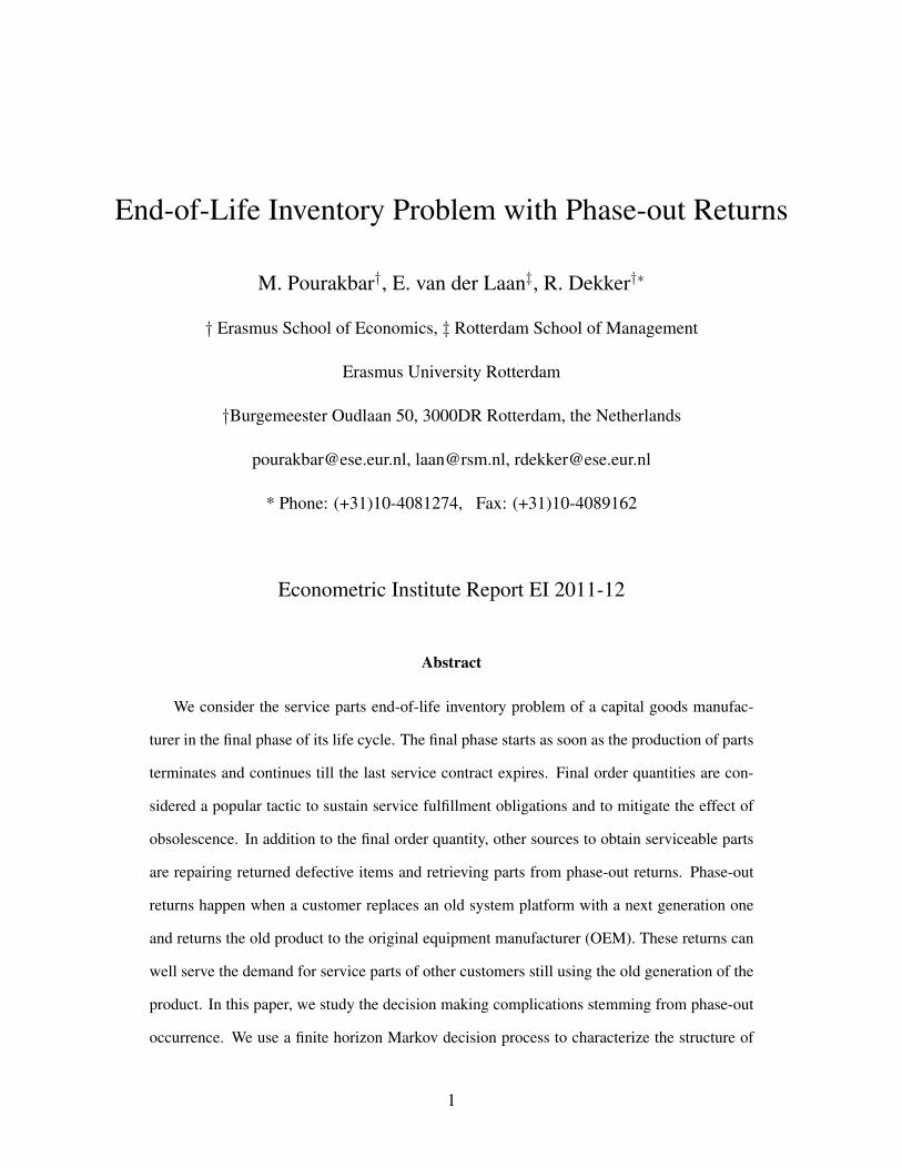
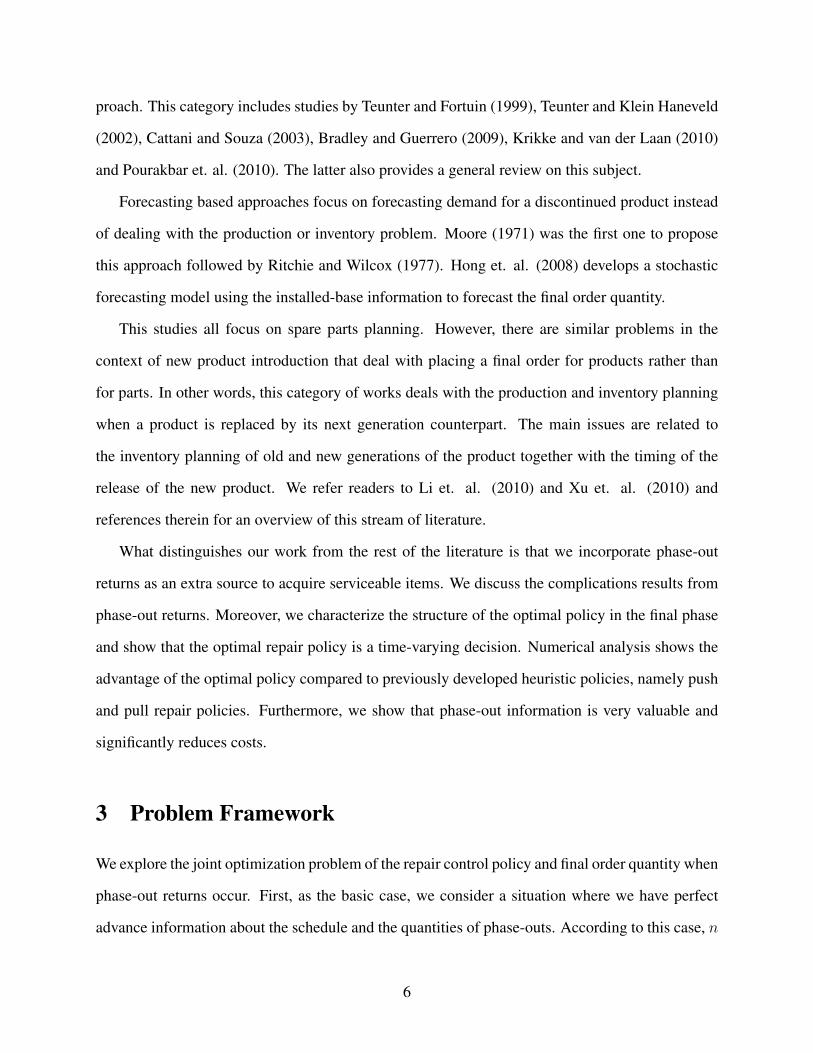
The system manager is interested in the effect of the phase-out schedule on the expected total
cost. Intuitively, it is not clear how postponing or pushing forward phase-out returns affects the
expected total cost. Thus, we carry out an analysis in which the quantity of the first phase-out
return is fixed, but the arrival schedule is varied over time. As can be observed in figures 5 and 6,
there is an optimal time to receive phase-out items. The corresponding diagram shows the effect of
the phase-out schedule on the expected total cost for different quantities of the phase-out returns.
When the phase-out quantity increases, the system first prefers to postpone the arrival of phase-out
returns. However, when a large quantity of phase-out returns are planned to arrive the optimal
schedule will push forward to the beginning of the horizon (figure 6). Furthermore, as we expect
intuitively increasing the phase-out quantity results in smaller final order quantities. These effects
are better represented in figure 7. As we observe for different values of cl, when the phase-out
quantities are very low or very high, the system prefers to receive them very early in time.
Therefore, when planning the inventory in the final phase, it is beneficial if the system manager
can plan the schedule of phase-out arrivals and force the customers to return phase-out returns in
the vicinity of the optimal schedule.
14
Page 15
0 20 40 60 806800
6900
7000
7100
7200
7300
7400
phase out arrival time
tota
l co
st
0 20 40 60 8040
42
44
46
48
50
52
54
56
58
phase out arrival time
fin
al o
rde
r q
ua
ntity
o1 = 7
o1 = 9
o1 = 12
Figure 5: Effect of phase-out schedule on expected total cost
0 20 40 60 805000
6000
7000
8000
9000
10000
11000
12000
phase out arrival time
tota
l co
st
0 20 40 60 800
10
20
30
40
50
60
phase out arrival time
fin
al o
rde
r q
ua
ntity
o1 = 30
o1 = 40
o1 = 50
Figure 6: Effect of phase-out schedule on expected total cost
15
Page 16
0 20 40 600
10
20
30
40
50
60
70
80
phase−out quantity
op
tim
al p
ha
se
−o
ut
sch
ed
ule
0 20 40 60 800
10
20
30
40
50
60
phase−out quantity
op
tim
al fin
al o
rde
r q
ua
ntity
cl = 500
cl = 1000
cl = 2000
Figure 7: Effect of phase-out quantity on optimal schedule and final order quantity
5 Numerical Analysis
In this section, we compare the performance of some heuristic policies already developed in the
literature for hybrid systems to the performance of the optimal policy for the general problem
described in section 4. Our aim is to assess the value of implementing the optimal policy instead
of simpler heuristics. We focus on heuristics that involve fixed (non-state dependent) parameters,
since they are simpler to communicate and implement and, perhaps, are more common in practice.
Below we provide a description of each of the heuristics we consider.
5.1 Heuristic 1: Push Policy
Under heuristic 1, in each period t, if there is repairable item the system triggers repair or in other
words the repairable items are immediately sent to repair shop as soon as they arrive. In this case
16
Page 17
the optimality equation where x ≥ 1 and y ≥ 1 can be expressed as
ν11(t, x, y) = (1− λ(t))µ{hs(x+ 1) + hr(y − 1) + cr + αν(t+ 1, x+ ot+1 + 1, y − 1)}
+(1− q)λ(t)µ {hsx+ hr(y + 1) + cr + αν(t+ 1, x+ ot+1, y − 1)}
+qλ(t)µ{hsx+ hry + cr + αν(t+ 1, x+ ot+1, y)
}+(1− λ(t))(1− µ){hsx+ hry + αν(t+ 1, x+ ot+1, y)}
+(1− q)λ(t)(1− µ){hs(x− 1) + hry + αν(t+ 1, x+ ot+1 − 1, y)}
+qλ(t)(1− µ){hs(x− 1) + hr(y + 1) + αν(t+ 1, x+ ot+1 − 1, y + 1)}(10)
Relations 4-6 need to be modified based on this policy similar to (10).
5.2 Heuristic 2: Pull Policy with a Fixed Repair Threshold
In contrast to push, under heuristic 2 the system just repairs an item if the level of serviceable
inventory is below a ceratin threshold S. Relation (3) according to this policy is rewritten as
follows:
ν11(t, x, y) =
νp(t, x, y) 1 ≤ x ≤ S, y ≥ 1
νl(t, x, y) x > S, y ≥ 1(11)
If 1 ≤ x ≤ S, the system operates according to a push policy. Therefore, νp(t, x, y) can be
calculated according to a relation similar to relation (10). Moreover, where x > S, y ≥ 1 the
system does not trigger any repair operations and thus we have
νl(t, x, y) = (1− λ(t)){hsx+ hry + αν(t+ 1, x+ ot+1, y)
}+(1− q)λ(t)
{hs(x− 1) + hry + αν(t+ 1, x+ ot+1 − 1, y)
}+qλ(t)
{hs(x− 1) + hr(y + 1) + αν(t+ 1, x+ ot+1 − 1, y + 1)
} (12)
17
Page 18
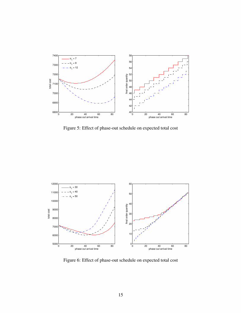
5.3 Experimental Design
In our numerical test, the planning horizon is 200 periods, i.e. H = 200. We assume that there
are three planned phase-outs arriving at times 30, 85 and 145 with a size of 7, 4 and 9 respectively.
The demand arrival rates are set at 0.9, 0.7, 0.4 and 0.2 respectively between each two consecutive
phase-out returns. The other system parameters are chosen from the following sets, which generate
a total of 64 different combinations. Sets are as follows µ ∈ {0.3, 0.8}, q0 ∈ {0.1, 0.7}, cl ∈
{1000, 2500}, cr ∈ {25, 125}, css ∈ {40, 120}, hs ∈ {0.5, 1.5}, hr = 0.5 and csr = 40.
We compute the cost and final order quantity for each instance with different parameters under
optimal and heuristic policies. We report the average, minimum and maximum cost increase re-
sulting from each heuristic policy compared to the optimal policy. We define the cost increase by
the following expression
∆cost =TCh − TCopt
TCopt× 100%
where, TCh and TCopt are expected cost according to heuristic and optimal policies, respectively.
The numerical results in table 1 show that on average the pull policy outperforms the push pol-
icy, as intuition might dictate. This is because while repair is triggered according to a push policy,
the system does not utilize any information regarding time and state of the system. However, the
pull policy benefits from deliberately postponing the repair operation. The average cost increase
for a pull policy is 6.83% compared to 20.75% for a push policy. Moreover, in some cases im-
plementing a push or pull policy instead of an optimal policy can impair the performance of the
system as much as 43.68% or 31.10%, respectively. Moreover, on average the pull policy tends to
place a larger final order quantity than the optimal policy, whereas push always places a smaller
final order quantity. This can be easily justified considering the structure of each policy. Basically,
the system expects to yield more serviceable items through repair when it operates according to
a push rather than a pull policy. Therefore, the final order quantity is smaller when the repair
operation is controlled according to a push structure.
18
Page 19
Table 1: The Value of the Optimal Policy
∆cost% Max ∆cost% Min ∆cost%Push 20.75 43.68 3.70Pull 6.83 31.10 0.35
Table 2: Final order quantity
Average n Max n Min nOptimal 61.76 83 39
Push 59.78 82 37Pull 64.75 85 42
5.4 Impact of Cost Terms
In this section, we first aim at exploring the impact of various cost parameters on the value of
the optimal control policy and secondly at understanding better the performance of push and pull
policies. To achieve this, we assign different values to a specific parameter and keep other variables
constant. For the base case scenario the parameters are set as shown in table 1. Figure 8 suggests
that there are many situations for which a push might outperform a pull policy. Figure 8.a implies
that as the holding cost for repairable items increases, the average error of a push policy decreases
whereas it increases for a pull policy. This is because it becomes more costly to hold repairable
items which makes push more appealing. Therefore, for larger values of hr push becomes superior
to pull. Moreover, as the serviceable item holding cost rate increases push becomes less attractive
and therefore pull outperforms push for larger hs, as shown in figure 8.b.
Next, we examine the impact of the repair rate on the value of the optimal policy (figure 8.c). As
the repair rate increases, pull tends to outperform push policy. This is because when the repair rate
is high, the repair operation becomes more reliable and therefore the system prefers to postpone the
Table 3: Base case parameters
cp cl cr hr hn csd crd q µ200 1000 75 0.5 1 80 40 0.3 0.4
19
Page 20
0.2 0.4 0.6 0.8 10
10
20
30
holding cost rate of repairable items
cost in
cre
ase (
%)
a.
0.5 1 1.5 2 2.50
5
10
15
20
25
holding cost rate of serviceable items
cost in
cre
ase (
%)
b.
0 0.2 0.4 0.6 0.80
5
10
15
20
25
repair rate
cost in
cre
ase (
%)
c.
20 40 60 80 100 120 1400
10
20
30
repair cost
cost in
cre
ase (
%)
d.
−200 −100 0 100 2000
10
20
30
40
disposal cost of serviceable items
cost in
cre
ase (
%)
e.
−100 −50 0 50 1000
10
20
30
40
disposal cost of repairable items
cost in
cre
ase (
%)
f.
500 1000 1500 2000 25000
10
20
30
lost sale cost
cost in
cre
ase (
%)
g.
Push Policy
Pull Policy
Figure 8: Impact of various parameters on the performance of heuristic policies
20
Page 21
repair operation and trigger it when the serviceable inventory hits a certain level. Since repairable
items are cheaper to hold, the system can benefit more from pull than push when repair can be
completed more swiftly. Furthermore, the increase in repair cost seems to impair the performance
of the push more than pull policy (figure 8.d). This is mainly due to the fact that pull can adjust S
in order to avoid extra repair cost.
As intuition dictates, push policy outperforms pull when the disposal of the serviceable item
generates a large revenue (figure 8.e). As the serviceable item disposal cost increases, push loses
its advantage and therefore pull tends to be a more effective policy. When it becomes more costly
to dispose of repairable items, then having less repairable stock at the end of the horizon becomes
more advantageous. Hence, we observe that the performance of the push policy improves when crd
increases (figure 8.f). Figure 8.g suggests that with the increase of the lost sale cost, both push and
pull policies impair performance significantly.
6 Extension to the Other Cases
Our model and approach can accommodate several related problems of interest as simple exten-
sions. In this section, we describe some of these cases. The main interest lies with phase-out
uncertainty. In practice, the phase-out arrival schedule is subject to considerable uncertainty. This
is because in order to switch from an old platform to a new one, the customer has to take many
sequential steps including purchasing, testing, personnel training etc. All of these activities are
subject to randomness that might render an uncertain phase-out arrival schedule. Furthermore, in
some cases, the OEM is not fully aware of the condition of platforms in use and therefore the
phase-out quantity is also subject to randomness. First, we extend the model to a case with phase-
out schedule uncertainty and then to a case with uncertain schedule as well as uncertain quantity.
21
Page 22
6.1 Phase-out Schedule is Stochastic While Quantities are Deterministic
In this case, the arrival of phase-out returns are subject to uncertainty, but we can limit the arrival
time, τi, to the interval [τ i, τ i] with arrival probability P{τi = t} = pi. In order to calculate the
policy cost, we define the function ω(τi, τi+1, x, y) as the cost function of running the policy from
time τi to τi+1. Therefore, the expected total cost function from time 0 to H is obtained by
Eω(x, y) =n∑i=0
τ i∑τi=τ i
τ i+1∑τi+1=τ i+1
pi(τi)pi+1(τi+1)ω(τi, τi+1, x, y) (13)
where τ0 = 0 and τn+1 = T . Moreover, ω(τi, τi+1, x, y) for τi ≤ t < τi+1 is defined as
ω(τi, t, x, y) =
ω11(τi, t, x, y) x ≥ 1, y ≥ 1
ω01(τi, t, x, y) x = 0, y ≥ 1
ω00(τi, t, x, y) x = 0, y = 0
ω10(τi, t, x, y) x ≥ 1, y = 0
(14)
which can be calculated in the same fashion as (3) and (4).
In order to investigate the effect of phase-out uncertainty, we limit our attention to the first
phase-out arrival and use the variance in the arrival schedule as a measure for uncertainty. As
intuition dictates, more variation around the optimal phase-out schedule results in a higher expected
total cost. The results are shown in figure 9. It is observed that the system places a larger final
order quantity in order to hedge against uncertainty when the coefficient of variation of the phase-
out schedule increases.
6.2 Both Phase-out Schedule and Quantities are Stochastic
In this situation, the quantity of phase-out returns is also subject to uncertainty. With probability
qi(k), k parts out of oi can immediately be added to the serviceable inventory and the rest should
22
Page 23
0 0.2 0.4 0.6 0.8 10
10
20
30
40
50
60
coefficient of variation of phase−out schedule
cost in
cre
ase (
%)
0 0.2 0.4 0.6 0.8 115
20
25
30
35
40
45
coefficient of variation of phase−out schedule
final ord
er
quantity
o1 = 40
o1 = 45
o1 = 50
Figure 9: Effect of phase-out arrival uncertainty on expected total cost
0 0.1 0.2 0.3 0.4 0.5 0.60
5
10
15
20
25
coefficient of variation of phase−out quantity
cost in
cre
ase (
%)
0 0.1 0.2 0.3 0.4 0.5 0.620
22
24
26
28
30
32
34
36
coefficient of variation of phase−out quantity
final ord
er
quantity
o1 = 40
o1 = 45
o1 =50
Figure 10: Effect of phase-out quantity uncertainty on expected total cost
undergo repairs. In this case, the expected total cost function from time 0 to H is obtained by
Eω(x, y) =n∑i=0
τ i∑τi=τ i
τ i+1∑τi+1=τ i+1
oi∑k=0
oi−k∑j=0
qi(k)pi(τi)pi+1(τi+1)ω(τi, t+ 1, x+ k, y + j) (15)
where ω(τi, t+ 1, x+ k, y + j) can be calculated similar to (14)
In order to investigate the effect of phase-out quantity uncertainty, we keep the standard de-
viation of the phase-out schedule at a fixed level and change the coefficient of variation of the
phase-out quantity while its expected value is fixed. The results are shown in figure 10. As can
be observed, more randomness in phase-out quantities results in an increase of final order quantity
23
Page 24
and consequently impairs the performance of the system.
7 Discussion and Conclusion
In this paper we address the end-of life inventory and repair planning for service parts in their final
phase. In particular, we focus on the final order quantity, taking into account product returns due
to failures and phase-outs and (optimal) repair policy.
When the schedule and quantities of phase-out returns are known in advance we proved that
the structure of the optimal policy is characterized in terms of state and time dependent threshold
levels r∗(t, y), where t is time and y is the remanufacturable inventory. So, whenever the level of
serviceable inventory x is below r∗(t, y), a part, if available, is sent to the repair shop.
Varying the arrival time of phase-outs, we see that there is an optimal timing of phase out
returns for a given phase-out quantity. When phase-out quantities are higher, the optimal timing
first moves later in time, but eventually moves earlier in time. Therefore, in constructing service
contracts it is important to take the timing of phase-outs into account or even negotiate optimal
timing.
The optimal policy combines push and pull in one policy. Simpler policies have previously
been developed and are widely used in practice, such as push (push repairable items upon arrival)
and pull (pull repairable items relative to a fixed serviceable inventory level). Our numerical study
suggests that push only outperforms pull when the holding cost rates for serviceable and reman-
ufacturable items are very close or when the repair rate is very small. The difference between
push and pull becomes smaller as the disposal cost for a remanufacturable part increases. For our
parameter setting, the optimal policy outperforms pull by up to 31.10% (6.83% on average). When
the serviceable holding cost rate or the probability that a part is remanufacturable is high, the per-
formance of pull is close to optimal. With respect to the final order quantity decision we see that
push always underestimates the optimal final order quantity, whereas pull always overestimates it.
Another finding highlight the vital importance of phase-out information. We show that un-
24
Page 25
certainties about the phase-out schedule and quantity can impair the performance of the system.
Having accurate information over phase-out returns can lead to considerable cost savings.
Even though the final phase is known as the longest phase of the service life cycle, it has
received little attention in the literature. Our work can be extended in various dimensions, for
instance, to a situation in which the OEM is allowed to dispose of inventories during the course of
the final phase. Another important extension is dealing with end-of-life inventory planning in the
presence of differentiated customers based on service contracts or equipment criticalness.
References
[1] Bradley J.R., H.H. Guerrero. 2009. Life-Time Buy Decisions with Multiple Parts, Production
and Operations Management, 18(1).
[2] Bulkeley W.M. . IBM. 1999. Had 98 PC pretax loss of nearly $ 1 billion, The Wall Street
Journal, March 25.
[3] Cattani K.D., G.C. Souza. 2003. Good buy? Delaying end-of-life purchases, European Jour-
nal of Operational Research, 146 216-228.
[4] Fortuin L. 1980. The All-Time Requirement of Spare Parts for Service After Sales- The-
oretical Analysis and Practical Results, International Journal of Operations and Production
Management, 1(1), 59-70.
[5] Fortuin L. 1981. Reduction of All-time requirements for Spare Parts, International Journal of
Operations and Production Management, 2(1), 29-37.
[6] Hong J.S., H.Y. Koo, C.S. Lee, J. Ahn. 2008. Forecasting service parts demand for a discon-
tinued product, IIE Transactions 40 640-649.
[7] Klein Haneveld W.K., R.H. Teunter. 1998. The Final Order Problem, European Journal of
Operational Research, 107 35-44.
25
Page 26
[8] Kooten J.P.J. van, T. Tan. 2009. The Final Order Problem for Repairable Spare Parts under
Condemnation. Journal of the Operational Research Society, 60 14491461.
[9] Krikke H.R., Laan E. van der. 2011. Last Time Buy and Control Policies With Phase-Out Re-
turns: A Case Study in Plant Control Systems, International Journal of Production Research.
[10] Li H, S.C. Graves, D.B. Rosenfield. 2010. Optimal Planning Quantities for Product Transition
, Production and Operations Management, 19(2) 142-155.
[11] Moore J.R. 1971. Forecasting and Scheduling for Past-Model Replacement Parts, Manage-
ment Science 18 B200-B213.
[12] Teunter R.H., L. Fortuin. 1998. End-of-life service: A case study, European Journal of Oper-
ational Research, 107 19-34.
[13] Teunter R.H., W.K. Klein Haneveld. 2002. Inventory control of service parts in the final
phase, European Journal of Operational Research 137 497-511.
[14] Pourakbar M., J.B.G. Frenk, R. Dekker. 2010. End-of-life inventory decisions for consumer
electronics service parts, econometric institute report series, Erasmus University Rotterdam.
[15] Ritchie E., P.Wilcox. 1977. Renewal Theory Forecasting for Stock Control, Jornal of the
Operational Research Society, 1 90-93.
APPENDIX
Proof of Lemma 1
Proof. First, for the sake of brevity we define ξ(t, x, y) = ν11(t, x, y) − ν11(t, x − 1, y). Then,
we need to show that ξ(t, x, y) is non-decreasing in x. Moreover, we define ξ(t, 0, y) = α/cl. We
follow an induction approach in order to show the desired results.
From the terminal value definition we have ν11(H, x, y) = csdx + crdy, thus, ξ(H, x, y) = csd.
From assumption (1) we have cl ≥ αcsd which can be immediately translated to ξ(H, 1, y) ≥
ξ(H, 0, y). Therefore, ξ(H, x, y) is non-decreasing in x.
26
Page 27
Following the induction, we assume ξ(t−1, x, y) is non-decreasing in x, then we need to show
that ξ(t, x, y) is non-decreasing in x. From the definition of r∗(t, y) we know that there exists a
r∗(t, y) such that if x ≥ r∗(t, y) then it is optimal not to repair and repair otherwise. It is worth
nothing that λ(t) = λ for t ∈ [τi, τi+1). Then from equation (3) we have
ξ(t− 1, x, y) =
(1− λ){hs + αξ(t, x, y)1{x≥r∗(t,y)}}
+(1− q)λ{hs + αξ(t, x− 1, y)1{x−1≥r∗(t,y)}}
+qλ{hs + αξ(t, x− 1, y + 1)1{x−1≥r∗(t,y+1)}}
+(1− λ){hs + (1− µ)αξ(t, x, y)1{x<r∗(t,y)} + µ(αξ(t, x+ 1, y − 1) + cr)1{x<r∗(t,y)}}
+(1− q)λ{hs(1− µ)αξ(t, x− 1, y)1{x−1<r∗(t,y)} + µ(αξ(t, x, y − 1) + cr)1{x−1<r∗(t,y)}}
+qλ{hs + (1− µ)αξ(t, x− 1, y + 1)1{x−1<r∗(t,y+1)} + µ(αξ(t, x, y) + cr)1{x−1<r∗(t,y)}}
since ξ(t−1, x, y) is a linear expression of ξ(t, x, y) and using induction assumption we know that
ξ(t− 1, x, y) is non-decreasing in x therefore ξ(t− 1, x, y) is non-decreasing in x. The same can
be established for expressions (6), (8) and (10).
Using the same approach and the fact that hs ≥ hr we can show that ξ(t, x, y) is non-decreasing
in y. �
Proof of Theorem 2
I. The results are intuitive considering the definition of the repair threshold and component-
wise convexity properties.
II.
Proof. We show this by induction where the induction assumption is r∗(t, y) ≤ r∗(t − 1, y) and
β(t−1, x, y) ≥ β(t, x, y), where β(t, x, y) = ν11(t, x+1, y−1)−ν11(t, x, y). It is straightforward
27
Page 28
to show the results for t = H , since intuitively r∗(H, y) = 0 ≤ r∗(H − 1, y).
Then, assuming the induction assumption holds at time t − 1 we need to show that it holds at
time t. In order to show that the induction assumption holds we employ a contradiction approach.
Suppose for contradiction that r∗(t − 1, y) < r∗(t, y). Using the definition of repair threshold it
immediately implies that β(t, r∗(t− 1, y), y) + cr ≥ 0. Using (3), we should note that
β(t− 1, x, y) = (1− λ){αβ(t, x, y)1{x≥r∗(t,y)}}
+(1− q)λ{αβ(t, x− 1, y)1{x−1≥r∗(t,y)}}
+qλ{αβ(t, x− 1, y + 1)1{x−1≥r∗(t,y+1)}}
+(1− λ){(1− µ)αβ(t, x, y)1{x<r∗(t,y)} + µαβ(t, x+ 1, y − 1)1{x<r∗(t,y)}}
+(1− q)λ{(1− µ)αβ(t, x− 1, y)1{x−1<r∗(t,y)} + µαβ(t, x, y − 1)1{x−1<r∗(t,y)}}
+qλ{(1− µ)αβ(t, x− 1, y + 1)1{x−1<r∗(t,y+1)} + µαβ(t, x, y)1{x−1<r∗(t,y)}}
For the ease of representation we define ∆tβ(t, x, y) = β(t, x, y) − β(t + 1, x, y), Then we
28
Page 29
have∆tβ(t− 1, r∗(t, y), y) = (1− λ){α∆tβ(t, r∗(t, y), y)1{r∗(t,y)≥r∗(t+1,y)}}
+(1− q)λ{α∆tβ(t, r∗(t, y)− 1, y)1{r∗(t,y)−1≥r∗(t+1,y)}}
+qλ{α∆tβ(t, r∗(t, y)− 1, y + 1)1{r∗(t,y+1)−1≥r∗(t+1,y+1)}}
+(1− λ){(1− µ)α∆tβ(t, r∗(t, y), y)1{r∗(t,y)<r∗(t+1,y)}}
+(1− λ)µα∆tβ(t, r∗(t, y) + 1, y − 1)1{r∗(t,y)<r∗(t+1,y)}
+(1− q)λ{(1− µ)α∆tβ(t, r∗(t, y)− 1, y)1{r∗(t,y)−1<r∗(t+1,y)}}
+(1− q)λµα∆tβ(t, r∗(t, y), y − 1)1{r∗(t,y)−1<r∗(t+1,y)}
+qλ{(1− µ)α∆tβ(t, r∗(t, y)− 1, y + 1)1{r∗(t,y+1)−1<r∗(t+1,y+1)}}
+qλµα∆tβ(t, r∗(t, y), y)1{r∗(t,y)−1<r∗(t+1,y)}
Using the induction assumption, we have the terms ∆tβ(t, x − 1, y + 1), ∆tβ(t, x − 1, y) and
∆tβ(t, x, y) are all non-negative. Therefore, ∆tβ(t − 1, x, y) = β(t − 1, x, y) − β(t, x, y) ≥ 0.
Thus,
β(t− 1, x, y) + cr ≥ β(t, x, y) + cr ≥ 0
which implies that r∗(t, y) ≤ r∗(t− 1, y), it is a contradiction.
Next, we show β(t − 1, x, y) ≥ β(t, x, y) given that r∗(t, y) ≤ r∗(t − 1, y), t ∈ (0, H].
We separate the interval (0, r∗(t − 1, y)] into the following subintervals (0, r∗(t + 1, y)], (r∗(t +
1, y), r∗(t, y)] and (r∗(t, y), r∗(t−1, y)]. For each of these intervals we show the results. It is worth
mentioning that we use the notation ∆tβ(t, x, y) as defined previously. Moreover, we just show
the results for the case that x ≥ 1 and y ≥ 1, a similar analysis can be applied to other cases.
Case 1. ∀x ∈ (0, r∗(t+ 1, y)]
29
Page 30
In this case we have
∆tβ(t− 1, x, y) =
(1− λ){(1− µ)∆tβ(t, x, y)1{r∗(t,y)<r∗(t+1,y)} + µ∆tβ(t, x+ 1, y − 1)1{r∗(t,y)<r∗(t+1,y)}}
+(1− q)λ{(1− µ)∆tβ(t, x− 1, y)1{r∗(t,y)−1<r∗(t+1,y)} + µ∆tβ(t, x, y − 1)1{r∗(t,y)−1<r∗(t+1,y)}}
+qλ{(1− µ)∆tβ(t, x− 1, y + 1)1{r∗(t,y+1)−1<r∗(t+1,y+1)} + µ∆tβ(t, x, y)1{r∗(t,y)−1<r∗(t+1,y)}}
Following an approach similar to the previous case we can show that the right hand side are all
non-negative and therefore ∆tβ(t− 1, x, y) ≥ 0.
Case 2. ∀x ∈ (r∗(t+ 1, y), r∗(t, y)]
∆tβ(t− 1, x, y) = (1− λ){∆tβ(t, x, y)1{r∗(t,y)≥r∗(t+1,y)}}
+(1− q)λ{∆tβ(t, x− 1, y)1{r∗(t,y)−1≥r∗(t+1,y)}}
+qλ{∆tβ(t, x− 1, y + 1)1{r∗(t,y+1)−1≥r∗(t+1,y+1)}}
Following an approach similar to the previous case we can show that the right hand side are all
non-negative and therefore ∆tβ(t− 1, x, y) ≥ 0.
Case 3. ∀x ∈ (r∗(t, y), r∗(t− 1, y)]
In this case we have r∗(t, y) < x ≤ r∗(t− 1, y), then according to the definition of r∗(t, y) we
have β(t− 1, x, y) + cr ≥ 0 and β(t, x, y) + cr ≤ 0 therefore β(t− 1, x, y)− β(t, x, y) ≥ 0.
These show the desired results for x ≥ 1 and y ≥ 1. We can follow a similar approach for
other cases. �
30