End of Training Project Report - UCLouvain of Training Project Report September10, 2008 Patterns and...

End of Training Project

Report

September 10, 2008

Patterns and causes of sea-ice variability in the decadal

ECCO-GODAE (version 3) coupled ocean/sea-ice state estimate

Olivier Lecomte

ENSI08 - HY

Patterns and causes of sea-ice variability in the decadal

ECCO-GODAE (version 3) coupled ocean/sea-ice state estimate

Program of Atmospheres, Oceans, and Climate, Department of

Earth, Atmospheric and Planetary Sciences,

Massachusetts Institute of Technology, Cambridge, Massachusetts

Supervisors:

Patrick Heimbach, Department of Earth and Atmospheric Science,

MIT Building 54, Room 1518, 77 Massachusetts Avenue, Cambridge, MA, 02139

E-mail: [email protected]

Carl Wunsch, Department of Earth and Atmospheric Science,

MIT Building 54, Room 1518, 77 Massachusetts Avenue, Cambridge, MA, 02139

E-mail: [email protected]

2

Contents

1 Introduction 5

2 Sea ice concentration fields – a first description 7

2.1 Observations from passive microwave radiometry vs. Estimates from ECCO-GODAE, v3.35 7

2.2 Cost/misfit calculations . . . . . . . . . . . . . . . . . . . . . . . . . . . . . . . . . . . . . 15

3 Sea ice concentration variability 17

3.1 Inter-annual Southern Ocean components . . . . . . . . . . . . . . . . . . . . . . . . . . . 17

3.2 Sector correlations . . . . . . . . . . . . . . . . . . . . . . . . . . . . . . . . . . . . . . . . 21

4 Atmospheric mechanisms 23

5 Oceanic mechanisms 26

5.1 Trends over the 15 years . . . . . . . . . . . . . . . . . . . . . . . . . . . . . . . . . . . . . 26

5.2 EOF Analyses . . . . . . . . . . . . . . . . . . . . . . . . . . . . . . . . . . . . . . . . . . . 29

5.2.1 Sea Surface Temperature . . . . . . . . . . . . . . . . . . . . . . . . . . . . . . . . 29

5.2.2 Sea Surface Salinity . . . . . . . . . . . . . . . . . . . . . . . . . . . . . . . . . . . 31

5.2.3 Mixed-Layer Depth . . . . . . . . . . . . . . . . . . . . . . . . . . . . . . . . . . . . 33

5.3 Correlation Analyses . . . . . . . . . . . . . . . . . . . . . . . . . . . . . . . . . . . . . . . 34

6 Conclusions 36

A EOF/PCA and SVD analysis of Climatic Data 38

A.1 What is it all about and when to use each method . . . . . . . . . . . . . . . . . . . . . . 38

A.2 The Data . . . . . . . . . . . . . . . . . . . . . . . . . . . . . . . . . . . . . . . . . . . . . 39

A.3 How to do it . . . . . . . . . . . . . . . . . . . . . . . . . . . . . . . . . . . . . . . . . . . 40

A.3.1 Principle . . . . . . . . . . . . . . . . . . . . . . . . . . . . . . . . . . . . . . . . . 40

3

CONTENTS

A.3.2 How to compute it . . . . . . . . . . . . . . . . . . . . . . . . . . . . . . . . . . . . 41

A.3.3 How to understand it physically . . . . . . . . . . . . . . . . . . . . . . . . . . . . 43

A.3.4 SVD of coupled fields . . . . . . . . . . . . . . . . . . . . . . . . . . . . . . . . . . 43

B Dates of Minimum and Maximum SIC 45

C AAO, SOI and Nino-3 Indices 46

D EOFs calculation MATLAB code 48

4

Chapter 1

Introduction

While the decline of Arctic sea-ice cover over the last two decades has been the subject of much media

attention (2007 marked the lowest coverage since the beginning of the combined SMMR/SSMI satellite

record1, Serreze et al. (2007)), a fundamentally different behaviour of the Southern Ocean (SO) sea-ice

cover has received little notice. Recent estimates of SO sea-ice concentration changes report a weak

upward trend in SO sea-ice concentration of 0.21 ± 0.12 106 km2/decade for the period 1979 to 2004

(e.g. Zwally et al. (2002); Kwok and Comiso (2002); Cavalieri and Parkinson (2008)). In fact the austral

summer of 2007/08 satellite observations reveal the highest Antarctic summer sea-ice extent since 1979).

SO sea-ice concentration exhibits a strong seasonal cycle with little perennial ice surviving from

one year to the next as sea-ice retreats during austral summer, it also exhibits significant interannual

variability. At the same time, regional analyses in the Weddell, Indian, Pacific, Ross, Amundsen, and

Bellinghausen sectors reveal strong regional variability with significant differences in character from

sector to sector. So despite previous work indicating an upward trend, there are large uncertainties on

current trend estimates because of seasonal and regional variability.

The nature and cause of regional variability of SO sea-ice concentration remains very much an open re-

search question. Various groups have analyzed (i) co-variability between different sectors around Antarc-

tica, as well as (ii) linkages between sea ice concentration anomalies and climate indices. With regard

to (i), two views dominate current thinking. One is the existence of a so-called Antarctic Circumpolar

Wave (ACW) which travels around Antarctica with an 8 to 10 year period, (e.g. White and Peterson

(1996)). The second focuses on an Antarctic Dipole (AD), a seesaw between Weddell and Amundsen

sector sea ice concentration anomalies, (cf. Yuan and Martinson (2000); Holland et al. (2005)). With

1Scanning Multichannel Microwave Radiometer (SMMR) and Special Sensor Microwave Imager (SSMI) satellites provideinformation on the global sea ice cover from 1978 to present in 1978.

5

CHAPTER 1. INTRODUCTION

regard to (ii), among the most studied atmospheric teleconnections linking Antarctic sea-ice anomalies

to climate indices are the Antarctic Oscillation, AAO (or Southern Annular Mode, SAM), as well as

ENSO-related indices such as the Southern Oscillation Index (SOI), and the Nino-3 index, (Carleton

(2003); Liu et al. (2004)). While such teleconnections are clearly corroborated by these studies, it seems

these by themselves cannot explain the bulk of of Antarctic sea-ice variability, in particular its regional

trend patterns.

Compared to the above analyses the role of the ocean has been little studied, probably in part due

to the lack of continuous observations in large parts of the SO. Here we use results from a new version

of the Estimating the Circulation and Climate of the Ocean – Global Ocean Data Assimilation (ECCO-

GODAE) effort. It is based on a dynamically consistent quasi-global coupled ocean-sea-ice state that has

been forced to most of the oceanic observations available since the early 1990s, such as satellite altimetry,

a GRACE-based mean dynamic topography, Reynolds SST fields, Argo profiling floats, CTD casts and

XBT observations from the WOCE program and many others (for a more comprehensive summary see

e.g. Wunsch and Heimbach (2007)).

Sea-ice observations have not been used to constrain the sea-ice component. The estimated sea

ice state needs special scrutiny which is a first step in our planned analyses. Its misfit to the combined

SMMR/SSMI sea-ice concentration fields obtained from the National Snow and Ice Data Center (NSIDC)

and retrieved via an updated version of the so-called ”Bootstrap algorithm”2 will be assessed for the

years 1992-2006 spanning the state estimate.

Thus, we will start by studying both data sets (observations and model data) in order to give a good

description of the Sea-Ice Concentration (SIC) fields, of their over-all trends and of the misfit between the

ECCO estimate and the satellite records. Our investigation will then follow along two routes. On the one

hand we will use climate indices available from the NOAA Climate Prediction Center (NOAA/CPC) to

infer regional patterns of co-variability between sea-ice anomalies and those indices in the spirit of earlier

studies. On the other hand we will take full advantage of the estimated ECCO-GODAE ocean state to

explore the role of the ocean. Near-surface properties such as upper ocean heat content, near-surface

salinity, mixed layer depths will receive special attention, as they provide the most immediate link to

sea-ice thermodynamical properties. Using a combination of statistical tools (EOF, SVD, CCA analyses)

and physical insights underlying Southern Ocean dynamics and thermodynamics, we will explore the role

of the ocean in driving Antarctic sea-ice concentration changes.2The bootstrap technique as described by Comiso (1986) and Comiso and Sullivan (1986) uses basic radiative transfer

equations and takes advantage of unique multichannel distributions of sea ice emissivity.

6

Chapter 2

Sea ice concentration fields – a first

description

2.1 Observations from passive microwave radiometry vs. Esti-

mates from ECCO-GODAE, v3.35

National Snow and Ice Data Center (NSIDC) provides with daily sea-ice concentration fields from January

1, 1992 to December 31, 2007 (obtained by satellite observation). However within the context of the

comparison of the observations with ECCO-GODAE output data, we will stop the study to the end of

2006 as there are no model data for 2007 at the time of writing. Observations for 2007 can be analysed

separately. The purpose of this first part is to display the data in a readable way in order to study

the sea-ice coverage evolution over the 15 years. NSIDC gives sea-ice concentration fields for the whole

ocean, plus the land-ice ones. So the first step consists in multiplying the ice concentration field by the

land mask (to keep the sea-ice coverage only) and displaying the Southern Ocean area of interest, below

latitude 50S. It is also interesting to display the different sectors of the Southern Ocean (Weddell sea,

Indian sector, Pacific sector, Amundsen sector, Bellingshausen sector and Ross sea) for the purpose of

further correlation studies.

7

CHAPTER 2. SEA ICE CONCENTRATION FIELDS – A FIRST DESCRIPTION

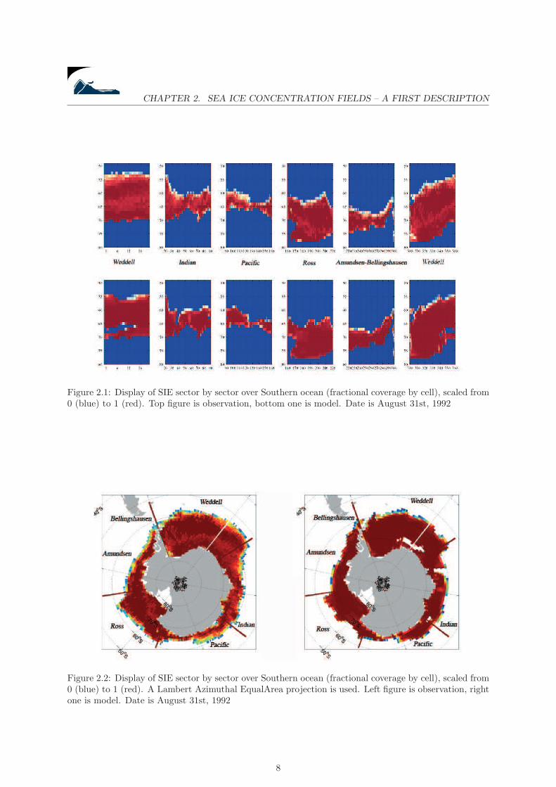
Figure 2.1: Display of SIE sector by sector over Southern ocean (fractional coverage by cell), scaled from0 (blue) to 1 (red). Top figure is observation, bottom one is model. Date is August 31st, 1992

Figure 2.2: Display of SIE sector by sector over Southern ocean (fractional coverage by cell), scaled from0 (blue) to 1 (red). A Lambert Azimuthal EqualArea projection is used. Left figure is observation, rightone is model. Date is August 31st, 1992

8


We get a better quality of display when using a map projection tool (using Lambert Azimuthal

EqualArea but non conform projection). See figure 2.1 and 2.2 as examples.

The same kind of data is produced by the ECCO Model, so that we can apply the same process to the

output data and compare the results by plotting the sea-ice coverage for both model data and satellite

observations. Thus the time series of area-integrated ice concentration were computed and displayed

as movies showing the annual ice melting and forming cycle for every year from 1992 to 2006. Figures

2.3 shows the Southern-Ocean sea ice coverage evolution over 1992. These figures illustrate quite well

the seasonal cycle in four steps. Months of minimum and maximum coverage are respectively February

and September like it is almost for every year (exact months of minimum/maximum concentration were

determined from the sea ice integrated area signal and are displayed in the tab, appendix B), which is

consistent with Parkinson (2004); Cavalieri and Parkinson (2008). The first thing to notice (see figure

2.3) is that the model clearly underestimates the observations during austral summer. This implies that

sea ice will melt faster than in observations. Also If one looks at the SIC maps of September 1992 (figure

2.3.c), a pronounced polynia in the form of a hole in sea ice concentration in the Weddell Sea is apparent

which seems to point to an artifact in the model (right panel). Therefore when the misfit between

observations and model will be computed, large values of the error should show up in the corresponding

areas, if the anomalies are recurrent (when watching the SIC maps movies we see that indeed they are).

9


(a) February 1992

(b) June 1992

(c) September 1992

(d) December 1992

Figure 2.3: Sea-Ice coverage (monthly averaged) for both observations (left) and model (right).

10


For each year, the monthly averaged ice concentration was calculated (to set the data free of non-

relevant daily noise), and expressed both in square meters and in fractional area of the globe. Indeed the

ice coverage can be derived from the model output by summing the coverage (sea ice concentration in

each model grid-cell multiplied by the cell area) over the whole grid. Then by comparison with the area

of the entire grid (i.e. part of the global grid restricted to Southern Ocean) we get the fractional area of

the globe that ice covers. Figure 2.4 presents the sea-ice area integrated over the whole Southern-Ocean

along year 1992 for both observations and model data. Figure 2.5 is the same plot but extended to the

15-year period with the linear regressions associated with each curve that give a general trend for sea-ice

extent over the 15 years.

0 2 4 6 8 10 120

2

4

6

8

10

12

14

16x 10

12

Figure 2.4: Sea ice area variation along year 1992 (in m2). Blue curve represents the observations andred one corresponds to the model. X-axis in months.

0 20 40 60 80 100 120 140 160 1800

2

4

6

8

10

12

14

16x 10

12

Figure 2.5: Sea ice area variation along the 15 years sample, from 1992 to 2006 (in m2). Blue curverepresents the observations and red one corresponds to the model. X-axis in months.

11


From these two figures we clearly identify the seasonal cycle. On the maps of the time series of the

raw data we could see that the model underestmates SIC during summer, now we see that in terms of

integrated area the model ( always) underestimate the observations. This is what the shift between the

two curves suggests. Also, the linear regressions performed on both plots give the following results:

Observation trend = 4.8232.109 m2/mth, Linear regression initial value = 8.4110.1012 m2

Model trend = -7.2907.108 m2/mth, Linear regression initial value = 6.7679.1012 m2

Thus, in addition to the noticeable shift between the curves there is an inconsistancy regarding the sign

of the trends. What will subsequently be interesting to do is to check if this inconsistancy persists when

the seasonal cycle is filtered out.

It is also necessary to remove the seasonal cycle to get a significant information regarding sea ice

inter-annual variability. In order to do this and to look at the decadal tendencies, two methods have

been implemented. The first one, which follows Fourier analysis principle, consists in fitting the data

with a periodic signal like sine and/or cosine to extract the seasonal variation of SIC. Let us assume that

this seasonal signal is close to the following:

f(x) = a0 + a1 cos(xw) + b1 sin(xw) (2.1)

where f would be either the sea ice area or the fractional coverage, x the months and w the frequency

of the seasonal cycle. Then performing the non-linear regression (based on dichotomia) of the data with

this function we find the coefficients a0, a1 and b1. The results are presented in figures 2.6 and 2.7.

We find values equal to 0.5232 and 0.5234 for w respectively for observations and model data. Now by

definition:

w = 2 π/T (2.2)

where T is the seasonal cycle period (in month). With such values for w, we find periods about 12

months as expected.

Once we get this seasonal signal characterized by the latter formula, we remove it from the whole

signal and perform a simple linear regression on the residual (figure 2.8). However one can notice that

a 12 months variability remains in the residual, for the reason that we only retain the first harmonic in

the Fourier decomposition of the signal, so its annual variability has not been entirely removed. Further

in this study we compute the EOFs decomposition of the SIC time series, that is why we need to remove

most of the seasonal signal so that it is not the dominant signal in the different EOF modes (in other

12


words, to be able to see other modes of variability than the seasonal one). Thus, althougt this analysis

gives us a more precise idea of the sesonal cycle, it is not satisfactory. An other way to remove the annual

cycle is to run a 12-months running average on the data. This has been done in figure 2.9. On these

pictures we also see the linear regression performed on the residual signal. In this case it seems the main

part of the seasonal variability has disappeared. A summary of the standard deviations and trends from

the different linear regressions is given in the following tables.

Obs./Fourier Residual Obs./12mths running mean

Trend from linear regression (m2/mth) 4.5550 108 1.4192 109

Std of ’Residual-Regression’ (m2) 9.2529 1011 2.2769 1011

Mod./Fourier Residual Mod./12mths running mean

Trend from linear regression (m2/mth) -5.2498 109 -4.2392 109

Std of ’Residual-Regression’ (m2) 1.2777 1012 2.5384 1011

The two methods give consistant results one with each other (trends have different amplitudes but

the same sign). However, similarly to raw data, filtered model data suggest a different global tendency

(decreasing integrated SIC anomaly) from the one of the observations (increasing). That means the ice

extent in the model is decreasing over the 15 years, while observations indicate the opposite (which is

qualitatively consistent with trends published by other groups, Parkinson (2004); Cavalieri and Parkinson

(2008), although they are quantitatively different since they are calculated on a different spanning time).

Thus the inconsistancy noticed while performing linear regressions on raw data is still observable when

the annual cycle is removed, which means it is not an artifact coming from the period of calculation of

the trend but a real discrepency between observations and model.

13


0 20 40 60 80 100 120 140 160 180

2

4

6

8

10

12

14

16x 10

12

Figure 2.6: Non-linear regression of theobservations with fourier function. a0=8.8581012m2, a1=-2.037 1012m2, b1=-6.6311012m2,w=0.5234. X-axis in months, Y-axisin m2.

0 20 40 60 80 100 120 140 160 180

0

2

4

6

8

10

12

14

16x 10

12

Figure 2.7: Non-linear regression of the Modeldata with fourier function. a0=6.786 1012m2,a1=-2.882 1012m2, b1=-7.142 1012m2,w=0.5232. X-axis in months, Y-axis in m2.

0 20 40 60 80 100 120 140 160 180−2.5

−2

−1.5

−1

−0.5

0

0.5

1

1.5

2x 10

12

0 20 40 60 80 100 120 140 160 180−4

−3

−2

−1

0

1

2

3x 10

12

Figure 2.8: Fourier Residual (Obs.-Regression for left figure and Mod.-Regression for right figure) andlinear regression of the residual. X-axis in months, Y-axis in m2.

0 20 40 60 80 100 120 140 160 1808.3

8.4

8.5

8.6

8.7

8.8

8.9

9

9.1

9.2

9.3x 10

12

0 20 40 60 80 100 120 140 160 1805.8

6

6.2

6.4

6.6

6.8

7

7.2

7.4x 10

12

Figure 2.9: 12-months running mean applied to SIC integrated area and linear regression of these signals.Left figure is observations, right figure is model. X-axis in months, Y-axis in m2.

14


2.2 Cost/misfit calculations

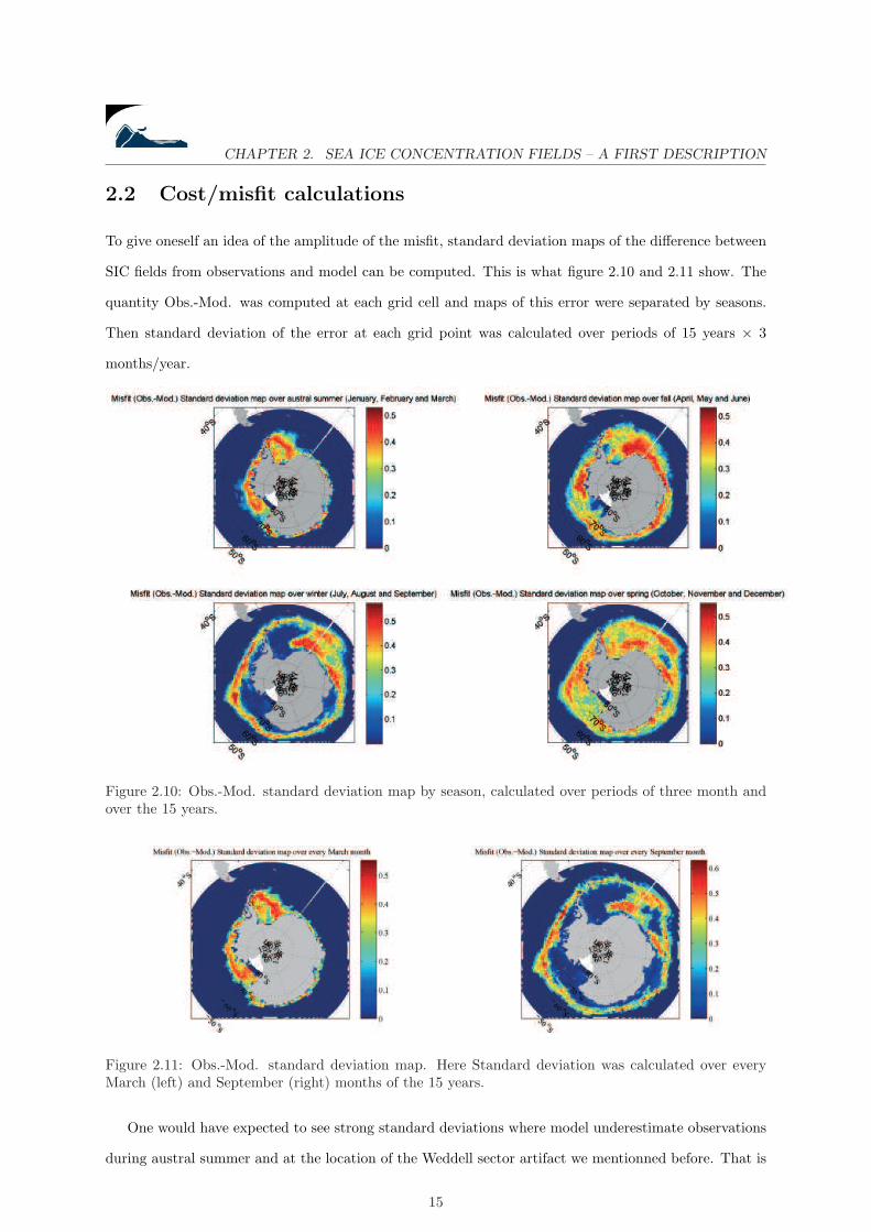
To give oneself an idea of the amplitude of the misfit, standard deviation maps of the difference between

SIC fields from observations and model can be computed. This is what figure 2.10 and 2.11 show. The

quantity Obs.-Mod. was computed at each grid cell and maps of this error were separated by seasons.

Then standard deviation of the error at each grid point was calculated over periods of 15 years × 3

months/year.

Figure 2.10: Obs.-Mod. standard deviation map by season, calculated over periods of three month andover the 15 years.

Figure 2.11: Obs.-Mod. standard deviation map. Here Standard deviation was calculated over everyMarch (left) and September (right) months of the 15 years.

One would have expected to see strong standard deviations where model underestimate observations

during austral summer and at the location of the Weddell sector artifact we mentionned before. That is

15


indeed what happens if we look at winter and summer maps, but there is something else to notice. Strong

values of standard deviation show up in the Southern Ocean periphery during austral winter periods.

Now studying sea ice state, we can speak in terms of concentration (SIC), thickness (characterizing sea

ice vertical state and growth), integrated area or even Sea Ice Edge (SIE, characterizing meridional sea

ice state and growth). Well the previous remark suggest that the model underestimate the SIE too.

However, very weak stantard deviations of the misfit can be noticed in some more inner parts of the

southern ocean; which is a good point to study and understand why the sea ice state estimate is quite

good in these areas and especially why the estimate is not as good elsewhere.

16

Chapter 3

Sea ice concentration variability

3.1 Inter-annual Southern Ocean components

To describe SIE variability, an Empirical Orthogonal Function (EOF) analysis (see appendix A) was per-

formed on the data (both observations and model data). First, to remove the ”intra-annual” variability,

a 12-months running mean was applied to every grid point of the field prior to the EOF analysis. Then

as usual for EOF compuations, the data was centered (mean over the 15 years was removed from it so

that we analyse an anomaly). The covariance matrix of the data was computed as its eigenvectors (via

singular value decomposition) which are also the so-called EOF ”components” or ”modes”. The follow-

ing figures present these patterns with the associated ”time-series” or ”expansion coefficients”. The first

EOF pattern (EOF1obs, fig. 3.1.a) of the observations, which explains the largest part of the variance of

the signal1 exhibits a dipole structure which is likely to be the signature of the so called Antarctic Dipole,

defined as an out-of-phase relationship between the ice and temperature anomalies in the central/eastern

Pacific and Atlantic sectors of the Antarctic, Yuan and Martinson (2001). The associated time series (or

expansion coefficients, fig. 3.2.a) seem to point out periods about 40 or 50 months which is somewhat

close to the characteristic period of an annular mode. In our following correlation analyses we will pay

particular attention to the one between these EOF time series and the Southern Oscillation Index (SOI)

and the Antarctic Oscillation index (AAO).

One of the drawbacks of EOF analysis is that we cannot always associate the components with true

physical phenomena. This is illustrated by the following components of the observations. On EOF2obs

1There we must understand largest part of the remaining variance. Indeed the first mode explains only for 23% of thetotal variance of the signal, but one must keep in mind that the seasonal cycle has been filtered thus removing a huge partof the signal fluctuations

17

CHAPTER 3. SEA ICE CONCENTRATION VARIABILITY

(fig. 3.1.b), one can notice some kind of tripole over the same area as the Antarctic Dipole one but it is

not obvious how to associate it with something physically real. Similarly EOF3obs (fig.3.1.c) is difficult

to interpret.

The first EOF of model (EOF1mod) also diplays a dipole-shaped pattern quite alike EOF1obs except

that it seems to be shifted towards east. In terms of scale (spatial variations in the EOFs and amplitude

of expansion coefficients), EOF1mod and EOF1obs are quite consistent, which may mean that in terms

of variance the model captures a significant part (that still has to be quantified) of the observed sea ice

variability. However, the next EOFs of both observations and model are no longer similar and cannot

be compared.

On the second EOF of the model (explaining a non-negligible part of 17.19% of the total variance)

one can also see an artifact (blue dot in the middle of Weddell Sea) that will be confirmed later on, when

analysing Mixed-Layer Depth fields.

18


120

o W

60o W 0 o

60

o E

120o E

180 oW

80 oS

70 oS

60 oS

50 oS

40o S

−0.06

−0.04

−0.02

0

0.02

0.04

0.06

120

o W

60o W 0 o

60

o E

120o E

180 oW

80 oS

70 oS

60 oS

50 oS

40o S

−0.06

−0.04

−0.02

0

0.02

0.04

0.06

(a) EOF1obs (23.32%) and EOF1mod (23.06%)

120

o W

60o W 0 o

60

o E

120o E

180 oW

80 oS

70 oS

60 oS

50 oS

40o S

−0.06

−0.04

−0.02

0

0.02

0.04

0.06

120

o W

60o W 0 o

60

o E

120o E

180 oW

80 oS

70 oS

60 oS

50 oS

40o S

−0.06

−0.04

−0.02

0

0.02

0.04

0.06

(b) EOF2obs (11.93%) and EOF2mod (17.19%)

120

o W

60o W 0 o

60

o E

120o E

180 oW

80 oS

70 oS

60 oS

50 oS

40o S

−0.06

−0.04

−0.02

0

0.02

0.04

0.06

120

o W

60o W 0 o

60

o E

120o E

180 oW

80 oS

70 oS

60 oS

50 oS

40o S

−0.06

−0.04

−0.02

0

0.02

0.04

0.06

(c) EOF3obs (9.64%) and EOF3mod (10.30%)

Figure 3.1: Main components from EOF analysis applied to the observations (left) and model (right)and fraction of explained variance.

19


0 20 40 60 80 100 120 140 160 180−6

−4

−2

0

2

4

6

0 20 40 60 80 100 120 140 160 180−6

−4

−2

0

2

4

6

(a) EOF1obs and EOF1mod time series

0 20 40 60 80 100 120 140 160 180−6

−4

−2

0

2

4

6

0 20 40 60 80 100 120 140 160 180−6

−4

−2

0

2

4

6

(b) EOF2obs and EOF2mod time series

0 20 40 60 80 100 120 140 160 180−4

−3

−2

−1

0

1

2

3

4

0 20 40 60 80 100 120 140 160 180−4

−3

−2

−1

0

1

2

3

4

(c) EOF3obs and EOF3mod time series

Figure 3.2: Time series (or expansion coefficients) associated with the main modes of variability of bothobservation (left) and model (right).

20


3.2 Sector correlations

SVD Analysis (see Appendix A, SVD of coupled fields) between different sectors was computed (from

the observations) in order to identify the so-called ”Antarctic Dipole” and to look at the different modes

of covariability between these areas. Here the EOFs are calculated from the covariance matrix obtained

from the product of the matrix data of one region by the transpose of another one. The following tab

(fig.3.3) gives a short summary of the results.

Figure 3.3: SVD Analysis over the Antarctic Dipole ”supposed area”. The tab present the percent ofexplain covariance by every mode (each mode is a mode of covariability between the two concernedsectors). One mode suppose one given pattern for each sector, with the associated time-series. Thesimple cross-correlation between these time-series is also indicated.

This SVD analysis confirms what the first EOF of the observations inferred. The dipole pattern was

observed over the Ross, Amundsen, Bellingshausen and Weddell sectors with a positive (resp. negative)

anomaly in the Ross and Amundsen seas (resp. Belligshausen and Weddell seas). Indeed the SVD analysis

applied over the Antarctic Dipole ”supposed areas” (i.e. applied to pairs of sectors which are supposed

to be out of phase) results in quite strong anticorrelations between the time series associated with the

patterns of the first mode of covariability between the concerned areas. Especially Weddell/Amundsen

and Ross/Bellingshausen sectors, where the first mode explains about 50% of the covariance, show

SVD analyses with time series cross-correlations around -0.5. On the contrary the same SVD analysis

21


applied over Weddell/Bellingshausen or Amnudsen/Ross shows positive cross-correlations (also around

0.5) between the time series. Since these time series are associated with the respective maps of the two

sectors where the analysis is performed, these results clearly corroborate the presence of the dipole.

This analysis does not give us much more information than the EOF one does, but it enables us

to verify our results thanks to a different way of calculation. We can therefore conclude that what we

observe is correct and that there is no lapse in the computation of each method.

22

Chapter 4

Atmospheric mechanisms

Thanks to the preliminary works, we have the time-series associated with the main components of SIC

fields for the Antarctic Ocean, but also those associated with the main pattern of the EOF analysis

applied on each sector (we perform exactly the same EOF analysis except that we restrain the data to

one chosen region). Regarding the atmospheric variability, we have the AAO (Antarctic Oscillation), SOI

(Southern Oscillation Index) and Nino-3 monthly indices from the National Oceanic and Atmospheric

Administration (NOAA, USA). A precise definition of these indices can be found in appendix C. Now as

the EOF time series (particularly for the first mode of variability) somehow represent the temporal evo-

lution of SIC (when the EOF themselves make the spatial pattern of variability explicit) it is particularly

interesting to look for correlations between them and the atmospheric indices. More precisly, what was

computed was the ”lag-correlation” between the time series and the atmospheric indices. Recall that the

correlation coefficient ρ(l) for lag l between two time sequences X = {x1, x2,..., xn} and Y = {y1, y2,...,

yn} of equal length n, is defined as follows:

ρ(l) =∑n

t=l+1(xt − x)(yt−l − y)√∑n

t=l+1(xt − x)2√∑n−l

t=1(yt − y)2

x =1

n− l

n∑

t=l+1

xt, y =1

n− l

n−l∑t=1

yt

where x, y denote the mean of X and Y, respectively. This way we do not only compute the straight

correlation between the two time sequences but also the correlation when one of the signal is delayed

or set ahead with respect to the other. These kind of simple calculations are often very useful when

searching for linkages or dynamic processes between time sequences. A summary of the results is given

23

CHAPTER 4. ATMOSPHERIC MECHANISMS

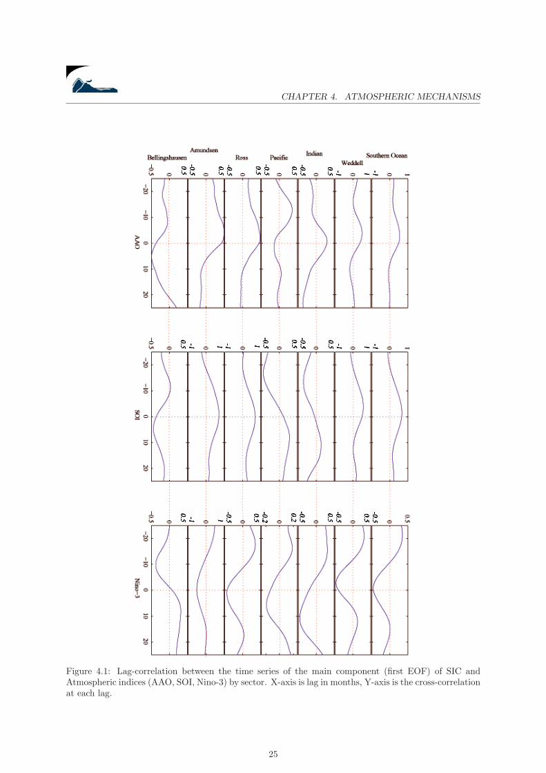
in figure 4.1 displaying the lag-correlation values of the three atmospheric indices with SIC depending

on the lag l.

The largest correlation seems to be between SIC and SOI, which is fairly consistent with Yuan (2004)

who has shown that AAO and ENSO explain a significant part of Antarctic sea ice variability. At

zero-lag, the correlation between SIC and SOI are quite strong for the whole Southern Ocean, but also

regionally for the Weddell, Ross and Amundsen seas. The other areas present weaker lag-correlation

values (about 10 months for Pacific sector, 12 months for indian and Bellingshausen seas).

The Lag-correlation values with Nino-3 have weaker amplitudes but seem to be exactly out of phase

with the previous one (correlations have opposite signs). This was somewhat expected since SOI and

Nino-3 are indeed supposed to be out of phase by nature of the ENSO phenomenon.

Lag-correlation with AAO is quite alike the one with SOI in the whole Southern Ocean, Weddell and

Bellingshausen seas. Especially, the lags are quite consitent relatively to those observed for correlation

of SIC with SOI and Nino-3 (-10 months in Bellingshausen sea,-2 months in Weddell sea) which might

infer teleconnections between SAM and ENSO through sea ice (but this has never been truly studied

and is absolutely not an established fact).

What would eventually be interesting is to look closer at the lags between SIC and the atmospheric

indices in the vicinity of the Antarctic Dipole to find out insights on its variability. However this kind of

investigation has already been well conducted, Yuan and Martinson (2001), and considering the time we

had for this research project we preferred to focus on its Model/Observations comparison aspect since we

would not have time enough to push the study as far as the current state of the art. Nonetheless, these

calculations were very useful to verify that our EOF analyses and correlation computations give consistent

results and to ensure that we could apply them in the following without worrying about numerical our

mathematical issues. Indeed the direct study of SIC teleconnections with oceanic mechanisms would

have been much more difficult to validate since they have not truly been studied so far.

24

CHAPTER 4. ATMOSPHERIC MECHANISMS

Figure 4.1: Lag-correlation between the time series of the main component (first EOF) of SIC andAtmospheric indices (AAO, SOI, Nino-3) by sector. X-axis is lag in months, Y-axis is the cross-correlationat each lag.

25

Chapter 5

Oceanic mechanisms

5.1 Trends over the 15 years

Here we use outputs from the ECCO-GODAE model again, namely the three following 2D-fields: Sea

Surface Temperature (SST), Sea Surface Salinity (SSS) and Mixed-Layer Depth (MLD). We have the

time series of these fields also from 1992 to 2006.

Before looking at the correlation between these oceanic quantities and SIC we are interested in

analysing these fields by themselves, that is to say looking at their mean, trends and main EOF patterns.

To compute the trends, a linear regression was applied to each grid point of the three fields, so that:

oceanic field(i, j) = a(i, j) + b(i, j)× t

where t is the time in months. Thus the operation results in one ”a coefficient” and one ”b coefficient”

map for each kind of field. The following pictures display (fig. 5.1) the trend maps (patterns at zero-time

(a coefficient) and trend patterns over the 15 years (b coefficient)) of SST, SSS and MLD.

The ”a coefficient maps” give us an insight of the fields temporal mean (but it is not the real time-

mean itself). They are interesting especially for Mixed-Layer Depth (MLD) fields (fig. 5.1.c) because

they provide us with the evidence that the artifact in the Weddell sea is indeed an artifact, insofar as

negative values of MLD appear in the area (which is impossible). For Sea Surface Temperature (SST, fig.

5.1.a) we see that Ross, Amundsen and Bellingshausen regions seem to be hotter than Indian and Pacific

ones. As for Sea Surface Salinity (SSS, fig. 5.1.b), one can observe a circularly shaped pattern with weak

values of salinity close to the coasts and the antarctic continent. The trends map are also interesting,

26

CHAPTER 5. OCEANIC MECHANISMS

for both SSS and MLD fields they display quite uniform maps except at the location of the Weddell sea

artifact where trends are different from anywhere else (positive trend while trends are negative in the

rest of the southern ocean for exemple). On the SST trend map, we can also see a region with stronger

positive trend values between the Pacific sector and the Ross sea. Normally the EOFs computed further

should also corobarate these trends.

27


120

o W

60o W 0 o

60

o E

120o E

180 oW

84 o

S 72 o

S 60 o

S 48 o

S 36 o

S −2

0

2

4

6

8

10

120

o W

60o W 0 o

60

o E

120o E

180 oW

84 o

S 72 o

S 60 o

S 48 o

S 36 o

S

−6

−4

−2

0

2

4

6

x 10−3

(a) SST trend maps

120

o W

60o W 0 o

60

o E

120o E

180 oW

84 o

S 72 o

S 60 o

S 48 o

S 36 o

S 32.5

33

33.5

34

34.5

35

120

o W

60o W 0 o

60

o E

120o E

180 oW

84 o

S 72 o

S 60 o

S 48 o

S 36 o

S −4

−3

−2

−1

0

1

2

3

4x 10

−3

(b) SSS trend maps

120

o W

60o W 0 o

60

o E

120o E

180 oW

84 o

S 72 o

S 60 o

S 48 o

S 36 o

S −200

−100

0

100

200

300

400

500

600

120

o W

60o W 0 o

60

o E

120o E

180 oW

84 o

S 72 o

S 60 o

S 48 o

S 36 o

S −4

−3

−2

−1

0

1

2

3

4

(c) MLD trend maps

Figure 5.1: Trend maps of the three oceanic fields: SST, SSS and MLD. ”a coefficient” maps on the left,”b coefficient” maps on the right.

28


5.2 EOF Analyses

5.2.1 Sea Surface Temperature

In order to study the correlation of these oceanic fields with SIC, an EOF analysis was performed on

them so that we can apply the correlation analysis between the time series associated with the different

modes. The EOF analysis applied to SST gives curious results at first look. In terms of trend, it is

completely consistent with the previous maps. On the first mode (fig. 5.2.a), the ”positive anomaly”

area between Ross and Pacific sectors combined with an over-all upward tendancy of the associated time

series is consistent with what figure 5.1.a suggested. However SST and sea ice are tightly linked; and

to produce sea ice, temperature must decrease below the freezing point so the cooler the water is the

more chances there are to have sea ice. Thus one would have expected to find EOFs quite alike SIC ones

with an opposite sign (it is also what Yuan and Martinson (2001) suggest when defining the Antarctic

Dipole), but it is not the case. More precisly, considering the first EOF of model SIC data, the spatial

pattern presented the Antarctic Dipole shifted relatively to its real location. Then we would expect to

find the opposite dipole in the first spatial pattern of SST but instead we find this kind of pattern only

on the second EOF (fig. 5.2.b). Even so, we will see further that the correlation between the time series

associated with the first EOFs of SIC and SST is quite strong.

To explain this, we have to look closer and see that the variance of the second EOF of SST explains

for 20.03% of the total variance, which is almost as large as percentage of explained variance by the first

EOF (29.91%). So finally we do find a dipole-like pattern consistent with EOF analysis of SIC, but in

mode 2, and it does not prevent the first modes (of SIC and SSS) to be highly correlated. Indeed during

winter when SIC reaches its maximum, SIC and SST are strongly linked (spatially and temporally), but

during summer when there is no longer sea ice then the spatial correlation between both fields collapses.

That is why we observe a strong temporal correlation (inferred by the EOF time series) but different

spatial patterns.

29


120

o W

60o W 0 o

60

o E

120o E

180 oW

84 o

S 72 o

S 60 o

S 48 o

S 36 o

S

−0.03

−0.02

−0.01

0

0.01

0.02

0.03

0 20 40 60 80 100 120 140 160 180−30

−20

−10

0

10

20

30

(a) EOF1sst, explaining 29.91% of the total variance of the signal

120

o W

60o W 0 o

60

o E

120o E

180 oW

84 o

S 72 o

S 60 o

S 48 o

S 36 o

S

−0.03

−0.02

−0.01

0

0.01

0.02

0.03

0 20 40 60 80 100 120 140 160 180−25

−20

−15

−10

−5

0

5

10

15

20

(b) EOF2sst, explaining 20.03% of the total variance of the signal

Figure 5.2: EOF components of SST (left figures) with the associated time series (right figures) and theirfraction of explained variance.

30


5.2.2 Sea Surface Salinity

The positive trend of the first SSS EOF component (EOF1sss, Fig. 5.3a), and the positive anomaly in

the Weddell Sea are consistent with the trend maps (Fig. 5.1c). The problem is that this area is located

where the artifact is in the MLD fields, and it is not obvious determining whether it is due to it or not.

In fact one could have made the same comment for SIC first component (from model data), the negative

anomaly area in the Antarctic Dipole is the one where the signal is the strongest and also where the

MLD artifact seems to show up. As a consequence it seems likely that these signals are related or a

consequence of the MLD artifact.

At least what can be noticed is that for SIC and SSS these strong signals appear only on the first

EOFs whereas the artifact is clearly present on every MLD components (see next paragraph). Thus,

if there is indeed an artifact in the data due to a problem in the model, one is likely to find its origin

looking a bit closer at MLD data.

31


120

o W

60o W 0 o

60

o E

120o E

180 oW

84 o

S 72 o

S 60 o

S 48 o

S 36 o

S

−0.04

−0.03

−0.02

−0.01

0

0.01

0.02

0.03

0.04

0 20 40 60 80 100 120 140 160 180−15

−10

−5

0

5

10

(a) EOF1sss, explaining 30.81% of the total variance of the signal

120

o W

60o W 0 o

60

o E

120o E

180 oW

84 o

S 72 o

S 60 o

S 48 o

S 36 o

S

−0.05

−0.04

−0.03

−0.02

−0.01

0

0.01

0.02

0.03

0.04

0.05

0 20 40 60 80 100 120 140 160 180−15

−10

−5

0

5

10

(b) EOF2sss, explaining 18.50% of the total variance of the signal

Figure 5.3: EOF components of SSS (left figures) with the associated time series (right figures) and theirfraction of explained variance.

32


5.2.3 Mixed-Layer Depth

Like it was mentioned in the previous part, the dominant signal in all MLD components is the artifact-

looking one in the Weddell sea (fig. 5.3) . That could mean MLD estimate from the model is tightly

linked with the origin of the problem and it would not be surprising. Indeed MLD combined with SST

gives us a good idea of the heat content under the ice, and sea ice forms and melts depending on this

heat content. Considering EOF1sst and EOF1mld (fig. 5.3.a) conjointly, one can see a positive SST

anomaly in the Weddell sea associated with big values of MLD (artifact), which implies a great heat

content under the ice in this area. That could consequently cause a melting of the ice and also the SIC

strong negative anomaly in the Weddell part of EOF1mod (fig. 3.1.a). The issue becomes to know why

the MLD in this area is abnormally big.

120

o W

60o W 0 o

60

o E

120o E

180 oW

84 o

S 72 o

S 60 o

S 48 o

S 36 o

S

−0.03

−0.02

−0.01

0

0.01

0.02

0.03

0 20 40 60 80 100 120 140 160 180−1.5

−1

−0.5

0

0.5

1

1.5x 10

4

(a) EOF1mld, explaining 38.39% of the total variance of the signal

120

o W

60o W 0 o

60

o E

120o E

180 oW

84 o

S 72 o

S 60 o

S 48 o

S 36 o

S

−0.03

−0.02

−0.01

0

0.01

0.02

0.03

0 20 40 60 80 100 120 140 160 180−1

−0.5

0

0.5

1

1.5x 10

4

(b) EOF2mld, explaining 17.02% of the total variance of the signal

Figure 5.4: EOF components of MLD (left figures) with the associated time series (right figures) andtheir fraction of explained variance.

33


5.3 Correlation Analyses

Thanks to the EOF analysis already performed we have the time series associated with the components

of the SIC, SST, SSS and MLD fields. The next figure (5.5) shows the lag-correlation plots between these

expansion coefficients. It would have probably been more rigorous to perform an SVD decomposition

analysis between SIC and the other fields, but this simple lag-correlation analysis provide us with a fairly

good insight of how these physical parameters are related.

The first remark one can do is about the general strong zero-lag correlation between SIC in the

whole Southern Ocean and SST. On the contrary one could have expected an anticorrelation since the

colder the water is the more ice it is likely to be formed, but since the EOF patterns already have

opposite signs (see EOF1obs and EOF1sst) it is consistent. If one consider the regional correlations, the

Amundsen, Ross and Weddell sectors present a strong correlation between SIC and SST (at zero-lag).

The other areas display non-significant lag-correlations except Bellingshausen sea where the 10-months

lag anticorrelation is about -0.5.

For the correlation values with SSS and MLD, they are almost all equal to zero, which does not

give us a lot of information. The lag-correlation are not really significant either. There is a positive

10-months lag-correlation between SIC and SSS in Bellingshausen Sea that we might be tempted to

relate with the lag-correlation in SST. Indeed as the correlations have opposite signs we could associate

this to a density-conservation phenomenon, if there is a increase (resp. decrease) in the SST anomaly

then a decrease (resp. increase) in SSS anomaly would occur to compensate the the SST change and

maintain density. However the latter lag-correlation value is very weak (less than 0.2) and what is more

if one consider for example Pacific sector, there the two lag-correlations have the same sign, and the

explanation is no longer plausible.

Also in the Weddell plot of lag-correlation between SIC and MLD, the negative correlation at zero-lag

is something one could have expected. With respect to the fact that the MLD artifact is located in the

Weddell Sea, we could expect a strong anticorrelation in the vicinity of the area, insofar as a sharp

increase in MLD anomaly should induce a melting of the ice (and MLD time series variations are indeed

quite sharp, see figure 3.4). Even so the anticorrelation value is not that important. This has to be linked

with the first remark of this section, a lag-correlation calculation between the time series coming from a

true SVD analysis of coupled fields may have given more significant results (it was not done because of

a lack of time but it would be an interesting investigation to perform for a further study). Last but not

least, the outputs of the model are likely to be affected by the model issues quite differently depending on

34


their nature and the considered area. That could consequently make the correlation results non-uniform.

Figure 5.5: Lag-correlation between the time series of the main components (first EOF) of SIC andOceanic fields (SST, SSS, MLD) by sector. X-axis is lag in months, Y-axis is the cross-correlation ateach lag.

35

Chapter 6

Conclusions

At the beginning of the study, the goal of the project was two-folded. The first aspect was to study

satellite observations of sea ice concentration to complete existing works about Southern Ocean sea ice

variability and the second was to compare the ECCO-GODAE v.3 sea ice state estimate with these

observations in order to assess its quality. As it was mentionned in the introduction, several groups have

studied the teleconections between sea ice variability and atmospheric phenomena like El Nino/Southern

Ocean or the Antarctic Oscillation (AAO) very well, but nobody really studied the potential linkages

with oceanic phenomena. Thus the first step was to look at the SIC variability in itself to coroborate

what had been done before on the present field and in the same way to check that our different methods

of data analysis were giving suitable results (like for EOF analysis for example). Then knowing our

routines worked properly we could apply them to the outputs of the model (SIC estimate, SST, SSS,

MLD) and intend to find correlations between the results. Mainly due to time constraints, we were not

able to carry out these two works completely. However some relevant indications on the model estimates

were established.

With respect to the Antarctic sea ice variability characterization, the study did not go further than

the conclusions plublished by other groups like Parkinson (2004) who achieved the same kind of analysis

based on both observations and data provided by models. Once the seasonal cycle is removed from the

SIC or sea ice integrated area signals, the residuals exhibits a positive trend of 1400 km2month−1 for the

observations and -4000 km2month−1 for the ECCO estimate, an inconsistancy that remains unexplained,

but may be also linked with the MLD articfact. The EOF and SVD analyses performed on SIC fields

enabled to confirm the existence of the Antarctic Dipole (ADP) through the correlation calculations

between time series of Bellingshausen-Weddell and Ross-Amundsen seas. This ”wavenumber-2 mode”

36

CHAPTER 6. CONCLUSIONS

was also naturally found in the second EOF of SST (although we would primarily have expected to find

it on the first EOF pattern). The ice variablity, somehow represented by the time series associated with

the first of its EOF components, presents some strong correlations with the Southern Annular Mode

(SAM) and ENSO-related indices (0.6 with AAO and SOI, -0.5 with Nino-3 at zero-lag for the whole

Southern Ocean) which is consistent with previous work (e.g. Yuan (2004)). The overall correlation, or

rather the overall anticorrelation between SIC and SST at zero-lag are as strong as expected although

they weaken in some regions like Indian, Pacific or Bellingshausen seas. One must keep in mind that SIC

and SST have a different nature in the correlation study (one is observations while the other was derived

from the model), so this is probably resulting from some issues with the sea ice estimate in the model.

The amplitude of the cross-correlation of SIC and SSS or MLD are less significant. These oceanic fields

estimated by the model were also very useful to corroborate and exhibits some defects first observed in

the ECCO-GODAE SIC estimate. It seems that the model always underestimates the observations ice

integrated area. Furthermore the standard deviation maps of the misfit between observations and model

show that it also undervalues the Ice Extent (Sea Ice Edge). These maps also exhibits strong values of

the misfit in the vicinity of Weddell sea where an articfact from model data were identified afterwards.

Indeed, it was noticed that strong anomalies in Mixed-Layer Depth (especially in the Weddell sea) could

generate the artifacts observed on the other fields derived from the model. To figure out what the root of

the problem is, one should know much better how the model works to understand why the mixed-layer

depth sharply deepens in these areas, thus drasticly changing the heat content under the ice and causing

it to melt abnormaly. However, this is currently far from being within the range of our study and would

require much more time than we had. The research obviously needs to be continued, and for further

analysis, one should go into details between sea variability and oceanic processes. Subsequently the first

step would likely be understanding the model code and why it creates the MLD issue. Once the problem

is solved, the correlation calculations would have to be reprocessed with true SVD of coupled fields

analysis in order to establish sufficiently reliable lag-correlation plots. The most interesting part of the

work would then be to come back to the ice variability aspects by combining the resulting curves. Looking

at the cross-correlation values depending on both lags and regions of Antarctic, one may hopefully be

able to identify dynamical processes propagating from one sector to another (through the annular mode

or different kinds of waves) and potentially explaining a substantial part of the southern ocean sea ice

variability.

37

Appendix A

EOF/PCA and SVD analysis of

Climatic Data

Except some comments and some changes in the problem’s formalism, the main part of the following

was taken from ”A Manual for EOF and SVD analyses of Climatic Data”, by H. Bjornsson and S. A.

Venegas. Some sections are also refering to ”Statistical Analysis in Climate Research”, by Hans von

Storch and Franci W. Zwiers.

A.1 What is it all about and when to use each method

This appendix contains a fairly dicussion of two methods for analysing the spatial and temporal variability

of geophysical fields. The two methods covered are the method Empirical Orthogonal Functions (EOFs),

also known as Principal Component Analysis (PCA), and the method of Singular Value Decomposition

(SVD). The EOF/PCA analysis is a method of choice for analysing the variability of a single field, i.e. a

field of only one scalar variable (SLP, SST etc). The purpose is to find the spatial patterns of variability,

their time variation, and gives a measure of the ”importance” of each pattern. As the method is tightly

linked with eigenvalues and eigenvectors calculations, the SVD analysis can be used for both single fields

EOFs determination and coupled fields analyses. The SVD applied to two fields together will identify

the modes modes of behavior in which the variations of the to fields are strongly coupled. It should be

stressed that even though the methods presented below break the data into ”modes of variability”, these

modes are primarily data modes, and not necessarily physical modes. Whether they are physical will be

matter of subjective interpretation. One more remark about terminology before we get started, the EOF

38

APPENDIX A. EOF/PCA AND SVD ANALYSIS OF CLIMATIC DATA

method finds both time series and spatial patterns. Most authors refer to the patterns as the ”EOFs”,

but some refer to them as the ”Principal component loading patterns” or just ”principal components”.

The time series are referred to as ”EOF time series”, ”expansion coefficient time series”, ”expansion

coefficients”, ”principal component time series” or just ”principal components”. In what is described

herein, we will refer to the patterns as the EOFs and the time series as ”principal components (PCs)”

or ”expansion coefficients”.

A.2 The Data

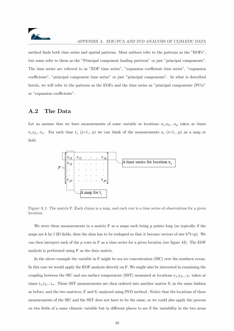
Let us assume that we have measurements of some variable at locations x1,x2,...xp taken at times

t1,t2,...tn. For each time tj (j=1,...n) we can think of the measurements xi (i=1,...p) as a map or

field.

Figure A.1: The matrix F. Each clumn is a map, and each row is a time series of observations for a givenlocation.

We store these measurements in a matrix F as n maps each being p points long (so typically if the

maps are k by l 2D fields, then the data has to be reshaped so that it become vectors of size k*l=p). We

can then interpret each of the p rows in F as a time series for a given location (see figure 43). The EOF

analysis is performed using F as the data matrix.

In the above example the variable in F might be sea ice concentration (SIC) over the southern ocean.

In this case we would apply the EOF analysis directly on F. We might also be interested in examining the

coupling between the SIC and sea surface temperature (SST) measured at locations y1,y2,...yr taken at

times t1,t2,...tn. These SST measurements are then ordered into another matrix S, in the same fashion

as before, and the two matrices, F and S, analysed using SVD method. Notice that the locations of these

measurements of the SIC and the SST does not have to be the same, so we could also apply the process

on two fields of a same climatic variable but in different places to see if the variability in the two areas

39


are close or not (this is what we use while looking at the SIC covariability between the different sectors

of southern ocean for example).

A.3 How to do it

A.3.1 Principle

Let us assume that we removed the mean from each of the p time series in F, so that every row has zero

mean.1

We form the covariance matrix of F by calculating R= 1N−1FtF and then we solve the eigenvalue

problem

RC = CΛ. (A.1)

Λ is a diagonal matrix containing the eigenvalues λi of R. The ci column vectors of C are the

eigenvectors of R corresponding to the eigenvalues λi. Both Λ and C are of the size pn bby n. Each of

these eigenvectors can the be regarded as a map, and they are the EOFs we were looking for. In what

follows we always assume that the eigenvectors are ordered according to the size of the eigenvalues (EOF1

is the eigenvector associated with the biggest eigenvalue, and the one associated with the second biggest

eigenvalue is EOF2, etc). Each eigenvalue λi, gives a measure of the fraction of the total variance in R

explained by the mode. This fraction is found by dividing the λi by the sum of all the other eigenvalues

(the trace of Λ).

The eigenvector matrix C has the property that CtC=CCt=I (where I is the identity matrix). This

means the EOFs are uncorrelated over space. Another way of stating this is to say that the eigenvectors

are orthogonal to each other. Hence the name Empirical Orthogonal Functions (EOF).

The pattern abtained when an EOF is plotted as a map, represents a standing oscillation. The time

evolution of en EOF shows how this pattern oscillates in time. To see how EOF1 ’evolves’ in time we

calculate:

~a1 = F ~c1 (A.2)

The n components of the vector ~a1 are the projections of the maps in F on EOF1, and the vector is a

time series for the evolution of EOF1. In general, for each calculated EOFj, we can find a corresponding

~aj . These are the principal component time series (PC’s) or the expansion coefficients of the EOFs. Just

1Removing the time means has nothing to do with the process of finding eigenvectors, but it allows us to interpret Ras the covariance matrix, and hence understand the results. Strictly speaking you can find EOFs without removing anymean, or you can remove the mean of each map, but not each time series.

40


as the EOFs were uncorrelated in space, the expansion coefficients are uncorrelated in time.

We can reconstruct the data from the EOFs and the expansion coefficients:

F =p∑

j=1

~aj(EOFj) (A.3)

A common use of EOFs is to reconstruct a ’cleaner’ version of the data by truncating this sum at some

j = N ¿ p, that is, we only use the EOFs of the few largest eigenvalues. The rationale is that the first

N eigenvectors are capturing the dynamical behavior of th system, and the other eigenvectors of the

smallest eigenvalues are just due to random noise. Needless to say this assumption is not always true.

A.3.2 How to compute it

The remaining issue is: How to solve the eigenvector and eigenvalue problem? One approach is to use

Singular Value Decomposition (SVD). Indeed any m×n matrix A can be given a SVD:

A = USV †

where U is m×n, S is n×n, V is n×n, and V† is the conjugate transpose of V (U and V are orthogonal

matrices). The first min(m,n) columns of U and V are orthgonal vectors of dimension n and m and

are called left and right singular vectors, respectively. Matrix S is a diagonal matrix with non-negative

elements sii=si, i=1,...,min(m,n), called singular values. All other elements of S are zero. Therefore:

AA†U = USV †V SU†U = US2

A†AV = V SU†USV †V = V S2

That is, the columns of V are the eigenvectors of A†A, the squares of the singular values si are the

eigenvalues of A†A, and the columns of U are the eigenvectors of AA† that correspond to these eigenvalues.

Note that all this is true when m≥n, when m<n we first write the SVD of A† = U ′S′V ′† where U’ is

n×m, S’ is m×m, and V’ is m×m, all with the properties as described above. Thus A=V’S’U’†.

Let us mention also a theorem that is often useful when computing eigenvalues and eigenvectors:

Theorem 1 Let A be any m×n matrix. If λ is a nonzero eigenvalue of multiplicity s of A†A with s

linearly independent eigenvectors ~e1, ..., ~es, then λ is also an s-fold eigenvalue of AA† with s linearly

independent eigenvectors A~e1, ..., A~es.

41


So, let us take again the data matrix F. In order to remove the temporal mean from the data (i.e.

we consider the anomaly field) we compute the matrix:

χ = F (I − 1n

J)

where I is the n×n identity matrix and J is the n×n matrix composed entirely of units. Therefore the

covariance matrix is:

Σ =1n

χχ†

As a consequence, If the sample size n is larger than the dimension of the problem p, then the EOFs are

calculated directly as the normalized eigenvectors of the p×p matrix Σ. On the other hand, if the sample

size, n, is smaller than the dimension of the problem, p, the EOFs may be obtained by first calculating

the normalized eigenvectors ~g of the n×n matrix Σ = 1n (I − 1

nJ)F †F (I − 1nJ), and then according to

the previous theorem, computing the EOFs as

~e =F (I − 1

nJ)~g‖F (I − 1

nJ)~g‖ .

Now the SVD of the p×n centred data matrix

χ = F (I − 1n

J),

is

χ = USV †

and therefore1n

χ†χV =1n

V S2.

So the eigenvectors of Σ are the columns of V and the corresponding eigenvalues are 1nS2. One can

finally retrieve the EOFs from these eigenvectors thanks to theorem 1 and the expansion coefficients by

calculating ~aj = F × EOFj since they are nothing but the projection of F onto the j-th EOF. It is also

interesting to compute the variance ratio of each EOF from the eigenvalues λi = 1ns2

i by computing

λi∑λi

.

This last quantity provide us with the ’amount of variance explained’ by each EOF.

42


A.3.3 How to understand it physically

Let us take a physical (and unrealistic) example. We have Pacific SST data, one SST map per month

sampled over a period of a few decades, that we put in a data matrix without removing the temporal

mean. We perform an EOF analysis and find that most of the data is explained by 2 eigenvectors only.

The first one (EOF1) is a map of contours that are positive in the northern hemisphere and negative

in the southern hemisphere. The corresponding PC is periodic with a period of about 12 months. We

therefore identify EOF1 as the annual cycle. EOF2 shows many contour lines close to the equator but

few elsewhere and the associated PC is quasi-periodic with a period of few years. We identify this

eigenvector to be associated with El Nino. From this data we would get the picture of Pacific SSTs and

their evolution in time: most of what happens is described by the SST change associated with the annual

cycle and the slower SSt change associated with El Nino. And since no other eigenvectors contribute

much (all other eigenvalues are very small) we assume that everything else found in the observations is

just noise. The EOF method thus allows us to view all the complicated variability in the original SST

data and explain it by two processes.

In practice it is inadvisable to keep the seasonal cycle in the data, since that signal is likely to

dominate everything else. That is why we often begin the analysis by removing the seasonal cycle from

the data using an appropriate filtering method.

A.3.4 SVD of coupled fields

The singular Value Decomposition (SVD) method can be thought of as a generalization to rectangular

matrices of the diagonalization of a square symmetric matrix (like in EOF anlysis). I is usally applied

in geophysics to two combined data fields, such as SLP and SST. The method identifies pairs of coupled

spatial patterns, with each pair explaining a fraction of the covariance between the txo fields. Hence, to

perform this decomposition, we construct the temporal cross-covariance matrix between two space and

time dependent data fields. As an example, let us assume we have two data matrices, S and I (S being

SST fields and I Ice concentration fields). Let us suppose that S is p×n and I is q×n (that means S and

I have been reshaped like F in the previous parts, so that their rows contain a time series for a particular

location, and their columns contain a map for a given time). Then if both S and I are centred in time,

then the cross-covariance matrix is C = S†P . This matrix does not need to be square as the two fields

may be defined on a different number of grid points.

The SVD

C = ULV †

43


of the cross-covariance matrix yields two spatially orthogonal sets of singular vectors (spatial patterns

analogous to the eigenvectors or EOFs, but one for each variable) and a set of singular values associated

with each pair of vectors (analogous to the eigenvalues). The singular vectors for S are the columns of

U, and the singular vectors for P are the columns of V. Each pair of spatial patterns describe a fraction

of the square covariance (SC) between the two variables (i.e. is a mode of co-variability between the

two fields). The first pair of patterns describes the largest fraction ot the SC and each succeeding pair

describes a maximum fraction of SC that is unexplained by the previous pairs. Just as with the EOFs,

these patterns represent standing oscillations in the data fields and we can find the expansion coefficients,

i.e. time series describing how each mode of variability oscillates in time. For S and P we respectively

calculate A = SU and B = PV (the k-th expension coefficient for each variable is computed by projecting

the corresponding original data field onto the k-th singular vector). The columns of the matrices A and

B contain the expension corfficients of each mode. The diagonal of L contains the singular values and

the total squared covariance in C is given by the sum of the squared diagonal values of L. This gives a

simple way of assessing the relative importance of the singular modes, through the squared covariance

fraction (SCF) explained by each mode. If li=L(i,i) is the i-th singular value, the fraction of squared

covariance explained by the corresponding singular vectors ~ui and ~vi is given by

SCFi =li

trace(L).

Finally the correlation value (r) between the k-th expansion coefficients ot the two variables indicates

how strongly related the k-th coupled patterns are.

44

Appendix B

Dates of Minimum and Maximum

SIC

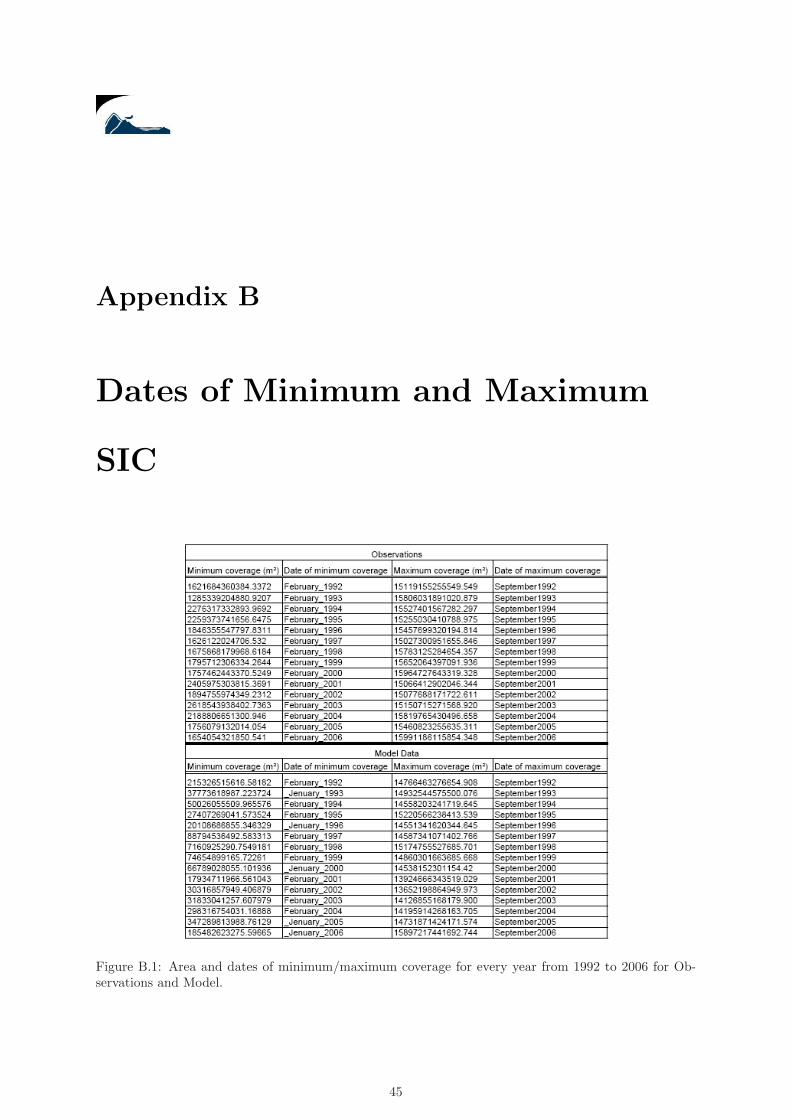
Figure B.1: Area and dates of minimum/maximum coverage for every year from 1992 to 2006 for Ob-servations and Model.

45

Appendix C

AAO, SOI and Nino-3 Indices

∗The Antarctic Oscillation (AAO) is the dominant pattern of non-seasonal tropospheric circulation

variations south of 20S, and it is characterized by pressure anomalies of one sign centered in the Antarctic

and anomalies of the opposite sign centered about 40-50S. The AAO is also referred to as the Southern

Annular Mode (SAM). The daily AAO index is constructed by projecting the daily 700mb geopotential

height anomalies poleward of 20S onto the loading pattern of the AAO, the loading pattern of the AAO

being defined as the leading mode of Empirical Orthogonal Function (EOF) analysis of monthly mean

700 hPa height during 1979-2000 period (see fig. C.1).

∗The Southern Oscillation Index (SOI) is one measure of the large-scale fluctuations in air pressure

occurring between the western and eastern tropical Pacific (i.e., the state of the Southern Oscillation)

during El Nio and La Nia episodes. It is computed using monthly mean sea level pressure anomalies at

Tahiti (T) and Darwin (D). The SOI [T-D] is an optimal index that combines the Southern Oscillation

into one series.

∗El Nio-Southern Oscillation (ENSO; commonly referred to as simply El Nio) is a global coupled

ocean-atmosphere phenomenon. The Pacific ocean signatures, El Nio and La Nia are important tem-

perature fluctuations in surface waters of the tropical Eastern Pacific Ocean. NINO3 is an index that

measures the strength of an ENSO event: it is the SST anomaly averaged over [5S,5N] and [150W,90W],

i.e. the eastern equatorial Pacific. The atmospheric signature of ENSO is the Southern Oscillation (SO).

46

APPENDIX C. AAO, SOI AND NINO-3 INDICES

Figure C.1: Taken from NOAA Climate Prediction Center Website.

47

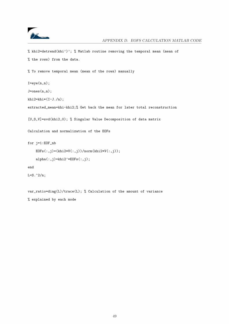
Appendix D

EOFs calculation MATLAB code

During my research work, I had to implement a huge number of codes to obtain the results presented in

this report. To avoid overloading the report and for the sake of paper saving I just put the EOF statistical

tool Matlab code in appendix.

function [alpha, EOFs,var_ratio,extracted_mean]=EOF(k,n,data,EOF_nb)

%-------------------------------------------------------------------------%

% alpha = Time-series associated with the EOFs

% EOFs = Components resulting from Singular Value Decomposition after

% re-normalization

% var_ratio = amount of variance explained by each EOF

% extracted_mean = Temporal mean of the data, necessary for field

% reconstruction from EOFs

%-------------------------------------------------------------------------%

% data = Input data

% n = Number of samples

% k = Dimension of the problem, number of positions of the problem

% EOF_nb = Number of EOFs wanted in output

%-------------------------------------------------------------------------%

khi=reshape(data,k,n); % Data formating

khi(find(isnan(khi)))=0;

48

APPENDIX D. EOFS CALCULATION MATLAB CODE

% khi2=detrend(khi’)’; % Matlab routine removing the temporal mean (mean of

% the rows) from the data.

% To remove temporal mean (mean of the rows) manually

I=eye(n,n);

J=ones(n,n);

khi2=khi*(I-J./n);

extracted_mean=khi-khi2;% Get back the mean for later total reconstruction

[U,S,V]=svd(khi2,0); % Singular Value Decomposition of data matrix

Calculation and normalization of the EOFs

for j=1:EOF_nb

EOFs(:,j)=(khi2*V(:,j))/norm(khi2*V(:,j));

alpha(:,j)=khi2’*EOFs(:,j);

end

L=S.^2/n;

var_ratio=diag(L)/trace(L); % Calculation of the amount of variance

% explained by each mode

49

Bibliography

Carleton, A., 2003: Atmospheric teleconnections involving the Southern Ocean. J. Geophys. Res,

108 (C4), 8080.

Cavalieri, D. J. and C. L. Parkinson, 2008: Antarctic sea ice variability and trends, 19792006. Journal

of Geophysical Research, 113, C07 004, doi:10.1029/2007JC004564.

Holland, M., C. Bitz, and E. Hunke, 2005: Mechanisms Forcing an Antarctic Dipole in Simulated Sea

Ice and Surface Ocean Conditions. Journal of Climate, 18 (12), 2052–2066.

Kwok, R. and J. Comiso, 2002: Southern Ocean Climate and Sea Ice Anomalies Associated with the

Southern Oscillation. Journal of Climate, 15 (5), 487–501.

Liu, J., J. Curry, and D. Martinson, 2004: Interpretation of recent Antarctic sea ice variability. Geophys.

Res. Lett, 31 (2), 1–4.

Parkinson, C., 2004: Southern Ocean sea ice and its wider linkages: insights revealed from models and

observations. Antarctic Science, 16 (04), 387–400.

Serreze, M., M. Holland, and J. Stroeve, 2007: Perspectives on the arctic’s shrinking sea-ice cover.

Science, 317, 1533–1536, doi:10.1126/science.1139426.

White, W. and R. Peterson, 1996: An Antarctic circumpolar wave in surface pressure, wind, temperature

and sea-ice extent. Nature, 380 (6576), 699–702.

Wunsch, C. and P. Heimbach, 2007: Practical global oceanic state estimation. Physica D, 230(1-2),

197–208.

Yuan, X., 2004: ENSO-related impacts on Antarctic sea ice: a synthesis of phenomenon and mechanisms.

Antarctic Science, 16 (04), 415–425.

50

BIBLIOGRAPHY

Yuan, X. and D. Martinson, 2000: Antarctic Sea Ice Extent Variability and Its Global Connectivity.

Journal of Climate, 13 (10), 1697–1717.

Yuan, X. and D. Martinson, 2001: The Antarctic dipole and its predictability. Geophys. Res. Lett,

28 (18), 3609–3612.

Zwally, H., J. Comiso, C. Parkinson, D. Cavalieri, and P. Gloersen, 2002: Variability of Antarctic sea ice

1979–1998. J. Geophys. Res, 107 (10.1029).

51

Date post:	27-Mar-2018
Category:	Documents
Upload:	nguyencong
View:	215 times
Download:	0 times

End of Training Project Report - UCLouvain of Training Project Report September10, 2008 Patterns and...

Documents