Endogenous Group Formation and its impact on

Cooperation and Surplus Allocation

- An Experimental Analysis

by

Sibilla Di Guida, The Anh Han, Georg Kirchsteiger,

Tom Lenaerts and Ioannis Zisis

Discussion Papers on Business and Economics

No. 8/2020

FURTHER INFORMATION

Department of Business and Economics

Faculty of Business and Social Sciences

University of Southern Denmark

Campusvej 55, DK-5230 Odense M

Denmark

ISSN 2596-8157 E-mail: Lho@sam.sdu.dk / http://www.sdu.dk/ivoe

1

Endogenous Group Formation and its impact on Cooperation and Surplus Allocation - An Experimental Analysis

Sibilla Di Guida, The Anh Han, Georg Kirchsteiger, Tom Lenaerts, and Ioannis Zisis

Sibilla Di Guida: Corresponding author, Department of Business and Economics, University of

Southern Denmark, Campusvej 55, 5230 Odense M, Denmark; Email: sidg@sam.sdu.dk, ORCID ID:

0000-0002-3548-4733

The Anh Han: School of Computing, Teesside University, Middlesbrough, Tees Valley, TS1 3BX, UK;

Email: T.Han@tees.ac.uk

Georg Kirchsteiger: ECARES, Université Libre de Bruxelles, Avenue Roosevelt 50, 114 Bruxelles,

Belgium, CEPR, CESifo, and VCEE; Tel: + 32 2 650 42 12 Email: gkirchst@ulb.ac.be

Tom Lenaerts: Vrije Universiteit Brussel, MLG, Université Libre de Bruxelles and Ai-lab, Boulevard

du Triomphe, 212 Bruxelles, Belgium; Email: tlenaert@ulb.ac.be

Ioannis Zisis: MLG, Université Libre de Bruxelles; Boulevard du Triomphe, 212 Bruxelles, Email:

izisis@ulb.ac.be

Declaration of interest: none

Acknowledgements and Funding sources

The authors thank Carlos Alos-Ferrer, and the other organizers of the Cologne Laboratory for

Economic Research.

The authors acknowledge the financial support of the "Fonds de la Recherche Fondamentale

Collective", grant nr. 2.4614.12, and of the "Fonds Wetenschappelijk Onderzoek - FWO", grant nr.

G.0391.13N. None of the funding sources were involved in designing the study, in the collection,

analysis, and interpretation of the data, in the writing of the report, in the decision to submit the

article for publication.

2

Abstract

This paper investigates how endogenous group formation combined with the possibility of repeated interaction impacts cooperation within groups and surplus distribution. We developed and tested experimentally a Surplus Allocation Game where cooperation of four agents is needed to produce surplus, but only two have the power to allocate it among the group members. Different matching procedures were used to test the impact of exogenous vs. endogenous group formation. Our results show that repeated interaction with the same partners (endogenous group formation) leads to a self-selection of agents into groups with different life-spans, whose duration is correlated with the behavior of both distributors and receivers. While behavior at the group level is diverse for surplus allocation and amount of cooperation, aggregate behavior is instead similar when groups are exogenously or endogenously formed. Our results cast doubts whether the possibility of repeated interaction can lead to cooperation and efficient outcomes when the ex-post bargaining power about the surplus distribution is very unequal. Rather, it seems to amplify differences in the cooperation and distribution behavior across groups.

JEL Classification: C72, C92, D03

Keywords: cooperation, surplus distribution, exogenous group formation, endogenous group

formation

PsycINFO Classification: 2340, 2360, 3020

3

1. Introduction

One defining aspect of human life is cooperation. Cooperation is at the core of the relations between

family members and friends, as cooperation between co-workers is crucial for any employment

relationship. While cooperation fulfils many needs of human beings, one main reason for the

paramount importance of cooperation is the production of surplus. A cooperating group can

achieve more than the sum of what each individual can achieve on his/her own. This holds true for

co-workers assembling a car as well as for the founders of a modern startup or scientists

collaborating on a research project.

Even though the production of surplus provides an incentive to cooperation, it also has the

potential to cause conflicts, which will lead to an efficiency loss. It is well known that subjects care

about allocative fairness and may even give up own payoff in order to prevent unfair outcomes (for

an overview of the experimental evidence see e.g. Cooper and Kagel 2016). In our context this

implies that if the distribution of the surplus is not satisfactory for all cooperating agents, some

agents might stop cooperating, and if an unsatisfactory surplus distribution is foreseen, cooperation

might be prevented from the very beginning. Successful cooperation requires a split of the surplus

that is satisfactory for all agents involved in the generation of the surplus (Fung and Au 2014).

Obviously, if enforceable contracts can be signed a-priori, the problem of a satisfactory surplus

distribution can be easily solved. But such contracts are often not feasible, e.g. because it might be

impossible to foresee all the contingencies that can occur during the surplus production. Without

binding a-priori contracts, the final surplus distribution is determined by the bargaining power the

agents have after the surplus is already produced. In case agents have very uneven bargaining

power, cooperation might be refused a-priori by those agents who expect to have low ex-post

bargaining power.

Repeated cooperation and information about past surplus distribution may appear to solve or

reduce the problem of uneven bargaining power, leading to efficient cooperation and satisfactory

surplus allocation. There are two reasons for that: On the one hand, repeated surplus distribution

might allow the weak agents to get information about the specific behavior of each individual

strong agent. Hence, the weak agents can cooperate or not depending on the past behavior of their

strong partners. This provides the strong agents with an incentive not to abuse their bargaining

power, leading to more cooperation and more equal surplus distribution (see e.g. Ellison 1994). If

information on prior behavior is provided, this mechanism holds when the group formation

changes exogenously. Take as an example a re-assignment of workers within the same firm; it is

4

likely that despite the re-assignment, workers have some information about the past behavior of

their new teammates, and that this influences their cooperation.

On the other hand, repeated interaction with the same partners provides an additional reason to

enhance cooperation and a more equal surplus allocation: The weak agent can directly threaten the

strong one to refuse cooperation in the future, forcing the strong one to accept a surplus

distribution that is satisfactory for all agents involved. Take for example a group of workers that get

a joint bonus if their joint production fulfils some criteria, then assume that one of the co-workers

(e.g. the foreman) has a decisive influence on the distribution of the bonus between himself and the

others. If the foreman would ensure himself the lion share of the bonus, his co-workers would

refrain from cooperating next time, and this threat forces the foreman to find a fair distribution

(whatever might be perceived as fair in the particular context).

The well-known folk theorem (see Fudenberg and Maskin 1986) is often interpreted as showing

that repeated interaction improves efficiency. A typical example is the relational contract literature

(see e.g. Baker et al. 2002). However, this analysis does not take into account that, in many contexts,

agents might not only refuse to cooperate with given partners (and get an exogenously determined

value of an outside option), but they might also switch partners altogether. Again, take the example

of the working group. Unfairly treated workers might decide to quit and change team or look for

another job, possibly making it harder for the remaining group members to fulfil the criteria for the

bonus.

In this paper we analyze experimentally how the possibility of affecting group composition impacts

the cooperation level of and the surplus distribution within groups. With this design, we capture all

those working situations where team members collaborate to a common goal, but where ex-post

bargaining power differs across members (such as in presence of seniority or hierarchy). As

information about past behavior is public, we can think about workers within a firm, which

collaborate to different projects. Once a new project is presented, workers can maintain the group

(team) structure if it has been successful previously or ask to be re-allocated to a different team.

The rest of the paper is organized as follows: In the next section (Section 2) we introduce the

literature that is more relevant for our research. Section 3 describes the experimental design. In

Section 4 we specify the hypotheses to be tested, while in section 5 we describe the experimental

results. The last section concludes.

5

2. Related literature

As the study of cooperation and the nature of groups (exogenously vs endogenously formed) are

relevant topics in many field of research, our results are linked with previous research developed in

fields very diverse in both focuses and goals.

In economics, the theoretical and experimental investigation of cooperation focuses mainly on

prisoner's dilemma games, starting with the classical study of Rapoport and Chamah (1965). As in

our paper, much of the existing analysis of prisoner's dilemma games focused on the impact of

repetition on cooperation (see e.g. Kreps et al. 1982 or Clark and Sefton 2001). However, in most of

this literature, repeated interaction is exogenously given (Camera and Casari 2009). Recently

attention has been devoted to the study of behavior in prisoner´s dilemma games where

partnerships can be endogenously terminated (Honhon and Hyndamn, unpublished results; Lee,

unpublished results). On this topic, the most relevant published article is Wilson and Wu (2017),

which focuses on the impact on cooperation of different costs of quitting an unsatisfactory

relationship.

As information on past behavior is available in our framework, our work touches also the field of

reputation. Previous results on reputation suggest that showing an “other regarding” behavior in

the past triggers trust and increases cooperation (Bohnet & Huck 2004, Bolton et al. 2005, Resnik et

al. 2006). In these experiments, matching is exogenous and subjects are allowed to choose the

preferred earnings allocation between fixed options, favoring either one or the other participant. It

remains therefore unanswered how group formation is affected by past behavior, and how such

group structure affects the perception of a fair allocation of earnings across subjects.

Our paper is also linked to the extensive literature on bargaining experiments, particularly

ultimatum and dictator game experiments (see e.g. Güth et al. 1982 and Forsythe et al. 1994; for an

overview of the experimental results of these games see Hoffman et al 2008). Results in the dictator

games show that subjects do not use all their bargaining power if this would lead to a very unequal

allocation. However, in these experiments, both surplus and matching are exogenously given.

Slonim and Garbarino (2007) show that allowing partner selection in a Trust and Modified Dictator

Game boosts trust and altruism. However, here partner selection is based on personal

characteristics (such as age and gender) and not past behavior. Hence, dictator game experiments

so far cannot answer the question of whether the endogenous possibility of repeated cooperation –

based on donations´ history – impacts cooperation level and the distribution of the surplus.

6

The ultimatum game is more similar to our surplus allocation game insofar, as in the ultimatum

game subjects with low bargaining power can refuse to cooperate. The experimental results show

that this possibility leads to more equal allocations than in the dictator games. But contrary to our

experiment, in ultimatum games the decision to cooperate is made by a receiver after he already

knows how the surplus is shared in case of cooperation. Hence, the ultimatum game models a

situation where binding a-priori contracts are feasible. Furthermore, in most ultimatum game

experiments, the matching is exogenous and therefore not connected to the cooperation decision.

Like dictator games, ultimatum game experiments cannot investigate how the endogenous

possibility of repeated cooperation impacts cooperation level and the distribution of the surplus.

A closer match to our paper is the research studying the yes/no games; i.e., ultimatum games where

respondents blindly decide whether to accept/reject a distribution (they are not told the

distribution before deciding, see Gehrig et al. 2007, Güth and Kirchkamp 2012). However, in this

literature, authors do not allow groups to build a common history based on repeated cooperation,

nor are interested in the effect played by past offers in group formation.

Finally, our paper is connected to the extensive experimental work on group formation. Group

formation is investigated mainly in the context of public good games (see Chaudhuri 2011 for a

review). Some papers investigate what happens to voluntary contributions to a public good when

groups are formed according to some exogenously given criteria (e.g. Gächter and Thöni 2005

where group members were exogenously matched according to their past contributions to a public

good). Experiments on endogenous group formation focus on particular aspects of group formation:

restricted vs free entry and exit (Ahn et al. 2008), costly entry (Coricelli et al. 2004), direct selection

from a pool of possible partners (Biele et al. 2008), group formed on the basis of stated preferences

(Page et al. 2005) or on previous donations to charitable organizations (Fehrler and Przepiorka

2016), the possibility of exclusion (Cinyabuguma et al. 2005, and Riedl and Ule 2002, unpublished

results), and mobility between groups (e.g. Ehrhart and Keser 1999). Recent research investigated

the impact of repeated cooperation in endogenously formed groups, however the settings

considered were rather different from ours, studying, among others, the use of punishment to

enhance cooperation (Fu et al. 2017), and the stability of cooperation in public projects with

stochastic outcomes, imperfect monitoring, and an exit option (Gaudeul et al. 2017).

In contrast to previous literature, our experiment studies a simple yet crucial mechanism whose

dynamics remain unclear: how the possibility to impact group composition affects the willingness

to cooperate and surplus allocation. Understanding how group dynamics unravel in such a

7

framework is crucial, as this context is easily encountered in many working situations involving

teamwork. To our knowledge, the only paper connecting partner choice with surplus distribution is

Debove et al. 2015. But unlike our paper, they focus on the impact of competition within stable

groups characterized by excess supply of either distributors or responders.

3. Experimental design

We developed a "Surplus Allocation Game" where groups consisting of two distributors and two

recipients were formed. Since we were interested in group behavior, we focused on groups of four

subjects equally split in distributors and recipients as this was the smallest symmetric group

possible (excluding pairs, which display a different behavior than groups; see e.g., Bornstein and

Yaniv, 1998). The experiment consisted of 30 rounds. At the beginning of the session, participants

were randomly assigned to the role of distributor or receiver. The role was maintained throughout

the experiment. In each round of the game, potential group members first had to decide individually

whether to cooperate with the proposed group or not; full acceptance was needed for surplus

production. The group surplus amounted to 20 ECUs per round. If at least one subject refused to

cooperate, no surplus was produced and all potential group members earned nothing that round.

Once the group was formed, the surplus produced had to be allocated among group members.

To model a situation with unequal ex-post bargaining power, each of the distributors received half

of the produced surplus (10 ECUs) that she (we stick to the convention that distributors are female

and receivers male) could then freely distribute between herself and the receivers. The

contributions of the two distributors were then summed up and divided equally between the two

receivers. A minimum contribution of 1 ECU was set, to avoid multiple equilibria in the game.

Before choosing whether to cooperate or not, all subjects were informed about how the matched

distributors allocated surplus in the last three rounds.1

Before the experiment started, participants were randomly allocated to cubicles, instructions were

read aloud by a lab assistant, and participants had to answer a control questionnaire to assure that

they understood the mechanisms of the experiment. Once everyone answered correctly all the

questions (explanations were repeated if necessary), the experiment started. After the experiment

1 No information was provided about the rounds in which matching has been refused and therefore distributors had not allocated surplus. A pilot study showed no effect of adding information of past refusal. Similarly, no difference has been observed when subjects received the average of the last three contributions, instead of the three single values.

8

was concluded, participants had to fill in a brief questionnaire, and then they were paid privately in

cash.

To test how the possibility to impact group composition affects cooperation and surplus

distribution, we designed three treatments: a baseline treatment, a re-matching treatment

(exogenous-matching), and an endogenous-matching treatment. In this setting, accepting the

proposed group coincides with the intention to cooperate, as subjects can only choose whether to

cooperate (accept the group) or not (refuse the group).

Baseline treatment (BT)

In the Baseline treatment (BT), we imposed cooperation on all four subjects. Groups were forcibly

formed and re-matched every round. Receivers were mere observers, while the two distributors

decided how to divide the surplus. Hence, BT was equivalent to a dictator game but with two

dictators (i.e. distributors) and two receivers forming a match.

This treatment was used as benchmark for the analysis of behavior in the next two treatments.

Re-match treatment (RT)

In the Re-match treatment (RT), cooperation was not enforced. Groups got exogenously re-matched

after each round, and in each round the four subjects decided whether to cooperate or not. If all

members decided to cooperate, the group proceeded as in the BT. If at least one of the members

decided not to cooperate, no surplus was produced and nobody on that proposed group earned

anything in that round. In order to build a history of contributions for the distributors, the RT

consisted of two phases. The first phase lasted three rounds and was identical to the BT -

cooperation was exogenously enforced, the surplus was distributed by the distributors, and the

subjects got re-matched every round. In the second phase (from round 4 to round 30) groups were

also randomly re-matched every round, but cooperation was not enforced anymore. All subjects

were informed about the three previous contributions of the distributors they were matched with;

with this information, each group member (both distributors and receivers) decided whether to

cooperate or not.

Comparing results from the BT and the RT allowed us to study how the possibility of refusing to

cooperate affected surplus allocation.

Endogenous-match treatment (ET)

The Endogenous-match treatment (ET) was similar to the RT, but for the fact that subjects would

maintain the same group composition, as long as all members agreed on cooperating. When at least

9

one member refused to cooperate, the group was dismantled. As the RT, also the ET was composed

of two phases. For the first three rounds (phase 1), groups were maintained, cooperation was

exogenously enforced, and the distributors made unilateral decisions about their contributions.

This phase was designed to build a past history of contributions. At the beginning of round 4 (phase

2), groups were randomly re-matched and information about past behavior was provided. From

round 4 onwards, subjects decided about cooperation. More specifically, at the beginning of each

round (round t) each member decided whether to cooperate or not. If all four members of a group

decided to cooperate, the surplus was produced, the distributors allocated the surplus, and in the

following round the group was re-proposed and participants had to decide again whether to

cooperate or not. If at least one member decided not to cooperate, no surplus was produced, all

members of the group earned nothing in this round, and the group was dissolved. At the beginning

of the next round (round t+1), all subjects whose groups were dissolved in round t were randomly

re-matched among the available subjects. The newly matched group members got informed about

the last three contributions of their distributors, and they decided whether to cooperate, etc.

Comparing results from the ET and the RT allowed us to study how the possibility of building a long

lasting relationship and a common history affects cooperation and surplus allocation. The ET

introduces a single variation to the RT: that a randomly formed group is maintained so long that all

group members cooperate. Therefore, the difference in the two treatments is that accepting (or

refusing) to cooperate impacts group composition.

In all three treatments, a distributor's payment was the sum of all the ECUs she had kept for herself

in all those rounds where all members of her group cooperated. A receiver earned the sum of the

ECUs he had received in those rounds where all members of his group cooperated. ECUs were

transformed into Euros with a 10 to 1 exchange rate. 2.5 Euros were added as show-up fee and 2.5

Euros as payment for filling in an optional questionnaire on personal information at the end of the

experimental session.

4. Hypothesis

It is easy to see that in any subgame perfect equilibrium the distributors would contribute the

minimum amount of 1 ECU in every round of every treatment where surplus can be distributed,

assuming all subjects to be purely selfish and fully rational. In the RT and the ET collaboration of all

10

subjects is required for surplus production. This implies that in these treatments there exist

subgame perfect equilibria where subjects do not cooperate in some or all rounds, since in these

rounds each player expects the other members of the group to refrain cooperation, which in turn

implies that the individual player has no incentive to cooperate himself/herself in these rounds.

However, these “implausible” equilibria do not survive any refinement of subgame-perfection like

trembling–hand perfection or properness. If all other players play every pure strategy with a

strictly positive minimum probability, each player’s unique best response is to cooperate in all

rounds (and for a distributor to contribute the minimum amount of 1 in all rounds). Hence, in any

perfect or proper equilibrium all subjects cooperate in all rounds of the RT and the ET.

Consequently, all ET subjects would stay in the same group during all rounds.

Hypothesis 1 – how the possibility of refusing cooperation affects contributions

Previous experimental results on dictator games suggest that distributors would contribute more

than the minimum. Furthermore, ultimatum games results suggest that the possibility to refuse

cooperation should lead to higher contributions in the RT and the ET than in the BT. This implies

higher distributors' earnings in the BT than in the other two treatments, due to both less money

contributed by the distributors and no possibility to refuse cooperation. Concerning receivers'

earnings, two opposing effects are possible. On the one hand, larger contributions would imply

larger receivers' earnings in the RT and the ET than in the BT. On the other hand, the refusal to

cooperate could lead to smaller earnings of receivers in the RT and the ET than in the BT. Since

distributors are aware of the risk of being rejected if they propose a too low contribution, we expect

them to raise the contribution enough for the first effect to dominate. These considerations lead to

hypothesis 1:

i) Contributions are smaller in the BT than in the RT and the ET.

ii) Distributors' earnings are higher in the BT than in the RT and the ET.

iii) Receivers' earnings are smaller in the BT than in the RT and the ET.

Hypothesis 2 – How the possibility of building a long-term team affects cooperation and

contributions

If the possibility of long-term cooperation overcomes the potentially detrimental effect of

unsatisfactory surplus distribution on cooperation levels, we would expect a higher efficiency level,

i.e. higher cooperation rates, in the ET than in the RT. Furthermore, we should observe larger

contributions in the ET than in the RT, since in the ET receivers are able to punish distributors, who

11

contribute little in round t, directly by withholding cooperation in round t+1. Concerning earnings,

note that more cooperation and larger contributions imply higher earnings for the receivers in the

ET than in the RT. For the distributors' earnings, the higher contributions and the larger

cooperation rates have opposing effects, and we cannot form ex-ante a clear prediction of which

effect will dominate. These considerations lead to hypothesis 2:

i) Cooperation rates are higher in the ET than in the RT.

ii) Contributions are higher in the ET than in the RT.

iii) Receivers' earnings are higher in the ET than in the RT.

Hypothesis 3 – testing individual differences in cooperation and contributions

Hypotheses 1 and 2 focus on agents´ aggregate behavior. Obviously, we expect to observe individual

differences in the cooperation behavior and in the contribution levels of the distributors. These

individual differences should lead to a variation in the life spans of the endogenously formed

groups in the ET. Since distributors have no reason to refuse cooperation, receivers determine

group duration (in fact, we observed hardly any refusal of cooperation by distributors, in the ET,

only 2.55% of all refusals to cooperate were done by distributors). We expect that receivers'

likelihood to cooperate and to maintain the group should depend on two factors. First, receivers'

cooperation should be more likely the larger the distributors' past contributions are. Hence, the

larger the distributors' past contributions, the longer a group should stay together. Second,

receivers might differ in how seeking they are. For given past distributors' contributions, the

likelihood of cooperation is larger for the less seeking receivers. Hence, we expected less

demanding receivers to belong to longer-lived groups. Finally, due to the increase in cooperation

and contribution levels, the payoffs of both types of subjects should increase in group duration.

These considerations led to hypothesis 3:

i) The likelihood of cooperation increases in the observed contribution levels of the distributors.

ii) For given level of past contributions, receivers differ in the likelihood of cooperation.

iii) The longer a group stays together, the higher the earnings of both types of subjects.

Testing Hypothesis 3 allows us to observe individual differences in receivers´ cooperation behavior

and in the underlying reasons for these differences. However, while we can observe the differences

in contributions, we can only infer the rationales behind the distributors’ choices. Moreover,

different combinations of receivers and distributors (demanding or undemanding) would lead to

different group durations that are not predictable ex-ante. To understand the rationales that drive

12

distributors and to model groups’ behaviors, we developed a simple behavioral model which we

present in the appendix (see Appendix A), but whose results we will discuss in the conclusions.

5. Experimental Results

We ran the experiments at the Cologne Laboratory for Economic Research, University of Cologne.

The BT sessions lasted less than 40 minutes and the RT and the ET sessions about one hour. The

average earning was 20 € and a minimum earning aligned with the lab policies was guaranteed.

Overall 400 subjects took part in 13 experimental sessions, where each session had either 28 or 32

participants for a total of 7/8 groups (We ran 2 additional sessions that had to be discarded due to

technical problems). We have personal data of 356 participants. Of these 356 subjects 157 were

male, and the average age was 24.4 years. The number of independent observations (sessions) is

aligned with the standards in the field (Ahn et al. 2008; Biele et al. 2008; Cinyabuguma et al. 2005).

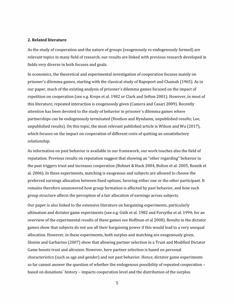
Table 1 summarizes the average contributions, earnings, and cooperation rates in each treatment.

The average contribution was 20.1% in the BT, which is in line with the results of standard Dictator

Game experiments. In the other treatments, the threat of refusing cooperation causes distributors

to raise their contributions to a 30%-40% share, similar to what is observed in Ultimatum Games.

We first turn to Hypothesis 1 (see Table 2). The statistical analysis is performed at the session level

(using session averages), since each session is an independent observation. Average contributions

and receivers' earnings are significantly lower in the BT than in the other treatments (see Tables 2a

and 2c), while distributors' earnings are significantly larger (see Table 2b).

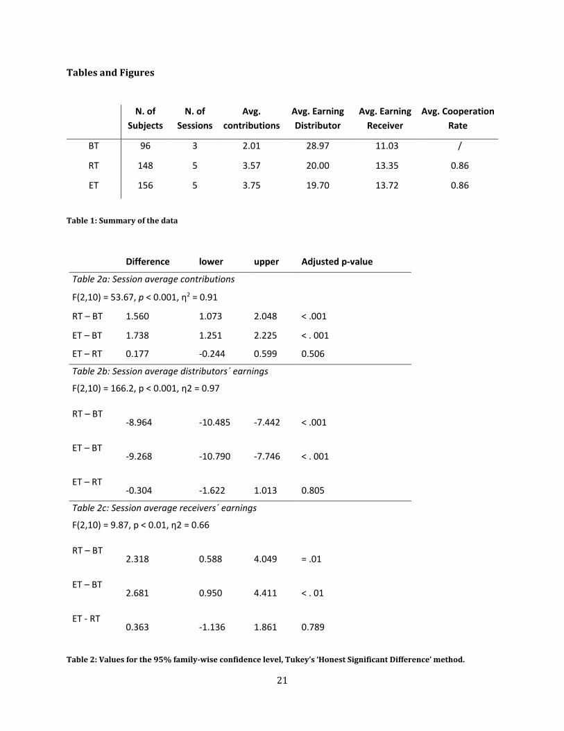
Figure 1 shows the evolution of the average contributions over time in the three treatments. In all

but the last round the contributions were lower in the BT than in the other treatments. To test for

time effects, we compared the sessions´ averages of contributions and earnings of rounds 4 to 13

with those of rounds 20 to 29 for each treatment, excluding the first three rounds, where non-

cooperation was not possible, and the last round, where we observed the well-known “end of the

experiment effect”. No time effect was observed (Paired t-test: BT: t(2) = 0.64, p = 0.59; RT: t(4) =

1.80, p = 0.15; ET: t(4) = 0.40, p = 0.71).

Overall, we can conclude that Hypothesis 1 is supported by the data.

Hypothesis 2 was instead rejected by the data. Tables 2a-c as well as Figure 1 reveal that there is no

significant difference in average contributions and average earnings between the RT and the ET.

Furthermore, average cooperation rates (calculated as the number of times a receiver or a

13

distributor has cooperated, averaged by session) in the RT and the ET are undistinguishable (two

sample t test: t(6.04) = 0, p = 1). However, within the ET treatment we observe substantial

differences in the endogenous life span of groups. In Figure 2, we plot the number of groups with

their duration, weighted by the duration of the group.2 Since during the first three rounds groups

had to cooperate, we take only rounds 4 to 30 into account, implying that the minimum group

duration is 1 and the maximum 27. As can be seen from this figure, 141 groups broke up

immediately since in these cases at least one member of the group refused to cooperate already at

the first round the group was together (groups of duration 1). 41 groups cooperated once and

refused cooperation in the second round of their existence (duration of 2), 30 groups cooperated

twice and refused cooperation in the third round of their existence (duration of 3), etc. Recall that

during these rounds a refusal to cooperate ends the group relationship and the members get

randomly re-matched in the next round (unless they were already in round 30). For example, if a

group was matched in round 15, cooperated from round 15 to round 17, and at least one member

refused to cooperate in round 18, the group duration in that span is 4 rounds.

Overall, Figure 2 reveals a large heterogeneity of group durations, with a lot of short-lived groups,

but also quite some long-term relationships. These differences in group duration translated into

substantial differences in the number of groups subjects belonged to. To see this, we calculated for

each subject the number of groups she or he belonged to during the whole experiment (again

excluding the first three rounds). E.g., if a subject spent 26 rounds with the same group and 1 round

with another group, the number of groups she belonged to is 2. The same results if a subject spent

13 rounds with a group and the remaining 14 round with another group. Figure 3 shows the

distribution of numbers of groups subjects belonged to. Eight distributors and eight receivers were

only members of one group, i.e. four groups (out of 39 possible) stayed together for the whole

experiment. On the other hand, many subjects switched group quite often (e.g. eight distributors

and seven receivers belonged to seven groups), and a few subjects even belonged to more than 20

groups.

2 Weighting by the duration of the group is necessary to avoid misleading results. To see this, take a hypothetical session with 16 subjects and 27 rounds. In this session, half of the subjects stay always in the same group (i.e. two completely stable groups), while the other groups never cooperate and hence always split after one round. In this case we have 2 groups with a duration of 27 rounds each, and 54 groups with a duration of 1. Taking only the number of groups with the different durations would give the impression as if groups of duration 1 would completely dominate the session, while in fact the actual distribution of subjects into the short- and the long-term groups is half/half.

14

These differences in the number of groups subjects belonged to are linked to subjects' behavior.

First, we look at distributors' contributions. As can be seen from Figure 4, distributors' average

contributions differ substantially, ranging from a minimum of 1 to a maximum of 6 ECUs.

Furthermore, Figures 4 suggests a negative correlation between a distributor´s average

contributions and the number of different groups she belonged to, which suggests that groups with

more generous distributors are accepted more frequently. This impression of a negative correlation

between a distributor´s contributions and the number of different groups she belonged to is

confirmed by the statistical analysis (Pearson´s product moment correlation = -.809, t(76) = -12.00,

p < .001). This evidence supports Hypothesis 3i.

Considering that cooperation was nearly never refused by distributors, it follows that receivers

belonging to more groups refuse to cooperate on average more often than receivers belonging to

fewer groups. As already explained, cooperation is driven by (a combination of) two different

factors. First, the higher a receiver's expectation of what to get from a particular pair of

distributors, the more likely she is to cooperate. Since one can expect that distributors' past

contributions are correlated with receivers' expectations about future contributions, higher past

contributions should lead to a larger likelihood of cooperation. Second, for given past contributions

of the distributors, different receivers might differ in their "acceptance" threshold - some receivers

are more seeking than others. To distinguish between these two different reasons for cooperation,

we categorized receivers into three categories of roughly equal size: "Multi-group receivers" who

stayed in at least 9 different, relatively short-lived groups (32 receivers); "few-group receivers"

who stayed in at most 4 different, relatively long-lived groups (24 receivers); and "some-group

receivers" receivers who belonged to a medium number of groups (22 receivers). The thresholds of

four and nine groups were chosen in order to have roughly the same number of subjects in all

categories. To test how past contributions affect cooperation rates in our 3 categories, we do a

probit regression with a cooperation dummy as dependent variable. The average past contributions

(in the last three played rounds) of the distributors and the dummies for the multi-group and the

few-group receivers are the independent variables.

As expected (see Table 3), the likelihood of cooperation increases in the average past contribution

of the distributors (hypothesis 3i). For a given past contribution level, the likelihood of cooperation

is significantly lower for receivers that were in many groups than for those that were in a small or

medium number of groups. We can conclude that receivers who are members of many short-lasting

groups have higher acceptance thresholds than the other receivers, which supports hypothesis 3ii.

15

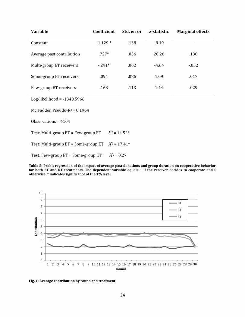
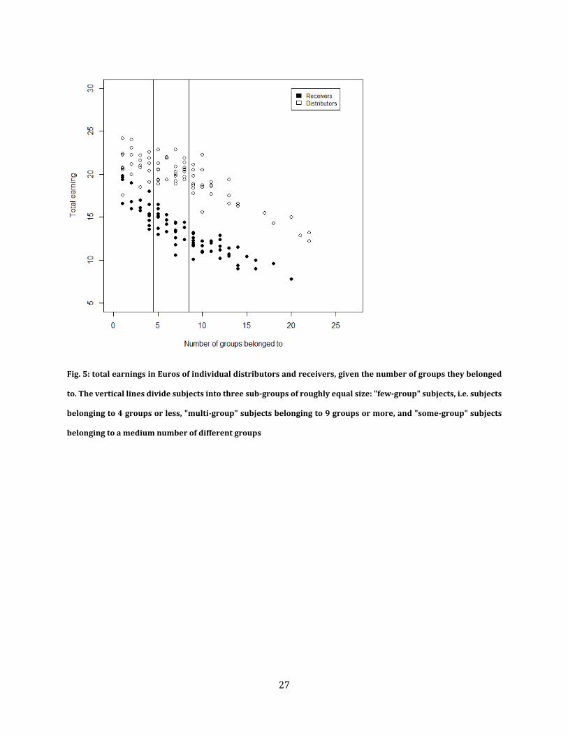
Since receivers belonging to few groups are confronted with distributors contributing more,

receivers' earnings should be negatively correlated with the number of different groups they

belonged to. Concerning distributors' earnings there are two opposing effects at play. On the one

hand, higher contributions have a direct negative effect on distributors' earnings. On the other

hand, higher contributions are connected to fewer groups and more cooperation. Figure 5 indicates

that for distributors too, earnings decrease in function of the number of different groups she

belonged to, showing that the latter effect prevails.

To test for this, we also categorize distributors into "few-group distributors", i.e. distributors

belonging to 4 groups or less (24 distributors), "multi-group distributors" belonging to 9 groups or

more (27 distributors), and "some-group distributors" belonging to a medium number of different

groups (27 distributors). The thresholds of four and nine groups are chosen so to have roughly the

same number of subjects in all categories. Using this categorization of the distributors and the

similar one introduced for receivers above, we find indeed that subjects' earnings are decreasing in

the number of groups they belonged to (receivers: two sample t test, Multi – Few Group, t(38.595) =

12.28, p < .001; distributors: two sample t test, Multi – Few Group, t(43.762) = 6.31, p < .001).

There is also a negative correlation between a subject's earnings and the number of different

groups he/she belonged too (receivers: Pearson’s product-moment correlation = -.936, t(76) = -

18.14, p < .001; distributors: Pearson’s product-moment correlation = -.807, t(76) = -11.95, p <

.001). This confirms Hypotheses 3iii.

Since in the ET we found significant differences between subjects belonging to few and many

groups we compare the behavior of these different ET subjects with the behavior found in the RT.

Table 4 shows that distributors belonging to many groups in the Endogenous treatment contribute

significantly less than RT distributors, whereas those belonging to few ET groups contribute

significantly more. Earnings are larger in the ET than in the RT for both types of subjects whenever

they are in few different groups, and smaller in the ET whenever they are in many different groups.

These differences are all significant.

Concerning cooperation, Table 5 shows the result of a probit regression with the combined data of

the Endogenous treatment and the Re-match treatment. Here the probit regression is run with a

cooperation dummy as dependent variable. The average past contributions of the distributors (in

the last three played rounds) and the dummies for the multi-group, some-group, and the few-group

receivers are the independent variables. Again, higher average past contributions increase the

likelihood of cooperation, and multi-group endogenous treatment receivers have higher acceptance

16

thresholds than few-group and some-group receivers. They have also higher acceptance thresholds

than the average receivers in the Re-match treatment. This is further evidence that the possibility of

staying together leads to self-selection of distributors and receivers.

6. Discussion and Conclusions

This paper investigates the impact of repeated interaction on cooperation levels and surplus

distribution, when group formation is endogenous and ex-post bargaining power differs across

group members. As expected, the opportunity to refuse cooperation restricts the possibility of the

strong agents to take the lion share of the surplus produced by cooperation, leading to more equal

contributions compared to those observed when cooperation is enforced. However, contrary to

what suggested by previous literature and by the folk theorem, we show that repeated interaction

alone does not improve efficiency. Because of the heterogeneity in groups’ behavior, we observe no

impact of the possibility of repeated interaction (endogenous group formation) on the aggregate

contributions and cooperation levels, compared to those observed under exogenous group

formation. Instead, the possibility of repeated interaction with the same partners leads to a self-

selection of agents into groups with different life-spans; long-lived, cooperative groups with high

cooperation levels and contribution rates exist together with short-lived, un-cooperative groups.

The experimental results alone are not able to tell us what drives distributors´ behavior, whether

true generosity or fear of rejection. We are also unable to see how individual differences affect

group duration. In order to answer these questions and to understand why some receivers show

low levels of cooperation, we developed a behavioral model, which we present in Appendix A.

According to our model, the differences in distributors’/receivers’ behaviors are driven by the

different expectations agents have about their partner’s preferences. We suggest that subjects

simply expect others to have the same preferences as they have, and that the amount distributors

decide to offer coincides with the minimum donation they would be willing to accept as receivers.

This implies that distributors that offer the most are those who would be greedy receivers, and that

they act generously for fear of rejection. Similarly, the receivers that accept the lowest amounts

would be greedy distributors, as they would offer a lower amount base on their own acceptance

threshold. Interestingly, our model suggests that the more efficient groups (lasting the longest) are

those composed by modest receivers and greedy distributors, while the groups with the shortest

life-span are those composed by modest distributors and greedy receivers. For tractability, our

model represents the behaviour of pairs, rather than groups of four. However, it nicely reproduces

17

our experimental results and gives interesting insights on the group dynamics, which we believe

hold even for larger groups.

To conclude, our results cast doubts whether the possibility of repeated interaction can

unequivocally lead to cooperative and efficient outcomes when the ex-post bargaining power about

the surplus distribution is very unequal. Rather, it seems to amplify differences in cooperation and

distribution behavior across groups. These results are interesting both from a theoretical and an

applied perspective. Showing that repeated interaction with possibility of punishment (in this case

refusing to cooperate) does not increase efficiency on average is an important result, as well as

observing that the most efficient teams (long-lasting) are not made entirely by other-regarding

members. From a managerial perspective, this gives some insights on the best composition of

groups/teams.

The paper leaves open questions which will be investigated in future research, such as the effect on

cooperation of being matched with distributors with very unequal donations (e.g., one offering the

minimum and one offering a large amount), or the influx of other distributors´ donations on one´s

own donations. Future research will address these points, with a new experimental design

specifically developed to address them.

18

References

Ahn, K., Isaac, M., & Salmon, T. (2008). Endogenous Group Formation. Journal of Public Economic Theory, vol. 10, 171-194.

Alicke, M. D., & Largo, E. (1995). The Role of the Self in the False Consensus Effect. Journal of Experimental Social Psychology, vol.31, 28-47

Baker, G., Gibbons, R., & Murphy, K. (2002). Relational Contracts and the Theory of the Firm. The Quarterly Journal of Economics, Vol. 117, 39-84

Biele, G., Rieskamp, J., & Czienskowski, U. (2008). Explaining cooperation in groups: Testing models of reciprocity and learning. Organizational Behavior and Human Decision Processes.

Bohnet, I., & Huck, S. (2004). Repetition and reputation: Implications for trust and trustworthiness when institutions change. American economic review, 94(2), 362-366.

Bolton, G. E., Katok, E., & Ockenfels, A. (2005). Cooperation among strangers with limited information about reputation. Journal of Public Economics, 89(8), 1457-1468.

Bornstein, G., & Yaniv, I. (1998). Individual and group behavior in the ultimatum game: are groups more “rational” players?. Experimental Economics, 1(1), 101-108.

Camera, G., & Casari, M. (2009). Cooperation among strangers under the shadow of the future. American Economic Review, 99(3), 979-1005.

Chaudhuri, A. (2011). Sustaining cooperation in laboratory public goods experiments: a selective survey of the literature. Experimental economics, 14(1), 47-83.

Cinyabuguma, M., Page, T., Putterman, L. (2005). Cooperation Under the Threat of Expulsion in a Public Goods Experiment. Journal of Public Economics, vol. 89, 1421-35.

Clark, K., & Sefton, M. (2001). The Sequential Prisoner's Dilemma: Evidence on Reciprocation. Economic Journal, vol. 111, 51-68.

Cooper, D., & Kagel, J. H. (2016). Other-Regarding Preferences: A Selective Survey of Experimental Results. In Kagel, J. H. & Roth, A. (eds.), The Handbook of Experimental Economics, Volume 2 (pp. 217-289). Princeton University Press.

Coricelli, G., Fehr, D., & Fellner, G. (2004). Partner selection in public goods experiments. Journal of Conflict Resolution, 48(3), 356-378.

Dawes, R. M., McTavish, J., & Shaklee, H. (1977). Behavior, Communication and Assumptions About Other People´s Behavior in a Commons Dilemma Situation. Journal of Personality and Social Psychology, vol.35, 1-11

Debove, S., André, J., & Baumard, N. (2015). Partner choice creates fairness in humans. Proceedings of the Royal Society B, DOI: 10.1098/rspb.2015.0392

Ellison, G. (1994). Cooperation in the Prisoner's Dilemma with Anonymous Random Matching. The Review of Economic Studies, vol.61, 567-588

Fehrler, S., & Przepiorka, W. (2016). Choosing a partner for social exchange: Charitable giving as a signal of trustworthiness. Journal of Economic Behavior & Organization, 129, 157-171.

19

Forsythe, R., Horowitz, J., Savin, N., & Sefton, M. (1994). Fairness in simple bargaining experiments. Games and Economic Behavior, vol 6, 347-369.

Fu, T., Ji, Y., Kamei, K., & Putterman, L. ( ). Punishment can support cooperation even when punishable. Economics Letters, 154, 84-87.

Fudenberg, D., & Maskin, E. (1986). The Folk Theorem in Repeated Games with Discounting or with Incomplete Information. Econometrica, Vol. 54, 533-554

Fung, J. M., & Au, W. T. (2014). Effect of inequality on cooperation: heterogeneity and hegemony in public goods dilemma. Organizational Behavior and Human Decision Processes, 123(1), 9-22.

Gächter, S., & Thöni, C. (2005). Social learning and voluntary cooperation among like-minded people". Journal of the European Economic Association, vol. 3, 303-314.

Gaudeul, A., Crosetto, P., & Riener, G. (2017). Better stuck together or free to go? Of the stability of cooperation when individuals have outside options. Journal of Economic Psychology, 59, 99-112.

Gehrig, T., Güth, W., Levati, V., Levinsky, R., Ockenfels, A., Uske, T., & Weiland, T. (2007). Buying a pig in a poke: An experimental study of unconditional veto power. Journal of Economic Psychology, 28(6), 692-703.

Güth, W., & Kirchkamp, O. (2012). Will you accept without knowing what? The Yes-No game in the newspaper and in the lab. Experimental Economics, 15(4), 656-666.

Güth, W., Schmittberger, R., & Schwarz, B. (1982). An experimental analysis of ultimatum bargaining. Journal of Economic Behavior and Organization, vol. 3, 367-388.

Hoffman, E., McCabe, K., & Smith, V. (2008). Reciprocity in Ultimatum and Dictator Games: An Introduction. Chap. 46 in C. Plott and V. Smith (eds.), Handbook of Experimental Economic Results, North Holland

Kreps, D., Milgrom, P., Roberts, J., & Wilson, R. (1982). Rational cooperation in the finitely repeated prisoners' dilemma. Journal of Economic Theory, vol. 27(2), 245–252.

Mullen, B., Atkins, J. L., Champion, D. S., Edwards, C., Hardy, D., Story, J. E., & Vanderklok, M. (1985). The false consensus effect: A meta-analysis of 115 hypothesis tests. Journal of Experimental Social Pshychology, vol.21, 262-283

Page, T., Putterman, L., & Unel, B. (2005). Voluntary Association in Public Goods Experiments: Reciprocity, Mimicry, and Efficiency. Economic Journal, vol. 115, 1032-53.

Rapoport, A., & Chammah, A. (1965). Prisoner's Dilemma: A Study in Conflict and Cooperation, University of Michigan Press

Resnick, P., Zeckhauser, R., Swanson, J., & Lockwood, K. (2006). The value of reputation on eBay: A controlled experiment. Experimental economics, 9(2), 79-101.

Robbins, J. M., & Krueger, J. I. (2005). Social Projection to Ingroups and Outgroups: A Review and Meta-Analysis. Personality and Social Psychology Review, vol. 9, 32-47

Slonim, R., & Garbarino, E. (2008). Increases in trust and altruism from partner selection: Experimental evidence. Experimental Economics, vol. 11, 134–153.

20

Wilson, A. J., & Wu, H. (2017). At-will relationships: How an option to walk away affects cooperation and efficiency. Games and Economic Behavior, 102, 487-507.

21

Tables and Figures

N. of

Subjects N. of

Sessions Avg.

contributions Avg. Earning Distributor

Avg. Earning Receiver

Avg. Cooperation Rate

BT 96 3 2.01 28.97 11.03 /

RT 148 5 3.57 20.00 13.35 0.86

ET 156 5 3.75 19.70 13.72 0.86

Table 1: Summary of the data

Difference lower upper Adjusted p-value

Table 2a: Session average contributions

F(2,10) = 53.67, p < 0.001, η2 = 0.91

RT – BT 1.560 1.073 2.048 < .001

ET – BT 1.738 1.251 2.225 < . 001

ET – RT 0.177 -0.244 0.599 0.506

Table 2b: Session average distributors´ earnings

F(2,10) = 166.2, p < 0.001, η2 = 0.97

RT – BT

-8.964

-10.485

-7.442

< .001

ET – BT

-9.268

-10.790

-7.746

< . 001

ET – RT

-0.304

-1.622

1.013

0.805

Table 2c: Session average receivers´ earnings

F(2,10) = 9.87, p < 0.01, η2 = 0.66

RT – BT

2.318

0.588

4.049

= .01

ET – BT

2.681

0.950

4.411

< . 01

ET - RT

0.363

-1.136

1.861

0.789

Table 2: Values for the 95% family-wise confidence level, Tukey’s ‘Honest Significant Difference’ method.

22

Variable Coefficient Std. error z-statistic Marginal effects

Constant -.567* .168 -3.37 -

Average past contribution .553* .046 12.02 .101

Few-group dummy .175 .129 1.36 .032

Multi -group dummy -.444* .091 -4.88 -.081

Log-likelihood = -702.93947

Mc Fadden Pseudo-R2 = 0.1947

Observations = 2106

Test: Multi -group = Few-group, Χ2 = 26.61*

Table 3: Probit regression of the impact of average past contributions and number of groups a receiver belonged to on cooperative behavior. The dependent variable equals 1 if the receiver decides to cooperate and 0 otherwise. * indicates significance at the 1% level.

23

Difference lower upper Adjusted p-value

Table 4a: Comparison of distributors´ contributions

F(2,123) = 26.57, p < 0.001, η2 = 0.30

Multi-group ET – Few-group ET

-1.505 -2.056 -0.953 0.000

Re-match tr. – Few-group ET

-.901 -1.362 -0.439 0.000

Re-match tr. – Multi-group ET

0.604

0.162

1.045

0.004

Table 4b: Comparisons of distributors´ earnings

F(2,122) = 23.55, p < 0.001, η2 = 0.278

Multi-group ET – Few-group ET

-3.704 -5.036 -2.372 0.000

Re-match tr. – Few-group ET

-1.275

-2.390

-0.159

0.020

Re-match tr. – Multi-group ET

2.472

1.362

3.497

0.000

Table 4c: Comparisons of receivers´ earnings

F(2,127) = 102.3, p < 0.001, η2 = 0.617

Multi-group ET – Few-group ET

-5.693 -6.641 -4.746 0.000

Re-match tr. –

Few-group ET

-3.568

-4.392

-2.274

0.000

Re-match tr. – Multi-group ET tr.

2.124

1.382

2.867

0.000

Table 4: Values for the 95% family-wise confidence level, Tukey’s ‘Honest Significant Difference’ method. For RT we used the contributions/the total earnings of all distributors/subjects (distributors: 74, receivers: 74) of the RT; for the multi-group ET the contributions/total earnings of all distributors/subjects that were in at least 9 groups (distributors: 27, receivers: 32), and for few-group ET the contributions/total earnings of all of all distributors/subjects that had were in at most 4 groups for both (distributors: 24, receivers: 24).

24

Variable Coefficient Std. error z-statistic Marginal effects

Constant -1.129 * .138 -8.19 -

Average past contribution .727* .036 20.26 .130

Multi-group ET receivers -.291* .062 -4.64 -.052

Some-group ET receivers .094 .086 1.09 .017

Few-group ET receivers .163 .113 1.44 .029

Log-likelihood = -1340.5966

Mc Fadden Pseudo-R2 = 0.1964

Observations = 4104

Test: Multi-group ET = Few-group ET Χ2 = 14.52*

Test: Multi-group ET = Some-group ET Χ2 = 17.41*

Test: Few-group ET = Some-group ET Χ2 = 0.27

Table 5: Probit regression of the impact of average past donations and group duration on cooperative behavior, for both ET and RT treatments. The dependent variable equals 1 if the receiver decides to cooperate and 0 otherwise. * indicates significance at the 1% level.

Fig. 1: Average contribution by round and treatment

0

1

2

3

4

5

6

7

8

9

10

1 2 3 4 5 6 7 8 9 10 11 12 13 14 15 16 17 18 19 20 21 22 23 24 25 26 27 28 29 30

Cont

ribu

tion

Round

BT

RT

ET

25

Fig. 2: For each possible duration of a match, how many groups stick together for that amount of rounds times the

duration of the match

Fig. 3: How many subjects belonged to a specific number of groups during the experiment

141

8290

56 6054

4956

36

10

22 24 26

56

15 16 18 20

42

23 24 25

108

0

20

40

60

80

100

120

140

160

1 2 3 4 5 6 7 8 9 10 11 12 13 14 15 16 17 18 19 20 21 22 23 24 25 26 27

Num

ber

of g

roup

s of

a c

erta

in d

urat

ion

* du

rati

on

Group duration

8

5

6

5

8

3

8 8

7

5

4

3

2

1 1 1 1 1

8

4

3

9

8

4

7

3

9

4

3

5

3 3

1

2

1 1

0

1

2

3

4

5

6

7

8

9

10

1 2 3 4 5 6 7 8 9 10 11 12 13 14 15 16 17 18 19 20 21 22

Num

ber

of s

ubje

cts

Number of groups a subject belonged to

Distributors

Receivers

26

Fig. 4: average contribution of individual distributors, given the number of groups she belonged to. The vertical

lines divide distributors into three sub-groups of roughly equal size: "few-group distributors", i.e. distributors

belonging to 4 groups or less (24 distributors), "multi-group distributors" belonging to 9 groups or more (27

distributors), and "some-group distributors" belonging to a medium number of different groups (27 distributors)

27

Fig. 5: total earnings in Euros of individual distributors and receivers, given the number of groups they belonged

to. The vertical lines divide subjects into three sub-groups of roughly equal size: "few-group" subjects, i.e. subjects

belonging to 4 groups or less, "multi-group" subjects belonging to 9 groups or more, and "some-group" subjects

belonging to a medium number of different groups

28

Electronic Supplementary Material

Endogenous Group Formation and its impact on Cooperation and Surplus Allocation - An Experimental Analysis

Sibilla Di Guida, The Anh Han, Georg Kirchsteiger, Tom Lenaerts, and Ioannis Zisis

29

Appendix A:

A behavioral model

In our paper, we have observed that contributions and cooperation rates do not differ on average in

ET and RT. We have also seen that in ET agents self select into groups whose life spans differ largely

and that receivers´ expectations have a large impact on their cooperation rates. What we are not able

to understand from the experimental data is what drives distributors to contribute differently and

how individual differences affect group duration. In order to explain the qualitative features of the

experimental results, we have developed a behavioral model. To keep the analysis simple, we

investigate a variant of the surplus allocation game with one receiver and one distributor forming a

group, and with only receivers deciding about cooperation. More specifically, the following 2-stage

game is played repeatedly: First, receivers decide whether to cooperate or not (choices "y" or "n"). If

a receiver refuses to cooperate, no surplus is produced and both group members earn nothing in that

round. In case of cooperation, a surplus of 10 is produced. In the second stage of the game the

distributor decides unilaterally about her contribution "c" to the payoff of "her" receiver. The set of

feasible contributions is given by C={1,2,..10}. Hence, the earnings of the receivers and distributors,

xr and xd, in round t are given by

xrt(y,c)=c, xdt(y,c)=10-c, and xrt(n,.)=xdt(n,.)=0.

To allow for informed cooperation decisions, each receiver is informed about the previous

contribution of "his" distributors, cp, before the decision about cooperation is taken. Overall, this

game is played for T rounds. In the first round, cooperation is enforced, and only the distributor has

to decide about the contribution (i.e. the first round is a dictator game). Hence, a cp exists for every

distributor in every round where the receivers make cooperation decisions, i.e. in all t>1.

As in the experiment, we analyse two different matching protocols: In the re-match (RT), from round

two onwards, subjects get re-matched every round using independent draws. With endogenous

matching (ET) each group stays together until the receiver stops cooperating, in which case the

agents get randomly re-matched with other agents unmatched in the respective round. We also look

at the case where cooperation is exogenously enforced and agents get re-matched every round (BT).

The model is based on three straightforward behavioural assumptions.

1) Each agent (distributors and receivers) is endowed with an acceptance threshold c̃ that denotes

the minimum previous contribution such that the particular agent would cooperate if he played the

role of a receiver. This cooperation threshold describes the actual behavior of each receiver - if cp≥c̃,

30

the receiver cooperates, otherwise he refuses cooperation (but for the possibility of making mistakes

- see point 3 below). A distributor’s cooperation threshold impacts her beliefs about the cooperation

thresholds of the matched receiver (see point 2 below), which in turn is crucial for the optimal

contribution of the distributor.

Agents differ in their acceptance thresholds. More specifically, there exist two types of agents in the

population. Both receivers and distributors can be either modest (type m) or seeking (type s). Overall

there is a mass of 1 of each receivers and distributors, and a fraction g of both of them is of type m.

By definition, c̃s>c̃m, and we assume that 5≥c̃s>c̃m≥1- both types of receivers cooperate with someone

who previously contributed half of the surplus.

2) Each distributor wants to make choices that maximize the sum of the earnings of all rounds.

Denote by c*(τ,t) the optimal choice of a distributor of type τ in round t for given distributor's belief

about the receivers' types. To determine c*(τ,t), the distributor has to take the impact of her choices

on the future cooperation behavior of her receivers into account, which of course depend on the types

of the future receivers (see point 1 above).

To model the distributors' beliefs about the receivers' types we start from the observation that

humans think that their own types are more present in the general population than they actually are.

Because of the evidence cited in the introduction, we assume that in all rounds each contributor

believes with certainty that all receivers are of her own type. This assumption is consistent with

Bayesian updating when each distributor has the prior belief that all receivers are of her own type,

provided that the receivers make mistakes when deciding about cooperation (see point 3 below).

Within such a model, any cooperation decision contradicting the distributor's a-priori belief would

be regarded as a mistake, leaving the beliefs about the receiver's type unchanged. This assumption is

consistent with the experimental result that differences in distributor's choices remained stable

during the experiment except for the very last round, implying that indeed little if any belief updating

took place during the course of the experiment.

3) Whenever a choice is made, each receiver and each distributor makes a mistake with probability

α, 0<α<1/2. For a type-τ receiver this implies that the likelihood of cooperation is (1-α) if cp≥ c̃τ, and

α otherwise.

In case of a mistake, a distributor chooses a contribution according to a probability distribution with

full support on the set of feasible contributions. We assume that this probability distribution depends

on her intended choice c*. Denote by p(c|c*) the likelihood that c is chosen in case of a mistake, if the

distributor intends c*. The resulting cumulative probability distribution is P(c|c*), i.e. P(c|c*) is the

31

likelihood that the actually chosen contribution is weakly below c in case of a mistake, if the

distributor intends c*. We assume that the distributor is less likely to pick a small contribution if he

intends to choose a relatively high contribution than if he intends a low contribution. Formally, for

all c, c*, and c*' with c*<c*' and c<10, P(c|c*)> P(c|c*').

Taking into account that mistakes occur with a probability of α, the likelihood that the actual choice

c is equal to the intended choice c* is (1-α)+αp(c*|c*). The likelihood of a choice c≠c* is given by

αp(c|c*). Likewise, the likelihood that the actual choice is weakly below a certain level c is given by

αP(c|c*) if c< c*, and it is (1-α)+αP(c|c*)] if c≥c*.

Using this framework, we get the following results (see proofs below):

Proposition 1:

i) In the BT, c*(τ,t)=1 for both types τ=m,s for all rounds.

ii) If the receiver cooperated in the last round T, the optimal intended contribution c*(τ,T)=1 for both

types τ=m,s in the RT as well as in the ET.

iii) For α small enough and for any round t with t<T it holds: If the receiver cooperated, the optimal

intended contribution of the distributor is given by c*(τ,t)= c̃τ for both types τ=m,s in the RT as well

as in the ET.

Proposition 1 shows that the contribution is lower in BT than in ET and RT, as observed in the

experiment. In the ET and RT a distributor, who would be seeking (s-type) in case she were a receiver,

contributes more than someone who thinks all agents (including herself) are modest, provided that

the mistake probability is small enough. Hence, an s-type distributor appears more generous than m-

types, not because of real generosity, but due to the fear that without generosity receivers refrain

from cooperating with her.

From now on we assume that the mistake probability is small enough that Proposition 1iii holds.

Next we turn to the likelihood of cooperation. Since the likelihood of cooperation depends on the

previous contribution of the distributor, and on the type of the receiver, it depends on the group

composition. Denote by prob(y|τd,τr) the probability of cooperation when the group is formed of a d-

type distributor and a r-type receiver. We get:

Proposition 2: In the ET and the RT it holds that groups consisting of a seeking distributor and a

modest receiver have the highest cooperation probabilities, while groups consisting of a modest

distributor and a seeking receiver have the lowest cooperation probabilities:

32

i) prob(y|τd=s; τr=m) > prob(y|τd=τr=m) and prob(y|τd=s; τr=m) > prob(y|τd=τs=s), and

ii) prob(y|τd=τr=m) > prob(y|τd=m;τr=s) and prob(y|τd=τs=s) > prob(y|τd=m;τr=s).

Note that prob(y|τd=τr=m) > prob(y|τd=m;τr=s) and prob(y|τd=s; τr=m) > prob(y|τd=τr=s) - an m-

type receiver is more likely to cooperate than an s-type for any given type of distributor he can be

matched with. Hence, the expected cooperation rates are larger for m-type than for s-type receivers.

Similarly, prob(y|τd=s; τr=m) > prob(y|τd=τr=m) and prob(y|τd=τr=s) > prob(y|τd=m;τr=s) - an s-

type distributor experiences more cooperation than an m-type for any given type of receiver she can

be matched with. Hence, in expectations the experienced cooperation rates are larger for s-type

distributors than for m-type distributors, and for m-type receivers than for s-type receivers.

Furthermore, for the ET Proposition 2 implies that groups consisting of a modest receiver and a

seeking distributor have the longest expected duration, whereas groups consisting of a seeking

receiver and a modest distributor have the shortest expected duration.

Proposition 1 states the intended contributions of the different types of distributors in the ET and

the RT provided that the receivers have cooperated. But not all groups cooperate, and for a given

group the probability of cooperation depends on the types of the receiver and the distributor, i.e. on

the type composition of the respective group (Proposition 2). To calculate the overall cooperation

rate in the population, and the average contribution level, we have to take into account how often the

four different possible type combinations are present in the population. This leads to the following

Proposition 3: For α converging to zero, the observed cooperation rates and the observed

contributions converge to the same level in the ET and the RT treatment. For α=0 the following holds:

i) In both treatments the cooperation rate is 1-g(1-g) in any round but round 1.

ii) In both treatments, a mass of (1-g) distributors choose a contribution of c̃s, a mass of g2

distributors chooses c̃m, and the other distributors do not have to make a contribution choice in any

round but round 1 since their receivers do not cooperate.

According to Proposition 3, average observed cooperation and contribution behavior are similar in

both treatments as long as the mistake rates are not too large. Furthermore, in the ET there is a large

variance in the number of groups an agent belongs to, and the contribution of a distributor as well as

the acceptance threshold of a receiver are correlated with the number of groups (s)he belongs to:

Proposition 4: When α converges to zero the following holds:

i) In the ET, a fraction of g(1-g) receivers and distributors are members of T groups, while all other

receivers are members of only 1 group.

33

ii) The average contribution of a multi-group ET distributor is below the average contribution of an

RT distributor, while the average contribution of a few-group ET distributor is larger than that of an

RT distributor.

iii) The average acceptance threshold of an RT receiver is below the average acceptance threshold of

a multi-group ET receiver, and above that of an few-round ET receiver.

Proposition 4 is in accordance with the experimental results. With respect to the payoffs we get the

following result:

Proposition 5: For α=0 it holds:

i) The average payoff of the distributors is larger in the BT than in the two other treatments. The

average payoff of the receivers is smaller in the BT than in the two other treatments.

ii) The average payoffs of distributors and receivers are the same in the RT and the ET.

iii) Few-group ET agents have higher expected payoff than RT agents, who in turn have higher payoff

than multi-group ET agents.

Again, this proposition reflects the results found in the experiment.

To summarize, the model captures the main experimental results very well: In the BT, contributions

are smaller than in the other treatments, leading to higher distributors' payoffs and lower

receivers' payoffs in the BT than in the other treatments. On average, cooperation rates,

contribution levels, and earnings are the same in the ET and the RT. However, in ET group

durations differ, and so does the number of groups each particular agent is member of. Multi-group

ET receivers cooperate less than RT receivers, while few-group ET receivers cooperate more. And

multi-group ET distributors contribute less than RT receivers, while few-group ET distributors

contribute more. Furthermore, the resulting payoff structure is in accordance with the

experimental results. The model also sheds light on the rationales that drive distributors/receivers

to behave in different ways and self-select. Seeking distributors are those who contribute more, not

driven by true generosity, but by fear of rejection. The more efficient groups (lasting the longest)

are those composed by modest receivers and seeking distributors, while the groups with the

shortest life-span are those composed by modest distributors and seeking receivers.

Proof of Proposition 1

34

i and ii) In the BT, in any round t any increase in the contribution unambiguously decreases the

overall payoff of the distributor. The same argument holds for the last round T in the other

treatments.

iii) First note that in any round for a given previous contribution the cooperation probability is

continuous in α. Furthermore, for given cooperation decision and given intended contribution the

expected contribution is continuous in α. Hence, in any given round the expected earnings of this

round are continuous in α.

Next we show that in any round t<T with zero mistake probabilities the sum of a type τ-distributor's

earnings in all rounds weakly larger than t is strictly larger when he chooses a contribution of c̃τ in

round t than when he chooses any other distribution in round t, given his belief that all receivers are

also of type τ. Since this holds for any t<T and since earnings are continuous in α, it is optimal to

choose c*(τ,t)= c̃τ in all rounds but T for small enough α.

Take round T-1 and α=0. A distributor of type τ has to distribute a surplus (i.e. her receiver in round

T-1 decided to cooperate). We have to distinguish between two sets of choices (since α=0, the

intended choice equals the actual choice). First, we look at all choices c<c̃τ. In this case the

distributor's expected earnings of the last two rounds are given by xd(T-1)+ xdT=10-c, since the

distributor expects that in the last round the receiver will not cooperate. Hence, within the set of

choices c<c̃τ the earnings are maximized at c=1, leading to xd(T-1)+ xdT=9.

Second, we look at all choices c≥c̃τ. In this case her expected earnings of the last two rounds are given

by xd(T-1)+ xdT =10-c+9, since the distributor expects that in the last round the receiver will cooperate

and she will earn 9 in the last round. Hence, within the set of choices c≥c̃τ the earnings are maximized

at c= c̃τ leading to xd(T-1)+ xdT=10-c̃τ +9. Obviously, these earning are strictly larger than the maximum

the distributor could earn during the last two rounds with any c<c̃τ. Therefore, the unique earning

maximizing choice of the distributor in round T-1 is given by c*(τ,T-1)= c̃τ, and by continuity of the

earning function this holds true for small enough α.

Next, take round T-2 and α=0 with a distributor of type τ having to distribute a surplus (i.e. her

receiver in round T-2 decided to cooperate). Again, we have to distinguish between two sets of

choices (since α=0, the intended choice equals the actual choice). First, we look at all choices c<c̃τ. In

this case the distributor's expected earnings of the last three rounds are given by xd(T-2)+xd(T-1)+

xdT=10-c, since the distributor expects that in the last 2 rounds the receivers will not cooperate.

Hence, within the set of choices c<c̃τ the earnings are maximized at c=1, leading to xd(T-1)+ xdT=9.

35

Second, we look at all choices c≥c̃τ. In this case her expected earnings of the last three rounds are

given by xd(T-2)+xd(T-1)+ xdT=10-c+(10- c̃τ)+9, since the distributor expects that in round T-1 the

receivers will cooperate and she will chooses c*= c̃τ, leading cooperation in round T. Hence, the

distributor will earn (10- c̃τ) and 9, respectively, in the last 2 rounds. Within the set of choices c≥c̃τ

the earnings are maximized at c= c̃τ , leading to xd(T-2)+xd(T-1)+ xdT = 2(10-c̃τ)+9.

These earnings are strictly larger than the maximum the distributor could earn during the last three

rounds with any c<c̃τ. Therefore, the unique earning maximizing choice of the distributor in round

T-2 is given by c*(τ,T-2)= c̃τ, and by continuity of the payoff-function this holds for small enough α.

The same proof goes through for any round t<T-2. Within the set of choices c<c̃τ the earning

maximizing choice is 1, implying expected earnings for the last T-t+1 rounds of Σn≥txdn = 9. Within

the set of choices c≥c̃τ the earning maximizing choice is c̃τ, implying expected earnings for the last T-

t+1 rounds of Σn≥txdn = (T-t)(10-c̃τ)+9, which is strictly larger than 9. Therefore, for all rounds t<T

the earning maximizing contribution is given by c*(τ,t)= c̃τ for a small enough mistake probability.

Note that this proof also holds for t=1 when cooperation is enforced, i.e when a dictator game is

played.

Proof of Proposition 2

Since round 1 is a dictator game, at least one previous round exists where the distributor made a

choice. In this previous round, she intended to choose c*=c̃τ, since this is her intention in all rounds

but T (obviously, T can never be the previous round). Since the intended previous choice only

depends on the type of the distributor, the probability distribution of the actual previous choices

depends only on the distributor's type. Since the cooperation decision of the receivers depends only

on the previous choice and on the type of the receiver, the likelihood of cooperation depends only on

the pair of types. We have groups with 4 different type combinations:

Case a) Receiver and distributor are of type m, i.e. τr=τd=m. Because the distributor intended c̃τ=c̃m

in the previous round, the likelihood of an actual previous choice cp<c̃m is given by

prob(cp|c<c̃m)=αP(c̃m-1|c̃m), while the likelihood that the actual previous choice cp is weakly larger

than c̃m is given by prob(cp|c≥c̃m)=1-αP(c̃m-1|c̃m). This implies a cooperation probability of

prob(y|τd=τr=m) = α2P(c̃m-1|c̃m)+(1-α)[1-α P(c̃m-1|c̃m)]=1-α-α(1-2α)P(c̃m-1|c̃m).

Case b) τr=τd=s. This is exactly the same as Case 1, except that P(c̃m-1|c̃m) has to be replaced by P(c̃s-

1|c̃s). Hence prob(y|τd=τs=s)=1-α-α(1-2α)P(c̃s-1|c̃s).

36

Case c) τd=s; τr=m. Because the distributor intended c̃s in the previous round, and because c̃m< c̃s,

the likelihood of an actual previous choice cp<c̃m is given by prob(cp|c<c̃m)=αP(c̃m-1|c̃s), while the

likelihood that the actual previous choice cp is weakly larger than c̃m is given by prob(cp|c≥c̃m)=1-

αP(c̃m-1|c̃s). This implies a cooperation probability of

prob(y|τd=s; τr=m)= α2P(c̃m-1|c̃s)+(1-α)[1-αP(c̃m-1|c̃s)]=1-α-α(1-2α)P(c̃m-1|c̃s).

Case d) τd=m;τr=s. Because the distributor intended c̃m in the previous round, and because c̃m< c̃s

the likelihood of an actual previous choice cp <c̃s is given by prob(cp|c<c̃s)= (1-α)+αP(c̃s-1|c̃m), while

the likelihood that the actual previous choice cp is weakly larger than c̃f is given by

prob(cp|c≥c̃s)=α[1-P(c̃s-1|c̃m)].This implies a cooperation probability of

prob(y|τd=m;τr=s)=α[(1-α)+αP(c̃s-1|c̃m)]+(1-α)[α[1-P(c̃s-1|c̃m)]]=2α(1-α)-α(1-2α)P(c̃s-1|c̃m).

Recall that P(.|c̃s) and P(.|c̃m) are cumulative distributions derived from a full support distributions.

Therefore, P(c̃s-1|c̃s)>P(c̃m-1|c̃s) and P(c̃s-1|c̃m)>P(c̃m-1|c̃m) since c̃s-1>c̃m-1. This implies that

prob(y|τd=s; τr=m)=1-α-α(1-2α)P(c̃m-1|c̃s) > 1-α-α(1-2α)P(c̃s-1|c̃s)= prob(y|τd=τs=s), and

prob(y|τd=τr=m)=1-α-α(1-2α)P(c̃m-1|c̃m) > 2α(1-α)-α(1-2α)P(c̃s-1|c̃m)= prob(y|τd=m;τr=s).

By assumption P(c̃m-1|c̃m)>P(c̃m-1|c̃s) and P(c̃s-1|c̃m)>P(c̃s-1|c̃s). Hence,

prob(y|τd=s; τr=m)=1-α-α(1-2α)P(c̃m-1|c̃s) > 1-α-α(1-2α)P(c̃m-1|c̃m)=prob(y|τd=τr=m), and

prob(y|τd=τs=s)=1-α-α(1-2α)P(c̃s-1|c̃s) > 2α(1-α)-α(1-2α)P(c̃s-1|c̃m)= prob(y|τd=m;τr=s).

Proof of Proposition 3

First, we look at the ET. In any round for a given previous contribution the cooperation probability is

continuous in α. Furthermore, for given cooperation decision and given intended contribution the

expected contribution is continuous in α. Hence, the distribution of group compositions in the next

round is continuous in α.

Take α=0, and look at the first round. In this round, where cooperation is exogenously enforced, a

fraction g of distributors chooses a contribution of c̃m, and a fraction of (1-g) distributors chooses c̃s.

In the round 2, we have a fraction of g(1-g) groups that consist of a m-type distributor and a s-type

receiver. In these groups the receivers do no cooperate, since their distributors have chosen c̃m in

round 1 and they require at least a previous contribution of c̃s to cooperate. These groups get

immediately split up again.

37

In the round 2, we also have a fraction of (1-g)g groups that consist of a s-type distributor and a m-

type receiver. In these groups the receivers cooperate, the distributors contribute c̃s, and the groups

stay together in round 3. For the fraction (1-g)2 groups consisting of τd=τr=s the receivers cooperate,

the distributors contribute c̃s, and the groups stay together in round 3. Similarly, for the fraction g2

groups consisting of τd=τr=m the receivers cooperate, the distributors contribute c̃m, and the groups

also stay together in round 3.

In round 3, all agents stay with their previous partners except a mass of (1-g)g of s-type distributors

and the same mass of m-type receivers. These distributors and receivers - coming from a

(τd=m,τr=s)-group - get re-matched, but with a partner of the same type as they experienced in round

2. Hence, these receivers will again not cooperate, and these groups will again be split up. All other

round-2- groups remain together also in round 3, the receivers cooperate, the distributors contribute

according to their types, and the group stay together also in round 4. By applying the same logic to

all the following rounds, these groups will stay together for the rest of the game, while the

distributors and receivers coming from a split-up (τd=m,τr=s)-group will never cooperate again.

Hence, the rate of non-cooperation is (1-g)g for all rounds of the ET treatment (except for round 1).

Furthermore, in any round but the first one (1-g) distributors choose a contribution of c̃s, g2

distributors choose c̃m, and g(1-g) distributors do not have to make a distribution choice since their

receivers do not cooperate.

For the RT, note a group cooperates except if it is composed of τd=s,τr=m. Due to law of larger

numbers and since groups are composed according by random and independent draws, τd=s,τr=m

groups are formed in (1-g)g cases, like in the ET. The rate of non-cooperation in the RT is (1-g)g like

in the ET, and the contributions are c̃s for (1-g) distributors and c̃m for g2 distributors, again like in

the ET.

Proof of Proposition 4

i) It follows immediately from the proof of Proposition 3, a fraction of g(1-g) ET receivers an

distributors are members of T groups, while all others ET receivers stay in the same group all the

rounds (Recall that in round 1 where cooperation is exogenously enforced).

ii) A multi-round ET distributors choose 0 except for round. The few-round ET distributors consist

of a mass of (1-g) agents contributing c̃s and g2 agents contributing c̃m in all rounds. Hence, the

average contribution of a few-round ET distributor is [(1-g)c̃s+g2c̃m]/[1-g+g2]. In the RT (1-g)

38

distributors contribute c̃s, g2 contribute c̃m, and the rest nothing. Hence, the average contribution in

the RT is given by (1-g)c̃s+g2c̃m.

iii) The average acceptance threshold of an RT receiver is gc̃m+(1-g)c̃s. For multi-round receiver it is

c̃s, while for a few-round ET receiver it is gc̃m+(1-g)2c̃s.

Proof of Proposition 5

ii) In round 1, when cooperation is enforced, g distributors choose c̃m and (1-g) distributors choose

c̃s in all rounds. As can be seen from the proof of proposition 3, the same groups are formed in all

later in both treatments, leading to the same cooperation and contribution behavior. Hence, the

average payoffs are the same in both treatments.

i) Since distributors always receive the maximum possible payoff, namely 9, in every round of the BT,

and since in the ET and the RT a mass of g(1-g) distributors faces non-cooperation in all rounds, The

distributors' payoffs are strictly larger in the BT than in the RT and the ET.

Receivers get an expected payoff of (1-g)c̃s+g2c̃m in every round, and since c̃s>c̃m≤2 and 1>g>0, it

holds that (1-g)c̃s+g2c̃m>1, which is the payoff receivers get in the every round of the BT.

iii) Multi-group ET receivers do not cooperate in any round, and multi-group distributors do not

experience cooperation but for round 1 when cooperation is exogenously enforced. Hence, the

payoffs of these agents are below that of few-round agents who are in groups that always cooperate.

Because of i this also implies that the payoffs of RT agents must be in between those of multi-group

ET and few-group ET agents.

39

Appendix B:

Experimental Instructions

Base treatment (BT)

Dear Participant, welcome!

You are about to participate in an experiment on interactive decision-making, conducted by

researchers from the Vrije Universiteit Brussel and the Université Libre de Bruxelles, and funded by

the Belgian fund for the scientific research (Fonds de la Recherche Scientifique). In this experiment

you will earn some money, and the amount will be determined by your choices and by the choices of

the other participants.

Your privacy is guaranteed: all results will be used anonymously.

It is very important that you remain silent during the whole experiment, and that you never

communicate with the other participants, neither verbally, nor in any other way. For any doubts or

problems you may have, please just raise your hand and an experimenter will approach you. If you

do not remain silent or if you behave in any way that could potentially disturb the experiment, you

will be asked to leave the laboratory, and you will not be paid.

All your earnings during the experiment will be expressed in Experimental Currency Units (ECUs),

which will be transformed into Euros with a change rate of 10 to 1. At the end of the experiment, a

show up fee of 2.5 euros will be added to your earnings.

You will be paid privately and in cash. Other participants will not be informed about your earnings.

Before starting, you will be randomly assigned to the role of Agent 1 or Agent 2, and you will maintain

the role for the whole experiment. During the experiment, two Agents 1 and two Agents 2 will form

groups of four people.

The experiment consists of 30 rounds. In each round there will be a random re-grouping of Agents 1

and 2. Obviously, as the matching rule is random and as the number of rounds is larger than the

number of participants, you will be matched more than once with the same subjects during the

experiment. However, you will never know the identity of the participants you are matched with and

hence you will not be able to identify your partners. Your partners will also be unable to identify you.

40

In each round each Agent 1 receives an endowment of 10 ECUs and has to decide how much to give

to the two Agents 2 that have been matched with him/her. The minimal amount to give is 1 ECU, the

maximal 10 ECUs. The amount will be equally split between the two Agents 2.

Each Agent 1’s gain will be what he/she has decided to keep for him/herself, while each Agent 2’s

gain will be the sum of what the two matched Agents 1 have given, divided by 2 (since he/she has to

share with the other Agent 2).

After the choices of the Agents 1 each Agent 2 will be informed about the amounts that have been

given to him/her. Agents 2 do not have to make any decision.

Example: At round X, Agent 1a decides to give 1 ECU, Agent 1b decides to give 3 ECUs. In that round,

Agent 1a gains 10-1=9 ECUs, Agent 1b gains 10-3=7 ECUs, and each Agent 2 gains (1+3)/2=2ECUs.

Once the experiment is over, you will have to fill a short questionnaire.

After that, your final earnings will be determined. For Agent 1 the final earnings (in ECUs) are the

sum of all those amounts he/she did not give to his/her Agents 2 over all the 30 rounds. For Agent 2,

the final earnings are the sum of all those earnings he/she received from his/her Agents 1 during all

the 30 rounds.

These final earnings are transformed into Euros with 10 ECUs being equal to 1 euro, and a show up

fee of 2.5 euros will be added.

You will be asked to fill a short questionnaire and you will be paid 2.5 euros to complete this task.

Your final earning will appear on the screen and the experimenters will explain the modality of

payment.

Thank you for your participation!

Re-match Treatment (RT)

Dear Participant, welcome!

41

You are about to participate in an experiment on interactive decision-making, conducted by

researchers from the Vrije Universiteit Brussel and the Université Libre de Bruxelles, and funded by

the Belgian fund for the scientific research (Fonds de la Recherche Scientifique). In this experiment

you will earn some money, and the amount will be determined by your choices and by the choices of

the other participants.

Your privacy is guaranteed: all results will be used anonymously.

It is very important that you remain silent during the whole experiment, and that you never

communicate with the other participants, neither verbally, nor in any other way. For any doubts or

problems you may have, please just raise your hand and an experimenter will approach you. If you

do not remain silent or if you behave in any way that could potentially disturb the experiment, you

will be asked to leave the laboratory, and you will not be paid.

All your earnings during the experiment will be expressed in Experimental Currency Units (ECUs),

which will be transformed into Euros with a change rate of 10 to 1. At the end of the experiment, a

show up fee of 5 euros will be added to your earnings.

You will be paid privately and in cash. Other participants will not be informed about your earnings.

Before starting, you will be randomly assigned to the role of Agent 1 or Agent 2, and you will maintain

the role for the whole experiment. During the experiment, two Agents 1 and two Agents 2 will form

groups of four people.

The experiment is divided in two parts with a total of 30 rounds. In each round there will be a random

re-matching of Agents 1 and 2. Obviously, as the matching rule is random and as the number of

rounds is larger than the number of participants, you will be matched more than once with the same

subjects during the experiment. However, you will never know the identity of the participants you

are matched with and hence you will not be able to identify your partners. Your partners will also be

unable to identify you.

PART 1

The first part of the experiment consists of 3 rounds. In each round, each Agent 1 receives an

endowment of 10 ECUs and has to decide how much to give to the Agents 2 that have been matched

with him/her. The minimal amount to give to Agents 2 is 1 ECU, the maximal 10 ECUs. After the

42

choice, the amount will be split equally between the two Agents 2 and each of them will be informed

about the amount that has been given to him/her. Agents 2 do not have to make any decision.

Example: At round X, Agent 1a decides to give 1 ECU, Agent 1b decides to give 3 ECUs. In that round,

Agent 1a gains 10-1=9 ECUs, Agent 1b gains 10-3=7 ECUs, and each Agent 2 gains (1+3)/2=2 ECUs.

PART 2

The second part of the experiment consists of 27 rounds (from round 4 to round 30). At the beginning

of each round, two Agents 1 and two Agents 2 are matched and form a group. All members of the

group see a screenshot that shows what the matched Agents 1 gave in the three last rounds he/she

played. Then all agents (both Agents 1 and 2) have to choose whether he/she wants to interact with

the group he/she has been matched with, or not.

IF NOT, i.e. if at least one agent refuses to interact, the group is dissolved. All agents of this group skip

this round and go directly to the following one, where they will be matched with new partners. When

an interaction is refused, each agent of the group will gain 0 ECUs for that round. Refusals are not

shown in the screenshot that summarizes the three previous rounds.

IF YES, i.e. if all agents of a group accept to interact, the group stays together during this round. In

this case, both Agents 1 receive 10 ECUs and chooses how much to give to Agents 2, with a minimum

of 1 and a maximum of 10 ECUs. After the choice, each Agent 2 will be informed about the amount

that has been given to him/her.

As already explained, at the beginning of each round a screenshot informs each agent what the

randomly matched Agents 1 gave in the three last rounds he/she played. Agents will not see if in the

previous rounds any agent refused to interact with a specific Agent 1.

Once the experiment is over, you will have to fill a short questionnaire.

After that, your final earnings will be determined. For Agent 1 the final earnings (in ECUs) are the

sum of all those amounts he/she did not give to his/her Agents 2 over all the 30 rounds. For Agent 2,

the final earnings are the sum of all those earnings he/she received from his/her Agents 1 during all

the 30 rounds.

43

These final earnings are transformed into Euros with 10 ECUs being equal to 1 euro, and a show up

fee of 5 euros will be added.

Your final earning will appear on the screen and the experimenters will explain the modality of

payment.

Thank you for your participation!

Endogenous-match Treatment (ET)

Dear Participant, welcome!

You are about to participate in an experiment on interactive decision-making, conducted by

researchers from the Vrije Universiteit Brussel and the Université Libre de Bruxelles, and funded by

the Belgian fund for the scientific research (Fonds de la Recherche Scientifique). In this experiment

you will earn some money, and the amount will be determined by your choices and by the choices of

the other participants.

Your privacy is guaranteed: all results will be used anonymously.

It is very important that you remain silent during the whole experiment, and that you never

communicate with the other participants, neither verbally, nor in any other way. For any doubts or

problems you may have, please just raise your hand and an experimenter will approach you. If you

do not remain silent or if you behave in any way that could potentially disturb the experiment, you

will be asked to leave the laboratory, and you will not be paid.

All your earnings during the experiment will be expressed in Experimental Currency Units (ECUs),

which will be transformed into Euros with a change rate of 10 to 1. At the end of the experiment, a

show up fee of 5 euros will be added to your earnings.

You will be paid privately and in cash. Other participants will not be informed about your earnings.

Before starting, you will be randomly assigned to the role of Agent 1 or Agent 2, and you will maintain

the role for the whole experiment. During the experiment, two Agents 1 and two Agents 2 will form

groups of four people.

44

The experiment is divided in two parts with a total of 30 rounds. You will never know the identity of

the participants you are matched with in the different rounds - you will not be able to identify your

partners. Your partners will also be unable to identify you.

PART 1

The first part of the experiment consists of 3 rounds. During these three rounds, you will be matched

with the same agents - the composition of your group will not change. In each round, each Agent 1

receives an endowment of 10 ECUs and has to decide how much to give to the Agents 2 that have

been matched with him/her. The minimal amount to give to Agents 2 is 1 ECU, the maximal 10 ECUs.

After the choice, the amount will be split equally between the two Agents 2 and each of them will be

informed about the amount that has been given to him/her Agents 2 do not have to make any

decision.

Example: At round X, Agent 1a decides to give 1 ECU, Agent 1b decides to give 3 ECUs. In that round,

gent 1a gains 10-1=9 ECUs, Agent 1b gains 10-3=7 ECUs, and each Agent 2 gains (1+3)/2=2 ECUs.

PART 2

The second part of the experiment consists of 27 rounds (from round 4 to round 30).

At the beginning of round 4 of this part of the experiment, each agent (both Agents 1 and 2) will have

to choose whether he/she wants to maintain the group he/she has interacted with in the previous

round, or not. To reach a decision, all members of the group see a screenshot that shows what the

matched Agents 1 gave in the three last rounds he/she played.

IF NOT, i.e. if at least one agent does not want to maintain the group, it is dissolved. All agents of this

group skip this round and go directly to the following one, where they will be matched with new

partners. When the group is dissolved, each agent of the group will gain 0 ECUs for that round.

Refusals are not shown in the screenshot that summarizes the three previous rounds.

IF YES, i.e. if all agents of the group want to maintain it, the group stays together during this round.

In this case, both Agents 1 receive 10 ECUs and chooses how much to give to Agents 2, with a

minimum of 1 and a maximum of 10 ECUs. After the choice, each Agent 2 will be informed about the

amount that has been given to him/her.

45

From round 5 to round 30, at the beginning of each round each agent will have to choose whether

he/she accepts to interact with the proposed group, or whether he/she prefers to be matched with

new partners.

If in the previous round your group has been dissolved, then you will be matched randomly with the

available agents.

If in the previous round your group was not dissolved, each group member has to choose again

whether he/she wants to maintain the group in this round, or not. If it is dissolved in this round,

every group member earn 0 ECUs in this round, and a new matching takes place in the next round. If

the group is again maintained, each Agent 1 has to decide about the split of his 10 ECUs as described

before.

As already explained, at the beginning of each round a screenshot informs each agent the Agents 1

he/she is matched with gave in the three last rounds the respective Agent 1 played. Agents will not

see if in the previous rounds any agent refused to interact with a specific Agents 1.

Please keep in mind that if your group is dissolved, in the next round you will be randomly re-

matched. But if all the other groups have been maintained, your group will be re-formed with the

same agents.

Once the experiment is over, you will have to fill a short questionnaire.

After that, your final earnings will be determined. For Agent 1 the final earnings (in ECUs) are the

sum of all those amounts he/she did not give to his/her Agents 2 over all the 30 rounds. For Agent 2,

the final earnings are the sum of all those earnings he/she received from his/her Agents 1 during all

the 30 rounds.

These final earnings are transformed into Euros with 10 ECUs being equal to 1 euro, and a show up

fee of 5 euros will be added.

Your final earning will appear on the screen and the experimenters will explain the modality of

payment.

Thank you for your participation!

46

QUESTIONNAIRE

Dear Participant,

the following questionnaire is anonymous and has the sole purpose of verifying your understanding

of the rules of this experiment.

We ask you to answer to the following questions. If you are uncertain about how to respond, please

consult the instructions sheet or the experimenter.

Once you have finished, please raise your hand and an experimenter will come and check your

answers.

If Agent 1a decides to give 3 ECUs, and Agent 1b decides to give 5 ECUs, how many ECUs will each of

the four agents of the group in that round?

Agent 1a………... Agent 1b.…………

Agent 2a........... Agent 2b.…………

If Agent 1a decides to give 4ECUs, and Agent 1b decides to give 2 ECUs, how many ECUswill each of

the four agents of the group in that round?

Agent 1a………... Agent 1b.…………

Agent 2a........... Agent 2b.…………

In the second part of the experiment, will the group be dissolved if one of the agents decides so?

YES NO

In the second part of the experiment, will the groups be randomly re-matched at each round?

YES NO

In the second part of the experiment, if one agent decides not to maintain the randomly selected

group, how many ECUs will each group member earn in that round? …………