Endogenous Regime Changes in the Term Structure of Real

Interest Rates∗

Jørgen Haug† and Jacob S. Sagi‡

First Version: September 2004

This Version May 11, 2005

Abstract

We present a model that captures the tendency of real rates to switch between regimes of

high versus low level and volatility, the general shape of the term structure in either regime, the

relative frequency of the regimes, and the time varying risk premium associated with the yield

curve. We do this by supplementing a pure endowment economy model with a simple constant

returns to scale technology. The characteristics of the resulting equilibrium shift between those

of a pure endowment and production economy. The shift induces endogenous regime switching in

the real interest rate. Among the specifications we consider, combining a linear habit formation

endowment economy with risk-free production appears to explain the broadest set of stylized

facts.

JEL Classification: G12, G13

∗We thank Jonathan Berk, Greg Duffee, Pierre Collin-Dufresne, Burton Hollifield, Joao Gomes, Ravi Jagannathan,

Hayne Leland, Martin Lettau, and Steve Ross for valuable comments and suggestions. All mistakes are ours alone.†Norwegian School of Economics and Business Administration, Department of Finance and Management Science,

Helleveien 30, N-5045, Bergen, Norway. email: jorgen.haug@nhh.no, phone: (+47)-5595-9426‡Haas School of Business, University of California at Berkeley, 545 Student Services Building, Berkeley, California,

94720-1900. email: sagi@haas.berkeley.edu, phone: (510)-642-3442

1

1 Introduction

There is mounting empirical evidence for regimes in the term structure of interest rates (Ang

and Bekaert, 2004; Cecchetti et al., 1993; Dai et al., 2003; Evans, 2003; Garcia and Perron, 1996;

Gray, 1996; Hamilton, 1988, among others). The stylized facts noted by this literature include

the characterization of two regimes. The less frequent regime exhibits relatively higher mean

and variance of the real short rate, and occurs roughly 20% of the time. The smooth (volatile)

regime appears to feature an upward (downward) sloping term structure of interest rates, while the

unconditional term structure is nearly flat. Finally, there is some evidence that the real interest-

rate risk premium is time-varying and generally negative, although there are some states in which

it can be positive. This paper offers a general equilibrium model — the first to our knowledge —

in which these stylized facts are accommodated both qualitatively and quantitatively.

A likely source of regimes in interest rates is the government’s monetary policy or that of

the Federal Reserve. Such an approach does not lend itself well to a general equilibrium analysis

because it requires a model of the objectives of the government as well as the economic frictions

leading to the relevance of its policies for the term structure. One would moreover expect that

structural shifts in interest rate policy come about as a result of changes in more fundamental

economic quantities than simply the whim of a policy maker.1 This suggests that it may be useful

to characterize the relationship between interest rate regimes and fundamental economic quantities

even if one abstracts away from government policy. Following this line of thinking, this paper takes

a more traditional approach to modeling interest regimes.

Our model can be understood as an economy in which a representative agent benefits from

the output of several distinct production technologies. If the risk and return profile of the output

from one technology is deemed relatively unattractive, capital is shifted away from it and towards

alternative technologies. In the presence of large capital adjustment costs, the distribution of capital

across technologies is ‘sticky’ and can be characterized by regimes in which some of the technologies

are underutilized. These regimes generally exhibit distinct interest rate behavior since interest rates

are linked to the marginal product of capital, which in turn depends on the distribution of capital.1Moreover, if one views a change in regime as linked to inversion in the slope of the real term structure, it is far

from clear that government policy is the only rationale for regime switching.

1

Our main contribution is to demonstrate that (i) discontinuous regimes in real rates are natural even

to an economy for which monetary policy is irrelevant;2 (ii) such regimes can arise under very simple

assumptions about the production technology; (iii) we are able to calibrate to a realistic and large

set of stylized facts; (iv) the model links the onset of regimes to changes in economic fundamentals,

and thus offers a rich set of implications and potential for empirical analyses. Current statistical

models of regime switching in interest rates do not offer similar insights about causation. Our model

may therefore serve to produce better econometric identifications of regimes, distinguish among

the numerous and competing statistical specifications currently used to model interest rates, and

increase one’s confidence in the future reliability of what would otherwise be statistically specified

economic models. Indeed, beyond fitting to stylized facts, we find support for the model when we

perform simple tests of its predictions.

There are numerous ways in which the idea outlined above can be implemented. We study

the simplest possible such setting: a single good endowment economy with a storage technology.

To frame this as a story about shifting capital between technologies in the presence of adjustment

costs, consider that ours is a setting with two independent technologies that produce the same

consumption good. The first technology is analogous to the endowment process in an exchange

economy, while the second is fully reversible and offers constant returns to scale (as in the model of

Cox et. al., 1985a). Although the capital stock of the endowment technology cannot be changed,

its output can be consumed or invested in the reversible technology. Capital adjustment costs are

consequently infinite in the former while they are zero in the latter. This combination can give

rise to two regimes: an ‘endowment regime’ corresponding to the case where no capital is invested

in the reversible technology, and a ‘production regime’ corresponding to non-trivial investment.

In the endowment regime the risk-free rate is determined solely by attributes of the endowment

sector, while in the production regime it is determined by the yield on the reversible technology. In

equilibrium, the economy and thus interest rates can shift endogenously between the two regimes.

While our model is too simple to be interpreted literally, it does possess the key features that

will lead to interest rates regimes in a more realistic, albeit necessarily far more complicated setting.3

2At the very least, we provide an alternative or complementary channel for regime switching in interest rates.3In particular, the ‘sticky’ zero capital boundary in the reversible technology appears unrealistic. We later argue,

however, that one can trade the ‘zero capital boundary’ for any arbitrary minimal maintenance capital level without

2

One could, moreover, stretch the interpretation of our setup and view the reversible technology as

proxying for the representative agent’s limited ability to ‘live beyond her means’ and smooth the

consumption of aggregate output from labor capital; the irreversible ‘endowment’ sector therefore

corresponds to the raw number of units of labor available in the economy, and its output can be

viewed as aggregate labor income or GNP. Clearly, there is an increasing cost for the representative

agent to ‘live beyond her means.’ We set this cost to be zero until such time as storage in our model

is depleted, at which point the cost to consuming beyond the endowment is infinite. Under this

interpretation, the ‘endowment regime’ is characterized by identical growth rates for consumption

and labor income. By contrast, the ‘production regime’ exhibits consumption that is generally

smoother than labor income. Thus our model directly relates heteroskedasticity in consumption

growth rates to interest rate regimes — a prediction that is not apparent from statistical models

of regime changes and for which we find some support in the data.

Another empirically testable relationship arises from the following consideration. If the econ-

omy is to switch among regimes in the steady state, the relative attractiveness of one technology

vis a vis the other must be time varying (otherwise only one technology dominates in the steady

state). Moreover, if it is prohibitively costly to instantaneously shift a finite stock of capital between

the two technologies, then the distribution of capital will not fully and instantaneously respond to

changes in the ‘relative attractiveness’ variable, and consequently will enter as a supplementary

state variable. The need for two state variables can account for the observed time-variation in the

ability of the slope of the term structure to forecast economic growth (Stock and Watson, 2003).

Here too our model identifies consumption heteroskedasticity as an additional variable useful for

forecasting consumption growth, and we do find support for this hypothesis in the data.

It is not the case that supplementing any endowment economy with production will be consis-

tent with the listed stylized facts. If regime changes are to exist in a stationary equilibrium, the

relative attractiveness of one technology vis a vis the other must be time varying as well. This is not

the case, for instance, in a model where (i) the representative agent’s utility is time-separable and

exhibits constant relative risk aversion, (ii) aggregate endowment evolves as geometric Brownian

motion, and (iii) the yield on the reversible technology is time-invariant. Such a model will not lead

changing the model results.

3

to time variation in the relative ‘attractiveness’ of the endowment versus production technologies.

Thus only one technology will dominate and there will be no regime changes in the steady state.

We qualitatively characterize endowment economies that can accommodate steady state regime

switching when combined with a reversible constant returns to scale technology. Among the several

parsimonious specifications we consider, only one has the potential to fit all the stylized facts.

It combines an endowment economy with linear habit formation and random walk endowment

growth (Campbell and Cochrane, 1999), with a reversible technology featuring constant risk-free

returns. After calibrating the model to a set of stylized facts, it additionally predicts a weak

positive correlation between consumption volatility and the level/volatility of real rates, as well

as a stronger positive correlation between volatility and average consumption growth. We find

evidence in support of our model when we test these predictions. Confirming the latter finding

appears both novel and significant given that the most reliable forecasting variable for growth is

the slope of the term structure (see Stock and Watson (2003) for a review).4

The next subsection reviews the literature. Section 2 outlines the qualitative aspects of an

economy that combines the above mentioned features of production and endowment economies.

Section 3 formally derives the model, solves an approximation of it, and characterizes the relevant

macro-economic variables. Section 4 calibrates the model to fit the stylized facts and, beyond that,

briefly assesses empirical predictions.

1.1 Related Work

While we are not aware of any other general equilibrium model that exhibits endogenous regimes

in interest rates, there are a variety of important related papers. Of the papers already mentioned,

Garcia and Perron (1996) consider regimes in the real rate, while Evans (2003) and Ang and Bekaert

(2004) extend this to both real and nominal rates. Dai et al. (2003) is also a recent study of the

nominal term structure.4Consumption volatility is a proxy for the habit level in our model. We also largely confirm the model’s predicted

relationship between habit level and interest rates and/or expected consumption growth using a constructed proxy

of the habit level.

4

Evans (2003) uses market data on U.K. real and nominal bond prices to estimate a reduced

form Cox-Ingersoll-Ross-type equilibrium model of the term structure with regimes. Evans identifies

three distinct states for real and nominal U.K. data: (1) upward sloping real and nominal term

structures, (2) downward sloping real and U-shaped nominal, and (3) upward sloping real and

U-shaped nominal. This is interpreted to mean that there are two real regimes. He finds that

the real term risk premium is negative when upward sloping (Regimes 1 and 3) and positive when

downward sloping (Regime 2) (see his Table 2). Not only does the term premium change sign, but

it is also positively correlated with rate volatility.

Ang and Bekaert (2004) are closely related to Evans (2003), but allow in addition time-varying

conditional term premia and separate regimes for both the real rate and inflation. They filter

the real rate to find two regimes; (1) upward sloping with low mean and low volatility, and (2)

downward sloping with high mean and high volatility. The unconditional term structure is fairly

flat at about 1.5%.

Dai et al. (2003) extend the single-factor regime switching models of Naik and Lee (1997);

Landen (2000); Dai and Singleton (2002) to a multi-factor model. They allow for state dependent

transition probabilities, and priced regime switching risk (as opposed to Bansal and Zhou, 2002).

Estimating the model on nominal U.S. Treasury zero coupon bond prices, they document two

regimes; (1) a persistent low mean, low volatility regime, and (2) a less persistent high mean, high

volatility regime. Moreover, they find support for a hump in the term structure, but find it is

pronounced only in the low volatility regime. State dependence of transition probabilities is argued

to be important in capturing the relationship between the slope of the term structure and the

business cycle.

One common feature of these models is that interest rates are modeled in reduced form. This

characterizes most work on modeling the term structure after the early and influential general

equilibrium study of the real term structure by Cox et al. (1985b) (based on the production-based

asset pricing model of Cox et al. (1985a)). Some exceptions that relate to our particular approach,

include Dunn and Singleton (1986) and Wachter (2004). Dunn and Singleton (1986) is an early

attempt at relating an equilibrium (endowment economy) term structure model to real data. They

consider whether a representative agent model with habit formation and durable goods can explain

5

the observed term structure. They do not find support for the model, however.

Wachter (2004) uses a pure endowment economy with external habit formation to explain

key features of the nominal term structure of interest rates. It can account for aspects of the

expectations puzzle (Campbell and Shiller, 1991), short- and long-term fluctuations in interest

rates, as well as high equity premium and stock market volatility, due to external habit formation.

Despite being able to account for an impressive collection of features of the observed term

structure, no general equilibrium model that we are aware of offers an explanation of the observed

regimes in the term structure and their characteristics. We also note here that while our own work

focuses on real interest rates, it also applies to nominal rates in so far as inflation does not have

interesting dynamics.5

A related strand of literature focuses on the equilibrium term structure of commodity for-

ward/future curves. Indeed, one can view the net convenience yield as an interest rate differential

between real dollars and currency denominated in terms of the commodity. In this literature, ca-

pacity constraints and adjustment costs (i.e., investment irreversibility) play an important role in

the onset and characterization of regimes. Routledge et al. (2000), for instance, model storage held

by risk-neutral traders who optimally supply the commodity to the economy in high price states.

The reversible technology plays a similar role in our model: just as zero-storage states drive the

shape of the commodity forward curves in Routledge et al. (2000), in our model states in which no

capital is invested or being invested in the reversible technology lead to a term structure distinct

from that seen in other states. Recent papers by Kogan et al. (2003) and Cassasus et al. (2004)

offer a related, though more detailed, explanation for the behavior of forward prices by considering

an economy with irreversible investment. Here, regimes exist in capital investment policy due to

non-trivial adjustment costs, capacity constraints and irreversibility. The underlying theme behind

all these theoretical papers is that technological frictions lead to regimes in the shadow price of

capital which, in turn, translate into regimes in the prices of commodity bonds (i.e., forward con-

tracts). While our paper shares the underlying theme, the goal of these papers is to explain stylized

facts peculiar to the term structure of commodity forwards (e.g., volatility structure, backwarda-

tion, etc.); by contrast, our goals and therefore modeling techniques focus exclusively on explaining5One can easily supplement our real rate process with an exogenously specified inflation process.

6

attributes of the yield curve.

2 Qualitative Analysis

We consider an economy with a representative agent who receives endowments at dates t, t+∆t, t+

2∆t, .... The endowment, yt∆t, is represented by a rate yt received over a time interval of length ∆t

that we will shortly take to zero (our main results are stated in continuous time, but the intuition

is more transparent in discrete time). yt might be interpreted, for instance, as the return on labor

capital: yt = ryt Kt where Kt is the stock of labor at date t and ry

t is the return on this stock. In

addition, part of the representative agent’s wealth, Qt, at date t is invested in a reversible risk-free

technology that yields a return of ηt.6 The capital generating the endowment cannot be transferred

to the reversible technology and vice versa (i.e., Qt cannot be increased or decreased at the expense

of Kt), thus we are in effect assuming that yt is exogenously specified. Aside from risk-free growth

at the rate of ηt, the amount of capital invested in the reversible technology can change only by

investing a portion of the flow of endowment, say qt. The quantity qt∆t can be no larger than yt∆t

and no smaller than −Qt, depending on whether capital is added or dismantled from the reversible

technology.7 The aggregate rate of consumption, ct, is given by yt − qt.

To understand how the level of Qt is related to real rates, consider that if the instantaneous rate

of risk-free borrowing, rt is below ηt, an arbitrage opportunity exists at the level of the representative

agent: borrow at the lower interest rate and invest at the higher yield of ηt. Thus an equilibrium

imposes ηt as a lower bound for prevailing interest rates. On the other hand, one should not observe

Qt > 0 if short term interest rates are above ηt, since the representative agent could divest from the

reversible technology, and invest the capital Qt in higher yielding risk-free bonds. In other words,

interest rates are at ηt or above, and are equal to ηt whenever Qt > 0.6We briefly argue later that assuming a risky reversible production technology does not qualitatively alter the

results. It does, however, make the analysis more complicated and introduces an additional degree of freedom.7The lower limit on investment in the technology can alternatively be set by requiring that Qt doesn’t fall below

some arbitrary level of ‘maintenance’ capital. We point this out to emphasize that a ‘stockout’ need not correspond

to zero capital investment, Qt = 0. Rather, it corresponds to the point at which severe costs are imposed on divesting

from an otherwise relatively reversible technology.

7

The remaining case, corresponding to Qt = 0 with rt > ηt, is economically admissible since no

investment capital is available from the reversible technology; moreover, since there is no incentive

to increase Qt above zero, the economy is temporarily equivalent to that of pure endowment and

exhibits the corresponding endowment economy short rate, hereafter denoted as rEt .8 In particular,

this implies that an incentive to invest when Qt = 0 exists only if ηt > rEt . The table below

summarizes the relationship between the behavior of real interest rates (denoted by rt), the level

of capital in the reversible technology Qt, and its yield ηt.

ηt < rEt ηt ≥ rE

t

Qt > 0 Production Economy, rt = ηt Production Economy, rt = ηt

Qt = 0 Endowment Economy, rt = rEt Production Economy, rt = ηt

The reversible technology is utilized in the ‘Production Economy’ regime while not in the

‘Endowment Economy’. The table illustrates the corresponding potential for ‘regime switching’ in

real interest rates, where one regime corresponds to identifying real rates with the yield on the

reversible technology, while the other regime corresponds to identifying real rates with those of

the associated pure endowment economy. Recalling that interest rates are linked to the marginal

product of capital, one can view the regimes in interest rates as arising from the distribution of

capital among the technologies. While the regimes are particularly well defined in our model, the

results would be qualitatively similar if one made the risk-free reversible technology risky or less

reversible, the costs of shifting capital to or from the ‘endowment’ technology finite, or the point

of irreversibility, Qt = 0 an arbitrary level of minimal ‘maintenance capital’.

If ηt is always above rEt then capital in the reversible technology is never completely depleted.

Likewise, if ηt is always below rEt then if capital is ever depleted, it is never subsequently replenished.

Consideration of this argument leads immediately to our first result:9

Proposition 1. A necessary condition for the economy described above to exhibit a stationary8The corresponding endowment economy is the one in which consumption is restricted to be equal to the endow-

ment.9We only include the more involved proofs to our results, and do so in a separate appendix.

8

equilibrium with regime switching is that the unconditional probability of each of the events, η > rE

and rE > η is strictly positive.

In other words, to achieve a steady state equilibrium whose characteristics switch between those

of endowment and production economies there must be a non-zero probability that ηt is greater

than rEt , and vice versa. Note that the Proposition does not supply sufficient conditions for regime

switching—these are generally model-dependent.10 An important corollary to this result is that

one cannot achive regime switching by introducing a constant yield technology into an endowment

economy with constant interest rates.

Corollary to Proposition 1: A necessary condition for a stationary economy to exhibit regime

switching is that either ηt or rEt exhibit time-variation.

In particular the stationary equilibrium of an economy with geometric random walk endowment

combined with a constant yield risk-free technology generally leads to a trivial steady state which

is either pure endowment (as in Rubinstein, 1976; Lucas, 1978; Breeden, 1979) or pure production

(as in Brock, 1982; Cox et al., 1985a).11 We are therefore led to consider assumptions that imply

one or both of ηt or rEt exhibit time-variation. This can be achieved by positing that ηt itself is

time varying, that the endowment growth rate is stochastic, or that preferences make rEt depend

on an additional state variable. Consider in particular the following specifications:

Model Preferences Endowment Income Reversible Technology

1 CRRA Constant expected growth rate AR(1) ηt

2 CRRA AR(1) expected growth rate Constant ηt

3 Exogenous proportional habit formation Constant expected growth rate Constant ηt

4 Exogenous linear habit formation Constant expected growth rate Constant ηt

CRRA preferences refer to time-separable and time homogeneous expected Bernoulli utility of

consumption with constant relative risk aversion. Linear (proportional) habit formation is essen-

tially the CRRA assumption with utility derived from the difference (ratio) between consumption10For instance, if during states in which the economy depletes Qt, it does so proportionately to Qt, then a state in

which Qt = 0 will never occur in a stationary equilibrium where Qt > 0 is an initial state.11This is also true for an Epstein and Zin (1989) representative agent economy.

9

and a weighted historical average of the aggregate endowment (see Abel, 1990; Campbell and

Cochrane, 1999). The endowment is assumed to be a geometric random walk with an expected

growth rate that is either constant (Models 1, 3 and 4) or mean reverting (Model 2).12 Model 1

exhibits time variation in ηt while keeping rEt constant, whereas Models 2, 3 and 4 exhibit time

variation in rEt while keeping ηt constant. Although there is a strong case to be made for combining

some of these assumptions or introducing other specifications, we feel that it is sufficient to first

consider these cases in isolation to illustrate the main insights. All of the models have the capacity

to exhibit stationary regime changes when suitably parameterized. However, not all of them have

the potential to be consistent with all the stylized facts we listed in the Introduction. We argue

in Appendix B that Model 1 implies either that interst rates are highest in the smooth regime,

or that the volatile regime arises too frequently. Moreover, while the smooth regime in Model 2

exhibits lower interest rates, reasonable parameter constraints appear to prevent it from occuring

sufficiently frequent. Furthermore, the sign of the risk premium for interest rates in Models 1 and

2 is generally constant while it is always constant in Model 3. Risk premia for real bonds conse-

quently do not change sign. Model 4, on the other hand, appears to be capable of simultaneously

exhibiting all the stylized facts listed earlier. The model moreover has the advantage of simultane-

ously accommodating a high equity risk premium (as in Campbell and Cochrane, 1999) and keeping

the volatility structure of interest rates realistic, which is not true of Models 1–3. Because of the

relative complexity involved in analyzing any one of the models in detail, we focus on Model 4 and

assume the economy can be represented by an agent with exogenous linear habit formation.13

Let st be the habit level relative to the agent’s endowment. In the pure endowment version of

the economy we consider (Model 4), the short interest rate has the form

rEt = a0 +

b0

1− st− c0

(1− st)2

where the coefficients b0 and c0 are positive. Since the variable st is mean-reverting, provided η

is in the range of rEt , the economy will fluctuate between states in which η is greater and smaller

than rEt . Note that if at some date Qt = 0, the fact that η is in the range of rE

t guarantees that12A version of Model 2 is also studied by Deaton (1991). He focuses on the behavior of consumption and savings

under liquidity constraints rather than the term structure of interest rates.13We have detailed solutions for the other models, along the lines developed for Model 4—the more analytically

involved of the four models. Solutions to the other models are available from us upon request.

10

Qt′ > 0 at some future date, t′ > t.14 This is depicted in Figure 1 along with the constant risk-free

yield, η. When η > rEt or Qt > 0 the economy must be in a regime, denoted ‘Regime P’, in which

the reversible production is active and the actual rate is η (see the thick dashed line). If rEt > η

and no capital is invested in the reversible technology, the economy shifts to a pure endowment

regime, referred to as ‘Regime E’ (i.e., Qt is zero and there is no incentive to invest). In Regime E,

the actual rate equals rEt (see the thick solid curve).

One can immediately deduce several qualitative implications from the graph. The real rate in

Regime P is constant at η while it is time varying in Regime E. Moreover, since η is a lower bound

for interest rates, the Regime P rates are low in both level and volatility relative to the Regime E

rates. Ignoring the impact of possible risk adjustment, the model features a term structure that

is upward sloping in the constant rate Regime P (since the short rates are as low as they can

be), and potentially downward sloping in Regime E. As Figure 1 suggests, when the economy is

in Regime E the short rate features a region where it increases and one where it decreases with

st, the ratio of habits to endowment. In the increasing (decreasing) rate region of Regime E, a

positive shock to the endowment, or equivalently consumption, is a negative shock to st and thus

a negative (positive) shock to interest rates. This suggests that the risk premium for real rates can

be negative or positive in Regime E (it must be zero in Regime P since the short rate is constant).

The likelihood of exhibiting either sign depends on the unconditional distribution function of st.15

In the next two sections, we establish the existence of a stationary equilibrium with regime

switching for Model 4 under reasonable parameter assumptions, and calibrate the model to exhibit

the interesting and complex term structure dynamics outlined above and in the Introduction. In

addition, the model makes two predictions concerning the heteroskedasticity of consumption growth

and the forecasting power of the slope of the term structure, which we now turn to describe.

Intuitively, when the economy is in Regime P and capital in the reversible technology can be14There is no guarantee, however, that capital invested in the reversible technology is ever depleted. Overall, the

frequency of different regimes depends on the model parameters.15Other studies of arithmetic habit formation are typically ‘one-sided’ in the sense that recessions are associated

with large risk aversion and high habit levels. To accommodate the (infrequent) possibility of a positive risk premium

for real rates we forego this monotonic relationship. However, it should be added that, given our parameter choices,

a monotonic relationship between recessions and habit levels is the norm.

11

dismantled and consumed, aggregate consumption might be expected to be smoother relative to

the volatility of the endowment (i.e., consumption in Regime E). When calibrated to the stylized

facts, our model predicts a positive relationship between the level and volatility of real interest

rates and the volatility of consumption growth. Alternatively, consumption volatility should be

negatively related to any indicator of Regime P. We later check and find mixed support for these

predictions in post-war US data (1957-2002).

Model 4 can also be shown to positively link expected consumption growth to two variables

in Regime P: the efficiency of the reversible technology relative to rEt and the rate of investment,

qt. These, in turn, depend on the two state variables in the model (st and Qt); thus to forecast

consumption growth one needs proxies for these variables. The slope of the term structure is

strongly regime dependent and therefore might be such a proxy. However, in the more frequent

Regime P the short end of the term structure has little variability; given the low variability of

the long end, the implication is that the slope of the term structure within the more frequent

regime P does not vary much and is therefore not a good forecasting variable. Our model therefore

predicts that the term spread is not an ideal indicator of future consumption growth. While the

forecasting power of the latter for real activity is empirically well acknowledged (see Stock and

Watson (2003) for a review), its effectiveness varies with subperiods. Our approach may therefore

help to provide a theoretical rationale for the time varying forecasting power of the term spread.

On the other hand, consumption volatility does vary within Regime P in our model and should

therefore have additional forecasting power beyond what is offered by the term spread. We provide

some confirmation of this later.

In the remainder of the paper we investigate Model 4 in detail, establish conditions under which

the above stated results hold, calibrate the model and elaborate on the findings. In the last section

we briefly investigate the degree to which the model’s predictions with respect to consumption

heteroskedasticity are consistent with US data in the post-war period.

12

3 The Model

We restrict ourselves to analyzing the case where there is a representative agent with time separable

and time homogeneous Bernoulli utility with constant relative risk aversion over surplus consump-

tion. In Appendix B we argue that the other specifications (Models 1–3) considered in Section 2

cannot be calibrated to all of the stylized facts. Specifically, the agent has inter-temporal utility

for the consumption stream cn∆t∞n=0 given by

U = E0

[ ∞∑n=0

e−βn∆t

1− b(cn∆t − zn∆t)1−b∆t

]where ∆t is a time interval that will shortly be taken to zero, β > 0 and represents an exogenous

habit level that corresponds to a smoothed history of the endowment stream. We define the level

of habits

zn∆t = min

z−1e

−αn∆t + λn∑

j=0

e−α(n−j)∆tyj∆t ∆t, (1− ε)yn∆t

in terms of past endowments yτ , τ ≤ t. This choice closely resembles that of Abel (1990) and

Campbell and Cochrane (1999). While they study pure exchange economies for which ct = yt, this

relationship does not hold exactly in the present economy where ct = yt−qt. The distinction between

ct and yt for computing zt is at best of cursory interest, however, for the parameters we consider.16

Defining habits in terms of per capita consumption will not change our results, but will greatly

increase the complexity of the model, as will defining habits in terms of individual consumption

(as in Duesenberry, 1952; Pollak, 1970; Ryder and Heal, 1973; Sundaresan, 1989; Constantinides,

1990; Detemple and Zapatero, 1991). We moreover ensure that utility is well defined by assuming

ε ∈ (0, 1). Again, this simplification does not affect our results for the parameters we consider, as

the probability of zt ≥ ct is negligible. In addition to be analytically tractable, the specification we

suggest avoids the problem of negative state prices (Chapman, 1998).

At time t = n∆t the representative agent begins the period with a stock of capital, Qt, invested

in the reversible technology and an endowment of yt∆t. She then invests qt∆t ∈ [−Qt, yt∆t] of

the endowment and consumes the remainder, ct∆t = (yt− qt)∆t, where qt can be negative because16For the parameters we choose, Figure 7 gives an indication of the equilibrium amount stored relative to labor

income, qt/yt. The figure indicates that qt, is negligible for the purpose of computing the level of habit zt.

13

the technology is reversible. The stock of invested capital evolves into next period’s stock as

Qt+∆t = eη∆t(Qt + qt∆t).

Theorem 1. Consider the problem

supqn∆t∞n=0

E0

[ ∞∑n=0

e−βn∆t

1− b(yn∆t − qn∆t − zn∆t)1−b∆t

](1)

subject to

zn∆t =min

z−1e

−αn∆t + λn∑

j=0

e−α(n−j)∆tyj∆t ∆t, (1− ε)yn∆t

Q(n+1)∆t =eη∆t(Qn∆t + qn∆t∆t),

where the stochastic process yn∆t∞n=0 is a.s. bounded away from zero and defined relative to a

probability space (Ω,F , P ). Then for any β > 0 and b > 1, the optimization problem in (1) has a

solution.

The first order (Kuhn-Tucker) conditions from the inter-temporal optimization problem easily

imply the following result.

Proposition 2. Assume the conditions in Theorem 1, let t = n∆t, and let rEt be the solution to

e−rEt ∆t = e−β∆tEt

[(yt+∆t−zt+∆t

yt−zt

)−b]. If Qt > 0 or rE

t ≤ η then

e(η−β)∆tEt

[(yt+∆t − qt+∆t − zt+∆t

yt − qt − zt

)−b]= 1 (2)

where yl∆t > ql∆t ≥ − 1∆tQl∆t for any period, l.

To understand the intuition behind the proposition, first note that the risk-free rate in an

otherwise identical pure endowment economy (i.e., absent the reversible technology) is rEt . Propo-

sition 2 states that the risk-free return set by the inter-temporal marginal rate of substitution,

e−β∆t(

ct+∆t−zt+∆t

ct−zt

)−b, must equal the return on the reversible technology whenever the technology

is ‘in use.’ The latter is true when capital is not depleted (i.e., Qt > 0), or when Qt = 0 and

rEt < η. Note that if qt = 0 at Qt = 0, then the interest rate is rE

t ; if this is smaller than η then an

arbitrage opportunity exists: one can borrow at a low risk-free rate and invest at the higher risk

free yield.

14

Let t = n∆t. As it turns out, the Euler equation specified in Proposition 2 is sufficient to

solve for the optimal investment policy, qt, as a function of Qt, yt and zt. In turn, this solution

corresponds to the optimal consumption, ct, and can be used to deduce the equilibrium real risk-

free rate of return as well as other macroeconomic variables of interest. To obtain an intuition as

to why Proposition 2 is all that is needed, consider the finite horizon case (the derivation of (2) is

not affected by whether the horizon is infinite or not). When there is only a single period left and

under the conditions stated in the proposition, the Euler equation becomes,

e(η−β)∆tET−∆t

[(yT + eη∆t(QT−∆t + qT−∆t∆t)− zT

yT−∆t − qT−∆t − zT−∆t

)−b]= 1

where qT ∆t was set equal to −QT = −eη∆t(QT−∆t + qT−∆t∆t) (i.e., ignoring a bequest motive, it

is optimal to completely deplete capital at date T ). Assuming yt is Markovian at all dates, this

equation can in principle be inverted to solve for qT−∆t as a function of QT−∆t, yT−∆t and zT−∆t.

The solution can then be used via backward induction to solve for qT−2∆t, and so on.

We note that if the reversible technology is risky, the analysis is similar though more involved.

For instance, the Euler equation when Qt > 0 in (2) becomes

e−β∆tEt

[e∆vt

(yt+∆t − qt+∆t − zt+∆t

yt − qt − zt

)−b]= 1

where ∆vt is the stochastic rate of return on the reversible technology between date t and t + ∆t.

By solving for qt in this case one can also solve for the implied risk-free rate (by calculating the

expected value of the inter-temporal marginal rate of substitution). The risk-free rate equals rEt

when qt = 0 = Qt, and generally deviates from rEt otherwise, thereby exhibiting regimes (though

perhaps not as pronounced as under our assumptions).

3.1 The Continuous Time Limit

We now let ∆t → 0, allowing us to derive a partial differential equation for the optimal policy. In

this limit, our model assumptions are given by the following:

Assumption 1. The endowment follows the diffusion process, dyt

yt= µdt+σdW y

t , the risk-free yield

is constant at ηt = η, and zt ≡ minz0e

−αt + λ∫ t0 e−α(t−τ)yτdτ, (1 − ε)yt

, for some 0 < ε 1,

z0 ∈ (0, 1− ε) and 0 < λ < α + µ− σ2 < ∞.

15

Under the assumption for α and λ, st ≡ ztyt

follows a reflected and mean-reverting Ito process

in (0, 1− ε]. When st is strictly inside that interval, dzt = (λyt − αzt)dt and

dst = (α + µ− σ2)( λ

α + µ− σ2− st

)dt− σstdW y

t (3)

Proposition 3. For st ∈ (0, 1− ε), the interest rate in the pure endowment economy is given by

rE(st) = β + b(µ− λ) + b(α + µ− λ)st

1− st− b(b + 1)σ2

2(1− st)2

The earlier discussion in Section 2 indicates that regime switching is only possible if rE(s) > η

over a finite region of s ∈ [0, 1 − ε]. Note that rE(s) − η ≥ 0 yields a quadratic inequality that is

satisfied between its two roots. This requires the following parameter constraints:

Assumption 2. The two roots to the equation rE(s) − η = 0, denoted as s− and s+, are real,

distinct and (0, 1− ε) contains at least one root.

Without loss of generality, we assume s− < s+. A necessary condition for there to be at least

one root in (0, 1− ε) is that α + µ− λ > σ2(b + 1).

The next proposition derives the partial differential equation governing the optimal investment

policy and resulting from application of the first order conditions (the Euler equation and Kuhn-

Tucker condition).

Proposition 4. Set st ≡ ztyt

and xt ≡ Qt

zt, then q(yt, zt, Qt) is homogeneous of degree one in yt.

Moreover, letting gt = g(xt, st) ≡ 1− q(yt, zt, Qt)/yt − st, for st ∈ (0, 1− ε), gt satisfies

b + 12

σ2 s2g2s

g= Ag +

((α + η − λ

s)xs + 1− s− g

)gx

s− (Cs− λ)gs +

σ2s2

2gss

where A ≡ (β + bµ− b(b + 1)σ2

2 − η)/b, and C ≡ µ + α− (b + 1)σ2.

The variable, gt, represents the surplus (net) consumption relative to the endowment, yt. We

suppress the t-dependence of gt in the PDE for notational convenience (i.e., gs, gx and gss are

derivatives of gt = g(xt, st)). To fix the boundary conditions note that Q = 0 iff x = 0 (since

z > 0). The no-arbitrage boundary conditions at Q = 0 translate to g(0, st) = 1 − st whenever

rEt ≥ η. Note also that as xtst = Qt/yt →∞, xt →∞ (since st is in (0, 1)). Moreover, as Qt

yt→∞,

16

the impact of yt or st on the representative agent should be negligible, and it is sensible to require

the optimal control, q(yt, zt, Qt), to be linear in Qt as for a CRRA agent with wealth Qt who can

invest at a risk-free rate η and consume only from her investments. In other words, we require

g(x, st)x→∞−→ kxs, where k is some constant. Substituting this into the differential equation in

Proposition 4 in the limit x →∞ yields k = A−M where M = µ− η − (b + 1)σ2.

The PDE for the optimal investment policy cannot be solved analytically and standard nu-

merical approaches are difficult to implement due to the highly stiff nature of the solution as xt

approaches zero in the region rE(st) > η. On the other hand, one may hope that by judiciously

ignoring ‘small’ terms one can analytically approximate the solution.

Noting that when xt is small, g(x, s) ≈ 1 − s, we approximate σ2s2

2 gss as zero and b+12 σ2 s2g2

sg

as b+12 σ2 s2

1−s . This leads to the following:

Ag =b + 1

2σ2 s2

1− s−(1− s− g + (α + η − λ

s)xs)gx

s+ (Cs− λ)gs (4)

The validity of this approximation depends on the parameters and can be gauged on a case by case

basis. We return to this when the model is calibrated.

Theorem 2. Given Assumptions 1 and 2, and that s− < λC < s+, the solution to Eqn. (4)

with boundary conditions g(0, st) = 1 − st for rE(s) ≥ η and g(x, st)x→∞−→ (A − M)xs (with

M = µ− η − (b + 1)σ2) is given by the solution to

0 =xs− g

A−M+ V1(s) + V2(s, g) (5)

where the functions V1(s) and V2(s, g) are specified in Appendix A.

While the optimal investment policy is not trivial, it is straight forward to compute. More

importantly, it can be used to simulate the evolution of the relative capital level state variable,

xt, and to calculate the volatility and expected rate of consumption growth, as well as the term

structure of interest rates. We also have the following result:

Proposition 5. If A > M , then g(x, s) is increasing in x.

Another necessary condition for regime switching in the steady state is that xt is mean reverting.

In particular, it must be that as x → ∞ its expected growth rate is negative. This provides for

17

a final parameter constraint when calibrating the model. Note the boundary condition at x → ∞

requires A > M if it is the case that gx > 0 in that limit. A more useful result in this regard can

be obtained by examining the evolution of xt = xtst:

Lemma 1.

dxt =(1− g(x, s)− s + (η − µ + σ2)xt

)dt− xtσdW y

t

Note that since st is mean-reverting, xt mean-reverts if and only if xt does. For xt to be

mean-reverting, its expected growth must be negative for large xt. From the Lemma, as x →∞ it

can be approximated by geometric motion with growth rate M − A + η − µ + σ2. If xt is initially

large, then to ensure that the probability that it almost surely decreases one must require that

M −A + η − µ + σ2

2 < 0, or alternatively, β + bµ + b2

2 σ2 > η.

3.2 Evolution of Macroeconomic Variables

We now provide an analysis of some macroeconomic variables that depend on the investment policy.

In particular, we focus on consumption, the maximal Sharpe ratio, and bond prices.

Consumption Growth

The evolution of aggregate consumption growth in the region described by x = 0 and s ∈ [s−, s+]

(see Assumption 2) coincides with that of the endowment (i.e., Regime E). Everywhere outside that

region, the evolution is given by

dCt

Ct=

d[yt(gt + st)

]yt(gt + st)

=dyt

yt+

dgt + dst

gt + st+

[dgt + dst][dyt]yt(gt + st)

≈(µ +

gx

(gt + st)st

(1− gt − st + ((α + η)s− λ)xt

)+

gs + 1gt + st

(λ− (α + µ)st

)+ o(σ2)

)dt

+(1− st(gs + 1)

gt + st

)σdW y

t

≈(µ +

(1− st − gt)A + (η − rE(st))(1− s)/b

gt + st+ o(σ2)

)dt +

(1− st(gs + 1)

gt + st

)σdW y

t

The o(σ2) represents a term that has the same order of magnitude as the volatility of consumption

squared and, anticipating it to be small, we ignore its contribution to consumption growth. In

18

optimizing, the representative agent considers the trade-offs between a strategy of high short term

consumption, which depletes capital faster and therefore features lower future consumption growth,

versus a more modest plan which allows capital to grow so that a higher growth rate of consumption

can be enjoyed in the future. The expression for the expected consumption growth rate indicates

that the key considerations are the relative amount invested today, 1 − st − gt = qt/yt, and the

relative efficiency of the reversible technology, measured by η − rE(st). So long as A > 0—

which is typically true if σ is small—positive investment contributes to the future growth rate of

consumption. Moreover, the higher the efficiency of the reversible technology, the more attractive it

is for the representative agent to increase consumption growth by moderating current consumption.

It is worth noting that the expected growth rate of consumption is not continuous across regimes.

In particular, the regime change in interest rates also shows up as a regime change in the expected

growth rate of consumption.

Consumption volatility is also a function of the optimal investment policy. Whenever 1 + gs is

positive, the reversible technology acts to smooth consumption. While not uniformly true, this is

indeed the case for x = 0 and s ∈ [0, s−] since the reversible technology becomes increasingly less

attractive as the endowment economy interest rate rises and gs = −1 at s−.

Maximal Sharpe Ratio

In Regime P, the market price of risk corresponds to the volatility of the pricing kernel,(yt+∆t − qt+∆t − zt+∆t

yt − qt − zt

)−b=(yt+∆tgt+∆t

ytgt

)−b

Using Ito’s Lemma, this is

σM ≡ bσ(1− sgs

g

)which continuously approaches the analogous expression in the endowment economy regime: bσ 1

1−st.

Following the argument made earlier, gs might be expected to be negative. The market risk

premium associated with a shock adW yt is aσM , thus σM can be interpreted as the instantaneous

maximal Sharpe Ratio.

19

Interest Rates

The shape of the term structure generally depends on expectations for future interest rates, rate

volatility and associated risk adjustments. Since the short rate is constant in Regime P, the shape

of the term structure in the present economy is a function of the short rate dynamics in Regime E,

and expectations about the onset of a new regime.

In Regime E, the short interest rate is not monotonic in s: increasing for s ∈ [0, 1 − (b+1)σ2

α+µ−λ ]

and decreasing thereafter. When increasing in st, the short rate is associated with a negative risk

premium since shocks to the rate have the form −drE

ds σsdW yt , and are negatively correlated with

endowment shocks. The risk premium changes sign when rE is decreasing in s. Thus, the risk

premium associated with a given bond depends on the current regime, the state variable st, and

the maturity of the bond. If, for instance, the distribution of st is such that most of the time

rE is increasing in st then one expects the risk premium for long maturity bonds to be positive

always, while the risk premium for short maturity bonds might often be zero (i.e., in Regime P),

occasionally positive, and sometimes negative. An application of the Feynman-Kac formula yields,

Lemma 2. The date-t price of a zero-coupon bond maturing at date t + τ , P (τ, t), solves the

following differential equation:

rτP = −Pτ +(1− gτ − sτ + ((α + η)sτ − λ)xτ

)Px +

(λ− (α + µ)sτ + bsτσ2(1− sτgs

g))Ps +

σ2s2τ

2Pss (6)

where rτ = rE(sτ ) when x = 0 and s ∈ [s−, s+], while rτ = η otherwise. The PDE is solved subject

to the boundary condition, P (0, t) = 1.

Notice that the risk premium for the bond, bsτσ2(1− sτ gs

g )Ps, is generated through its depen-

dence on st.

4 Analysis and Calibration

In this section, we calibrate the model to the stylized facts mentioned in the Introduction. We

begin by summarizing the parameter restrictions from the previous section. These are given by

i) 0 < α, λ, α + µ− λ− σ2 > 0 (Assumption 1)

20

ii) α + µ− λ > (b + 1)σ2 (Assumption 2)

iii) β + bµ + b2

2 σ2 > η (Growth condition on xt from Lemma 1 )

iv) 0 < s− < λC < s+ (Theorem 2)

The first three constraints are trivial to satisfy in a realistic parameterization. For instance, one

can associate yt with labor income and α + µ− σ2 with the length of a business cycle. Choosing µ

and σ compatible with observed labor income growth rates, it is clear that (ii), and therefore (i),

can be satisfied for reasonable values of b. The third inequality is also easily satisfied by setting

β ≥ η. While it is somewhat harder to see, it is a simple matter to show that for realistic levels of

σ (e.g., σ ∼ 0.03), one can generally find a β satisfying the last inequality.

In addition to the above constraints, we also require that A > 0, so that the expected con-

sumption growth rate increases as the capital invested in the reversible technology increases, and

attempt to achieve consistency with the following observations:

i) Labor income growth is on average 2-3% per year with annual standard deviation of 3-4%.17

ii) As with other habit formation models, one can interpret st as a business cycle variable and

consistent with that, we require its mean reversion to correspond to a time scale of the order

of a business cycle (≈ 5 years). Since the rate of mean reversion of st is α + µ − σ2, this

requirement sets α ≈ 0.2 (given the restrictions on µ and σ).

iii) The maximal Sharpe ratio can vary by a factor of two over the business cycle. Given the

relatively small volatility of st, this requires the median value of st to lie close to one and

therefore constrains λ.

iv) The low volatility regime in real interest rates appears to be more common in the post-war

period and thus the high volatility state (Regime E) is less persistent than Regime P (Dai et17One could legitimately associate yt with GDP (i.e., total endowment growth). We prefer to think of it as labor

income since yt can have a very different growth rate from consumption. The numbers are estimates based on the

labor income time-series from Martin Lettau’s homepage. NIPA wage income or disposable income has a volatility

that is smaller by a factor of two and closer to the volatility of aggregate consumption. GNP moments are similar to

those of NIPA labor income data.

21

al., 2003). Moreover, in the low volatility regime the mean real short rate is low (1.4%) while

in the high volatility regime it is about 1% higher (Ang and Bekaert, 2004). This fixes η to

be close to 1% and requires one to set s− sufficiently close to the median of st to ensure that

Regime E is infrequent (with a frequency of about 20%).

v) The unconditional term structure is flat at between 1 and 2%.

We start with the following parameter values:

µ 0.025

σ 0.035

α 0.2

λ 0.185

η 0.014

Notice that η — the short rate in the more frequent Regime P — is set to be consistent with the

observed mean rate in the smooth rate regime. The implied unconditional probability density of st

is plotted in Figure 2.18 The first, median and 99th percentiles are, respectively, s1% = 0.73, s50% =

0.82, s99% = 0.93 with an unconditional mean and standard deviation of 0.82 and 0.043, respectively.

This implies a potential variation by a factor of two in the market price of risk in the analogous

endowment economy as st varies within 1.5 unconditional standard deviations of its median value.

The probability that s exceeds 1 is 1.2× 10−4. Thus setting ε arbitrarily close to 1 allows us, to a

good approximation, to ignore the fact that there is a reflective boundary near s = 1.

Only two parameters remain to be pinned down: b and β. The former can be used to calibrate

to the observed maximal Sharpe ratio; for instance, given that at the median of st, the market

price of risk in the analogous endowment economy is roughly 5bσ, one can hope to generate a

large Sharpe ratio by setting b between 3 and 6. The parameter β will then have to be adjusted

so as to be consistent with the model requirements. After some experimentation, we settle on18The unconditional probability density for st can be calculated from the Fokker-Planck counterpart to Eqn. (3)

and is given by

ρ(s) ∝ s−2 α+µ

σ2 e−2 λ

σ2s

22

(b, β) = (3.3, 0.204). Figure 1 illustrates rE along with s−, s+ and s50% for this choice of parameters.

The thick dashed line corresponds to the rate in Regime P (i.e., η). Note that β is chosen so that

s− is above the median s. This ensures that the economy is expected to be in Regime E strictly

less than 50% of the time, since in addition to st ∈ (s−, s+) (which happens less than 50% of

the time) Regime E requires Qt = 0. When in Regime E, short rates will be associated with a

negative risk premium if st ∈ (s−, 0.868) and with a positive risk premium if st ∈ (0.868, s+).

The unconditional likelihood of st ∈ (0.868, s+) is 9.05%, thus the likelihood of seeing shorter

duration bonds exhibiting a negative premium is strictly less than this number. Finally, we note

that 0.825 = s− < λ/C = 0.842 < s+ = 0.895, so that the parameter choices are consistent with

the model restrictions.

Before we proceed to compute key descriptive variables for the economy, consider the approx-

imation error we make at the chosen parameter values. Figure 3 gives an indication of the error

made in approximating the PDE for optimal investment. In the figure, we plot

σ2s2

2 gss + (b + 1)σ2s2

2

(1

1−s −g2

sg

)|Ag|+ b+1

2 σ2 s2

1−s +(|1− s− g|+ |α + η − λ

s |xs)|gx

s |+ |(Cs− λ)gs|

which is the ratio of the terms ignored to the absolute value of terms depending on g in the

approximate PDE. Over the relevant range of st and xt the ignored terms constitute no more than

a 10% correction to the PDE and the error is less than half of that for most of that range.

We next focus on the unconditional distribution of the relative capital stock, xt, the investment

policy (qt/yt), the term structure of interest rates, the behavior of the slope of the term structure,

consumption volatility and expected growth rate, and the market price of risk (maximal Sharpe

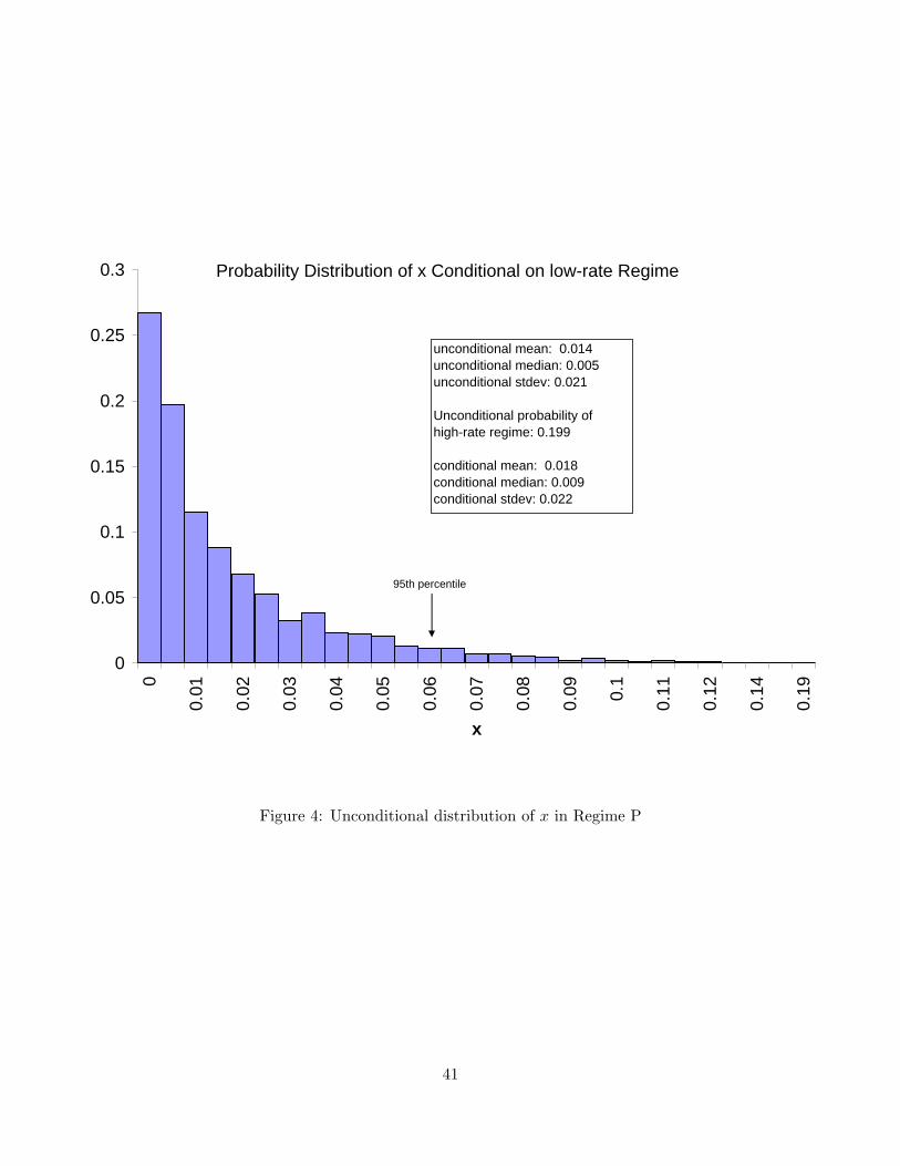
ratio). We begin by calculating the unconditional probability distribution of x in Regime P (see

Figure 4). This is done by simulating 2500 paths for xt, each 200 years in duration. The uncon-

ditional probability of being in Regime E is about 19.9%, consistent with the observations that

the high volatility regime is less persistent (Dai et al., 2003). Conditional on being in Regime P,

x resembles a Poisson distributed variable (the mean is close to the standard deviation and the

median is approximately ln 2 times the mean). Although the amount of invested capital is small

relative to the habit level, we will also see shortly that the rates at which capital is depleted or

replenished implies that it takes 2-3 years to completely deplete the median level of xt if st is

one standard deviation above its unconditional median. Intuitively, the ratcheting effect of habit

23

formation on relative risk aversion implies that even small changes in consumption growth have a

significant utility impact.19 Figure 5 depicts the probability of finding the economy in Regime E

given different values of st (i.e., Pr(x = 0, q = 0|s)). This also gives an indication as to how quickly

capital can become depleted; specifically, s = 0.9 roughly corresponds to three annual standard

deviations above the mean, reinforcing the intuition that capital can be depleted from its median

level within 2-3 years given a series of negative shocks to the endowment (i.e., positive shocks to st).

Figure 5 also gives an indication of the likelihood of negative risk-premium bonds: the probability

of st ∈ (0.868, s+), i.e. 9.05%, times the likelihood that Qt = 0 when st ∈ (0.868, s+), i.e., about

0.5. Thus one might expect, from this calibration, that once every 20 years, real bonds of duration

2-5 years may exhibit a negative risk premium. Figure 6 plots the distribution of x in Regime P

conditional on st.

We calculate and plot the (relative) investment policy, qt/yt = 1− gt − st, in Figure 7. As es-

tablished in Proposition 5, investment in the reversible technology decreases with the xt. Moreover,

investment decreases with the habit level. While intuitive, this is not generally true for s > s+.

However, this is not seen here since s+ is above the range of s depicted.

By solving Eqn. (6) we calculate bond prices for zero coupon bonds with maturity varying

from 1 to 20 years. Figure 9 depicts an estimate of the unconditional term structure, based on

the simulated distribution of (xt, st), as well as the term structures conditional on each of the two

regimes. The plots are within statistical tolerance of those estimated in Ang and Bekaert (2004).

The unconditional term structure is nearly flat, while the Regime P unconditional term structure

is slightly upward sloping and the Regime E curve steeper.

The next three figures plot the term structure of real interest rates for various values of x and

for s roughly equal to its median, as well as one unconditional standard deviation above and below

the median (s = 0.78, 0.82, 0.86). When the relative habit is at or below its unconditional mean,

the term structure is sloping up. When capital invested in the reversible technology is high, the

curve is flat in the short term, reflecting the low likelihood that regime change will take place in the

short term. At the median values for s and x (Figure 11) the term structure is humped, and the19Indeed, when b or σ is reduced, the investment policy tends to increase. For instance, in the case (b, β) = (1, 0.01)

both the median level of capital and the accompanying investment policy are roughly ten times higher.

24

hump grows more pronounced at lower levels of capital. When the relative habit is one standard

deviation above its unconditional mean (Figure 12) the term structure is still sloping up for Qt > 0,

but is slightly steeper, reflecting the increased likelihood of Regime E. This trend continues as s

increases. The Figure also illustrates a regime change: the slope of the term structure is negative

and the short rate is high relative to its value in Regime P. Figure 13 gives an indication of how

the risk premium affects the term structure by comparing bond yields when Qt = 0 for s = 0.85

with s = 0.88. When s = 0.85 rates are on average expected to decrease faster than when s = 0.88

(since both are above the median value of s). Moreover, the instantaneous short rate at s = 0.88

is higher than when s = 0.85. Thus, if the risk premium was zero, the yield curve at s = 0.85

would lie below that of s = 0.88. The figure therefore indicates that the risk premium for bonds

is sufficiently negative to shift the yield curve downward more than 50 basis points when s = 0.88

and Qt = 0. Negative bond premia can thus significantly affect the term structure despite occuring

only about 5% of the time.

We also calculate the slope of the term structure as the difference between the 20- and 1-year

yields. This is plotted in Figure 8 for both cases. Most of the variation in the slope is at low xt and

high st. We will soon show that the consumption drift is monotonically increasing in st. Thus the

slope of the term structure will forecast high growth in as much as it is negatively related to st. Since

at low st the slope is uniformly high while this is only sometimes true at high st, there is a negative

relationship between the two variables; this confirms two empirical observations summarized in

Stock and Watson (2003): the slope of the term structure can forecast economic growth, but the

forecasting power varies with time. A natural question is whether there is an alternative variable

that might do a better job forecasting growth—at least in the context of our model. The most

readily observable alternative, consistent with our model, is consumption volatility and we will

shortly test its ability to forecast consumption growth.

Figure 14 plots the volatility of consumption growth relative to the endowment volatility.

Consumption volatility decreases with xt, increases with st, and is generally smoothed by the

presence of the reversible technology. The magnitude of consumption volatility is entirely dependent

on the magnitude of labor income. NIPA data indicates that consumption volatility is about 20%

smaller than that of labor income or GNP. On the other hand, our calibration is based on a measure

25

of labor income constructed in Lettau and Ludvigson (2001) which has a much higher volatility

than the data from NIPA. Consequently, our implied consumption growth volatility is also larger

than post-war data on non-durables suggests. One can in principle, however, calibrate the model to

NIPA data instead in an attempt to capture non-durable consumption growth dynamics better.20

The expected growth rate of consumption is shown in Figure 15. It appears to be negatively related

to consumption volatility and can be higher or lower than µ; there is hardly any variation with

respect to xt save for the discontinuity during a regime shift, thus any variable that can proxy

for the relative habit will be a good predictor of consumption growth. The range of variation in

both consumption volatility and drift is about 20% and is restricted by the low levels of capital

held for the purpose of modifying the endowment. In the case (b, β) = (1, 0.01), where far more

capital is typically held in the reversible technology, consumption volatility can be 40% that of

the endowment and the expected growth rate of consumption can vary between 1.5% and 4.5%.

Finally, the market price of risk, σM shown in Figure 16, resembles consumption volatility in shape.

It is largest in Regime E and is firmly within the levels required to match the observed market

Sharpe ratio.

In summary, the model appears to qualitatively and quantitatively capture the stylized facts

listed in the Introduction: (i) regime changes where one regime is less persistent, and exhibits

high mean and volatility (Regime E); (ii) the term structure is upward (downward) sloping in the

smooth (volatile) regime. The unconditional term structure is relatively flat and seems to imply an

unconditional negative risk premium for real interest rates (i.e., positive premium for bonds); and

(iii) the risk premium for bonds is time varying and can be negative. In addition, the model appears

capable of being in qualitative agreement with the observation that the slope of term structure has

limited power to forecast consumption growth.20In addition, the autocorrelation of consumption growth, as calculated from a simulation of our model, is close to

zero. While this is consistent with data from 1947-2004, it is not consistent with data from the 70’s onward. Overall,

ours does not seem to be a good model for capturing all of the peculiarities of non-durable consumption growth. On

the other hand, there are many criticisms of using the non-durable consumption time-series to explain macro-asset

pricing phenomena (see, for example, Vissing-Jørgensen (2002) and Aıt-Sahalia, Parker and Yogo (2004) among other

references).

26

4.1 Empirical Predictions

Figure 14 indicates that consumption volatility varies primarily with st. When in Regime E,

consumption volatility is near its peak and this also coincides with a high level and volatility of real

rates. The relationship is weak, however, since within each of the regimes consumption volatility

and rates are uncorrelated. Moreover, since consumption growth rates also vary primarily with st,

these should be well correlated with consumption volatility. Indeed, from Figures 14, 15 and 8 one

might expect a proxy for st, such as consumption volatility, to be a better predictor of consumption

growth than the slope of the term structure.

These observations are empirically testable and the purpose of this subsection is to examine

the degree to which they are supported by post-war U.S. data. Table I lists each data series we use

along with its source. The lower panel lists the variables constructed from the data series. Note

that we calculate four different volatility measures for consumption growth. We do this because

the volatility of this time-series appears non-stationary, decreasing by about a factor of two over

the observation period. The relative volatility estimates, σC5,ln,t and σC

5,cn,t, are meant to somewhat

account for this non-stationarity and provide a measure of the size of the standard deviation around

the observation date relative to the standard deviation over the previous 5 years. While our model

does not explicitly account for the possibility of secular trends in volatility, it is possible to do so:

the qualitative results here do not change substantively if the endowment process itself exhibits

a trend in its volatility. In particular, consumption volatility relative to that of the endowment

process (Figure 14) will look qualitatively the same. Thus the correct volatility measure in such an

economy would be the deviation from the trend, as is calculated in σC5,ln,t and σC

5,cn,t.

Table II.A presents the contemporaneous correlation between consumption volatility, real rate

levels, real rate volatility, and the probability that the smooth rate regime prevailed as estimated

by Ang and Bekaert (2004).21 Notice first that the regime probability variable has the correct

(significant) relationship with both the rate level and volatility. Moreover, the data appears to

indicate a significant positive relationship between the consumption volatility measures that are

not trend-corrected and real rate volatility. A weaker positive relationship remains after trend-21We thank Andrew Ang and Geert Bekaert for making their filtered time series of smooth regime probability

available to us.

27

correction. The table also indicates that while a significant negative relationship exists between

consumption volatility and the smooth regime likelihood (as predicted), this disappears with the

trend correction. Finally, consumption volatility does not appear to have a significant relationship

with the level of interest rates, despite the fact that the predicted relationship exists with respect

to rate volatility. Overall, the data provides support for the hypothesis that consumption volatility

exhibits a positive (though weak) correlation with the real rate level and volatility.

Table II.B presents contemporaneous correlations between the various measures in Table II.A

and the constructed habit proxy. Note that the relationship between st and interest rate series is

stronger than for the consumption volatility measures and consistent with the model predictions.

The lack of correlation with the consumption volatility measures, on the other hand, suggests that

the latter are not good proxies for st.

Table III presents correlations between lagged predictors and realized consumption growth.

We include the nominal term spread, Lettau and Ludvigson’s (2001) estimate of the consumption-

wealth ratio (CAY), and the probability that the economy was in a smooth regime as estimated by

Ang and Bekaert (2004). The latter is related to the real term spread and thus according to Harvey

(1988) has predictive power for consumption growth. We use σC5,ln,t for consumption volatility to

make the consumption volatility proxy stationary and also include the direct proxy for st. Here

too the results are supportive of the model in the sense that the trend corrected volatility measure

and the habit proxy appear to have forecasting power for consumption growth. The lower portion

of Table III reports the results of regressions that further lend support to the proposition that

consumption volatility and/or st have forecasting power for growth beyond that present in the

slope of the term structure. This finding may be particularly useful since, according to Stock and

Watson (2003), there are very few good predictors of growth.

5 Concluding Remarks

The regimes discussed here and in the literature have roughly the same duration as business cy-

cles. As briefly noted in the empirical section above, the data does appear to indicate secular

changes to the level of real rates and consumption volatility that are not entirely consistent with

28

a steady state stationary equilibrium. Our model is too simple to handle such complications, and

it seems worthwhile to study a similar problem involving multiple technological sectors so as to

introduce more than a single time scale. Related to that, a more realistic approach than provided

here might explicitly model the irreversibility of capital investment along with time variation in

production efficiency. This could be modeled, for instance, by allowing for the possibility that

existing industries receive ‘shocks’ rendering them obsolete or less efficient as other technologies

enter. Non-trivial adjustment costs and the irreversibility of investment might lead to regimes in

economy-wide investment and, possibly, tighter empirical predictions.

29

Appendix A Proofs

Proof of Theorem 1:

Let ω ∈ Ω be a generic element in Ω describing the state of the world. Define

H(y, Q, z) = q ∈ R : −Q ≤ q ≤ y − z (7)

H(ω) = (q0, q1, . . .) : qn ∈ H(yn, Qn, zn)(ω). (8)

We can now rephrase the problem as supq∈H U(q). In particular, we are interested in arg maxq∈H U(q).

Clearly H is compact. Tychonoff’s Theorem implies that H is compact in the product topology. Note

moreover that H is non-empty: consider for instance the policy q ≡ (1 − ε)y − z. Since u′(x) = x−b is

continuous, one can always find a topology-preserving metric that can be used to establish that U is upper

semi-continuous on H. By the Weierstraß maximum theorem U attains its maximum on H (see for instance

Luenberger, 1969).

Proof of Proposition 2:

Note that due to the Inada condition satisfied by u(x) we can ignore the possibility that qt∆t = −Qt. For

any finite horizon, the result is easy to derive. Note that concavity of the value function and convexity of the

control space guarantees uniqueness of the solution for both finite and infinite horizon problems. Since U(q)

is bounded and H is compact, the optimal finite horizon solution converges to the infinite horizon solution

(by the Dominated Convergence Theorem). This is therefore also true for the sequence of Euler equations

generated by taking the limit of the finite horizon problem to an infinite horizon.

Proof of Proposition 3:

This follows from setting qt = 0 and substituting η = rEt in the Euler Equation (Proposition 2), using Ito’s

Lemma and comparing terms of order dt.

Proof of Proposition 4:

Homogeneity of q follows from the Euler equation in Proposition 2 (Alternatively, see Duffie et al., 1997).

The PDE can likewise be derived by using Ito’s Lemma and comparing terms of order dt.

30

Proof of Theorem 2:

The function V1(s) and V2(g, s) in Eqn. (5) are given by,

V1(s) =(b + 1)σ2(M − C − λ)− (A−M)(C −M − λ)

M(A−M)(C −M)− s

C −M

(1− (b + 1)σ2

A−M

)− (b + 1)σ2

(A−M)(C − λ)ΦL

(Cs−λC−λ ,−M

C

)C − λ

V2(g, s) =|Cs− λ|MC f

(|Cs− λ|−A

C

g + (b + 1)σ2

(ΦL

(Cs−λC−λ ,−A

C

)C − λ

+λ + C −A(s + 1)

A(C −A)))

where

ΦL(z, ν) =∞∑

n=0

zn

n + ν

and

f(y) = |Cs(y)− λ|−MC

(1− s(y)A−M

+(b + 1)σ2

(A−M)(C − λ)ΦL

(Cs(y)−λC−λ ,−M

C

)C − λ

+s(y)

C −M

(1− (b + 1)σ2

A−M

)− (b + 1)σ2(M − C − λ)− (A−M)(C −M − λ)

M(A−M)(C −M)

)(9)

such that s(y) solves

y = |Cs(y)− λ|−AC

1− s(y) + (b + 1)σ2

(ΦL

(Cs(y)−λC−λ ,−A

C

)C − λ

+λ + C −A(s(y) + 1)

A(C −A))

with

β + b(µ− λ) + b(α + µ− λ)s(y)

1− s(y)− b(b + 1)σ2

2(1− s(y))2≥ η (10)

(Cs− λ)(Cs(y)− λ) > 0 (11)

To prove this, note first that Eqn. (4) is a quasi-linear PDE and, using the method of characteristics,

has the general solution:

0 = F (g, s) + xs

where F (g, s) solves the following linear PDE:

1− s− g =(Ag − b + 1

2σ2 s2

1− s

)Fg + (Cs− λ)Fs −MF

where M = µ− η − σ2(b + 1). The general solution to the latter is given by

F (g, s) = − g

A−M+ |Cs− λ|M

C

∫ s

|Cw − λ|−MC

((1− w)− (b + 1)σ2

2(A−M)w2

1− w

)(Cw − λ)−1dw

+|Cs− λ|MC f(g|Cs− λ|−A

C +b + 1

2σ2

∫ s

|Cw − λ|−AC

w2

1− w(Cw − λ)−1dw

)

31

where f(·) is an arbitrary differentiable function. Note that in the region s ∈ (2 λC − 1, 1) the Lerch Phi

function, ΦL(Cs−λC−λ ,−ν), is defined and that

d

ds

|Cs− λ|−ν

[ΦL

(Cs−λC−λ ,−ν

)C − λ

+λ + C(1− ν(s + 1)

C2ν(1− ν)]

= |Cs− λ|−ν s2

1− s(Cs− λ)−1

This can be easily used to demonstrate that Eqn. (5) is the general solution to (4) in the region s ∈ (2 λC−1, 1).

It remains to establish the boundary conditions.

To see that the choice of f in Eqn. (9) satisfies the boundary conditions, note that s(y) = s when

g = 1 − s, and thus F (1 − s, s) = 0; thus as long as s satisfies rE(s) ≥ η, setting x = 0 gives g = 1 − s,

as required by the boundary conditions. One now has to establish that (i) for any g > 0 there is always a

unique solution for s(y) when

y = |Cs− λ|−AC

g +

b + 12

σ2(ΦL

(Cs−λC−λ ,−A

C

)C − λ

+λ + C −A(s + 1)

A(C −A)

)and (iii) the boundary condition, g > 0 when x = 0 and rE(s) < η is satisfied, and (iii) that the solution to

the PDE is unique.

Let s− and s+ be the roots of the equation

β + b(µ− λ) + b(α + µ− λ)s(y)

1− s(y)− b(b + 1)σ2

2(1− s(y))2= η

A necessary requirements for (i) and (ii) above is that s− and s+ are real and not equal, in which case one

can assume that s− < s+, and rE(s) > η in the interval (s−, s+). Another necessary condition is that the

range of

y(s) = |Cs− λ|−AC

1− s +

b + 12

σ2(ΦL

(Cs−λC−λ ,−A

C

)C − λ

+λ + C −A(s + 1)

A(C −A)

)for s ∈ [s−, s+] is unbounded above so that s(y) has a solution for any g > 0 in the region [s−, s+]. The

existence of real roots in the interior of (0, 1) is guaranteed by the Theorem’s hypothesis. Note that for y(s)

to be unbounded in [s−, s+], it is necessary that s− < λC < s+ otherwise y(s) is finite in [s−, s+]. Given this,

note further that

d

dsy(s) =|Cs− λ|−A

C (Cs− λ)−1(−A(1− s)− (Cs− λ) +

σ2s2

1− s

)= −|Cs− λ|−A

C (Cs− λ)−1(1− s)(rE(s)− η

)So that if s− < λ

C < s+, y(s) diverges to +∞ as s → λC , and a solution to s(y) exists for any g ≥ 0. To prove

uniqueness, note that ddsy(s) is monotonic and thus invertible in each of the regions (s−, λ

C ) and ( λC , s+).

Thus the solution for s(y) satisfying the constraints in (10) and (11) is unique.

To show that the solution satisfies the boundary conditions at x →∞, first note that g can only satisfy

Eqn. (5) for arbitrary s as x →∞ if g also approaches infinity. In particular, this requires that s(y)g→∞−→ λ

C .

32

We calculate that

gx =A−M

1− |Cs(y)−λCs−λ |(A−M)/C

(12)

thus as x →∞, gx → A−M , which is our boundary condition.

Finally, we need to show that our solution is unique. To do this, it is sufficient to demonstrate that

the solution satisfies a pair of boundary condition in a closed and connected region. In particular, we must

extend the current boundary condition at x = 0 and s ∈ [s−, s+] so that it bounds some closed and connected

region. To establish this note that y(s) is decreasing in [0, s−) and increasing in [s+, 1), thus in these regions

g(0, s) exists and is greater than 1− s; moreover, for any s one can find a unique and finite x∗(s) ≥ 0 such

that g = 1− s satisfies Eqn. (5) (x∗(s) = 0 by construction when s ∈ [s−, s+]). Thus the solution specified

in Eqn. (5) and its extension to all of s ∈ [0, 1− ε] satisfies the boundary condition g = 1− s at x∗(s) and

g = (A−M)x at x = ∞, and is therefore unique.

Proof of Proposition 5:

Given Eqn. (12) in the last proof, it is sufficient to prove that s(y) > s for Cs − λ < 0 and s(y) < s for

Cs− λ > 0. Consider Cs− λ < 0; since s(y) ∈ [r−, λ/C], if s < r− then we are done. If s ∈ [r−, λ/C], then

note that x = 0, the arbitrage conditions require gx > 0; thus s(y) > s for x close to 0. However, the form

of Eqn. (12) makes a sign change in gx when s is in (r−, λ/C). Thus gx > 0 for s below λ/C. A similar

argument can be applied to the complementary region.

Appendix B

In this Appendix we argue that Models 1-3 in Section 2 are not compatible with the stylized facts outlined

in the Introduction.

In Model 1, ηt is time varying while rE is constant, thus the volatile rate regime corresponds to the case

Qt > 0 or ηt > rE . Let η be the mean of ηt. If rE ≤ η then the volatile rate regime has a higher mean than

rE , consistent with the stylized facts. However, since ηt is an AR(1) process, the unconditional likelihood

that ηt > rE is greater or equal to 50% in this case; and thus the volatile regime is at least as frequent as

the smooth regime, in contradiction with the stylized facts. If, on the other hand, rE > η, then the volatile

regime has a lower mean than rE (the smooth regime mean), also contradicting the stylized facts.

In Model 2, the endowment process can be written in continuous time as dyt

yt= µtdt + σydW y

t with

33

dµt = κ(µ− µt)dt + σµdWµt . Setting zt = 0 one can derive rE

t as is done in Proposition 3 to yield

rEt = β + bµt −

b(b + 1)2

σ2y

If Qt = 0, the economy is in the smooth regime whenever η > rEt , or alternatively,

β − η

b+ µ− b + 1

2σ2

y < µ− µt (13)

The right hand side of the last inequality is a mean-zero Normal variate. Thus the smaller the left hand

side of the inequality, the larger the likelihood of a smooth regime. One can make the left hand side small

by choosing β and b appropriately. This, however, is constrained by a growth condition similar to the one

following Lemma 1, indicating that Qt/yt mean reverts only if bµ + β − η > b2

2 σ2y. Moreover, if b < 1 then

for utility to be finite one must have β > (1− b)µ.22 Assuming µ ≈ 0.025, η ≈ 0.015 and σy < 0.05 implies

that either b must be unreasonably large — thereby implying unrealistic real rate volatility or a ‘knife edge’

model with σµ σy — or the smooth regime at Qt = 0 is characterized by µ−µt > a where a is no smaller

than 0.01. For reasonable values of σµ this yields a frequency well under 50% when Qt = 0. Note that even

when Qt > 0, the agent will deplete invested capital whenever 0.01 > µ − µt (which is, again, most of the

time). This precludes the possibility that the smooth regime can be credibly calibrated to dominate roughly

80% of the time.23

Finally, Models 1-3 exhibit time varying real rates that are monotonic in their respective state vari-

ables.24 Thus bond yields will also vary monotonically with these state variables. In the case of Model 3,

this rules out a change of sign in the risk premium associated with the real rate. The same is generally true

in the case of Models 1 and 2, although one may be able to find parameters under which it is possible to

engineer the correlation between dW yt and dWµ

t or dW ηt so as to induce a sign change in the risk premium

of bond yields.

References

Abel, Andrew B., “Asset Prices under Habit Formation and Catching Up with the Joneses,” AEA Papers

and Proceedings, May 1990, 80, 38–42.

Aıt-Sahalia, Yacine, Jonathan A. Parker and Motohiro Yogo, Ravi and Hao Zhou, “Luxury

Goods and the Equity Premium,” Journal of Finance, 2004, 59, 2959–3004.22Theorem 2 assumes b > 1. This can be extended to b > 0 as long as appropriate parameter constraints are

placed.23We’ve verified this qualitative argument numerically.24While it is slightly tedious to establish this, the proof is straight forward and we leave it to the reader. Note that

in Model 3, utility is defined over yt/zt, where zt is defined as in Model 4.

34

Ang, Andrew and Geert Bekaert, “The Term Structure of Real Rates and Expected Inflation,” April

2004. Manuscript, Columbia University.

Bansal, Ravi and Hao Zhou, “Term Structure of Interest Rates with Regime Shifts,” Journal of Finance,

2002, 57 (5), 1997–2044.

Breeden, Douglas T., “An Intertemporal Asset Pricing Model with Stochastic Consumption and Invest-

ment Opportunities,” Journal of Financial Economics, 1979, 7, 265–296.

Brock, William A., “Asset Prices in a Production Economy,” in “The Economics of Information and

Uncertainty,” Chicago: University of Chicago Press, 1982, pp. 1–46.

Campbell, John Y. and John H. Cochrane, “By Force of Habit: A Consumption-based Explanation

of Aggregate Stock Market Behavior,” Journal of Political Economy, 1999, 107 (2), 205–251.

and Robert J. Shiller, “Yield Spreads and Interest Rate Movements: A Birds Eye View,” Review of

Economic Studies, 1991, 58, 495–514.

Cassasus, Jaime, Pierre Collin-Dufresne, and Bryan Routledge, “Equilibrium Commodity Prices

with Irreversible Investment and Non-linear Technologies,” April 2004.

Cecchetti, S., P. Lam, and N. Mark, “The Equity Premium and the Risk-free Rate: Matching the

Moments,” Journal of Monetary Economics, 1993, 31, 21–45.

Chapman, David A., “Habit Formation and Aggregate Consumption,” Econometrica, 1998, 66, 1223–

1230.

Constantinides, George M., “Habit Formation: A Resolution of the Equity Premium Puzzle,” Journal

of Political Economy, 1990, 98 (3), 519–543.

Cox, John C., Jonathan E. Ingersoll, Jr., and Stephen Ross Ross, “An Intertemporal General

Equilibrium Model of Asset Prices,” Econometrica, 1985, 53, 363–384.

, , and , “A Theory of the Term Structure of Interest Rates,” Econometrica, 1985, 53, 385–408.

Dai, Qiang and Kenneth J. Singleton, “Expectations Puzzles, Time-varying Risk Premia, and Affine

Models of the Term Structure,” Journal of Financial Economics, 2002, 63, 415–441.

, , and Wei Yang, “Regime Shifts in a Dynamic Term Structure Model of U.S. Treasury Bond Yields,”

October 2003. Manuscript, New York University and Stanford University.

Deaton, Angus, “Saving and Liquidity Constraints,” Econometrica, September 1991, 59 (5), 1221–1248.

35

Detemple, Jerome B. and Fernando Zapatero, “Asset Prices in an Exchange Economy with Habit

Formation,” Econometrica, November 1991, 59 (6), 1633–1657.

Duesenberry, James, Income, Saving, and the Theory of Consumer Behavior, Harvard University Press,

1952.

Duffie, Darrell, Wendell Fleming, H. Mete Soner, and Thaleia Zariphopoulou, “Hedging in

Incomplete Markets with HARA Utility,” Journal of Economic Dynamics and Control, 1997, 21, 753–782.

Dunn, Kenneth B. and Kenneth J. Singleton, “Modeling the Term Structure of Interest Rates under

Non-separable Utility and Durability of Goods,” Journal of Financial Economics, 1986, 17, 27–55.

Epstein, Larry G. and Stanley E. Zin, “Substitution, Risk Aversion and the Temporal Behavior of

Consumption and Asset Returns I: A Theoretical Framework,” Econometrica, July 1989, 57 (4), 937–969.

Evans, Martin D. D., “Real Risk, Inflation Risk, and the Term Structure,” The Economic Journal, 2003,

113, 345–389.

Garcia, R. and P. Perron, “An Analysis of the Real Interest Rate Under Regime Shifts,” Review of

Economics and Statistics, 1996, 78 (1), 111–125.

Gray, Stephen F., “Modeling the Conditional Distribution of Interest Rates as a Regime Switching

Process,” Journal of Financial Economics, September 1996, 42 (1), 27–62.

Hamilton, James D., “Rational-Expectations Econometric Analysis of Changes in Regime: An Investi-

gation of the Term Structure of Interest Rates,” Journal of Economic Dynamics and Control, 1988, 12,

385–423.

Harvey, Campbell, “The Real Term Structure and Consumption Growth,” Journal of Financial Eco-

nomics, December 1988, 22 (2), 305–333.

Kogan, Leonid, Dmitry Livdan, and Amir Yaron, “Futures Prices in a Production Economy with

Investment Constraints,” November 2003.

Landen, C., “Bond Pricing in a Hidden Markov Model of the Short Rate,” Finance and Stochastics, 2000,

4, 371–389.

Lettau, M. and S. Ludvigson, “Consumption, Aggregate Wealth and Expected Stock Returns,” Journal

of Finance , 2001, 56, 815–849.

Lucas, Robert E. Jr., “Asset Prices in an Exchange Economy,” Econometrica, November 1978, 46 (6),

1429–1445.

36

Luenberger, David G., Optimization by Vector Space Methods, New York, New York: John Wiley & Sons,

1969.

Naik, V. and M. H. Lee, “Yield Curve Dynamics with Discrete Shifts in Economic Regimes: Theory and

Estimation,” 1997. Working paper, University of British Columbia.

Pollak, Robert A., “Habit Formation and Dynamic Demand Functions,” Journal of Political Economy,

1970, 78 (4), 745–763.

Routledge, Bryan R., Duane J. Seppi, and Chester S. Spatt, “Equilibrium Forward Curves for

Commodities,” Journal of Finance, June 2000, 55 (3), 1297–1339.

Rubinstein, Mark, “The Valuation of Uncertain Income Streams and the Pricing of Options,” Bell Journal

of Economics, Autumn 1976, 7 (2), 407–425.

Ryder, Harl and Geoffrey Heal, “Optimal Growth with Intertemporally Dependent Preferences,” Review

of Economic Studies, January 1973, 40 (1), 1–33.

Stock, James H. and Mark W. Watson, “Forecasting Output and Inflation: The Role of Asset Prices,”

Journal of Economic Literature, September 2003, 61, 788–829.

Sundaresan, Suresh M., “Intertemporally Dependent Preferences and the Volatility of Consumption and

Wealth,” Review of Financial Studies, 1989, 2, 73–89.

Vissing-Jørgensen, Annette, “Limited Asset Market Participation and the Elasticity of Inter-temporal

Substitution,” Journal of Political Economy, 2002, 110, 825–853.

Wachter, Jessica A., “A Consumption-based Model of the Term Structure of Interest Rates,” July 2004.

Manuscript, University of Pennsylvania.

37

s

rE(s)

s-s50%

s+

η

E RegimeP Regime

Figure 1: ‘Regime P’ and ‘Regime E’ rates. The dashed line corresponds to the yield on the

reversible technology. The thick and thin solid curves correspond to the interest rate for the

endowment economy, rEt , with linear habit formation. The true interest rate equals rE

t only when

both Qt = 0 and rEt ≥ η (thick solid curve).

35

Figure 1: ‘Regime P’ and ‘Regime E’ rates. The dashed line corresponds to the yield on the

reversible technology. The thick and thin solid curves correspond to the interest rate for the

endowment economy, rEt , with linear habit formation. The true interest rate equals rE

t only when

both Qt = 0 and rEt ≥ η (thick solid curve).

38

s

Probability

Figure 2: Distribution Function for st.

36

Figure 2: Distribution Function for st.

39

0.78

0.8

0.82

0.84

0.86

0.88

0.0%1.0%2.0%3.0%4.0%

5.0%

-0.1-0.08-0.06-0.04

-0.02

0

0.02

0.04

0.06

0.08

0.1

Error

x

s

Figure 3: The relative magnitude of terms ignored in approximating the PDE for gt.

37

Figure 3: The relative magnitude of terms ignored in approximating the PDE for gt.

40

0

0.05

0.1

0.15

0.2

0.25

0.3

0

0.01

0.02

0.03

0.04

0.05

0.06

0.07

0.08

0.09 0.1

0.11

0.12

0.14

0.19

x

Probability Distribution of x Conditional on low-rate Regime

unconditional mean: 0.014unconditional median: 0.005unconditional stdev: 0.021

Unconditional probability of high-rate regime: 0.199

conditional mean: 0.018conditional median: 0.009conditional stdev: 0.022

95th percentile

Figure 4: Unconditional distribution of x in Regime P

38

Figure 4: Unconditional distribution of x in Regime P

41

Probability of High-rate Regime

0

0.1

0.2

0.3

0.4

0.5

0.6

0.7

0.8

0.825 0.85 0.875 0.9

s

prob

abili

ty

Figure 5: Conditional probability, Pr(x = 0, q = 0|s), of finding the economy in Regime E.

42

0

0.02

0.04

0.06

0.08

0.1

0.75 0.8

0.85

0

0.02

0.04

0.06

0.08

0.1

Conditional Distribution of x (low-rate regime)

x

s

Figure 6: Joint distribution function in Regime P.

43

0.780.81

0.84

0.87

0.0%

0.5%

1.0%

1.5%

2.0%

2.5%

3.0%

3.5%

4.0%

4.5%

5.0%

-1.4%

-1.2%

-1.0%

-0.8%

-0.6%

-0.4%

-0.2%

0.0%

0.2%

0.4%

0.6%

q/y

x

s

Figure 7: Investment Policy.

44

0.78

0.80

0.82

0.84

0.86

0.88

0.0%

1.0%

2.0%

3.0%

4.0%

5.0%

-2.0%

-1.5%

-1.0%

-0.5%

0.0%

0.5%Slope(x,s)

x s

Figure 8: The slope of the term structure (difference between the yields on a 20 and one year zero

coupon bonds.

45

0.014

0.019

0.024

0.029

0.034

0 2 4 6 8 10 12 14 16 18 20

UnconditionalE RegimeP Regime

Figure 11: The average term structure of real rates.

45

Figure 9: The average term structure of real rates.

46

0

0.002

0.004

0.006

0.008

0.01

0.012

0.014

0.016

0.018

0.02

1 3 5 7 9 11 13 15 17 19

00.0050.010.0150.02

s 0.78

Sum of Annualized rate

Time

x

Term Structure: s=0.78

Years

Figure 10: The term structure of real rates when s = 0.78 (one unconditional standard deviation

below the median value of s).

47

0

0.005

0.01

0.015

0.02

0.025

0.03

1 3 5 7 9 11 13 15 17 19

00.0050.010.0150.02

s 0.82

Sum of Annualized rate

Time

x

Term Structure: s=0.82

Years

Figure 11: The term structure of real rates when s = 0.82 (at the median value of s).

48

0

0.005

0.01

0.015

0.02

0.025

0.03

0.035

0.04

0.045

1 3 5 7 9 11 13 15 17 19

00.0050.010.0150.02

s 0.86

Sum of Annualized rate

Time

x

Term Structure: s=0.86

Years

Figure 12: The term structure of real rates when s = 0.78 (one unconditional standard deviation

above the median value of s).

49

0

0.005

0.01

0.015

0.02

0.025

0.03

0.035

0.04

1 3 5 7 9 11 13 15 17 19

0.850.88

x 0

Sum of Annualized rate

Time

s

Term Structure: x=0

Years

Figure 15: The term structure of real rates when x = 0 and s = 0.85, 0.88.

49

Figure 13: The term structure of real rates when x = 0 and s = 0.85, 0.88.

50

0.78

0.8

0.82

0.84

0.86

0.88

0.0%

1.5%

3.0%

4.5%

0.7

0.75

0.8

0.85

0.9

0.95

1

1.05

σC(x,s)/σ

x

s

Figure 14: Consumption growth volatility as a fraction of endowment volatility.

51

0.78

0.8

0.82

0.84

0.86

0.88

0.0%

1.5%

3.0%

4.5%

2.1%

2.2%

2.3%

2.4%

2.5%

2.6%

2.7%

2.8%

2.9%

µC(x,s)

x

s

Figure 15: Expected consumption growth rate.

52

0.78

0.8

0.82

0.84

0.86

0.88

0.0%1.0%2.0%3.0%4.0%

5.0%

0.3

0.4

0.5

0.6

0.7

0.8

0.9

1

σM(x,s)

x

s

Figure 16: The market price of risk (maximum instantaneous Sharpe ratio).

53

Table I

Description of data used and data series constructed.

Series Source

3-mo treasury rate (1947Q1:2004Q1) Federal Reserve Economic Data (FRED® II)

CPI (1947Q1:2004Q1) Federal Reserve Economic Data (FRED® II)

10-yr treasury yield (1947Q1 :2004Q1) Federal Reserve Economic Data (FRED® II)

Consumption (1952Q2:2002Q3) Martin Lettau’s webpage

CAY (1952Q2:2002Q3) Martin Lettau’s webpage

Labor Income Martin Lettau’s webpage

Ang-Bekaert Regime Switching Probability (1952Q3 :2002Q3) Courtesy of Andrew Ang and Geert Bekaert

Variable Description rR,t quarter-t real interest rate (nominal 3-mo treasury rate less AR(1) forecast of

increase in CPI) yt Date-t level of labor income

σr5,c,t Standard deviation of rR,t-2 , rR,t-1 , rR,t , rR,t+1 , rR,t+2

σr5,l,t Standard deviation of rR,t-5 , rR,t-4 , rR,3 , rR,t-2 , rR,t-1

dct Change in log-consumption growth from quarter t-1 to quarter t

σc5,c,t Standard deviation of dct-2 , dct-1 , dct , dct+1 , dct+2

σc5,cn,t σc

5,c,t divided by the standard deviation of dct-20 ,…, dct-1 σc

5,l,t Standard deviation of dct-5 , dct-4 , dc3 , dct-2 , dct-1 σc

5,ln,t σc5,l,t divided by the standard deviation of dct-20 ,…, dct-1

cayt date-t value of Lettau and Ludvigson’ s CAY time-series ntst Nominal term spread (10-year treasury yield minus 3-mo T-Bill rate) prbt Ang-Bekaert estimate for the probability of being in the smooth real rate

regime at quarter-t st 20-quarter exponential smoothing of yt using model parameters (α=0.2,

λ=0.185)

Table II Correlations between measures of consumption volatility and interest rate level & volatility. Also shown are correlations with the likelihood of the smooth real rate regime as estimated by Ang and Bekaert (2004) as well as correlations with the constructed habit level.

A. 1957Q3:2002Q3

rR,t σr5,l,t σr

5,c,t prbt

σc5,l,t 0.01 0.34** 0.12* -0.13*

σc5,c,t -0.05 0.13* 0.34** -0.14*

σc5,ln,t -0.06 0.18** -0.03 0.02

σc5,cn,t -0.07 -0.04 0.2** -0.02

prbt -0.49** -0.29** -0.44**

B. rR,t σr5,c,t σr

5,l,t σc5,c,t σc

5,l,t σc5,cn,t σc

5,ln,t prbt ntst cayt st 0.16* 0.25** 0.34** 0.05 0.08 0.00 0.01 0.19** 0.35** 0.53**

Table III

Correlations between consumption growth (dct) and lagged variables

1957Q3:2002Q3

ntst-j σc5,ln,t-j prbt-j cayt-j dct-j st-j

j=1 0.19** -0.12* 0.08 -0.24** 0.33** -0.27** j=4 0.22** -0.15* 0.19** -0.07 0.11 -0.09

Forecasting regressions of consumption growth (dct) 1957Q3:2002Q3. T-stats are in small fonts.

ntst-j σc5,ln,t-j prbt-j cayt-j dct-j st-j const R2

j=1 0.12 -0.002 0.001 -0.08 0.19 -0.06 0.10 0.21 3.88 -1.47 0.75 -2.85 2.47 -2.00 4.65

j=4 0.10 -0.002 0.002 -0.05 -0.01 0.07 0.05 0.10 3.15 -1.96 2.08 -1.62 -0.18 3.01 2.62