Energy and Feasibility Analysis of Gasoline Engine Start/Stop Technology Undergraduate Honors Thesis Presented in Partial Fulfillment of the Requirements for Graduation with Distinction at The Ohio State University By Luke A. DeBruin * * * * * The Ohio State University 2013 Defense Committee: Professor Marcello Canova, Research Advisor Dr. Shawn Midlam-Mohler, Capstone Advisor
Transcript
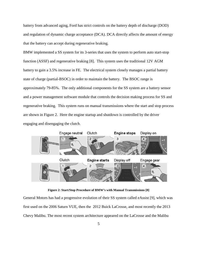
Energy and Feasibility Analysis of Gasoline Engine Start/Stop Technology
Undergraduate Honors Thesis
Presented in Partial Fulfillment of the Requirements for
Graduation with Distinction
at The Ohio State University
By
Luke A. DeBruin
* * * * *
The Ohio State University
2013
Defense Committee:
Professor Marcello Canova, Research Advisor
Dr. Shawn Midlam-Mohler, Capstone Advisor
Copyright by
Luke A. DeBruin
2013
iii
Abstract
The national mandate set forth by the Environmental Protection Agency (EPA) to increase fuel
efficiency and reduce greenhouse gas (GHG) emissions by 5% each year for all new model mid-
size cars, medium-duty cars, and light-duty trucks is pushing automobile makers to convert their
fleets to hybrid-electric and micro-hybrid vehicles. Implementing automated start/stop (SS)
technology in a passenger vehicle is a cost effective way to improve fuel economy (FE) and
reduce emissions without affecting consumer acceptance. In urban areas, where much of the
vehicle driving time is spent idling at stop lights or in traffic, the engine can be shut down when
the vehicle is stopped to save fuel. Then, the engine is quickly and quietly restarted as the driver
demands torque for acceleration. This operating strategy is often utilized in full hybrid-electric
vehicles that have powerful electric systems, but is becoming more popular in micro-hybrid
vehicles that use traditional starter/battery configurations. It is challenging to maintain
drivability and achieve efficient startups using a micro-hybrid configuration. This research
investigated the feasibility of using a micro-hybrid configuration to achieve efficient start
transients for SS technology. The energy consumption of the starter/battery was analyzed by
creating a model of the engine SS dynamics. The model was calibrated and validated through
experimental testing on a vehicle and engine that had been provided. The model was used to
simulate start transients for different component packages. Preliminary simulation results
suggest that traditional starter/battery combinations may be appropriate and a fuel savings of
over 5% may be expected in regulatory urban driving cycles. The model and selected
component package will be used for development and control of a SS system in a test vehicle.
iv
Acknowledgements
I would like to thank Dr. Giorgio Rizzoni for sparking my interest in system dynamics and for
extending the invitation to complete an honors undergraduate research project with the Center
for Automotive Research. Special thanks go to my mentor, Professor Marcello Canova, for the
time and effort he has committed to help me complete this research, and for providing to me the
diesel engine dynamics model, upon which the startup model of this research is based. I would
also like to thank research scientists Dr. Fabio Chiara and Dr. Lisa Fiorentini for their help and
support to understand the subject matter surrounding my research. Thanks to Neeraj Agarwal for
the time he spent discussing and explaining his research to me; these talks ultimately led me to
join the Chrysler Project. Ben Grimm’s analysis of start/stop using the VES provided
instrumental motivation for this work; thanks to him for the extra time he committed to produce
those results. Finally, I would like to thank graduate students Kyle Merical, Jeremy Couch,
Sandeep George, and Saba Gurusubramanian for teaching me about the engine and chassis
dynamometers and for helping me collect the experimental data used in this research.
v
Table of Contents
Page
Abstract .......................................................................................................................................... iii Acknowledgements ........................................................................................................................ iv
Table of Contents .............................................................................................................................v
List of Tables ................................................................................................................................ vii List of Figures .............................................................................................................................. viii Chapter 1: Introduction and Background ........................................................................................1
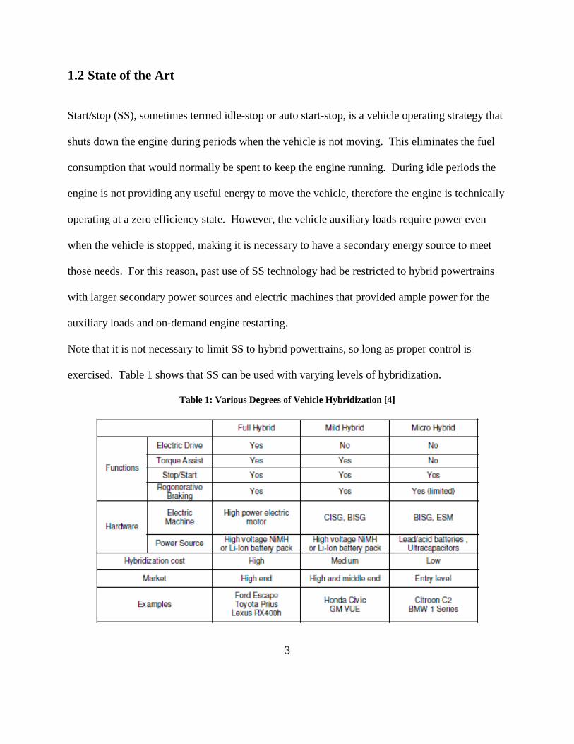
1.1 Broader Impact ...................................................................................................................1 1.2 State of the Art ....................................................................................................................3
1.2.1 Overview of Start/Stop Systems ...................................................................................4 1.2.2 Start/Stop Components..................................................................................................6 1.2.3 Start/Stop Control..........................................................................................................9
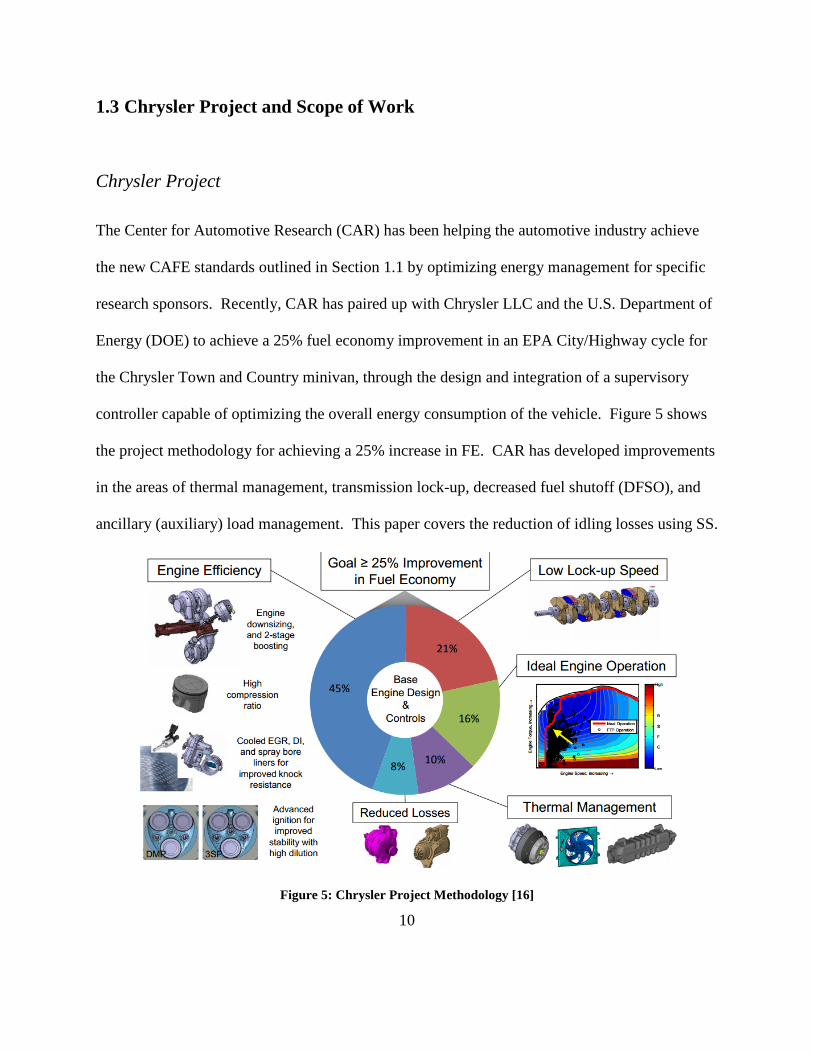
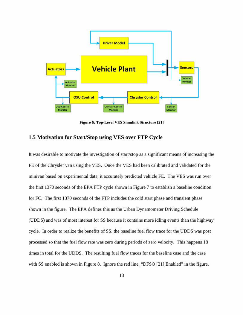
1.3 Chrysler Project and Scope of Work ................................................................................10 1.4 Vehicle Energy Simulator ................................................................................................12 1.5 Motivation for Start/Stop using VES over FTP Cycle .....................................................13 1.6 Goals, Objectives, and Fundamental Questions ...............................................................17
Chapter 2: Description of Experiments .........................................................................................18
2.3 Experimental Results ........................................................................................................27 2.3.1 Fired Engine Test Results ...........................................................................................28 2.3.2 Warm Start Test Results ..............................................................................................30 2.3.3 Isolation of Start Transient Events ..............................................................................41
Chapter 3: Model Development, Calibration and Validation ........................................................46
3.1 Model Motivation .............................................................................................................46 3.2 Model Development .........................................................................................................46
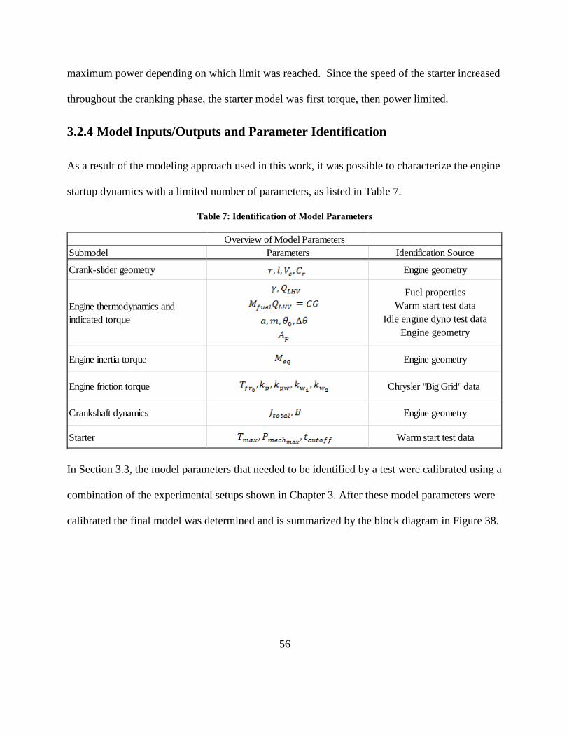
3.2.1 Engine Model ..............................................................................................................47 3.2.2 Crankshaft Model ........................................................................................................54 3.2.3 Starter Model ...............................................................................................................55 3.2.4 Model Inputs/Outputs and Parameter Identification ...................................................56
3.3 Model Calibration .............................................................................................................57 3.3.1 Engine Dynamometer Testing .....................................................................................58
vi
3.3.2 Warm Start Vehicle Tests ...........................................................................................67 3.4 Model Limitations ............................................................................................................72 3.5 Model Validation ..............................................................................................................73
Chapter 4: Energy Analyses and Start Transient Optimization .....................................................74
4.1 Overview of Analyses ......................................................................................................74 4.2 Procedure for Analyses .....................................................................................................75
4.2.1 Scaling Starter Torque .................................................................................................75 4.2.2 Combustion Gain Recalibration ..................................................................................76
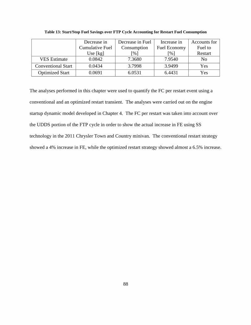
4.4 Start/Stop Fuel Economy Improvement for FTP Cycle ...................................................86
Chapter 5: Conclusion and Future Work .......................................................................................89
5.1 Summary and Conclusion .................................................................................................89 5.2 Future Work ......................................................................................................................90
5.2.1 Experimental and Modeling Refinement ....................................................................90 5.2.2 Start/Stop Component Selection and Control Development .......................................92
Figure 13: Current Shunts Installed on Electrical System [22]
23
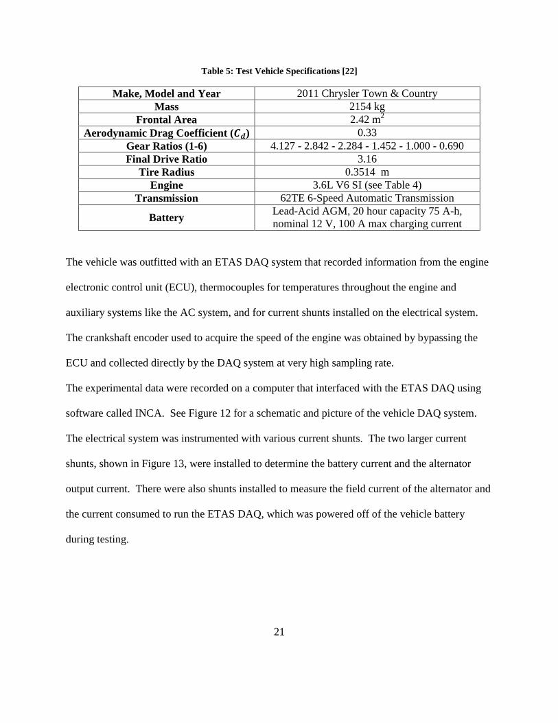
The standard procedure that the EPA uses to determine a vehicle’s published FE and emissions is
to run the vehicle over the FTP drive cycle (see Figure 7 ) on a chassis dynamometer. Because
the VES (presented in Section 1.5) was validated over the first two phases of the FTP cycle, it
was necessary to test the vehicle on CAR’s chassis dyno in order to obtain the experimental data
used for the calibration and validation of the VES. Since the VES is used to quantify FE
improvement and provide motivation for investigating SS technology, a short description of the
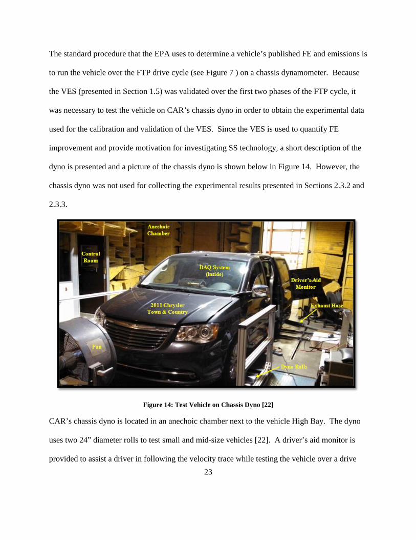
dyno is presented and a picture of the chassis dyno is shown below in Figure 14. However, the
chassis dyno was not used for collecting the experimental results presented in Sections 2.3.2 and
2.3.3.
Figure 14: Test Vehicle on Chassis Dyno [22]
CAR’s chassis dyno is located in an anechoic chamber next to the vehicle High Bay. The dyno
uses two 24” diameter rolls to test small and mid-size vehicles [22]. A driver’s aid monitor is
provided to assist a driver in following the velocity trace while testing the vehicle over a drive
24
cycle [22]. The monitor displays a LabVIEW interface that shows the upcoming velocity of the
cycle and a tolerance band to help the driver minimize the error during testing.
2.2 Experimental Methods
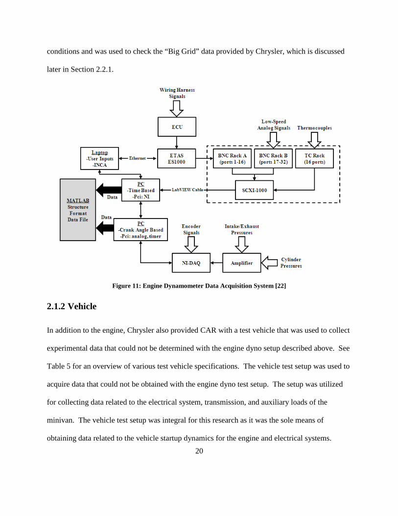
The experimental data obtained from the engine dynamometer was acquired by the DAQ system
as a low speed and a high data set and then converted with INCA software to a file format
useable in MATLAB. The low speed data set was time-based and included data from the ECU
and thermocouples. The high speed data were cycle-based and was collected as a function of
crank angle degrees (CAD). These data included intake and exhaust pressures as well as in-
cylinder pressures and encoder data. The cycle-based data were important for this work because
the model developed in Chapter 4 was crank angle resolved.
The vehicle experimental signals were post processed with MATLAB after being obtained with
the vehicle DAQ. The data set was time-based with varying sampling rates for each signal. The
crank encoder signal had the highest sampling rate in order to capture the crankshaft startup
dynamics completely. The time scales from the ECU and current shunts were scaled to match
the encoder time stamp. The signals were collected by the INCA software as .dat files and post-
processed as .mat files using a MATLAB graphical user interface (GUI).
2.2.1 Engine
One standard test that is typically conducted on engine dynamometers is to characterize the
engine performance over its entire range of operation. The operating region of the engine is
characterized by its limits for speed and torque. This test procedure is used at Chrysler and the
resulting data from this test for the 3.6L V6 was given to CAR along with the vehicle and the
25
engine. The results from this test are collected into a spreadsheet that Chrysler terms “Big Grid”
data, and it contains many engine operating parameters including temperatures, pressures, flow
rates, torques and efficiencies defined for steady-state torque and speed points. The Big Grid
data from Chrysler was checked using the engine dyno setup described above in Section 2.1.1.
The test procedure at CAR was to match and hold the engine speed at a specific Big Grid point
by setting the dyno controller to the desired engine speed. The engine torque output was set to
the target value by changing the electronic throttle position. This test procedure was used to
acquire steady-state engine data that were compared against the experimental data provided by
Chrysler. Additional tests were then conducted to characterize the engine behavior at operating
points not included in the Big Grid, specifically at low speed conditions. To this extent,
additional data were collected for three engine speeds near idle conditions at 625, 750, and 900
rpm with throttle position set as close to 0% opening as possible. The results of the low speed
tests are presented in Section 2.3.1. The data were used to calibrate the portion of the model
covered in Section 3.3.1.
2.2.2 Vehicle
The vehicle test setup was instrumental for the research described in this document.
Experimental results from the engine dyno alone do nothing to describe the startup dynamics of
the engine, which are the main interest for investigating start/stop operation. The only way to
obtain experimental results for the vehicle startup dynamics was to run tests on the vehicle in
which the start transient of the engine was captured. An initial test showed that the crankshaft
signal acquired by the ECU did not capture the area of interest for the engine startup dynamics.
In order to obtain the portion of the startup not sensed by the vehicle ECU, the crank encoder
26
signal was acquired by bypassing the ECU and collecting raw pulse data from the encoder at a
very high sampling rate. The encoder signal was later post-processed with MATLAB to obtain
the speed trace of the engine during the tests.
Start/stop technology is primarily utilized when the vehicle operating conditions are stable,
which is after the vehicle has had time to warm up and adjust to ambient conditions. Therefore,
the experimental tests were all conducted with the vehicle in the fully warmed conditions. This
was achieved by allowing the van to run for a 30 minute time frame prior to any data being
collected. After reaching stable, fully warmed conditions the vehicle was shut down for a few
minutes before the first startup test was performed.
The goal of the test procedure was to capture the start transient of the vehicle during the fully
warmed up state. First, the vehicle electronics and the DAQ system were electrified and data
collection began. Then, a key start was initiated and the resulting start transient was recorded by
the DAQ. The vehicle was left running long enough to allow the alternator to recharge the
battery. The engine idle speed was higher during the time that the battery was recharging. Once
the engine reached its lowest idle speed the van was shut down. This test was repeated three
times in succession over a 170 second time interval. The first test was 35 seconds long and tests
two and three were around 50 seconds in length each. Test one was not long enough for the
engine to reach its lowest idle speed so the time interval for the remaining tests was increased.
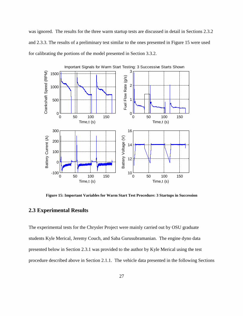
An overview of the results from the complete testing conducted on the vehicle is shown in Figure
15. The results show that test one was not long enough for the engine to reach the lowest idle
speed. The fuel flow rate between each test was zero. The data showed a constant fuel flow rate
for the time between the end of test one and the start of test two. This was a false reading and
27
was ignored. The results for the three warm startup tests are discussed in detail in Sections 2.3.2
and 2.3.3. The results of a preliminary test similar to the ones presented in Figure 15 were used
for calibrating the portions of the model presented in Section 3.3.2.
Figure 15: Important Variables for Warm Start Test Procedure: 3 Startups in Succession
2.3 Experimental Results
The experimental tests for the Chrysler Project were mainly carried out by OSU graduate
students Kyle Merical, Jeremy Couch, and Saba Gurusubramanian. The engine dyno data
presented below in Section 2.3.1 was provided to the author by Kyle Merical using the test
procedure described above in Section 2.1.1. The vehicle data presented in the following Sections
0 50 100 1500
500
1000
1500
Time,t (s)
Cra
nksh
aft S
peed
(RP
M)
Important Signals for Warm Start Testing: 3 Successive Starts Shown
0 50 100 1500
1
2
3
Time,t (s)Fu
el F
low
Rat
e (g
/s)
0 50 100 150-100
0
100
200
300
Time,t (s)
Bat
tery
Cur
rent
(A)
0 50 100 15010
12
14
16
Time,t (s)
Bat
tery
Vol
tage
(V)
28
2.3.2 and 2.3.3 was obtained by following the testing procedure detailed above in Section 2.2.2
and was carried out by Saba Gurusubramanian and the author.
2.3.1 Fired Engine Test Results
Using the engine dyno test setup described above, results for the in-cylinder pressure of cylinders
one, two, and three of the 3.6L V6 engine were obtained. Data were collected for engine
operating speeds near idle at 625, 750, and 900 rpms. The throttle was set as close to 0%
opening as possible in order to emulate the throttle position during a warm startup on the vehicle.
The engine was fired for all tests, which means that combustion occurred in the engine cylinders
during testing. More than 200 cycles of data were collected at each operating point and each of
the three cylinder pressures were synchronous averaged over this cycle interval. The results for
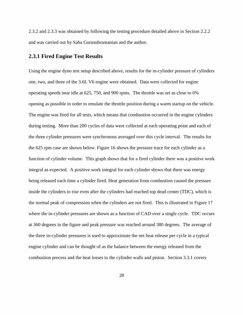
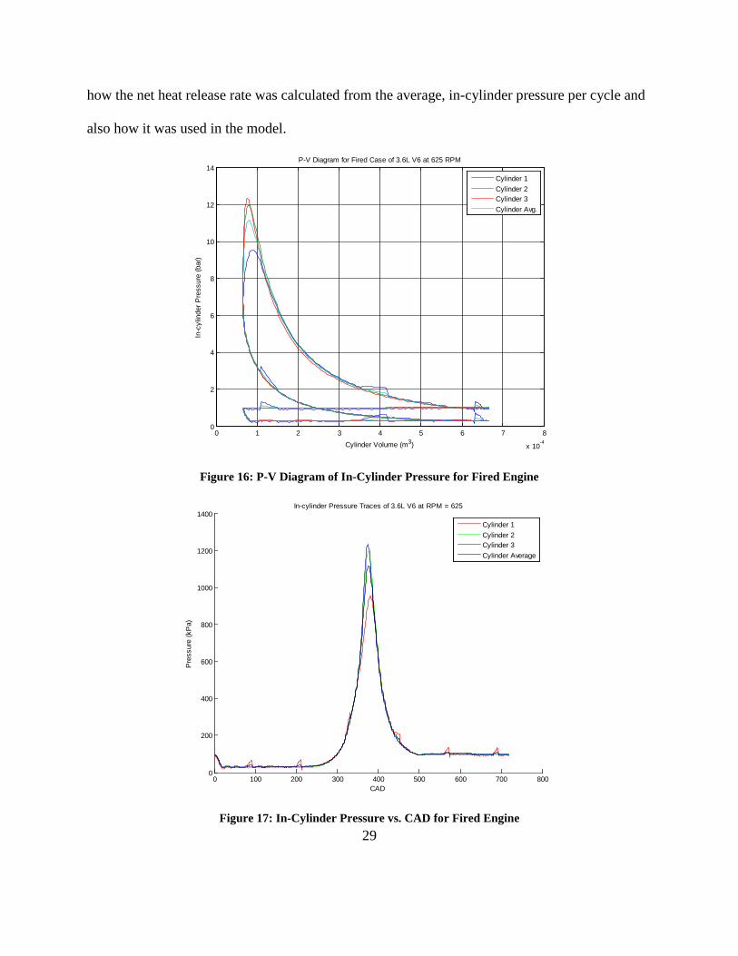
the 625 rpm case are shown below. Figure 16 shows the pressure trace for each cylinder as a
function of cylinder volume. This graph shows that for a fired cylinder there was a positive work
integral as expected. A positive work integral for each cylinder shows that there was energy
being released each time a cylinder fired. Heat generation from combustion caused the pressure
inside the cylinders to rise even after the cylinders had reached top dead center (TDC), which is
the normal peak of compression when the cylinders are not fired. This is illustrated in Figure 17
where the in-cylinder pressures are shown as a function of CAD over a single cycle. TDC occurs
at 360 degrees in the figure and peak pressure was reached around 380 degrees. The average of
the three in-cylinder pressures is used to approximate the net heat release per cycle in a typical
engine cylinder and can be thought of as the balance between the energy released from the
combustion process and the heat losses to the cylinder walls and piston. Section 3.3.1 covers
29
how the net heat release rate was calculated from the average, in-cylinder pressure per cycle and
also how it was used in the model.
Figure 16: P-V Diagram of In-Cylinder Pressure for Fired Engine
Figure 17: In-Cylinder Pressure vs. CAD for Fired Engine
0 1 2 3 4 5 6 7 8
x 10-4
0
2
4
6
8
10
12
14
Cylinder Volume (m3)
In-c
ylin
der P
ress
ure
(bar
)
P-V Diagram for Fired Case of 3.6L V6 at 625 RPM
Cylinder 1Cylinder 2Cylinder 3Cylinder Avg.
0 100 200 300 400 500 600 700 8000
200
400
600
800
1000
1200
1400In-cylinder Pressure Traces of 3.6L V6 at RPM = 625
CAD
Pre
ssur
e (k
Pa)
Cylinder 1Cylinder 2Cylinder 3Cylinder Average
30
2.3.2 Warm Start Test Results
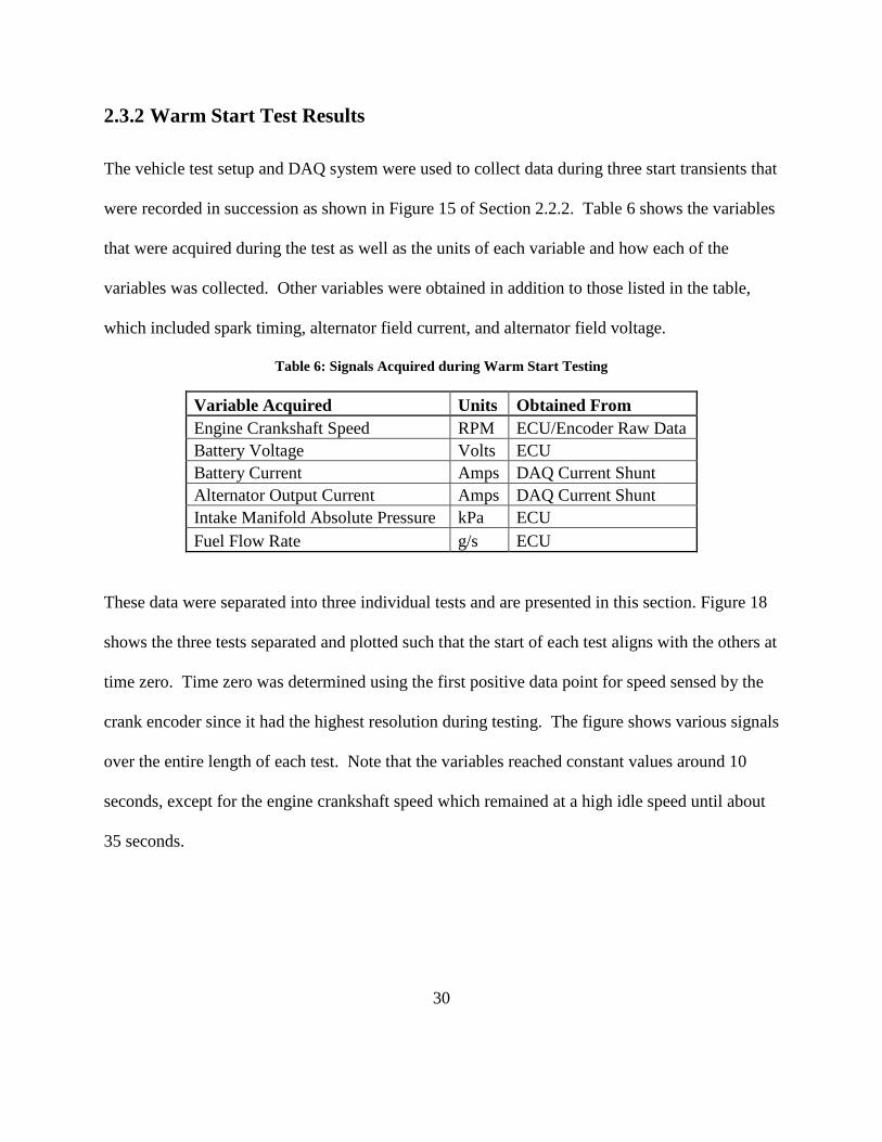
The vehicle test setup and DAQ system were used to collect data during three start transients that
were recorded in succession as shown in Figure 15 of Section 2.2.2. Table 6 shows the variables
that were acquired during the test as well as the units of each variable and how each of the
variables was collected. Other variables were obtained in addition to those listed in the table,
which included spark timing, alternator field current, and alternator field voltage.
Table 6: Signals Acquired during Warm Start Testing
Variable Acquired Units Obtained From Engine Crankshaft Speed RPM ECU/Encoder Raw Data Battery Voltage Volts ECU Battery Current Amps DAQ Current Shunt Alternator Output Current Amps DAQ Current Shunt Intake Manifold Absolute Pressure kPa ECU Fuel Flow Rate g/s ECU
These data were separated into three individual tests and are presented in this section. Figure 18
shows the three tests separated and plotted such that the start of each test aligns with the others at
time zero. Time zero was determined using the first positive data point for speed sensed by the
crank encoder since it had the highest resolution during testing. The figure shows various signals
over the entire length of each test. Note that the variables reached constant values around 10
seconds, except for the engine crankshaft speed which remained at a high idle speed until about
35 seconds.
31
Figure 18: Important Variable of Three Warm Start Tests: Full Length Tests Shown
The high idle speed of the engine was due to the idle control strategy to recharge the battery
immediately following the engine startup. The engine speed did not drop off to the normal idle
speed, which was 700 rpm, until the battery state of charge (BSOC) reached the threshold set
point. Once the battery reached the threshold BSOC the idle control commanded a linear
decrease in the speed from the higher, recharging speed to 700 rpm. In each test the start of the
linear decrease in idle speed occurred around 16 seconds. The increase in the BSOC was
observed as a hyperbolic curve in the battery current. The battery voltage was quickly
replenished and held at a constant 14 volts by the electrical system controller after the initial
voltage drop due to the energy consumed by the engine starter. This will be explained in detail
later, the point here is to note that the increase in the battery current was very small after 10
0 10 20 30 40 500
200
400
600
800
1000
1200
1400
1600
Time,t (s)
Cra
nksh
aft S
peed
(RP
M)
Important Signals from Warm Start Testing: Full Tests Shown
0 10 20 30 40 500
0.5
1
1.5
2
2.5
3x 10
-3
Time,t (s)
Fuel
Flo
w R
ate
(kg/
s)
Test 1
Test 2
Test 3
0 10 20 30 40 50-100
-50
0
50
100
150
200
250
Time,t (s)
Cur
rent
(A)
0 10 20 30 40 5010
11
12
13
14
15
Time,t (s)
Vol
tage
(V)
32
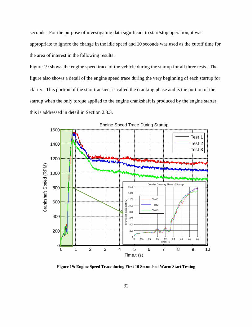
seconds. For the purpose of investigating data significant to start/stop operation, it was
appropriate to ignore the change in the idle speed and 10 seconds was used as the cutoff time for
the area of interest in the following results.
Figure 19 shows the engine speed trace of the vehicle during the startup for all three tests. The
figure also shows a detail of the engine speed trace during the very beginning of each startup for
clarity. This portion of the start transient is called the cranking phase and is the portion of the
startup when the only torque applied to the engine crankshaft is produced by the engine starter;
this is addressed in detail in Section 2.3.3.
Figure 19: Engine Speed Trace during First 10 Seconds of Warm Start Testing
0 1 2 3 4 5 6 7 8 9 100
200
400
600
800
1000
1200
1400
1600
Time,t (s)
Cra
nksh
aft S
peed
(RP
M)
Engine Speed Trace During Startup
Test 1Test 2Test 3
0 0.1 0.2 0.3 0.4 0.5 0.6 0.7 0.80
200
400
600
800
1000
1200
1400
1600
Time,t (s)
Cra
nksh
aft S
peed
(RP
M)
Detail of Cranking Phase of Startup
Test 1
Test 2
Test 3
33
Figure 19 shows that for each successive start of the vehicle, the engine crankshaft speed peak
and high idle speed decreased. For test one, the vehicle had been electrified for some time and
the vehicle auxiliary loads and the DAQ system had been draining the battery prior to the start of
test one; more so than in tests two and three, which were preceded by a reduced engine shutdown
time and hence a higher BSOC. Once the vehicle was started in test one, the vehicle idle control
commanded a high idle speed of around 1200 rpm in order to more aggressively recharge the
battery than in the other tests. In tests two and three the high idle speed was around 1100 and
1000 rpm, respectively. This successive decrease in the high idle speed commanded by the idle
controller was due to the BSOC being higher for test three than test two, and the BSOC being
higher for test two compared to test one.
Figure 20: Battery Voltage during First 10 Seconds of Warm Start Testing
0 1 2 3 4 5 6 7 8 9 1010
10.5
11
11.5
12
12.5
13
13.5
14
14.5
Time,t (s)
Vol
tage
(V)
Battery Voltage During Startup
Test 1Test 2Test 3
34
These same observations are shown by looking at the battery voltage in Figure 20. The battery
voltage showed that test one had a lower initial voltage of around 10.5 volts compared to 11.5
volts for tests two and three. Once again, the extended period of vehicle and DAQ electrification
before the start of test one accounts for the difference in initial voltage of test one compared to
tests two and three.
At the very beginning of the start transient the only torque produced to spin the crankshaft was
produced by the DC electric starter. The starter consumed energy from the battery to turn, or
crank, the engine. The energy consumed was observed in the battery voltage and current. The
initial voltage drop was due to this energy consumption. The battery voltage remained stable
after the starter stopped cranking from 0.6 to 1.14 seconds. After this point, the battery voltage
was quickly replenished. The nominal 14 volts was reached at around 4 seconds into each test.
The energy used to replenish the battery was harvested from the engine by the alternator and was
created as a direct result of the alternator field current and the high idle speed used during the
startup. This is verified by observing that the engine idle speed began to drop after 4 seconds in
Figure 19.
Figure 21 shows the battery current during the startup tests. Initially 250 amps were drawn from
the battery to supply the starter with the power to crank the engine. The current drawn dropped
to 30 amps after 0.6 seconds; this was the current necessary to power all of the vehicle ancillary
loads. At 1.14 seconds the battery current decreased linearly until reaching a lower limit of
around negative 100 amps after 4 seconds. The turn in the battery current at 4 seconds was due
to the battery reaching constant, nominal voltage. At this point the alternator duty cycle changed
35
to slowly restore the BSOC while constant battery voltage was maintained; this was observed as
a hyperbolic curve in the battery current after 4 seconds.
Figure 21: Battery Current during First 10 Seconds of Warm Start Testing
Figure 22 shows the alternator output current during the engine startup. It was observed that the
alternator began recharging the battery at 1.14 seconds and that the turn in the alternator output
current was due to the alternator controller changing the duty cycle after the battery voltage had
been restored to constant, nominal 14 volts.
0 1 2 3 4 5 6 7 8 9 10-100
-50
0
50
100
150
200
250
Time,t (s)
Cur
rent
(A)
Battery Current During Startup
Test 1Test 2Test 3
36
Figure 22: Alternator Output Current during First 10 Seconds of Warm Start Testing
The sum of the battery current and alternator output current allowed for the current drawn by the
starter and the auxiliary loads to be isolated. As noted above, the vehicle auxiliary loads drew 30
amps continuous. The sum of the currents was scaled by this 30 amp auxiliary load current.
This is referred to as the inferred starter current and is shown in Figure 23. The power consumed
by the starter during the transient was found by multiplying the inferred starter current by the
instantaneous battery voltage. The result is shown in Figure 24. Because the battery voltage
during the first 0.6 seconds of each test was constant, the electrical power consumed by the
starter was the starter current scaled by the battery voltage. This resulted in a peak power
consumption of approximately 2.5 kW when the starter was cranking.
0 1 2 3 4 5 6 7 8 9 100
50
100
150
200
Time,t (s)
Cur
rent
(A)
Alternator Output Current During Startup
Test 1Test 2Test 3
37
Figure 23: Inferred Starter Current during First 10 Seconds of Warm Start Testing
Figure 24: Inferred Starter Power during First 10 Seconds of Warm Start Testing
0 1 2 3 4 5 6 7 8 9 100
50
100
150
200
Time,t (s)
Cur
rent
(A)
Inferred Starter Current During Startup
0 0.1 0.2 0.3 0.4 0.5 0.6 0.7 0.80
50
100
150
200
Time,t (s)C
urre
nt (A
)
Detail of Inferred Starter Current
Test 1
Test 2
Test 3
0 1 2 3 4 5 6 7 8 9 100
500
1000
1500
2000
2500
Time,t (s)
Pow
er (W
)
Inferred Electrical Power Consumed by Starter During Startup
0 0.1 0.2 0.3 0.4 0.5 0.6 0.7 0.80
500
1000
1500
2000
2500
Time,t (s)
Pow
er (W
)
Detail of Inferred Electrical Power Consumed by Starter
Test 1
Test 2
Test 3
38
Figure 25 shows the torque applied to the engine crankshaft by the starter. Electrical power was
converted to mechanical power by assuming a constant motor efficiency of 90% and was
provided to the author by Chrysler. Power losses due to the gear reduction were ignored, so the
torque applied to the engine by the starter during cranking was found by dividing the starter
mechanical power by the mean angular velocity of the crankshaft during the cranking phase of
the startup. For this calculation the gear ratio between the starter pinion gear and the engine
flywheel was ignored because only the torque at the crankshaft was of interest.
Figure 25: Inferred Starter Torque at Crankshaft during First 10s of Warm Start Testing
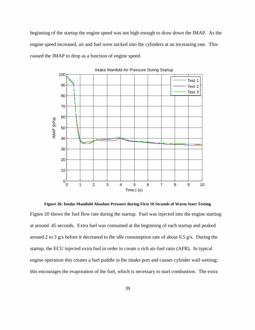
Figure 26 shows the intake manifold absolute pressure (IMAP) during the startup. Initially, the
air drawn into the engine was at the same pressure as the atmosphere, around 100 kPa. The
IMAP decreased sharply to about 40 kPa within the first second of the start transient. At the
0 1 2 3 4 5 6 7 8 9 10
0
20
40
60
80
100
120
Time,t (s)
Torq
ue (N
-m)
Inferred Starter Torque During Startup
0 0.1 0.2 0.3 0.4 0.5 0.6 0.7 0.80
20
40
60
80
100
120
Time,t (s)
Torq
ue (N
-m)
Inferred Starter Torque Detail
Test 1
Test 2
Test 3
39
beginning of the startup the engine speed was not high enough to draw down the IMAP. As the
engine speed increased, air and fuel were sucked into the cylinders at an increasing rate. This
caused the IMAP to drop as a function of engine speed.
Figure 26: Intake Manifold Absolute Pressure during First 10 Seconds of Warm Start Testing
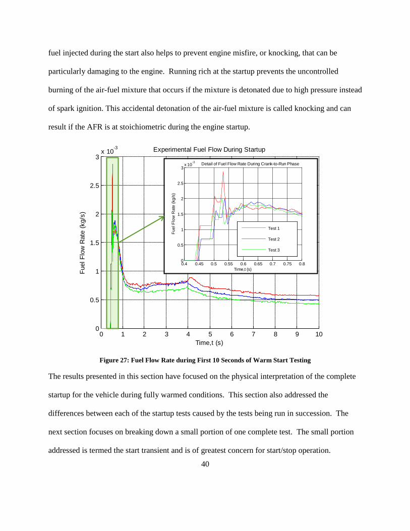
Figure 20 shows the fuel flow rate during the startup. Fuel was injected into the engine starting
at around .45 seconds. Extra fuel was consumed at the beginning of each startup and peaked
around 2 to 3 g/s before it decreased to the idle consumption rate of about 0.5 g/s. During the
startup, the ECU injected extra fuel in order to create a rich air-fuel ratio (AFR). In typical
engine operation this creates a fuel puddle in the intake port and causes cylinder wall wetting;
this encourages the evaporation of the fuel, which is necessary to start combustion. The extra
0 1 2 3 4 5 6 7 8 9 100
10
20
30
40
50
60
70
80
90
100
Time,t (s)
IMA
P (k
Pa)
Intake Manifold Air Pressure During Startup
Test 1Test 2Test 3
40
fuel injected during the start also helps to prevent engine misfire, or knocking, that can be
particularly damaging to the engine. Running rich at the startup prevents the uncontrolled
burning of the air-fuel mixture that occurs if the mixture is detonated due to high pressure instead
of spark ignition. This accidental detonation of the air-fuel mixture is called knocking and can
result if the AFR is at stoichiometric during the engine startup.
Figure 27: Fuel Flow Rate during First 10 Seconds of Warm Start Testing
The results presented in this section have focused on the physical interpretation of the complete
startup for the vehicle during fully warmed conditions. This section also addressed the
differences between each of the startup tests caused by the tests being run in succession. The
next section focuses on breaking down a small portion of one complete test. The small portion
addressed is termed the start transient and is of greatest concern for start/stop operation.
0 1 2 3 4 5 6 7 8 9 100
0.5
1
1.5
2
2.5
3x 10
-3
Time,t (s)
Fuel
Flo
w R
ate
(kg/
s)
Experimental Fuel Flow During Startup
Test 1Test 2Test 3
0.4 0.45 0.5 0.55 0.6 0.65 0.7 0.75 0.80
0.5
1
1.5
2
2.5
3x 10
-3
Time,t (s)
Fuel
Flo
w R
ate
(kg/
s)
Detail of Fuel Flow Rate During Crank-to-Run Phase
Test 1
Test 2
Test 3
41
2.3.3 Isolation of Start Transient Events
For the purpose of modeling and the analysis conducted in Chapter 5 it is necessary to define the
end of the start transient and isolate the various events that occur during this time. Figure 28
shows how the start transient is defined and broken down into separate events. Once the
alternator output current became positive in the figure it was determined that the vehicle idle
speed controller had taken over the engine dynamics. This occurred at 1.14 seconds for the
second warm startup test. After this point, the alternator was turned on and the vehicle began to
recharge the battery using the high idle speed as described in Section 2.3.2 . The engine
consumed extra fuel to produce this high idle speed. During the high idle, the extra fuel energy
was converted by the alternator into electrical energy that was stored in the battery. This energy
is not part of the start transient and must not be included when considering start/stop operation.
Therefore, the start transient ended at the moment in which the alternator started recharging the
battery; this occurred at 1.14 seconds in test two of the warm start tests. Figure 29 shows that the
end of the start transient occurred around the same time for each test conducted.
There are two phases that can be defined for the start transient: the cranking phase and the crank-
to-run phase. Each phase is distinct in that the energy consumed to start the engine comes from
different sources during the start transient. The cranking phase took the engine from rest to 200
rpm; the phase lasted around .45 seconds and the end of cranking was defined by when the
engine speed began to rapidly increase due to combustion. The energy consumed during the
cranking phase came solely from the battery. The crank-to-run phase occurred from the end of
cranking at .45 seconds to the end of the start transient at 1.14 seconds. During the crank-to-run
phase, the energy consumed to increase the engine speed came from fuel energy alone.
42
Figure 28: Isolation of Start Transient Events
Figure 29: Alternator Output Torque for All Three Warm Start Tests
0 0.2 0.4 0.6 0.8 1 1.2-1
-0.5
0
0.5
1
1.5
2
Time,t (s)
Alte
rnat
or O
utpu
t Cur
rent
[A]
Comparision of Alternator Output Current for Warmstart Tests 1-3
Warmstart Test 1Warmstart Test 2Warmstart Test 3
0 0.2 0.4 0.6 0.8 1 1.2 1.4 1.6 1.8 20
200
400
600
800
1000
1200
1400
1600
1800
2000
Time,t (s)
Mag
nitu
de o
f Sig
nals
Important Signals During Start Transient of Test 2
Encoder RPMFuel Flow Rate [mg/s]Battery Current [A]Alternator Output Current [A]
Cranking Crank-to-Run Idle Speed Control
End of Start Transient
End of Cranking
43
During the cranking phase, the DC electric starter was powered and provided a torque to the
engine crankshaft that spun it up to the cranking speed of 200 rpm. This starter torque was
determined experimentally from the variables collected during the warm start tests. Figure 30
shows the battery current and alternator output current. The superposition of these two current
signals during the start transient was equal to the starter current plus the electrified auxiliary
loads on the vehicle that were running during the start transient. From 0.6 to 1.14 seconds a 30
amp load was observed on the battery. This 30 amp load was equal to the current drawn by the
auxiliary loads because the starter only drew current from the battery from 0 to 0.6 seconds. By
scaling the superposition of the battery and alternator current the starter torque was separated
from the vehicle loads and is shown as the inferred starter current in Figure 30.
Figure 30: Current Signals for Start Transient
0 0.2 0.4 0.6 0.8 1 1.2 1.4 1.6 1.8 2
0
50
100
150
200
250
Time,t (s)
Cur
rent
(A)
Current Signals During Start Transient of Test 2
Battery Current [A]Alternator Output Current [A]Inferred Starter Current [A]
44
As mentioned above, the torque on the engine crankshaft during the cranking phase was
produced by the starter. The starter consumed battery power to provide this torque; the electrical
power consumption and the starter torque of warm start test two are shown in Figure 31 along
with intermediate data used to calculate those values. The calculation of the electrical and
mechanical power from the battery data was covered in Section 2.3.2. The figure shown here is
a synopsis of that data and is presented to show how the variables changed during the start
transient.
Figure 31: Variables Used to Calculate Starter Torque during Cranking Phase
The starter torque was found by dividing the mechanical power by the mean speed of the
crankshaft from 0.2 to 0.4 seconds of the cranking phase, which was 205 rpm. During this
portion of the cranking phase the engine speed fluctuated due to the compression events that
0 0.5 111
11.5
12
12.5
13
Time,t (s)
Bat
tery
Vol
tage
(V)
Signals of Interest for Starter Torque During the Cranking Phase
0 0.5 10
1000
2000
Time,t (s)
Sta
rter E
lect
rical
Pow
er (W
)
0 0.5 10
1000
2000
Time,t (s)
Sta
rter M
echa
nica
l Pow
er (W
)
0 0.5 10
50
100
Time,t (s)
Torq
ue (N
-m)
45
occurred in the unfired, or motored, cylinders of the engine. The pumping losses just described
can be seen in the current, power, and torque curves as sharp drops in each signal from 0.2 to 0.4
seconds.
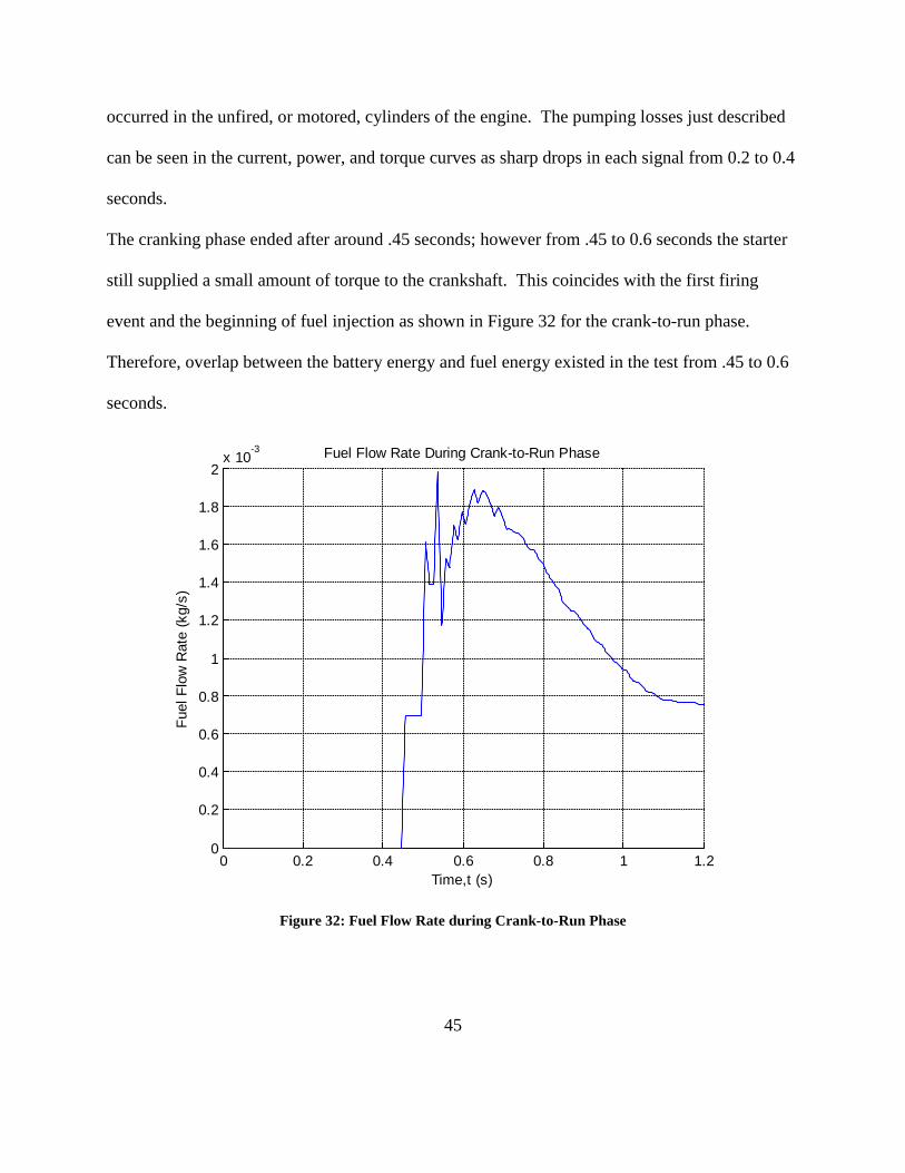
The cranking phase ended after around .45 seconds; however from .45 to 0.6 seconds the starter
still supplied a small amount of torque to the crankshaft. This coincides with the first firing
event and the beginning of fuel injection as shown in Figure 32 for the crank-to-run phase.
Therefore, overlap between the battery energy and fuel energy existed in the test from .45 to 0.6
seconds.
Figure 32: Fuel Flow Rate during Crank-to-Run Phase
0 0.2 0.4 0.6 0.8 1 1.20
0.2
0.4
0.6
0.8
1
1.2
1.4
1.6
1.8
2x 10
-3
Time,t (s)
Fuel
Flo
w R
ate
(kg/
s)
Fuel Flow Rate During Crank-to-Run Phase
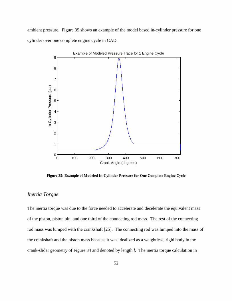
46
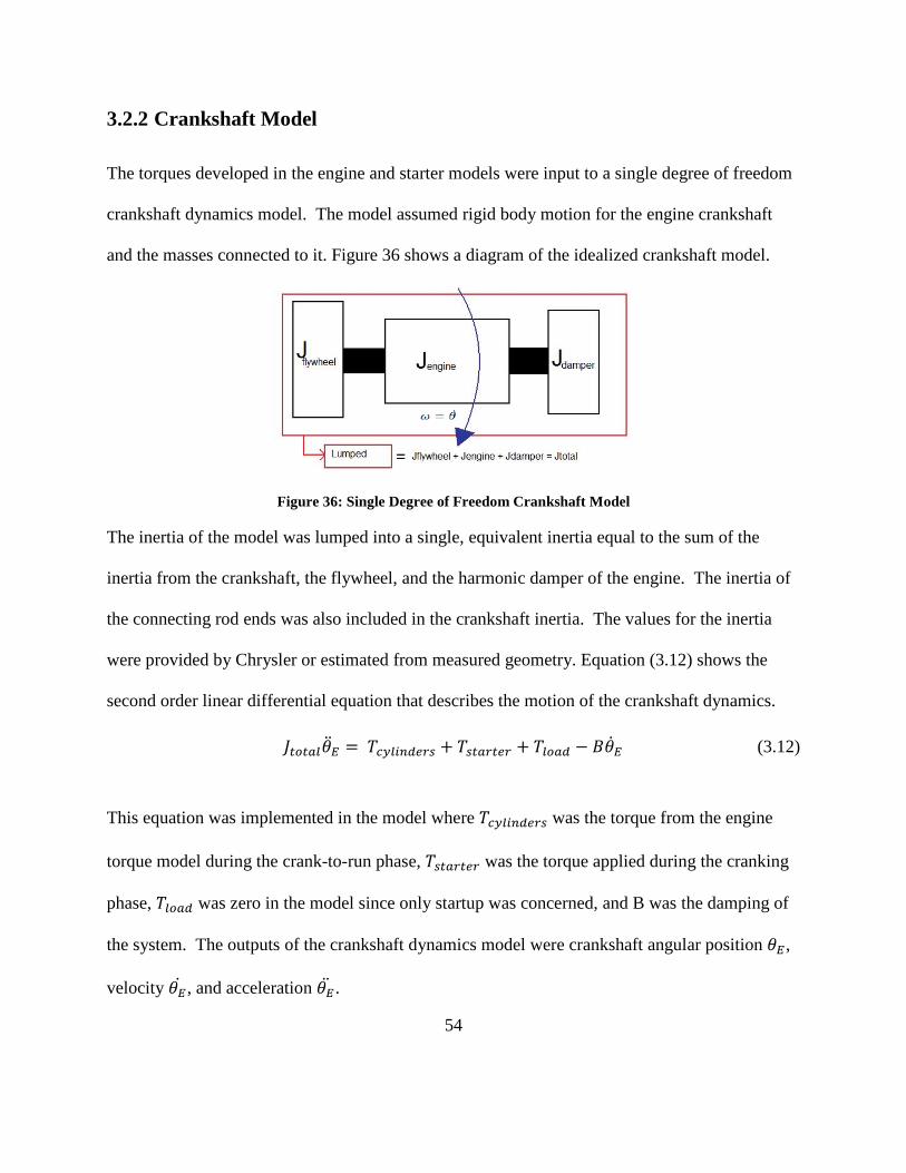
Chapter 3: Model Development, Calibration and Validation
3.1 Model Motivation
As a result of the experimental study detailed in Chapter 3, a model of the engine startup
dynamics was developed in order to further understand the relevant system dynamics and to
investigate the energy consumption from fuel and the battery during the start transient. The
model provided detailed information about the torque produced by the starter and the engine
during the start transient. This torque was input into a single degree of freedom crankshaft
model. The model was implemented in Simulink and model parameters were imported from
MATLAB. The total model is capable of accurately predicting instantaneous cylinder pressure,
torque, and engine speed. The model was calibrated and validated on preliminary experimental
results similar to the results covered in Chapter 3.
3.2 Model Development
To capture the startup dynamics during the start transient, it was necessary for the model to have
a high resolution in order to characterize the torque and speed fluctuations associated with the
engine firing events. The dynamics associated with the cranking phase were accounted for by
creating a saturation limited starter model that was input to the crankshaft model. The dynamics
related to the crank-to-run phase and idle speed conditions were accounted for by coupling a
crank angle based model of the engine torque output with the crankshaft model. Figure 33 shows
a diagram of the model hierarchy. The rest of this section describes in detail the assumptions and
the governing equations that characterize the system components of the engine startup model.
47
Figure 33: Crank Angle Based Model Hierarchy (Starter Model Not Shown)
3.2.1 Engine Model
Crank-Slider Geometry, Volume, and Brake Torque
The engine torque model characterized the instantaneous torque fluctuations of the six cylinder
engine by accounting for the in-cylinder thermodynamics, the crank-slider dynamics, and the
relationships between these subsystems. An accurate model is achieved by calculating the
instantaneous torque with a resolution of 1 CAD [17]. The engine torque model, developed in
the crank angle domain, considered the crankshaft position 𝜃𝐸 as the independent variable.
Figure 34 shows the crank-slider geometry that was used to calculate the instantaneous piston
position 𝑠, velocity �̇�, and acceleration �̈�.
48
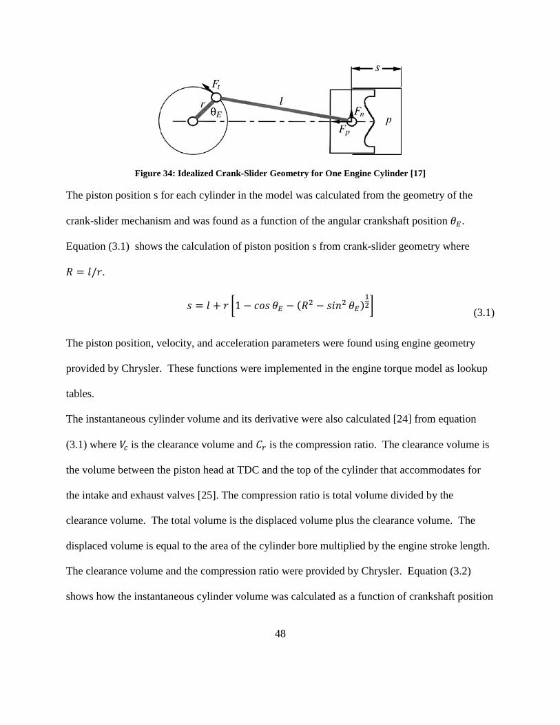
Figure 34: Idealized Crank-Slider Geometry for One Engine Cylinder [17]
The piston position s for each cylinder in the model was calculated from the geometry of the
crank-slider mechanism and was found as a function of the angular crankshaft position 𝜃𝐸 .
Equation (3.1) shows the calculation of piston position s from crank-slider geometry where
𝑅 = 𝑙/𝑟.
𝑠 = 𝑙 + 𝑟 �1 − 𝑐𝑜𝑠 𝜃𝐸 − (𝑅2 − 𝑠𝑖𝑛2 𝜃𝐸)12�
(3.1)
The piston position, velocity, and acceleration parameters were found using engine geometry
provided by Chrysler. These functions were implemented in the engine torque model as lookup
tables.
The instantaneous cylinder volume and its derivative were also calculated [24] from equation
(3.1) where 𝑉𝑐 is the clearance volume and 𝐶𝑟 is the compression ratio. The clearance volume is
the volume between the piston head at TDC and the top of the cylinder that accommodates for
the intake and exhaust valves [25]. The compression ratio is total volume divided by the
clearance volume. The total volume is the displaced volume plus the clearance volume. The
displaced volume is equal to the area of the cylinder bore multiplied by the engine stroke length.
The clearance volume and the compression ratio were provided by Chrysler. Equation (3.2)
shows how the instantaneous cylinder volume was calculated as a function of crankshaft position
49
𝜃𝐸 in the model. The volume function and its derivative were also pre-calculated in MATLAB