Energy and Charge Transfer in Open Plasmonic Systems

Energy and Charge Transfer in Open

Plasmonic Systems

Niket Thakkar

A dissertation

submitted in partial fulfillment of the

requirements for the degree of

Doctor of Philosophy

University of Washington

2017

Reading Committee:

David J. Masiello

Randall J. LeVeque

Mathew J. Lorig

Daniel R. Gamelin

Program Authorized to Offer Degree:

Applied Mathematics

©Copyright 2017

Niket Thakkar

University of Washington

Abstract

Energy and Charge Transfer in Open Plasmonic Systems

Niket Thakkar

Chair of the Supervisory Committee:

Associate Professor David J. Masiello

Chemistry

Coherent and collective charge oscillations in metal nanoparticles (MNPs), known as localized surface

plasmons, offer unprecedented control and enhancement of optical processes on the nanoscale. Since their

discovery in the 1950’s, plasmons have played an important role in understanding fundamental properties

of solid state matter and have been used for a variety of applications, from single molecule spectroscopy to

directed radiation therapy for cancer treatment. More recently, experiments have demonstrated quantum

interference between optically excited plasmonic materials, opening the door for plasmonic applications

in quantum information and making the study of the basic quantum mechanical properties of plasmonic

structures an important research topic.

This text describes a quantitatively accurate, versatile model of MNP optics that incorporates MNP

geometry, local environment, and effects due to the quantum properties of conduction electrons and radiation.

We build the theory from first principles, starting with a silver sphere in isolation and working our way

up to complex, interacting plasmonic systems with multiple MNPs and other optical resonators. We use

mathematical methods from statistical physics and quantum optics in collaboration with experimentalists to

reconcile long-standing discrepancies amongst experiments probing plasmons in the quantum size regime, to

develop and model a novel single-particle absorption spectroscopy, to predict radiative interference effects in

entangled plasmonic aggregates, and to demonstrate the existence of plasmons in photo-doped semiconductor

nanocrystals. These examples show more broadly that the theory presented is easily integrated with numerical

simulations of electromagnetic scattering and that plasmonics is an interesting test-bed for approximate

methods associated with multiscale systems.

To Mom and Dad,

for always reminding me

not to work too hard.

Contents

Acknowledgements 1

1 Introduction 3

1.1 List of Publications . . . . . . . . . . . . . . . . . . . . . . . . . . . . . . . . . . . . . . . . . . 9

2 Quantum Plasmons in Active Environments 10

2.1 Plasmon-Electon Interaction in Isolated Nanoparticles . . . . . . . . . . . . . . . . . . . . . . 11

2.2 Substrate Effects . . . . . . . . . . . . . . . . . . . . . . . . . . . . . . . . . . . . . . . . . . . 16

2.3 Active Environments . . . . . . . . . . . . . . . . . . . . . . . . . . . . . . . . . . . . . . . . . 19

2.4 Conclusion . . . . . . . . . . . . . . . . . . . . . . . . . . . . . . . . . . . . . . . . . . . . . . 21

Mathematical Complement 23

2.A Plasmons in Isolated Nanoparticles . . . . . . . . . . . . . . . . . . . . . . . . . . . . . . . . . 23

2.B Optical Properties of the Nanosphere . . . . . . . . . . . . . . . . . . . . . . . . . . . . . . . . 28

2.C LSP Decay in Free Space . . . . . . . . . . . . . . . . . . . . . . . . . . . . . . . . . . . . . . 29

2.D Substrate Effects . . . . . . . . . . . . . . . . . . . . . . . . . . . . . . . . . . . . . . . . . . . 33

2.E Finite Substrates . . . . . . . . . . . . . . . . . . . . . . . . . . . . . . . . . . . . . . . . . . . 35

2.F Hybridized Systems . . . . . . . . . . . . . . . . . . . . . . . . . . . . . . . . . . . . . . . . . 38

2.G Bulk Dielectric Properties of Silver . . . . . . . . . . . . . . . . . . . . . . . . . . . . . . . . . 42

2.H Proof of Independence of Particular and Homogenous Solutions . . . . . . . . . . . . . . . . . 44

2.I Bulk Plasmons . . . . . . . . . . . . . . . . . . . . . . . . . . . . . . . . . . . . . . . . . . . . 44

2.J Electron Energies, Wave Functions, and Shell Filling . . . . . . . . . . . . . . . . . . . . . . . 47

2.K Full wave EELS simulation . . . . . . . . . . . . . . . . . . . . . . . . . . . . . . . . . . . . . 48

2.L Data Acquisition and Analysis . . . . . . . . . . . . . . . . . . . . . . . . . . . . . . . . . . . 49

3 Optical Microresonators as Absorption Spectrometers 51

3.1 Photothermal absorption spectroscopy with sub-100-Hz detection limit . . . . . . . . . . . . . 52

3.2 Signatures of WGM-plasmon interaction . . . . . . . . . . . . . . . . . . . . . . . . . . . . . . 56

3.3 Conclusions . . . . . . . . . . . . . . . . . . . . . . . . . . . . . . . . . . . . . . . . . . . . . . 63

CONTENTS


3.A Methods . . . . . . . . . . . . . . . . . . . . . . . . . . . . . . . . . . . . . . . . . . . . . . . . 65

3.B Equations of Motion . . . . . . . . . . . . . . . . . . . . . . . . . . . . . . . . . . . . . . . . . 66

3.C Absorption and Fano Interference . . . . . . . . . . . . . . . . . . . . . . . . . . . . . . . . . . 67

3.D Extension to Many WGMs . . . . . . . . . . . . . . . . . . . . . . . . . . . . . . . . . . . . . 70

3.E Extension to 2 Nanorods . . . . . . . . . . . . . . . . . . . . . . . . . . . . . . . . . . . . . . . 71

3.F Effects of WGM Damping . . . . . . . . . . . . . . . . . . . . . . . . . . . . . . . . . . . . . . 71

3.G A Numerical Approach . . . . . . . . . . . . . . . . . . . . . . . . . . . . . . . . . . . . . . . . 72

4 Quantum Beats from Entangled Plasmons 75

4.1 Fano Resonances in the Heterodimer . . . . . . . . . . . . . . . . . . . . . . . . . . . . . . . . 76

4.2 Single Photon Dynamics and Quantum Beats . . . . . . . . . . . . . . . . . . . . . . . . . . . 81

4.3 Two-Photon Dynamics and Photon Bunching . . . . . . . . . . . . . . . . . . . . . . . . . . . 84

4.4 Conclusion . . . . . . . . . . . . . . . . . . . . . . . . . . . . . . . . . . . . . . . . . . . . . . 87


4.A Plasmon-Photon Interaction Hamiltonian . . . . . . . . . . . . . . . . . . . . . . . . . . . . . 88

5 Charge-tunable Plasmons in Semiconductor Nanocrystals 90

5.1 Results and Analysis . . . . . . . . . . . . . . . . . . . . . . . . . . . . . . . . . . . . . . . . . 91

5.2 Conclusion . . . . . . . . . . . . . . . . . . . . . . . . . . . . . . . . . . . . . . . . . . . . . . 99


5.A Methods . . . . . . . . . . . . . . . . . . . . . . . . . . . . . . . . . . . . . . . . . . . . . . . . 100

5.B Dielectric Model . . . . . . . . . . . . . . . . . . . . . . . . . . . . . . . . . . . . . . . . . . . 101

6 Concluding Remarks 104

Bibliography 105

Acknowledgements

I’d like to first and foremost thank my advisor, Professor David Masiello. David has, unsurprisingly, had a

huge influence on my research, but more than that, he was sure I’d be a successful scientist when no one,

including me, seemed to think I would be. None of this would have been possible without David’s support

and belief in my potential, and even though my qualifying exams were an incredibly stressful experience, I’ll

never forget that David is the only reason I got the opportunity to take them at all.

David’s group of misfits in the chemistry department have also been amazing to work with: Charles

Cherqui, Nick Bigelow, Steven Quillin, Nick Montoni, Jake Busche, Harrison Goldwyn, Claire West, and

Kevin Smith have all challenged me, pushed me to grow, and supported my research efforts. Charles has

had a particularly positive influence, acting as my second advisor, challenging me to make my work better,

and teaching me approaches to problem solving and mathematical modeling that I would never have learned

otherwise. Looking at his thesis, it’s pretty obvious how much influence he’s had on this one: I can’t thank

him enough for that.

I’ve had the incredible pleasure of working with a lot of experimentalists whose data is featured prominently

throughout this dissertation. Professor Daniel Gamelin and (now) Professor Alina Schimpf were my first

experimental collaborators, and I’ll always be thankful that they were willing to put up with my inexperience

in our work together. I’m also deeply grateful to Professor Randall Goldsmith and his students, Kevin

Heylman, Erik Horak, and Morgan Rea, who have been so great to work with that I’ve considered staying in

graduate school longer to continue (I won’t though).

I also want to thank my committee members: Professors Randy LeVeque, Matt Lorig, Arka Majumdar,

and Daniel Gamelin. All of them have been encouraging, happy to listen to me, and supportive of my work,

and I’m thankful to have had such diverse and discerning perspectives on my research.

I’ve had a lot of useful conversations about research that have made their way into my thesis as well.

Donsub Rim, Akash Sheth, Scott Moe, Devin Light, Dr. Robert L. Cook, Professor Hrvoje Petek, and many

others have edited my writing, talked to me about statistics or linear algebra, or listened to me complain

about all the devils in all the details that make research complicated. I’m very grateful for all of those

conversations.

Last and most importantly, I want to thank my family and friends. I’ve had endless support from my

mom, Trupti Thakkar, and my dad, Harshad Thakkar, and even though I pretend to be annoyed when they

1

2 ACKNOWLEDGEMENTS

brag about me to their friends, I’m secretly incredibly flattered. Nipa Eason, my sister, not only taught me

algebra over a summer in middle school, but also contributed significantly to the graphics throughout my

thesis - this work is as much hers as it is mine, and I would never have gotten this far without her. Nehal

Thakkar, my other sister, is easily so much smarter than me and an endless source of inspiration. When

I was 3 and she was 6, she was the one to remind me to curb my spending habits so our parents could

save for our college educations, so I suppose I have her to thank for still being trapped in school 23 years

later. Finally, I want to thank Caitlin Cornell, Ty Kunovsky, Chardon Stuart, Jeff Wheatley, and Kevin

Zimmerman for being my closest friends and strongest supports throughout the ups and downs of this entire

process. Research is difficult, and it’s people like these that make it worth all the trouble.

Chapter 1

Introduction

Understanding and controlling light has historically been a significant problem, and few technologies and

discoveries are independent of innovations in optics [1]. The study of light dates back to fifth century BC,

when Empedocles postulated that Aphrodite lit a fire within all human eyes, and that fire radiated out,

allowing humans to see. He noted that if that were true, humans could see in the night just as well as in the

day, so rays from the eyes and rays from sun must interact in some way to explain the difference [2]. Over

time, this ray representation of light gave way to particle and wave representations, all of which were finally

reconciled some 2000 years later with the discovery of quantum mechanics [3]. Along the way, studies of light

and optics have inspired the invention of a variety of technologies, from the telescope to the microscope and

beyond, all of which have pushed the limits of what the fires in people’s eyes are capable of seeing.

To that end, this text is an attempt to develop mathematical models of the electromagnetic and quantum

mechanical properties of nanoscale pieces of metal. These so-called metal nanoparticles (MNPs) support

collective and coherent oscillations of conduction electrons known as localized surface plasmons (LSPs, see Fig

1.1), which offer unprecedented control of light [4, 5], heat [6, 7], and charge [8, 9] at sub-diffraction-limited

length scales [5]. Recent advances in methods for manufacturing MNP systems of nearly arbitrary shape and

aggregation scheme have made once idealized plasmonic structures realizable, pushing the field of plasmonics

into a golden age. Since MNP aggregates offer the possibility of focusing laser light onto the nanoscale, they

represent a frontier in optics and studies of their basic properties continue to promise new applications in a

range of fields, such as biosensing [10], solar energy [11], cancer therapy [12], and selective catalysis [13].

The term surface plasmon was originally coined by Stern and Ferrell [14], but the study of plasmons dates

back to the 1950’s works of Bohm and Pines, who were able to formulate a theory describing the existence of

collective plasma oscillations in bulk metals [15, 16, 17]. Bohm and Pines showed that this collective behavior

is due to the long range part of the Coulomb interaction between conduction electrons [15, 16, 17], thereby

explaining previous experiments by Ruthemann [18] and Lang [19] on the interaction of swift electrons with

thin metal films. The theory was extended to describe surface effects by Ritchie in 1957 [20] and verified in

3

4 CHAPTER 1. INTRODUCTION

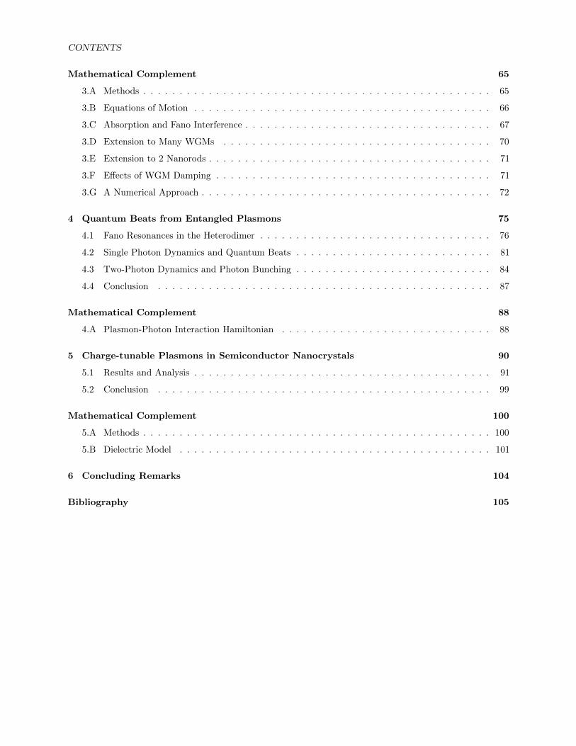
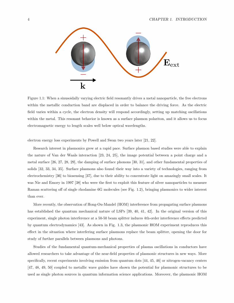
Figure 1.1: When a sinusoidally varying electric field resonantly drives a metal nanoparticle, the free electrons

within the metallic conduction band are displaced in order to balance the driving force. As the electric

field varies within a cycle, the electron density will respond accordingly, setting up matching oscillations

within the metal. This resonant behavior is known as a surface plasmon polariton, and it allows us to focus

electromagnetic energy to length scales well below optical wavelengths.

electron energy loss experiments by Powell and Swan two years later [21, 22].

Research interest in plasmonics grew at a rapid pace. Surface plasmon based studies were able to explain

the nature of Van der Waals interaction [23, 24, 25], the image potential between a point charge and a

metal surface [26, 27, 28, 29], the damping of surface phonons [30, 31], and other fundamental properties of

solids [32, 33, 34, 35]. Surface plasmons also found their way into a variety of technologies, ranging from

electrochemistry [36] to biosensing [37], due to their ability to concentrate light on amazingly small scales. It

was Nie and Emory in 1997 [38] who were the first to exploit this feature of silver nanoparticles to measure

Raman scattering off of single rhodamine 6G molecules (see Fig. 1.2), bringing plasmonics to wider interest

than ever.

More recently, the observation of Hong-Ou-Mandel (HOM) interference from propagating surface plasmons

has established the quantum mechanical nature of LSPs [39, 40, 41, 42]. In the original version of this

experiment, single photon interference at a 50-50 beam splitter induces 4th-order interference effects predicted

by quantum electrodynamics [43]. As shown in Fig. 1.3, the plasmonic HOM experiment reproduces this

effect in the situation where interfering surface plasmons replace the beam splitter, opening the door for

study of further parallels between plasmons and photons.

Studies of the fundamental quantum-mechanical properties of plasma oscillations in conductors have

allowed researchers to take advantage of the near-field properties of plasmonic structures in new ways. More

specifically, recent experiments involving emission from quantum dots [44, 45, 46] or nitrogen-vacancy centers

[47, 48, 49, 50] coupled to metallic wave guides have shown the potential for plasmonic structures to be

used as single photon sources in quantum information science applications. Moreover, the plasmonic HOM

5

Figure 1.2: Single, colloidally-formed silver MNPs are used to enhance the emission polarized Raman signal

from individual rhodamine 6G molecules. This marked the first time single molecule scattering was measured

at room temperature - a huge experimental feat, which gave rise to renewed interest in MNP optics. This

figure originally appeared in Ref. [38]

experiment shows that quantum coherences are retained in photon-plasmon-photon conversion processes

despite the significant dispersion and dephasing inherent to metallic systems [39, 40]. The possibility of

customizable, room-temperature quantum systems is significant for a variety of quantum information and

computing applications, making quantum plasmonics an exciting and growing new field [51, 52].

Studies of the quantum mechanical properties of LSPs date back to the 1960’s work of Kawabata and

Kubo [53], whose linear response theory was extended by Ganiere and coworkers [54] to predict a blueshift

in the absorption spectrum of fine spherical particles as particle size decreases and the MNP conduction

electrons’ quantum nature becomes significant. This prediction, which was in contrast to the expected result

from classical Mie theory [55], has been qualitatively verified both by modern electron energy loss experiments

[56, 57] and by a variety of theoretical approaches [58, 59, 60, 61, 62]. Still, a quantitative understanding of the

classical-to-quantum LSP transition remains elusive, and discrepancies among theoretical and experimental

approaches are not yet understood [63].

In this text, we develop a versatile, quantitatively accurate theory of MNP optics, one which can

simultaneously incorporate MNP geometry, environmental degrees of freedom such as substrates and other

optical emitters, and effects due to the quantum properties of both electrons and photons. Each chapter

below focuses on different aspects of the approach and contains work published in separate papers. Briefly:

• In chapter 2, we begin with a many-electron description of a spherical MNP, and we use a mean-field

approach to approximate the effect of Coulomb repulsion between conduction electrons. Focusing on a


Figure 1.3: Panels marked (a) correspond to the original HOM experiment while those marked (b) correspond

to the plasmonic analog. In both cases, entangled photons are generated via spontaneous parametric down

conversion and sent into a mechanism (a beam splitter in (a) and an optical fiber setup in (b)) which allows

for time delay of one beam. In (a), the indistinguishable photons interfere at the beam splitter and confirm

a prediction of quantum optics that, for short enough time delay, both photons will always take the same

path, and the two detectors will not simultaneously register a signal. In (b), interference at a beam splitter is

replaced with interference between two propagating plasmons generated with the entangled light. In both

cases, quantum electrodynamics predictions are verified, confirming the quantum nature of both light and

plasmons. These figures originally appeared in [43, 39].

7

simple system to develop our method allows us to precisely define LSPs, derive well known results in the

field, and reconcile the differences amongst experiments in the quantum plasmon regime by considering

plasmon-electron interaction in optically active environments. The material for this chapter comes from

our paper, Ref. [64].

• In chapter 3, we generalize the theory to non-spherical MNPs interacting with whispering gallery-mode

(WGM) supporting optical microresonators. This system, used by our experimental collaborators to

develop a novel single particle absorption spectroscopy, presents a difficult, multiscale mathematical

modeling problem since energy is transferred between the nanoscale LSP and the micron-scale WGMs.

We show that the theory of Chapter 2 can be used as a platform to develop multiscale numerical

methods, and we use these methods to explain Fano interference effects observed in our collaborators’

experiments. The material for this chapter comes from our paper, Ref. [65].

• In chapter 4, we incorporate plasmon-photon interaction into the theory by quantizing the electromag-

netic field, allowing us to study the quantum mechanical properties of LSP radiation. We focus on

a heterogeneous, two-sphere aggregate, and we show that this system can be thought of in terms of

analogous systems in atomic optics. Using this parallel as inspiration, we predict that properly excited

LSPs will support so-called quantum beats, interference features that have been observed in atomic

optics experiments. The material for this chapter comes from our paper, Ref. [66].

• In chapter 5, we discuss application of the theory to LSPs in doped, semiconductor nanocrystals, an

emerging new plasmonic material which supports LSPs in the infrared. Focusing on photo-doped ZnO

nanocrystals, we develop a simplified theory capable of qualitatively explaining measurements performed

by our experimental collaborators. We further comment on the application of the approach in chapter

2 to this new material, and we discuss the significance of being able to change the electron density of

plasmonic materials, a fascinating parameter that is not tunable in standard metallic systems. The

material for this chapter comes from our paper, Ref. [67].

Each chapter is split into two parts, a main body and a mathematical compliment with detailed derivations

of the theoretical results. On a first reading, the mathematical compliments can be skipped altogether and

subsequently used to answer questions and fill in details. It should be noted that this text is not a stand alone

introduction to plasmonics or nanoscale optics - that would be a much bigger undertaking. For additional

information on the topics presented, see the excellent work of Cherqui [68], Echinique [69], Novotny [70] or

Kreibig [71].

The material presented in this text also represents a step towards the development of independently

interesting mathematical methods for solving partial differential equations (PDEs) on mixed geometry,

multiscale domains. In chapter 2, we show that a conserved quantity, the Hamiltonian, can be used to

construct an approximate solution to Poisson’s equation on a domain characterized by both a spherical and a

planar interface - this is our model of a nanosphere on a substrate. Although the Laplacian is not separable


on this domain, we can solve the PDE on the sphere and plane individually, and then approximate the energy

transferred between the two pieces to construct a solution for the mixed domain. This divide and conquer

approach is not new; physicists have used similar methods on a variety of problems. Still, our generalization

to the LSP-WGM system in chapter 3 shows the flexibility offered by this viewpoint. Here, the Hamiltonian

is used to interface two numerical methods, finite elements on the micron-scale and boundary elements on

the nanoscale, effectively creating a new, multiscale numerical approach to hybrid optical systems. Although

this viewpoint on our theory is not discussed at length in the text below, it is our hope to conduct and

inspire further research on the mathematical implications and underpinnings of this general approach to

approximately solve PDEs both inside and outside nanoscale optics.

1.1. LIST OF PUBLICATIONS 9

1.1 List of Publications

This is a list of my publications in chronological order. Papers where I was lead theorist have my name in

bold.

1. Thakkar, N., Cormode, D., Lonij, V.P., Pulver, S. and Cronin, A.D., 2010, June. A simple non-linear

model for the effect of partial shade on PV systems. In Photovoltaic Specialists Conference (PVSC),

2010 35th IEEE (pp. 002321-002326). IEEE.

2. Schimpf, A.M., Thakkar, N., Gunthardt, C.E., Masiello, D.J. and Gamelin, D.R., 2013. Charge-tunable

quantum plasmons in colloidal semiconductor nanocrystals. ACS Nano, 8(1), pp.1065-1072.

3. Thakkar, N., Cherqui, C. and Masiello, D.J., 2015. Quantum beats from entangled localized surface

plasmons. ACS Photonics, 2(1), pp.157-164.

4. Wu, Y., Li, G., Cherqui, C., Bigelow, N.W., Thakkar, N., Masiello, D.J., Camden, J.P. and Rack,

P.D., 2016. Electron Energy Loss Spectroscopy Study of the Full Plasmonic Spectrum of Self-Assembled

Au–Ag Alloy Nanoparticles: Unraveling Size, Composition, and Substrate Effects. ACS Photonics, 3(1),

pp.130-138.

5. Litz, J.P., Thakkar, N., Portet, T. and Keller, S.L., 2016. Depletion with cyclodextrin reveals two

populations of cholesterol in model lipid membranes. Biophysical Journal, 110(3), pp.635-645.

6. Cherqui, C., Thakkar, N., Li, G., Camden, J.P. and Masiello, D.J., 2016. Characterizing localized

surface plasmons using electron energy-loss spectroscopy. Annual Review of Physical Chemistry, 67,

pp.331-357.

7. Cherqui, C., Wu, Y., Li, G., Quillin, S.C., Busche, J.A., Thakkar, N., West, C.A., Montoni, N.P.,

Rack, P.D., Camden, J.P. and Masiello, D.J., 2016. STEM/EELS Imaging of Magnetic Hybridization

in Symmetric and Symmetry-Broken Plasmon Oligomer Dimers and All-Magnetic Fano Interference.

Nano Letters, 16(10), pp.6668-6676.

8. Heylman, K.D., Thakkar, N., Horak, E.H., Quillin, S.C., Cherqui, C., Knapper, K.A., Masiello, D.J.

and Goldsmith, R.H., 2016. Optical microresonators as single-particle absorption spectrometers. Nature

Photonics, 10(12), pp.788-795.

9. Thakkar, N., Schimpf, A.M., Gunthardt, C.E., Gamelin, D.R. and Masiello, D.J., 2016. Comment on

“HgS and HgS/CdS Colloidal Quantum Dots with Infrared Intraband Transitions and Emergence of a

Surface Plasmon?. The Journal of Physical Chemistry C, 120(50), pp.28900-28902.

10. Thakkar, N., Montoni, N.P., Cherqui, C. and Masiello, D.J., 2017. Quantum Plasmon Resonances in

Active Environments. Nature Photonics. Under Review.

Chapter 2

Quantum Plasmons in Active

Environments

Optical manipulation of charge on the nanoscale is of fundamental importance to an array of proposed

technologies, from selective photocatalysis to nanophotonics. Open plasmonic systems, where collective

electron oscillations release energy and charge to their environments, offer a potential means to this

end as plasmons can rapidly decay into energetic electron-hole pairs; however, isolating this decay from

other plasmon-environment interactions remains a challenge. Here we present the first analytic theory

of metal nanoparticles that both quantitatively models plasmon decay into electron-hole pairs and

disentangles this effect from competing decay pathways. Using our approach, we reconcile seemingly

conflicting experiments from nanoparticle plasmonics and cluster science by accounting for substrate

effects on plasmon-electron interaction. Further examination of coupled nanoparticle-emitter systems

demonstrates that the in-phase mode more efficiently decays to photons while the out-of-phase mode

more efficiently decays to electron-hole pairs, offering a new strategy to tailor open plasmonic systems for

charge manipulation.

Localized surface plasmon (LSP) resonances, the collective oscillations of conduction-band electrons in

metal nanoparticles (MNPs), have a fundamental role in nanoscale optics and electronics [5]. These collective

phenomena offer unique control of light [4, 5], heat [6, 7], and charge [8, 9] in nanoscale systems, and studies

of their basic properties continue to promise new applications in a range of fields, such as biosensing [10],

solar energy conversion [11], cancer therapy [12], selective catalysis [13], and quantum computing [72]. The

interconversion of LSPs to individual electronic excitations, sometimes called Landau damping [73], has

gained particular experimental interest [8, 74, 75, 76, 77], and studies report changes in LSP energy and

line width due to changes in particle environment, such as substrate or embedding material [75, 76, 77], as

potential signatures of enhanced interconversion rates. Still, disentangling enhancement of electron-hole pair

generation from other effects, such as optical energy transfer [78], presents significant experimental challenges

10

2.1. PLASMON-ELECTON INTERACTION IN ISOLATED NANOPARTICLES 11

and complicates the interpretation of results. A theory of LSP-electron interaction capable of incorporating

environmental degrees of freedom, from substrates to other optical emitters, is needed to guide experiments

and offer a platform to optimize nanoparticle systems for electron-hole pair generation.

The interconversion rate of LSPs to electron-hole pairs is known to increase with decreasing MNP size

[53, 58, 59] and is therefore most significant at length scales where classical descriptions of LSPs require

quantum-mechanical modification. More recent research on MNPs [60, 61, 62], MNP aggregates [79], and

bulk metals [80, 81, 82, 83] have confirmed this result while emphasizing the importance of an accurate

description of the conduction-band electron density of states, electron spill-out, and nonlocal dielectric effects.

Meanwhile, a large body of research has taken quantum descriptions of small metal clusters and has worked to

develop atomistic models of LSPs in larger clusters [63, 84, 85, 86, 87, 88, 89, 90, 71]. In most cases, however,

MNPs are described in isolation, and the incorporation of environmental degrees of freedom is complicated

and often computationally intractable. As a result, direct comparison with experiment, where substrates and

other environmental effects are generally present, is difficult and necessitates either shifting of the data or

undesirable parameter-tuning to adjust theoretical results.

In this chapter, we present a quantitatively accurate, analytic theory of the decay of metal LSPs to

individual electronic excitations, accounting for optically active environments and the emergence of a discrete

set of electron states as MNP size decreases. We compare the theory to two experiments: (i) the electron

energy-loss spectroscopy (EELS) [91, 92] performed by Scholl et al. [57] on silver nanospheres (radius 10

nm to ∼ 1 nm) on 3 nm carbon substrates and (ii) the photofragmentation spectroscopy [93] performed by

Tiggesbaumker et al. [94] on silver clusters (radius 0.66 nm to 0.27 nm) in vacuum. After incorporating

image effects due to the substrate, we demonstrate that the theory accurately explains the blueshift in the

LSP energy observed in both experiments over decades of cluster sizes, from ∼ 245, 000 atoms to exactly 5

atoms, reconciling experiments previously thought to disagree [63]. We conclude by generalizing the theory

to predict the quantum-corrected energies of hybrid LSP-emitter systems relevant to studies of nanoparticle

assemblies [95, 96], MNP-quantum dot systems [46, 97], and LSP-enhanced molecular spectroscopies [38, 98].

Surprisingly, we find that unlike the radiative properties of LSP-emitter systems [66], the out-of-phase

LSP-emitter mode decays to electron-hole pairs most efficiently, and we suggest future experiments to measure

and control this effect.

2.1 Plasmon-Electon Interaction in Isolated Nanoparticles

To elucidate the mechanism by which LSPs disintegrate into electron-hole pairs, we first consider an isolated

silver nanosphere. The inset of Fig. 2.1 depicts a sphere with radius a characterized by infinite frequency

dielectric response ε1 embedded in material with dielectric constant ε2. Both ε1 and the plasma frequency,

ωp, are estimated by fitting a frictionless, free-electron (Drude) model to the real part of optical frequency

dielectric data [99] for bulk silver, specifying the theory’s only fit parameters.

12 CHAPTER 2. QUANTUM PLASMONS IN ACTIVE ENVIRONMENTS

3.0 4.0Energy (eV)

Exact Ref. 18Model

Figure 2.1: Absorption spectrum of a silver nanoparticle, depicted in the inset. The nanosphere’s absorption

cross section is computed with Mie theory (red curve) and the model for a particle of radius a = 10 nm in

vacuum (ε2 = 1). The MNP’s high frequency dielectric constant, ε1, and bulk plasma frequency, ωp, are

determined by parameterizing a free electron (Drude) model with bulk silver dielectric data [99]. When

the estimates of ε1 and ωp presented in the complement are used (black dashed line), the model predicts

the peak position excellently. However, if ε1 and ωp are taken from Ref. [53], the model’s predicted LSP

resonance shifts considerably (blue dashed line). The reproduction of the free space optical properties with

our parameterization is a critical confirmation of the model’s validity. This is necessary before comparison

to experimental data at small particle sizes where LSP-electron interaction becomes significant. Without

this confirmation, ε1 and ωp are essentially free parameters and can be retuned to artificially account for

environmental effects, obscuring the comparison to data.


The MNP is modeled as a set of N interacting conduction-band electrons in this static dielectric

environment; the ith electron has velocity vi and position xi and is confined by a potential, U+(xi), modeling

the positively charged ionic background in the MNP. The Lagrangian for this system is

L =∑i

[1

2mev

2i − U+(xi)

]− 1

2

∑i,j

e2

|xi − xj |, (2.1)

where e and me are the electron charge and mass and sums on i and j are over all conduction-band electrons.

Full treatment of the Coulomb interaction is difficult, and instead, we invoke a mean-field approximation,

converting it into an interaction between an electron and the superposition of the N − 1 other electrons’

electromagnetic fields. The resulting mean-field Lagrangian is

LMF =∑i

[me

2

(vi +

e

mecA(xi)

)2

− eΦ(xi)− U+(xi)

]− e2

2mec2

∑i

A2(xi) +

∫dV

8π

[ε(x)E2 −B2

],

(2.2)

where E,B,A and Φ are the collective electric field, magnetic field, vector potential, and scalar potential

produced by the conduction-band electrons, and c is the speed of light. These collective fields satisfy Maxwell’s

equations, but here we can make the further approximation that the mean-fields everywhere respond to the

motion of an individual electron instantaneously. For nanoparticle systems this approximation is very good,

and in this limit, Maxwell’s equations reduce to the Poisson equation of electrostatics. Thus, the mean-fields

can be calculated from the Green’s function, G, satisfying −ε(x)∇2G(x, t; x′, t′) = 4πδ(x − x′)δ(t − t′),

where the source charge location, x′, satisfies |x′| = r′ < a since for each electron |〈x〉| < a, and ε(x) =

ε1Θ(a − r) + ε2Θ(r − a) where Θ is the Heaviside step function. Since the left hand side of this Poisson

equation is time independent, G(x, t; x′, t′) = G(x,x′)δ(t− t′), implying that the response of the system is

instantaneous as expected in this limit. The Green’s function can then be calculated using standard methods,

resulting in

G(x,x′) =1

ε1|x− x′|+∑`m

a3(`−m)!

ε1(`+m)!

(ε1 − ε2)(`+ 1)

ε2 + `(ε1 + ε2)

[f

(1)`m (x)Θ(a− r) + f

(2)`m (x)Θ(r − a)

]f

(1)∗`m (x′), (2.3)

where f(1)`m (x) = r`Y`m(Ω)/a`+2 and f

(2)`m (x) = a`−1Y`m(Ω)/r`+1 describe the spatial fields of each multipole

moment inside and outside the sphere respectively, and Y`m(Ω) are the spherical harmonics with angular

momentum numbers ` and m. The first term in Eq. 2.3 is associated with the potential of a charge in free

space with dielectric constant ε1, and gives rise to so-called bulk plasmons [17] which are observed in both

bulk metals and MNPs [57]. The second term is the contribution of the spherical interface at r = a, and this

gives rise to LSPs. Since the first term in Eq. 2.3 is the particular solution to the Poisson equation above

and the second term is the homogenous solution, the bulk plasmons and LSPs are linearly independent and

noninteracting. As a result, the bulk term can be safely neglected moving forward.

The Green’s function can be used to calculate the fields in Eq. 2.2 by considering a charge density ρ(x, t)

defined by the electron positions at time t. Gauge transformation to eliminate Φ in favor of a longitudinal A

results in an equivalent but considerably simplified Lagrangian. Further, in the random phase approximation,


the integrals and sums over fields in Eq. 2.2 can be evaluated analytically. The corresponding Hamiltonian is

then

Hfree =∑i

[p2i

2me+ U+(xi)

]+∑`m

(V`m

2|p`m|2 +

ω2`m

2V`m|q`m|2

)− e

2mec

∑i

[pi ·A(xi) + A(xi) · pi] , (2.4)

where q`m and p`m are generalized coordinates and momenta which characterize the projection of ρ(x, t) onto

f(1)`m (x), the `,m multipole moments’ field within the nanosphere. These projections exhibit oscillator dynamics

with frequencies defined by ω2`m = `ω2

p/(`ε1 + (`+ 1)ε2), and mode volumes V`m = [3/(`ε1 + (`+ 1)ε2)]Vs

where Vs is the volume of the sphere. These are the LSPs — a set of harmonic oscillators corresponding to

net drift in the MNP’s charge density with angular momentum numbers ` and m. They characterize the

collective motion of the electrons due to their average Coulomb interaction across the MNP. The Hamiltonian

in Eq. 2.43 also introduces the electron momenta pi which couple to the collective motion through the LSP

vector potential, and it is this interaction term that governs LSP decay into electronic excitations.

The validity of these approximations and estimates of ε1 and ωp can be assessed by comparing the model’s

prediction for the MNP absorption resonance energy with that from Mie theory [55], the exact solution to

Maxwell’s equations for a dielectric sphere. This is done in Fig. 2.1, where our predicted absorption resonance

under z-polarized, plane-wave excitation (black dotted line) is compared to the Mie solution for a silver

nanosphere (a = 10 nm) computed with the fully complex-valued bulk dielectric data [99] (red line). We see

that the predicted resonance energy agrees with the exact solution, and that the excitation source selects only

the ` = 1,m = 0 LSP mode, indicating that the MNP’s optical properties are dipole-dominated at small radii.

This confirmation lends confidence to the approximations above and the parameters we use to characterize

bulk silver.

We now quantize the Hamiltonian in Eq. 2.43 and calculate the leading order effects of the electron-

plasmon interaction perturbatively. U+(x) is modeled as an infinite spherical well, and the resulting electron

wave functions and energies are approximated with the asymptotic form of the spherical Bessel function

specified in Ref. [53]. To calculate the decay rate for LSPs to electron-hole pairs, we consider transitions

between the initial and final Fock states |ϕi〉 = |110; 0e, 0h〉 and |ϕf 〉 = |010; 1e, 1h〉 of the form |N`m;ne, nh〉

with N`m plasmons in the `,m mode, and ne (nh) electrons (holes) with quantum numbers e (h). All

omitted occupation numbers are equal to zero. The restriction to the ` = 1, m = 0 LSP is made based on

the calculation above and other studies [57, 77] which show that the dipole plasmon dominates the optical

properties at small a.

Using Fermi’s golden rule, we find the LSP decay rate to electron-hole pairs

Γfree(ω10, V10) =16e2V10

hπ4a4

1

ν3

∫ 1

x0

dx√x3(x+ ν), (2.5)

where ν = hω10/εF , εF = 5.5 eV is the Fermi-energy of silver [53], and x0 = max0, 1− ν. Since V10 ∝ a3,

Γfree ∝ 1/a demonstrating that the LSP-electron coupling becomes more signifiant as MNP size decreases,

in qualitative agreement with previous studies [53, 58, 59, 60, 61]. While not obvious, we show in the


0

2

4

6

8R

adiu

s (n

m)

Energy (eV)

Free SpaceOn CarbonRef. 40Ref. 42

10

3.2 4.2

Figure 2.2: Comparison of the predicted renormalized LSP energy and data from EELS on carbon (black

circles, 2 standard deviation error bars) [57] and photofragmentation spectroscopy in vacuum (white triangles,

1 standard deviation error bars) [94], which together span a size range from ∼ 245, 000 to 5 silver atoms.

The free space model (red curve, ε2 = ε3 = 1) quantitatively agrees with the data from [94] but generally

overestimates the energies measured in [57]. However, when the model is extended to incorporate effects of

the carbon substrate (blue curve, ε2 = 1, ε3 = 3), the predicted renormalized LSP energies agree excellently

with measurement. In this comparison, bulk losses in silver, electron spill-out, ligand effects, and nonlocal

dielectric effects are all neglected. Although these can be incorporated into the model at the expense of

added complexity, our comparison shows that LSP-electron interaction and substrate effects are much more

significant determiners of the quantum plasmon energy.


complement that Γfree increases with the embedding dielectric constant, ε2, indicating that LSP decay to

electron-hole pairs is more efficient for MNPs in high dielectric materials. This transition rate can also be

used to approximate the second-order change in LSP energy, resulting in the renormalized resonance energy

hω∗10 ≈√

(hω10 + hΓ)2 − (hΓ/2)2.

In Fig. 2.2, we compare hω∗10 (red line) to data obtained via EELS on a carbon substrate [57] and to

data obtained via photofragmentation spectroscopy in vacuum [94]. In qualitative agreement with both

experiments, hω∗10 rapidly blueshifts as particle radius decreases. However, the prediction only quantitatively

agrees with the latter data measured in vacuum while generally overestimating the energy measured on the

substrate. Although it is possible to modify ε1 and ωp to shift our estimate to lower energy, this would be at

the expense of agreement with Mie theory (Fig. 2.1, blue line) and the photofragmentation spectroscopy.

Instead, we extend the theory to include substrate effects, demonstrating that the resulting LSP energies

agree with Mie theory and both experiments [57, 94].

2.2 Substrate Effects

The ` = 1,m = 0 LSP field outside the particle, stemming from f(2)10 (x), is identical to that of a point dipole

located at the sphere’s center. This observation motivates using the method of images to account for the

substrate. A point dipole with dipole moment d located above an infinite plane with dielectric constant

ε3 induces an image dipole dI = −d(ε3 − ε2)/(ε3 + ε2), in the opposite direction for the experimentally

relevant case ε3 > ε2 [78]. Although the substrates in experiments have finite thickness, the dominant image

contribution is that of the infinite half-space, which we verify by accounting for the finite substrate in the

complement. Here, for simplicity, we model the substrate as infinite (Fig. 2.3a, inset), and we modify Eq.

2.43 to include the image dipole,

Hsub = Hfree − d10 ·EI −e

2mec

∑i

[pi ·AI(xi) + AI(xi) · pi] , (2.6)

where d10 is the LSP dipole moment and EI and AI are the image field and image vector potential. Here it

is evident that the substrate affects the MNP both through direct LSP coupling and through modification of

the vector potential within the particle.

The coupling to the LSP can be diagonalized via transformation leading to a substrate-dressed LSP

with mode volume V10 = V10 − 2g and resonance frequency defined by ω210 = ω2

10(1 − 2g/V10) where

g = πa3(ε3 − ε2)(ε1 − ε2)2/6(ε3 + ε2)(ε1 + 2ε2)2, and we have assumed d10 is parallel to the substrate.

This indicates, in agreement with other studies [77], that the LSP mode volume and resonance energy both

decrease due to electrostatic substrate effects.

The remaining interaction term modifies the perturbation theory above. The LSP decay rate can be

recalculated under the approximation that the image vector potential operator, AI(xi), can be treated

as AI(〈xi〉). This approximation is valid since statistical fluctuations of the electron position will tend to

2.2. SUBSTRATE EFFECTS 17

destructively interfere as the number of electrons increases. Carrying out the perturbation theory gives

Γsub(ω10, V10) = |1− α|2 16e2V10

hπ4a4

1

ν3

∫ 1

x0

dx√x3(x+ ν)

= |1− α|2Γfree(ω10, V10),

(2.7)

for the substrate-modified rate of LSP decay into electron-hole pairs. Here ν = hω10/εF , x0 = max0, 1− ν,

and α = (ε1 − ε2)(ε3 − ε2)/24(ε3 + ε2).

The substrate-modified LSP decay rate is compared to Γfree for varying ε3 in Fig. 2.3. Interestingly,

in contrast to the ε2 dependence of Γfree, real-valued ε3 > 1 universally suppresses decay (Fig. 2.3a) since

the image dipole’s vector potential is opposite the LSP vector potential within the particle, decreasing the

coupling to electrons. Only when the substrate’s dielectric constant is complex-valued (Fig. 2.3b), indicating

that it has intrinsic losses, can energy transfer to the substrate result in an increase above the free space LSP

line width, pushing the LSP into a regime where decay to electron-hole pairs and to near-field energy transfer

become competitive. We stress, however, that this is due to intrinsic loss in the substrate, not due to the

enhancement of electron-hole pair generation, illustrating the difficulty in disentangling these processes.

Using Eq. 2.7 we can calculate the quantum-corrected, substrate-dressed LSP energy as was done

previously. This is plotted in Fig. 2.2 (blue curve) with ε3 = 3 for carbon, and we see that the modified

resonance energies agree excellently with the EELS data [57] where the free space calculation fails. Indeed,

when we compute likelihood ratios comparing the two curves (Methods), we find the substrate model is

more strongly supported by the EELS data [57] on carbon while the free space model is more strongly

supported by the photofragmentation spectroscopy data [94]. Since the previous calculation is simply a

special case (ε3 = ε2 = 1) of Eq. 2.7, we have presented a single theory that quantitatively agrees with

classical electrodynamics (Fig. 2.1) and both experiments [57, 94] over a wide range of particle sizes. Our

theory explicitly models LSP-electron interaction and substrate effects but neglects intrinsic losses in bulk

silver [99], ligand effects, and electron spill-out, while using a local dielectric function and a relatively simple

approximation to the MNP electronic structure. This indicates that LSP-electron interaction dominates

LSP loss at these sizes and that substrate effects play a much more significant role in determining quantum

plasmon properties than previously thought [57].

Interestingly, in Fig. 2.2, the EELS data appears to shift off of the substrate-modified calculation (blue

curve) and to the free space calculation (red curve) in the region below a = 3 nm. Full-wave simulation

of Maxwell’s equations for this system explains this effect, showing that substrate-induced reductions in

LSP energy are large for a > 3 nm but vanish for smaller particles. That this feature of the data can be

qualitatively reproduced in simulations indicates that it is due to retardation and not a quantum effect.


1.0

0.8

2 4 6 8 10 12 14

a.

Line

wid

th (

eV)

Radius (nm)

0.2

0.0 2 4 6 8 10

b.

Figure 2.3: (a) Substrate-dressed LSP decay to electron-hole pairs relative to Γfree as a function of substrate

dielectric constant, ε3. The suppression of the decay rate quickly saturates as ε3 increases, indicating that

the change in optical properties from free space (ε3 = 1) to any substrate (ε3 > 1) is large compared to the

change between low and high dielectric substrates. (b) Size dependence of the substrate-modified LSP line

width accounting for LSP-electron interaction and intrinsic substrate losses. The black dashed line shows

the line width in free space (ε3 = 1), and for real valued ε3 > 1 (red curve) substrate effects suppress the

interconversion between LSPs and individual electronic excitations. If ε3 is complex valued (blue curve),

intrinsic losses within the substrate can cause an increase in line width, pushing the system into a regime

where LSP decay to electron-hole pairs and to near-field interaction compete.

2.3. ACTIVE ENVIRONMENTS 19

2.3 Active Environments

We now extend the theory to incorporate an optical emitter such as a quantum dot, fluorophore, substrate

resonance, or second MNP. For simplicity, we model the LSP-emitter system in free space although the

method above can be used to include substrate effects. Furthermore, as depicted in the inset of Fig. 2.7, we

neglect the emitter’s electronic structure and instead model it as a point dipole oscillating at frequency ωem

located a distance s from the MNP surface. The Hamiltonian of Eq. 2.43 becomes

HLSP-em = Hfree +

(Vem

2p2

em +ω2

em

2Vemq2em

)− d10 ·Eem −

e

2mec

∑i

[pi ·Aem(xi) + Aem(xi) · pi] , (2.8)

where pem and qem are the generalized emitter momentum and coordinate, and Eem and Aem are the emitter

electric field and vector potential. The mode volume, Vem, is defined in connection to the emitter dipole

moment, which is assumed to take the form dem = CVempemz, where C is a dimensionless proportionality

constant that gives the results below general applicability to a wide-class of emitters. This Hamiltonian

shows that, similar to the substrate, the emitter couples both to the LSP directly and to individual electrons

through Aem.

The direct LSP coupling can again be diagonalized through transformation. This results in two hybridized

LSP-emitter normal modes with eigenfrequencies defined by

ω2− = ω2

10 cos2 θ + ω2em sin2 θ − 2gω10ωem√

V10Vem

sin θ cos θ,

ω2+ = ω2

10 sin2 θ + ω2em cos2 θ +

2gω10ωem√V10Vem

sin θ cos θ,

(2.9)

and mode volumes

V− = V10

(ω2

10

ω2em

)cos2 θ + V10 sin2 θ − 2gω10

ωem

√V10

Vemsin θ cos θ,

V+ = Vem

(ω2

em

ω210

)cos2 θ + Vem sin2 θ +

2gωeω10

√VeV10

sin θ cos θ,

(2.10)

where tan(2θ) = 2gω10ωem/√V10Vem(ω2

em − ω210), and g = 2CV10Vem(ε1 − ε2)/

√12π(a + s)3. The angle θ

characterizes the degree of mixing between the LSP and emitter and is positive when ωem > ω10. In that

case, the − and + modes correspond to the well-known in-phase (bonding) and out-of-phase (anti-bonding)

eigenmodes of a coupled dipole system [100, 66]. At θ = 0, when ω10 and ωem are sufficiently detuned

or the separation distance s is much larger than a, the LSP and emitter are nearly uncoupled and the −

mode reduces to the LSP while the + mode reduces to the emitter. On the other hand, if ω10 and ωem are

degenerate or s is very small, θ approaches 45 and the LSP and emitter are evenly mixed.

This transformation modifies the second coupling term in Eq. 2.8, and both the in-phase and out-of-phase

modes interact with electrons differently. Calculating these interaction terms, a perturbation theory can

be carried out for each mode separately, again making the approximation that Aem(xi) ≈ Aem(〈xi〉). The


In-phase mode

Energy (eV)3.2 4.0

10

8

6

4

2

0

Rad

ius

(nm

)

Out-of-phase mode

3.55 3.85Energy (eV)

10

8

6

4

2

0

Rad

ius

(nm

)

s = 1 nm

s = 5 nm

s = 10 nms

= 1

nm

s =

5 n

ms

= 1

0 nm

Figure 2.4: Evolution of the renormalized in-phase (left) and out-of-phase (right) normal modes of the coupled

MNP-optical emitter system (inset) as a function of MNP radius a. Increasing opacity signifies decreasing

separation distance s, with s = 1, 5, and 10 nm. We see that the in-phase mode tracks the uncoupled LSP

(left, black dashed line), and is shifted to lower energy as the MNP and emitter are brought together and

interact more strongly. On the other hand, the out-of-phase mode tracks the uncoupled emitter (right, black

dashed line) and shifts to higher energy as s decreases. As the MNP radius a decreases, shifting of the LSP

energy causes a rapid decoupling of the LSP and emitter, resulting in a rapid red-shift in the out-of-phase

configuration’s energy and illustrating previously unexplored quantum effects on plasmon hybridization.

2.4. CONCLUSION 21

resulting decay rates are

Γ−(ω−, V−) =

∣∣∣∣∣ωem

ω10cos θ −

√16πVem

3V10

Ca3

(a+ s)3sin θ

∣∣∣∣∣2

Γfree(ω−, V−)

Γ+(ω+, V+) =

∣∣∣∣∣√V10

Vemsin θ +

√16π

3

ω10

ωem

Ca3

(a+ s)3cos θ

∣∣∣∣∣2

Γfree(ω+, V+).

(2.11)

Notice that the emitter vector potential destructively interferes with the decay in the in-phase configuration

where A and Aem are misaligned within the particle but constructively interferes in the out-of-phase

configuration where A and Aem are aligned within the particle. This implies that if the modes are mixed,

the out-of-phase mode more efficiently decays to individual electronic excitations than the in-phase mode.

This is in stark juxtaposition to the in-phase and out-of-phase modes’ coupling to near-field energy transfer

and far-field radiation, where the in-phase mode’s larger net dipole moment makes it the more efficiently

decaying hybrid resonance [66].

Eq. 2.11 can be used just as the decay rates previously to calculate the quantum-corrected eigenenergies,

hω∗±. For the case where the emitter is another silver nanosphere with fixed radius (4 nm, hωem = 3.55 eV),

we plot in Fig. 2.7 the eigenergies as a function of a for three separation distances, s = 1, 5, and 10 nm, and

we compare to the uncoupled (g = 0) energies (black dashed curves). We see that the in-phase energy, hω∗−,

qualitatively tracks the LSP and shifts to lower energy as s decreases, with a maximal shift when ω10 ∼ ωem.

On the other hand, the out-of-phase energy, hω∗+, tracks hωem and shifts to higher energy as s decreases.

Interestingly, as a decreases, the blue shift of the in-phase mode becomes severe enough that the LSP and

emitter effectively decouple, and the out-of-phase mode rapidly collapses back to the uncoupled emitter energy,

giving it a dramatically different a-dependence. This pronounced change highlights previously unexplored

quantum effects on plasmon hybridization. Measurement of the in-phase and out-of-phase LSP-emitter modes’

dependence on MNP size would support the prediction that the out-of-phase mode more effectively couples

to electrons, suggesting new strategies to disentangle and control LSP decay pathways.

2.4 Conclusion

In this chapter we have developed an analytic theory of quantum LSPs in optically-active environments. We

have shown that the theory agrees with Mie theory [55], EELS [57], and photofragmentation spectroscopy

[94] with only two parameters defined by bulk dielectric data [99]. Our theoretical approach neglects intrinsic

bulk silver losses, electron spill-out, ligand effects, nonlocal dielectric effects, and complexity in the MNP

conduction-band structure, yet still accurately predicts the LSP energy over orders-of-magnitude changes in

size by considering LSP-electron interaction and substrate effects. This indicates that environmental degrees

of freedom play a much more significant role in determining LSP properties than previously thought, even as

classical electrodynamics is strongly modified by quantum effects.

Current work on optimizing plasmonic systems for charge manipulation often relies on indirect signals such


as energy shifts and line width changes to elucidate nanoscale behavior. Experiments are in turn required to

design systems which isolate LSP decay into electron-hole pairs from other decay pathways such as near-field

energy transfer and far-field radiation. Our approach disentangles LSP-electron and LSP-photon interactions

by showing that the out-of-phase mode of a hybrid LSP-emitter system more strongly couples to individual

electronic excitations while the in-phase mode more strongly couples to near-field energy transfer and far-field

radiation. As a whole, this work unifies seemingly conflicting [63] observations from cluster science with those

from nanoparticle plasmonics, providing a critical understanding of environmental influence on quantum

plasmons and a platform to tailor the optoelectronic properties of hybrid plasmonic systems.

Mathematical Complement

2.A Plasmons in Isolated Nanoparticles

We begin with Eq. 2.1 in the main text, the many-body Lagrangian in cgs units,

L =∑i

1

2mev

2i − U+(xi)−

1

2

∑i,j

e2

|xi − xj |, (2.12)

where U+(xi) is a confining potential set up by the ionic background and the sum on i is over N conduction

band electrons, each with position xi, velocity vi, charge e and mass me. We handle the Coulomb interaction

in a mean-field approximation, meaning that we will need the field due to other electrons as the source.

Neglecting time delay effects because information propagates across the nanoparticle nearly instantaneously

[70], the mean-field satisfies Maxwell’s equations in the static limit [101, 102],

−ε(x)∇2Φ(x, t) = 4πρ(x, t), (2.13)

where ε(x) = ε1Θ(a− r) + ε2Θ(r − a) characterizes the dielectric environment (a nanosphere with radius

a, see Fig. 2.1 in the main text) and ρ(x, t) is the configuration of the conduction electrons at time t. The

dielectric constant within the particle is set to the infinite frequency value for bulk silver, and we determine

this value in Appendix A. We can approach this by solving the fundamental problem,

−ε(x)∇2G(x, t; x′, t′) = 4πδ(x− x′)δ(t− t′)

=⇒ −ε(x)∇2G(x,x′) = 4πδ(x− x′)(2.14)

where the second line comes from the time independence of the linear operator on the left hand side (implying

that G is proportional to a delta function in time, and responses of the system are instantaneous as expected).

Note, we also restrict |x′| < a since the electrons are on average confined to the sphere (i.e. the expectation

value of the position operator is |〈x〉| = 0 < a for all conduction electrons). The Green’s function satisfies the

following boundary conditions:

(i)G is continuous at r = a, r′

(ii)− ε2

(∂

∂rG

)a+

= −ε1

(∂

∂rG

)a−

(iii)

(−r2 ∂

∂rG

)r=r+r=r′−

=4π

ε1 sin θδ(θ − θ′)δ(ϕ− ϕ′).

(2.15)

23


We then use the completeness relation for spherical harmonics∑`m

Y`m(Ω)Y ∗`m(Ω′) =1

sin θδ(θ − θ′)δ(ϕ− ϕ′), (2.16)

and standard methods [101, 102] to solve for G(x,x′). We find

G(x,x′) =

1

ε1|x−x′| +∑`m

4πε1(2`+1)

(ε1−ε2)(`+1)ε2+`(ε1+ε2)

r′`r`

a2`+1Y`mY∗`m if r ≤ a

1ε1|x−x′| +

∑`m

4πε1(2`+1)

(ε1−ε2)(`+1)ε2+`(ε1+ε2)

r′`

r`+1Y`mY∗`m if r ≥ a

≡ 1

ε1|x− x′|+∑`m

g`m

(r`r′`

a2`+1Θ(a− r) +

r′`

r`+1Θ(r − a)

)Y`m(Ω)Y ∗`m(Ω′)

(2.17)

where

g`m =4π

ε1(2`+ 1)

(ε1 − ε2)(`+ 1)

ε2 + `(ε1 + ε2). (2.18)

We can now calculate the mean-field potential,

Φ(x, t) =

∫dV ′G(x,x′)ρ(x′, t)

=

∫dV ′

ρ(x′, t)

ε1|x− x′|+∑`m

g`m

(r`Y`m(Ω)

a2`+1Θ(a− r) +

Y`m(Ω)

r`+1Θ(r − a)

)∫dV ′ρ(x′, t)r′`Y ∗`m(Ω′)

(2.19)

where integrals are over all space unless otherwise specified. The first term of the mean-field is the particular

solution of Eq. 2.13 while the second is the homogenous contribution, and they are therefore linearly

independent and noninteracting (see Appendix B for proof). We show below that the homogenous contribution

gives rise to the surface plasmons while the particular solution gives rise to the bulk plasmons. Since the two

are independent, we restrict ourselves here to the surface contribution for simplicity and discuss the bulk

contribution in Appendix C.

The induced mean-field can be written as

Φ(x, t) =∑`m

Y`m(Ω)

(r`

a`+2Θ(a− r) +

a`+1

a2r`+1Θ(r − a)

)∫dV ′ρ(x′, t)

(a3g`m

) r′`

a`+2Y ∗`m(Ω′) (2.20)

where we have multiplied the first term by a3/a3 and the second term by a`+4/a`+4. This motivates the

definitions

f(1)`m (x) =

r`

a`+2Y`m(Ω),

f(2)`m (x) =

a`−1

r`+1Y`m(Ω),

f`m(x) =(f

(1)`m (x)Θ(a− r) + f

(2)`m (x)Θ(r − a)

),

(2.21)

and we can write

Φ(x, t) =∑`m

(f

(1)`m (x)Θ(a− r) + f

(2)`m (x)Θ(r − a)

)∫dV ′a3g`mρ(x′, t)f

(1)∗`m (x′)

=∑`m

v`m(t)f`m(x)

(2.22)

2.A. PLASMONS IN ISOLATED NANOPARTICLES 25

where

v`m(t) =

∫dV ′a3g`mρ(x′, t)f

(1)∗`m (x′), (2.23)

is the generalized velocity which characterizes the conduction electron motion projected on to multipole

moments of the system. Since Y ∗`m = (−1)mY`−m, both v`m and f`m share the same property. Using this

property, we can show

Re Φ(x, t) =1

2

∑`m

[v`m(t)f`m(x) + v∗`m(t)f∗`m(x)]

=1

2

(∑`m

v`m(t)f`m(x) +∑`m

(−1)2mv`−m(t)f`−m(x)

)

=1

2

(∑`m

v`m(t)f`m(x) +∑`m′

v`m′(t)f`m′(x)

)= Φ(x, t)

(2.24)

implying that Φ is real valued.

Using the mean-field potential, we can compute the mean-fields,

Φ(x, t) =∑`m

v`m(t)f`m(x)

E(x, t) = −∇Φ = −∑`m

v`m(t)∇f`m(x)

B(x, t) = 0,

(2.25)

and the mean-field Lagrangian in minimal coupling is [102]

LMF =∑i

(1

2mev

2i − eΦ(xi) +

e

cvi ·A(xi)− U+(xi)

)+

1

8π

∫dV ε(x)E2 −B2. (2.26)

We proceed by simplifying the Lagrangian. This is more convenient after a gauge transformation characterized

by the gauge function

λ(x, t) = c∑`m

q`m(t)f`m(x), (2.27)

where q`m(t) = v`m(t). Then, under the transformation,

Φ→ Φ(x, t) =∑`m

v`m(t)f`m(x)− 1

cλ(x, t) = 0,

A→ A(x, t) = 0 +∇λ = c∑`m

q`m(t)∇f`m(x).(2.28)

The Lagrangian then simplifies to

LMF =∑i

(1

2mev

2i +

e

cvi ·A(xi)− U+(xi)

)+

1

8π

∫dV ε(x)E2,

=∑i

[me

2

(vi +

e

mecA(xi)

)2

− U+(xi)

]− e2

2mec

∑i

A2(xi) +1

8π

∫dV ε(x)E2.

(2.29)


We simplify further by taking some of the sums and integrals. Let

I =1

8π

∫dV ε(x)E2

=1

8π

[∫r<a

dV ε1E2(1) +

∫r>a

dV ε2E2(2)

]=

1

8π

[∫r<a

dV(ε1E

2(1) − ε2E

2(2)

)+

∫dV ε2E

2(2)

] (2.30)

Thus,

I =1

8π

[∑`m

∑`′m′

v`mv`′m′

(∫r<a

dV ε1∇f (1)`m · ∇f

(1)`′m′ − ε2∇f (2)

`m · ∇f(2)`′m′

)]

+ε2

8π

[∑`m

∑`′m′

v`mv`′m′

∫dV∇f (2)

`m · ∇f(2)`′m′

] (2.31)

We can take each integral by parts. In general∫dV∇f (i)

`m · ∇f(i)`′m′ =

∫δV

dSr · f (i)`m∇f

(i)`′m′ −

∫dV f

(i)`m∇

2f(i)`′m′ (2.32)

where δV is the MNP surface in the first integral of Eq. 2.31 and the r →∞ surface in the second. Note

that ∇2f`m = 0 so we know the second term above is zero. Meanwhile, we also know that f(2)`m ∝ 1/r`+1 so

the surface term at infinity is also zero since f(2)`m∇f

(2)`′m′ decays faster than r2 grows.

This leaves

I =1

8π

(∑`m

∑`′m′

v`mv`′m′

∫r=a

dS

[ε1f

(1)`m

∂

∂rf

(1)`′m′ − ε2f

(2)`m

∂

∂rf

(2)`′m′

])

=1

8π

(∑`m

∑`′m′

v`mv`′m′

∫r=a

dS

([1

a4

a`

a``′a`

′−1

a`′

]ε1 −

[1

a4

a`+1

a`+1

−(`′ + 1)a`′+1

a`′+2

]ε2

)Y`mY`′m′

)

=1

8πa3

∑`m

∑`′m′

v`mv`′m′ [`′ε1 + (`′ + 1)ε2]

∫dΩY`mY`′m′

(2.33)

Orthogonality of the spherical harmonics implies∫dΩY`mY`′m′ =

∫dΩY`m(−1)m

′Y ∗`′−m′ = (−1)−mδ``′δm−m′ . (2.34)

So the integral is

1

8π

∫dV ε(x)E2 =

1

8πa3

∑`m

v`m(−1)mv`−m[`ε1 + (`+ 1)ε2]

=∑`m

|v`m|2`ε1 + (`+ 1)ε2

8πa3

(2.35)

Now, we need to take the sum

S =e2

2mec2

∑i

A(xi)2

=e2

2mec2

∫dV n(x)A(x)2

≈ e2n0

2mec2

∫dVΘ(a− r)A(x)2

(2.36)

2.A. PLASMONS IN ISOLATED NANOPARTICLES 27

where in the second line we convert the sum to an integral using the number density of electrons (this is exact

if n(x) is a sum of delta functions), and in the third line we approximate the density as a uniform distribution

within the sphere (this is the random phase approximation [103], see Appendix C for more details). Thus, by

the same reasoning as the integral above,

S =e2n0

2me

∑`m

∑`′m′

q`mq`′m′

∫r=a

dSf(1)`m

d

drf

(1)`′m′ . (2.37)

Recall that ω2p = 4πn0e

2/me is the bulk plasma frequency which we estimate for silver in Appendix A. This

implies

S =ω2p

8π

∑`m

∑`′m′

q`mq`′m′

∫dΩa2

(1

a4

`′

a

)Y`mY`′m′

=ω2p

8πa3

∑`mp

`|q`mp|2(2.38)

When we return to the Lagrangian we have

LLSP =∑`m

|v`m|2`ε1 + (`+ 1)ε2

8πa3−

`ω2p

8πa3|q`m|2

=∑`m

(`ε1 + (`+ 1)ε2

4πa3

)(|v`m|2

2− 1

2

[`ω2p

`ε1 + (`+ 1)ε2

]|q`m|2

)

≡∑`m

|v`m|2

2V`m− ω2

`m

2V`m|q`mp|2,

(2.39)

where

ω2`m ≡

`ω2p

`ε1 + (`+ 1)ε2

V`m ≡4πa3

`ε1 + (`+ 1)ε2.

(2.40)

ω`m is the familiar LSP frequency and V`m is the LSP mode volume. Finally, we Legendre transform [102] to

a Hamiltonian. The canonical momenta are

pi =∂L

∂vi= me

(vi +

e

mecA(xi)

)p`m =

∂L

∂v`m=

1

V`mv∗`m.

(2.41)

Then, the Hamiltonian is

H =∑i

pi · vi +∑`m

p`mv`m − L. (2.42)

So we find,

H =∑i

(p2i

2me+ U+(xi)

)+∑`m

(V`m

2|p`m|2 +

ω2`m

2V`m|q`m|2

)− e

mec

∑i

pi ·A(xi), (2.43)

the Hamiltonian describing LSP dynamics and decay into individual electronic excitations.


2.B Optical Properties of the Nanosphere

The optical properties of the nanosphere can be computed from the Hamiltonian of Eq. 2.43 and compared

with simulation or data. For a small nanosphere, cw-laser excitation can be modeled as an external field

Eext = E0e−iωtz

=⇒ Φext = −zE0(t),(2.44)

that is of spatially-constant, harmonically varying amplitude E0 everywhere. The nanoparticle response is

dominated by the collective motion of the conduction electrons, and we can therefore reduce the Hamiltonian

to

H =∑`m

(V`m

2|p`m|2 +

ω2`m

2V`m|q`m|2

)+

∫dV ρLSP(x)Φext, (2.45)

where ρLSP(x) is the conduction electron density, and we have neglected individual electron dynamics. We

can calculate the charge density in terms of the multipole moments defined above. In the static limit,

ρLSP(x) = δ(r − a)σind(x) = −δ(r − a)

(ε1 − ε2

4πr ·E

)= δ(r − a)

(ε1 − ε2

4π

∑`m

V`mp∗`m

`

a3Y`m

)

= δ(r − a)∑`m

ε1 − ε2

`ε1 + (`+ 1)ε2`p∗`mY`m,

(2.46)

from which we can calculate the induced dipole moment of the sphere,

d10 =

∫dV zzρLSP(x)

= z

∫dV

(√4π

3rY10

)δ(r − a)

∑`m

ε1 − ε2

`ε1 + (`+ 1)ε2`p∗`mY`m

=

√4π

3a3 ε1 − ε2

ε1 + 2ε2p10z.

(2.47)

Then, we can evaluate the interaction with the applied field,

Hint =

∫dV

(δ(r − a)

∑`m

ε1 − ε2

`ε1 + (`+ 1)ε2`p∗`mY`m

)(−r cos θE0(t))

= −√

4π

3a3

(ε1 − ε2

ε1 + 2ε2

)E0(t)p10.

(2.48)

Inserting this result into Eq. 2.45 and computing the equations of motion gives

p10 + ω210p10 =

ω210

V10

√4π

3

(ε1 − ε2

ε1 + 2ε2

)E0(t)

=⇒ p10(t) =

√4π

3

a3

V10

ω210

ω210 − ω2

(ε1 − ε2

ε1 + 2ε2

)E0(t).

(2.49)

2.C. LSP DECAY IN FREE SPACE 29

From this result we can compute the total scalar potential,

Φ = −zE0 +∑`m

V`mp∗`mf`m(x)

= −r cos θE0

+

(ε1 − ε2

ε1 + 2ε2

)ω2

10

ω210 − ω2

E0 cos θ

[rΘ(a− r) +

a3

r2Θ(r − a)

] (2.50)

and in the static case (ω = 0) we find

Φ(ω = 0) = Θ(a− r)(−3ε2

ε1 + 2ε2E0r cos θ

)+ Θ(r − a)

(−E0r cos θ +

ε1 − ε2

ε1 + 2ε2

a3 cos θ

r2E0

),

(2.51)

which agrees with well known results [101]. We see that Φ outside the sphere is the combination of the

applied potential and the potential of a dipole with dipole moment

d = a3

(ε1 − ε2

ε1 + 2ε2

)ω2

10

ω210 − ω2

E0 ≡ α(ω)E0 (2.52)

where we have implicitly defined the polarizability of the sphere. Using the polarizability, we can calculate

the absorption cross section

σabs =4πω

cIm α

=4πω

cIm

a3

(ε1 − ε2

ε1 + 2ε2

)ω2

10

ω210 − ω2

=

4π2ω210a

3

c

(ε1 − ε2

ε1 + 2ε2

)ωδ(ω2

10 − ω2),

(2.53)

which has infinitely narrow resonances at ±ω10 due to the frictionless nature of the model.

2.C LSP Decay in Free Space

Now we return to the full LSP-Hamiltonian of Eq. 2.43,

H = Hel +HLSP +Hel-pl

=∑i

p2i

2me+ U+(xi) +

∑`m

V`m|p`m|2

2+

ω2`m

2V`m|q`m|2 −

e

2mec

∑i

(pi ·A + A · pi)(2.54)

with the vector potential defined in Eq. 2.28. To calculate the leading order effects of the interaction term,

we use Fermi’s golden rule [104]

Γif =2π

h|〈ϕf |Hint|ϕi〉|2δ(Ei − Ef ) (2.55)

with

Hint = − e

2me

∑i,`m

pi,∇f`m(xi) q`m (2.56)


where ·, · is an anticommutator. In second quantization [105, 106],

q`m =

√hV`m2ω`m

(a`m + a†`m

). (2.57)

We also define single electron states such that Hel|α〉 = εα|α〉. We thus have

Hint = − e

2me

∑αβ,`m

√hV`m2ω`m

〈α| p,∇f`m(x) |β〉c†αcβ(a`m + a†`m

)(2.58)

For us, the initial and final states of interest are

|ϕi〉 = |110, 0p, 0h〉

|ϕf 〉 = |010, 1p, 1h〉(2.59)

that is, 1 plasmon in the ` = 1, m = 0 mode which decays into a hole pair in the final state. Note that

extensions to multiple LSP losses can also be computed with Eq. 2.58 as a starting point. For this case, we

know also that

Ei = hω10

Ef = εp − εh(2.60)

Inserting these into the Fermi golden rule, and using

〈ϕf |c†αcβ(a`m + a†`m

)|ϕi〉 = 2δpαδhβδ`1δm0 (2.61)

where the factor of 2 accounts for electron-hole pair spin, we find

Γph =πe2V10

m2eω10

|〈p| p,∇f10(x) |h〉|2δ(hω10 − εp + εh) (2.62)

Thus, if we want the total rate, we need to sum over all possible electron-hole pairs. Using p and h as

composite indices representing the particle and hole quantum numbers respectively, we have

Γ =πe2V10

m2eω10

∑ph

f(εh)(1− f(εp))|〈p| p,∇f10(x) |h〉|2δ(hω10 − εp + εh) (2.63)

where f(ε) is the distribution function of the electrons. At zero temperature, f(ε) is a step function [105, 106].

To compute the matrix element in Fermi’s golden rule, we proceed by simplifying,

〈p| p,∇f10 |h〉 = 〈p|

p,∇ r

a3Y10

|h〉

=

√3

4π

1

a3〈p| p,∇r cos θ |h〉

=

√3

4π

2

a3〈p|p · z|h〉.

(2.64)

Moreover,

[p, Hel] = [p, U+(x)] = −ih∇U+(x) (2.65)

2.C. LSP DECAY IN FREE SPACE 31

which implies that

〈p|pHel −Help|h〉 = −ih〈p|∇U+(x)|h〉

=⇒ 〈p|p|h〉 =ih

εp − εh〈p|∇U+|h〉

(2.66)

Therefore,

〈p| p,∇f10 |h〉 =

√3

4π

2ih

(εp − εh)a3〈p|z · ∇U+|h〉 (2.67)

Thus the decay rate is

Γ =3e2V10

4m2eω10

∑ph

4h2f(εh)(1− f(εp))

a6(εp − εh)2|〈p|z · ∇U+|h〉|2δ(hω10 − εp + εh)

=3e2V10

m2eω

310a

6

∑ph

f(εh)(1− f(εp))|〈p|z · ∇U+|h〉|2δ(hω10 − εp + εh)

(2.68)

Now, referring to Appendix D for the specifics of the electronic structure, we can compute the matrix

element:

〈p|z · ∇U+|h〉 = 〈np`pmp|U0δ(r − a) cos θ|nh`hmh〉

=U0

NpNh

∫dV Rnp`pY

∗`pmpδ(r − a) cos θRnh`hY`hmh

=U0

NpNh

∫ ∞0

drr2Rnp`pδ(r − a)Rnh`h

∫dΩY ∗`pmp cos θY`hmh

(2.69)

The angular integral is well known [107]. We find

〈p|z · ∇U+|h〉 =U0a

2j′`pj′`h

NpNh

−hkp√2meV

−hkh√2meV

(Cmp`p+1δ`h,`p+1 + C

mp`pδ`h,`p−1

)δmp,mh

=h2kpkhmea

δmp,mh

(Cmp`p+1δ`h,`p+1 + C

mp`pδ`h,`p−1

) (2.70)

where using the notation of Kawabata and Kubo [53], we define

Cm` =

√`2 −m2

4`2 − 1∑m=−`

(Cm` )2

=`

3

(2.71)

Thus, the rate is:

Γ =12e2V10

m2eω

310a

8

∑np`pmp,nh,`h

f(εh)(1− f(εp))εhεp

((C

mp`p+1)2δ`h,`p+1 + (C

mp`p

)2δ`h,`p−1

)δ(Ei − Ef )

=12e2V10

m2eω

310a

8

∑np`p,nh`h

f(εh)(1− f(εp))εhεp

(`p + 1

3δ`h,`p+1 +

`p3δ`h,`p−1

)δ(Ei − Ef )

≈ 8e2V10

m2eω

310a

8

∑np`h,nh

f(εh)(1− f(εp))`pεhεpδ(Ei − Ef )

(2.72)


where the last line assumes `h ≈ `h + 1, which is a good approximation for large `h. Now we convert the

sums into integrals over energy,

Γ =8e2V10

m2eω

310a

8

∑np`h,nh

f(εh)(1− f(εp))`hεhεpδ(Ei − Ef )∆np∆nh∆`p

→ 8πe2V10

m2eω

310a

8

∫dnpdnhd`h`hεpεhf(εh)(1− f(εp))δ(Ei − Ef )

=8πe2V10

m2eω

310a

8

∫d`hdεpdεh

mea2

2h2π2

`hεpεh√εpεh

δ(Ei − Ef )f(εh)(1− f(εp))

=4e2V10

π2meh2ω3

10a6

∫d`pdεhdεh`h

√εpεhδ(Ei − Ef )f(εh)(1− f(εp))

(2.73)

Integration bounds are set by f(ε),

`h ∈ [0, `max(εh)]

εh ∈ [max0, εF − hω10, εF ]

εp ∈ [maxhω10, εF ,∞]

(2.74)

where εF = 5.5 eV is the Fermi energy of silver, taken from Ref. [53]. We can now take the integrals. We find

Γ =4e2V10

π2meh2ω3

10a6

∫dεpdεh

`2max

2

√εpεhδ(hω10 − εp + εh)

=16e2V10

π4h4ω310a

4

∫dεp

∫dεhεh

√εpεhδ(hω10 − εp + εh)

=16e2V10

π4h4ω310a

4

∫dεε√ε(hω10 + ε)

(2.75)

where in the final line we have taken the integral over εp. Let x = ε/εF , which implies that x ∈ [max0, 1−

hω10/εF , 1]. Then let ν = hω10/εF , giving Eq. 5 in the main text

Γ =16e2V10

hπ4a4

1

ν3

∫dx√x3(x+ ν). (2.76)

The remaining integral is evaluated by standard numerical methods giving the leading order damping

due to the coupling between the collective motion of the electrons and individual electron-hole pairs. In

Fig. 2.5, we plot this damping rate for varying ε2 as a function of MNP radius. Notice that Γ ∝ 1/a, in

agreement with Ref. [53]. Moreover, as embedding dielectric constant, ε2, increases, the decay rate does as

well, indicating that LSP decay to electron-hole pairs is more efficient in high dielectric embedding matrices.

We can also use perturbative methods to calculate the resulting shift in the LSP energy. The first order

change in the LSP energy due to the interaction Hamiltonian of Eq. 2.58 is zero. Standard second order

perturbation theory [104] then tells us the change in the LSP energy, h∆ω10, can be computed using

h∆ω10 =∑f

|〈ϕf |Hint|ϕi〉|2

hω10 − Ef. (2.77)

The dominant term in this sum is simply the same as that calculated in the Fermi Golden Rule, i.e. terms

where Ei = Ef . Thus, h∆ω10 ≈ hΓ, and the renormalized LSP resonance energy is

hω∗10 ≈√

(hω10 + hΓ)2 − (hΓ/2)2. (2.78)

2.D. SUBSTRATE EFFECTS 33

Line

Wid

th (

eV)

Radius (nm)

0.2

0.0 2 4 6 8 10

Figure 2.5: The LSP line width due to decay into electron-hole pairs for ε2 = 1, 10, and 100. This indicates

that the LSP decay to electron-hole pairs becomes more efficient as the dielectric constant of the embedding

material increases, as expected from Eq. 2.76.

2.D Substrate Effects

Consider now the ` = 1, m = 0 LSP oriented parallel to a substrate. To approach this problem, we begin by

considering a charge above an infinite plane with dielectric constant ε3. In that case, if the interface is at

x = 0, the static Green’s function above the plane [102] is

G(x,x′) =1

ε2|x− x′|− ε3 − ε2

ε3 + ε2

1

ε2|x− x′′|(2.79)

where x′ = (x′, y′, z′) is the location of the charge above the plane and x′′ = (−x′, y′, z′) is the location of a

fictitious charge in the substrate material. This is the basis of the method of images, a general method to

handle the effects of interfaces on charge distributions [101, 102]. For our case, as shown in the discussion of

Eq. 2.52, the MNP’s ` = 1, m = 0 LSP has a quasi-static field identical to a point dipole located at the MNP

center. Thus, we consider a charge density

ρ(x) = d10 · ∇δ(x− x′). (2.80)

Using the Green’s function for the plane with this charge distribution, we see that the effects of the plane can

be thought of as an image dipole with dipole moment

dI = −ε3 − ε2

ε3 + ε2d10, (2.81)

located at x′′. With this in mind, we can incorporate the substrate effects with the Hamiltonian

H = Hel +

(V10

2p2

10 +ω2

0

2V10q210

)− e

mec

∑i

pi · (A(xi) + AI(xi))− d10 ·EI (2.82)

where we have Hel just as before. The fields AI and EI are the image vector potential and electric field

respectively, and d10 is the LSP dipole moment defined in Eqn. 2.47. Thus, the image dipole moment is

dI = −√

4π

3a3

(ε1 − ε2

ε1 + 2ε2

)ε3 − ε2

ε3 + ε2p10z, (2.83)


and the resulting image electric field is simply

EI(x) =3(dI · r)r− dI

r3(2.84)

where r = x− x′′. Since we have shown above that the LSP field is identical to a point dipole outside the

particle, the electric field can be evaluated at the MNP center. Thus, the LSP-image interaction term becomes

−d10 ·EI = d10 ·dI

(2a)3

= −4π

3

(a6

(2a)3

)(ε1 − ε2

ε1 + 2ε2

)2ε3 − ε2

ε3 + ε2p2

10

≡ −gp210

(2.85)

where

g =π

6a3

(ε1 − ε2

ε1 + 2ε2

)2ε3 − ε2

ε3 + ε2, (2.86)

is a measure of the interaction between the dipoles. We can incorporate this effect of the substrate into the

Hamiltonian through the following transformation. The Hamiltonian is

H = Hel +

(V10

2− g)p2

10 +ω2

10

2V10q210 −

e

mec

∑i

pi · (A(xi) + AI(xi))

= Hel +

(V10 − 2g

2

)p2

10 +ω2

10

2V10

V10 − 2g

V10 − 2gq210 −

e

mec

∑i

pi · (A(xi) + AI(xi))

= Hel +V10

2p2

10 +ω2

10

2V10

q210 −

e

mec

∑i

pi · (A(xi) + AI(xi)),

(2.87)

where

V10 = V10 − 2g

ω210 = ω2

10

(1− 2g

V10

).

(2.88)

Thus, we see that image interaction between the LSP and an infinite, electrostatic substrate causes the LSP

energy to shift to lower energy and the LSP mode volume to decrease.

The image effect also changes the vector potential on the particle’s interior and therefore effects the

perturbation theory carried out to compute the decay rate. The image vector potential can be computed by

rewriting the field as

EI(x) =3(z · r)r− z

r3

[−√

4π

3a3

(ε1 − ε2

ε1 + 2ε2

)ε3 − ε2

ε3 + ε2

q10

V10

], (2.89)

where we have inserted the image dipole expression from Eq. 2.83 and used Eq. 2.41. Thus, the vector

potential is

AI(x) = c3(z · r)r− z

r3

(ε1 − ε2√

12π

ε3 − ε2

ε3 + ε2

)q10. (2.90)

where once again r = x− x′′.

2.E. FINITE SUBSTRATES 35

We proceed by considering the substrate effects on the interaction between the LSP and individual electron-

hole pairs. We evaluate this effect in a semi-classical approximation similar to the dipole-approximation of

quantum optics [104]. In that case, the operator AI(xi) is replaced by A(〈xi〉), i.e., the potential evaluated

at the expectation value of the electron positions. For a system with many electrons, we are guaranteed that

this is a good approximation since variation about the average decays as 1/√N where N is the number of

electrons. Using the wave functions of Appendix D, we find

〈xi〉 =

∫dVΨ∗xiΨ = 0, (2.91)

and we therefore evaluate the image vector potential at the particle center. The remaining interaction term

becomes

Hint = − e

2mec

∑i

pi,A(xi) + AI(xi)

≈ − e

2me

∑i

pi,∇

(√3

4π

r cos θ

a3

)− ε1 − ε2√

12π

ε3 − ε2

ε3 + ε2

z

8a3

q10

= − e

2me

∑i

pi,

√3

4π

z

a3− ε1 − ε2√

12π

ε3 − ε2

ε3 + ε2

z

8a3

q10

≡ −√

3

4π

e

2me

2

a3(1− α)

∑i

pi · q10z,

(2.92)

where

α =(ε1 − ε2)(ε3 − ε2)

24(ε3 + ε2). (2.93)

The substrate dressed Hamiltonian is then

H =∑i

p2i

2me+ U+(xi) +

(V10

2p2

10 +ω2

0

2V10

q210

)−√

3

4π

e

me

1− αa3

∑i

pi · q10z, (2.94)

and we can use the exact same method used in free space to compute the effects of coupling between the LSP

and individual electronic excitations. We find the plasmon-electron decay rate

Γsub = |1− α|2 16e2V0

hπ4a4

1

ν3

∫dx√x3(x+ ν), (2.95)

where ν = hω10/εF and x ∈ [max0, 1− ν, 1].

2.E Finite Substrates

To generalize the above results to incorporate the finite substrate, we start by considering a single charge

above a plane with interfaces at x = 0 and x = −t and with dielectric constants ε2 above the plane, ε3 within

the plane, and ε4 under the plane. In this case, the Green’s function above the plane is [108]

G(x,x′) =1

ε2|x− x′|− ε3 − ε2

ε3 + ε2

1

ε2|x− x0|+ε3 − ε4

ε3 + ε4

[1−

(ε3 − ε2

ε3 + ε2

)2] ∞∑n=1

(ε3 − ε2

ε3 + ε2

ε3 − ε4

ε3 + ε4

)n−11

ε2|x− xn|(2.96)


where x′ = (x′, y′, z′) is the source charge location and xn = (−x′− 2nt, y′, z′) are the locations of n fictitious

charges below the x = 0 interface. In this equation, it is evident that the leading order contribution of the

substrate is the n = 0 term, which is exactly the infinite substrate contribution in Eq. 2.79. The remaining

n > 0 correction terms incorporate the physics of the interface at x = −t, and can be thought of as an infinite

number of image charges with diminishing effect on G as n increases or t increases.

We proceed in parallel to the infinite substrate case. Considering the charge density of Eq. 2.80, we see

that the resulting image dipoles are

d(n)I =

− ε3−ε2ε3+ε2

d10 for n = 0

ε3−ε4ε3+ε4

[1−

(ε3−ε2ε3+ε2

)2](

ε3−ε2ε3+ε2

ε3−ε4ε3+ε4

)n−1

d10 for n > 0. (2.97)

where, again, d10 is the ` = 1,m = 0 LSP dipole moment calculated in Eq. 2.47, and the dipole d(n)I is

located at xn. Incorporation of this set of image dipoles into the Hamiltonian is then straight forward. The

Hamiltonian is still

H = Hel +

(V10

2p2

10 +ω2

0

2V10q210

)− e

mec

∑i

pi · (A(xi) + AI(xi))− d10 ·EI , (2.98)

where now EI =∑n E

(n)I and AI =

∑n A

(n)I , the total image electric field and vector potential respectively.

The calculation is then otherwise identical to the infinite substrate problem. We find the generalized coupling

and screening constants

g = −4π

3

(ε1 − ε2

ε1 + 2ε2

)2 ∞∑n=0

χna6

(2a+ 2nt)3(2.99)

and

α = −ε1 − ε2

3

∑n

χna3

(2a+ 2nt)3(2.100)

where

χn ≡

− ε3−ε2ε3+ε2

for n = 0

ε3−ε4ε3+ε4

[1−

(ε3−ε2ε3+ε2

)2](

ε3−ε2ε3+ε2

ε3−ε4ε3+ε4

)n−1

for n > 0(2.101)

as motivated by the form of d(n)I . With this g and α, Eqs. 2.88 and 2.95 are generalized to handle the finite

substrate. Note that, in practice, sums over the image charges quickly converge, and in the analysis below,

we truncate the sums at n = 100

In the main text, we compare the theory to EELS data obtained on a 3 nm carbon substrate [57]. In

Fig. 2.6, we repeat this comparison to show the change in the results when the substrate’s finite thickness is

accounted for. Both the t =∞ substrate model (blue curve) and the t = 3 nm substrate model (green curve)

agree with the data more strongly than the free space (ε3 = 1) model (red curve). As the particle gets larger,

the t = 3 nm length scale becomes less significant, and the finite substrate result begins to shift towards

the free space prediction. However, for particles with a < 10 nm, that shift is small, and for a < 3 nm, it

nearly vanishes. Thus, the effects due to the substrate’s finite thickness can be neglected for the particle sizes

considered in this chapter.

2.E. FINITE SUBSTRATES 37

0

2

4

6

8

Rad

ius

(nm

)

Energy (eV)

10

3.2 4.2

Free SpaceInfinite Carbon

Ref. 11Ref. 12

3 nm Carbon

Figure 2.6: Comparison of free space (red curve), infinite substrate (blue curve), and 3 nm substrate (green

curve) models to EELS on 3 nm carbon (ε2 = ε4 = 1, ε3 = 3) [57] and photofragmentation spectroscopy in

vacuum (ε2 = ε3 = ε4 = 1) [94]. As discussed in the main text, the photofragmentation data agrees well

with the free space model while the substrate models more strongly support the EELS data. For larger

particles, the t = 3 nm substrate prediction begins to shift away from the infinite substrate approximation

and towards the free space prediction, indicating that the 3 nm length scale is becoming less significant. On

the other hand, for particles in the size regime considered in this study, the difference between the finite and

infinite substrates is very small, generally within the 95 percent confidence interval plotted with the data and

vanishing for a < 2 nm.


2.F Hybridized Systems

We now consider the effect of another optical emitter in the vicinity of the particle (both in free space for

simplicity), and we restrict ourselves to emitter dipole moments in the z-direction. This could be another

particle, a quantum dot, a molecule, a cavity, or a resonant substrate. Modeling the emitter as an oscillating

dipole, we then have the Hamiltonian

H =∑i

p2i

2me+ U+(xi) +

(V10

2p2

10 +ω2

10

2V10q210

)+

(Vem

2p2

em +ω2

em

2Vemq2em

)− e

2mec

∑i

pi,A(xi) + Aem(xi) − d10 ·Eem,

(2.102)

where the interaction energies are written in a form motivated by the image problem considered in the

substrate case above, and quantities with subscript em describe the emitter. Once again, the dipole moment

of the LSP, d10, is that of Eq. 2.47 while the emitter dipole can be written as

dem = CVempemz, (2.103)

where C is a proportionality constant that depends on the geometry of the emitter being considered and the

definition of the mode volume being used. The emitter electric field is then

E(x) =3(dem · r)r− dem

r3, (2.104)

where r = x − xem where xem is the emitter position. We assume that the emitter and nanoparticle are

aligned on the z-axis, so xem = (0, 0, d), where d is the total separation distance, constrained such that

d = a+ s, i.e., the emitter is outside the particle with some surface-to-surface distance s. Meanwhile, the

emitter vector potential is

Aem(x) = −cCqem

(3(z · r)r− z

r3

), (2.105)

where we have used qe = Vempem.

The interaction between the LSP dipole and the emitter electric field can be reduced to

−d10 ·Eem = −C ε1 − ε2√12π

2V10Vem

d3p10pem ≡ −gp10pem, (2.106)

where we have used similar arguments as the substrate case to justify evaluating Eem at the particle center.

This results in a Hamiltonian for the LSP-emitter subsystem

HLSP-em =

(V10

2p2

10 +ω2

10

2V10q210

)+

(Vem

2p2

em +ω2

em

2Vemq2em

)− gp10pem. (2.107)

This Hamiltonian can be diagonalized via transformation. We definep−p+

=

α cos θ β sin θ

− 1β sin θ 1

α cos θ

p10

pem

, (2.108)

2.F. HYBRIDIZED SYSTEMS 39

which necessitates q−q+

=

1α cos θ 1

β sin θ

−β sin θ α cos θ

q10

qem

(2.109)

in order to ensure the transformation is canonical [109]. Using this transformation (and its inverse) to recast

the Hamiltonian, we find

α2 =ω2

em

ω210

β2 =Vem

V10

(2.110)

and

tan(2θ) =2gω10ωem√

V10Vem(ω2em − ω2

10), (2.111)

results in a diagonal set of normal modes. Note that the definitions of α and β are not unique, and they are

motivated by the desire to make them dimensionless.

Applying this transformation results in an LSP-emitter sub-Hamiltonian,

HLSP-em =

(V+

2p2

+ +ω2

+

2V+q2+

)+

(V−2p2− +

ω2−

2V−q2−

), (2.112)

where

V− = V10

(ω2

10

ω2em

)cos2 θ + V10 sin2 θ − 2g

ω10

√V10

ωem

√Vem

sin θ cos θ

V+ = Vem

(ω2

em

ω210

)cos2 θ + Vem sin2 θ + 2g

ωem

√Vem

ω10

√V10

sin θ cos θ

(2.113)

and

ω2− = ω2

10 cos2 θ + ω2em sin2 θ − 2gω10ωem√

V10Vem

sin θ cos θ

ω2+ = ω2

10 sin2 θ + ω2em cos2 θ +

2gω10ωem√V10Vem

sin θ cos θ.

(2.114)

are the renormalized mode volumes and eigenfrequencies. The higher frequency mode corresponds to an

out-of-phase configuration (so-called anti-bonding configuration) of the LSP and emitter while the lower

frequency mode corresponds to the in-phase configuration (so-called bonding configuration). Indeed, when

we compute the total dipole moment for the system, we find

dT = d10 + dem

=ε1 − ε2√

12πV10p10z + CVempemz

=

(ε1 − ε2√

12π

V10ω10

ωemcos θ + C

√V10Vem sin θ

)p−z +

(CVemωem

ω10cos θ − ε1 − ε2√

12π

√V10Vem sin θ

)p+z

≡ d− + d+,

(2.115)

which shows that when ωem > ω10 and θ is positive, the − mode has lower energy and total dipole moment

due to in-phase contributions of the emitter and LSP. Meanwhile, in the same case, the + mode has higher


UncoupledIn-phaseOut-of-phase

c.

Radius (nm)2 4 6 8 10

Line

Wid

th (

eV)

0.0

0.3d.

Radius (nm)2 4 6 8 10

Line

Wid

th (

eV)

0.0

0.3

UncoupledIn-phaseOut-of-phase

a.

Coupling (unitless)0.02 0.16

Rad

ius

(nm

)

2468

101214

0

s = 1

0 nm

s = 5 nm

s = 1 nm

b.

Rad

ius

(nm

)

2468

101214

0Mixing Angle (degrees)

5 40s = 10 nm s = 5 nm

s = 1 nm

Figure 2.7: Analysis of the LSP-emitter system. (a) Dimensionless coupling, g/√V10Vem, for the 3 surface-to-

surface distances used in the manuscript and defined in the inset of (b). As the MNP and emitter get closer,

the coupling gets larger. (b) The mixing angle, θ, for the same separations. The mixing approaches 45 degrees

as the particles are brought together, indicating that the LSP and emitter are evenly mixed. (c) LSP decay

rate for s = 1 nm. In this strongly interacting case, the out-of-phase configuration more efficiently decays

to electron-hole pairs than the in-phase configuration. (d) The same plot for s = 10 nm. Here, since the

coupling is weak, the emitter has little influence on the LSP decay rate, and the in-phase decay approaches

that of the LSP in free-space.

2.G. BULK DIELECTRIC PROPERTIES OF SILVER 41

energy and total dipole moment due to out-of-phase contributions from the emitter and LSP. Since the

in-phase mode has higher dipole moment, we know further that it radiates to the far-field more efficiently

[102] than the out-of-phase mode.

The transformation to normal mode coordinates affects the LSP’s interaction with the electron-hole pairs.

We again use a semi-classical approximation to evaluate the emitter vector potential inside the particle, and

then the interaction term transforms as

Hint = − e

2mec

∑i

pi, c

(ωem

ω10cos θq− −

√V10

Vemsin θq+

)∇f10(xi)

−

(ω10

ωemcos θq+ +

√Vem

V10sin θq−

)2Cc

d3z

= −√

3

4π

e

me

1

a3

∑i

([ωem

ω10cos θ −

√16πVem

3V10

Ca3

d3sin θ

]pi · q−z

−

[√V10

Vemsin θ +

√16π

3

Ca3ω10

d3ωemcos θ

]pi · q+z

).

(2.116)

We see that each normal mode couples to the electron-hole pairs differently. Still, they can individually be

accounted for by the same perturbation theory used in free space. We find the following transition rates for

each mode,

Γ− =

∣∣∣∣∣ωem

ω10cos θ −

√16πVem

3V10

Ca3

d3sin θ

∣∣∣∣∣2

16e2V−hπ4a4

1

ν3−

∫dx√x3(x+ ν−)

Γ+ =

∣∣∣∣∣√V10

Vemsin θ +

√16π

3

Ca3ω10

d3ωemcos θ

∣∣∣∣∣2

16e2V+

hπ4a4

1

ν3+

∫dx√x3(x+ ν+)

(2.117)

where ν± = hω±/εF and x ∈ [max0, 1− ν±, 1]. A summary of some of these results is plotted in Fig. 2.7.

In the first two panels we see the coupling, g/√V10Vem, and mixing angle as a function of particle size for

three different surface to surface distances (opacity increases as the emitter and particle are moved closer).

In general, the coupling and mixing achieve a maximum near where the emitter dipole frequency and the

LSP frequency become degenerate, as expected from Eq. 2.111. For the closest emitter-particle configuration,

the in-phase and out-of-phase decay rates are compared to the free-space decay rate of Eq. 2.76, and we see

that the out-of-phase mode more efficiently decays to individual electronic excitations.

In the main text, we apply this theory to the case of two nanoparticles. In that case, the constant C is

determined by the MNP geometry to be

C =ε1 − ε2√

12π, (2.118)

and all equations above can be used. It is important to note however that the electrons in this second NP are

not accounted for since the NP is being treated as a point dipole emitter.


1 2 3 4 5 6

0

50

-250Energy (eV)

Drude ModelJC Data C

ount

s

0 4.5 5.5 6.5 7.5

Cou

nts

0 9.4 9.8 10.2 10.6

Figure 2.8: Bulk silver properties and parameter estimates. On the left, bulk dielectric data is fit to a Drude

model in the optical spectrum (gray region). This specifies ε1 and ωp, as shown on the right. Histograms are

made by random resampling and refitting of the data, giving an estimate of the sampling uncertainty.

2.G Bulk Dielectric Properties of Silver

The Drude model is a well known model for bulk, free electron systems, and we include a derivation here

only for easy reference and completeness. We follow closely the treatment presented in [102] and begin by

considering the Lorentz force on an electron harmonically bound to a nucleus due to an external electric field.

The electron’s equation of motion is

mex +meγx +meω20x = eE(t), (2.119)

where x is the electron’s position, γ is a phenomenological friction, and ω0 is the resonant frequency of the

harmonic binding potential. The applied electric field, E(t), is assumed to be constant over the position of

the electron (since the electron is small), and we further assume that

E(t) = E0e−iωt. (2.120)

Inserting this driving field into the equation of motion, assuming the electron is initially at rest, and solving

via Fourier transform yields

x(ω) =e

me

E0

ω20 − ω2 − iγω

. (2.121)

2.G. BULK DIELECTRIC PROPERTIES OF SILVER 43

From this, we note that the dipole moment of the oscillating electron is p(ω) = ex(ω), and that, for a body

of noninteracting electrons of uniform density n, the macroscopic polarization is P(x, ω) = np(x, ω). Thus,

P(x, ω) =ne2

me

E0(x)

ω20 − ω2 + iγω

,

= χ(ω)E(x).

(2.122)

where E(x) is the electric field amplitude at points within the macroscopic body of electrons and χ(ω) is the

electric susceptibility. The susceptibility is related to the dielectric constant, and therefore we can write

ε(ω) = 1 + 4πχ(ω),

= 1 +4πne2

me

1

ω20 − ω2 − iγω

,

= 1 +ω2p

ω20 − ω2 − iγω

,

(2.123)

where ωp is the plasma frequency defined above. This is known as the Lorentz model for the dielectric

function. Typically to make the model more easily applicable to real materials, the infinite frequency limit is

modified to be an adjustable parameter; that is, we define ε1 such that

ε(ω) = ε1 +ω2p

ω20 − ω2 − iγω

. (2.124)

To obtain the frictionless Drude model we simply free the electrons. In other words, we appeal to the fact

that the electrons in the conduction band of a metal are essentially free and set ω0 = γ = 0. This gets us the

Drude dielectric function,

ε(ω) = ε1 −ω2p

ω2, (2.125)

which we fit to the Johnson-Christy bulk dielectric data [99] in Fig. 2.8. More specifically, we use a nonlinear

least squares method to estimate ωp and ε1 based the data (red bullets) between 1.65 and 4.0 eV (grey

region) since we are interested only in the visible spectrum. Sampling errors for the two free parameters are

estimated by random resampling and refitting of the data which generates the histograms on the right side of

Fig. 2.8. Thus, for silver, we find

ε1 = 5.5764± 0.3631

hωp = 9.6153± 0.1238 eV,(2.126)

and in the main text we use the average values for both parameters. The Drude model for the average values

is the blue dashed line in Fig. 2.8 which we see agrees well with the data.


2.H Proof of Independence of Particular and Homogenous Solu-

tions

Suppose we have a linear operator L. Further suppose

Lu = 0

Lv = f 6= 0(2.127)

for some functions u, v, and f . The functions u and v are linearly dependent if

αu+ βv = 0 (2.128)

implies α and β are zero. If we suppose αu+ βv = 0, then

αLu+ βLv = 0

=⇒ βf = 0

=⇒ β = 0

(2.129)

which further implies that αu = 0 so α = 0. Thus, u and v must be linearly independent.

This does not necessarily imply that they are noninteracting. To show that, we must specify to L = ε∇2

as we have in electrostatics. Then, the interaction energy is related to the inner product

Eint =

∫dV ε∇u · ∇v, (2.130)

where the integral is over all space. Integration by parts implies

Eint =

∫dV v(ε∇2u) = 0. (2.131)

For our purposes, this implies that the LSPs and bulk plasmons are linearly independent and noninteracting.

2.I Bulk Plasmons

We now return to the neglected term in Eq. 2.19, i.e, the particular solution contribution to the electrostatic

potential,

Φ(x, t) =

∫dV ′

ρ(x′, t)

ε1|x− x′|, (2.132)

which we rewrite using the Fourier transform [102] as

Φ(x, t) =

∫dV ′ρ(x′, t)

(4π

ε1

∫d3k

(2π)3

eik·(x−x′)

k2

). (2.133)

In parallel with the treatment for LSPs above, we define

fk(x) =eik·x

k,

vk(t) =

∫dV ′

4πρ(x′, t)

ε1f∗k (x′),

(2.134)

2.I. BULK PLASMONS 45

which allows us to write the scalar potential as a Fourier expansion,

Φ(x, t) =

∫d3k

(2π)3vk(t)fk(x), (2.135)

and specifies the electric and magnetic fields

E = −∇Φ = −∫

d3k

(2π)3vk(t)∇fk(x),

B = 0.

(2.136)

We again make a gauge transformation to eliminate Φ in favor of A. Let

λ(x, t) = c

∫d3k

(2π)3qk(t)fk(x), (2.137)

where qk(t) = vk(t). The potentials then transform as

Φ→ Φ(x, t) =

∫d3k

(2π)3vk(t)fk(x)− 1

cλ(x, t) = 0,

A→ A(x, t) = 0 +∇λ = c

∫d3k

(2π)3qk(t)∇fk(x).

(2.138)

We continue to proceed in parallel to the LSP theory, and we simplify the Lagrangian in Eq. 2.29 with

the fields above. The integral over the electric field can be written as

1

8π

∫dV ε(x)E2 =

1

8π

(∫r<a

dV ε1E2 +

∫r>a

dV ε2E2

). (2.139)

The interface between the MNP and the background splits the integral and complicates the analysis. In order

to demonstrate the derivation of classical bulk plasmonics results, we make the approximation that a is large

enough that the electrons within the MNP have approximate translational invariance. The integral is then

approximately1

8π

∫dV ε(x)E2 ≈ 1

8π

∫dV ε1E

2, (2.140)

that is, the integral outside the particle can be neglected and the integral within can be treated as an integral

over all space. Approximations of this nature are commonplace in solid state descriptions of materials where

periodic boundary conditions are often used to simplify models. In this context however, this is a tenuous

approximation, and we will return to questions of its validity at the end of this section.

We can simplify the integral by inserting the field defined in Eq. 2.136,

1

8π

∫dV ε1E

2 =

∫d3k

(2π)3

d3k′

(2π)3ε1vk(t)vk′(t)

∫dV keik·x · k′eik

′·x

=

∫d3k

(2π)3

d3k′

(2π)3ε1vk(t)v−k′(t)

∫dV keik·x · k′ei−k

′·x

=

∫d3k

(2π)3

d3k′

(2π)3ε1vk(t)v−k′(t)(k · k′)(2π)3δ(k− k′)

=

∫d3k

(2π)3ε1|vk(t)|2.

(2.141)


We can also simplify the sum,

e2

2mec2

∑i

A2 =e2

2me

∫d3k

(2π)3

d3k′

(2π)3qk(t)q−k(t)(k · k′)

∑i

ei(k−k′)·xi . (2.142)

For the LSP case, we take this sum using the random phase approximation, and here we see why the random

phase approximation has its name: for a sum over statistically distributed xi, we will have a sum over random

phases which is nearly zero except when k = k′. Equivalently, we can make the approximation that the

electron gas is dense enough to be treated as a continuous fluid. Then the sum is

e2

2mec2

∑i

A2 =e2

2me

∫d3k

(2π)3

d3k′

(2π)3qk(t)q−k(t)(k · k′)

∫dV n(x)ei(k−k

′)·x

≈ e2n0

2me

∫d3k

(2π)3

d3k′

(2π)3qk(t)q−k(t)(k · k′)

∫dV ei(k−k

′)·x

=e2n0

2me

∫d3k

(2π)3

d3k′

(2π)3qk(t)q−k(t)(k · k′)(2π)3δ(k− k′)

=ω2p

8π

∫d3k

(2π)3|qk(t)|2,

(2.143)

where we have again made the large a approximation, and we have defined the plasma frequency, ωp =√4πn0e2/me, as before. Note that this demonstrates the equivalence between the random phase approxima-

tion and an approximation based on the electron density.

Inserting these expressions into the Lagrangian of Eq. 2.29, we have

LMF =∑i

[me

2

(vi +

e

mecA(xi)

)2

− U+(xi)

]+ε1

8π

∫d3k

(2π)3

(|vk|2 −

ω2p

ε1|qk|2

), (2.144)

which defines a set of degenerate oscillators for each wave vector k which oscillate at frequency

ωk =ωp√ε1, (2.145)

the well-known bulk plasmon frequency [103].

For silver particles, hωk ≈ 4.07 eV, agreeing with measurements on larger particles from Scholl et al [57].

Reference [57] also measures a shift in the bulk plasmon frequency as the MNP size decreases. Eq. 2.144 can

be Legendre transformed to a Hamiltonian to show that, much like the LSPs, the bulk plasmons interact

with individual electronic excitations through the bulk plasmon vector potential, and this interaction may

account for that shift. However, our approximations to get Eq. 2.144 rely on translational invariance and

therefore will break down as a decreases as well. That this could also account for or compete with the shift

presents an interesting and, to our knowledge, unexplored problem.

2.J. ELECTRON ENERGIES, WAVE FUNCTIONS, AND SHELL FILLING 47

2.J Electron Energies, Wave Functions, and Shell Filling

We use the same electronic structure as used by Kawabata and Kubo [53], and we include the derivations

here only for completeness and easy reference. Our potential takes the form

U+(x) =

0 r ≤ a

U0 r ≥ a(2.146)

with the intention of setting U0 to infinity at some point. This implies that

Ψn`m(x) =1

N`nRn`(r)Y`m(Ω) (2.147)

where Nn`(U0 →∞) = j′`(αn`)√a3/2 and for r ≤ a, we have

Rn`(r) = j`(k′n`r)

k′n` = kn` + ∆k

kn` = αn`/a

(2.148)

where ∆k is a O(1/√U0) correction and αn` is the nth root of the `th spherical Bessel function. Meanwhile,

for r ≥ a, the outward propagating spherical Hankel function asymptotically is

Rn`(r) =1

iKrexp

−Kr − iπ

2(`+ 1)

K =

√2meU0

h

(2.149)

In general then,

Nn`(U0) =

√a3

2j`+1(k′nà) +

e−iπ2 (`+1)

iK

[a

Ke−Ka +

1

K2e−Ka

]→√a3

2j′`(αn`) (2.150)

Boundary conditions on the wave function require it to be twice differentiable, i.e., continuity of the logarithmic

derivative. Thus,

d

drlog (Rn`)a− =

d

drlog (Rn`(r))a+

(kn` + ∆k)j′`(k′nà)

j`(k′nà)= −1

a−K

(2.151)

Taylor expansion yields

j′`(k′nà) ≈ j′`(knà) + ∆kaj′′` (knà)

j`(k′nà) ≈ j`(knà) + ∆kaj′`(knà) = ∆kaj′`(knà)

(2.152)

which implies that

−1− aK = (akn` + a∆k)

[1

∆ka+j′′` (knà)

j′`(k`na)

]=kn`∆k

+αn`j

′′`

j′`+ 1 + a∆k

(j′′`j′`

)≈ kn`

∆k+ 1 +

αn`j′′`

j′`

(2.153)


where in the third line we keep terms lowest order in ∆k. Now we use αn`j′′` (αn`)/j

′`(αn`) = −2 (which can

be proved using the recursion relation for spherical Bessel functions [107]), to find

∆k =−knàK

=⇒ Rn`(a−) ≈ −kn`Kj′`(αn`) = − kn`h√

2meU0

j′`(αn`)(2.154)

Like Kubo, we’ll also use

kn` ≈π

2a(`+ 2n) (2.155)

which gives

εn` =h2k2

n`

2me=

h2π2

8mea2(`+ 2n)2. (2.156)

The asymptotic form for kn` also gives, fixed `,

dn =

√mea2

2h2π2

dε√ε

(2.157)

and for a given ε,

`max(ε) =2a√

2meε

hπ, (2.158)

which we use to calculate the integrals in the perturbation theory above.

2.K Full wave EELS simulation

As mentioned in the main text and shown in Fig. 2.6 above, for particles with a < 3 nm, the EELS data [57]

appears to shift off of the substrate-dressed LSP energy (blue curve) and onto the LSP energy in free-space

(red curve). We employ full-wave electrodynamics simulations using the Metal Nanoparticle Boundary

Element Method (MNPBEM) [110] to explain this phenomenon.

The EELS simulations presented in Fig. 2.9 were performed for silver particles with a = 1.5, 2.0, 2.5, 5 and

10 nm, each placed on a t = 30 nm carbon (ε3 = 3) substrate. Although this substrate is significantly thicker

than those used in the experiment (t = 3 nm), we found that simulations on such ultra-thin substrates failed

to converge. This can be explained by considering the Green’s function in Eq. 2.96, which contains correction

terms which diverge as t decreases, indicating that the corresponding matrix inversion required in simulations

will be severely ill-conditioned. However, since the leading order contribution of the finite substrate is that of

the infinite substrate, we use reliable EELS simulations on thick substrates to qualitatively explain the shift

in the data.

Fig. 2.9a shows that for substrate-supported nanoparticles with a = 5 and 10 nm simulations predict a

lowering in LSP resonant energy commensurate with the redshift predicted by the theory in the substrate

discussion above. These EELS simulations are compared to the classical free-space result of Eq. 2.40

(black, dashed line) because the MNPBEM solves Maxwell’s equations and contains no quantum-mechanical

information. Meanwhile, in agreement with the EELS data [57], Fig. 2.9b shows that the a = 1.5, 2.0 and 2.5

2.L. DATA ACQUISITION AND ANALYSIS 49

3.2 3.4 3.6 3.8Energy (eV)

8.0

4.0Loss

Pro

babi

lity

Free space

a.

20.0

4.0

Loss

Pro

babi

lity

3.2 3.4 3.6 3.8Energy (eV)

Free spacedipole peak

b.

Figure 2.9: EELS simulations for silver spheres of various sizes on 30 nm thick carbon substrates. (a) EEL

spectra for a = 5 nm and a = 10 nm compared to the theoretical free space result (black, dashed line). For

these larger particles, the dipole LSP is the shoulder on the left, indicated on both spectra. Both particles

exhibit significant redshifts due to the substrate, in agreement with our theoretical prediction. (b) EEL

spectra for a = 1.5 nm (red), a = 2.0 nm (blue), and a = 2.5 nm (green) compared to the theoretical free

space result (black, dashed line). As radius decreases, the dipole peak shifts closer and closer to the free

space result, in qualitative agreement with the data EELS data [57] in this size regime (Fig. 2.6).

nm simulations predict an LSP energy very close to what is predicted for free space even though the particle

is on a 30 nm substrate, showing further that the energy gets closer to free space as particle size decreases.

For MNPs with a < 3 nm, this shows that retardation effects not considered in our theory significantly

weaken the LSP-substrate interaction, and thus the renormalized LSP energy behaves as if in free space. As

discussed in the main text, this confirms that this feature of the EELS data is not a quantum effect and can

be explained by time-delay effects in Maxwell’s equations.

2.L Data Acquisition and Analysis

The EELS data was obtained from Fig. 3 of Ref. [57] using open source software xyscan [111] while the

photofragmentation spectroscopy data was obtained from Table 1 of [94]. Data was converted between N , the

number of silver atoms, to a, the radius, using the relation reported in Refs. [63, 94], a = a0rsN1/3, where

a0 = 0.529 A is the Bohr radius and rs = 3.02 is the electron density parameter of bulk silver.

The free (ε3 = ε2 = 1) and carbon supported (ε3 = 3, ε2 = 1) models were compared to the data by

computing the log-likelihood, logLm =∑i(hωi − fm(ai))

2/2σ2i , where hωi and ai are the measured energy

and radius with uncertainty σi and the sum is over a particular data set. The function fm(ai) represents

the predicted energy from the model, m = 1 for free-space and m = 2 for carbon. The log-likelihood was

computed for 1000 random, weighted resamples of the data, where weights were used to correct for the uneven

spacing between data points and relative underrepresentation of particular particle sizes. This was done by


constructing a set of weights proportional to the total Euclidean distance from a data point to its neighbors.

The average likelihood ratios, L2/L1, for both the EELS and photofragmentation data give us feedback

on the relative probability of the two models representing a given dataset and are essentially a goodness of fit

comparison. For the EELS data, L2/L1 = 4.49× 1089 indicating that the EELS data strongly supports the

substrate modified model. On the other hand, for the photofragmentation spectroscopy, L2/L1 = 4.61×10−134

indicating that this data strongly supports the free-space model, thus confirming what we see visually in Fig.

2.2 of the main text.

Chapter 3

Optical Microresonators as

Absorption Spectrometers

Optical measurements on nanoscale objects offer significant insight into fundamental biological, material,

and photonic properties. In absorption spectroscopy, sensitivity limits applications at the nanoscale. Here

we present a new single-particle double-modulation photothermal absorption spectroscopy method that

employs on-chip optical whispering-gallery-mode (WGM) microresonators as ultrasensitive thermometers.

Optical excitation of a nanoscale object on the microresonator produces increased local temperatures

proportional to the absorption cross-section of the object. We resolve photothermal shifts in the resonance

frequency of the microresonator smaller than 100 Hz, orders of magnitude smaller than previous WGM

sensing schemes. Application of our new technique to single gold nanorods (AuNRs) reveals a dense array

of sharp Fano resonances arising from the coupling between the localized surface plasmon (LSP) of the

AuNR and the WGMs of the resonator, allowing for the exploration of plasmonic-photonic hybridization.

At a broader level, our approach adds label-free spectroscopic identification to microresonator-based

detection schemes.

Single-molecule and single-particle measurements have revolutionized our perception of the nanoscale. Most

approaches require luminescent targets, demanding burdensome labeling strategies and limiting applications.

Although label-free observation of single-molecule [112, 113, 114, 115] or single nanoparticle [116, 117, 118,

119, 120] binding events can be resolved using microscale optical and nanoplasmonic resonators, only detection

is achieved, with limited information available about target properties or identity. Adding spectroscopic

measurement, as demonstrated on individual nanoparticles [121, 122, 123, 124], to microresonator-based label-

free detection schemes [125] would add a powerful new dimension of analytical capability. Although several

recent methods have demonstrated imaging of single molecules without luminescence [126, 127, 128, 129],

direct absorption spectroscopy has only been demonstrated at low temperatures [130, 131, 132, 133]. In

one implementation, [126] non-radiative relaxation of an optically excited molecule causes a local rise in

51

52 CHAPTER 3. OPTICAL MICRORESONATORS AS ABSORPTION SPECTROMETERS

temperature which correlates with the molecule’s absorption cross-section (σabs) and enables imaging through

photothermal contrast. This scheme employs two beams: a pump laser for excitation and a non-resonant

probe laser which samples the photothermally-induced change in local refractive index. For weak absorbers

such as single molecules, this change is very small, and immersion in media with high thermo-optic coefficient

is required for single-molecule resolution. Thus, a more acute microresonator-based local probe with higher

sensitivity would augment single-molecule label-free detection with spectroscopy.

To that end, we employ ultrahigh-quality-factor (Q-factor) WGM optical microresonators as near-field

thermometers. In particular, we use on-chip toroidal microresonators (Fig. 3.1) with optical Q-factors up to

107 and mode volumes of ∼ 300µm3.[134] This combination of narrow linewidths and small mode volumes

provides a versatile platform for quantum optics [135, 136] and label-free sensing [116, 119, 118, 117]. In this

article, we show that photothermal spectroscopy with optical microresonators yields sensitivity exceeding the

current state of the art in WGM sensing by multiple orders of magnitude while achieving sensitivity comparable

to the best room-temperature absorption techniques. To demonstrate our approach, we perform absorption

spectroscopy on single LSP-supporting gold nanorods (AuNRs) with negligible luminescence [137] and observe

dense sets of Fano interferences, spectroscopic signatures of coherent LSP-WGM interaction. These spectral

features allow estimation of the interaction energies of the resulting plasmon-dressed microresonator modes

and offer a unique perspective on the evolution of the interference between the LSP and the WGMs as they

are brought in and out of resonance.

3.1 Photothermal absorption spectroscopy with sub-100-Hz detec-

tion limit

Typically, WGM microresonator sensors employ the reactive mechanism [138] to detect the binding of a single

unlabeled biomolecule at the resonator surface [114, 112, 113]. Molecular signals are observed as discrete

jumps of WGM resonances at random times, and must be distinguished from other processes, including

resonance energy thermal drift and probe laser jitter. This process is made more difficult by the inability

to signal average over multiple iterations. Further complications arise from the strong dependence of the

measured signal on the target’s binding location. Though some degree of chemical specificity for target

binding can be achieved by surface functionalization [125, 112], a means of spectroscopic interrogation could

provide unambiguous molecular identification, augmenting label-free single-molecule detection capability with

label-free single-molecule identification. Here we show that a two-beam geometry incorporates label-free

absorption spectroscopy into the apparatus, significantly enhancing sensitivity, and providing a powerful tool

for nanoscale characterization.

Our microresonator-based spectrometer measures the shift in WGM energy upon optical excitation of a

single absorbing particle or molecule (Fig. 3.1a). Optical absorption by the target results in heat dissipation

into the microresonator proportional to the target’s absorption cross-section. The shift in WGM resonance

3.1. PHOTOTHERMAL ABSORPTION SPECTROSCOPY WITH SUB-100-HZ DETECTION LIMIT53

Figure 3.1: Microresonator-based absorption spectroscopy. (a) The resonant frequency of a toroidal microres-

onator is probed with a fiber-coupled tunable frequency laser. Excitation of a single nanoparticle (gold)

with a focused pump beam (red) generates a photothermal absorption signal, shifting the toroid resonance

frequency (as displayed, from blue to cyan). (b) Schematics of spectrometer. The photothermally-induced

signal is amplified with a phase-sensitive feedback loop (see Text and Methods for details of the experimental

setup). Inset: Scanning electron micrograph (SEM) of a typical toroidal microresonator (10 µm scalebar).

(c) Wide-area photothermal map of the entire microresonator (10 µm scalebar), acquired at 0.94 eV pump

energy, superimposed onto an SEM image of the same microresonator. (d) High-resolution (1 µm scalebar)

photothermal map of the AuNR marked in panel c. (e) The detection limit was measured by systematically

decreasing excitation power while detecting the resonance shift from an absorbing AuNR (blue dots). Error

bars are generated by taking the standard deviation of the mean of 30 samples of 1-second measurements of

the resonance shift. The red dot represents measurements taken with the pump beam blocked, and is used to

determine background. The Q-factor for WGM used to acquire this data was 2 ×107 Inset: the resonance

shift is linear (black dashed line: linear fit) over more than four orders of magnitude.


frequency,

∆ωm =

(ωmn

dn

dT

)∆T, (3.1)

is linearly proportional to the increase in microresonator temperature [139]. Here ωm = mc/nR is the mth

WGM resonance frequency, m is the azimuthal mode number, n is the index of refraction (1.44 for fused

silica), ∆T is the temperature change, dn/dT is the thermo-optic coefficient (8.6× 10−6 K−1, see Methods),

R is the toroid major radius (∼23 µm), and c is the speed of light. Resonance shift is monitored with a probe

laser evanescently coupled to the resonator via a tapered optical fiber [134]. To maximize sensitivity and

measurement bandwidth, the resonance frequency of the toroid is continually tracked with the phase-sensitive

Pound-Drever-Hall (PDH) locking technique [140, 141, 142, 143], where the probe laser is actively locked

to the toroid resonance. The combination of phase-sensitive detection and extremely narrow molecular

absorption resonances was critical in acquiring the first single-molecule absorption spectra at low temperatures

[130], and we benefit from a similar combination at room temperature using ultranarrow (ultrahigh Q) WGM

resonances. Because the photothermal signal occurs at a pre-determined frequency and is continuously

monitored through the PDH error signal, the large noise amplitude at low frequencies that plagues WGM

sensing schemes can be minimized. Specifically, amplitude modulation of the excitation beam at a known

frequency moves the desired signal into a sub-Hz (down to 0.1375 Hz) band at several kHz and allows use of

lock-in amplification. This double-modulation scheme, and the narrow measurement bandwidths it allows, is

critical to the unprecedented resonance-shift sensitivities we present below and is not possible with earlier

sensing methodologies.

We spatially map individual absorbers [144, 145], (Fig. 3.1c,d) by scanning the tightly focused (full-

width at half maximum of 1.38 µm) free-space pump laser across the microresonator surface (Fig. 3.1b).

Quantification of absolute absorption cross-section is achieved by relating the heat dissipated by the absorber

to the observed resonance shift via finite-element thermal simulations previously validated with background

silicon absorption and absorption by single carbon nanotubes [139, 144]. Critically, though sensitivity is a

function of particle location, an issue adding significant ambiguity in existing WGM sensing methods [146]

photothermal imaging[144, 145], allows us to discern the target’s position and measure an accurate absorption

cross-section anywhere on the resonator.

Decoupling the pump and probe in our two-beam geometry facilitates easy scanning of the pump energy,

position, and polarization without affecting the probe beam coupling. When applied to high aspect-ratio

AuNRs as targets (Fig. 3.2), tuning of polarization universally results in AuNR absorption varying from a

maximum value to zero absorption with a cosine-squared dependence on the angle of excitation polarization,

as expected for a single dipolar absorber. We tune the pump energy from 0.905−0.969 eV (1280−1370 nm) to

acquire absorption spectra. The AuNR’s geometry determines the LSP resonance, hω0, and the polydispersity

of the AuNRs is evident in their absorption spectra with distributed resonance energies. While we sometimes

observe the peak of a Lorentzian feature (Fig. 3.2a), we often observe the side of a Lorentzian (Fig. 3.2b,c),

since the distribution of LSP resonance energies (hω0) of our AuNRs is broader than the observation window

3.1. PHOTOTHERMAL ABSORPTION SPECTROSCOPY WITH SUB-100-HZ DETECTION LIMIT55

Figure 3.2: Representative spectroscopic measurements on single AuNRs. (a)-(c) Absorption spectra (left)

and corresponding polarization dependence (right) of single AuNRs acquired with coarse spectral resolution

(1.4 meV). The distribution of LSP ω0 resonance energies is larger than the spectral window being probed,

resulting in the observation of a mixture of Lorentzian peaks (a) and sides of a Lorentzian (b)-(c). The

polarization dependence of absorption (red) for each AuNR is displayed, acquired with the pump energy fixed

at 0.94 eV. The black dashed line is a fit to cos2(θ). Radial contours (r) indicate normalized absorption.


set by our pump laser. While the absorption cross-section drops significantly at energies far from hω0, we can

still infer the LSP linewidth and hω0. We find a median linewidth (68 meV) in close agreement with earlier

measurements (69 meV) [121] and a median absorption cross-section (1 × 10−10cm2) and LSP resonance

energy (0.93 eV) in agreement with the manufacturer-reported ensemble values (0.9× 10−10cm2 and 0.91 eV

respectively).

To evaluate our microresonator absorption spectrometer’s limit of detection, we systematically decreased

the excitation intensity on a single AuNR (Fig. 3.1e). With excitation intensities ranging over more than 4

orders of magnitude, the photothermal signal is linear, as expected from Equation 3.1. The lowest recorded

signal of 20 pW was detected by a shift in the WGM frequency of approximately 84 Hz, corresponding

to an average change in microresonator temperature of ∆T ∼ 100 nK (∆n/n ∼ 1 × 10−12) and a WGM

resonant wavelength shift of 1 attometre. This detection limit, ∼ 0.1 kHz of resonance shift, represents an

improvement in WGM resonance shift detection in a sensing experiment by approximately two orders of

magnitude over state-of-the-art optomechanical and Raman lasing WGM approaches to nanoparticle and

molecular detection, which both reported sensitivity limits near 12 kHz [114, 116]. Alternatively, extremely

low noise levels in determining resonance shifts have been achieved with balanced homodyne detection and

Hansch-Couillaud polarization spectroscopy and used to probe microresonator mechanical resonances in

the 10’s of MHz range [147]. Our increased sensitivity is a direct consequence of our double modulation

scheme where the desired signal is forced to be at a pre-determined frequency with an extremely narrow

bandwidth (0.1375 Hz), a benefit only available when detection is simultaneously coupled with interrogation

of spectral features. Moreover, these other approaches could potentially be used to further enhance the limit

reported here by providing additional means of signal amplification and noise suppression. Coupling lower

noise detection geometries with lower measurement bandwidths suggests even lower limits of detection will be

readily achievable. Though we demonstrate this advantage with plasmonic absorption, this approach could

be applied to molecular electronic or vibrational transitions as well. Our resonance shift limit of detection

translates into a thermal power detection limit approaching 10−11 W, multiple orders of magnitude lower

than the demonstrated photothermal signal of 10−8 W from a single dye molecule [126]. This comparison

indicates that robust detection of photothermal signals from single molecules is achievable.

3.2 Signatures of WGM-plasmon interaction

Closer investigation of the AuNR spectra reveals a striking departure from previous single-particle absorption

spectroscopies [121, 122, 123, 124]. While spectra of AuNRs located far from the microresonator’s rim have

unmodified Lorentzian lineshapes, AuNRs near the rim show a more complex set of narrow, asymmetric

spectral features overlaid on the LSP’s Lorentzian envelope (Fig. 3.3), only visible by increasing spectral

resolution from 1.4 meV (coarse resolution) to 3 µeV (fine resolution). These sharp spikes and dips only

appear when the AuNR is located on the toroid’s rim where the WGM fields are largest, indicating that their

3.2. SIGNATURES OF WGM-PLASMON INTERACTION 57

Figure 3.3: Progression of Fano lineshapes within the absorption spectrum of a AuNR coupled to a set

of WGMs. (a) Fine resolution (3 µeV) spectrum (blue). (b)-(d) Individual Fano resonances, with the

experimental spectrum (blue dots), and fits to Equation 4 (black line). The absorption cross-section of the

LSP envelope (σ0) is divided out for clarity. (e) The Fano lineshape parameter qF plotted as a function of

energy. Fits to individual Fano features (blue dots) using Equation 3.4 show a linear (black dashed line)

dependence on pump energy, in quantitative agreement with the theoretical predictions of Equation 3.5 (solid

red line).


presence is a signature of coherent interaction between the WGMs and AuNR’s LSP.

To understand these narrow spectral features we use a coupled oscillator model described schematically in

Fig. 3.4. The LSP is modeled as a lossy cavity, with generalized momentum p0(t) and resonance frequency

ω0. The LSP interacts with a set of WGMs modeled as cavity modes with generalized momenta pm(t) and

resonant frequencies ωm. The LSP-WGM couplings, characterized by gm, are proportional to the overlap

between the LSP and WGM electric fields and are therefore dependent on the AuNR’s location and orientation

on the toroid. These gm model WGM excitation by the LSP and back-action on the LSP. The equations of

motion are

p0 + γ0p0 + ω20p0 +

∑m

g2mω

20pm = ω2

0

√V0E0e

−iωt,

pm + ω2mpm + g2

mω2mp0 = 0,

(3.2)

where E0e−iωt is a harmonic forcing term modeling the pump laser’s field along the AuNR’s long axis and V0

is the LSP mode volume. Equation 3.9 includes damping characterized by the frequency γ0, which models

plasmon decay on the order of 10 fs due to coupling with dissipation pathways such as heat [137]. By contrast,

we assume an infinite lifetime for the WGM modes in the absence of coupling to the LSP since the WGMs

have Q-factors ranging from 6× 105 − 107.

Although the model can be solved exactly for an arbitrary number of WGMs, it is instructive to initially

consider the LSP’s interaction with a single WGM with energy ω1. We then have two interacting oscillators,

one broad and one discrete, and from the WGM’s perspective, the LSP provides a means to couple to

the excitation field and a near-continuum of dissipation channels. This general problem, a discrete state

coupled to a continuum, was studied in detail by Fano [148] and Anderson [149], and has been observed in

many contexts [150, 151, 152, 153], such as plasmonic systems [150, 154]. As a result, there are a variety

of approaches to modeling Fano systems [150, 155], including systems with WGM microresonators coupled

to plasmonic nanoparticles [156, 157, 158, 159]. The spectral profiles are often described in terms of Fano’s

asymmetry parameter, qF . In most contexts, it is valid to treat qF as a constant over the frequency interval

of interest. In contrast, by measuring a qF for each individual WGM distributed across the LSP spectrum,

we have the unique opportunity to measure qF as it changes across a single spectrum.

The absorption cross-section of the coupled LSP-WGM system can be calculated from the equations of

motion (Equations 3.9), giving

σabs(ω) =4πV0ω

cIm

ω2

0(ω21 − ω2)

(ω21 − ω2)(ω2

0 − ω2 − iωγ0)− g41ω

21ω

20

(3.3)

≈ σ0(ω)

∣∣∣∣ωΓqF + ω2 − Ω2

ω2 − Ω2 + iωΓ

∣∣∣∣2 , (3.4)

where ωΓ = −g41ω

21ω

20ImZ0 and Ω2 = ω2

1 − g41ω

21ω

20ReZ0 for Z−1

0 = ω20 − ω2 − iωγ0. The cross-section

can be approximated as the product of two terms, σ0(ω) describing the isolated LSP absorption lineshape,

and the well-known Fano profile [148, 150]. Here, Ω and Γ characterize the spectral location and width of the

Fano resonance. In the weak-coupling limit applicable here, Γ is small and approximately constant, ∼ g41γ0,


Figure 3.4: Schematic demonstrating the coupled oscillator model of coherent WGM-LSP interaction. (a) For

the simplified case of a single WGM, we define the WGM resonance frequency ω1, and we define the LSP

resonance frequency ω0. The LSP is pumped by an external electric field, E0e−iωt, and dissipates energy

at rate γ0. The overlap of the WGM and LSP electric fields, determining the amount of energy transfer

between the LSP and WGM, is characterized by g1. Fine-resolution experimental spectra (blue dots) fit

to Fano profiles (black lines) show three parameter regimes: (b) when ω1 < ω0, the Fano interference is

constructive at lower energy but destructive at higher energy, (c) when ω1 ∼ ω0, the Fano interference is

always destructive, and (d) when ω1 > ω0 the lineshape is reversed and the interference is constructive at

higher energy but destructive at lower energy. The model predicts that Fano’s asymmetry parameter, qF , is

a function of ω1 − ω0, capturing the evolution of the Fano lineshape across these regimes.


and the Fano resonance is spectrally narrow and located near the WGM resonance frequency, Ω ≈ ω1. The

absorption cross-section can approach zero at higher (lower) energies than ω1 but rise rapidly at lower (higher)

energies, an asymmetric behavior due to the WGM rapidly changing phase, moving from destructively to

constructively interfering with the LSP. Changes of over an order of magnitude in the absorption cross-section

are observable (Fig. 3.3a). The degree of asymmetry in the Fano lineshape due to the rapid phase change is

quantified by

qF (ω1) =ω1

γ0− ω2

0

ω1γ0≈ 2

γ0(ω1 − ω0), (3.5)

where the linearization carried out in the vicinity of ω0 shows the connection between this classical model

and others in the literature [160] including those [155] that follow Fano’s quantum mechanical approach [148]

more closely. Thus, the asymmetry in the lineshape is independent of the LSP-WGM coupling and is an

approximately linear function of the detuning between ω0 (LSP) and ω1 (WGM). As ω1 is varied across the

LSP profile, qF changes sign and the Fano resonance flips (Fig. 3.4, 3.3b-d).

Our experiment examines LSP interaction with a dense set of WGMs spanning the LSP profile, offering a

novel means to explore the frequency dependence of qF . In Fig. 3.3, we fit Equation 3.4 to individual Fano

resonances (Methods), and determine the corresponding qF values. Comparison to the behavior predicted

in Equation 3.5, where the slope is taken from fitting the spectral envelope to σ0(ω), demonstrates nearly

perfect agreement between experiment and theory (Fig. 3.3e). To our knowledge, this is the first experimental

demonstration of the systematic variation of qF as a function of frequency within a single spectrum, and this

is a unique verification of the classical coupled oscillator model of optical resonators.

From Ω and Γ we can also estimate the interaction energy, hg1√ω1ω0, between the WGM and LSP.

We find that hg1√ω1ω0 ∼ 20 meV, a value comparable to calculations on other plasmonic systems [161].

Our estimate of g1 indicates that shift in ω1 due to coupling with the LSP will be negligibly small (∼ 1

meV) compared to the LSP linewidth, and we therefore expect that the Fano resonances’ energies will be

independent of AuNR location and orientation. Thus, multiple AuNRs coupled to the same toroid should

have Fano resonances at the same energies, while the resonance lineshapes should be AuNR-dependent.

This prediction is experimentally verified in Fig. 3.5: multiple AuNRs on the rim of one resonator exhibit

interference features at the same energies, consistent with their interaction with the same WGMs. Fano

resonance positions are not correlated between AuNRs on different microresonators, indicating the spectral

locations are a property of the microresonator itself, independent of the coupling gm. AuNRs far from the

rim exhibit no interference features, consistent with the model at zero interaction energy.

Since AuNRs are randomly cast on a given resonator, multiple AuNRs on the rim can be efficiently coupled

to the same WGMs. In these cases, AuNR absorption spectra may exhibit an additional WGM-induced

modulation to the Lorentzian envelope. Fine-resolution spectra (Fig. 3.6a) show sharp Fano resonances as

well as a shallow, periodic modulation to the LSP envelope more clearly seen with coarse resolution (Fig.

3.6b). The energy spacing of the absorption dips (5.34 meV) is near the microresonator’s free spectral range

(5.46 meV), indicating this periodic modulation is also due to LSP-WGM interaction.


Figure 3.5: Correlation of fine-resolution AuNR absorption spectra. Different AuNRs deposited on the rim of

the same microresonator (blue curves) exhibit Fano resonances at highly correlated spectral positions (blue

stripes). By contrast, AuNRs on the rim of different microresonators (red curve) exhibit Fano resonances

with different spectral positions. Spectra of AuNRs located far from the rim of any microresonator do not

show Fano resonances (black curve).


Figure 3.6: Fine and coarse spectra and comparison with theory. Occasionally (14 of 61 spectra), the coarse

resolution spectrum retains relatively broad and periodic dips. Extending the model to include other AuNRs

and many WGMs with normally distributed coupling constants, gm, on the order estimated in Fig. 3.3, gives

theoretical spectra which agree qualitatively with the data at both fine and coarse resolution. This indicates

that the broad modulation to the LSP envelope is due to the presence of other AuNRs elsewhere on the

resonator reducing the Q-factors of a subset of the WGMs and broadening the resulting Fano interferences.

3.3. CONCLUSIONS 63

To understand this modulation, we extend the model to include a second AuNR on the rim as another

oscillator, with frequency ω0 and linewidth γ0. In contrast to the original LSP oscillator, the second, distant

LSP is uncoupled from the pump laser but is still coupled to the WGMs. This coupling can be recast as an

additional dissipation term in the equations of motion, with rate proportional to interaction energy and γ0.

Thus, the second AuNR can be viewed as a defect to these WGMs. Fine and coarse resolution calculations

(Fig. 3.6) demonstrate both narrow and broad interference features that are comparable in size and shape to

those observed experimentally. Significant coupling to the second AuNR decreases the Q-factor of the WGMs,

making interference features between the pumped LSP and the defective WGMs broaden. That this effect

only occurs under specific coupling conditions indicates that it should be relatively uncommon, a claim which

is supported by the data. This intriguing interpretation implicates a long-range coupling between distant

AuNRs mediated by a common network of essentially lossless WGMs (distinct from that predicted by the

simulations of Wiersig [162]), and we are continuing to investigate this phenomenon.

3.3 Conclusions

In this work we have demonstrated a microresonator-based absorption spectrometer with unparalleled, sub-

100-Hz resonance shift sensitivity, translating into photothermal sensitivity of tens of pW, far beyond the limit

needed to detect light absorption by single non-luminescent molecules. This approach derives spectroscopic

information from the detected nanoscale object, significantly enhancing the information content of label-free

detection schemes. Though our demonstrated spectra are in the near infrared, broadband spectroscopy can

be accomplished using more widely tunable excitation sources with microspheres or all-glass microtoroids

[145] that are devoid of background-causing silicon substrates.

Application of our spectroscopy on single AuNRs reveals arrays of Fano features of narrow linewidth

comparable to the narrowest Fano resonances seen in plasmonic systems [154]. Since the AuNR interacts

with multiple WGMs across the experimental spectral range, we are able to track the change in the Fano

profile and, for the first time, experimentally probe the spectral dependence of Fano’s asymmetry parameter,

qF . Fits to the Fano resonance based on a coupled oscillator model are used to estimate the LSP-WGM

interaction energy. A key enabling factor for the characterization of narrow Fano resonances is the ability to

tune the colour of excitation light over a wide range (10−1 eV) with high energy resolution (10−6 eV).

Facile creation of broadband Fano resonance networks will have multiple applications. Nanoparticles

engineered with narrow Fano resonances offer increased sensitivity to small frequency shifts from molecular

binding events [163]. Independently, single-molecule detection of binding events, without spectroscopy, on

WGM microresonators has been enabled through plasmon-enhanced interactions [112, 113]. In this context,

our work represents a convergence of these two approaches, with hybrid WGM-plasmonic Fano resonances

reaching the narrow linewidth of WGMs. Our arrays of Fano resonances can potentially allow multiplexed

self-referenced sensing schemes [116], all-optical switching [154], enhanced four-wave mixing processes [158],


and access to single-molecule CARS (Coherent Anti-Stokes Raman spectroscopy) [159], all in a convenient

condensed-phase, on-chip geometry with a wavelength range limited only by the transparency window of

silica (∼ 0.4-2.0 µm).


3.A Methods

Sample preparation: Toroidal microresonators are fabricated according to literature procedures [134] with one

modification [164]. Briefly, 2 µm of thermal oxide is grown on a 〈100〉 silicon wafer. Disks in the oxide layer

(60 µm) are patterned via photolithography and a wet chemical etch with 6:1 BOE (buffered oxide etch).

Microdisk resonators are formed by isotropically etching the oxide disks with an SF6/Ar plasma etch. A final

laser induced reflow step is used to produce the surface-tension-induced smooth rim necessary for high Q

factors. High-aspect-ratio (∼10) AuNRs are purchased from Nanopartz (250 nm length × 25 nm diameter),

diluted into Millipore 18 MΩ water by 10×, and dropcast onto the toroid chip for 30 seconds. This method

deposits isolated single AuNRs at a concentration of 0-6 per toroid. A further 5× dilution (50× total) results

in higher Q-factors and fewer AuNR per toroid. Aggregates of AuNRs are avoided by not characterizing

any photothermally-mapped nanoscale object with nonzero absorption at orthogonal pump polarization.

Although the complex geometry of toroidal microresonators makes it impossible to image every AuNR in the

SEM, approximately 50% of the entire data set (N = 61) was directly correlated to SEM images, with only

one object incorrectly assigned as a single AuNR. To avoid thermal annealing of AuNRs during excitation

[165], the pump beam power is kept below ∼ 0.01 mW. The change in average resonator temperature is also

small, typically less than 50 mK, justifying the treatment of dn/dT as a constant [166, 139]. We also omit

the effects of thermal expansion of the microresonator, as is common practice when working with toroid

microresonators [167, 147]. Thermal expansion [168] accounts for only 8% of the total observed resonance

shift, and was discounted in the above analysis.

Experimental setup of the microresonator absorption spectrometer: After deposition of AuNRs, the

tunable (1520-1570 nm) probe laser (Newport TLB-6728) is coupled into a toroid and locked to a high-Q

WGM resonance with the PDH technique. To implement PDH locking the probe laser is actively locked

to the toroid resonance in a feedback loop, and the error signal for the feedback loop serves as a direct

measure of any changes to the toroid resonance frequency. Locking is achieved by phase-modulating the

probe laser at high frequency (200 MHz) and measuring the transmitted photocurrent. This photocurrent has

a component at the modulation frequency whose phase is a linear function of the detuning between the toroid

resonance frequency and the probe laser frequency. Thus, phase-sensitive detection of the high-frequency

65


photocurrent provides a sensitive readout of the toroid resonance frequency. Individual absorbers are mapped

(Fig. 3.1c-d) by steering the position of the focused pump laser spot with a gimbal-mounted mirror located

at a plane conjugate to the objective’s back aperture, and linear polarization at the sample is adjusted

(Fig. 3.2) with a motorized half-wave plate immediately prior to the objective. Amplitude modulation of

the tunable (0.91− 0.97 eV) pump beam (Thorlabs TLK-L1300R) and the resulting periodic oscillation of

the photothermal heating signal causes a synchronous oscillation of the toroid resonance frequency. This

oscillation is observed in the PDH locking loop error signal, and readily measured with a lock-in amplifier

operating at the amplitude modulation frequency (2.010 kHz or 4.010 kHz).

Fitting: Particular spikes and dips are fit using Equation 3.4 in a two step process: first, we fit the

LSP profile σ0(ω) on the full spectral range to extract estimates of ω0 and γ0, and then, dividing out the

LSP envelope, we fit particular interference features to the Fano profile and estimate Ω, Γ, and qF . The

least-squares curve fit for each Fano resonance accounts for finite spectral resolution and nonzero background

in experimental data by including free parameters for amplitude scaling (typically ∼ 0.7) and baseline offset

(typically ∼ 0.005) in the fitting equation (Equation 3.4). These parameters do not have a significant effect

on the resulting qF . Three interference features are shown for reference in Fig. 3.3b-d, and we see asymmetric

line shapes which change as a function of spectral location. We then collect estimates of qF for 40 different

Fano features spread across the spectrum, and compare to Equation 3.5, where the slope is taken from fitting

to σ0(ω). This comparison is shown in Fig. 3.3e, and we see that the data confirms the linear dependence on

detuning.

3.B Equations of Motion

We use a coupled oscillator model to facilitate interpreting the data presented in the main text. This model

is a simplified version of the model in Chapter 2, retaining only the classical pieces of the Hamiltonian.

This yields a coupled oscillator model similar to those that have been shown to support Fano interferences

[169, 170, 171], and therefore allow us to minimize mathematical complexity without missing the essential

physics. Here, we sketch the model’s derivation and explicitly derive results used in the main text. We begin

by writing the total electric field,

E(x, t) = −P0(t)f0(x)√V0

−∑i

Pi(t)fi(x)√Vi, (3.6)

where P0 is the LSP’s dipole moment oscillating at frequency ω0, and Pi is the generalized momentum of the

ith WGM oscillating at frequency ωi. The mode functions, f0 and fi, satisfy the Helmholtz equation on the

nanorod and toroid respectively, and have mode volumes V0 and Vi. The total energy in the field is then

H =1

8π

∫d3x

∂

∂ω(ωε(ω,x)) E2 + B2, (3.7)

where B is the magnetic field and ε(ω,x) is the dielectric function, equal to εr in the resonator, εb outside

the resonator, and ε(ω) in the NR. The integral above can be simplified using standard methods,[3] and we

3.C. ABSORPTION AND FANO INTERFERENCE 67

then have the coupled oscillator Hamiltonian

H =1

2

(p2

0 + ω20q

20

)+

1

2

∑i

(p2i + ω2

i q2i

)+∑i

p0pi4π

∫d3x

∂

∂ω(ωε(ω,x)) f0(x) · fi(x)

−√V0Eexte

−iωtp0

(3.8)

where we have assumed the toroid’s modes are orthogonal, made the transformations pi = Pi/√Vi and

p0 = P0/√V0, and neglected coupling due to magnetic field overlap between the LSP and WGMs. Note that

we have also added a driving field coupled only to the LSP which models the pump laser in the experiment

and has field amplitude Eext along the NR’s long axis. From the Hamiltonian above, we can derive coupled

equations of motion

p0 + γ0p0 + ω20p0 +

∑i

g2i ω

20pi = ω2

0

√V0Eexte

−iωt,

pi + ω2i pi + g2

i ω2i p0 = 0,

(3.9)

where

g2i =

1

4π

∫d3x

∂

∂ω(ωε(ω,x))ω=ωi

f0(x) · fi(x), (3.10)

is a dimensionless parameter characterizing the strength of the coupling. In principle, gi depends on frequency,

but we make the approximation that the coupling varies slowly in the vicinity of the WGM resonance ωi.

Since gi depends on the overlap between the LSP and WGM mode functions, it necessarily depends on the

NR location and orientation on the torus. Although, gi can be estimated with numerical simulation, we

choose to estimate gi from fits to measured absorption spectra. Note also, as explained in the text, we add

a damping term characterized by the frequency γ0 to the LSP equation of motion, but model the WGM

lifetime in the absence of coupling to the LSP as infinite since WGM Q-factors are ∼ 107.

3.C Absorption and Fano Interference

It is instructive to first consider the LSP interaction with a single WGM, and we therefore restrict the

sum over WGMs to a single term, i = 1. We solve the equations of motion in this case in a steady state

limit[172, 170] by assuming

p0(t) = Rep0(ω)e−iωt

p1(t) = Re

p1(ω)e−iωt

.

(3.11)

Inserting the above ansatz into the equations of motion gives

p0(ω) =ω2

0

√V0Eext

ω20 − ω2 − iωγ0 − g41ω

20ω

21

ω21−ω2

, (3.12)


and the absorption cross section is related to the oscillator amplitude by

σabs(ω) =8π

cE2ext

〈√V0Eext cos(ωt)p0(t)〉t

=4πω

cV0Im

ω2

0(ω21 − ω2)

(ω21 − ω2)(ω2

0 − ω2 − iωγ0)− g41ω

21ω

20

, (3.13)

where 〈·〉t is a time average. Rewriting the cross section as

σabs(ω) =4πωV0

cIm

ω20

ω20 − ω2 − iωγ0

ω21 − ω2

ω21 − ω2 − g41ω

21ω0

ω20−ω2−iωγ0

, (3.14)

motivates the definitions

Γ =g4

1ω21ω

20γ0

(ω20 − ω2)2 + ω2γ2

0

(3.15)

Ω2 = ω21 −

g41ω

21ω

20(ω2

0 − ω2)

(ω20 − ω2)2 + ω2γ2

0

. (3.16)

Then, σabs can be written in terms of Γ and Ω as

σabs(ω) =4πωV0

cIm

ω2

0

ω20 − ω2 − iωγ0

(ω2

1 − ω2

Ω2 − ω2 − iωΓ

)=

4πωV0

cIm

ω2

0

ω20 − ω2 − iωγ0

(ω2 − Ω2 + ωΓqF

ω2 − Ω2 + iωΓ

) (3.17)

where we have defined the asymmetry parameter

qF =Ω2

1 − ω2

ωΓ=

ω

γ0− ω2

0

ωγ0. (3.18)

The cross section can finally be written in terms of the Fano profile,

σabs(ω) =4πωV0

c

∣∣∣∣ωΓqF + ω2 − Ω2

ω2 − Ω2 + iωΓ

∣∣∣∣2 Im

ω2

0

ω20 − ω2 − iωγ0

(Ω2 − ω2 + iωΓ

Ω2 − ω2 + ωΓqF

)≈ σ0(ω)

∣∣∣∣ωΓqF + ω2 − Ω2

ω2 − Ω2 + iωΓ

∣∣∣∣2 , (3.19)

where σ0(ω) is the LSP absorption cross-section in the absence of coupling to the WGM (i.e. g1 = 0). As

evident from Eqs. 3.15 and 3.16, Γ and Ω are in general functions of frequency, but it is often valid to treat

them as constants. Since Γ is a Lorentzian centered at√ω2

0 − γ20/2, the maximum error made by estimating

Γ as a constant is equal to g41ω

21/γ0, the Lorentzian’s peak value. Thus, in the weak coupling limit, this error

is negligible, and the Fano feature is narrow and spectrally located at Ω ≈ ω1. Still, it is interesting to note

that Eq. 3.19 is much more versatile as long as the spectral dependence of Γ and Ω are accounted for, since

the approximation that the term in parenthesis above is ∼ 1 is good for much larger coupling. This can be

seen in Figure 3.7, where the exact solution, Eq. 3.13, is compared to Eq. 3.19 with and without Γ’s and

Ω’s spectral dependence for a range of g1. We see that Eq. 3.19 is a good description of the profile, even as

the Fano feature transitions from the familiar asymmetric line shape into a spectrally broad peak splitting.

Moreover, since qF is independent of the coupling, all 4 panels in Fig. 3.7 have similar qF values.

3.D. EXTENSION TO MANY WGMS 69

Energy [eV]Eq. 8 Eq. 14, nonconstantEq. 14, constant

0 4

Figure 3.7: Approximate (blue and red dashed lines) and exact (black dashed line) theoretical evolution of

the Fano profile as coupling energy increases in the oscillator model. In the top left, all 3 expressions for the

absorption cross section agree and the Fano feature takes the weak coupling form found in the experimental

data presented in this chapter. As the coupling increases, the Fano profile evolves into an asymmetric splitting,

and the approximation that Γ, Ω, and qF are constant breaks down.


a b

Energy [eV]0.91 0.96 Energy [eV]0.91 0.96

Low resolutionHigh resolution

Figure 3.8: Theoretical spectra with many WGMs. (a) For a single NR and 500 WGMs, the high resolution

spectrum (grey) shows sharp features while low resolution (red) spectrum is relatively smooth. (b) Adding a

second NR more strongly coupled to a subset of the WGMs produces broad modulation that persists even at

low resolution.

3.D Extension to Many WGMs

The model can be extended and solved for multiple WGMs. The equations of motion can be written in

matrix form,

d2

dt2

p0

p1

p2

...

+d

dt

γ0p0

0

0...

+

ω2

0 g21ω

20 g2

2ω20 . . .

g21ω

21 ω2

1 0 . . .

g22ω

22 0 ω2

2

. . .

......

. . .. . .

p0

p1

p2

...

=

ω2

0

√V0Eexte

−iωt

0

0...

, (3.20)

and the method used to compute the Eq. 3.13 can be used here for any finite number of WGMs. The linear

system needed to be solved scales with the number of modes in the model, and with a large number of WGMs,

it becomes necessary to find the normal modes of the system numerically.

For weak coupling, as is the case in this experiment, it is valid to approximate the continuum of WGMs

as a finite set with energy within the linewidth of the LSP, since the coupling induced shift in the LSP and

WGM energies will be small. Since each WGM has a different mode function but interacts with the LSP

with interaction energy on the order of 10meV, we add white noise to each gi with width on the order of

1meV. Computing the absorption cross section under these assumptions gives a profile qualitatively similar

to the data observed in the experiment, as shown in Fig. 3.8.

3.E. EXTENSION TO 2 NANORODS 71

3.E Extension to 2 Nanorods

The model is just as easily extended to multiple NRs. The damping term in Eq. 3.20 is allowed to have

multiple nonzero entries modeling multiple LSPs, and the WGMs couple to each of these LSPs, making the

coupling matrix less sparse.

As mentioned in the text, the extra NRs act as defects to the WGMs they interact with. To see this

intuitive result, we focus on a 3 oscillator model with two NRs (subscript 0 and 2) and one WGM (subscript

1). Then,

p0 + γ0p0 + ω20p0 + g2

10ω20p1 = ω2

0

√V0Eexte

−iωt,

p2 + γ2p2 + ω22p2 + g2

12ω22p1 = 0,

p1 + ω21p1 + g2

10ω21p0 + g2

12ω21p2 = 0,

(3.21)

where the g10 and g12 characterize the WGM coupling to the pumped and unpumped NR respectively. Taking

the same approach as used in Eq. 3.11, the WGM equation of motion can be written as(ω2

1 − ω2)p1 + g10ω

21 p0 −

g412ω

21ω

22

ω22 − ω2 − iωγ2

p1 = 0, (3.22)

where the second NR has been recast as an additional term modifying p1. Splitting this term into real and

imaginary parts gives(ω2

1 −g4

12ω21ω

22(ω2

2 − ω2)

(ω22 − ω2)2 + ω2γ2

2

− ω2 − i g412ω

21ω

22(ωγ2)

(ω22 − ω2)2 + ω2γ2

2

)p1 + g10ω

21 p0 = 0, (3.23)

and we see that real part modifies the resonance frequency ω1 while the imaginary part plays the role of a

friction term proportional to g12 and γ2. In the weak coupling regime, the error made by approximating these

frequency dependent modifications as constants evaluated at ω1 is small, and it is approximately correct to

think of the additional NR as a defect to the WGM, broadening its line shape. This effect is shown in Fig.

3.8(b), where the additional NR coupled to a subset of the WGMs induces broad modulation to the LSP

lineshape.

3.F Effects of WGM Damping

The model used in the main text and described above relies heavily on the approximation that γ1 γ0, i.e.

that the WGM damping is significantly lower than the LSP damping. For most purposes this is a very good

approximation since hγ0 ∼ 0.05 eV while hγ1 ∼ 1× 10−6 eV, however the effects of WGM damping can still

be observed and have a nontrivial effect on the optical properties.

We can still solve the problem with γ1 6= 0. In that case, the equations of motion, Eq. 3.9, are generalized

as

p0 + γ0p0 + ω20p0 + g2

1ω20p1 = ω2

0

√V0Eexte

−iωt,

p1 + γ1p1 + ω21p1 + g2

1ω21p0 = 0.

(3.24)


Using the steady-state approach described above, the resulting absorption cross section is

σabs(ω) =4πω

cV0Im

ω2

0(ω21 − ω2 − iωγ1)

(ω20 − ω2 − iωγ0)(ω2

1 − ω2 − iωγ1)− g41ω

21ω

20

, (3.25)

a corresponding generalization of Eq. 3.13. This new σabs can then be rearranged as

σabs(ω) = σ0(ω)

(∣∣∣∣ω(Γ + γ1)qF + ω2 − Ω2

ω2 − Ω2 + iω(Γ + γ1)

∣∣∣∣2 +γ1

Γ

∣∣∣∣ ω(Γ + γ1)(qF − i)ω2 − Ω2 + iω(Γ + γ1)

∣∣∣∣2)

= σ0(ω)

(∣∣∣∣qF + ε

ε+ i

∣∣∣∣2 +γ1

Γ

∣∣∣∣qF − iε+ i

∣∣∣∣2),

(3.26)

which is the Fano form when both the bright and dark modes experience losses. In this case, the parameters

Γ, Ω, ε, and qF are all still functions of ω,

Γ(ω) =g4

1ω20ω

21γ0

(ω20 − ω2)2 + ω2γ2

0

, (3.27)

Ω2(ω) = ω21 −

g41ω

20ω

21(ω2

0 − ω2)

(ω20 − ω2)2 + ω2γ2

0

, (3.28)

qF (ω) =Ω2 − ω2

1

ω(Γ + γ1)+ i

γ1

Γ + γ1(3.29)

ε(ω) =ω2 − Ω2

ω(Γ + γ1). (3.30)

Interestingly, qF is now complex valued with imaginary part equal to the faction of the total Fano resonance

width due to WGM damping and real part characterizing the shape and asymmetry in the spectrum.

This change in the Fano profile implies that, for real systems, Fano interference will not cause the

absorption cross section to vanish at ω = ω1, since the additional term in Eq. 3.26 does not go to zero. The

effect is compounded by spectral resolution limitations in most measurements, but if the spectral resolution is

increased, the Fano resonance shape will eventually stabilize and be consistently nonzero. For our purposes,

statistical inference of electromagnetic properties is better accomplished with Eq. 3.26, since phenomenological

offsets and scalings are no longer required to compute accurate fits.

3.G A Numerical Approach

In the analysis above, the parameters characterizing the system are generally inferred from measurement. In

this section, we discuss the possibility of using full-wave Maxwell’s equations solvers to quantitatively model

the LSP-WGM system without free parameters.

Direct simulation of the LSP-WGM system is difficult due to the disparate length scales involved. Since

the AuNR is ∼ 250 nm while the microresonator is ∼ 50 µm, conventional discretizations of this domain are

either prohibitively expensive or unstable. Although adaptive mesh refinement [173] is a possible option to

solve this problem, we show here that Eq. 3.8 can be used as a platform to interface numerical approaches at

each length scale.

3.G. A NUMERICAL APPROACH 73

Restricting ourselves to the single WGM case for simplicity, our first task is to calculate the mode functions

f0(x) and f1(x), corresponding the LSP and WGM respectively. For the LSP, we calculate f0(x) using a

boundary element method [110, 174] which discretizes the nanoparticle surface, and we find the dipolar field

we expect intuitively. For the WGM, we use a first order, finite element method [175] which exploits the

azimuthal symmetry of the mircoresonator and solves Maxwell’s equations on a 2D cross-section of the toroid.

Each simulation, on the nanoscale and micron-scale respectively, allows us to determine resonance frequencies

and line widths of the bare modes using measured dielectric data as input characterizing the material.

With methods to evaluate f0(x) and f1(x), we can compute the integral which determines the coupling g1

as long as we specify the nanorod’s location and orientation on the resonator. When we make the additional

approximation that f0(x) can be evaluated by a multipole expansion [102], the integral reduces to evaluating

the projection of the WGM field on the LSP dipole moment at the AuNR location. This approximation

allows us to quickly calculate the coupling for a variety of AuNR locations and orientations once f0 and f1

are known.

An example of this approach is shown in Fig. 3.9. Here we evaluate g1 and solve the equations of motion

associated with Eq. 3.8 to determine the absorption cross section. This comparison shows that when the NR

is in a region of high WGM field (position 2), interaction induces an interference feature in the spectrum

at ω1. When the NR is moved away from high WGM fields (position 1), this interference feature vanishes.

Comparison of the Fano resonance plotted in Fig. 3.9 to those observed in Fig. 3.3 qualitatively shows that

our method to calculate the coupling yields accurate results with no free parameters needed to compute the

spectrum.


Figure 3.9: A numerical approach to modeling LSP-WGM interaction. The WGM mode function magnitude

is plotted in the top panel, specifying two AuNR locations (1 and 2). We can compare the spectrum at both

locations for fixed AuNR orientation out of the page, and we see that the coupling modifies the spectrum only

when the AuNR is at location 2, a region of high WGM field. This qualitatively agrees with the observation

that modified spectra are only measured on the toroid rim (Fig. 3.5).

Chapter 4

Quantum Beats from Entangled

Plasmons

Recent experiments report observations of quantum interference between plasmon resonances, inviting

descriptions of plasmon-photon interaction using methods from quantum optics. Here we demonstrate,

using a Heisenberg-Langevin approach, that the radiation emitted from the localized surface plasmon

resonances of a mixed-metal heterodimer may exhibit observable, beat frequency interferences at a far-field

detector, known as quantum beats. This prediction represents a correspondence between V type atoms of

quantum optics and the familiar heterodimer system of plasmonics. We explore this analogy in depth and

find that although both systems support quantum beats, the heterodimer emits photons in bunches due

to the bosonic nature of the plasmon. This highlights a significant, often overlooked, difference between

the properties of atomic and plasmonic systems.

The observation of Hong-Ou-Mandel (HOM) interference from propagating surface plasmons has established

the close relationship between free-field photons and metal-confined surface plasmon polaritons [39, 40, 41, 42].

In the original version of this experiment, single photon interference at a 50-50 beam splitter induces 4th-order

interference effects predicted by quantum electrodynamics [43]. The plasmonic HOM experiment reproduces

this effect in the situation where interfering surface plasmons replace the beam splitter, opening the door for

study of further parallels between plasmonics and quantum optics. Studies of the fundamental quantum-

mechanical properties of plasma oscillations in conductors have allowed researchers to take advantage of the

near-field properties of plasmonic structures in new ways. More specifically, recent experiments involving

emission from quantum dots [44, 45, 46] or nitrogen-vacancy centers [47, 48, 49, 50] coupled to metallic wave

guides have shown the potential for plasmonic structures to be used as single photon sources in quantum

information science applications. Moreover, the plasmonic HOM experiment shows that quantum coherences

are retained in photon-plasmon-photon conversion processes despite the significant dispersion and dephasing

inherent to plasmonic systems [39, 40]. The possibility of customizable, room-temperature quantum systems

75

76 CHAPTER 4. QUANTUM BEATS FROM ENTANGLED PLASMONS

is significant for a variety of quantum information and computing applications, making quantum plasmonics

an exciting and growing new field [51, 52].

The study of quantum interference between plasmons confined to the surfaces of metal nanoparticles

has also generated significant recent research interest [52, 176, 177, 178, 179]. The optical properties of

such localized surface plasmon resonances (LSPs) have a rich dependence on particle morphology, material

composition, and aggregation scheme, making LSP systems highly tunable. In addition, aggregates of

nanoparticles may support near-field regions of high electric field strength, so-called electromagnetic hot

spots, which facilitate the manipulation of optical-frequency radiation at sub-diffraction-limited length

scales [180, 181, 182, 183, 184, 185, 186]. These features of LSPs make them ideal candidates for a variety

of applications requiring a high degree of optical control, and understanding their fundamental quantum

mechanical properties remains an important open question.

In this chapter we study the radiation emitted from a simple LSP system: two equal-sized silver and

gold spheres in close proximity, supporting spectrally distinguishable dipole plasmon responses. Using a

Heisenberg-Langevin approach, we model the interaction between the two spheres and the free-field, showing

that the heterodimer has two radiative normal modes due to a Fano resonance and generating a set of

quantum Langevin equations which describe the evolution of the system. We then vary the system’s initial

Fock state and examine the observable differences in the far-field signal. We find that states with plasmons

entangled between the heterodimer’s two modes radiate with quantum beats, intensity fringes that oscillate

with frequency equal to the difference between the fundamental frequencies of the two plasmon modes. This

interference effect is the plasmonic analog of the quantum beats observed in so-called V type atoms [187]

(discussed in detail below), where two excited electronic states decay to the same ground state. However,

although both the heterodimer and V type atom support quantum beats, we find that, due to the bosonic

nature of the LSP, the two-photon statistics of radiation from each system are fundamentally different. While

the V type atom is known to emit anti-bunched light [188], the plasmonic heterodimer emits photons that

arrive at the detector in bunches.

4.1 Fano Resonances in the Heterodimer

We begin by building a description of two silver and gold spheres, both of radius a0, coupled to a photon-field

reservoir, as depicted in Fig. 4.1. If we restrict our attention to the x-polarized, dipole plasmon on each

sphere and neglect the zero-point energy, the Hamiltonian for this interacting plasmon-field system is

H = Hsys + Hres

= hωl l† l + hωr r

†r +∑kλ

hωkf†kλfkλ

+ U(s)[l†r + r† l] + h∑kλ

glkλf†kλ l + grkλf

†kλr + h.c.,

(4.1)

4.1. FANO RESONANCES IN THE HETERODIMER 77

Figure 4.1: Heterodimer system composed of silver and gold nanospheres. We restrict our attention to each

sphere’s x-polarized dipole plasmon, in aligned and anti-aligned configurations (the former is depicted). A

far-field detector is placed along the z-axis equidistance from each sphere.

as derived in the Methods section. Here, the Hamiltonian is explicitly split into a coupled oscillator contribution

for the plasmonic subsystem and an oscillator bath contribution for the free-photon reservoir. The plasmonic

subsytem is described by the evolution of LSP creation and annihilation operators l, l† and r, r† for the left

and right spheres respectively, and we assume without loss of generality that the silver sphere is on the left.

The natural dipole plasmon frequencies for each sphere are ωl and ωr, and the two plasmons are coupled in the

rotating-wave approximation with coupling constant U(s) = 3h√ωLωRa

30/s

3√

(εl∞ + 2)(εr∞ + 2), where εl,r∞

are the infinite frequency, static dielectric responses of silver and gold. Meanwhile, the reservoir contribution

couples each plasmon to the free-field in the usual way, [188] where fkλ is the operator that annihilates a

photon of wave vector k and polarization λ. The constants hglkλ = −pl ·Ekλ and hgrkλ = −pr ·Ekλ couple

the left- and right-localized plasmons to the photon electric field mode Ekλ =√

2πhωk/V ελkeik·x, where ελk is

a polarization vector and V is the quantization volume.

We note also the importance of choosing experimentally realizable parameters. For the remainder of the

chapter, we assume each sphere has a radius a0 = 25 nm and is separated by a center-center distance s = 60

nm. The optical responses of both the silver and gold particles are described with a Drude model using

plasma frequencies hωlp = 9.1 eV and hωrp = 9.0 eV, non-radiative dephasing rates of hγl = 0.05 eV and

hγr = 0.069 eV, and infinite-frequency dielectric constants εl∞ = 3.77 and εr∞ = 9.84 respectively. Finally,

these geometric and material parameter values are used in a discrete-dipole approximation (DDA) based

simulation [189] to determine the spectral positions of the dipole resonances, hωl = 3.6 eV and hωr = 2.6

eV (see Fig. 4.2), which are red-shifted slightly from the Clausius-Mossotti result due to relativistic effects.


Given these parameters, all constants in the Hamiltonian can be easily calculated.

We proceed by diagonalizing the plasmonic subsystem contribution to the total Hamiltonian. To do so,

we employ a canonical transformation with generating function S = iθ(l†r− r† l) [190], where we have defined

the rotational angle

θ =1

2arctan

[2U(s)

hωl − hωr

]. (4.2)

This diagonalization procedure gives rise to two uncoupled plasmon modes, a = l cos θ − r sin θ and b =

r cos θ + l sin θ. Expressing the Hamiltonian in this rotated basis gives

H = hΩbb†b+ hΩaa

†a+ h∑kλ

ωkf†kλfkλ

+ h∑kλ

gbkλf†kλb+ gakλf

†kλa+ h.c.,

(4.3)

where hΩa = hωl cos2 θ + hωr sin2 θ + 2U(s) sin θ cos θ, hΩb = hωr cos2 θ + hωl sin2 θ − 2U(s) sin θ cos θ,

gakλ = glkλ cos θ− grkλ sin θ, and gbkλ = grkλ cos θ+ glkλ sin θ. Here, Ωa,b are the renormalized frequencies for the

decoupled modes, and hga,bkλ are their renormalized coupling to the radiation field. This rotation casts H

into the normal mode coordinates of the system, diagonalizing the plasmonic subsystem while maintaining

coupling to the reservoir. The two normal modes correspond to the super- and sub-radiant modes predicted

by hybridization models for coupled plasmonic systems. To clarify the discussion and elucidate the analogy

to coupled atom+field systems we label the sub-radiant mode as a for antibonding and the super-radiant

mode as b for bonding.

Interestingly, the rotation angle, θ (Eq. 4.2), is dependent on the ratio between the dipole coupling

strength and the difference in resonant frequencies of the uncoupled LSPs. For the physically realistic system

under consideration the coupling is on the order of 10−2 eV and the detuning between the gold and silver

particles is on the order of 1 eV, making the argument of the arctangent in Eq. 4.2 much smaller than

unity. Within this parameter range, cos θ ≈ 1 and sin θ ≈ 0 making the bonding mode effectively right

localized and the antibonding mode left localized. Furthermore, since each mode is the sum of two dipoles

(i.e. pa = pl cos θ − pr sin θ and pb = pr cos θ + pl sin θ) the localization of a plasmon on the left or right

ensures that both modes couple to the electromagnetic field and therefore radiate. This is in contrast to the

case of two spheres of identical size and composition: there the bonding mode would be ”bright” while the

antibonding mode would be ”dark” since the latter would consist of two equal dipole plasmons oscillating out

of phase and therefore have negligible total dipole moment. Thus, as a consequence of the asymmetry inherent

in this mixed-material heterodimer, both modes can be observed with a far-field photon counter despite

the electric dipole coupling, U(s), allowing us to study far-field interference between the two modes. This

asymmetry effect is often labeled a Fano resonance but can be expected from any coupled oscillator system

with non-degenerate natural frequencies [169]. Its existence in heterodimer systems is verified experimentally

in [191] and numerically in Fig. 4.2.

As it must, the canonical transformation leaves commutation relations invariant, and the following

4.1. FANO RESONANCES IN THE HETERODIMER 79

Figure 4.2: Full-wave simulation of the extinction coefficient and electric near-field magnitude, computed via

the DDA [189]. The extinction spectrum shows two peaks (labeled B and A) corresponding to the bonding

and antibonding modes. Near-field plots of the target on resonance for each mode show that the modes

are left and right localized, a consequence of a Fano interference which allows both modes to radiate to the

far-field. This localization effect is due to the heterogeneity in material composition of the target.


Heisenberg equations of motion are readily obtained:

i ˙a = Ωaa+∑kλ

ga∗kλfkλ

i˙b = Ωbb+

∑kλ

gb∗kλfkλ

i˙fkλ = ωkfkλ + gakλa+ grkλb.

(4.4)

These are equivalent to the quantum master equations for the plasmonic sub-system and reservoir, since

equations of motion for all observables are derivable from these results. Challenges arise from the last equation,

which governs the dynamics of the infinite number of degrees of freedom in the reservoir. We handle this with

the Heisenberg-Langevin approach, formally integrating the last equation and using the result to express the

sub-system dynamics as an integral-differential equation dependent only on initial conditions and sub-system

degrees of freedom [188]. Converting to slowly varying operators A = a exp(iΩat) and B = b exp(iΩbt), yields

modified equations of motion

˙A(t) =

∑kλ

[iga∗kλfkλ(0)e−i(Ωa−ωk)t − |gakλ|2

∫ t

0

dt′A(t′)e−i(Ωa−ωk)(t−t′)

−gbkλga∗kλ∫ t

0

dt′B(t′)eiωk(t−t′)−iΩat+iΩbt′]

˙B(t) =

∑kλ

[igb∗kλfkλ(0)e−i(Ωb−ωk)t − |gbkλ|2

∫ t

0

dt′B(t′)e−i(Ωb−ωk)(t−t′)

−gakλgb∗kλ∫ t

0

dt′A(t′)eiωk(t−t′)−iΩbt+iΩat′].

(4.5)

In both equations the final term corresponds to a multiple scattering event. Such terms will be neglected since

we assume that the spheres do not interact through the reservoir, an assumption that is equivalent to the

Markov approximation [192]. The remaining integral is calculated in the Weisskopf-Wigner approximation

[192, 188], and we find

˙A(t) = −Ca + γa

2A(t) + Fa(t)

˙B(t) = −Cb + γb

2B(t) + Fb(t).

(4.6)

Here Ca = 4Ω3a|pa|2/3hc3, Cb = 4Ω3

b |pb|2/3hc3, γa = γl cos2 θ + γr sin2 θ, γb = γr cos2 θ + γl sin2 θ, and

−iFa(t) =∑kλ

ga∗kλfkλ(0)e−i(ΩA−ωk)t

−iFb(t) =∑kλ

gb∗kλfkλ(0)e−i(ΩB−ωk)t,(4.7)

are known as noise operators. The equations of motion above are so-called quantum Langevin equations,

since the operators Fa and Fb model stochastic forcing due to the system-reservoir interaction. Unlike the

classical case, here the stochastic forcing is a quantum-mechanical operator which has to be handled at the

level of ensemble averages. These averages depend on the initial state of the reservoir, which in our case is

4.2. SINGLE PHOTON DYNAMICS AND QUANTUM BEATS 81

assumed to be evacuated. Interaction with the reservoir also gives rise to dissipation at rates Ca and Cb in

accordance with the fluctuation-dissipation theorem. Note that we also incorporate nonradiative damping at

this level by adding the aforementioned dephasing rates, γa and γb, to the radiative damping term.

We complete our description by discussing the far-field photon counter, a quantum-mechanical instrument

which can be modeled with Glauber correlation functions [193]. Of interest are two observables in particular,

the normalized intensity,

I(t) =〈E−(t)E+(t)〉〈E−(0)E+(0)〉

(4.8)

and the normalized, second-order correlation

g(2)(τ) =〈E−(0)E−(τ)E+(τ)E+(0)〉

|〈E−(0)E+(0)〉|2, (4.9)

both assumed to be evaluated at the location of the detector, r = dz, with expectation values taken with

respect to a particular Fock state for the system. Here, E±(t) are the positive and negative frequency

components of the total field operator. I(t) is a measure of the relative probability that a photon arrives at

the detector at time t while g(2)(τ) is a measure of the relative probability that two photons arrive separated

by a delay time τ (the first photon is assumed to arrive at t = 0). Known as the second order correlation,

g(2)(τ) probes for the existence of higher-order interference effects like those observed in the HOM experiment

[43]. For the system under consideration, the field operators can be written in terms of plasmonic sub-system

degrees of freedom using the equations of motion [188]. We find

E+(x, t) = xΩ2apa

c2|x− rl|

[e−iΩa(t− |x−rl|

c )A

(t− |x− rl|

c

)]+ x

Ω2bpb

c2|x− rr|

[e−iΩb(t−

|x−rr|c )B

(t− |x− rr|

c

)],

(4.10)

where rl = −s/2 x, rr = s/2 x. This implies that calculating the time-dependent expectation values of all

normal ordered, number conserving combinations of 2 or 4 sub-system operators A and B fully specifies

the expectation values in Eqs. 4.8 and 4.9. This calculation may be performed by constructing and solving

equations of motion for the operators using Eq. 4.6 with knowledge of the evacuated initial state of the

reservoir.

4.2 Single Photon Dynamics and Quantum Beats

We turn to modeling radiation emitted from the plasmonic heterodimer and search for far-field signals of

entanglement by comparing the decay of two fundamentally different LSP Fock states,

|ψS〉 = |1a0b〉,

|ψE〉 =|1a0b〉+ |0a1b〉√

2,

(4.11)

where a single Fock state, |na,mb〉, is specified by occupation numbers n and m for the decoupled sub- and

super-radiant modes; the former is the antibonding mode, while the latter is the bonding mode. The state


Figure 4.3: V and Λ type systems are descriptions used in quantum optics of certain electronic state

configurations within atoms. In the V system, two excited states may transition to the same ground state,

making one transition indistinguishable from the other. On the other hand, in the Λ system, a single excited

state transitions to one of two distinguishable ground states. Classical electrodynamics predicts that both

systems will have interference effects, but quantum electrodynamics does not. Instead, since only the V

system has indistinguishable pathways, it is the only system which exhibits interferences, known as quantum

beats [188, 192].

|ψS〉 is a single LSP Fock state where we assume that a photon of frequency Ωa is used to excite a plasmon in

the left localized mode. Exciting such a single plasmon state is nontrivial, but experimentalists have succeeded

in doing so using couplings to quantum emitters which saturate (e.g. quantum dots [46] or nitrogen-vacancy

centers [50]) or by probing metallic nanostructures with an electron beam [REF EEGS]. It is interesting to

note that, although |ψS〉 must be excited by a single photon, it’s normalized intensity is indistinguishable from

an LSP excited by classical light (i.e., a coherent LSP state, |αa0b〉 = e−|α|2/2∑n α

n|na0b〉/√n!, with average

occupation number |α|2). This state, |ψS〉, is contrasted with |ψE〉, an entangled LSP Fock state generated by

a single pump photon entangled between both modes. Such a photon exhibits similar entanglement properties

as those generated via spontaneous parametric down-conversion [194] in both the optical and plasmonic HOM

experiments [43, 40, 39], and we show here that the radiative decay of the plasmonic state with nontrivial

quantum coherences gives rise to an observably different far-field signal than its single-state counterpart, |ψS〉.

The transient intensity signal observed at the the detector displayed in Fig. 4.4 is computed from the

Heisenberg-Langevin approach described in the previous section. While the expected intensity for the single

LSP Fock state is montonically decreasing because the plasmon decays along a single channel, the entangled

state exhibits interference between the possibilities for the plasmon to decay along the super- or sub-radiant

modes, giving rise to oscillations at the system’s beat frequency, Ωa − Ωb. For this system in particular,

the beat frequency is approximately 1 eV/h, implying that the effect takes place well within the observed

lifetime of the plasmon (on the order of 10 fs). Thus, we expect these interference fringes to be observable

4.2. SINGLE PHOTON DYNAMICS AND QUANTUM BEATS 83

Figure 4.4: We compare the dynamics of the expected intensity signal from a single LSP Fock state, |ψS〉,

and a superposition LSP state, |ψE〉, excited by an entangled photon. In the former case, the signal decreases

monotonically over time, while, in the latter case, the signal exhibits oscillations at the beat frequency of the

heterodimer system. This is due to the fact that |ψS〉 decays only through the antibonding mode, while |ψE〉

may decay through both bonding and antibonding modes, leading to an interference in the intensity signal.

These interference-induced oscillations, known as quantum beats, serve as an observable, far-field signature of

an entangled LSP Fock state in the single plasmon limit. Note that, in both cases, the signal starts at a

nonzero time due to the travel time of photons from the heterodimer to the detector.


with state-of-the-art photon counters [195].

If experimentally verified, plasmonic quantum beats offer further proof of the close connection between LSPs

and free-field photons. As a consequence, we see that nanoparticle aggregates with multiple, non-interacting

”bright” modes, as is the case in plasmonic Fano resonance supporting systems, have quantum-mechanical

descriptions which are equivalent to those for optical interferometers. For the heterodimer system discussed

in this chapter, the super- and sub-radiant modes each decay to the vacuum in direct correspondence with

atomic systems having two excited electronic states transitioning to the same ground state. These so-called V

type atoms, in contrast to Λ type atoms (where an excited state can transition to two distinct lower energy

states), are known to exhibit observable quantum beats as a result of the interference between possibilities

for energy to come from one of two indistinguishable transitions (see Fig. 4.3) [192]. For the one-photon

dynamics, the situation is no different for the heterodimer, and these plasmonic quantum beats therefore

provide an observable signature of an entangled LSP Fock state in the single plasmon limit. Moreover, this

interferometer description of noninteracting, radiating modes is a useful way to interpret the dynamics of

more complicated nanoparticle aggregates.

4.3 Two-Photon Dynamics and Photon Bunching

The plasmonic heterodimer and the V type atom behave similarly only in the one-photon case. The statistical

correlation between two photons emitted by the heterodimer sets it apart from the atomic analog. To see

this, we compare the states

|ψS1〉 = |2a0b〉,

|ψS2〉 = |1a1b〉,

|ψE〉 =|2a0b〉+ |0a2b〉√

2.

(4.12)

Here, the first two states result from pumping with nonentangled light, while the final state is assumed

to be excited by entangled photons just as in the previous section. The LSP Fock state |ψS1〉 models a

typical pumping of just the left localized mode while |ψS2〉 models an excitation where both the super- and

sub-radiant modes are pumped with one photon individually.

Normalized, second-order correlations, g(2)(τ) for each LSP Fock state are plotted in Fig. 4.5. These

are calculated with the Heisenberg-Langevin approach described previously under the assumption that the

emitted field is time-translation invariant. Interestingly, we see a higher probability for short delay times in

all three cases, indicating varying degrees of photon bunching for all three LSP Fock states. This interference

effect is a direct result of the bosonic nature of the plasmon-photon system. More explicitly, photon detection

at t = 0 and at t = τ occurs in six different ways: (1) two photons can be emitted due to decay along

mode A at t = −|r− rl|/c and t = τ − |r− rl|/c, (2) two photons can be emitted due to decay along mode

B at t = −|r − rr|/c and t = τ − |r − rr|/c, (3) mode A can decay at t = −|r − rl|/c and mode B at

4.3. TWO-PHOTON DYNAMICS AND PHOTON BUNCHING 85

Figure 4.5: We compare the normalized, second-order photon correlation expected from three different LSP

Fock states. |ψS1〉 corresponds to a 2 photon pumping of just the left localized mode, |ψS2〉 corresponds to

exciting each mode individually, and |ψE〉 is an excited state where 2 plasmons are entangled between the

left- and right- localized modes. All three states exhibit varying degrees of photon bunching, but the degree

of correlation varies from state to state.

t = τ − |r− rr|/c, and (4-6) all three previous possibilities can happen in reverse order. These channels are

depicted in Fig. 4.6. Since the system’s wave function is symmetric under boson exchange, each possibility

will interfere constructively with its reverse process for delay times within the lifetime of the plasmon, and

thus all three states exhibit some degree of bunching. However, only |ψE〉 has access to interference from all

6 possibilities, accounting for the anomalously high degree of correlation exhibited by the entangled state.

Meanwhile, oscillations in two of the signals arise from the phase difference between photons emitted from

the left- and right-localized modes, explaining why the signal from the entirely left-localized LSP Fock state

is free of oscillations. This reasoning was first presented for a more general system by Fano and mathematical

details can be found in his paper [196].

Photon bunching in LSP systems allows us to draw comparisons to the plasmonic HOM experiment

which measures coincidence counts, the all-time integral of the second-order correlation.[43] In that case,

the emitted photons exhibit bunching at one detector or another for short delay times as a result of purely

quantum-mechanical interference between two propagating plasmons [39, 40]. Although we expect photons

emitted from LSP systems to be bunched as well, the effect takes place for fundamentally different physical

reasons. For our purposes, we see clearly from Fig. 4.5 that an anomalously high degree of bunching is

another far-field signature of an entangled LSP Fock state. Moreover, the reasoning above is one that can be

applied in general to systems of interacting bosons which, interestingly, indicates that radiation from more


Figure 4.6: Photon detection in the far field at time t = 0 and t = τ can occur in 6 different ways for the

heterodimer considered in this chapter. On the left hand side, the possibilities that two photons come from

A, two photons come from B, and one photon comes from each are depicted (note that the roman numerals

serve to distinguish what otherwise should be indistinguishable photons). Meanwhile, on the right hand

side, the two photons on the left are exchanged, allowing for 3 more possibilities. The channels on the right

interfere constructively with the channels on the left due to the bosonic nature of the plasmon-photon system.

4.4. CONCLUSION 87

complicated nanoparticle aggregates should always be bunched, regardless of the details of the LSP Fock

state decaying to the far-field.

This result breaks the analogy between the plasmonic heterodimer and V type atoms. In the atomic

system, the radiating dipole is created by an oscillating electron, a system which must exhibit fermion

statistics. In fact, radiation from V type atoms is known to be anti-bunched, i.e. two photons have a low

probability of arriving with a short delay time τ [188]. Physically, this occurs because the electron must

relax to a ground state when it emits and then must be excited again before emitting a second photon, in

contrast to the plasmon which can be pumped with multiple photons at once. This, fundamentally, is the

difference between a fermionic and bosonic oscillator, and it is this difference which gives rise to differences in

two-photon interferences from each of the two systems.

4.4 Conclusion

Using a Heisenberg-Langevin approach we have modeled the quantum-mechanical properties of the optical-

frequency electromagnetic radiation emitted from the hybridized localized surface plasmons of a mixed-metal

heterodimer. A canonical transformation was used to diagonalize the plasmonic contributions to the

Hamiltonian, showing simply that the heterodimer system supports sub- and super-radiant normal modes

that remain coupled to the free-field. We have predicted that plasmon entanglement across these heterodimer

modes is observable in the far-field, despite the inherent radiative and nonradiative damping associated

with LSPs. Because the entangled LSP Fock state can decay along two indistinguishable pathways, its

emitted radiation exhibits interferences at the system’s beat frequency, so-called quantum beats. This effect

parallels the quantum beats observed in the radiation emitted from certain electronic transitions in V type

atoms (see Fig. 4.3), a parallel which offers a qualitative way to interpret the single-photon dynamics of

more complicated nanoparticle aggregates. We show further that the analogy between plasmon-photon and

atom-photon interaction only goes so far. In fact, emitted photons from the heterodimer are positively

correlated, and can be expected to arrive at the detector in bunches. On the other hand, the opposite has

been observed for V type atoms [188]. The difference in photon correlation can be attributed to the difference

in quantum statistics of the two emitters. This breakdown of the analogy between plasmonic and atomic

systems is true in general and applies to interpretations of the physics of more complicated LSP-supporting

nanoparticle aggregates.


4.A Plasmon-Photon Interaction Hamiltonian

The oscillator Hamiltonian in Eq. 4.1 can be derived by first approximating the electric polarization induced

in each sphere as an LSP oscillator with dipole moment p. This approach was developed first by Lucas

and co-workers [197] for the case of classical coupled LSPs while the quantization of a single nanosphere’s

plasmon modes was first developed by Ritchie [198, 199]. These approaches are applied in detail in a variety

of references; see, e.g., Refs. [180, 200]. Here, we begin with the result

H0 =℘2l

2ml+

1

2mlω

2l u

2l +

℘2r

2mr+

1

2mrω

2ru

2r + Vint, (4.13)

where ul,r = pl,r/(−e) are generalized coordinates with conjugate momenta ℘l,r, ωl,r are the dipole plasmon

frequencies for the left and right spheres, and ml,r = e2/αl,rω2l,r are the oscillator masses defined in terms of

the surface plasmon polarizabilities for each sphere, αl,r = 3a20/(ε

l,r∞ + 2) in the Drude approximation to the

metal’s dielectric response.

The mutual electric dipole-dipole interaction, Vint = −pl ·Λ0 · pr, takes the form

Vint =e2

s3ul · [3nlrnlr − 1] · ur, (4.14)

where nlr is the unit vector between the left and right dipole, and we restrict ourselves to the near-field

component Λ0 of the dipole relay tensor. Finally, further restricting ourselves to x-polarized dipoles, quantizing

the harmonic oscillators in the standard way, and making the rotating wave approximation, we have

Hsys = hωl l† l + hωr r

†r + U(s)[l†r + r† l]. (4.15)

Here, l(l†) and r(r†) are the annihilation (creation) operators for plasmons on the left and right sphere

respectively, defined in terms of the original coordinates as

l =

√mlωl2h

(ul +

i

mlωl℘l

)· x→ l

r =

√mrωr

2h

(ur +

i

mrωr℘r

)· x→ r,

(4.16)

with the dagger operators obtained by Hermitian conjugate. Meanwhile, the interaction energy between the

dipoles reduces to U(s) = 3h√ωLωRa

30/s

3√

(εl∞ + 2)(εr∞ + 2).

88

4.A. PLASMON-PHOTON INTERACTION HAMILTONIAN 89

We complete the derivation of the Hamiltonian by including the energetic contribution of the free-photon

field. This is done in the standard way, where modes of the electric field with polarization λ and wave vector

k, Ekλ, are treated as an infinite set of uncoupled, quantum oscillators and each plasmon dipole couples to

each electric field mode with interaction energy hgl,rkλ = −pl,r ·Ekλ [192, 188]. The combination of system

and reservoir degrees of freedom yields the Hamiltonian H used in this chapter.

Chapter 5

Charge-tunable Plasmons in

Semiconductor Nanocrystals

Nanomaterials exhibiting plasmonic optical responses are impacting sensing, information processing,

catalysis, solar, and photonics technologies. Recent advances have expanded the portfolio of plasmonic

nanostructures into doped semiconductor nanocrystals, which allow dynamic manipulation of carrier

densities. Once interpreted as intra-band single-electron transitions, the infrared absorption of doped

semiconductor nanocrystals is now commonly attributed to localized surface plasmon resonances and

analyzed using the classical Drude model to determine carrier densities. Here, we show that the

experimental plasmon resonance energies of photodoped ZnO nanocrystals with controlled sizes and

carrier densities diverge from classical Drude model predictions at small sizes, revealing quantum plasmons

in these nanocrystals. A Lorentz oscillator model more adequately describes the data and illustrates a

closer link between plasmon resonances and single-electron transitions in semiconductors than in metals,

highlighting a fundamental contrast between these two classes of plasmonic materials.

Carrier-doped semiconductor nanocrystals are envisioned as essential components of future information

processing, solar energy conversion, and other technologies. Nanocrystal carrier doping generates new

infrared (IR) absorption bands similar to localized surface plasmon resonances (LSPs) of metal nanoparticles.

Semiconductor nanocrystals showing such LSPs have recently attracted broad attention [201, 202], in part

because of the wide range of carrier densities achievable in such systems. Over just the past few years,

LSPs have been reported in many semiconductor nanocrystals with excess charge carriers introduced by

aliovalent [203, 204, 205, 206, 207], vacancy-induced [208, 209, 210], or redox [211, 212] doping. Central to any

analysis of these LSPs is an assessment of the carrier density. Many investigations have applied the classical

Drude model to estimate carrier densities from IR absorption energies [203, 204, 205, 206, 208, 210, 211, 212].

Others have assumed stoichiometric relationships between defects and carriers [209]. In semiconductor

nanocrystals, however, a large fraction of aliovalent dopants or electronic defects can be compensated

90

5.1. RESULTS AND ANALYSIS 91

by localized surface charges [213], and impurity doping of any type perturbs carrier wavefunctions [214].

Additionally, in some cases the carriers may be partially localized [215]. These factors complicate determination

of carrier densities using the Drude model. Moreover, the Drude model itself may not even be adequate

for semiconductor nanocrystals, which have much smaller carrier densities than metals, but this model has

not been quantitatively tested. Finally, quantum confinement effects are not accounted for in the Drude

model and have also not yet been investigated in LSP-supporting semiconductors. Here, we analyze the IR

absorption spectra of photodoped colloidal ZnO nanocrystals with tunable radii (r) and carrier densities (Ne)

to assess the applicability of the Drude model in this case. These experimental data expose fundamental

shortcomings of the Drude model when applied to semiconductor nanocrystals, revealing the existence of

quantum plasmons in semiconductor nanocrystals and highlighting important contrasts between LSPs in

semiconductor and metal nanostructures. Photodoped ZnO nanocrystals are among the best characterized

carrier-doped colloidal semiconductor nanocrystals [213, 216, 217, 218, 219, 220, 221, 222, 223] and offer a

unique platform for turning on, tuning, and investigating semiconductor LSPs. Anaerobic UV irradiation in

the presence of an appropriate hole quencher allows accumulation of delocalized conduction-band electrons,

achieving average carrier densities tunable from zero up to ∼ 6× 1020 cm−3 [223]. Unlike in other systems

investigated to date, these carrier densities are readily determined by direct titration against mild redox

reagents [213, 218, 220, 223, 224], providing a model-independent measure of this critical quantity. Previous

studies have described a new IR absorption band that accompanies the added conduction-band electrons

[217, 219, 220, 225], but its interpretation remains ambiguous. It has generally been interpreted in terms of

single-electron intra-conduction-band transitions [217, 219, 220, 225], but has recently also been interpreted

in terms of LSPs [212], and similar IR absorption in Al3+-doped ZnO nanocrystals has also been described as

LSPs [226, 227]. If indeed this IR band is due to LSPs, the relationship between these collective excitations

and the anticipated single-electron excitations has yet to be revealed.

5.1 Results and Analysis

Fig. 5.1 shows IR absorption spectra of two anaerobic ZnO nanocrystal suspensions (r = 1.75 and 6 nm), each

prepared and photodoped using ethanol for hole quenching as detailed previously [223]. Spectra collected

at various UV irradiation times are shown, with increasing IR absorption reflecting increasing electron

density [219, 220]. The maximum photodoping corresponds to an electron density of 1.4± 0.4× 1020 cm−3

for both samples [223]. With added electrons, the IR absorption maxima blue shift while increasing in

intensity. A similar blue shift has been reported in r = 2.1 nm ZnO nanocrystals [219], where it was

interpreted as arising from the increased energy spacings of intra-conduction-band single-electron transitions.

The experimental shifts are slightly greater than predicted from tight-binding calculations [219], but are

comparable to expectations from the classical Drude model. Similar shifts are observed in all sizes of

nanocrystals, even though the smallest have a maximum of ∼ 3 conduction-band electrons while the largest

92 CHAPTER 5. CHARGE-TUNABLE PLASMONS IN SEMICONDUCTOR NANOCRYSTALS

Figure 5.1: Infrared absorption spectra of photodoped ZnO quantum dots. IR absorption spectra of r = 1.75

and 6 nm colloidal photodoped ZnO nanocrystals. For each sample, the increased IR absorption corresponds

to progressively greater photodoping. Both samples display the same maximum photodoping level of

1.4± 0.4× 1020 cm−3. This density corresponds to a maximum average occupancy of 3.2± 0.9 and 116± 22

electrons per nanocrystal for the small and large nanocrystals, respectively. Inset: TEM images of the

r = 1.75 nm (left) and r = 6 nm (right) nanocrystals.

have up to ∼ 130. This similarity suggests that the blue shift is correlated with electron density rather

than number. Additionally, from tight binding calculations [219], a significant blue shift is not expected in

large nanocrystals, where intraband spacings are nearly constant. Although it is conceivable that the blue

shift reflects preferential reduction of larger nanocrystals, because intraband spacings are size-dependent and

electrons can transfer rapidly from one nanocrystal to another [214, 221], the average radius (6 nm) for the

larger ZnO nanocrystals of Fig. 5.1 is well beyond the quantum confinement size regime (≤ 3.5 nm), allowing

the conclusion that size heterogeneity is not responsible. Based on these considerations, the IR blue shift

with increased photodoping is consistent with assignment of this IR band as an LSP.

Magnetic circular dichroism (MCD) spectroscopy provides strong support for assignment of the IR

band in photodoped ZnO nanocrystals as an LSP. Fig. 5.2 shows room-temperature absorption (a) and

variable-field MCD (b) spectra of photodoped r = 1.55 nm ZnO nanocrystals. The MCD intensity is very

large (|∆A/A0| ∼ 0.01) but does not maximize at the absorption maximum, instead crossing zero close to the

absorption maximum. The MCD intensity is temperature independent and shows a linear dependence on

magnetic field, even at 2 K (Fig. 5.2, inset). Strikingly similar MCD data have been reported for the LSPs of

colloidal Au nanoparticles [228], which also show very large (|∆A/A0| ∼ 0.001) and temperature-independent

derivative-shaped MCD intensities. These similarities support the assignment of the ZnO IR peak as an LSP.

Temperature-independent derivative-like band shapes are typically characteristic of A-term MCD intensities

[229], which derive from the effects of magnetic fields on excited states rather than from magnetization of the


Figure 5.2: Infrared magnetic circular dichroism spectra of photodoped ZnO quantum dots. Room-temperature

(a) absorption and (b) MCD spectra of heavily photodoped colloidal r = 1.55 nm ZnO nanocrystals. The

arrow indicates increasing magnetic field strength in 1T steps. The dip in panel (a) at ∼ 0.55 eV is due to

imperfect subtraction of solvent vibrations. Inset: Relative 2 K IR MCD intensities plotted as a function of

magnetic field strength. The MCD spectra terminate at the instrumental limit of ∼ 0.6 eV.


ground state (C-term) [229]. Previous MCD spectra of plasmons in Au nanoparticles have been interpreted in

this way [228]. For the photodoped ZnO nanocrystals, this interpretation is surprising because of the strong

correlation between IR absorption and the ground-state g = 1.96 electron paramagnetic resonance (EPR)

intensity from the delocalized electrons within these nanocrystals [220, 230]. Paramagnets typically display

C-term MCD intensity that increases rapidly with decreasing temperature (in proportion to 1/T for simple

Curie-type paramagnets) and therefore dominates at low temperatures. The MCD of these photodoped

ZnO nanocrystals is thus not typical of paramagnetic chromophores. We propose that the temperature

independence of the plasmon MCD intensities in these nanocrystals may alternatively reflect Pauli-type

paramagnetism, a characteristic of conduction electrons in most nonferromagnetic metals [231].

Several samples of colloidal ZnO nanocrystals were prepared with average radii ranging from 1.75 to 6 nm

and all photodoped to the same independently verified electron density of 1.4± 0.4× 1020 cm−3.23 Fig. 5.3a

shows IR absorption spectra of these nanocrystals and illustrates a key result of this study: At a constant

carrier density, the IR absorption blue shifts substantially with decreasing nanocrystal radius. Fig. 5.3b

plots the energies of the absorption maxima as a function of nanocrystal radius (blue circles). For large radii

(≥ 5 nm), this energy approaches an asymptote of ∼ 0.25 eV, agreeing well with the LSP energies of ZnO

thin films [232] (which should be greater by a factor of ∼ 1.2). This size dependence is very similar to that

observed for the first excitonic absorption maximum in ZnO nanocrystals arising from quantum confinement

[233], but it is qualitatively different from that anticipated by the classical Drude model.

The LSP frequencies predicted by the classical Drude model are given by

ωsp =

√Nee2

ε0me(ε∞ + 2εm)− γ2 (5.1)

This relationship has been widely employed in the analysis of heavily doped semiconductor nanocrystals.

Here, γ = γbulk is the bulk scattering frequency, e is the elementary charge, ε0 is the permittivity of vacuum,

εm is the medium dielectric (estimated as 2.25 for toluene), is the high-frequency dielectric (3.72 for ZnO)

[234], and me = 0.28m0 is the mass of an electron in ZnO [234]. Application of Eq. 5.1 to predict the LSP

frequencies of ZnO nanocrystals photodoped to Ne = 1.4 × 1020 cm−3 yields the dotted line in Fig. 5.3b.

The Drude model accurately estimates ωsp for the largest ZnO nanocrystals but fails for smaller nanocrystals.

Equivalently, the inset of Fig. 5.3b compares the experimental carrier densities (shaded) with those estimated

from Eq. 5.1. Here, Ne values were calculated from the IR absorption using ωsp and γ as the maxima and

half-widths-at-half-maxima (HWHM), respectively. The Drude model accurately estimates the carrier density

of the largest ZnO nanocrystals, yielding a value of 1.2× 1020 cm−3, but it predicts a carrier density roughly

four times too large (4.2× 1020 cm−3) for the smallest nanocrystals. Furthermore, an extended Drude model

that accounts for size-dependent surface scattering through modification of the scattering frequency,

γ = γbulk +AvF

r(5.2)

actually predicts an absorption red shift with decreasing radius for a constant Ne (Fig. 5.3b, dashed line).

Here, vF is the Fermi velocity (8.4× 105 m/s in ZnO) [235] and A is an empirical constant whose value is


Figure 5.3: Size dependence of localized surface plasmon resonance (LSP) in photodoped ZnO quantum dots.

(a) IR absorption spectra of a series of colloidal ZnO nanocrystals with different radii, each photodoped to an

average carrier density of Ne = 1.4±0.4×1020 cm−3. Dotted lines indicate the region of intense C-H stretches.

(b) IR peak maxima versus nanocrystal radius (blue circles). The dotted black line shows the Drude model

(Eq. 5.1) prediction for LSP energies at Ne = 1.4± 0.4× 1020 cm−3. The dashed red line extends this model

to account for increased surface scattering in small nanocrystals (Eq. 5.2). Inset: Predicted (diamonds, from

Eq. 5.1) and experimental (shaded region) carrier densities plotted versus nanocrystal radius. Solid lines are

guides to the eye.


debated in the literature [59]. Drude models thus fail to describe the IR absorption spectra of carrier-doped

ZnO quantum dots. For accurate interpretation of this IR absorption, a more sophisticated model is needed.

To address these shortcomings, we introduce a quantum mechanical correction to the driving force on a

classical Lorentz electron in an external electric field [236]. A similar semiclassical approach was recently used

to model a blue shift of Ag nanoparticle LSP energies with decreasing radius [57]. We model electron motion

within a spherical semiconductor nanocrystal as a collection of damped and driven harmonic oscillators,

where the driving force is dependent on both the incident electric field and quantum mechanical responses

to the boundary. Quantum confinement also alters the harmonic restoring force by discretizing the set of

available transition frequencies, ωif , where i and f are composite labels for initial and final quantum states.

This model yields the dielectric function,

ε(ω) = εIB(ω)− ω2p

∑i,f

Sifω2 + iγω − ω2

if

, (5.3)

where ωp =√Nee2/ε0me is the bulk plasma frequency, Sif is the oscillator strength obeying the Thomas-

Reiche-Kuhn sum rule, γ is the size-dependent scattering frequency (Eq. 5.2), and εIB(ω) represents

contributions from interband transitions.

To apply this dielectric function to photodoped ZnO nanocrystals, conduction electrons are modeled

as noninteracting particles within an infinite spherical potential well. The quasi-spherical shapes of our

nanocrystals are verified by transmission electron microscopy (Fig. 5.1, inset). The many-electron character

is introduced by imposing the Pauli exclusion principle and a hydrogenic shell-filling scheme with degeneracy

2n2 for each principle quantum number, n. Under these assumptions, the Fermi level, nF, is determined by

finding the nearest integer to the solution of

ne =

nF∑n=1

2n2, (5.4)

where ne = (4/3)πr3Ne is the total number of conduction electrons. Dominant contributions to the sum in

Eq. 5.3 come from low-energy excitations around this value of nF. Finally, interband transitions in ZnO occur

above ∼ 3.5 eV, far from the IR region. Therefore, it suffices to replace εIB(ω) with ε∞ to impose consistency

with the behavior of bulk ZnO. With this approach, LSPs are found according to the Clausius-Mossotti

relation at frequencies where

Re [ε(ω)] = −2εm. (5.5)

Only frequencies in normal dispersion regimes ((∂/∂ω)Re [ε(ω)] > 0) are considered. All calculations use the

experimental carrier density of 1.4× 1020 cm−3.

Fig. 5.4a presents the spectral dependence of the real part of the ZnO dielectric function for various

nanocrystal sizes. The corresponding normalized absorption efficiencies are shown in Fig. 5.4b. LSP energies,

hωsp, were determined according to Eq. 5.5 and are plotted on top of the absorption efficiencies (black

circles). The single-electron transition energies, hωif , are also plotted in Fig. 5.4b (white circles), with


symbol opacities proportional to Sif . Only LSPs are found in regions of high absorption efficiency, supporting

the conclusion that plasmons dominate the ZnO nanocrystal IR absorption spectra at these experimental

carrier densities. The single-electron transitions are relatively weak at these high carrier densities because

they involve only one electron, whereas the plasmon excitations involve many. As the radius decreases, the

LSP and lowest-energy single-electron transition energies converge. A similar convergence occurs for fixed

radius as Ne is reduced. The discontinuities in these calculations, which appear as jumps in Fig. 5.4b, are a

consequence of the shell-filling approximation used in our model.

As observed experimentally, the calculated results of Fig. 5.4b show an increase in hωsp with decreasing

radius, starting from bulk. We conclude that this model, although idealized and without any adjustable

parameters, successfully captures the essence of the experimental observations. The calculated size dependence

is steeper than observed experimentally, possibly because of the model’s inability to account for electron

tunneling beyond the nanocrystal surface (“spill-out”) [62]. Tunneling makes the smallest nanocrystals

effectively larger and weakens the size dependence. Another factor could be the existence of delocalized

surface states, such as Shockley or Tamm states [237]. Surface states could be important at high electron

densities, particularly if the electron-charge-compensating protons from photodoping all reside at the ZnO

nanocrystal surfaces. Confinement of such surface states is documented in metals, where electrons behave as

particles in two-dimensional boxes [238]. The calculations of Fig. 5.4 are based on an idealized model and do

not account for surface states. We note that the experimental size dependence of the IR absorption is similar

at both high and low electron densities, arguing against major contributions from surface states. Additional

deviations from ideality may arise from nanocrystal shape anisotropies and surface ligation. Expansion of

the model to include adjustable parameters accounting for such effects can indeed improve quantitative

agreement with the experimental data, but it does not provide greater insight into the physical problem.

Overall, the data in Fig. 5.3b reveal large quantum size effects manifested in the LSPs of doped semiconductor

nanocrystals. This result constitutes the first experimental demonstration of quantum confinement effects on

LSPs in semiconductors. We stress that this size dependence is identified only because carrier densities could

be measured independently. Application of the Drude model to deduce carrier densities would have yielded a

qualitatively different understanding of these semiconductor LSPs.

It is interesting to note that, unlike in metals, LSPs in photodoped ZnO nanocrystals occur spectrally

near the regions of large anomalous dispersion(Fig. 5.4c), placing them close to the most allowed single-

electron transitions. In this regime, the Lorentz dielectric model is strongly non-Drude in character, and the

free-electron picture used for metallic plasmons is qualitatively incorrect. Instead, the ZnO LSPs become very

sensitive to the most-dominant single-electron transitions, and converge to their energies in the limit of low

carrier occupancy. Moreover, because this spectral proximity is a result of the relatively low carrier densities,

it is not specific to ZnO or to nanocrystals. Carrier densities achievable in semiconductors are generally

2-3 orders of magnitude smaller than in metals, making this relationship between LSPs and single-electron

transitions universally significant. Figs. 5.4c and 5.4d highlight this important contrast, comparing the


Figure 5.4: Calculated dependence of LSP frequency on nanocrystal radius. Spectral dependence of (a) the

real part of the ZnO dielectric function for various nanocrystal radii and of (b) the corresponding normalized

absorption efficiencies as a function of nanocrystal radius. The dotted black line in panel (a) is positioned at

−2εm. The crossings of this line with Re[ε(ω)] in regions of normal dispersion correspond to LSP energies,

hωsp, which are displayed as black open circles in panel (b). The white circles in panel (b) correspond to

single-electron transitions and their opacities are scaled to their oscillator strengths. Also shown are the

spectral dependencies of the real part of the dielectric functions for (c) ZnO and (d) Ag calculated with

the Drude (dashed lines) and Lorentz (solid lines) models for two different sizes. The dotted vertical lines

indicate the crossings of the Lorentz model with −2εm = −5.5 for the two different sizes (red and blue). All

ZnO calculations use the experimental carrier density of 1.4× 1020 cm−3.

5.2. CONCLUSION 99

calculated dielectric functions of photodoped ZnO nanocrystals and Ag nanoparticles at two radii. Because

of its high carrier density, collective excitations in Ag occur far from the dominant single-electron transitions,

within the free-electron (Drude) part of the Lorentz dielectric function. Consequently, they are spectrally

distant from and relatively insensitive to the most-allowed single-electron transitions. In stark contrast,

the lower carrier densities of photodoped ZnO nanocrystals link the plasmons to dominant single-electron

excitations, making them difficult to distinguish energetically. When these single-electron transitions shift

due to changing nanocrystal radius, the collective excitations follow. These insights reconcile conflicting

evidence for interpretation of the IR bands of doped semiconductor nanocrystals as plasmon resonances

versus single-electron excitations.

5.2 Conclusion

In summary, carrier-doped semiconductor nanocrystals offer a unique platform for tuning plasmons on

nanometer length scales. The ability to control and quantify carrier densities in colloidal ZnO nanocrystals

has allowed experimental assessment of the classical Drude model commonly applied to interpret IR absorption

spectra of doped semiconductor nanocrystals. Investigating the relationship between nanocrystal size and IR

absorption energy at constant carrier density has revealed that the Drude model fails for small nanocrystals in

which electron wave functions are quantum confined. A Lorentz oscillator model that accounts for quantum-

mechanical corrections qualitatively reproduces the experimental size dependence. Both the experimental

and theoretical results bridge the single-electron and LSP regimes, displaying quantum confinement in small

nanocrystals and converging to classical bulk LSPs in large nanocrystals. These findings shed new light

on semiconductor plasmonics, with important ramifications for both fundamental investigations of doped

semiconductor nanocrystals and future applications of this emerging class of materials.


5.A Methods

Colloidal ZnO nanocrystals were synthesized by base-initiated hydrolysis and condensation as described in

detail previously [239, 240]. Dropwise addition of 22 mmol tetramethylammonium hydroxide pentahydrate

dissolved in 40 ml EtOH to 13 mmol zinc acetate dihydrate in 135 ml dimethylsulfoxide at room temperature

leads to nanocrystal nucleation and growth. After appropriate growth times, the reaction is stopped by

precipitation with ∼ 300 ml ethyl acetate and the nanocrystals are centrifuged, resuspended in EtOH, and

precipitated with heptane. To suspend the nanocrystals in nonpolar solvents, the surface ligands are exchanged

by adding dodecylamine (DDA) heated to above its melting point (29 C). The DDA-capped nanocrystals

are precipitated with EtOH, collected by centrifugation, and their ligands exchanged by heating in 90%

trioctylphosphine oxide (TOPO) at ∼ 100 C for 30 min. These nanocrystals are then washed/resuspended

with EtOH/toluene as described above. To achieve the largest radii, the nanocrystals are left in DDA at 180

C under N2 for 0.5-24 h prior to TOPO ligand exchange. For small nanocrystals (r < 3.2 nm), radii were

estimated from their UV electronic absorption spectra using established empirical relationships [233]. For

larger nanocrystals, radii were estimated from pXRD line widths and by statistical analysis of TEM images.

All nanocrystals used in this study were roughly spherical, with more deviation from spherical shape in the

larger nanocrystals. ZnO nanocrystal concentrations were determined analytically. Briefly, 200 µl of the

nanocrystal suspension was dried and digested in 400 µl ultra-pure nitric acid (TraceSELECT, Fluka). The

resulting solution was diluted with a known amount of ultra-pure water (∼ 10.00 g, measured to two decimal

places on a balance) and the Zn2+ concentration measured using inductively coupled plasma atomic emission

spectroscopy (Perkin-Elmer 8300). The nanocrystal concentration was then calculated using the known

dilution factors and nanocrystal radii to convert from Zn2+ concentration to nanocrystal concentration.

For infrared (IR) absorption measurements on photodoped nanocrystals, nanocrystal solutions were

prepared anaerobically to be ∼ 0.15 M Zn2+ in toluene. These solutions were loaded into an air-free IR cell

in an inert-atmosphere glove box, which was then removed from the glove box for subsequent experiments.

The nanocrystals were photodoped by placing the IR cell in front of a 100 W Hg/Xe Oriel photolysis lamp for

short times (1-20 s between spectra). The IR absorption was monitored during photodoping until it stopped

increasing. Residual EtOH from the synthesis and purification procedures is the hole quencher [222].

100

5.B. DIELECTRIC MODEL 101

For MCD measurements, a 200 µl sample of nanocrystals was prepared anaerobically in 2-methyltetrahydrofuran

and to it added 2 µl of 1 M Li[Et3BH], which serves as a hole quencher [223]. The sample was prepared in

the glove box by dropping a small amount of this solution onto a polished quartz disc holding a Teflon spacer

and placing another quartz disc on top. These nanocrystals were photodoped as described above and placed

into the magneto-cryostat.

Electron densities in photodoped ZnO nanocrystals have been determined via titration against a mild

oxidant, [FeCp*2][BArF] [213, 218, 220, 223, 224]. Aliquots of [FeCp*2][BArF] were added to photodoped

ZnO nanocrystals under anaerobic conditions, and electron transfer from the photodoped ZnO nanocrystals

to [FeCp*2]+ was followed spectroscopically to determine the average number of electrons per nanocrystal,

and hence the electron density.

UV/visible/near-IR absorption spectra were collected using a Cary 500 spectrometer. pXRD data were

collected using a Bruker D8 Discover diffractometer. TEM images were collected using a FEI Tecnai G2 F20.

MCD spectra were measured using an Aviv 40DS spectropolarimeter with an InGaAs detector (Teledyne-

Judson), with samples mounted in a high-field superconducting magneto-optical cryostat (Cryo-Industries

SMC-1659 OVT) with a variable-temperature sample compartment oriented in the Faraday configuration.

5.B Dielectric Model

In chapter 2, we describe a model of a silver sphere comparable in size to the ZnO nanocrystals of interest here.

That model relies heavily on the random phase approximation, which we show in the complement of chapter

2 is equivalent to a high and uniform electron density approximation. In silver, the RPA is verifiably good,

but for the semiconductor particles in this chapter, where electron densities are 2 to 3 orders of magnitude

lower, it is unclear if the RPA is applicable. If the RPA does breakdown for these system, what implications

are there for the optical properties? This question remains open, and we hope to pursue and study it in the

future. For our purposes here, we choose a modified, less rigorous approach that captures the essential physics

and confirms that the spectral features observed by our collaborators are indeed low electron density LSPs.

As explained in the text, resonance behavior in photodoped ZnO quantum dots is modeled by constructing

a quantum-mechanically modified Lorentz approximation to the dielectric function. This process begins at

the single electron level, where electron response to an external electric field is modeled as a damped and

driven harmonic oscillator. Thus, the equation of motion for a single electron is specified via Newton’s Second

Law as

x + γx + ω20x =

1

mF(x, t), (5.6)

where ω0 is the resonance frequency of the restoring force and γ is the measure of damping force (known as

the scattering frequency). Classically, the driving force is dependent only on the electric field of the incident

photon, generally taken to be a plane wave. However, boundary effects from the quantum dot’s confined

nature serve to give the system preferential modes similar to modes found in classical waveguides. This modal


structure both discretizes the set of available resonance frequencies in the restoring force and modifies the

strength of the driving force. These effects will be treated quantum mechanically and separately, but they

modify the equation of motion above. Now,

x + γx + ω2ifx = − e

mSifE(x)e−iωt, (5.7)

where i and f are composite indices representing the quantum numbers associated with some initial and some

final state respectively. This equation can be solved in the frequency-domain, and simply summed to model a

system of many, non-interacting electrons. In that case, the dielectric function is written as

ε(ω) = εIB(ω)− ω2p

∑i,f

Sifω2 + iγω − ω2

if

, (5.8)

where ωp is the plasma frequency and εIB(ω) is a term to treat contributions from interband transitions. As

mentioned in the main text, for our case, this can be treated as a constant.

A quantum model of a ZnO nano-crystal is required to specify parameters in the equation above. TEM

images show that the quantum dots are quasi-spherical, motivating the choice to model the conduction

electrons as an ideal Fermi gas in an infinite, spherical potential well of radius R. In that case, single electron

wave functions are well known to be

ψn,l,m(x) = jl(κr)Ylm(r), r < R. (5.9)

Here jl is the lth spherical Bessel function, κ is the wave number (κ = xn,l/R, where xn,l is the nth root

of the lth Bessel function), and Ylm is a spherical harmonic. Moreover, the set (n, l,m) is a given state’s

principle, angular, and projection quantum numbers.

For the semi-conductor case, the number of electrons in the conduction band is, compared to a conductor,

relatively small, and this limits the angular quantum number, l, accordingly. In this case, using the Lorch

lower bound [241] for xn,l, one can show that κr > l and, therefore, the wave functions can be treated

asymptotically:

ψn,l,m ≈2√R

sin(κr − π

2 l)

rYlm(r). (5.10)

Meanwhile, eigenvalues of the spherical potential well specify single particle energies. Thus, the discretized

set of transition frequencies, ωif , is

ωif =Ef − Ei

h≈ hπ2

8meR2

[(2nf + lf + 2)2 − (2ni + li + 2)2

], (5.11)

where the approximate form comes from the asymptotic wave function above. Finally, the interaction

strengths, Sif , are computed in accordance with the well-known Thomas-Reiche-Kuhn sum rules. The

expression used for the harmonic oscillator is

Sif =2meωifhne

|〈f |z|i〉|2 , (5.12)

5.B. DIELECTRIC MODEL 103

where the matrix element above is simply the integral

〈f |z|i〉 =

∫ψ∗fr cos θψi d3x. (5.13)

Thus, contributions to the sum in Eq.. 5.8 can, using the quantum mechanically derived equations above,

be computed as needed. The quantum numbers which contribute most to the physics are dependent on the

Fermi level, nF . Computation of the Fermi level is described in the main text and amounts to finding the

roots of a cubic polynomial. Meanwhile, specification of the Fermi level dependent ranges for i and f can be

found in the literature, see Refs. [57] and [59]. For completeness, the ranges we used are

∆l = −1, 1 (5.14)

1−∆l

2≤ ∆n ≤ nF

0 ≤ ni ≤ nF −1−∆l

2

2

(nF − ni −∆n+

1−∆l

2

)≤ l ≤ 2(nF − ni)

where ∆l = lf − li and ∆n = nf − ni.

Chapter 6

Concluding Remarks

In this thesis, we have developed a Hamiltonian formalism describing the optical properties of plasmonic

systems. We used our approach to reconcile a longstanding discrepancy between experiments in plasmonics

and cluster science, to develop and elucidate a novel microresonator based absorption spectroscopy, to

predict observable quantum interference between properly excited radiative modes of LSP aggregates, and to

demonstrate that observed features in photo-doped, semiconductor nanocrystal spectra are due to collective

electron motion. In doing all this, we have shown that our approach can incorporate MNP geometry, local

environment, and quantum effects due to MNP electronic structure and plasmon-photon interaction.

In chapter 2, we modeled a silver sphere and calculated the optical properties as a function of size, down

to particles composed of 5 silver atoms, a region where quantum effects strongly perturb the system. We

further showed that our approach can be used to analytically calculate the effects of substrates and other

optical emitters on LSP dynamics and decay to individual electronic excitations. Our comparisons to two

different data sets, EELS on a carbon substrate [57] and photofragmentation spectroscopy in free space [94],

demonstrated that the model is quantitatively accurate, allowing us to predict that the out-of-phase mode of

hybrid LSP-emitter systems decays to individual electronic excitations more efficiently than the in-phase

mode.

We generalized the model to handle more complex geometries in chapter 3, where we discussed the

interaction between a toroidal microresonator and a gold nanorod’s dipole LSP. Restricting ourselves to

electromagnetic field contributions to the Hamiltonian, we showed that the system supports Fano interferences,

and we compared the model to the spectra measured by our collaborator’s WGM-based single particle

absorption spectrometer. This generalization of the model showed that the Hamiltonian can be used to

interface numerical simulations of the WGMs on the micron-scale with those of the LSPs on the nanoscale,

and that it can be used to statistically infer near-field properties, such as interaction energy, from measured

spectra.

In chapter 4, we showed that LSP-photon interaction can be incorporated into the Hamiltonian and used

104

105

to model the quantum optical properties of LSP aggregates. We focused on a silver-gold nanosphere dimer

system, and compared its radiation to that from a V-type atom. We found that while both systems are

capable of supporting quantum beats, radiative interferences between bright modes at different frequencies,

LSP aggregates tend to radiate in photon bunches while atomic systems’ radiation is known to be anti-bunched.

We used our theory to explain that this measurable difference in photon statistics is to due to the bosonic

nature of LSPs and the fermionic nature of electron transitions in atoms.

Finally, in chapter 5, we discussed generalizations of our model to nonmetallic systems. More specifically,

we used a simplified, phenomenological model to demonstrate that photo-doped ZnO quantum dots support

infrared plasmons, which were observed in spectroscopic measurements made by our collaborators and shown

to blue-shift in the quantum size regime. These ZnO quantum dots are of a similar size as the silver spheres

in chapter 2, and we discussed the applicability of our more rigorous model to this new plasmonic material.

In general, the formalism presented is a platform for studying problems in plasmonics and nanophotonics

and is capable of being used as an analytic approach and as an interface between numerical methods operating

at different length-scales. There are still, unsurprisingly, many open questions in plasmonics, and we hope that

the formalism developed in this thesis will continue to be used to unravel optical phenomena at the nanoscale.

In the short term, application of the approach to low electron density, semiconductor nanocrystals will explore

the limits of the random phase approximation, an important open topic. Other generalizations include the

coupling of plasmonic systems to nonlinear materials and the exploration of the quantum optical properties

of WGM-LSP aggregates. In the long term however, optics continues to push to the never-before-seen, and

we hope the approach in this thesis will be applied to problems we know nothing about.

Bibliography

[1] L. Cifarelli, “Let there be a year of light,” 2011.

[2] W. Guthrie, A History of Greek Philosophy: Volume 2, The Presocratic Tradition from Parmenides to

Democritus. Cambridge: Cambridge University Press, 1965.

[3] J. C. Garrison and R. Y. Chiao, Quantum optics. Oxford Univ. Press, 2008.

[4] R. F. Oulton, V. J. Sorger, D. Genov, D. Pile, and X. Zhang, “A hybrid plasmonic waveguide for

subwavelength confinement and long-range propagation,” Nature Photonics, vol. 2, no. 8, pp. 496–500,

2008.

[5] W. L. Barnes, A. Dereux, and T. W. Ebbesen, “Surface plasmon subwavelength optics,” Nature, vol. 424,

no. 6950, pp. 824–830, 2003.

[6] G. Baffou and R. Quidant, “Thermo-plasmonics: using metallic nanostructures as nano-sources of heat,”

Laser & Photonics Reviews, vol. 7, no. 2, pp. 171–187, 2013.

[7] G. Baffou, R. Quidant, and F. J. Garcıa de Abajo, “Nanoscale control of optical heating in complex

plasmonic systems,” ACS nano, vol. 4, no. 2, pp. 709–716, 2010.

[8] M. L. Brongersma, N. J. Halas, and P. Nordlander, “Plasmon-induced hot carrier science and technology,”

Nature nanotechnology, vol. 10, no. 1, pp. 25–34, 2015.

[9] S. F. Tan, L. Wu, J. K. Yang, P. Bai, M. Bosman, and C. A. Nijhuis, “Quantum plasmon resonances

controlled by molecular tunnel junctions,” Science, vol. 343, no. 6178, pp. 1496–1499, 2014.

[10] J. N. Anker, W. P. Hall, O. Lyandres, N. C. Shah, J. Zhao, and R. P. Van Duyne, “Biosensing with

plasmonic nanosensors,” Nature materials, vol. 7, no. 6, pp. 442–453, 2008.

[11] H. A. Atwater and A. Polman, “Plasmonics for improved photovoltaic devices,” Nature Materials, vol. 9,

no. 3, pp. 205–213, 2010.

[12] X. Huang, P. K. Jain, I. H. El-Sayed, and M. A. El-Sayed, “Plasmonic photothermal therapy (PPTT)

using gold nanoparticles,” Lasers in Medical Science, vol. 23, no. 3, pp. 217–228, 2008.

106

BIBLIOGRAPHY 107

[13] S. Linic, P. Christopher, and D. B. Ingram, “Plasmonic-metal nanostructures for efficient conversion of

solar to chemical energy,” Nature materials, vol. 10, no. 12, pp. 911–921, 2011.

[14] E. Stern and R. Ferrell, “Surface plasma oscillations of a degenerate electron gas,” Physical Review,

vol. 120, no. 1, p. 130, 1960.

[15] D. Bohm and D. Pines, “A collective description of electron interactions. i. magnetic interactions,”

Physical Review, vol. 82, no. 5, p. 625, 1951.

[16] D. Pines and D. Bohm, “A collective description of electron interactions: Ii. collective vs individual

particle aspects of the interactions,” Physical Review, vol. 85, no. 2, p. 338, 1952.

[17] D. Bohm and D. Pines, “A collective description of electron interactions: III. coulomb interactions in a

degenerate electron gas,” Physical Review, vol. 92, no. 3, p. 609, 1953.

[18] G. Ruthemann, “Diskrete energieverluste mittelschneller elektronen beim durchgang durch dunne folien,”

Annalen der Physik, vol. 437, no. 3-4, pp. 113–134, 1948.

[19] W. Lang, “Geschwindigkeitsverluste mittelschneller elektronen beim durchgang durch dunne metall-

folien,” Optik, vol. 3, no. 3, pp. 233–246, 1948.

[20] R. Ritchie, “Plasma losses by fast electrons in thin films,” Physical Review, vol. 106, no. 5, p. 874, 1957.

[21] C. Powell and J. Swan, “Origin of the characteristic electron energy losses in aluminum,” Physical

Review, vol. 115, no. 4, p. 869, 1959.

[22] C. Powell and J. Swan, “Origin of the characteristic electron energy losses in magnesium,” Physical

Review, vol. 116, no. 1, p. 81, 1959.

[23] J. Inglesfield and E. Wikborg, “The van der waals interaction between metals,” Journal of Physics F:

Metal Physics, vol. 5, no. 8, p. 1475, 1975.

[24] E. Zaremba and W. Kohn, “Van der waals interaction between an atom and a solid surface,” Physical

Review B, vol. 13, no. 6, p. 2270, 1976.

[25] B. E. Sernelius, “Effects of spatial dispersion on electromagnetic surface modes and on modes associated

with a gap between two half spaces,” Physical Review B, vol. 71, no. 23, p. 235114, 2005.

[26] P. J. Feibelman, “Inclusion of dynamics in the ion-metal surface interaction. i,” Surface Science, vol. 27,

no. 3, pp. 438–450, 1971.

[27] R. Ritchie, “Surface plasmons and the image force in metals,” Physics Letters A, vol. 38, no. 3,

pp. 189–190, 1972.

108 BIBLIOGRAPHY

[28] R. Ray and G. Mahan, “Dynamical image charge theory,” Physics Letters A, vol. 42, no. 4, pp. 301–302,

1972.

[29] M. Sunjic, G. Toulouse, and A. Lucas, “Dynamical corrections to the image potential,” Solid State

Communications, vol. 11, no. 12, pp. 1629–1631, 1972.

[30] Y. Chabal and A. Sievers, “High-resolution infrared study of hydrogen (1× 1) on tungsten (100),”

Physical Review Letters, vol. 44, no. 16, p. 1094, 1980.

[31] B. Persson and R. Ryberg, “Vibrational phase relaxation at surfaces: Co on ni (111),” Physical review

letters, vol. 54, no. 19, p. 2119, 1985.

[32] J. Schmit and A. Lucas, “Plasmon theory of the surface energy of metals i,” Solid State Commun.,

vol. 11, no. 3, pp. 415–418, 1972.

[33] N. Lang and L. Sham, “Exchange-correlation in inhomogeneous systems - a comment on the surface

energy problem,” Solid State Communications, vol. 17, no. 5, pp. 581–584, 1975.

[34] D. C. Langreth and J. P. Perdew, “Exchange-correlation energy of a metallic surface: Wave-vector

analysis,” Physical Review B, vol. 15, no. 6, p. 2884, 1977.

[35] P. M. Echenique, R. Ritchie, N. Barberan, and J. Inkson, “Semiclassical image potential at a solid

surface,” Physical Review B, vol. 23, no. 12, p. 6486, 1981.

[36] W. Knoll, “Interfaces and thin films as seen by bound electromagnetic waves,” Annual Review of

Physical Chemistry, vol. 49, no. 1, pp. 569–638, 1998.

[37] M. Malmqvist, “Biospecific interaction analysis using biosensor technology.,” Nature, vol. 361, no. 6408,

pp. 186–187, 1993.

[38] S. Nie and S. R. Emory, “Probing single molecules and single nanoparticles by surface-enhanced Raman

scattering,” Science, vol. 275, no. 5303, pp. 1102–1106, 1997.

[39] J. S. Fakonas, H. Lee, Y. A. Kelaita, and H. A. Atwater, “Two-plasmon quantum interference,” Nature

Photonics, vol. 8, no. 4, pp. 317–320, 2014.

[40] G. Fujii, D. Fukuda, and S. Inoue, “Direct observation of bosonic quantum interference of surface

plasmon polaritons using photon-number-resolving detectors,” Physical Review B, vol. 90, no. 8,

p. 085430, 2014.

[41] G. Di Martino, Y. Sonnefraud, M. S. Tame, S. Kena-Cohen, F. Dieleman, S. Ozdemir, M. Kim, and

S. A. Maier, “Observation of quantum interference in the plasmonic hong-ou-mandel effect,” Physical

Review Applied, vol. 1, no. 3, p. 034004, 2014.

BIBLIOGRAPHY 109

[42] Y.-J. Cai, M. Li, X.-F. Ren, C.-L. Zou, X. Xiong, H.-L. Lei, B.-H. Liu, G.-P. Guo, and G.-C. Guo,

“High-visibility on-chip quantum interference of single surface plasmons,” Physical Review Applied, vol. 2,

no. 1, p. 014004, 2014.

[43] C. Hong, Z. Ou, and L. Mandel, “Measurement of subpicosecond time intervals between two photons

by interference,” Physical Review Letters, vol. 59, no. 18, p. 2044, 1987.

[44] A. L. Falk, F. H. Koppens, L. Y. Chun, K. Kang, N. de Leon Snapp, A. V. Akimov, M.-H. Jo, M. D.

Lukin, and H. Park, “Near-field electrical detection of optical plasmons and single-plasmon sources,”

Nat. Phys., vol. 5, no. 7, pp. 475–479, 2009.

[45] N. P. de Leon, B. J. Shields, L. Y. Chun, D. E. Englund, A. V. Akimov, M. D. Lukin, and H. Park,

“Tailoring light-matter interaction with a nanoscale plasmon resonator,” Phys. Rev. Lett., vol. 108,

no. 22, p. 226803, 2012.

[46] A. Akimov, A. Mukherjee, C. Yu, D. Chang, A. Zibrov, P. Hemmer, H. Park, and M. Lukin, “Generation

of single optical plasmons in metallic nanowires coupled to quantum dots,” Nature, vol. 450, no. 7168,

pp. 402–406, 2007.

[47] A. Huck, S. Kumar, A. Shakoor, and U. L. Andersen, “Controlled coupling of a single nitrogen-vacancy

center to a silver nanowire,” Phys. Rev. Lett., vol. 106, no. 9, p. 096801, 2011.

[48] R. Kolesov, B. Grotz, G. Balasubramanian, R. J. Stohr, A. A. Nicolet, P. R. Hemmer, F. Jelezko, and

J. Wrachtrup, “Wave–particle duality of single surface plasmon polaritons,” Nat. Phys., vol. 5, no. 7,

pp. 470–474, 2009.

[49] Y. Fedutik, V. Temnov, O. Schops, U. Woggon, and M. Artemyev, “Exciton-plasmon-photon conversion

in plasmonic nanostructures,” Phys. Rev. Lett., vol. 99, no. 13, p. 136802, 2007.

[50] A. Cuche, O. Mollet, A. Drezet, and S. Huant, “Deterministic quantum plasmonics,” Nano Lett., vol. 10,

no. 11, pp. 4566–4570, 2010. PMID: 20964345.

[51] M. Tame, K. McEnery, S. Ozdemir, J. Lee, S. Maier, and M. Kim, “Quantum plasmonics,” Nature

Physics, vol. 9, no. 6, pp. 329–340, 2013.

[52] J. del Pino, J. Feist, F. Garcıa-Vidal, and J. J. Garcıa-Ripoll, “Entanglement detection in coupled

particle plasmons,” Physical Review Letters, vol. 112, no. 21, p. 216805, 2014.

[53] A. Kawabata and R. Kubo, “Electronic properties of fine metallic particles. ii. plasma resonance

absorption,” Journal of the Physical Society of Japan, vol. 21, no. 9, pp. 1765–1772, 1966.

[54] J.-D. Ganiere, R. Rechsteiner, and M.-A. Smithard, “On the size dependence of the optical absorption

due to small metal particles,” Solid State Communications, vol. 16, no. 1, pp. 113–115, 1975.

110 BIBLIOGRAPHY

[55] G. Mie, “Beitrage zur optik truber medien, speziell kolloidaler metallosungen,” Annalen der physik,

vol. 330, no. 3, pp. 377–445, 1908.

[56] F. Ouyang, P. E. Batson, and M. Isaacson, “Quantum size effects in the surface-plasmon excitation of

small metallic particles by electron-energy-loss spectroscopy,” Phys. Rev. B, vol. 23, pp. 15421–5, 1992.

[57] J. A. Scholl, A. L. Koh, and J. A. Dionne, “Quantum plasmon resonances of individual metallic

nanoparticles,” Nature, vol. 483, no. 7390, pp. 421–427, 2012.

[58] W. Kraus and G. C. Schatz, “Plasmon resonance broadening in small metal particles,” The Journal of

chemical physics, vol. 79, no. 12, pp. 6130–6139, 1983.

[59] U. Kreibig and L. Genzel, “Optical absorption of small metallic particles,” Surface Science, vol. 156,

pp. 678–700, 1985.

[60] C. Yannouleas and R. Broglia, “Landau damping and wall dissipation in large metal clusters,” Annals

of Physics, vol. 217, no. 1, pp. 105–141, 1992.

[61] G. Weick, R. A. Molina, D. Weinmann, and R. A. Jalabert, “Lifetime of the first and second collective

excitations in metallic nanoparticles,” Physical Review B, vol. 72, no. 11, p. 115410, 2005.

[62] R. C. Monreal, T. J. Antosiewicz, and S. P. Apell, “Competition between surface screening and size

quantization for surface plasmons in nanoparticles,” New Journal of Physics, vol. 15, no. 8, p. 083044,

2013.

[63] H. Haberland, “Looking from both sides,” Nature, vol. 494, no. 7435, pp. E1–E2, 2013.

[64] N. Thakkar, N. P. Montoni, C. Cherqui, and D. J. Masiello, “Quantum plasmon resonances in active

environments,” Nature Photonics, 2016. Under Review.

[65] K. D. Heylman, N. Thakkar, E. H. Horak, S. C. Quillin, C. Cherqui, K. A. Knapper, D. J. Masiello,

and R. H. Goldsmith, “Optical microresonators as single-particle absorption spectrometers,” Nature

Photonics, vol. 10, no. 12, pp. 788–795, 2016.

[66] N. Thakkar, C. Cherqui, and D. J. Masiello, “Quantum beats from entangled localized surface plasmons,”

ACS Photonics, vol. 2, no. 1, pp. 157–164, 2015.

[67] A. M. Schimpf, N. Thakkar, C. E. Gunthardt, D. J. Masiello, and D. R. Gamelin, “Charge-tunable

quantum plasmons in colloidal semiconductor nanocrystals,” ACS nano, vol. 8, no. 1, pp. 1065–1072,

2013.

[68] C. Cherqui, The Effect of Dynamical Image Forces on The Transport Properties of Charge Carriers

and Excitons in Metal-Semiconductor Nanostructures. PhD thesis, University of New Mexico, 2014.

BIBLIOGRAPHY 111

[69] J. Pitarke, V. Silkin, E. Chulkov, and P. Echenique, “Theory of surface plasmons and surface-plasmon

polaritons,” Reports on Progress in Physics, vol. 70, no. 1, p. 1, 2007.

[70] L. Novotny and B. Hecht, Principles of nano-optics. Cambridge university press, 2012.

[71] U. Kreibig and M. Vollmer, Optical properties of metal clusters, vol. 25. Springer Science & Business

Media, 2013.

[72] W. Du, T. Wang, H.-S. Chu, L. Wu, R. Liu, S. Sun, W. K. Phua, L. Wang, N. Tomczak, and C. A.

Nijhuis, “On-chip molecular electronic plasmon sources based on self-assembled monolayer tunnel

junctions,” Nature Photonics, vol. 10, no. 4, pp. 274–280, 2016.

[73] L. D. Landau, “On the vibrations of the electronic plasma,” Zh. Eksp. Teor. Fiz., vol. 10, p. 25, 1946.

[74] K. Wu, J. Chen, J. McBride, and T. Lian, “Efficient hot-electron transfer by a plasmon-induced

interfacial charge-transfer transition,” Science, vol. 349, no. 6248, pp. 632–635, 2015.

[75] V. Schweikhard, A. Grubisic, T. A. Baker, I. Thomann, and D. J. Nesbitt, “Polarization-dependent

scanning photoionization microscopy: ultrafast plasmon-mediated electron ejection dynamics in single

Au nanorods,” ACS Nano, vol. 5, no. 5, pp. 3724–3735, 2011.

[76] A. Hoggard, L.-Y. Wang, L. Ma, Y. Fang, G. You, J. Olson, Z. Liu, W.-S. Chang, P. M. Ajayan, and

S. Link, “Using the plasmon linewidth to calculate the time and efficiency of electron transfer between

gold nanorods and graphene,” ACS nano, vol. 7, no. 12, pp. 11209–11217, 2013.

[77] G. Li, C. Cherqui, N. W. Bigelow, G. Duscher, P. J. Straney, J. E. Millstone, D. J. Masiello, and

J. P. Camden, “Spatially mapping energy transfer from single plasmonic particles to semiconductor

substrates via stem/eels,” Nano Lett., vol. 15, no. 5, pp. 3465–3471, 2015.

[78] R. Chance, A. Prock, and R. Silbey, “Molecular fluorescence and energy transfer near interfaces,” Adv.

Chem. Phys, vol. 37, no. 1, p. 65, 1978.

[79] A. Brandstetter-Kunc, G. Weick, D. Weinmann, and R. A. Jalabert, “Decay of dark and bright

plasmonic modes in a metallic nanoparticle dimer,” Physical Review B, vol. 91, no. 3, p. 035431, 2015.

[80] P. Echenique, J. Pitarke, E. Chulkov, and A. Rubio, “Theory of inelastic lifetimes of low-energy electrons

in metals,” Chemical Physics, vol. 251, no. 1, pp. 1–35, 2000.

[81] A. Garcıa-Lekue, J. Pitarke, E. Chulkov, A. Liebsch, and P. Echenique, “Role of occupied d bands in

the dynamics of excited electrons and holes in Ag,” Physical Review B, vol. 68, no. 4, p. 045103, 2003.

[82] R. Sundararaman, P. Narang, A. S. Jermyn, W. A. Goddard III, and H. A. Atwater, “Theoretical

predictions for hot-carrier generation from surface plasmon decay,” Nature communications, vol. 5,

2014.

112 BIBLIOGRAPHY

[83] M. Bernardi, J. Mustafa, J. B. Neaton, and S. G. Louie, “Theory and computation of hot carriers

generated by surface plasmon polaritons in noble metals,” Nature Communications, vol. 6, 2015.

[84] X. Chen, J. E. Moore, M. Zekarias, and L. Jensen, “Atomistic electrodynamics simulations of bare and

ligand-coated nanoparticles in the quantum size regime,” Nature Communications, vol. 6, 2015.

[85] J. Lerme, “Size evolution of the surface plasmon resonance damping in silver nanoparticles: Confinement

and dielectric effects,” The Journal of Physical Chemistry C, vol. 115, no. 29, pp. 14098–14110, 2011.

[86] K.-Y. Lian, P. Sa lek, M. Jin, and D. Ding, “Density-functional studies of plasmons in small metal

clusters,” The Journal of Chemical Physics, vol. 130, no. 17, p. 174701, 2009.

[87] C. M. Aikens, S. Li, and G. C. Schatz, “From discrete electronic states to plasmons: TDDFT optical

absorption properties of Agn (n = 10, 20, 35, 56, 84, 120) tetrahedral clusters,” The Journal of Physical

Chemistry C, vol. 112, no. 30, pp. 11272–11279, 2008.

[88] V. Bonacic-Koutecky, V. Veyret, and R. Mitric, “Ab initio study of the absorption spectra of Agn (n =

5–8) clusters,” The Journal of Chemical Physics, vol. 115, no. 22, pp. 10450–10460, 2001.

[89] K. Yabana and G. F. Bertsch, “Optical response of small silver clusters,” Physical Review A, vol. 60,

no. 5, p. 3809, 1999.

[90] W. Harbich, S. Fedrigo, and J. Buttet, “The optical absorption spectra of small silver clusters (n =

8–39) embedded in rare gas matrices,” Zeitschrift fur Physik D Atoms, Molecules, and Clusters, vol. 26,

no. 1, pp. 138–140, 1993.

[91] F. Garcıa De Abajo, “Optical excitations in electron microscopy,” Reviews of Modern Physics, vol. 82,

no. 1, p. 209, 2010.

[92] C. Cherqui, N. Thakkar, G. Li, J. P. Camden, and D. J. Masiello, “Characterizing localized surface

plasmons using electron energy-loss spectroscopy,” Annual Review of Physical Chemistry, vol. 67, no. 1,

pp. 331–357, 2016.

[93] J. Tiggesbaumker, L. Koller, H. Lutz, and K. Meiwes-Broer, “Giant resonances in silver-cluster

photofragmentation,” Chemical physics letters, vol. 190, no. 1, pp. 42–47, 1992.

[94] J. Tiggesbaumker, L. Koller, K.-H. Meiwes-Broer, and A. Liebsch, “Blue shift of the mie plasma

frequency in Ag clusters and particles,” Physical Review A, vol. 48, no. 3, p. R1749, 1993.

[95] P. K. Jain, S. Eustis, and M. A. El-Sayed, “Plasmon coupling in nanorod assemblies: optical absorption,

discrete dipole approximation simulation, and exciton-coupling model,” The Journal of Physical

Chemistry B, vol. 110, no. 37, pp. 18243–18253, 2006.

BIBLIOGRAPHY 113

[96] L. Zhou, Y. Tan, J. Wang, W. Xu, Y. Yuan, W. Cai, S. Zhu, and J. Zhu, “3d self-assembly of aluminium

nanoparticles for plasmon-enhanced solar desalination,” Nature Photonics, 2016.

[97] A. G. Curto, G. Volpe, T. H. Taminiau, M. P. Kreuzer, R. Quidant, and N. F. van Hulst, “Unidirectional

emission of a quantum dot coupled to a nanoantenna,” Science, vol. 329, no. 5994, pp. 930–933, 2010.

[98] C. L. Haynes, A. D. McFarland, and R. P. Van Duyne, “Surface-enhanced Raman spectroscopy,”

Analytical Chemistry, vol. 77, no. 17, pp. 338–A, 2005.

[99] P. B. Johnson and R. W. Christy, “Optical constants of the noble metals,” Physical Review B, vol. 6,

no. 12, p. 4370, 1972.

[100] E. Prodan, C. Radloff, N. J. Halas, and P. Nordlander, “A hybridization model for the plasmon response

of complex nanostructures,” Science, vol. 302, no. 5644, pp. 419–422, 2003.

[101] J. D. Jackson, Classical electrodynamics, vol. 3. Wiley New York etc., 1962.

[102] J. S. Schwinger, W. Tsai, L. L. De Raad, and K. Milton, Classical electrodynamics. Perseus, 1998.

[103] O. Madelung, Introduction to solid-state theory, vol. 2. Springer Science & Business Media, 2012.

[104] C. Cohen-Tannoudji, J. Dupont-Roc, G. Grynberg, and P. Thickstun, Atom-photon interactions: basic

processes and applications. Wiley Online Library, 1992.

[105] R. P. Feynman, Statistical Mechanics: a set of lectures (Advanced Book Classics). Westview Press

Incorporated, 1998.

[106] G. D. Mahan, Many-particle physics. Springer Science & Business Media, 2013.

[107] G. B. Arfken, H. J. Weber, and F. E. Harris, Mathematical methods for physicists: a comprehensive

guide. Academic press, 2011.

[108] K. Cahill, “Models of membrane electrostatics,” Physical Review E, vol. 85, no. 5, p. 051921, 2012.

[109] H. Goldstein, Classical mechanics. Pearson Education India, 1965.

[110] U. Hohenester and A. Trugler, “Mnpbem–a matlab toolbox for the simulation of plasmonic nanoparticles,”

Computer Physics Communications, vol. 183, no. 2, pp. 370–381, 2012.

[111] T. S. Ullrich, “xyscan, Version 4.1.” http://rhig.physics.yale.edu/˜ullrich/software/xyscan/, 2016.

[Online; accessed 11/15/2016].

[112] M. D. Baaske, M. R. Foreman, and F. Vollmer, “Single-molecule nucleic acid interactions monitored on

a label-free microcavity biosensor platform,” Nature Nanotech., vol. 9, no. 11, pp. 933–939, 2014.

114 BIBLIOGRAPHY

[113] V. Dantham, S. Holler, C. Barbre, D. Keng, V. Kolchenko, and S. Arnold, “Label-free detection of single

protein using a nanoplasmonic-photonic hybrid microcavity,” Nano Lett., vol. 13, no. 7, pp. 3347–3351,

2013.

[114] W. Yu, W. C. Jiang, Q. Lin, and T. Lu, “Cavity optomechanical spring sensing of single molecules,”

Nature Communications, vol. 7, 2016.

[115] P. Zijlstra, P. M. Paulo, and M. Orrit, “Optical detection of single non-absorbing molecules using the

surface plasmon resonance of a gold nanorod,” Nature Nanotech., vol. 7, no. 6, pp. 379–382, 2012.

[116] S. Ozdemir, J. Zhu, X. Yang, B. Peng, H. Yilmaz, L. He, F. Monifi, S. Huang, G. Long, and L. Yang,

“Highly sensitive detection of nanoparticles with a self-referenced and self-heterodyned whispering-gallery

Raman microlaser,” Proc. Natl. Acad. Sci. U.S.A., vol. 111, no. 37, pp. 3836–3844, 2014.

[117] T. Lu, H. Lee, T. Chen, S. Herchak, J. Kim, S. Fraser, R. Flagan, and K. Vahala, “High sensitivity

nanoparticle detection using optical microcavities,” Proc. Natl. Acad. Sci. U.S.A., vol. 108, no. 15,

pp. 5976–5979, 2011.

[118] B.-B. Li, W. R. Clements, X.-C. Yu, K. Shi, Q. Gong, and Y.-F. Xiao, “Single nanoparticle detection

using split-mode microcavity Raman lasers,” Proc. Natl. Acad. Sci. U.S.A., vol. 111, no. 41, pp. 14657–

14662, 2014.

[119] J. Swaim, J. Knittel, and W. Bowen, “Detection of nanoparticles with a frequency locked whispering

gallery mode microresonator,” Appl. Phys. Lett., vol. 102, no. 18, 2013.

[120] M. Mader, J. Reichel, T. W. Hansch, and D. Hunger, “A scanning cavity microscope,” Nat. Commun.,

vol. 6, 2015.

[121] O. L. Muskens, G. Bachelier, N. Del Fatti, F. Vallee, A. Brioude, X. Jiang, and M.-P. Pileni, “Quantita-

tive absorption spectroscopy of a single gold nanorod,” J Phys. Chem. C, vol. 112, no. 24, pp. 8917–8921,

2008.

[122] Z. Li, W. Mao, M. S. Devadas, and G. V. Hartland, “Absorption spectroscopy of single optically trapped

gold nanorods,” Nano Lett., vol. 15, no. 11, pp. 7731–7735, 2015.

[123] L. Cognet, S. Berciaud, D. Lasne, and B. Lounis, “Photothermal methods for single nonluminescent

nano-objects,” Anal. Chem., vol. 80, no. 7, pp. 2288–2294, 2008.

[124] M. Yorulmaz, S. Nizzero, A. Hoggard, L.-Y. Wang, Y.-Y. Cai, M.-N. Su, W.-S. Chang, and S. Link,

“Single-particle absorption spectroscopy by photothermal contrast,” Nano Lett., vol. 15, no. 5, pp. 3041–

3047, 2015.

[125] R. C. Bailey, “Optical resonators in bioanalytical chemistry,” Annu. Rev. Anal. Chem., vol. 9, no. 1,

2016.

BIBLIOGRAPHY 115

[126] A. Gaiduk, M. Yorulmaz, P. Ruijgrok, and M. Orrit, “Room-temperature detection of a single molecule’s

absorption by photothermal contrast,” Science, vol. 330, no. 6002, pp. 353–356, 2010.

[127] M. Celebrano, P. Kukura, A. Renn, and V. Sandoghdar, “Single-molecule imaging by optical absorption,”

Nature Photon., vol. 5, no. 2, pp. 95–98, 2011.

[128] S. Chong, W. Min, and X. Xie, “Ground-state depletion microscopy: detection sensitivity of single-

molecule optical absorption at room temperature,” J. Phys. Chem. Lett., vol. 1, no. 23, pp. 3316–3322,

2010.

[129] M. Piliarik and V. Sandoghdar, “Direct optical sensing of single unlabelled proteins and super-resolution

imaging of their binding sites,” Nat. Commun., vol. 5, 2014.

[130] W. E. Moerner and L. Kador, “Optical detection and spectroscopy of single molecules in a solid,” Phys.

Rev. Lett., vol. 62, no. 21, p. 2535, 1989.

[131] L. Kador, T. Latychevskaia, A. Renn, and U. P. Wild, “Absorption spectroscopy on single molecules in

solids,” J. Chem. Phys., vol. 111, no. 19, pp. 8755–8758, 1999.

[132] I. Gerhardt, G. Wrigge, P. Bushev, G. Zumofen, M. Agio, R. Pfab, and V. Sandoghdar, “Strong

extinction of a laser beam by a single molecule,” Phys. Rev. Lett., vol. 98, no. 3, p. 033601, 2007.

[133] Y. Rezus, S. Walt, R. Lettow, A. Renn, G. Zumofen, S. Gotzinger, and V. Sandoghdar, “Single-photon

spectroscopy of a single molecule,” Phys. Rev. Lett., vol. 108, no. 9, p. 093601, 2012.

[134] D. Armani, T. Kippenberg, S. Spillane, and K. Vahala, “Ultra-high-Q toroid microcavity on a chip,”

Nature, vol. 421, no. 6926, pp. 925–928, 2003.

[135] T. Aoki, B. Dayan, E. Wilcut, W. P. Bowen, A. S. Parkins, T. J. Kippenberg, K. J. Vahala, and H. J.

Kimble, “Observation of strong coupling between one atom and a monolithic microresonator,” Nature,

vol. 443, no. 7112, pp. 671–674, 2006.

[136] Y.-F. Xiao, Y.-C. Liu, B.-B. Li, Y.-L. Chen, Y. Li, and Q. Gong, “Strongly enhanced light-matter

interaction in a hybrid photonic-plasmonic resonator,” Phys. Rev. A: At. Mol. Opt. Phys., vol. 85, no. 3,

p. 031805, 2012.

[137] S. Link and M. A. El-Sayed, “Spectral properties and relaxation dynamics of surface plasmon electronic

oscillations in gold and silver nanodots and nanorods,” J. Phys. Chem. B, vol. 103, no. 40, pp. 8410–8426,

1999.

[138] S. Arnold, S. Shopova, and S. Holler, “Whispering gallery mode bio-sensor for label-free detection of

single molecules: thermo-optic vs. reactive mechanism,” Opt. Express, vol. 18, no. 1, pp. 281–287, 2010.

116 BIBLIOGRAPHY

[139] K. Heylman and R. Goldsmith, “Photothermal mapping and free-space laser tuning of toroidal optical

microcavities,” Appl. Phys. Lett., vol. 103, no. 21, p. 211116, 2013.

[140] E. Black, “An introduction to Pound-Drever-Hall laser frequency stabilization,” Am. J. Phys, vol. 69,

no. 1, pp. 79–87, 2001.

[141] T. Carmon, T. Kippenberg, L. Yang, H. Rokhsari, S. Spillane, and K. Vahala, “Feedback control of

ultra-high-Q microcavities: application to micro-Raman lasers and microparametric oscillators,” Opt.

Express, vol. 13, no. 9, pp. 3558–3566, 2005.

[142] J. Barnes, G. Gagliardi, and H.-P. Loock, “Absolute absorption cross-section measurement of a

submonolayer film on a silica microresonator,” Optica, vol. 1, no. 2, pp. 75–83, 2014.

[143] W. Weng, J. D. Anstie, and A. N. Luiten, “Refractometry with ultralow detection limit using anisotropic

whispering-gallery-mode resonators,” Phys. Rev. Appl., vol. 3, no. 4, p. 044015, 2015.

[144] K. Heylman, K. Knapper, and R. Goldsmith, “Photothermal microscopy of nonluminescent single

particles enabled by optical microresonators,” J. Phys. Chem. Lett., vol. 5, no. 11, pp. 1917–1923, 2014.

[145] K. A. Knapper, K. D. Heylman, E. H. Horak, and R. H. Goldsmith, “Optical microresonators: chip-scale

fabrication of high-Q all-glass toroidal microresonators for single-particle label-free imaging,” Adv.

Mater., vol. 28, no. 15, pp. 2944–2944, 2016.

[146] D. Keng, X. Tan, and S. Arnold, “Whispering gallery micro-global positioning system for nanoparticle

sizing in real time,” Appl. Phys. Lett., vol. 105, no. 7, p. 071105, 2014.

[147] A. Schliesser, G. Anetsberger, R. Riviere, O. Arcizet, and T. J. Kippenberg, “High-sensitivity monitoring

of micromechanical vibration using optical whispering gallery mode resonators,” New J. Phys., vol. 10,

no. 9, p. 095015, 2008.

[148] U. Fano, “Effects of configuration interaction on intensities and phase shifts,” Phys. Rev., vol. 124,

no. 6, p. 1866, 1961.

[149] P. W. Anderson, “Localized magnetic states in metals,” Phys. Rev., vol. 124, no. 1, p. 41, 1961.

[150] A. E. Miroshnichenko, S. Flach, and Y. S. Kivshar, “Fano resonances in nanoscale structures,” Rev.

Mod. Phys., vol. 82, no. 3, p. 2257, 2010.

[151] B.-B. Li, Y.-F. Xiao, C.-L. Zou, Y.-C. Liu, X.-F. Jiang, Y.-L. Chen, Y. Li, and Q. Gong, “Experimental

observation of Fano resonance in a single whispering-gallery microresonator,” Appl. Phys. Lett., vol. 98,

no. 2, p. 021116, 2011.

[152] P. E. Barclay, C. Santori, K.-M. Fu, R. G. Beausoleil, and O. Painter, “Coherent interference effects in a

nano-assembled diamond NV center cavity-QED system,” Opt. Express, vol. 17, no. 10, pp. 8081–8197,

2009.

BIBLIOGRAPHY 117

[153] M. Kroner, A. Govorov, S. Remi, B. Biedermann, S. Seidl, A. Badolato, P. Petroff, W. Zhang, R. Barbour,

B. Gerardot, et al., “The nonlinear Fano effect,” Nature, vol. 451, no. 7176, pp. 311–314, 2008.

[154] L. Stern, M. Grajower, and U. Levy, “Fano resonances and all-optical switching in a resonantly coupled

plasmonic–atomic system,” Nat. Commun., vol. 5, 2014.

[155] V. Giannini, Y. Francescato, H. Amrania, C. C. Phillips, and S. A. Maier, “Fano resonances in nanoscale

plasmonic systems: a parameter-free modeling approach,” Nano Lett., vol. 11, no. 7, pp. 2835–2840,

2011.

[156] M. R. Foreman and F. Vollmer, “Level repulsion in hybrid photonic-plasmonic microresonators for

enhanced biodetection,” Phys. Rev. A: At. Mol. Opt. Phys., vol. 88, no. 2, p. 023831, 2013.

[157] M. R. Foreman and F. Vollmer, “Theory of resonance shifts of whispering gallery modes by arbitrary

plasmonic nanoparticles,” New J. Phys., vol. 15, no. 8, p. 083006, 2013.

[158] Y. Zhang, F. Wen, Y.-R. Zhen, P. Nordlander, and N. J. Halas, “Coherent Fano resonances in a

plasmonic nanocluster enhance optical four-wave mixing,” Proc. Natl. Acad. Sci. U.S.A., vol. 110,

no. 23, pp. 9215–9219, 2013.

[159] Y. Zhang, Y.-R. Zhen, O. Neumann, J. K. Day, P. Nordlander, and N. J. Halas, “Coherent anti-stokes

Raman scattering with single-molecule sensitivity using a plasmonic Fano resonance,” Nat. Commun.,

vol. 5, 2014.

[160] B. Gallinet and O. J. Martin, “Analytical description of Fano resonances in plasmonic nanostructures,”

in American Institute of Physics Conference Proceedings, vol. 1398, pp. 73–75, Amer Inst Physics, 2011.

[161] D. Langbein, “Non-retarded dispersion energy between macroscopic spheres,” J. Phys. Chem. Solids,

vol. 32, no. 7, pp. 1657–1667, 1971.

[162] J. Wiersig, “Structure of whispering-gallery modes in optical microdisks perturbed by nanoparticles,”

Phys. Rev. A: At. Mol. Opt. Phys., vol. 84, no. 6, p. 063828, 2011.

[163] S. Zhang, K. Bao, N. J. Halas, H. Xu, and P. Nordlander, “Substrate-induced Fano resonances of

a plasmonic nanocube: a route to increased-sensitivity localized surface plasmon resonance sensors

revealed,” Nano Lett., vol. 11, no. 4, pp. 1657–1663, 2011.

[164] J. Jager, V. Calvo, E. Delamadeleine, E. Hadji, P. Noe, T. Ricart, D. Bucci, and A. Morand, “High-Q

silica microcavities on a chip: From microtoroid to microsphere,” Appl. Phys. Lett., vol. 99, no. 18,

p. 181123, 2011.

[165] S. Link, C. Burda, B. Nikoobakht, and M. El-Sayed, “Laser-induced shape changes of colloidal gold

nanorods using femtosecond and nanosecond laser pulses,” J. Phys. Chem. B, vol. 104, no. 26, pp. 6152–

6163, 2000.

118 BIBLIOGRAPHY

[166] D. Leviton and B. Frey, “Temperature-dependent absolute refractive index measurements of synthetic

fused silica,” Proc. SPIE Int. Soc. Opt. Eng., vol. 6273, p. 62732K, 2006.

[167] H. Rokhsari, S. M. Spillane, and K. J. Vahala, “Loss characterization in microcavities using the thermal

bistability effect,” Appl. Phys. Lett., vol. 85, no. 15, pp. 3029–3031, 2004.

[168] L. A. Fernandes, Birefringence and Bragg grating control in femtosecond laser written optical circuits.

Luis Andre Fernandes, 2012.

[169] Y. S. Joe, A. M. Satanin, and C. S. Kim, “Classical analogy of Fano resonances,” Physica Scripta,

vol. 74, no. 2, p. 259, 2006.

[170] D. M. Riffe, “Classical Fano oscillator,” Phys. Rev. B, vol. 84, no. 6, p. 064308, 2011.

[171] B. Gallinet and O. J. F. Martin, “Ab initio theory of Fano resonances in plasmonic nanostructures and

metamaterials,” Phys. Rev. B, vol. 83, p. 235427, Jun 2011.

[172] S. Thorton and J. Marion, “Classical dynamics of particles and systems,” Thomson Brooks/Cole, 2004.

[173] M. J. Berger and R. J. LeVeque, “Adaptive mesh refinement using wave-propagation algorithms for

hyperbolic systems,” SIAM Journal on Numerical Analysis, vol. 35, no. 6, pp. 2298–2316, 1998.

[174] F. G. De Abajo and A. Howie, “Retarded field calculation of electron energy loss in inhomogeneous

dielectrics,” Physical Review B, vol. 65, no. 11, p. 115418, 2002.

[175] M. Oxborrow, “Traceable 2-D finite-element simulation of the whispering-gallery modes of axisymmetric

electromagnetic resonators,” IEEE Trans. Microwave Theory Tech., vol. 55, no. 6, pp. 1209–1218, 2007.

[176] C. Lee, M. Tame, J. Lim, and J. Lee, “Quantum plasmonics with a metal nanoparticle array,” Physical

Review A, vol. 85, no. 6, p. 063823, 2012.

[177] R. Frank, “Coherent control of floquet-mode dressed plasmon polaritons,” Physical Review B, vol. 85,

no. 19, p. 195463, 2012.

[178] B. Lawrie, P. Evans, and R. Pooser, “Extraordinary optical transmission of multimode quantum

correlations via localized surface plasmons,” Physical Review Letters, vol. 110, no. 15, p. 156802, 2013.

[179] C. Lee, M. Tame, C. Noh, J. Lim, S. A. Maier, J. Lee, and D. G. Angelakis, “Robust-to-loss entanglement

generation using a quantum plasmonic nanoparticle array,” New Journal of Physics, vol. 15, no. 8,

p. 083017, 2013.

[180] C. Cherqui, N. W. Bigelow, A. Vaschillo, H. Goldwyn, and D. J. Masiello, “Combined tight-binding

and numerical electrodynamics understanding of the stem/eels magneto-optical responses of aromatic

plasmon-supporting metal oligomers,” ACS Photonics, vol. 1, no. 10, pp. 1013–1024, 2014.

BIBLIOGRAPHY 119

[181] C. Sonnichsen, T. Franzl, T. Wilk, G. von Plessen, J. Feldmann, O. Wilson, and P. Mulvaney, “Drastic

reduction of plasmon damping in gold nanorods,” Physical Review Letters, vol. 88, p. 077402, Jan 2002.

[182] S. A. Maier, “Localized surface plasmons,” Plasmonics: fundamentals and applications, pp. 65–88, 2007.

[183] M. I. Stockman, “Nanoplasmonics: past, present, and glimpse into future,” Optics express, vol. 19,

no. 22, pp. 22029–22106, 2011.

[184] T. R. Jensen, M. D. Malinsky, C. L. Haynes, and R. P. Van Duyne, “Nanosphere lithography: tunable

localized surface plasmon resonance spectra of silver nanoparticles,” The Journal of Physical Chemistry

B, vol. 104, no. 45, pp. 10549–10556, 2000.

[185] P. Nordlander, C. Oubre, E. Prodan, K. Li, and M. Stockman, “Plasmon hybridization in nanoparticle

dimers,” Nano Letters, vol. 4, no. 5, pp. 899–903, 2004.

[186] A. Kirakosyan, M. Stockman, and T. Shahbazyan, “Surface plasmon lifetime in metal nanoshells,”

arXiv preprint arXiv:0908.0647, 2009.

[187] A. T. Forrester, R. A. Gudmundsen, and P. O. Johnson, “Photoelectric mixing of incoherent light,”

Physical Review, vol. 99, no. 6, p. 1691, 1955.

[188] M. O. Scully, Quantum optics. Cambridge university press, 1997.

[189] B. T. Draine and P. J. Flatau, “Discrete-dipole approximation for scattering calculations,” Journal of

the Optical Society of America A, vol. 11, no. 4, pp. 1491–1499, 1994.

[190] M. Wagner, Unitary transformations in solid state physics. 1986.

[191] L. V. Brown, H. Sobhani, J. B. Lassiter, P. Nordlander, and N. J. Halas, “Heterodimers: plasmonic

properties of mismatched nanoparticle pairs,” ACS Nano, vol. 4, no. 2, pp. 819–832, 2010.

[192] P. Meystre and M. Sargent, Elements of quantum optics, vol. 3. Springer, 2007.

[193] R. J. Glauber, “Coherent and incoherent states of the radiation field,” Physical Review, vol. 131, no. 6,

p. 2766, 1963.

[194] R. Ghosh and L. Mandel, “Observation of nonclassical effects in the interference of two photons,”

Physical Review Letters, vol. 59, pp. 1903–1905, Oct 1987.

[195] O. Kuzucu, F. N. Wong, S. Kurimura, and S. Tovstonog, “Time-resolved single-photon detection by

femtosecond upconversion,” Optics letters, vol. 33, no. 19, pp. 2257–2259, 2008.

[196] U. Fano, “Quantum theory of interference effects in the mixing of light from phase-independent sources,”

American Journal of Physics, vol. 29, no. 8, pp. 539–545, 1961.

120 BIBLIOGRAPHY

[197] M. Ausloos, P. Clippe, and A. Lucas, “Infrared active modes in large clusters of spheres,” Physical

Review B, vol. 18, no. 12, p. 7176, 1978.

[198] J. Crowell and R. Ritchie, “Radiative decay of coulomb-stimulated plasmons in spheres,” Physical

Review, vol. 172, pp. 436–440, Aug 1968.

[199] A. D. Boardman, Electromagnetic Surface Modes. John Wiley & Sons, 1982.

[200] E. Waks and D. Sridharan, “Cavity qed treatment of interactions between a metal nanoparticle and a

dipole emitter,” Physical Review A, vol. 82, no. 4, p. 043845, 2010.

[201] A. L. Routzahn, S. L. White, L. K. Fong, and P. K. Jain, “Plasmonics with doped quantum dots,”

Israel Journal of Chemistry, vol. 52, no. 11-12, pp. 983–991, 2012.

[202] F. Scotognella, G. Della Valle, A. R. S. Kandada, M. Zavelani-Rossi, S. Longhi, G. Lanzani, and

F. Tassone, “Plasmonics in heavily-doped semiconductor nanocrystals,” The European Physical Journal

B, vol. 86, no. 4, p. 154, 2013.

[203] T. Nutz, U. Z. Felde, and M. Haase, “Wet-chemical synthesis of doped nanoparticles: blue-colored

colloids of n-doped sno 2: Sb,” The Journal of Chemical Physics, vol. 110, no. 24, pp. 12142–12150,

1999.

[204] T. Wang and P. V. Radovanovic, “Free electron concentration in colloidal indium tin oxide nanocrystals

determined by their size and structure,” The Journal of Physical Chemistry C, vol. 115, no. 2, pp. 406–

413, 2010.

[205] J. S. Niezgoda, M. A. Harrison, J. R. McBride, and S. J. Rosenthal, “Novel synthesis of chalcopyrite cu

x in y s2 quantum dots with tunable localized surface plasmon resonances,” Chemistry of Materials,

vol. 24, no. 16, pp. 3294–3298, 2012.

[206] L. W. Chou, N. Shin, S. V. Sivaram, and M. A. Filler, “Tunable mid-infrared localized surface

plasmon resonances in silicon nanowires,” Journal of the American Chemical Society, vol. 134, no. 39,

pp. 16155–16158, 2012.

[207] L. De Trizio, R. Buonsanti, A. M. Schimpf, A. Llordes, D. R. Gamelin, R. Simonutti, and D. J. Milliron,

“Nb-doped colloidal tio2 nanocrystals with tunable infrared absorption,” Chemistry of Materials, vol. 25,

no. 16, pp. 3383–3390, 2013.

[208] J. M. Luther, P. K. Jain, T. Ewers, and A. P. Alivisatos, “Localized surface plasmon resonances arising

from free carriers in doped quantum dots,” Nature Materials, vol. 10, no. 5, pp. 361–366, 2011.

[209] K. Manthiram and A. P. Alivisatos, “Tunable localized surface plasmon resonances in tungsten oxide

nanocrystals,” Journal of the American Chemical Society, vol. 134, no. 9, pp. 3995–3998, 2012.

BIBLIOGRAPHY 121

[210] M. J. Polking, P. K. Jain, Y. Bekenstein, U. Banin, O. Millo, R. Ramesh, and A. P. Alivisatos,

“Controlling localized surface plasmon resonances in gete nanoparticles using an amorphous-to-crystalline

phase transition,” Physical Review Letters, vol. 111, no. 3, p. 037401, 2013.

[211] P. K. Palomaki, E. M. Miller, and N. R. Neale, “Control of plasmonic and interband transitions in

colloidal indium nitride nanocrystals,” Journal of the American Chemical Society, vol. 135, no. 38,

pp. 14142–14150, 2013.

[212] J. A. Faucheaux and P. K. Jain, “Plasmons in photocharged zno nanocrystals revealing the nature of

charge dynamics,” The Journal of Physical Chemistry Letters, vol. 4, no. 18, pp. 3024–3030, 2013.

[213] A. M. Schimpf, S. T. Ochsenbein, R. Buonsanti, D. J. Milliron, and D. R. Gamelin, “Comparison

of extra electrons in colloidal n-type al 3+-doped and photochemically reduced zno nanocrystals,”

Chemical Communications, vol. 48, no. 75, pp. 9352–9354, 2012.

[214] A. W. Cohn, K. R. Kittilstved, and D. R. Gamelin, “Tuning the potentials of “extra” electrons in

colloidal n-type zno nanocrystals via mg2+ substitution,” Journal of the American Chemical Society,

vol. 134, no. 18, pp. 7937–7943, 2012.

[215] I. Kriegel, J. Rodrıguez-Fernandez, A. Wisnet, H. Zhang, C. Waurisch, A. Eychmuller, A. Dubavik, A. O.

Govorov, and J. Feldmann, “Shedding light on vacancy-doped copper chalcogenides: shape-controlled

synthesis, optical properties, and modeling of copper telluride nanocrystals with near-infrared plasmon

resonances,” ACS Nano, vol. 7, no. 5, pp. 4367–4377, 2013.

[216] M. Haase, H. Weller, and A. Henglein, “Photochemistry and radiation chemistry of colloidal semicon-

ductors. 23. electron storage on zno particles and size quantization,” Journal of Physical Chemistry,

vol. 92, no. 2, pp. 482–487, 1988.

[217] M. Shim and P. Guyot-Sionnest, “Organic-capped zno nanocrystals: synthesis and n-type character,”

Journal of the American Chemical Society, vol. 123, no. 47, pp. 11651–11654, 2001.

[218] A. Wood, M. Giersig, and P. Mulvaney, “Fermi level equilibration in quantum dot- metal nanojunctions,”

The Journal of Physical Chemistry B, vol. 105, no. 37, pp. 8810–8815, 2001.

[219] A. Germeau, A. Roest, D. Vanmaekelbergh, G. Allan, C. Delerue, and E. Meulenkamp, “Optical

transitions in artificial few-electron atoms strongly confined inside zno nanocrystals,” Physical Review

Letters, vol. 90, no. 9, p. 097401, 2003.

[220] W. K. Liu, K. M. Whitaker, A. L. Smith, K. R. Kittilstved, B. H. Robinson, and D. R. Gamelin,

“Room-temperature electron spin dynamics in free-standing zno quantum dots,” Physical Review Letters,

vol. 98, no. 18, p. 186804, 2007.

122 BIBLIOGRAPHY

[221] R. Hayoun, K. M. Whitaker, D. R. Gamelin, and J. M. Mayer, “Electron transfer between colloidal zno

nanocrystals,” Journal of the American Chemical Society, vol. 133, no. 12, pp. 4228–4231, 2011.

[222] A. W. Cohn, N. Janßen, J. M. Mayer, and D. R. Gamelin, “Photocharging zno nanocrystals: picosecond

hole capture, electron accumulation, and auger recombination,” The Journal of Physical Chemistry C,

vol. 116, no. 38, pp. 20633–20642, 2012.

[223] A. M. Schimpf, C. E. Gunthardt, J. D. Rinehart, J. M. Mayer, and D. R. Gamelin, “Controlling carrier

densities in photochemically reduced colloidal zno nanocrystals: size dependence and role of the hole

quencher,” Journal of the American Chemical Society, vol. 135, no. 44, pp. 16569–16577, 2013.

[224] J. N. Schrauben, R. Hayoun, C. N. Valdez, M. Braten, L. Fridley, and J. M. Mayer, “Titanium and

zinc oxide nanoparticles are proton-coupled electron transfer agents,” Science, vol. 336, no. 6086,

pp. 1298–1301, 2012.

[225] M. Shim and P. Guyot-Sionnest, “N-type colloidal semiconductor nanocrystals,” Nature, vol. 407,

no. 6807, pp. 981–983, 2000.

[226] R. Buonsanti, A. Llordes, S. Aloni, B. A. Helms, and D. J. Milliron, “Tunable infrared absorption and

visible transparency of colloidal aluminum-doped zinc oxide nanocrystals,” Nano Letters, vol. 11, no. 11,

pp. 4706–4710, 2011.

[227] G. Garcia, R. Buonsanti, A. Llordes, E. L. Runnerstrom, A. Bergerud, and D. J. Milliron, “Near-infrared

spectrally selective plasmonic electrochromic thin films,” Advanced Optical Materials, vol. 1, no. 3,

pp. 215–220, 2013.

[228] M. Zaitoun, W. R. Mason, and C. Lin, “Magnetic circular dichroism spectra for colloidal gold nanopar-

ticles in xerogels at 5.5 k,” The Journal of Physical Chemistry B, vol. 105, no. 29, pp. 6780–6784,

2001.

[229] S. B. Piepho and P. N. Schatz, Group theory in spectroscopy: with applications to magnetic circular

dichroism. Wiley-Interscience, 1983.

[230] K. M. Whitaker, S. T. Ochsenbein, V. Z. Polinger, and D. R. Gamelin, “Electron confinement effects in

the epr spectra of colloidal n-type zno quantum dots,” The Journal of Physical Chemistry C, vol. 112,

no. 37, pp. 14331–14335, 2008.

[231] J. Kondo, The Physics of Dilute Magnetic Alloys. Cambridge University Press, 2012.

[232] E. Sachet, M. D. Losego, J. Guske, S. Franzen, and J.-P. Maria, “Mid-infrared surface plasmon resonance

in zinc oxide semiconductor thin films,” Applied Physics Letters, vol. 102, no. 5, p. 051111, 2013.

BIBLIOGRAPHY 123

[233] A. Wood, M. Giersig, M. Hilgendorff, A. Vilas-Campos, L. M. Liz-Marzan, and P. Mulvaney, “Size

effects in zno: The cluster to quantum dot transition,” Australian Journal of Chemistry, vol. 56, no. 10,

pp. 1051–1057, 2003.

[234] O. Madelung, Semiconductors: Data Handbook. Springer: New York, 2004.

[235] H. Behera and G. Mukhopadhyay, “Strain-tunable band parameters of zno monolayer in graphene-like

honeycomb structure,” Physics Letters A, vol. 376, no. 45, pp. 3287–3289, 2012.

[236] M. Dressel and G. Guner, Electrodynamics of Solids. Cambridge University Press, 2002.

[237] W. Shockley, “On the surface states associated with a periodic potential,” Physical Review, vol. 56,

no. 4, p. 317, 1939.

[238] M. F. Crommie, C. P. Lutz, and D. M. Eigler, “Confinement of electrons to quantum corrals on a metal

surface,” Science, vol. 262, no. 5131, pp. 218–220, 1993.

[239] D. A. Schwartz, N. S. Norberg, Q. P. Nguyen, J. M. Parker, and D. R. Gamelin, “Magnetic quantum

dots: synthesis, spectroscopy, and magnetism of co2+-and ni2+-doped zno nanocrystals,” Journal of

the American Chemical Society, vol. 125, no. 43, pp. 13205–13218, 2003.

[240] N. S. Norberg and D. R. Gamelin, “Influence of surface modification on the luminescence of colloidal

zno nanocrystals,” The Journal of Physical Chemistry B, vol. 109, no. 44, pp. 20810–20816, 2005.

[241] C. Qu and R. Wong, ““Best possible” upper and lower bounds for the zeros of the bessel function

Jν(x),” Transactions of the American Mathematical Society, vol. 351, no. 7, pp. 2833–2859, 1999.

Date post:	18-Feb-2022
Category:	Documents
Upload:	others
View:	1 times
Download:	0 times

Energy and Charge Transfer in Open Plasmonic Systems

Documents