7 Energy Bands Ref: textbook, Chapter 7 Q: Why are there insulators and conductors? Q: What will happen when an electron moves in a crystal? In the previous chapter, we discussed free electron gases, where we made three approximations Ignore the lattice background Ignore the interactions between electrons Ignore the interactions between phonons and electrons In this chapter, we will take the lattice background into consideration and see what will happen. 7.1. Energy Bands and Band Gap 7.1.1. Phenomenon Consider a 1D solid. In the absence of a lattice background, the kinetic energy of one electron can take any positive values HΕ= p 2 2 m > 0L. In the presence of a lattice background, the kinetic energy (as a function of the momentum) breaks into pieces. Each piece is known as an energy band. Between two energy bands, there may be a forbidden region, which the energy of an electron can never enter. This forbidden region is called the band gap. Fig. 1. The dispersion relation for (a) a free electron gas and (b) electrons moving in a crystal. Phys463.nb 49
Transcript
7Energy Bands
Ref: textbook, Chapter 7
Q: Why are there insulators and conductors?
Q: What will happen when an electron moves in a crystal?
In the previous chapter, we discussed free electron gases, where we made three approximations
� Ignore the lattice background
� Ignore the interactions between electrons
� Ignore the interactions between phonons and electrons
In this chapter, we will take the lattice background into consideration and see what will happen.
7.1. Energy Bands and Band Gap
7.1.1. Phenomenon
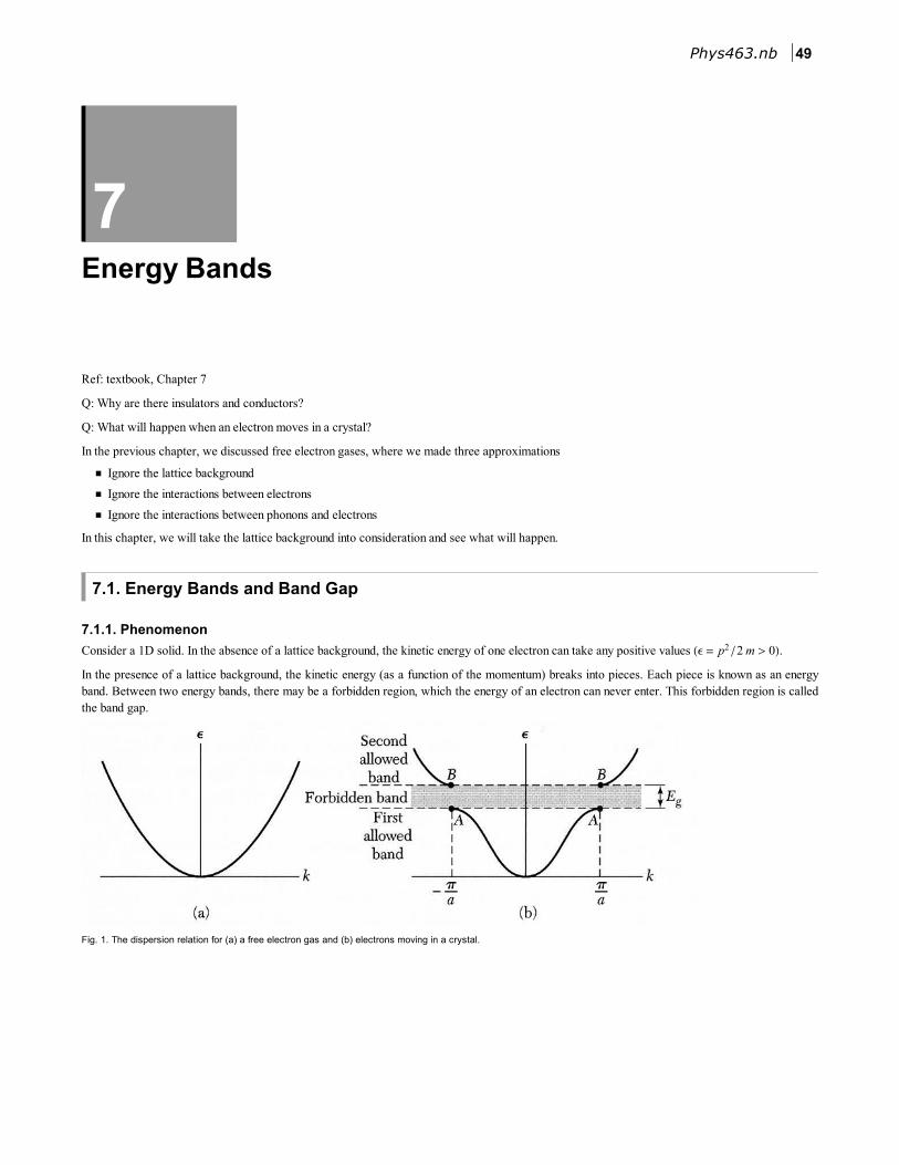
Consider a 1D solid. In the absence of a lattice background, the kinetic energy of one electron can take any positive values HΕ = p2 � 2 m > 0L.
In the presence of a lattice background, the kinetic energy (as a function of the momentum) breaks into pieces. Each piece is known as an energy
band. Between two energy bands, there may be a forbidden region, which the energy of an electron can never enter. This forbidden region is called
the band gap.
Fig. 1. The dispersion relation for (a) a free electron gas and (b) electrons moving in a crystal.
Phys463.nb 49
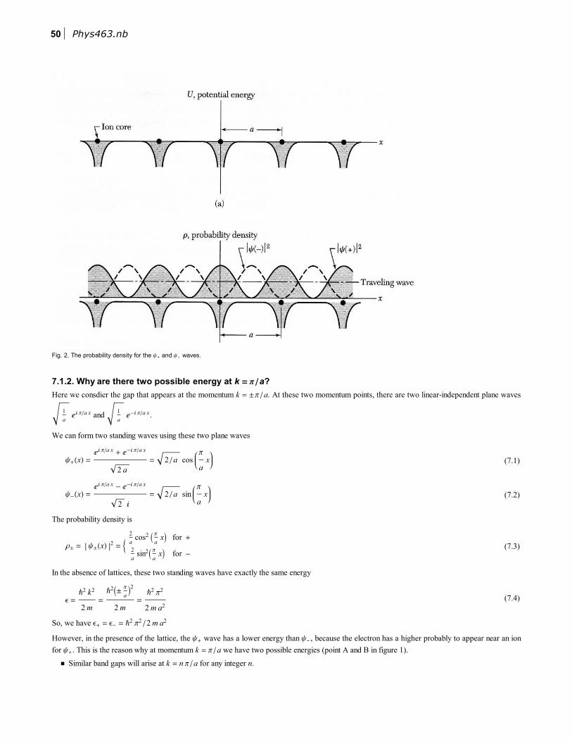
Fig. 2. The probability density for the Ψ+ and Ψ- waves.
7.1.2. Why are there two possible energy at k = Π �a?
Here we consdier the gap that appears at the momentum k = ± Π � a. At these two momentum points, there are two linear-independent plane waves
1
aãä Π�a x
and 1
aã-ä Π�a x
.
We can form two standing waves using these two plane waves
(7.1)Ψ+HxL =ãä Π�a x + ã-ä Π�a x
2 a
= 2 � a cos
Π
a
x
(7.2)Ψ-HxL =ãä Π�a x - ã-ä Π�a x
2 ä
= 2 � a sin
Π
a
x
The probability density is
(7.3)Ρ± = Ψ±HxL 2= :
2
acos
2 I Π
axM for +
2
asin
2I Π
axM for -
In the absence of lattices, these two standing waves have exactly the same energy
(7.4)Ε =Ñ
2k
2
2 m
=
Ñ2I±
Π
aM2
2 m
=Ñ
2 Π2
2 m a2
So, we have Ε+ = Ε- = Ñ2 Π2 � 2 m a
2
However, in the presence of the lattice, the Ψ+ wave has a lower energy than Ψ-, because the electron has a higher probably to appear near an ion
for Ψ+. This is the reason why at momentum k = Π � a we have two possible energies (point A and B in figure 1).
� Similar band gaps will arise at k = n Π � a for any integer n.
50 Phys463.nb
� The momentum region -nΠ
a< k < -Hn - 1L Π
a and Hn - 1L Π
a< k < n
Π
a is called the nth Brillouin zones (This is the same Brillouin zones as
we learned in the reciprocal lattice).
� In side the of these Brillouin zones, the energy is a smooth function and this smooth function is called the nth band.
� At each boundary of the Brillouin zones, the energy curve shows a jump and thus an energy gap opens up.
7.1.3. Magnitude of the band gap
The size of the gap can be estimated as the following
(7.5)Eg = à0
a
UHxL Ρ+HxL â x - à0
a
UHxL Ρ+HxL Ρ-HxL â x
where UHxL is the potential energy from the ions. Because the lattice is periodic, UHxL is a periodic function UHx + aL = UHxL where a is the lattice
constant. In addition, with out loss of generality, we can assume that UHxL is an even function U HxL = -UHxL.For such an even periodic function, we can write it as a a Fourier series.
(7.6)UHxL =U0
2
+ ânUn cos
2 Π n
a
x
and
(7.7)Un =2
aà
0
a
UHxL cos
2 Π n
a
x â x
The energy gap at k = ± Π � a is
(7.8)Eg = à0
a
UHxL@Ρ+HxL - Ρ-HxLD â x =2
aà
0
a
UHxLBcos2
Π
a
x - sin2
Π
a
x F â x =2
aà
0
a
UHxL cos
2 Π
a
x â x = U1
The energy gap at k = ±n Π � a is
(7.9)Eg = à0
a
UHxL@Ρ+HxL - Ρ-HxLD â x =2
aà
0
a
UHxLBcos2
n
Π
a
x - sin2
n
Π
a
x F â x =2
aà
0
a
UHxL cos
2 Π
a
n x â x = Un
7.2. Bloch waves
7.2.1. The effect of the lattice potential: the Hamiltonian and the Schrodinger equation
The Hamiltonian
(7.10)H =p
2
2 m
+ UHxL = -Ñ
2
2 m
¶x2
+UHxLThe Schrodinger equation
(7.11)-Ñ
2
2 m
¶x2
ΨHxL + UHxL ΨHxL = Ε ΨHxLThis equation is in general hard (or impossible) to solve analytically. However, F. Bloch managed to prove a very important theorem, which states
that the solution to this equation must take the following form:
(7.12)ΨkHxL = ukHxL ãä k x
Here, uHxL is a periodic function ukHx + aL = ukHxL, which has the same period as the lattice.
� This conclusion is true in any dimensions. For example, in 3D, we have ΨJr®N = u
k
®Jr®N expKä k
®
× r®O where uJr
®N is a 3D periodic function
uk
®Jr®N = u
k
®Kr®
+ T
®O where T
®
is any lattice vector.
This type of waves are known as the Bloch wave. They have some nice properties
� The plane waves are a special type of Bloch waves with the function uHxL = constant.
Phys463.nb 51
� The Bloch wave is NOT an eigenstate of the momentum operator. In other words, it doesn’t have a well-defined momentum (unless
uHxL = constant). However, the parameter k
®
in the Bloch wave behaves very similarly to the momentum. We call Ñ k
®
the lattice momentum.
� Lattice momentum is not the momentum, but it is conserved in a lattice.
7.2.2. The proof of the Bloch theorem
Define the translation operator
(7.13)Ta ΨHrL = ΨHr + aLwhere a is the lattice constant. This operator shift our quantum system in real space by the lattice constant a.
Under translation by a, a quantum operator O changes as O ® Ta O Ta-1
. Therefore, for the Hamiltonian
(7.14)Ta HHxL Ta-1
= HHx + aLBecause
(7.15)HHxL = -Ñ
2
2 m
¶x2
+UHxLand
(7.16)HHx + aL = -Ñ
2
2 m
¶x2
+UHx + aL = -Ñ
2
2 m
¶x2
+UHxLwe know immediately that H HxL = HHx + aL. And thus
(7.17)Ta HHxL Ta-1
= HHx + aL = HHxLIn other words,
(7.18)Ta HHxL = HHxL Ta
so
(7.19)@Ta, HD = 0
If two operators commute, we know that we can find common eigenstates of these two operators. For Ta and H, this means that we can find a set
of (complete orthonormal) basis ΨkHxL, such that
(7.20)H ΨkHxL = Ε ΨkHxL and Ta ΨkHxL = ãä k a
ΨkHxLHere, we used the fact that H is an Hermitian operator, so that its eigenvalues Ε must be real. For Ta, because it is a unitary operator, its eigenvalue
must be a complex with absolute value 1.
Define
(7.21)ukHxL = ã-ä k x
ΨkHxLIt is easy to prove that ukHxL is a periodic function ukHxL = ukHx + aL.
(7.22)ukHx + aL = ã-ä k Hx+aL
ΨkHx + aL = ã-ä k Hx+aL
Ta ΨkHxL = ã-ä k Hx+aL
ãä k a
ΨkHxL = ã-ä k x
ΨkHxL = ukHxLTherefore,
(7.23)ΨkHxL = ukHxL ãä k x
where ukHxL is a periodic function.
7.3. Properties of Bloch waves and crystal momentum
Eigen wave functions for a single particle moving in a periodic potential: Bloch waves
(7.24)ΨnkHxL = un kHxL ã
ä k x
Here k is known as the crystal momentum. The corresponding eigenenergy is Εn,k , which satisfies
52 Phys463.nb
(7.25)H Ψn,kHxL = Εn,k Ψn,k
HxL
7.3.1. value of k?
� The crystal momenta are only well-defined modulo G, where G is a reciprocal vector.
� Therefore, we can limit the crystal momentum to the first Brillouin zone without loss of information (e.g. for a 1D system, -Π � a £ k < Π � a).
Proof : Suppose we have a Bloch wave with crystal momentum k
(7.26)Ψn kHxL = un kHxL ãä k x
Define k ' = k + G
(7.27)Ψn kHxL = un kHxL ãä k x
= un k '-GHxL ãä Hk '-G L x
= un k '-GHxL ã-ä G x
ãä k ' x
Define un k 'HxL = un, k '-GHxL ã-ä G x,
(7.28)Ψn kHxL = un k '-GHxL ã-ä G x
ãä k ' x
= un k 'HxL ãä k ' x
It is easy to check that un,k 'HxL = un,k 'Hx + TL where T is any lattice vector.
(7.29)un,k 'Hx + TL = un, k '-GHx + TL ã-ä G Hx+TL
= un, k '-GHxL ã-ä G x
= un,k 'HxLTherefore, Ψn kHxL = un k 'HxL ãä k ' x
is also a Bloch wave function with crystal momentum k '
(7.30)Ψn kHxL = un k 'HxL ãä k ' x
= Ψn,k 'HxLConclusion: as long as k and k ' differs by a reciprocal lattice vector G, we can write a Bloch wavefunction with crystal momentum k as a Bloch
wavefunction with crystal momentum k '.
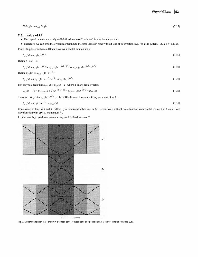
In other words, crystal momentum is only well defined modulo G
Fig. 3. Dispersion relation ΕnHkL shown in extended zone, reduced zone and periodic zone. (Figure 4 in text book page 225).
Phys463.nb 53
7.3.2. Reduced Brillouin zone
Since the crystal momentum is only well defined modulo G, we can limit the momentum to the first Brillouin zone (e.g. for a 1D system,
-Π � a £ k < Π � a) without loss of information.
We can plot the eigen-energy Εn,k as a function of k in the first Brillouin zone. This way of plotting Εn,k is known as the reduced Brillouin zone (See
figure b above)
The band index n is (from bottom to top) n = 1, 2, 3, …
7.3.3. Periodic Brillouin zone
There is another way of plotting Εn,k . We can start from the reduced Brillouin zone and then we plot Εn,k as a periodic function of k, repeating the
same curve in the second, third, ... Brillouin zone (See figure c above)
7.3.4. Folding, Reduced Brillouin zone and extended Brillouin zone for free particles without lattices
We know that plane waves is a special case of Bloch waves (where the periodic potential is V = 0). Therefore, we can present the dispersion of a
free particle Ε = Ñ2
k2 � 2 m in the same way (in the reduced BZ and periodic BZ).
The can be achieve using the following procedures:
start from the dispersion ΕHkL = Ñ2
k2 � 2 m,
then move the curve in the regions H2 n - 1L Π � a < k < 2 n Π � a to -Π � a < k < 0 and move the curve in the regions 2 n Π � a < k < H2 n + 1L Π � a to
0 < k < Π � a.
So we get the figure below.
Fig. 4. Reduced zone for a free particle. (textbook p 177 Fig. 8)
This construction is known as Brillouin zone folding. Similarly, the reverse procedure is known as “unfolding”. We can unfold the reduced
Brillouin zone to get the “extended Brillouin zone”, going back to the case -¥ < k < +¥ and get one single curve with k2 � 2 m for a free particle.
54 Phys463.nb
7.3.5. Folding, Reduced Brillouin zone and extended Brillouin zone for free particles without lattices
In the presence of a lattice, we can also “unfold” the extended Brillouin zone to get an extended Brillouin zone. (see figure 3.a above).
Extended zone is often used when the lattice potential is very weak and thus can be treated as a small perturbation. The dispersion in extended
zone is close to k2 � 2 m dispersion of a free particle (without a lattice background). So when lattice is very weak, we can use this extended zone to
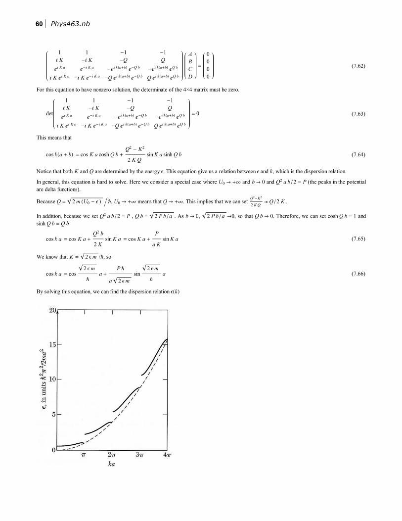
see how the k2 � 2 m dispersion evolves into the band structure of ΕnHkL.
7.4. Why we have two different types of materials: conductors and insulators?
7.4.1. Definition of conductors and insulators.
� In real life, we call materials with very large resistivity Ρ insulators and materials with very small Ρ conductors. This is NOT a rigorous
(scientific) definition, because it doesn’t provide a sharp boundary between conductors and insulators.
� In physics, we use the T ® 0 limit of the resistivity to define insulators and conductors. This is a sharp (rigorous) definition with no ambiguity
(at least mathematically speaking).
Consider the resistivity as a function of temperature ΡHTL. If the resistivity diverges in the T ® 0 limit, the system is an insulator. If the resistivity
converge to a finite value, the system is a conductor.
(7.31)LimT®0 ΡHTL = : ¥ insulators
Ρ0 conductors
� Strictly speaking, we can only distinguish insulators from conductors at T = 0. The value of Σ at room temperature doesn’t matter in this
definition.
� In practice, one cannot really reach T = 0. So we go to very low T, and check whether the resistivity increases or decreases as T is reduced.
If Ρ increases exponentially as T goes down, Ρ µ expHD � kB TL, we say that the system is an insulator.
� Why exponential? This will be answered at the end of this section.
7.4.2. Conductors and insulators from energy bands
For weakly-correlated materials (where electron-electron plays no essential role):
� If a material has partially filled bands, it is a conductor.
� If a material only has fully filled bands, it is an insulator.
This is because only partially filled bands can have conductivity.
Another way to present the same statement
� If the Fermi energy (zero temperature chemical potential) of a material crosses with one or more bands, it is a conductor.
� If the Fermi energy (zero temperature chemical potential) of a material is inside the energy gap and doesn’t cross with any bands, it is an
insulator.
7.4.3. Partially filled bands
Equation of motion for electrons (as we learned in the previous chapter):
(7.32)â p
®
â t
= -e E
®
-p®
- p0
®
Τ
where Τ is the collision time (the relaxation time)
(7.33)â k
®
â t
= -e E
®
Ñ
-k
®
- k0
®
Τ
For Bloch waves, k is the crystal momentum. From this equation, we find that if we apply an electric field, electrons increase their crystal
momentum (moving to the -E
®
direction). If we wait long enough time, the system shall reach the static limit, âk
®
ât= 0, so that
(7.34)0 =
â k
®
â t
= -e E
®
Ñ
-k
®
- k0
®
Τ
Phys463.nb 55
So
(7.35)∆k
®
= k
®
- k0
®
= -e E
®
Ñ
Τ
For a partially filled bands, this implies that total momentum of all electrons will be non-zero if E ¹ 0. So we got a electric current. Since an E-field
induces an electric current in this material, this is an conductor.
7.4.4. Fully filled bands
For a fully filled bands, if we apply an E-field, electrons also changes its momentum. But now, because the band is fully filled, after we change the
crystal momentum of all the electrons, we still have a fully filled band and thus the total momentum is still zero.
NO CURRENT after we applies an E-field. So a filled band doesn’t contribute to conductivity.
If a material only have filled bands, it is an insulator.
7.4.5. Valence band and conduction band
Fully filled bands are called the valence bands. Partially filled bands or empty bands are called conduction bands.
Please notice that although an empty band is also called a conduction band, it doesn’t contribute anything to conductivity at T = 0.
7.4.6. How many electrons can one band host?
# of quantum states (the factor 2 comes from spin-1/2)
(7.36)
2 à âdp
H2 Π ÑLd �V
= 2 à âdk
H2 Π Ld �V
= 2
Volume of one BZ
H2 ΠLd �V
=2
H2 ΠLd
Volume of one BZ ´ Volume of the system =
2
H2 ΠLd
Volume of one BZ ´ HVolume of one unit cell ´ number of unit cellsL =
2
Volume of one BZ ´ Volume of one unit cell
H2 ΠLd
´ number of unit cells = 2 ´ number of unit cells
Number of electrons in a fully filled band: 2 per unit cell.
This implies immediately that for weakly interacting materials, in which electron-electron interactions plays no essential role, even number of
electrons per unit cell is a necessary condition for a band insulator, but it is NOT sufficient.
� If a material has odd number of electrons per unit cell (ignore interactions), it must be a conductor.
� If a material has even number of electrons per unit cell (ignore interactions), it may be a metal or an insulator.
� Band insulators must have even number of electrons per unit cell.
� This conclusion is only true for weakly correlated systems. For strongly correlated materials, one can get an insulator with odd number of
electrons per unit cell (e.g. the Mott insulator in high Tc compounds).
7.4.7. Semi-conductors and semi-metals
Semi-conductors are actually insulator, but their gaps are small (compare to “good” insulators like glass, rubber, plastics). Because their gap is
very small, these insulator are not far away from a metal. If we can adjust the chemical potential by a little bit, we can turn this insulators into an
conductor. This property is very useful for computer technology. There, a conducting state means 1 and an insulating state means 0. For a
computer, we want each bit to switch back and forth between 0 and 1 (as fast as possible and as easy as possible). So we want a system on the
verge of a insulator-conductor transition, such that we can turn the system back and forth across this boundary easily.
Semi-metals are actually conductors, but they are not very far away from an insulator. Due to historical reasons, this terminology has been used to
refer to two different types materials.
This first class of semi-metals are also known as the “indirect gap semiconductor”. For this material, at each momentum point, the conducting and
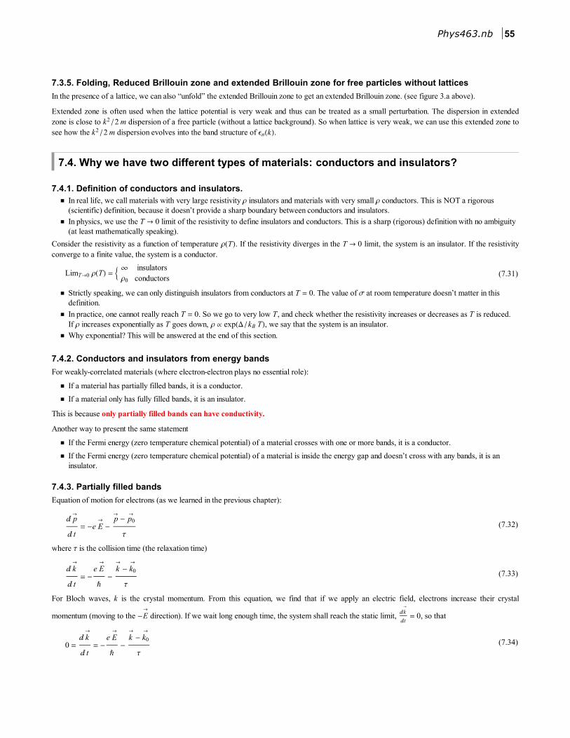
valence band has a gap but there is no turn insulating gap when we taken all momentum into account. See figure b below.
56 Phys463.nb
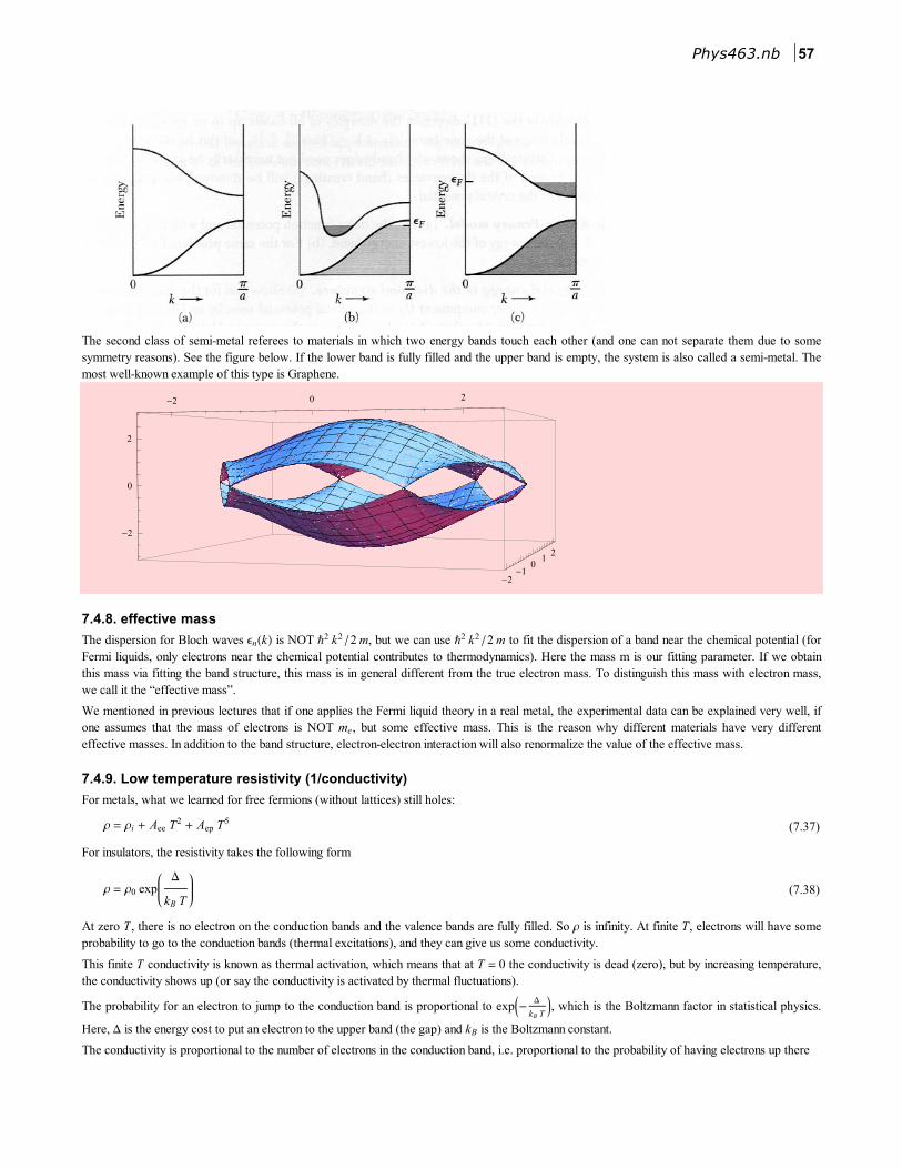
The second class of semi-metal referees to materials in which two energy bands touch each other (and one can not separate them due to some
symmetry reasons). See the figure below. If the lower band is fully filled and the upper band is empty, the system is also called a semi-metal. The
most well-known example of this type is Graphene.
-2 0 2
-2-1
01
2
-2
0
2
7.4.8. effective mass
The dispersion for Bloch waves ΕnHkL is NOT Ñ2
k2 � 2 m, but we can use Ñ
2k
2 � 2 m to fit the dispersion of a band near the chemical potential (for
Fermi liquids, only electrons near the chemical potential contributes to thermodynamics). Here the mass m is our fitting parameter. If we obtain
this mass via fitting the band structure, this mass is in general different from the true electron mass. To distinguish this mass with electron mass,
we call it the “effective mass”.
We mentioned in previous lectures that if one applies the Fermi liquid theory in a real metal, the experimental data can be explained very well, if
one assumes that the mass of electrons is NOT me, but some effective mass. This is the reason why different materials have very different
effective masses. In addition to the band structure, electron-electron interaction will also renormalize the value of the effective mass.
7.4.9. Low temperature resistivity (1/conductivity)
For metals, what we learned for free fermions (without lattices) still holes:
(7.37)Ρ = Ρi + Aee T2
+ Aep T5
For insulators, the resistivity takes the following form
(7.38)Ρ = Ρ0 exp
D
kB T
At zero T, there is no electron on the conduction bands and the valence bands are fully filled. So Ρ is infinity. At finite T, electrons will have some
probability to go to the conduction bands (thermal excitations), and they can give us some conductivity.
This finite T conductivity is known as thermal activation, which means that at T = 0 the conductivity is dead (zero), but by increasing temperature,
the conductivity shows up (or say the conductivity is activated by thermal fluctuations).
The probability for an electron to jump to the conduction band is proportional to expJ-D
kB TN, which is the Boltzmann factor in statistical physics.
Here, D is the energy cost to put an electron to the upper band (the gap) and kB is the Boltzmann constant.
The conductivity is proportional to the number of electrons in the conduction band, i.e. proportional to the probability of having electrons up there
Phys463.nb 57
(7.39)Σ µ number of electrons in the conduction band µ exp -D
kB T
So the resistivity is its inverse
(7.40)Ρ =1
Σµ exp
D
kB T
In experiments, one can measure Ρ at different temperature and then plot ln Ρ as a function of 1 � T. This plot should be a straight line for an
insulator, and the slope is the energy gap D.
7.5. Kronig-Penney model
7.5.1. The model
Here we consider a special potential where
(7.41)UHxL = : 0 0 < x < a
U0 -b < x < 0
Fig. 5. Potential Energy
For this potential, we can solve the Schrodinger equation in the region 0 < x < a and -b < x < 0 separately and they try to match to boundary
conditions at x = 0 and a.
(7.42)-Ñ
2
2 m
¶x2
ΨHxL + UHxL ΨHxL = Ε ΨHxL
7.5.2. Eigenstates with eigen-energy Ε
For 0 < x < a, UHxL = 0, so
(7.43)-Ñ
2
2 m
¶x2
ΨHxL = Ε ΨHxLThe solution contains two plane waves with wave vector K and -K
(7.44)Ψ1HxL = A ãä K x
+ B ã-ä K x
The wavevector is determined by the Schrodinger equation, which says
(7.45)
Ñ2
K2
2 m
ΨHxL = Ε ΨHxL
So we have K = 2 m Ε � Ñ
For -b < x < 0, U HxL = U0, so
58 Phys463.nb
(7.46)-Ñ
2
2 m
¶x2
ΨHxL + U0 ΨHxL = Ε ΨHxLThe solution of this differential equation is
(7.47)Ψ2HxL = C ãQ x
+ D ãQ x
where Q is determined by the Schrodinger equation, which says
(7.48)U0 -Ñ
2Q
2
2 m
ΨHxL = Ε ΨHxLSo we have
(7.49)Q = 2 m HU0 - Ε L �Ñ
7.5.3. Boundary conditions at x = 0
At x = 0, we know that the wave function must be a continuous function and the first order derivative of the wavefunction must also be a continu-