ENERGY CONSERVATION AND ONSAGER’S ...homepages.math.uic.edu/~shvydkoy/papers/onsager.pdfENERGY...

ENERGY CONSERVATION AND ONSAGER’S CONJECTUREFOR THE EULER EQUATIONS

A. CHESKIDOV, P. CONSTANTIN, S. FRIEDLANDER, AND R. SHVYDKOY

ABSTRACT. Onsager conjectured that weak solutions of the Euler equa-tions for incompressible fluids in R3 conserve energy only if they have acertain minimal smoothness, (of order of 1/3 fractional derivatives) andthat they dissipate energy if they are rougher. In this paper we provethat energy is conserved for velocities in the function space B

1/33,c(N). We

show that this space is sharp in a natural sense. We phrase the energyspectrum in terms of the Littlewood-Paley decomposition and show thatthe energy flux is controlled by local interactions. This locality is shownto hold also for the helicity flux; moreover, every weak solution of theEuler equations that belongs to B

2/33,c(N) conserves helicity. In contrast,

in two dimensions, the strong locality of the enstrophy holds only in theultraviolet range.

1. INTRODUCTION

The Euler equations for the motion of an incompressible inviscid fluidare

(1)∂u

∂t+ (u · ∇)u = −∇p,

(2) ∇ · u = 0,

where u(x, t) denotes the d-dimensional velocity, p(x, t) denotes the pres-sure, and x ∈ Rd. We mainly consider the case d = 3. When u(x, t) is aclassical solution, it follows directly that the total energy E(t) = 1

2

∫ |u|2 dxis conserved. However, conservation of energy may fail for weak solutions(see Scheffer [27], Shnirelman [26]). This possibility has given rise to aconsiderable body of literature and it is closely connected with statisticaltheories of turbulence envisioned 60 years ago by Kolmogorov and On-sager. For reviews see, for example, Eyink and Sreenivasan [16], Robert[25], and Frisch [17].

Date: April 3, 2007.2000 Mathematics Subject Classification. Primary: 76B03; Secondary: 76F02.Key words and phrases. Euler equations, anomalous dissipation, energy flux, Onsager

conjecture, turbulence, Littlewood-Paley spectrum.1

2 A. CHESKIDOV, P. CONSTANTIN, S. FRIEDLANDER, AND R. SHVYDKOY

Onsager [24] conjectured that in 3-dimensional turbulent flows, energydissipation might exist even in the limit of vanishing viscosity. He sug-gested that an appropriate mathematical description of turbulent flows (inthe inviscid limit) might be given by weak solutions of the Euler equationsthat are not regular enough to conserve energy. According to this view, non-conservation of energy in a turbulent flow might occur not only from vis-cous dissipation, but also from lack of smoothness of the velocity. Specif-ically, Onsager conjectured that weak solutions of the Euler equation withHolder continuity exponent h > 1/3 do conserve energy and that turbulentor anomalous dissipation occurs when h ≤ 1/3. Eyink [14] proved energyconservation under a stronger assumption. Subsequently, Constantin, E andTiti [9] proved energy conservation for u in the Besov space Bα

3,∞, α > 1/3.More recently the result was proved under a slightly weaker assumption byDuchon and Robert [13].

In this paper we sharpen the result of [9] and [13]: we prove that energy isconserved for velocities in the Besov space of tempered distributions B

1/33,p .

In fact we prove the result for velocities in the slightly larger space B1/33,c(N)

(see Section 3). This is a space in which the “Holder exponent” is exactly1/3, but the slightly better regularity is encoded in the summability condi-tion. The method of proof combines the approach of [9] in bounding thetrilinear term in (3) with a suitable choice of the test function for weak so-lutions in terms of a Littlewood-Paley decomposition. Certain cancelationsin the trilinear term become apparent using this decomposition. We observethat the space B

1/33,c(N) is sharp for our argument by giving an example of a

divergence free vector field in B1/33,∞ for which the energy flux due to the tri-

linear term is bounded from below by a positive constant. This constructionfollows ideas in [14]. However, because it is not a solution of the unforcedEuler equation, the example does not prove that indeed there exist unforcedsolutions to the Euler equation that live in B

1/33,∞ and dissipate energy.

Experiments and numerical simulations indicate that for many turbu-lent flows the energy dissipation rate appears to remain positive at largeReynolds numbers. However, there are no known rigorous lower boundsfor slightly viscous Navier-Stokes equations. The existence of a Holder-continuous weak solution of Euler’s equation that does not conserve en-ergy remains an open question. For a discussion see, for example, Duchonand Robert [13], Eyink [14], Shnirelman [27], Scheffer [26], de Lellis andSzekelyhidi [12].

We note that the proof in Section 3 applied to Burger’s equation for 1-dimensional compressible flow gives conservation of energy in B

1/33,c(N). In

ENERGY CONSERVATION 3

this case it is easy to show that conservation of energy can fail in B1/33,∞

which is the sharp space for shocks.The Littlewood-Paley approach to the issue of energy conservation ver-

sus turbulent dissipation is mirrored in a study of a discrete dyadic modelfor the forced Euler equations [5, 6]. By construction, all the interactionsin that model system are local and energy cascades strictly to higher wavenumbers. There is a unique fixed point which is an exponential global at-tractor. Onsager’s conjecture is confirmed for the model in both directions,i.e. solutions with bounded H5/6 norm satisfy the energy balance condi-tion and turbulent dissipation occurs for all solutions when the H5/6 normbecomes unbounded, which happens in finite time. The absence of anoma-lous dissipation for inviscid shell models has been obtained in [10] in aspace with regularity logarithmically higher than 1/3.

In Section 3.2 we present the definition of the energy flux employed inthe paper. This is the flux of the Littlewood-Paley spectrum (see [7]), whichis a mathematically convenient variant of the physical concept of flux fromthe turbulence literature. Our estimates employing the Littlewood-Paley de-composition produce not only a sharpening of the conditions under whichthere is no anomalous dissipation, but also provide detailed informationconcerning the cascade of energy flux through frequency space. In section3.3 we prove that the energy flux through the sphere of radius κ is con-trolled primarily by frequencies of order κ. Thus we give a mathematicaljustification for the physical intuition underlying much of turbulence the-ory, namely that the flux is controlled by local interactions (see, for exam-ple, Kolmogorov [18] and also [15], where sufficient conditions for localitywere described). Our analysis makes precise an exponential decay of non-local contributions to the flux that was conjectured by Kraichnan [19].

The energy is not the only scalar quantity that is conserved under evolu-tion by classical solutions of the Euler equations. For 3-dimensional flowsthe helicity is an important quantity related to the topological configura-tions of vortex tubes (see, for example, Moffatt and Tsinober [23]). Thetotal helicity is conserved for smooth ideal flows. In Section 4 we observethat the techniques used in Section 3 carry over exactly to considerations ofthe helicity flux, i.e., there is locality for turbulent cascades of helicity andevery weak solution of the Euler equation that belongs to B

2/33,c(N) conserves

helicity. This strengthens a recent result of Chae [2]. Once again our argu-ment is sharp in the sense that a divergence free vector field in B

2/33,∞ can be

constructed to produce an example for which the helicity flux is boundedfrom below by a positive constant.


An important property of smooth flows of an ideal fluid in two dimen-sions is conservation of enstrophy (i.e. the L2 norm of the curl of the ve-locity). In section 4.2 we apply the techniques of Section 3 to the weakformulation of the Euler equations for velocity using a test function thatpermits estimation of the enstrophy. We obtain the result that, unlike thecases of the energy and the helicity, the locality in the enstrophy cascade isstrong only in the ultraviolet range. In the infrared range there are nonlo-cal effects. Such ultraviolet locality was predicted by Kraichnan [20] andagrees with numerical and experimental evidence. Furthermore, there arearguments in the physical literature that hold that the enstrophy cascade isnot local in the infrared range. We present a concrete example that exhibitsthis behavior.

In the final section of this paper, we study the bilinear term B(u, v). Weshow that the trilinear map (u, v, w) → 〈B(u, v), w)〉 defined for smoothvector fields in L3 has a unique continuous extension to B1/2

18/7,23 (and afortiori to H5/63, which is the relevant space for the dyadic model prob-lem referred to above). We present an example to show that this result isoptimal. We stress that the borderline space for energy conservation is muchrougher than the space of continuity for 〈B(u, v), w〉.

2. PRELIMINARIES

We will use the notation λq = 2q (in some inverse length units). LetB(0, r) denote the ball centered at 0 of radius r in Rd. We fix a nonnegativeradial function χ belonging to C∞

0 (B(0, 1)) such that χ(ξ) = 1 for |ξ| ≤1/2. We further define

(3) ϕ(ξ) = χ(λ−11 ξ)− χ(ξ).

Then the following is true

(4) χ(ξ) +∑q≥0

ϕ(λ−1q ξ) = 1,

and

(5) |p− q| ≥ 2 ⇒ Supp ϕ(λ−1q ·) ∩ Supp ϕ(λ−1

p ·) = ∅.

We define a Littlewood-Paley decomposition. Let us denote by F theFourier transform on Rd. Let h, h, ∆q (q ≥ −1) be defined as follows:


h = F−1ϕ and h = F−1χ,

∆qu = F−1(ϕ(λ−1q ξ)Fu) = λd

q

∫h(λqy)u(x− y)dy, q ≥ 0

∆−1u = F−1(χ(ξ)Fu) =

∫h(y)u(x− y)dy.

For Q ∈ N we define

(6) SQ =

Q∑q=−1

∆q.

Due to (3) we have

(7) SQu = F−1(χ(λ−1Q+1ξ)Fu).

Let us now recall the definition of inhomogeneous Besov spaces.

Definition 2.1. Let s ∈ R, and 1 ≤ p, r ≤ ∞. The inhomogeneous Besovspace Bs

p,r is the space of tempered distributions u such that the norm

‖u‖Bsp,r

def= ‖∆−1u‖Lp +

∥∥∥(λs

q‖∆qu‖Lp

)q∈N

∥∥∥`r(N)

is finite.

We refer to [3] and [21] for background on harmonic analysis in the con-text of fluids. We will use the following Bernstein inequalities.

Lemma 2.2.

‖∆qu‖Lb ≤ λd( 1

a− 1

b)

q ‖∆qu‖La for b ≥ a ≥ 1.

As a consiquence we have the following inclusions.

Corollary 2.3. If b ≥ a ≥ 1, then we have the following continuous em-beddings

Bsa,r ⊂ B

s−d

(1a− 1

b

)

b,r ,(8)

B0a,2 ⊂ La, for a ≥ 2.(9)

In particular, the following chain of inclusions will be used throughoutthe text.

(10) H56 (R3) ⊂ B

2394,2(R3) ⊂ B

12187

,2(R3) ⊂ B

133,2(R3).


3. ENERGY FLUX AND LOCALITY

3.1. Weak solutions.

Definition 3.1. A function u is a weak solution of the Euler equations withinitial data u0 ∈ L2(Rd) if u ∈ Cw([0, T ]; L2(Rd)), (the space of weaklycontinuous functions in time) and for every ψ ∈ C1([0, T ];S(Rd)) withS(Rd) the space of rapidly decaying functions, with ∇x · ψ = 0 and 0 ≤t ≤ T , we have(11)

(u(t), ψ(t))− (u(0), ψ(0))−∫ t

0

(u(s), ∂sψ(s))ds =

∫ t

0

b(u, ψ, u)(s)ds,

where

(u, v) =

∫

Rd

u · vdx,

b(u, v, w) =

∫

Rd

u · ∇v · w dx,

and ∇x · u(t) = 0 in the sense of distributions for every t ∈ [0, T ].

Clearly, (11) implies Lipschitz continuity of the maps t → (u(t), ψ) forfixed test functions. By an approximation argument one can show that forany weak solution u of the Euler equation, the relationship (11) holds for allψ that are smooth and localized in space, but only weakly Lipschitz in time.This justifies the use of physical space mollifications of u as test functionsψ. Because we do not have an existence theory of weak solutions, this is arather academic point.

3.2. Energy flux. For a divergence-free vector field u ∈ L2 we introducethe Littlewood-Paley energy flux at wave number λQ by

(12) ΠQ =

∫

R3

Tr[SQ(u⊗ u) · ∇SQu]dx.

If u(t) is a weak solution to the Euler equation, then substituting the testfunction ψ = S2

Qu into the weak formulation of the Euler equation (11) weobtain

(13) ΠQ(t) =1

2

d

dt‖SQu(t)‖2

2.

Let us introduce the following localization kernel

(14) K(q) =

λ

2/3q , q ≤ 0;

λ−4/3q , q > 0,


For a tempered distribution u in R3 we denote

dq = λ1/3q ‖∆qu‖3,(15)

d2 = d2qq≥−1.(16)

Proposition 3.2. The energy flux of a divergence-free vector field u ∈ L2

satisfies the following estimate

(17) |ΠQ| ≤ C(K ∗ d2)3/2(Q),

where C > 0 is an absolute constant.

The proof of Proposition 3.2 will be given later in this section. From (17)we immediately obtain

(18) lim supQ→∞

|ΠQ| ≤ lim supQ→∞

d3Q.

We define B1/33,c(N) to be the class of all tempered distributions u in R3 for

which

(19) limq→∞

λ1/3q ‖∆qu‖3 = 0,

and hence dq → 0. We endow B1/33,c(N) with the norm inherited from B

1/33,∞.

Notice that the Besov spaces B1/33,p for 1 ≤ p < ∞, and in particular B

1/33,2

are included in B1/33,c(N).

As a consequence of (13) and (18) we obtain the following theorem.

Theorem 3.3. The total energy flux of any divergence-free vector field inthe class B

1/33,c(N) ∩ L2 vanishes. In particular, every weak solution to the

Euler equation that belongs to the class L3([0, T ]; B1/33,c(N)) ∩Cw([0, T ]; L2)

conserves energy.

Remark 3.4. We note that (13) and (18) imply that every weak solution uto the Euler equations on [0, T ] conserves energy provided the followingweaker condition holds

limq→∞

∫ T

0

λq‖∆qu‖33 dt = 0.

Spaces defined by similar conditions were used in [4, 8].

Proof of Proposition 3.2. In the argument below all the inequalities shouldbe understood up to a constant multiple.

Following [9] we write

(20) SQ(u⊗ u) = rQ(u, u)− (u− SQu)⊗ (u− SQu) + SQu⊗ SQu,


where

rQ(u, u) =

∫

R3

hQ(y)(u(x− y)− u(x))⊗ (u(x− y)− u(x))dy,

hQ(y) = λ3Q+1h(λQ+1y).

After substituting (20) into (12) we find

ΠQ =

∫

R3

Tr[rQ(u, u) · ∇SQu]dx(21)

−∫

R3

Tr[(u− SQu)⊗ (u− SQu) · ∇SQu]dx.(22)

We can estimate the term in (21) using the Holder inequality by

‖rQ(u, u)‖3/2‖∇SQu‖3,

whereas

(23) ‖rQ(u, u)‖3/2 ≤∫

R3

∣∣∣hQ(y)∣∣∣ ‖u(· − y)− u(·)‖2

3dy.

Let us now use Bernstein’s inequalities and Corollary 2.3 to estimate

‖u(· − y)− u(·)‖23 ≤

∑q≤Q

|y|2λ2q‖∆qu‖2

3 +∑q>Q

‖∆qu‖23(24)

= λ4/3Q |y|2

∑q≤Q

λ−4/3Q−q d2

q + λ−2/3Q

∑q>Q

λ2/3Q−qd

2q(25)

≤ (λ4/3Q |y|2 + λ

−2/3Q )(K ∗ d2)(Q).(26)

Collecting the obtained estimates we find∣∣∣∣∫

R3

Tr[rQ(u, u) · ∇SQu]dx

∣∣∣∣

≤ (K ∗ d2)(Q)

(∫

R3

∣∣∣hQ(y)∣∣∣ λ

4/3Q |y|2dy + λ

−2/3Q

) [∑q≤Q

λ2q‖∆qu‖2

3

]1/2

≤ (K ∗ d2)(Q)λ−2/3Q

[∑q≤Q

λ4/3q d2

q

]1/2

≤ (K ∗ d2)3/2(Q)


Analogously we estimate the term in (22)∫

R3

Tr[(u− SQu)⊗ (u− SQu) · ∇SQu]dx

≤ ‖u− SQu‖23‖∇SQu‖3

≤(∑

q>Q

‖∆qu‖23

)(∑q≤Q

λ2q‖∆qu‖2

3

)1/2

≤ (K ∗ d2)3/2(Q).

This finishes the proof.¤

3.3. Energy flux through dyadic shells. Let us introduce the energy fluxthrough a sequence of dyadic shells between scales −1 ≤ Q0 < Q1 < ∞as follows

(27) ΠQ0Q1 =

∫

R3

Tr[SQ0Q1(u⊗ u) · ∇SQ0Q1u] dx,

where

(28) SQ0Q1 =∑

Q0≤q≤Q1

∆q = SQ1 − SQ0 .

If u is a weak solution of the Euler equations, then

ΠQ0Q1 = −1

2

d

dt

Q1∑q=Q0

‖∆qu‖22.

We will show that similar to formula (17) the flux through dyadic shellsis essentially controlled by scales near the inner and outer radii. In fact italmost follows from (17) in view of the following decomposition

S2Q0Q1

= (SQ1 − SQ0−1)2

= S2Q1

+ S2Q0−1 − 2SQ0−1SQ1

= S2Q1

+ S2Q0−1 − 2SQ0−1

= S2Q1− S2

Q0−1 − 2SQ0−1(1− SQ0−1)

= S2Q1− S2

Q0−1 − 2∆Q0−1∆Q0 .

(29)

Therefore

(30) ΠQ0Q1 = ΠQ1 − ΠQ0−1 − 2

∫

R3

Tr[∆Q0(u⊗ u) · ∇∆Q0u] dx,


where

(31) ∆Q0(u) =

∫

R3

hQ0(y)u(x− y) dy,

and hQ0(x) = F−1√

ϕ(λ−1Q0−1ξ)ϕ(λ−1

Q0ξ).

Note that the flux through a sequence of dyadic shells is equal to thedifference between the fluxes across the dyadic spheres on the boundaryplus an error term that can be easily estimated. Indeed, let us rewrite thetensor product term as follows

(32) ∆Q0(u⊗ u) = rQ0(u, u) + ∆Q0u⊗ u + u⊗ ∆Q0u,

where

rQ(u, u) =

∫

R3

hQ(y)(u(x− y)− u(x))⊗ (u(x− y)− u(x)) dy.

Thus we have∫

R3

Tr[∆Q0(u⊗ u) · ∇∆Q0u] dx =

∫

R3

Tr[rQ(u, u) · ∇∆Q0u] dx

−∫

R3

∆Q0u · ∇u · ∆Q0u dx

Let K(q) = λ−2/3|q| . We estimate the first integral as previously to obtain

(33)∣∣∣∣∫

R3

Tr[rQ0(u, u) · ∇∆Q0u] dx

∣∣∣∣ ≤ dQ0(K ∗ d2)(Q0).

As to the second integral we have∣∣∣∣∫

R3

∆Q0u · ∇u · ∆Q0u dx

∣∣∣∣ =

∣∣∣∣∫

R3

∆Q0u · ∇SQ0u · ∆Q0u dx

∣∣∣∣≤ d2

Q0(K ∗ d2)1/2(Q0).

(34)

Applying these estimates to the flux (30) we arrive at the following con-clusion.

Theorem 3.5. The energy flux through dyadic shells between wavenumbersλQ0 and λQ1 is controlled primarily by the end-point scales. More precisely,the following estimate holds

(35) |ΠQ0Q1| ≤ C(K ∗ d2)3/2(Q0) + C(K ∗ d2)3/2(Q1),

where C > 0 is an absolute constant.


3.4. Construction of a divergence free vector field with non-vanishingenergy flux. In this section we give a construction of a divergence freevector field in B

1/33,∞(R3) for which the energy flux is bounded from below

by a positive constant. This suggests the sharpness of B1/33,c(N)(R

3) for energyconservation. Our construction is based on Eyink’s example on a torus [14],which we transform to R3 using a method described below.

Let χQ(ξ) = χ(λ−1Q+1ξ). We define P⊥

ξ for vectors ξ ∈ R3, ξ 6= 0 by

P⊥ξ v = v − |ξ|−2(v · ξ)ξ =

(I− |ξ|−2(ξ ⊗ ξ)

)v

for v ∈ C3 and we use v · w =3∑

j=1

vjwj for v, w ∈ C3.

Lemma 3.6. Let Φk(x) be R3 – valued functions, such that

Ik :=

∫

R3

|ξ||FΦk(ξ)| dξ < ∞.

Let also Ψk(x) = P(eik·xΦk(x)) where P is the Leray projector onto thespace of divergence free vectors. Then

(36) supx

∣∣Ψk(x)− eik·x(P⊥k Φk)(x)

∣∣ ≤ 1

4π3

Ik

|k| ,

and

(37) supx

∣∣(S2QΨk)(x)− χ2

Q(k)Ψk(x)∣∣ ≤ c

(2π)3

Ik

λQ+1

,

where c is the the Lipschitz constant of χ(ξ)2.

Proof. First, note that for any k, ξ ∈ R3 and v ∈ C3 we have∣∣∣∣(v · ξ)ξ|ξ|2 +

(v · ξ)k|k|2

∣∣∣∣ ≤|v||k|

∣∣∣∣|k||ξ| ξ +

|ξ||k|k

∣∣∣∣

=|v||ξ + k||k| .

(38)

In addition, it follows that∣∣∣∣(v · k)k

|k|2 +(v · ξ)k|k|2

∣∣∣∣ =|(v · (k + ξ))k|

|k|2

≤ |v||ξ + k||k| .

(39)


Adding (38) and (39) we obtain

|P⊥ξ v − P⊥

k v| =∣∣∣∣(v · ξ)ξ|ξ|2 − (v · k)k

|k|2∣∣∣∣

≤∣∣∣∣(v · ξ)ξ|ξ|2 +

(v · ξ)k|k|2

∣∣∣∣ +

∣∣∣∣(v · k)k

|k|2 +(v · ξ)k|k|2

∣∣∣∣

≤ 2|v||ξ + k||k| .

(40)

Using this inequality we can now derive the following estimate:

|Ψk(x)− eik·x(P⊥k Φk)(x)| = |F−1[P⊥

ξ (FΦk)(ξ + k)− P⊥k (FΦk)(ξ + k)]|

≤ 1

(2π)3

∫

R3

2|ξ + k||k| |(FΦk)(ξ + k)| dξ

= |k|−1 1

4π3

∫

R3

|ξ||(FΦk(ξ))| dξ.

(41)

Finally, we have

|(S2QΨk)(x)− χQ(k)2Ψk(x)| = |F−1[(χQ(ξ)2 − χQ(k)2)(FΨk)(ξ)]|

≤ 1

(2π)3

∫

R3

c|ξ + k|λQ+1

|(FΦk)(ξ + k)| dξ

= λ−1Q+1

c

(2π)3

∫

R3

|ξ||(FΦk)(ξ)| dξ,

(42)

where c is the the Lipschitz constant of χ(ξ)2. This concludes the proof. ¤

Example illustrating the sharpness of Theorem 3.3. Now we proceed toconstruct a divergence free vector field in B

1/33,∞(R3) with non-vanishing

energy flux. Let U(k) be a vector field U : Z3 → C3 as in Eyink’s example[14] with

U(λq, 0, 0) = iλ−1/3q (0, 0,−1), U(−λq, 0, 0) = iλ−1/3

q (0, 0, 1),

U(0, λq, 0) = iλ−1/3q (1, 0, 1), U(0,−λq, 0) = iλ−1/3

q (−1, 0,−1),

U(λq, λq, 0) = iλ−1/3q (0, 0, 1), U(−λq,−λq, 0) = iλ−1/3

q (0, 0,−1),

U(λq,−λq, 0) = iλ−1/3q (1, 1,−1), U(−λq, λq, 0) = iλ−1/3

q (−1,−1, 1),


for all q ∈ N and zero otherwise. Denote ρ = F−1(χ(4·)) and A =∫R3 ρ(x)3 dx. Since χ(ξ) is radial, ρ(x) is real. Moreover,

A =

∫

R3

ρ(x)3 dx =1

(2π)3

∫

R3

F(ρ2)Fρ dξ

=1

(2π)6

∫

R3

∫

R3

χ(4η)χ(4(ξ − η))χ(4ξ) dηdξ > 0.

Now letu(x) = P

∑

k∈Z3

U(k)eik·xρ(x).

Note that u ∈ B1/33,∞(R3). Our goal is to estimate the flux ΠQ for the vector

field u. Define

Φk = |k|1/3U(k)ρ(x) and Ψk(x) = P(eik·xΦk(x)).

Then clearly Φk(x) and Ψk(x) satisfy the conditions of Lemma 3.6, and wehave

(43) u(x) =∑

k∈Z3\0|k|−1/3Ψk(x).

Now note that

Ψk1 · ∇S2QΨk2 = Ψk1 · S2

QP[∇(eik2·xΦk2)]

= i(Ψk1 · k2)S2QΨk2 + Ψk1 · S2

QP(eik2·x∇Φk2).(44)

In addition, the following equality holds by construction:

(45) P⊥k Φk = Φk, ∀k ∈ Z3.

Define the annulus AQ = Z3 ∩ (B(0, λQ+2) \ B(0, λQ−1)). Thanks toLemma 3.6, for any sequences k1(Q), k2(Q), k3(Q) ∈ AQ with k1 + k2 =k3, we have∫

R3

(Ψk1 · ∇S2QΨk2) ·Ψ∗

k3dx = i

∫

R3

(Ψk1 · k2)S2QΨk2 ·Ψ∗

k3dx + O(λ0

Q)

= i

∫

R3

(eik1·xΦk1 · k2)χQ(k2)2eik2·xΦk2 · e−ik3·xΦ∗

k3dx + O(λ0

Q)

= i(|k1||k2||k3|)1/3A(U(k1) · k2)χQ(k2)2U(k2) · U(k3)

∗ + O(λ0Q).

On the other hand, since the Fourier transform of Ψk is supported inB(k, 1/4), we have

(46)∫

R3

(Ψk1 · ∇S2QΨk2) ·Ψ∗

k3dx = 0,


whenever k1 + k2 6= k3. In addition, due to locality of interactions in thisexample, (46) also holds if Aq \ k1, k2, k3 6= ∅ for all q ∈ N. Finally,

(47)∫

R3

(Ψk1 · ∇S2QΨk2) ·Ψ∗

k3dx +

∫

R3

(Ψk1 · ∇S2QΨk3) ·Ψ∗

k2dx = 0,

whenever k2 /∈ AQ and k3 /∈ AQ. Hence, the flux for u can be written as

(48) ΠQ = −∑

k1,k2,k3∈AQ

k1+k2+k3=0

(|k1||k2||k3|)−1/3

∫

R3

(Ψk1 · ∇S2QΨk2) ·Ψk3 dx.

Since the number of nonzero terms in the above sum is independent of Q,we obtain

(49) ΠQ = AΠQ + O(λ−1Q ),

where Π is the flux for the vector field U , i.e.,

(50) ΠQ := −∑

k1,k2,k3∈AQ

k1+k2+k3=0

i(U(k1) · k2)χQ(k2)2U(k2) · U(k3).

The flux ΠQ has only the following non-zero terms (see [14] for details):

−∑

|k2|=λQ

|k3|=√

2λQ

i(U1(−k2 − k3) · k2)U2(k2) · U3(k3)(χQ(k2)2 − χQ(k3)

2)

≥ 4(χ(1/2)2 − χ(1/√

2)2),

and

−∑

|k2|=√

2λQ

|k3|=2λQ

i(U1(−k2 − k3) · k2)U2(k2) · U3(k3)(χQ(k2)2 − χQ(k3)

2)

≥ 4(χ(1/√

2)2 − χ(1)2).

Hence

ΠQ ≥ 4(χ(1/2)2 − χ(1/√

2)2 + χ(1/√

2)2 − χ(1)2) = 4.

This together with (49) implies that

lim infQ→∞

ΠQ ≥ 4A.


4. OTHER CONSERVATION LAWS

In this section we apply similar techniques to derive optimal results con-cerning the conservation of helicity in 3D and that of enstrophy in 2D forweak solutions of the Euler equation. In the case of the helicity flux weprove that simultaneous infrared and ultraviolet localization occurs, as forthe energy flux. However, the enstrophy flux exhibits strong localizationonly in the ultraviolet region, and a partial localization in the infrared re-gion. A possibility of such a type of localization was discussed in [20].

4.1. Helicity. For a divergence-free vector field u ∈ H1/2 with vorticityω = ∇ × u ∈ H−1/2 we define the helicity and truncated helicity flux asfollows

H =

∫

R3

u · ω dx(51)

HQ =

∫

R3

Tr [SQ(u⊗ u) · ∇SQω + SQ(u ∧ ω) · ∇SQu] dx,(52)

where u ∧ ω = u ⊗ ω − ω ⊗ u. Thus, if u was a solution to the Eulerequation, then HQ would be the time derivative of the Littlewood-Paleyhelicity at frequency λQ, ∫

R3

SQu · SQω dx.

Let us denote

bq = λ2/3q ‖∆qu‖3,(53)

b2 = b2q∞q=−1,(54)

and as before

K(q) =

λ

2/3q , q ≤ 0;

λ−4/3q , q > 0,

(55)

Proposition 4.1. The helicity flux of a divergence-free vector field u ∈ H1/2

satisfies the following estimate

(56) |HQ| ≤ C(K ∗ b2)3/2(Q).

Theorem 4.2. The total helicity flux of any divergence-free vector field inthe class B

2/33,c(N) ∩H1/2 vanishes, i.e.

(57) limQ→∞

HQ = 0.

Consequently, every weak solution to the Euler equation that belongs to theclass L3([0, T ]; B

2/33,c(N)) ∩ L∞([0, T ]; H1/2) conserves helicity.


Proposition 4.1 and Theorem 4.2 are proved by direct analogy with theproofs of Proposition 3.2 and Theorem 3.3.

Example illustrating the sharpness of Theorem 4.2. We can also constructan example of a vector field in B

2/3∞ (R3) for which the helicity flux is

bounded from below by a positive constant. Indeed, let U(k) be a vectorfield U : Z3 → C3 with

U(±λq, 0, 0) = λ−2/3q (0, 0,−1),

U(0,±λq, 0) = λ−2/3q (1, 0, 1),

U(±λq,±λq, 0) = λ−2/3q (0, 0, 1),

U(±λq,∓λq, 0) = λ−2/3q (1, 1,−1),

for all q ∈ N and zero otherwise. Denote as before ρ = F−1(χ(4·)), A =∫R3 ρ(x)3 dx, and let

(58) u(x) = P∑

k∈Z3

U(k)eik·xρ(x).

Note that u ∈ B2/33,∞(R3). On the other hand, a computation similar to the

one in Section 3.4 yields

(59) lim infQ→∞

|HQ| ≥ 4A.

4.2. Enstrophy. We work with the case of a two dimensional fluid in thissection. In order to obtain an expression for the enstrophy flux one can usethe original weak formulation of the Euler equation for velocities (11) withthe test function chosen to be

(60) ψ = ∇⊥S2Qω.

Let us denote by ΩQ the expression resulting on the right hand side of (11):

(61) ΩQ =

∫

R2

Tr[SQ(u⊗ u) · ∇∇⊥SQω

]dx.

Then

(62) ΩQ =1

2

d

dt‖SQω‖2

2.

As before we write

ΩQ =

∫

R2

Tr[rQ(u, u) · ∇∇⊥SQω

]dx

+

∫

R2

Tr[(u− SQu)⊗ (u− SQu) · ∇∇⊥SQω

]dx


Let us denote

cq = ‖∆qω‖3,(63)

c2 = c2q∞q=−1,(64)

W (q) =

λ2

q, q ≤ 0;λ−4

q , q > 0,(65)

We have the following estimate (absolute constants are omitted)

|ΩQ| ≤∫

R2

∣∣∣hQ(y)∣∣∣ (‖∇SQu‖2

3|y|2 + ‖(I − SQ)u‖23)‖∇2SQω‖3dy

+ ‖(I − SQ)u‖23‖∇2SQω‖3

≤(

λ−2Q ‖SQω‖2

3 +∑q>Q

λ−2q c2

q

)(∑q≤Q

λ4qc

2q

)1/2

+

(∑q>Q

λ−2q c2

q

)(∑q≤Q

λ4qc

2q

)1/2

≤ ‖SQω‖23

(∑q≤Q

λ−4Q−qc

2q

)1/2

+

(∑q>Q

λ2Q−qc

2q

)(∑q≤Q

λ−4Q−qc

2q

)1/2

≤ ‖SQω‖23(W ∗ c2)1/2(Q) + (W ∗ c2)3/2(Q)

Thus, we have proved the following proposition.

Proposition 4.3. The enstrophy flux of a divergence-free vector field satis-fies the following estimate up to multiplication by an absolute constant

(66) |ΩQ| ≤ ‖SQω‖23(W ∗ c2)1/2(Q) + (W ∗ c2)3/2(Q).

Consequently, every weak solution to the 2D Euler equationwith ω ∈ L3([0, T ]; L3) conserves enstrophy.

Much stronger results concerning conservation of enstrophy are availablefor the Euler equations ([15], [22]) and for the long time zero-viscosity limitfor damped and driven Navier-Stokes equations ([11]).

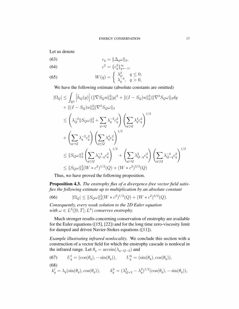
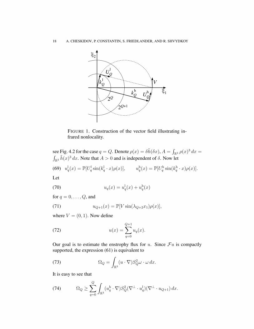
Example illustrating infrared nonlocality. We conclude this section with aconstruction of a vector field for which the enstrophy cascade is nonlocal inthe infrared range. Let θq = arcsin(λq−Q−2) and

(67) U lq = (cos(θq),− sin(θq)), Uh

q = (sin(θq), cos(θq)),

(68)kl

q = λq(sin(θq), cos(θq)), khq = (λ2

Q+2 − λ2q)

1/2(cos(θq),− sin(θq)),


ξ1

ξ2

2Q+1

2Q

V

UQ

kQ

h

kQ

l

l

hUQ

FIGURE 1. Construction of the vector field illustrating in-frared nonlocality.

see Fig. 4.2 for the case q = Q. Denote ρ(x) = δh(δx), A =∫R3 ρ(x)3 dx =∫

R3 h(x)3 dx. Note that A > 0 and is independent of δ. Now let

(69) ulq(x) = P[U l

q sin(klq · x)ρ(x)], uh

q (x) = P[Uhq sin(kh

q · x)ρ(x)].

Let

(70) uq(x) = ulq(x) + uh

q (x)

for q = 0, . . . , Q, and

(71) uQ+1(x) = P[V sin(λQ+2x1)ρ(x)],

where V = (0, 1). Now define

(72) u(x) =

Q+1∑q=0

uq(x).

Our goal is to estimate the enstrophy flux for u. Since Fu is compactlysupported, the expression (61) is equivalent to

(73) ΩQ =

∫

R3

(u · ∇)S2Qω · ω dx.

It is easy to see that

(74) ΩQ ≥Q∑

q=0

∫

R3

(uhq · ∇)S2

Q(∇⊥ · ulq)(∇⊥ · uQ+1) dx.


Using Lemma 3.6 we obtain

ΩQ ≥ A

Q∑q=0

|Uhq |λ2

q|U lq|λQ+2|V |+ O(δ)

= λQ+2‖∆Q+2u‖3

Q∑q=0

λ2q‖∆qu‖2

3 + O(δ),

(75)

which shows sharpness of (66) in the infrared range.

5. INEQUALITIES FOR THE NONLINEAR TERM

We take d = 3 and consider u, v ∈ B133,2 with ∇ · u = 0 and wish to

examine the advective term

(76) B(u, v) = P(u · ∇v) = ΛH(u⊗ v)

where

(77) [H(u⊗ v)]i = Rj(ujvi) + Ri(RkRl(ukvl))

and P is the Leray-Hodge projector, Λ = (−∆)12 is the Zygmund operator

and Rk = ∂kΛ−1 are Riesz transforms.

Proposition 5.1. The bilinear advective term B(u, v) maps continuously

the space B133,2 × B

133,2 to the space B

− 13

32,2

+ B− 2

395,2

. More precisely, there exist

bilinear continuous maps C(u, v), I(u, v) so that B(u, v) = C(u, v) +

I(u, v) and constants C such that, for all u, v ∈ B133,2 with ∇ · u = 0,

(78) ‖C(u, v)‖B− 1

332 ,2

≤ C‖u‖B

133,2

‖v‖B

133,2

and

(79) ‖I(u, v)‖B− 2

395 ,2

≤ C‖u‖B

133,2

‖v‖B

133,2

hold. If u, v, w ∈ B12187

,2then

(80) |〈B(u, v), w〉| ≤ C‖u‖B

12187 ,2

‖v‖B

12187 ,2

‖w‖B

12187 ,2

holds. So the trilinear map (u, v, w) 7→ 〈B(u, v), w〉 defined for smooth

vector fields in L3 has a unique continuous extension to

B12187

,2

3

and a

fortiori to

H56

3

.


Proof. We use duality. We take w smooth (w ∈ B2394,2

) and take the scalarproduct

〈B(u, v), w〉 =

∫

R3

B(u, v) · wdx

We write, in the spirit of the paraproduct of Bony ([1])

(81) ∆q(B(u, v)) = Cq(u, v) + Iq(u, v)

with

(82) Cq(u, v) =∑

p≥q−2, |p−p′|≤2

∆q(ΛH(∆pu, ∆p′v))

and(83)

Iq(u, v) =2∑

j=−2

[∆qΛH(Sq+j−2u, ∆q+jv) + ∆qΛH(Sq+j−2v, ∆q+ju)]

We estimate the contribution coming from the Cq(u, v):

∑q

|〈Cq(u, v), w〉|

≤ C∑

|q−q′|≤1

∑

p≥q−2, |p−p′|≤2

λqλ− 2

3p ‖Λ 1

3 ∆pu‖L3‖Λ 13 ∆p′v‖L3‖∆q′w‖L3

= C∑

|p−p′|≤2

λ− 2

3p ‖Λ 1

3 ∆pu‖L3‖Λ 13 ∆p′v‖L3

∑

q≤p+2,|q−q′|≤1

λ23q ‖Λ 1

3 ∆q′w‖L3

≤ C

∑

|p−p′|≤2

‖Λ 13 ∆pu‖ L3‖Λ 1

3 ∆p′v‖L3

‖w‖

B133,2

≤ C‖u‖B

133,2

‖v‖B

133,2

‖w‖B

133,2

.

This shows that the bilinear map C(u, v) =∑

q≥−1 Cq(u, v) maps continu-

ously

B133,2

2

to B− 1

332,2

and

(84) |〈C(u, v), w〉| ≤ C‖u‖B

133,2

‖v‖B

133,2

‖w‖B

133,2


The terms Iq(u, v) contribute

∑|〈Iq(u, v), w〉|

≤ C∑

|j|≤2, |q−q′|≤1

λq‖Sq+j−2u‖L92‖∆q+jv‖L3‖∆q′w‖L

94

+∑

|j|≤2, |q−q′|≤1

λq‖Sq+j−2v‖L92‖∆q+ju‖L3‖∆q′w‖L

94

≤ C‖u‖B

133,2

∑

|j|≤2,|q−q′|≤1

λ13q ‖∆q+jv‖L3λ

23q ‖∆q′w‖L

94

+C‖v‖B

133,2

∑

|j|≤2,|q−q′|≤1

λ13q ‖∆q+ju‖L3λ

23q ‖∆q′w‖L

94

≤ C‖u‖B

133,2

‖v‖B

133,2

‖w‖B

2394 ,2

Here we used the fact that

supq≥0

‖Squ‖L92≤ C‖u‖

B133,2

This last fact is proved easily:

‖Sq(u)‖L

92≤

∥∥∥∥∥∥

(∑j≤q

|∆ju|2) 1

2

∥∥∥∥∥∥L

92

≤∑

j≤q

‖∆ju‖2

L92

12

≤ C‖u‖B

133,2

We used Minkowski’s inequality in L94 in the penultimate inequality and

Bernstein’s inequality in the last. This proves that I maps continuouslyB

133,2 ×B

133,2 to B

− 23

95,2

.The proof of (80) follows along the same lines. Because of Bernstein’s

inequalities, the inequality (84) for the trilinear term 〈C(u, v), w〉 is stronger


than (80). The estimate of I follows:∑

|〈Iq(u, v), w〉|≤ C

∑

|j|≤2, |q−q′|≤1

λq‖Sq+j−2u‖L92‖∆q+jv‖L

187‖∆q′w‖L

187

+∑

|j|≤2, |q−q′|≤1

λq‖Sq+j−2v‖L92‖∆q+ju‖L

187‖∆q′w‖L

187

≤ C‖u‖B

133,2

∑

|j|≤2,|q−q′|≤1

λ12q ‖∆q+jv‖L

187λ

12q ‖∆q′w‖L

187

+C‖v‖B

133,2

∑

|j|≤2,|q−q′|≤1

λ12q ‖∆q+ju‖L

187λ

12q ‖∆q′w‖L

187

≤ C

[‖u‖

B133,2

‖v‖B

12187 ,2

+ ‖v‖B

133,2

‖u‖B

12187 ,2

]‖w‖

B12187 ,2

This concludes the proof. 2

The inequality (84) is not true for 〈B(u, v), w〉 and (80) is close to beingoptimal:

Proposition 5.2. For any 0 ≤ s ≤ 12, 1 < p < ∞, 2 < r ≤ ∞ there

exist functions u, v, w ∈ Bsp,r and smooth, rapidly decaying functions vn,

wn, such that limn→∞ vn = v, limn→∞ wn = w hold in the norm of Bsp,r

and such thatlim

n→∞〈B(u, vn), wn〉 = ∞

Proof. We start the construction with a divergence-free, smooth functionu such that Fu ∈ C∞

0 (B(0, 14)) and

∫u3

1dx > 0. We select a directione = (1, 0, 0) and set Φ = (0, u1, 0). Then

(85) A :=

∫

R3

(u(x) · e)∣∣P⊥

e Φ(x)∣∣2 dx > 0.

Next we consider the sequence aq = 1√q

so that (aq) ∈ `r(N) for r > 2, butnot for r = 2, and the functions

(86) vn =n∑

q=1

λ− 1

2q aqP [sin(λqe · x)Φ(x)]

and

(87) wn =n∑

q=1

λ− 1

2q aqP [cos(λqe · x)Φ(x)] .

Clearly, the limits v = limn→∞ vn and w = limn→∞ wn exist in norm inevery Bs

p,r with 0 ≤ s ≤ 12, 1 < p < ∞ and r > 2. Manifestly, by


construction, u, vn and wn are divergence-free, and because their Fouriertransforms are in C∞

0 , they are rapidly decaying functions. Clearly also

〈B(u, vn), wn〉 =

∫

R3

P(u · ∇vn)wndx =

∫

R3

(u · ∇vn) · wndx.

The terms corresponding to each q in

(88)

u · ∇vn =n∑

q=1

(u(x) · e)aqλ− 1

2q P [cos(λqe · x)Φ(x)]

+n∑

q=1

aqλ− 1

2q u(x) · P [sin(λqe · x)∇Φ(x)]

and in (87) have Fourier transforms supported on B(λqe,12) ∪ B(−λqe,

12).

These are mutually disjoint sets for distinct q and, consequently, the termscorresponding to different indices q do not contribute to the integral

∫(u ·

∇vn) · wndx. The terms from the second sum in (88) form a convergentseries. Therefore, using Lemma 3.6, we obtain∫

R3

(u · vn) · wn =n∑

q=1

a2q

∫

R3

(u(x) · e) P [cos(λqe · x)Φ(x)]2 dx + O(1)

=n∑

q=1

a2q

∫

R3

(u(x) · e)∣∣P⊥

e Φ(x)∣∣2 dx + O(1)

=

[n∑

q=1

a2q

]A + O(1),

which concludes the proof. ¤

6. REMARKS

In [13], Duchon and Robert have shown that a weak solution u to the 3DEuler or 3D Navier-Stokes equations conserves energy provided

(89)∫|u(x, t)− u(x− y, t)|3 dx = C(t)|y|σ(|y|), ∀y ∈ R3,

for some C(t) integrable on [0, T ] and σ(a), such that σ(a) → 0 as a → 0.

Here we show that there are functions in L3((0, T ); B133,p(R3)), p > 1 that

do not satisfy (89). Namely, any function on [0, T ] of the form

u(x, t) = (sin(λ(t)x1)ρ(x), 0, 0),

where ρ = F−1(χ(4·)) and λ(t) is integrable, belongs to L3((0, T ); B133,p)

for all p > 1. However, u does not satisfy Duchon-Robert condition (89)


provided λ(t)3 is not integrable. Indeed, suppose that (89) is satisfied. Thenfor |y| ¿ 1 and λ ≤ |y|−1 we have

C(t)|y|σ(|y|) =

∫|u(x)− u(x− y)|3 dx ∼ λ3|y|3.

Let us fix t0, such that C(t0) > 0. Then for |y| small enough with |y| ≤λ−1(t0) we have

(90) C(t0)σ(|y|) ∼ λ(t0)3|y|2.

Now, for every t with λ(t) À 1 we set |y| = λ(t)−1 and obtain

C(t)λ(t)−1σ(λ(t)−1) ∼ 1.

Hence, using (90) we obtain

C(t) ∼ λ(t)σ(λ(t)−1)−1 ∼ λ(t)3C(t0)λ(t0)−3,

which is not integrable, a contradiction.We also note that the estimates on the energy flux in Section 3.2 can be

applied to weak solutions of the 3D Navier-Stokes equations.

Theorem 6.1. Let u ∈ L∞((0, T ); L2(R3))∩L2((0, T ); H1(R3)) be a weaksolution to the 3D incompressible Navier-Stokes equations with

u ∈ L3((0, T ); B133,∞).

Then u satisfies energy equality, i.e., ‖u(t)‖22 is absolutely continuous on

[0, T ].

Hence the techniques in this present paper give stronger results than thosein [13] for the conditions under which it can be proved that the energy bal-ance equation holds for the both the Euler and the Navier-Stokes equations.

ACKNOWLEDGMENT

The work of AC was partially supported by NSF PHY grant 0555324,the work of PC by NSF DMS grant 0504213, the work of SF by NSF DMSgrant 0503768, and the work of RS by NSF DMS grant 0604050. Theauthors also would like to thank the referee for many helpful suggestions.

REFERENCES

[1] J-M Bony, Calcul symbolique et propagation des singularite pour lesequations auxderivees partielles non lineaires, Ann. Ecole Norm. Sup. 14 (1981) 209–246.

[2] D. Chae, Remarks on the helicity of the 3-D incompressible Euler equations, Comm.Math. Phys. 240 (2003), 501–507.

[3] J-Y Chemin, Perfect Incompressible Fluids, Clarendon Press, Oxford Univ 1998.[4] J-Y Chemin and N. Masmoudi. About lifespan of regular solutions of equations re-

lated to viscoelastic fluids. SIAM J. Math. Anal., 33 (electronic), (2001), 84-112.


[5] A. Cheskidov, S. Friedlander and N. Pavlovic, An inviscid dyadic model of turbu-lence: the fixed point and Onsager’s conjecture, Journal of Mathematical Physics, toappear.

[6] A. Cheskidov, S. Friedlander and N. Pavlovic, An inviscid dyadic model of turbu-lence: the global attractor (with S. Friedlander and N. Pavlovic), preprint.

[7] P. Constantin, The Littlewood-Paley spectrum in 2D turbulence, Theor. Comp. FluidDyn.9 (1997), 183-189.

[8] P. Constantin and N Masmoudi, Global well-posedness for a Smoluchowski equationcoupled with Navier-Stokes equations in 2D, preprint, math.AP/0702589.

[9] P. Constantin, W. E, E. Titi, Onsager’s conjecture on the energy conservation forsolutions of Euler’s equation, Commun. Math. Phys. 165 (1994), 207–209.

[10] P. Constantin, B. Levant, E. Titi, Regularity of inviscid shell models of turbulence,Physical Review E 75 1 (2007) 016305.

[11] P. Constantin, F. Ramos, Inviscid limit for damped and driven incompressible Navier-Stokes equations in R2, Commun. Math. Phys., to appear (2007).

[12] C. De Lellis and L. Szekelyhidi, The Euler equations as differential inclusion,preprint.

[13] J. Duchon and R. Robert, Inertial energy dissipation for weak solutions of incom-pressible Euler and Navier-Stokes equations, Nonlinearity 13 (2000), 249–255.

[14] G. L. Eyink, Energy dissipation without viscosity in ideal hydrodynamics. I. Fourieranalysis and local energy transfer, Phys. D 78 (1994), 222–240.

[15] G. L. Eyink, Locality of turbulent cascades, Phys. D 207 (2005), 91–116.[16] G. L. Eyink and K. R. Sreenivasan, Onsager and the theory of hydrodynamic turbu-

lence, Rev. Mod. Phys. 78 (2006).[17] U. Frisch, Turbulence. The legacy of A. N. Kolmogorov. Cambridge University Press,

Cambridge, 1995.[18] A. N. Kolmogorov, The local structure of turbulence in incompressible viscous fluids

at very large Reynolds numbers, Dokl. Akad. Nauk. SSSR 30 (1941), 301–305.[19] R. H. Kraichnan, The structure of isotropic turbulence at very high Reynolds num-

bers, J. Fluid Mech. 5 (1959), 497–543.[20] R. H. Kraichnan, Inertial ranges in two-dimensional turbulence, Phys. Fluids 10

(1967), 1417-1423.[21] P-G Lemarie-Rieusset, Recent developments in the Navier-Stokes problem, Chapman

and Hall/CRC, Boca Raton, 2002.[22] M. Lopes Filho, A. Mazzucato, H. Nussenzveig-Lopes, Weak solutions, renormalized

solutions and enstrophy defects in 2D turbulence, ARMA 179 (2006), 353-387.[23] H. K. Moffatt and A. Tsinober, Helicity in laminar and turbulent flow, Ann. Rev. Fluid

Mech. 24 (1992), 281–312.[24] L. Onsager, Statistical Hydrodynamics, Nuovo Cimento (Supplemento) 6 (1949),

279–287.[25] R. Robert, Statistical Hydrodynamics ( Onsager revisited ), Handbook of Mathemat-

ical Fluid Dynamics, vol 2 ( 2003), 1–55. Ed. Friedlander and Serre. Elsevier.[26] V. Scheffer, An inviscid flow with compact support in space-time, J. Geom. Anal.

3(4) (1993), 343–401.[27] A. Shnirelman, On the nonuniqueness of weak solution of the Euler equation, Comm.

Pure Appl. Math. 50 (1997), 1261–1286.


(A. Cheskidov and P. Constantin) DEPARTMENT OF MATHEMATICS, UNIVERSITY OFCHICAGO, CHICAGO, IL 60637

E-mail address: [email protected] address: [email protected]

(S. Friedlander and R. Shvydkoy) DEPARTMENT OF MATHEMATICS, STAT. ANDCOMP. SCI., UNIVERSITY OF ILLINOIS, CHICAGO, IL 60607

E-mail address: [email protected]

E-mail address: [email protected]

Date post:	25-Apr-2018
Category:	Documents
Upload:	trinhdien
View:	216 times
Download:	2 times

ENERGY CONSERVATION AND ONSAGER’S ...homepages.math.uic.edu/~shvydkoy/papers/onsager.pdfENERGY...

Documents