Energy Consumption in Mobile Phones: A Measurement Study and Implications for Network Applications Niranjan Balasubramanian Aruna Balasubramanian Arun Venkataramani Department of Computer Science University of Massachusetts Amherst {niranjan, arunab, arun}@cs.umass.edu ABSTRACT In this paper, we present a measurement study of the energy con- sumption characteristics of three widespread mobile networking technologies: 3G, GSM, and WiFi. We find that 3G and GSM in- cur a high tail energy overhead because of lingering in high power states after completing a transfer. Based on these measurements, we develop a model for the energy consumed by network activity for each technology. Using this model, we develop TailEnder, a protocol that reduces energy consumption of common mobile applications. For appli- cations that can tolerate a small delay such as e-mail, TailEnder schedules transfers so as to minimize the cumulative energy con- sumed while meeting user-specified deadlines. We show that the TailEnder scheduling algorithm is within a factor 2× of the optimal and show that any online algorithm can at best be within a factor 1.62× of the optimal. For applications like web search that can benefit from prefetching, TailEnder aggressively prefetches several times more data and improves user-specified response times while consuming less energy. We evaluate the benefits of TailEnder for three different case study applications—email, news feeds, and web search—based on real user logs and show significant reduction in energy consumption in each case. Experiments conducted on the mobile phone show that TailEnder can download 60% more news feed updates and download search results for more than 50% of web queries, compared to using the default policy. Categories and Subject Descriptors C.2 [Computer Communication Network]: Network Architec- ture and Design— Wireless Communication General Terms Algorithms, Design, Performance Keywords Cellular networks, WiFi, Power measurement, Energy savings, Mo- bile applications Permission to make digital or hard copies of all or part of this work for personal or classroom use is granted without fee provided that copies are not made or distributed for profit or commercial advantage and that copies bear this notice and the full citation on the first page. To copy otherwise, to republish, to post on servers or to redistribute to lists, requires prior specific permission and/or a fee. IMC’09, November 4–6, 2009, Chicago, Illinois, USA. Copyright 2009 ACM 978-1-60558-770-7/09/11 ...$10.00. 1. INTRODUCTION Mobile phones are ubiquitous today with an estimated cellular subscription of over 4 billion worldwide [2]. Most phones today support one or more of 3G, GSM, and WiFi for data transfer. For example, the penetration of 3G is estimated at over 15% of cellular subscriptions worldwide and is over 70% in some countries [1]. How do the energy consumption characteristics of network ac- tivity over 3G, GSM, and WiFi on mobile phones compare with each other? How can we reduce the energy consumed by common applications using each of these three technologies? To investigate these questions, we first conduct a detailed measurement study to quantify the energy consumed by data transfers across 3G, GSM, and WiFi. We find that the energy consumption is intimately re- lated to the characteristics of the workload and not just the total transfer size, e.g., a few hundred bytes transferred intermittently on 3G can consume more energy than transferring a megabyte in one shot. Below is a summary of the key findings of our measurement study, which remain consistent across three different cities, diurnal variation, mobility patterns, and devices. 1. In 3G, a large fraction (nearly 60%) of the energy, referred to as the tail energy, is wasted in high-power states after the completion of a transfer. In comparison, the ramp energy spent in switching to this high-power state before the transfer is small. Tail and ramp energies are constants that amortize over larger transfer sizes or frequent successive transfers. 2. In GSM, although a similar trend exists, the time spent in the high-power state after the transfer, or the tail time, is much smaller compared to 3G (6 vs. 12 secs). Furthermore, the lower data rate of GSM implies that more energy is spent in the actual transfer of data. 3. In WiFi, the association overhead is comparable to the tail energy of 3G, but the data transfer itself is significantly more efficient than 3G for all transfer sizes. Based on these findings, we develop a simple model of energy consumption of network activity for each of the three technolo- gies. We utilize these models to identify opportunities for reducing the energy consumption of network activity induced by common mobile applications. To this end, we design TailEnder, an energy- efficient protocol for scheduling data transfers. TailEnder considers two classes of applications: 1) delay-tolerant applications such as email and RSS feeds, and 2) applications such as web search and web browsing that can benefit from aggressive prefetching. For delay-tolerant applications on 3G and GSM, TailEnder sched- ules outgoing transfers so as to minimize the overall time spent in high energy states after completing transfers, while respecting user- specified delay-tolerance deadlines. We show that the TailEnder
Transcript
Energy Consumption in Mobile Phones: A MeasurementStudy and Implications for Network Applications
Niranjan Balasubramanian Aruna Balasubramanian Arun VenkataramaniDepartment of Computer Science
University of Massachusetts Amherst{niranjan, arunab, arun}@cs.umass.edu
ABSTRACTIn this paper, we present a measurement study of the energy con-sumption characteristics of three widespread mobile networkingtechnologies: 3G, GSM, and WiFi. We find that 3G and GSM in-cur a high tail energy overhead because of lingering in high powerstates after completing a transfer. Based on these measurements,we develop a model for the energy consumed by network activityfor each technology.
Using this model, we develop TailEnder, a protocol that reducesenergy consumption of common mobile applications. For appli-cations that can tolerate a small delay such as e-mail, TailEnderschedules transfers so as to minimize the cumulative energy con-sumed while meeting user-specified deadlines. We show that theTailEnder scheduling algorithm is within a factor 2× of the optimaland show that any online algorithm can at best be within a factor1.62× of the optimal. For applications like web search that canbenefit from prefetching, TailEnder aggressively prefetches severaltimes more data and improves user-specified response times whileconsuming less energy. We evaluate the benefits of TailEnder forthree different case study applications—email, news feeds, and websearch—based on real user logs and show significant reduction inenergy consumption in each case. Experiments conducted on themobile phone show that TailEnder can download 60% more newsfeed updates and download search results for more than 50% ofweb queries, compared to using the default policy.
Categories and Subject DescriptorsC.2 [Computer Communication Network]: Network Architec-ture and Design— Wireless Communication
General TermsAlgorithms, Design, Performance
KeywordsCellular networks, WiFi, Power measurement, Energy savings, Mo-bile applications
Permission to make digital or hard copies of all or part of this work forpersonal or classroom use is granted without fee provided that copies arenot made or distributed for profit or commercial advantage and that copiesbear this notice and the full citation on the first page. To copy otherwise, torepublish, to post on servers or to redistribute to lists, requires prior specificpermission and/or a fee.IMC’09, November 4–6, 2009, Chicago, Illinois, USA.Copyright 2009 ACM 978-1-60558-770-7/09/11 ...$10.00.
1. INTRODUCTIONMobile phones are ubiquitous today with an estimated cellular
subscription of over 4 billion worldwide [2]. Most phones todaysupport one or more of 3G, GSM, and WiFi for data transfer. Forexample, the penetration of 3G is estimated at over 15% of cellularsubscriptions worldwide and is over 70% in some countries [1].
How do the energy consumption characteristics of network ac-tivity over 3G, GSM, and WiFi on mobile phones compare witheach other? How can we reduce the energy consumed by commonapplications using each of these three technologies? To investigatethese questions, we first conduct a detailed measurement study toquantify the energy consumed by data transfers across 3G, GSM,and WiFi. We find that the energy consumption is intimately re-lated to the characteristics of the workload and not just the totaltransfer size, e.g., a few hundred bytes transferred intermittently on3G can consume more energy than transferring a megabyte in oneshot. Below is a summary of the key findings of our measurementstudy, which remain consistent across three different cities, diurnalvariation, mobility patterns, and devices.
1. In 3G, a large fraction (nearly 60%) of the energy, referredto as the tail energy, is wasted in high-power states after thecompletion of a transfer. In comparison, the ramp energyspent in switching to this high-power state before the transferis small. Tail and ramp energies are constants that amortizeover larger transfer sizes or frequent successive transfers.
2. In GSM, although a similar trend exists, the time spent in thehigh-power state after the transfer, or the tail time, is muchsmaller compared to 3G (6 vs. 12 secs). Furthermore, thelower data rate of GSM implies that more energy is spent inthe actual transfer of data.
3. In WiFi, the association overhead is comparable to the tailenergy of 3G, but the data transfer itself is significantly moreefficient than 3G for all transfer sizes.
Based on these findings, we develop a simple model of energyconsumption of network activity for each of the three technolo-gies. We utilize these models to identify opportunities for reducingthe energy consumption of network activity induced by commonmobile applications. To this end, we design TailEnder, an energy-efficient protocol for scheduling data transfers. TailEnder considerstwo classes of applications: 1) delay-tolerant applications such asemail and RSS feeds, and 2) applications such as web search andweb browsing that can benefit from aggressive prefetching.
For delay-tolerant applications on 3G and GSM, TailEnder sched-ules outgoing transfers so as to minimize the overall time spent inhigh energy states after completing transfers, while respecting user-specified delay-tolerance deadlines. We show that the TailEnder
scheduling algorithm is provably within a factor 2× of the energyconsumed by an optimal offline algorithm that knows the completearrival pattern of transfers a priori. Furthermore, we show that nodeterministic online algorithm can be better than 1.62-competitivewith respect to an optimal offline adversary.
For applications that can benefit from prefetching, TailEnder de-termines what data to prefetch so as to minimize the overall energyconsumed. Prefetching useful data reduces the number of trans-fers and their associated cumulative tail energy, while prefetch-ing useless data incurs additional transmission energy. TailEnderuses a probabilistic strategy to balance these concerns. Somewhatcounterintuitively, for applications such as web search, TailEnderfetches several times more data and improves user-perceived re-sponse times, but still consumes less energy.
We evaluate the performance of TailEnder for three different ap-plications: email, news feeds and web search. For each of theseapplications, we collect real user traces including arrival times andtransfer sizes. We evaluate TailEnder by conducting experimentson the mobile phone and find that TailEnder can download 60%more news feed updates and download search results for more than50% of web queries, compared to using the default policy. Ourmodel-driven simulation shows that TailEnder can reduce energyby 35% for email applications, 52% for news feeds and 40% forweb search. Further, we find that, opportunistic WiFi access sub-stantially reduces energy consumption compared to only using 3G.Even when WiFi in only available 50% of the time, sending dataover WiFi when available reduces the energy consumption by over3 times for all three applications.
2. BACKGROUND AND RELATED WORK
2.1 Cellular power managementTwo factors determine the energy consumption due to network
activity in a cellular device. First, is the transmission energy that isproportional to the length of a transmission and the transmit powerlevel. Second, is the Radio Resource Control (RRC) protocol that isresponsible for channel allocation and scaling the power consumedby the radio based on inactivity timers.
IDLEDCH
FACH
NOT CONNECTEDCONNECTED
POWER
(a) (b)
Figure 1: (a) The radio resource control state machine for3GPP networks consisting of three states: IDLE, DCH andFACH (b) Instantaneous power measurements for an exampletransfer over 3G showing the transition time between high tolow power state
Figure 1(a) shows the state machine [18] implemented by theRRC protocol for GSM/EDGE/GPRS (2.5G) as well as UMTS/WCDMA(3G) networks that follow the 3GPP [5] standard. The radio re-mains in the IDLE state in the absence of any network activity. The
radio transitions to the higher power states, DCH (Dedicated Chan-nel) or FACH (Forward Access Channel), when the network is ac-tive. The DCH state reserves a dedicated channel to the deviceand ensures high throughput and low delay for transmissions, butat the cost of high power consumption. The FACH state shares thechannel with other devices and is used when there is little traffic totransmit and consumes about half of the power in the DCH state.The IDLE state consumes about one percent of the power in theDCH state.
The transition between the different states is controlled by in-activity timers [18]. Figure 1(b) shows the instantaneous powermeasurements for an example transfer. The graph shows the timetaken to transition from a high power to a low power state. Insteadof transitioning from the high to the low power state immediatelyafter a packet is transmitted, the device transitions only when thenetwork has been inactive for the length of the inactivity timer. Thismechanism serves two benefits: 1) it alleviates the delay incurredin moving to the high power state from the idle state, and 2) it re-duces the signaling overhead incurred due to channel allocation andrelease during state transitions. Since lingering in the high powerstate also consumes more energy, network operators set the value ofthe inactivity timer based on this peformance/energy trade-off [18,12], with typical values being several seconds long.
The 3GPP2 standard [4] used by the CDMA2000 technology isanother standard for 3G networks, and 3GPP and 3GPP2 are themost prevalent standards today. Though the state machine for theradio resource control in the 3GPP2 standard is different from thatshown in Figure 1, several features are similar. In particular, the3GPP2 standard also uses an inactivity timer to transition from thehigh power to the low power state for performance reasons [18, 25].
2.2 WiFi power managementIn comparison, WiFi incurs a high initial cost of associating with
an access point (AP). However, because WiFi on phones typicallyuses the Power Save Mode (PSM), the cost of maintaining the as-sociation is small. When associated, the energy consumed by adata transfer is proportional to the size of the data transfer and thetransmit power level. Our measurements (Section 3) confirm thatthe transmission energy consumed by WiFi is significantly smallerthan both 3G and GSM, especially for large transfer sizes.
2.3 Related workEnergy consumption of network activity in mobile phones has
seen a large body of work in recent times. To our knowledge, ourpaper presents the first comparative study of energy consumptioncharacteristics of all three technologies—3G, GSM, and WiFi—that are under widespread use today. In particular, our study of theenergy consumption characteristics of 3G reveals significant andnonintuitive implications for energy-efficient application design.
Analytical modeling. Prior work [18, 25, 12] has studiedthe impact of different energy saving techniques in 3G networksusing analytical models. These works analyze the impact of theinactivity timer by modeling the delay and energy utilization fordifferent values for the inactivity timer. Their goal is to determinethe optimal value of the inactivity timer from the network opera-tor’s perspective. Yeh et al. [25] analytically compare the impactof the inactivity timer in both 3GPP and 3GPP2 networks. In com-parison, our study treats the inactivity timer value as a given anddevelops algorithms for energy-efficient application design basedon real measurements and application traces.
Measurement. Gupta et al. [14] present a measurement studyof the energy consumption of VoIP applications over WiFi-basedmobile phones. The authors find that intelligent scanning strategies
and aggressive use of PSM in WiFi can reduce power consump-tion for VoIP applications. Xiao et al. [24] measure the energyconsumption for Youtube-like video streaming applications in mo-bile phones using both WiFi and 3G. Their focus is on the energyutilization of various storage strategies and application-level strate-gies such as delayed-playback and playback after download. Nur-minen et al. [20] measure the energy consumption for peer-to-peerapplications over 3G. In comparison to these application-specificstudies, our focus is on reducing the energy consumption of gen-eral network activity across 3G, GSM, and WiFi.
Energy-efficient mobile network activity. Several previ-ous studies [6, 22, 23, 7] have investigated strategies for energy-efficient network activity in mobile phones supporting multiple wire-less technologies. Pering et al. [22] develop strategies to intelli-gently switch between WiFi and Bluetooth. Agarwal et al. [6] pro-pose an architecture to use the GSM radio to wake up the WiFiradio upon an incoming VoIP call to leverage the better qualityand energy-efficiency of WiFi while keeping its scanning costs low.Krashinsky et al. [17] present an alternative to the 802.11 powersaving mode to minimize energy consumption over WiFi. The au-thors present an adaptive algorithm that minimizes energy by deter-mining the length of time that the WiFi interface should be switchedoff based on network activity without affecting performance.
Rahmati et al. [23] show that intelligently switching betweenWiFi and GSM reduces energy consumption substantially as WiFiconsumes less transmission power. However, in order to avoid thecost of unnecessary scanning in the face of poor WiFi availability,the authors design an algorithm that predicts WiFi availability, andthe device scans for WiFi access points only in areas where WiFi isavailable with high probability. Trevor et al. [7] present application-level modifications to reduce energy consumption for updates todynamic web content. Their key ideas include using a proxy to 1)only push new content when the portion of the web document of in-terest to the user is updated, 2) batch updates to avoid the overheadof repeated polling, and 3) use SMS on GSM to signal the selec-tion of WiFi or GSM based on the transfer size for energy-efficientdata transfer. In addition to confirming these prior findings aboutGSM and WiFi power consumption, our measurement study alsoinvestigates 3G that reveals significantly different energy consump-tion characteristics, which lead us to develop novel energy-efficientdata transfer algorithms for 3G.
Algorithms. Prior theoretical works [11, 13, 15, 8] studythe problem of energy minimization while meeting job deadlinesin processors that transition between the sleep and active state. Themodel assumed in most of these works is that a device incurs a largeramp energy overhead in transitioning from the low power state tothe high power state, so the goal is to minimize the number of tran-sitions. As explained in Sections 3 and 4, this model cannot beapplied as is to mobile phones because their transition characteris-tics are different and include a significant tail energy component.
3. MEASUREMENTWe conduct a measurement study with the following goals:
1. Compare the energy consumption characteristics of 3G, GSMand WiFi and measure the fraction of energy consumed fordata transfer versus overhead.
2. Analyze the variation of the energy overhead with geographiclocation, time-of-day, mobility, and devices.
3. Develop a simple energy model to quantify the energy con-sumption over 3G, WiFi and GSM as a function of the trans-fer size and the inter-transfer times.
0
2
4
6
8
10
12
14
Transfer Ramp Tail
Energy(Joules)
Components Total
(a) 3G: Energy components
0
5
10
15
20
25
1 2 3 4 5 6 7 8 9 10111213141516171819
Energy(Joules)
Timebetweentransfers(seconds)
1K 5K 10K 50K 100K 500K
(b) 3G: Varying inter-transfer times
Figure 2: 3G Measurements: (a) Average ramp, transfer andtail energy consumed to download 50K data. The lower por-tion of the stacked columns show the proportion of energy spentfor each activity compared to the total energy spent. (b) Aver-age energy consumed for downloading data of different sizesagainst the inter-transfer time
3.1 Devices and ToolsThe majority of our experiments are performed using four Nokia
N95 phones (http://en.wikipedia.org/wiki/Nokia_N95). Two of thephones are 3G-enabled AT&T phones that use HSDPA/UMTS tech-nology and two are GSM-enabled AT&T phones that use EDGE.All four phones were equipped with an 802.11b WiFi interface. Weuse Python, PyS60 v1.4.2, developed for the Symbian OS 3rdEdFP 1 to conduct data transfer experiments. To measure energy con-sumption, we use Nokia’s energy profiling application, the NokiaEnergy Profiler (NEP) v1.1 1. NEP provides instantaneous powermeasurements sampled once every 250 milli-seconds. Using thepower measurements, we estimate the energy consumed by approx-imating the area under the power measurement curve over a timeinterval. Unless stated, all measurement results are averaged over20 trials and error bars show the 95% confidence interval.
We also report results from a smaller scale measurement studyperformed on the HTC Fuze phone that runs Windows Mobile 6.5.The HTC phone is also a 3G-enabled AT&T phone and is equippedwith an 802.11b WiFi interface.The energy measurements on theHTC phone were performed using a hardware power meter [3] thatmeasured power once every 0.2 milliseconds.
3.2.1 3G and GSMOur 3G and GSM measurements quantify the: 1) Ramp energy:
energy required to switch to the high-power state, 2) Transmissionenergy, and 3) Tail energy: energy spent in high-power state afterthe completion of the transfer.
We conduct measurements for data transfers of different sizes(1 to 1000 KB) with varying intervals (1 to 20 seconds) betweensuccessive transfers. We measure energy consumption by runningNEP in the background while making data transfers. For each con-figuration of (x, t), where x ∈ [1K, 1000K] and t ∈ [1, 20] sec-onds, the data transfers proceed as follows: The phone initiates anx KB upload/download by issuing a http-request to a remote server.After the upload/download is completed, the phone waits for t sec-onds and then issues the next http request. This process is repeated20 times for each data size. Between data transfer experiments fordifferent intervals, the phone remains idle for 60 seconds. The en-ergy spent during this period is subtracted from the measurementsas idle energy. We extract the energy measurements from the pro-filer for analysis, and use the time-stamps recorded by NEP to markthe beginning and end of data transfer as well as the beginning andend of the Ramp time and the tail-time. The energy consumed byeach data transfer is computed as the area under the power-curvebetween the end of Ramp time and the start of tail-time.
3.2.2 WiFiOur WiFi measurements quantify the energy : 1) to scan and
associate to an access point and 2) to transfer data. We conducttwo sets of measurements. In the first set of measurements, foreach data transfer, we first scan for WiFi access points, associatewith an available AP and then make the transfer. In the second setof measurements, we only make one scan and association for theentire set of data transfers to isolate the transfer energies.
In addition, all three networks, 3G, GSM and WiFi, incur a main-tenance energy, which is the energy used to keep the interface up.We estimate the maintenance energy per second by measuring thetotal energy consumed to keep the interface up for a time period.
3.2.3 Accounting for idle powerFor all measurements, we configure the phone in the lowest power
mode and turn off the display and all unused network interfaces.The energy profiler itself consumes a small amount of energy, whichwe include in the idle power measurement. We measure idle energyby letting the energy profiler run in the background with no otherapplication activity. The average idle power is less than 0.05 W andrunning the energy profiler at a sampling frequency of 0.25 secondsincreases the power to 0.1 W.
3.3 3G MeasurementsFigure 2(a) shows the average energy consumption for a typical
50KB download over 3G. We find that the Tail energy is more than60% of the total energy. The Ramp energy is significantly smallcompared to the tail energy, and is only 14% of the total energy.3G also incurs a maintenance energy to keep the interface on, andis between 1-2 Joules/minute (not shown).
Figure 2(b) shows the average energy consumed for downloadwhen the time between successive transfers is varied. We ignore theidle energy consumed when waiting to download the next packet.Consider the data points for downloading 100 KB data. The energyincreases from 5 Joules to 13 Joules as the time between successivedownloads increases from 1 second to 12 seconds. When the timebetween successive downloads is greater than 12.5 seconds, the en-
ergy consumed for 100 KB transfers plateaus at 15 Joules. Whenthe device waits less than the tail-time to send the next packet, eachdata transfer does not incur the total Tail energy penalty, reducingthe average energy per transfer. This observation suggests that theTail energy can be amortized using multiple transfers, but only ifthe transfers occur within tail-time of each other. This observationis crucial to the design of TailEnder, a protocol that reduces the en-ergy consumed by network applications running on mobile phones.
3.3.1 Geographical and Temporal variationsWe measure the energy consumption across different days and
in different geographical regions. The objectives of the experimentare 1) to verify that mobile phones in different cell tower areas areaffected by the tail-time overhead, and 2) to measure the temporalconsistency of tail-time.
Figure 3(a) shows that the Tail energy remains consistent acrossthree days. On the other hand, Figure 3(b) shows that the Rampenergy is about 2 and 4 Joules for the measurements conducted ondifferent days.
We conducted 3G energy measurements in three different cities,Amherst, Northamption and Boston, in Massachusetts, USA usingtwo different devices. Figure 3(c) shows that the Tail energy is con-sistent across different locations and two different Nokia devices(D1 and D2). The figure also shows that the Tail energy and Rampenergy do not vary across day (9:00 am to 5:00 pm) and night (8:00pm to 6:00 am). The measurement results provide additional ev-idence that the tail-time or the inactivity timer is configured stati-cally by network operators and can be inferred empirically. In Sec-tion 4, we use the value of the inactivity timer to design TailEnder.
Figure 4(a) compares the average energy consumed by down-loads during the day versus night, averaged over 3 days of transferdata. Although the ramp and tail energies are similar during nightand day (shown in Figure 3(c)), the energy consumed during thenight is up to 10% lower than during the day. This is likely due tolower congestion during the night.
3.3.2 UploadsFigure 4(b) shows the average tail, ramp and transfer energy for
upload experiments. As observed in the download experiments,the Tail energy consumes more than 55% of the total energy. Fig-ure 4(c) shows that the transfer energy for uploads is higher thandownloads for larger data sizes. For example, the transfer energyfor uploads is nearly 30% more than that for downloads for 100 KBtransfers. One cause for this difference is that upload bandwidthsare typically smaller than the download bandwidth.
3.3.3 MobilityFigure 5 compares energy consumption under mobility within
the town of Amherst, MA for 50K data transfers. Mobility inoutdoor settings affect transfer rates due to factors such as signalstrength and hand-offs between cell towers, resulting in varyingtransfer times [19]. Despite the large variances in the transfer en-ergy compared to the stationary measurements, we observe that theTail energy accounts for nearly 50% of the total energy even in themobile scenario.
3.4 GSM MeasurementsWe conducted a set of measurements using the two Nokia phones
equipped with GSM. Figure 6(a) shows the average energy con-sumption in GSM networks as a proportion of the Tail energy, Rampenergy and transfer energy for a 50K download. Unlike in 3G, theTail energy only accounts for 30% of the transfer energy. How-ever, similar to 3G, the Ramp energy in GSM is small compared to
0
5
10
15
20
0 10 20 30 40 50 60 70 80
Ene
rgy (
Joule
s)
Trial number
23-April27-April28-April
(a) Temporal variation: Tail energy
0
2
4
6
8
10
0 10 20 30 40 50 60 70 80
Ene
rgy (
Joule
s)
Trial number
23-April27-April28-April
(b) Temporal variation: Ramp energy
0
2
4
6
8
10
12
14
Energ
y (
Joule
s)
Amherst, D1Amherst, D2
Northampton, D2Boston, D1
Night, D1
(c) Geographical variation
Figure 3: 3G Measurements: 50K downloads (a) Tail energy over 3 days (b) Ramp energy over 3 days (c) Average tail and rampenergies measured in three cities using two devices D1 and D2.
0
5
10
15
20
25
1 10 100 1000
Energy(Joules)
DataSizeinKB
Day
Night
(a) Download: Day versus Night
0
5
10
15
20
Transfer Ramp Tail
Energy(Joules)
Components Total
(b) Upload measurements
0
5
10
15
20
1 10 100
Energy(Joules)
DataSizeinKB
Upload
Download
(c) Upload versus Download
Figure 4: 3G Measurements: (a) Comparison of average energy consumption of day versus night time downloads of 50K data.(b) Av-erage transfer, tail and ramp energy consumed for uploading 50K data (c) Comparing the average energy consumed for downloading50K data versus uploading 50K data.
0
5
10
15
20
25
30
Total Transfer Ramp Tail
Energy(Joules)
Stationary Mobile
Figure 5: 3G measurements with mobility: Average energy con-sumed for downloading 50K of data.
the Tail energy and the transfer energy. We also observed that thetail-time is 6 seconds and GSM incurs a small maintenance energybetween 2-3 J/minute (not shown in figure).
Due to the small tail-time in GSM (unlike 3G), data sizes dom-inate energy consumption rather than the inter-transfer times. Fig-ure 6(b) shows the average energy consumed when varying the timebetween successive transfers. The average energy does not varywith increasing inter-transfer interval. For example, for data trans-fers of size 100 KB, the average energy consumption is between 19
to 21 Joules even as the time between successive transfers varies. Incomparison, Figure 2(b) shows that the average energy consump-tion varies significantly in 3G with varying inter-transfer interval,until the inter-transfer interval grows to more than the tail-time.
3.5 WiFi MeasurementsFigure 7(a) shows the average energy consumption in WiFi com-
posed of scanning, association and transfer, for a 50 K download.We observe that the scanning and association energy is nearly fivetimes the transfer energy. Our results confirm previous measure-ments by Rahmati et al. [23].
Figure 7(b) shows that the energy consumption of WiFi increaseswith the time between successive transfers. Interestingly, the en-ergy consumption does not plateau after a threshold inter-transfertime like in 3G (Figure 2(b)). The reason for this monotonic in-crease is the high maintenance energy in WiFi. We measured themaintenance overhead (not shown) for keeping the WiFi interfaceon to be 3-3.5 Joules per minute.
3.6 3G vs GSM vs WiFiFigure 8 compares the average energy consumption of 3G, GSM
and WiFi. 3G consumes significantly more energy to downloaddata of all sizes (12-20J) compared to GSM and WiFi. GSM con-sumes 40% to 70% less energy compared to 3G. This is due to tworeasons – (1) GSM radios typically operate at a lower power level
Figure 6: GSM Measurements: (a) Average ramp, transferand tail energy consumed to download 50K data. The lowerportion of the stacked columns show the proportion of energyspent for each activity compared to the total energy spent. (b)Average energy consumed for downloading data of differentsizes against the inter-transfer time.
than 3G radios and (2) the Tail energy set for GSM is around 6 sec-onds, much lower than the 12.5 seconds set for 3G.
WiFi is more energy efficient than both cellular networks once itis connected to an access point (AP). Figure 8 shows that the trans-fer energy for WiFi grows nearly three times slower compared tothe cellular networks. For a download of size 10K, WiFi consumesone-sixth of 3G’s energy and one-third of GSM’s energy. With in-creasing data sizes WiFi’s efficiency increases dramatically. Thegraph shows that when the cost of scan and transfer is included(marked in the graph as WiFi + SA), WiFi becomes inefficient forsmall sized transfers compared to GSM (as also observed by Rah-mati et al. [23]). Surprisingly, when compared to 3G, WiFi is en-ergy efficient even when the cost of scanning and association isincluded. We exploit this observation in Section 5.2.4.
Figures 9(a) and 9(b) show a qualitative comparison of the in-stantaneous power measurements over 3G and GSM respectively.The figure shows a snapshot of the power profile corresponding toa single 50K download. The lines marked Uplink and Downlinkshow the network activities in the uplink and downlink directionrespectively (corresponding to request and download). The profilesshow that GSM radio operates at lower power levels and it returnsto the low power mode much earlier.
0
1
2
3
4
5
6
7
8
Scan‐Associate Transfer
Energy(Joules)
Total Components
(a) WiFi: Energy components
0
1
2
3
0 5 10 15 20
Energy(Joules)
Timebetweentransfers(seconds)1K 5K 10K 50K 100K
(b) WiFi: Varying inter-transfer times
Figure 7: WiFi Measurements: (a) Average scan/associate andtransfer energy consumed to download 50K data. The lowerportion of the stacked columns show the proportion of energyspent for each activity compared to the total energy spent. (b)Averagenergy consumed for downloading data of different sizesagainst the inter-transfer time.
3.6.1 Energy modelOne goal of our measurement study is to obtain accurate energy
models for energy consumption over 3G, GSM and WiFi networks.The model enables us to empirically predict the energy consump-tion of different applications (Section 5). We model energy con-sumption as a function of both the size of transfer and the timebetween successive transfers. We note that both Figure 7(b) andFigure 2(b) show that time between transfers significantly affectsenergy consumption.
Table 1 tabulates the energy model we derive from the measure-ment study. The energy spent to download/upload x bytes of dataover the cellular network consists of three components: 1) Rampenergy 2) transmission energy and 3) Tail energy. R(x) denotesthe sum of the Ramp energy and the transfer energy to send x bytesand E denotes the Tail energy. For WiFi, we use R(x) to denotethe sum of the transfer energy and the energy for scanning and as-sociation, and we set the Tail energy E to zero. In addition to thetransfer cost, the total energy to transmit a packet also depends onthe time the interface is on. M denotes the energy consumptionto keep the interface on using M , the maintenance energy per sec-ond. Finally, T denotes the tail-time. The last row in Table 1 showsan example computation for the average energy spent to download50K of data with a 20 second inter-transfer interval.
3G GSM WiFiTransfer Energy R(x) 0.025(x) + 3.5 0.036(x) + 1.7 0.007(x) + 5.9Tail energy E 0.62 J/sec 0.25 J/sec NAMaintenance M 0.02 J/sec 0.03 J/sec 0.05 J/sectail-time T 12.5 seconds 6 seconds NAEnergy per 50KB transfer with a 20-second interval 12.5 J 5.0 J 7.6 J
Table 1: Energy model for downloading x bytes of data over 3G, GSM and WiFi networks. All values except the Maintenance valuesfor 3G and GSM, are averaged over more than 50 trials.
0
5
10
15
20
25
1 10 100 1000
Energy(Jou
les)
DatasizeinKB
3G
GSM
WiFi
Wifi+SA
Figure 8: : WiFi versus 3G versus GSM measurements: Av-erage energy consumed for downloading data of different sizesagainst the inter-transfer time3.7 Measurements using HTC Fuze
We performed 3G and WiFi energy measurements from an HTCFuze phone. For both experiments, we download a 50K byte packet20 times over 3G and WiFi, with the inter-download interval set to20 seconds. The measurements were performed in Redmond, WA.The 3G measurements are tabulated in Table 2. The average tailenergy is 80% of the total energy consumption in HTC phones. Infact, the average tail time in Redmond is 14.3 seconds, 2 secondsmore than the tail time in the Amherst-Boston area. The averagetransfer energy to download 50K data over WiFi is 0.92 J.
Avg tail energy 10.4 JAvg tail time 14.3 s
Avg transfer energy 2.3 J
Table 2: 3G Measurement for downloading 50K data on HTCFuze phone.
3.8 SummaryWe summarize our key measurement findings as follows:
1. In 3G, nearly 60% of the energy is tail energy, which iswasted in high-power states after the completion of a trans-fer. In comparison, the ramp energy spent in switching tothis high-power state before the transfer is small. The tailand ramp energies can be amortized over frequent successivetransfers, but only if the transfers occur within tail-time ofeach other.
2. In GSM, although a similar trend exists, the tail time is muchsmaller compared to 3G (6 vs. 12 secs). Furthermore, thelower data rate of GSM implies that more energy is spent inthe actual transfer of data compared to in the tail.
3. In WiFi, the association overhead is comparable to the tailenergy of 3G, but the data transfer itself is significantly more
0
0.2
0.4
0.6
0.8
1
1.2
1.4
1.6
0 5 10 15 20 25
Energy(Joules)
Timestamps(Seconds)
Power
Uplink
Downlink
(a) 3G: Power Profile - 50K
0
0.2
0.4
0.6
0.8
1
1.2
1.4
1.6
0 5 10 15 20 25
Energy(Joules)
Timestamp(seconds)
Power
Uplink
Downlink
(b) GSM: Power Profile - 50K
Figure 9: Power profiles of 3G and GSM networks
efficient than 3G for all transfer sizes. When the scan cost isincluded, WiFi becomes inefficient for small sized transferscompared to GSM, but is still more energy efficient than 3G.
4. PROTOCOLInformed by our measurement-driven model, we develop TailEn-
der, a protocol whose end-goal is to reduce energy consumptionof network applications on mobile phones. Common network ap-plications on mobile phones include e-mail, news-feed, softwareupdates and web search and browsing. Many of these applicationscan be classified under two categories: 1) applications that can tol-erate delays, and 2) applications that can benefit from prefetching.E-mail, news-feeds and software updates can be classified as appli-cations that can tolerate a small user-specified delay. For example,a user may be willing to wait for a short time before e-mail andnews-feeds are received, if it results in substantial energy savings.For example, commodity phones such as the iPhone explicitly re-quest the user to specify a delay-tolerance limit to improve batterylife. Web search and browsing can be classified as applications thatbenefit from prefetching. Several studies [9, 16, 21] have shownthat prefetching can significantly improve search and browsing ex-perience for users.
TailEnder uses two simple techniques to reduce energy consump-
tion for the two different classes of applications. For delay tolerantapplications, TailEnder schedules transmissions such that the to-tal time spent by the device in the high power state is minimized.For applications that can benefit from prefetching, TailEnder deter-mines the number of documents to prefetch, so that the expectedenergy savings is maximized.
4.1 Delay-tolerant applicationsFirst, we present a simple example to illustrate how applications
can exploit delay tolerance to reduce energy utilization. Assume auser sends two emails within a span of a few minutes. The defaultpolicy is to send the emails as they arrive, and as a result the deviceremains in the high power state for two inactivity timer periods.However, if the user can tolerate a few minutes delay in sending theemails, the two emails can be sent together and the device remainsin the high power state for only one inactivity timer period. Ourmeasurement study shows that for low to moderate email sizes, thesecond strategy halves the energy consumption.
4.1.1 Scheduling transmissions to minimize energyThe goal of TailEnder is to schedule the transmission of incom-
ing requests such that the total energy consumption is minimizedand all requests are transmitted within their deadlines. We modelthe problem as follows. Consider a sequence of n requests whererequest i has an arrival time ai and a deadline di by which it needsto be transmitted. Let S = {s1, . . . , sn} denote a transmissionschedule that transmits request i at time si. The schedule S is fea-sible iff it transmits each request i after its arrival ai and before itsdeadline di. When i is transmitted at time si, the radio transitionsto the high power state, transmits i instantaneously, and remains inthe high power state for T additional time units, where T is the tail-time. We ignore the relatively small energy overhead to switch tothe high-power state. Even when multiple requests are transmittedat the same time, the device remains in the high power state onlyfor T more time. Let φ(S) denote the cost or the the total timespent in the high-power state for the schedule S. The problem is tocompute a feasible transmission schedule S that minimizes φ(S).
In practice, the request sequence is not known a priori, so weneed to compute the schedule in an online manner. TailEnder usesthe following simple idea: each incoming request is deferred un-til its deadline unless it arrives within ρ · T time of the most re-cent deadline when a request was scheduled, where ρ ∈ [0, 1] is aconstant that parameterizes the algorithm. Figure 10 presents theTailEnder algorithm for the scheduling problem. We prove the fol-lowing two results to show that TailEnder is near-optimal.
THEOREM 1. Any deterministic online algorithm is at best 1.62-competitive with the offline optimal algorithm.
THEOREM 2. TailEnder is 2-competitive with the offline opti-mal algorithm for any ρ ∈ [0, 1].
We provide a detailed proof of both theorems in the technical re-port [10] and outline the proof of Theorem 2 in the Appendix. Here,we outline the proof of Theorem 1. To this end, we describe a pro-cedure to construct a request sequence that forces any deterministiconline algorithm to incur a cost at least 1.62× of the optimal.
Let ALG be any deterministic online scheduler and ADV be theoptimal offline scheduler. ADV observes the actions taken by ALGand generates subsequent requests. We show that no matter whatscheduling decisions ALG makes, ADV can generate subsequentrequests such that ALG incurs a higher total cost than ADV. Forease of exposition, we restrict ALG to only generate nice sched-ules. A nice schedule satisfies the following two properties: 1) it
TailEnder scheduler (t, ri, di, ai):
1. Let ∆ be the last deadline when a packet was transmitted(initialized to −∞ and reset in Step 3(c)).
2. If (t < di)
(a) if (∆ + ρ · T < ai), transmit.
(b) else add the request to queue Q.
3. If (t == di)
(a) Transmit ri
(b) Transmit all requests in Q and set Q = null
(c) Set ∆ = di
Figure 10: The TailEnder algorithm decides at time instant twhether to transmit a request ri with arrival time ai and dead-line di. The parameter ρ is set to 0.62 in our implementation.
does not schedule any requests until the very first deadline; 2) itschedules each request immediately upon arrival or defers that re-quest and subsequent requests until some deferred request’s dead-line is reached. We prove [10] that the restriction does not result inany loss of generality by showing that any schedule that is not nicecan be converted to a nice schedule with equal or lower cost.
ADV generates requests as follows. ADV generates the first re-quest at time 0 with a deadline also equal to 0. Thus, both ADV andALG must schedule this request at time 0. Thereafter, ADV startsgenerating requests spaced infinitesimally apart all with a deadlineD � T . Suppose the first request that ALG defers is a request rarriving at time xT .
• If ADV schedules request r and stops generating further re-quests, then φ(ADV) = (1 + x)T as ADV has no furtherrequests to schedule. However ALG needs to schedule therequest that arrived at xT , so φ(ALG) = (2+x)T . The costratio in this case is 2+x
1+x, which decreases with x.
• If ADV defers all requests arriving after time 0 to the nextdeadline D, then D marks the end of the first epoch. Until D,φ(ADV) = T as ADV only scheduled once at 0 . However,φ(ALG) = (1 + x)T . Thus, the cost ratio in the first epochis 1 + x, which increases with x.
The formal proof shows that the competitive ratio is at least thegreater of the above two ratios, i.e., max(1 + x, (2+x)
1+x), as ADV
can make its decision after observing ALG’s in each epoch. Thus,a lower bound on the competitive ratio is the minimum value ofmax(1 + x, (2+x)
1+x). The corresponding value of x is obtained by
solving 1 + x = 2+x1+x
or the quadratic equation, x2 − x − 1 = 0,which yields x ≈ 0.62. Thus, the competitive ratio is at least 1.62.
4.2 Applications that benefit from prefetchingOur previous work [9] shows that aggressive prefetching can
reduce response time for web search and browsing applications.However, it is not straightforward to design a prefetching strategywhose end goal is to reduce energy consumption. On one hand,in the absence of any prefetching, the application needs to fetchthe user-requested documents sequentially, incurring a large energyoverhead. On the other, if the application aggressively prefetchesdocuments and the user does not request any of the prefetched doc-uments, then the application wastes a substantial amount of energy
0
0.2
0.4
0.6
0.8
1
0 2 4 6 8 10 12 14 16 18 20 22 24 26 28 30
Fra
ctio
n of
req
uest
s
Document Rank
Figure 11: CDF of the fraction of times a user requests a webdocument at a given rank, for Web search application. Thefigure shows the CDF over more than 8 million queries collectedacross several days.in prefetching. Clearly, predicting user behavior is key to the effec-tiveness of prefetching.
Our goal is to use user-behavior statistics to make prefetchingdecisions in the context of Web search and browsing. The infor-mation retrieval research community and search engine providerscollect large amounts of data to study user behavior on the web.We model the prefetching problem as follows: Given user behav-ior statistics, how many documents should be prefetched, in orderto minimize the expected energy consumption?.
0
20
40
60
80
100
0 2 4 6 8 10 12 14 16 18 20 22 24 26 28 30
Exp
ecte
d en
ergy
sav
ing
(%)
Document Rank
Figure 12: Expected percentage energy savings as a function ofthe number of documents prefetched.4.2.1 Maximizing expected energy savings
Figure 11 shows the distribution of web documents that are re-quested by the user when searching the web. The graph is gen-erated using Microsoft Search logs (obtained from Microsoft LiveLabs). The logs contain over 8 million user queries and were col-lected over a month. Figure 11 shows that 40% of the time, a userrequests for the first document from the list of snippets presentedby the search engine. A user requests for a document ranked 11 ormore, less than 0.00001% of the time.
We estimate the expected energy savings as a function of prefetcheddocuments size. Let k be the number of prefetched documents,prefetched in the decreasing rank order and p(k) be the probabil-ity that a user requests a document within rank k. Let E be theTail energy, R(k) be the energy required to receive k documents,and TE be the total energy required to receive a document. TEincludes the energy to receive the list of snippets, request for a doc-ument from the snippet and then receive the document. For thesake of this analysis, we assume that user think-time to request adocument is greater than the value of the inactivity timer. We donot make this assumption in our evaluation or the prefetching algo-rithm. The expected fraction of energy savings if the top k docu-
ments are prefetched is
E · p(k)−R(k)
TE(1)
Figure 12 shows the expected energy savings for varying k asestimated by Equation 1. The value of p(k) is obtained from statis-tics presented in Figure 11, and E, R(k) and TE are obtained fromthe 3G energy measurements (in Table 1). We set the size of adocument to be the average web document size seen in the searchlogs.
Figure 12 shows that prefetching 10 web documents maximizesthe energy saved. When more documents are prefetched, the costof prefetching is greater than the energy savings. When too fewdocuments are prefetched, the expected energy savings is low sincethe user may not request a prefetched document. Therefore, TailEn-der prefetches 10 web documents for each user query. In Section 5,we show that this simple heuristic can save a substantial amount ofenergy when applied to real Web search sessions.
5. EVALUATIONWe evaluate TailEnder using a model-driven simulation and real
experiments on the phone. The goal of our evaluation is to quan-tify the reduction in energy utilization when using TailEnder fordifferent applications, when compared to a Default protocol.
To show the general applicability of TailEnder, we evaluate itsperformance for three applications: emails, news-feeds and Websearch. Email and news-feeds are applications that can tolerate amoderate delays; Web search is an interactive application but canbenefit from prefetching. For all three applications, the impact ofTailEnder for energy minimization largely depends on the applica-tion traffic and user behavior. For example, if a user receives anemail once every hour, or if news-feeds are updated once per hour,TailEnder is unlikely to provide energy benefits. Therefore, we col-lect real application traces to evaluate TailEnder.
5.1 Application-level trace collectionFor e-mail traces, we monitor the mailboxes of 3 graduate stu-
dents for 10 days and log the size and time-stamps of incomingand outgoing mails. Table 3 tabulates the statistics of the resultingemail logs. For news feed traces, we polled 10 different Yahoo!
RSS news feeds2 once every 5 seconds for a span of 3 days. Welog the arrival time and size of each new story or an update to anexisting story Table 4 lists the news-feeds we crawled. The tracescover major news topics, both critical (e.g., Business, Politics) andnon-critical (e.g., Entertainment). Figure 5.1 shows the inter-arrivaltimes of updates for three example news topics – Top stories, Op/Edand Business. Updates to the Top stories topic arrive with higherfrequency than the Op/Ed and Business topics and nearly 60% ofthe updates for the Top stories topic arrive with an inter-arrival timeof 10–15 seconds.
For Web search traces, we use the Microsoft Search logs thatcontains more than 8 million queries sampled over a period of one2http://news.yahoo.com/rss
0
0.2
0.4
0.6
0.8
1
1.2
[0‐5]
[5‐10]
[10‐15]
[15‐20]
[20‐25]
[25‐30]
[30‐35]
[35‐40]
[40‐45]
[45‐50]
[50‐55]
[55‐60]
CDFofFeedup
dates
Time(seconds)
Business
TopStories
Op/Ed
Figure 13: Arrival times distribution for 3 news feed topics.
month. The search logs contain the clicked urls for each queryand the time at which they were clicked. We extracted a randomsubset of 1000 queries from this data set. Figure 11 characterizesthe distribution of clicks for each query.
5.2 Model-driven evaluationOur experimental methodology is as follows. The application
trace consists of a sequence of arrivals of the form (si, ai), where si
is the size of the request and the ai is the time of arrival. For exam-ple, for the news feed application, ai is the time a topic is updatedand si is the size of the update. Requests could be downloads as innews feeds or uploads as in outgoing emails. The Default protocolschedules transmissions as requests arrive. For delay tolerant ap-plications, TailEnder schedules transmissions using the algorithmshown in Figure 10. For applications that benefit from prefetching,TailEnder schedules transmissions for all prefetched documents.
We estimate the energy consumption as a sum of the Ramp en-ergy (if the device is not in high power state), transmission energyand the energy consumed because of staying in the high power stateafter transmission. If a request is scheduled for transmission beforethe tail-time of the previous transmission, the previous transmis-sion does not incur an overhead for the entire tail-time. All resultsare based on the energy values obtained from day time, stationarymeasurements performed in Amherst, shown in Table 1.
5.2.1 News-feedsFigure 14 shows the improvement in energy using TailEnder for
each of the news feed topics. We set the deadline for sending thenews feeds update to 10 minutes; i.e., a newsfeed content needsto be sent to the user with a maximum delay of 10 minutes sincethe content was updated. The average improvement across all newsfeeds is 42%. The largest improvement is observed for the Technews feed at 52% and the smallest improvement for the Top story
news feed at 36%. One possible reason for the top story news feedto yield lower performance improvement is that 60% of the topstory updates arrive within 10 seconds, which is the less than thetail-time of 12.5 seconds (see Figure 5.1). Therefore, Default doesnot incur a Tail energy penalty for a large portion of the updates.
Figures 15 and 16 show the expected energy consumption forbusiness news feeds using TailEnder and Default for varying dead-line settings over 3G and GSM respectively. Figure 15 shows thatas deadline increases to 25 minutes(1500 seconds), TailEnder’s en-ergy decreases to nearly half of the energy consumption of Default,decreasing from 10 Joules to 5 Joules per update. When sendingdata over GSM, the energy decreases from 6 Joules to 4 Jouleswith TailEnder, which is a 30% improvement over Default.
5.2.2 E-mailFigure 17 shows the energy reduction using TailEnder as percent-
age improvement over default, for incoming and outgoing emailsfor a set deadline of 10 minutes. We obtain an improvement of35% on average for all three users. We note that we use downloadenergy model for incoming emails and upload energy model foroutgoing emails.
Figure 18 and Figure 19 show the energy consumed by TailEn-der and Default as the deadline increases, when data is sent on the3G and GSM networks respectively. This experiment is conductedusing the incoming email traces of User 2. Increasing the deadlineimproves energy benefits of TailEnder in both 3G and GSM. Over3G, TailEnder reduces energy consumption by 40% when the dead-line is set to 15 minutes. As before, TailEnder provides a lowerenergy benefit in GSM compared to 3G.
0
20
40
60
80
100
% e
nerg
y im
prov
emen
t
Wireless technology
3G
GSM
Figure 20: Web search: Average per query energy improve-ment using TailEnder for Web search over 3G and GSM
0 0.1 0.2 0.3 0.4 0.5 0.6 0.7 0.8 0.9
1
0 10 20 30 40 50 60 70 80 90
Fra
ctio
n of
que
ries
% Energy improvement
Figure 21: Web search: CDF of the energy improvementusing TailEnder
5.2.3 Web search
0
20
40
60
80
100%
energ
y im
pro
vem
ent
Newsfeed topic
Bu
sin
ess
En
tert
ain
men
t
Hea
lth
Op
ed
Po
litic
s
Sp
ort
s
Tech
Top
sto
ries
US
new
s
Wo
rld
new
sFigure 14: News feeds over 3G: Aver-age per day energy improvement usingTailEnder for different news feed topics
0 1 2 3 4 5 6 7 8 9
10
0 500 1000 1500 2000 2500 3000 3500
Energ
y p
er
update
(Jo
ule
s)
Deadline (sec)
TailEnderDefault
Figure 15: News feeds over 3G: Averageenergy consumption of TailEnder andDefault for varying deadline
0
1
2
3
4
5
6
0 500 1000 1500 2000 2500 3000 3500
Energ
y p
er
update
(Jo
ule
s)
Deadline (sec)
TailEnderDefault
Figure 16: News feeds over GSM: Av-erage energy consumption of TailEnderand Default for varying deadline
0
20
40
60
80
100
0 1 2 3
% e
nerg
y im
pro
vem
ent
User
IncomingOutgoing
Figure 17: Email over 3G: Average perday energy improvement using TailEn-der for email application
0
0.5
1
1.5
2
2.5
3
0 100 200 300 400 500 600 700 800 900
Energ
y p
er
em
ail
(Joule
s)
Deadline (sec)
TailEnderDefault
Figure 18: Email over 3G: Average en-ergy consumption of TailEnder and De-fault for varying deadline
0
0.2
0.4
0.6
0.8
1
1.2
0 100 200 300 400 500 600 700 800 900
Energ
y p
er
em
ail
(Joule
s)
Deadline (sec)
TailEnderDefault
Figure 19: Email over GSM: Averageenergy consumption of TailEnder andDefault for varying deadline
Figure 20 shows the average per-query energy improvement us-ing TailEnder for Web search application, when sending data over3G and GSM. For Web search, TailEnder prefetches the top 10 doc-uments for each requested query. Default only fetches documentsthat are requested by the user. TailEnder reduces energy by nearly40% when data is sent over 3G and by about 16% when data is sentover GSM.
To understand the distribution of energy savings per query, weplot the CDF of the energy improvement in Figure 21. The plotshows that about 2% of the queries see little energy improvement.TailEnder reduces energy for 80% of the queries by 25–33%. Forthe remaining 18% of the queries, TailEnder reduces energy by over40%. We find that the 18% of the queries that benefits most byTailEnder’s prefetching are queries for which the user requested 3or more documents.
5.2.4 Switching between 3G and WiFiThe decision to use either WiFi or 3G for data transfer involves,
among other factors, a trade-off between availability and potentialenergy benefits. This is especially true when the user is mobile.While the WiFi interface consumes less energy per byte of trans-fer compared to 3G, the availability is less compared to 3G net-works. One possible solution to get the energy benefits of WiFi butmaintain availability, is to switch to the 3G interface when WiFi be-comes unavailable. We conduct an experiment to upper bound thepotential energy savings of switching between WiFi and 3G. LetWiFi be available only a fraction of the time. We assume that theWiFi interface is switched on only when WiFi is available, to avoidunnecessary scanning. Related work [23] show that WiFi availabil-ity can be predicted. We then estimate the energy savings in using
the WiFi interface when available, and using 3G for the rest of thetransfer.
Figures 22, 23 and 24 give an upper bound of energy benefitwhen switching between WiFi and 3G for news feed, email andWeb search applications respectively. Keeping the WiFi interfaceon incurs a maintenance energy, as we observe in our measurementstudy (see Table 1). Therefore, in our experiment, we switch theWiFi interface off x seconds after a transfer if no data arrives. Weestimate x as the ratio of the energy required for scanning/associationand the per-second maintenance energy.
The figures show that when WiFi is always available, the en-ergy consumption is 10 times lower compared to Default and morethan 4 times lower compared to TailEnder for all three applications.Even when WiFi is available only 50% of the time, sending dataover WiFi reduces energy consumption by 3 times compared to De-fault for all three applications. The results indicate that combiningWiFi and 3G networks can provide significant energy benefits formobile nodes without affecting network availability.
5.3 Experiments on the mobile phoneNext, we conduct data transfer experiments on the phone using
the application-level traces. We convert an application trace intoa sequence of transfers S = {< s1, a1 >, < s2, a2 >, · · · , <sn, an >}, such that data of size si is downloaded by the mobilephone at time ai. Then, from a fully charged state, we repeatedlyrun this sequence of transfers until the battery drains completely.
We run two sequences of transfer, one generated by TailEnderand the other by Default. Given an application trace, TailEnderschedules the transfers according to whether the application is de-lay tolerant or can benefit from prefetching. Default schedules
0 1 2 3 4 5 6 7 8 9
10
0 0.1 0.2 0.3 0.4 0.5 0.6 0.7 0.8 0.9 1
Energ
y p
er
update
(Jo
ule
s)
Fraction WiFi Availability
TailEnder+WiFiTailEnder
Default
Figure 22: News feed. Average energyimprovement when switching betweenWiFi and 3G networks
0
0.5
1
1.5
2
2.5
3
3.5
0 0.1 0.2 0.3 0.4 0.5 0.6 0.7 0.8 0.9 1
Energ
y p
er
em
ail
(Joule
s)
Fraction WiFi Availability
TailEnder+WiFiTailEnder
Default
Figure 23: E-mail. Average energyimprovement when switching betweenWiFi and 3G networks
0
10
20
30
40
50
0 0.1 0.2 0.3 0.4 0.5 0.6 0.7 0.8 0.9 1
Ene
rgy p
er
query
(Joule
s)
Fraction WiFi Availability
TailEnder+WiFiTailEnder
Default
Figure 24: Web Search. Average energyimprovement when switching betweenWiFi and 3G networks
transfers as they arrive. We conduct the experiments for two ap-plications: downloading Tech news feeds and Web search. For thenews feed application, the metric is the number of stories down-loaded and for Web search the metric is the number of queries forwhich all user requested documents were delivered.
Table 5 shows the results of the news feeds experiment. TailEn-der downloads 60% more news feed updates compared to Default,and the total size of data downloaded by protocol increases from127 MB to 240 MB providing a 56% improvement. Our model-based evaluation showed that for the Tech news feed, TailEndercan reduce energy by 52% compared to Default.
Default TailEnderStories 1411 3900
Total transfer size 127 MB 291 MB
Table 5: News feeds experiment. TailEnder downloads morethan twice as many news feeds compared to Default on the mo-bile phone
Table 6 shows results for the Web search experiment. By prefetch-ing, TailEnder sends responses to 50% more queries for the sameamount of energy and the average number of transfers decreases by45%. Prefetching is energy efficient, even though it sends ten timesmore data for each transfer on an average.
Default TailEnderQueries 672 1011
Documents 864 10110Transfers 1462 1011
Average transfer sizes per query 9.3K 147.5K
Table 6: Web search experiment. TailEnder downloads 50%more queries compared to Default on the mobile phone
6. LIMITATIONS AND FUTURE WORKTailEnder is naturally suited to be implemented in the operating
system, exposing a simple API to applications. Applications onlyneed to provide a delay-tolerance limit for each item sent. Today,commodity phones such as the iPhone already request the user tospecify a delay-tolerance limit for certain applications in order toimprove battery life. Implementing TailEnder in the kernel andrefining the API to make it easily usable by users or applicationdevelopers is left for future work.
Our results are based on email, rss feeds and web search tracescollected from real desktop or laptop users. For a more realisticevaluation of TailEnder’s energy savings however, we need the ap-plication usage patterns of users on mobile devices. Usage patternson mobile devices provide two benefits. First, it helps quantify theenergy benefits in the presence of cross-application optimization.For example, if a user multi-tasks between sending an email andsearching the web, then the transmissions for the two activities canbe scheduled together to reduce energy consumption. Second, theusage patterns provide us the fraction of time each application isused by a mobile user. This will help quantify the average per dayenergy savings for a given usage pattern. As part of future work,we seek to collect traces of mobile usage patterns that can informcross-application opportunities and better quantify the energy ben-efits of TailEnder for mobile users.
7. CONCLUSIONSEnergy on mobile phones is a precious resource. As phones with
multiple wireless technologies such as 3G, GSM, and WiFi becomecommonplace, it is important to understand their relative energyconsumption characteristics. To this end, we conducted a detailedmeasurement study and found a significant tail energy overheadin 3G and GSM. We developed a measurement-driven model ofenergy consumption of network activity for each technology.
Informed by the model, we develop TailEnder, a protocol thatminimizes energy usage while meeting delay-tolerance deadlinesspecified by users. For applications that can benefit from prefetch-ing, TailEnder aggressively prefetches data, including potentiallyuseless data, and yet reduces the overall energy consumed. Weevaluate TailEnder for three case study applications—email, newsfeeds, and web search—based on real user logs and find signifi-cant savings in energy in each case. Experiments conducted onthe mobile phone shows that TailEnder can download 60% morenews feed updates and download search results for more than 50%of web queries, compared to using the default policy. Our model-driven simulation shows that TailEnder can reduce energy by 35%for email applications, 52% for news feeds and 40% for web search.
8. ACKNOWLEDGMENTSThis work was supported in part by NSF CNS-0845855 and the
Center for Intelligent Information Retrieval at UMass Amherst. Anyopinions, findings and conclusions or recommendations expressedin this material are of the authors and do not necessarily reflectthose of the sponsors. The authors thank Rich Hankins from Nokia,Mark Corner, and Brian J Taylor for helping with the Nokia 95 de-
vices used in this study. The authors also thank Rohan Murty forhelp with measurements in Boston, MA.
APPENDIXIn this section, we outline the proof of Theorem 2. The technicalreport contains detailed proofs of both Theorems 1 and 2. Withoutloss of generality, we assume below that the tail-time is 1. We needthe following definitions and lemmas to prove Theorem 2.
DEFINITION: A schedule is nice iff (1) it does not schedule anyrequests until the very first deadline; and (2) it schedules each re-quest immediately upon arrival or defers that request and subse-quent requests until some deferred request’s deadline is reached.
DEFINITION. Let ARR denote the nice schedule that beginsscheduling at the very first deadline D1 and schedules every requestarriving after D1 immediately upon arrival.
DEFINITION. Let TEA denote the nice schedule generated byTailEnder (in Figure 10) for some fixed ρ ∈ [0, 1].
LEMMA 1. Any schedule that is not nice can be converted to anice schedule of equal or lower cost. In particular, there exists anice schedule with optimal cost.
LEMMA 2. The optimal cost of scheduling a request sequencedoes not increase by removing a subset of requests, or by increasingthe deadlines of a subset of requests.
LEMMA 3. The cost of TEA is at most twice that of OPT, whereOPT is an optimal nice schedule.
PROOF. We prove the lemma using induction on the number ofrequests in the request sequence. It is easy to see that the lemma istrue for all sequences of at most three requests. Consider an arbi-trary request sequence, R, consisting of more than three requests.
Let OPT be an optimal nice schedule for R. Let a denote thelast request until which the schedules of both TEA and OPT areidentical to ARR, i.e., they schedule every request at its arrival time.Let b be the first request where the TEA and OPT differ. Let D1
denote the last deadline before a at which a request was scheduled(by both TEA and OPT). As illustrated in Figures 25 and 27, thereare two cases 1) TEA schedules more requests than OPT or 2) OPTschedules more requests than TEA.
D1 a b c d T1 T2
OPT schedules until a and defers b
TEA schedules until c and defers d
Figure 25: Illustration for Case 1.
Case 1. OPT defers b but TEA schedules until c and defersd. Let T1 be the earliest deadline after b (i.e., the earliest deadlineamong all requests after and including b), and let T2 be the earliestdeadline after d. Clearly, T2 ≥ T1 as shown in Figure 25. We com-plete the induction using a new request sequence R′ that modifiesR as follows. If any request in the interval (D1, T1) has a deadlinebefore T2, change its deadline to T2.
Note that TEA’s schedule for R′ is identical to its schedule for R.Let OPT′ be an optimal nice schedule for R′. The cost of OPT′ is atmost the cost of OPT by Lemma 2. As OPT′ is nice, it must start atD1, and must defer at some request y after D1 or remain identicalto ARR until T2. Suppose OPT′ schedules until x but defers somerequest y such that D1 ≤ y < T2. Then, there are two cases asshown in Figure 26.
D1 a b c
OPT' schedules until x and defers y
yx d T1 T2
TEA schedules until c and defers d
Case 1a
OPT' schedules until x and defers y
TEA schedules until c and defers d
d T1 T2D1 ca b yx
Case 1b
Figure 26: Illustration for Case 1a (top) and 1b (bottom).
Case 1a. y ≤ d. TEA and OPT′ have no cost until D1. Inthe interval (D1, T2), the cost of OPT′ is at least min(1, T2−D1),and the cost of TEA is at most min(1 + ρ, T2 − D1) or at mosttwice that of OPT′. The remaining cost for TEA equals the cost forthe sequence starting at d. The remaining cost for OPT′ equals theoptimal cost of sequence starting at y, which is at most the optimalcost of the sequence starting at d (by Lemma 2). On this remainingsequence starting at d with an earliest deadline of T2, the inductivehypothesis holds, completing the induction argument.
Case 1b. If y > d, then OPT′ schedules more requests thanTEA between D1 and T1 and therefore, Case 2 applies.
D1 a b c d T1 T2
TEA schedules until a and defers b
OPT schedules until c and defers d
Figure 27: Illustration for Case 2.
Case 2. TEA defers b, but OPT schedules b. Suppose TEAdefers b to the earliest deadline T1 after b’s arrival time. SupposeOPT is further identical to ARR until some request c and defers thenext request d to the earliest deadline T2 after d. Clearly, T2 ≥ T1
as shown in Figure 27.
T2D1 a b c d T1
TEA schedules until a and defers b
OPT schedules until c and defers d
T3e
Figure 28: Illustration for Case 2a.
Case 2a. Suppose T2 − D1 > 1 + ρ and let T3 be the nextdeadline to which TEA defers the first request e arriving after T1+ρ,as shown in Figure 28. Then, OPT incurs at least 1 + ρ plus theoptimal cost of scheduling the sequence starting at d, which is atmost 1 + ρ plus the optimal cost of scheduling the subsequencestarting at e (by Lemma 2). The cost of TEA is at most 2(1 + ρ)plus the cost of scheduling the subsequence starting at e. Applyingthe inductive hypothesis to the subsequence starting at e completesthe induction.
Case 2b. Suppose T2 −D1 < 1 + ρ. Suppose OPT transitionsto the low power state for the first time after D1 at time x + 1(by scheduling some request at x). As OPT is nice, assume thatOPT defers all requests after x to the next earliest deadline τ1 ,
u v x y
TEA schedules until v and defers z
OPT schedules until x and defers y
z w !1 !2T1
Figure 29: Illustration for Case 2b.
as shown in Figure 29. The cost of OPT is x − D1 + 1 plus theoptimal cost of scheduling the subsequence of requests beyond x.Let τ2 ≥ τ1 be the smallest time that is a deadline to which TEAdefers some request w that arrived after x. By Lemma 2, the cost ofOPT is at most x−D1 + 1 plus the optimal cost of scheduling thesubsequence starting at w. We claim that TEA’s cost before τ2 is atmost x−D1+2+ρ. To see this, consider the highest time u beforex when TEA scheduled some request. TEA remains in the highpower state till u+1 < x+1. If TEA does not schedule any requestsin [u, τ2], then the cost of TEA before τ2 is at most x−D1 + 1. IfTEA schedules a request at some time in [u, τ2], then its cost beforeτ2 is at most u + 1 −D1 + 1 + ρ ≤ x + 1 −D1 + 1 + ρ. Thus,TEA’s cost is at most x−D1 +2+ρ plus the cost of scheduling thesubsequence starting at w. Noting that x − D1 > ρ and applyingthe inductive hypothesis to the subsequence starting at w completesthe induction.
Theorem 2 follows from Lemmas 1 and 3. Note that the proof ofLemma 3 above holds for any ρ ∈ [0, 1].
D1 a1b1 a2b2T1 T2
TEA schedules until ai and defers bi to its deadline Ti
OPT schedules until bi for odd i and then defers to the next deadline Ti+1, i.e, skipping every alternate epoch
T3 T4a3b3 a4b4
!(TEA) ! A1 + !(TEA(|b))!(OPT) " O1 + !(OPT(|b))
Furthermore, A1 ! 1 + ", and O1 " ". From the inductive hy-pothesis, !(TEA(|b)) ! (1 + ") · !(OPT(|b)). Let !(OPT) = x.It may be verified that
!(TEA)!(OPT)
=1 + " + (1 + ") · x
" + x
is less than 1.87 for any value of x " 1.87 when " = 0.366.The lemma follows.
A. REFERENCES[1] 3g: Wikipedia.
http://en.wikipedia.org/wiki/3G.[2] International telecommunication union press release.
[3] Monsoon power monitor. http://www.msoon.com/.[4] Third generation partnership project 2 (3gpp2).
http://www.3gpp2.org.[5] Third generation partnership project (3gpp).
http://www.3gpp.org.[6] Y. Agarwal, R. Chandra, A. Wolman, P. Bahl, K. Chin, and
R. Gupta. Wireless wakeups revisited: energy managementfor voip over wi-fi smartphones. In MobiSys ’07:Proceedings of the 5th international conference on Mobilesystems, applications and services, pages 179–191, NewYork, NY, USA, 2007. ACM.
[7] T. Armstrong, O. Trescases, C. Amza, and E. de Lara.Efficient and transparent dynamic content updates for mobileclients. In MobiSys ’06: Proceedings of the 4th internationalconference on Mobile systems, applications and services,pages 56–68, New York, NY, USA, 2006. ACM.
[8] J. Augustine, S. Irani, and C. Swamy. Optimal power-downstrategies. In FOCS ’04: Proceedings of the 45th AnnualIEEE Symposium on Foundations of Computer Science,pages 530–539, Washington, DC, USA, 2004. IEEEComputer Society.
[9] A. Balasubramanian, B. N. Levine, and A. Venkataramani.Enabling Interactive Applications in Hybrid Networks. InProc. ACM Mobicom, September 2008.
[10] N. Balasubramanian, A. Balasubramanian, andA. Venkataramani. Energy Consumption in Mobile Phones:Measurement, Design Implications, and Algorithms.Technical Report 2009-22, UMass Amherst, 2009.
[11] P. Baptiste. Scheduling unit tasks to minimize the number ofidle periods: a polynomial time algorithm for offlinedynamic power management. In SODA ’06: Proceedings ofthe seventeenth annual ACM-SIAM symposium on Discretealgorithm, pages 364–367, New York, NY, USA, 2006.ACM.
[12] X. Chuah, M.; Wei Luo; Zhang. Impacts of inactivity timervalues on umts system capacity. In Wireless Communicationsand Networking Conference (2002), volume 2, pages897–903. IEEE, 2002.
[13] E. D. Demaine, M. Ghodsi, M. T. Hajiaghayi, A. S.Sayedi-Roshkhar, and M. Zadimoghaddam. Scheduling tominimize gaps and power consumption. In SPAA ’07:
Proceedings of the nineteenth annual ACM symposium onParallel algorithms and architectures, pages 46–54, NewYork, NY, USA, 2007. ACM.
[14] A. Gupta and P. Mohapatra. Energy consumption andconservation in wifi based phones: A measurement-basedstudy. In Sensor and Ad Hoc Communications and Networks(SECON), pages 121–131, Washington, DC, USA, 2007.IEEE Computer Society.
[15] S. Irani, S. Shukla, and R. Gupta. Algorithms for powersavings. In SODA ’03: Proceedings of the fourteenth annualACM-SIAM symposium on Discrete algorithms, pages 37–46,Philadelphia, PA, USA, 2003. Society for Industrial andApplied Mathematics.
[16] Z. Jiang and L. Kleinrock. Web prefetching in a mobileenvironment. In IEEE Personal Communications, volume 5,pages 25–34, September, 1998.
[17] R. Krashinsky and H. Balakrishnan. Minimizing Energy forWireless Web Access Using Bounded Slowdown. In 8thACM MOBICOM 2002, Atlanta, GA, September 2002.
[18] C.-C. Lee, J.-H. Yeh, and J.-C. Chen. Impact of inactivitytimer on energy consumption in wcdma and cdma2000. InProceedings of the Third Annual WirelessTelecommunication Symposium (WTS). IEEE, 2004.
[19] X. Liu, A. Sridharan, S. Machiraju, M. Seshadri, andH. Zang. Experiences in a 3g network: interplay between thewireless channel and applications. In MobiCom ’08:Proceedings of the 14th ACM international conference onMobile computing and networking, pages 211–222, NewYork, NY, USA, 2008. ACM.
[20] J. Nurminen, J.K.; Noyranen. Energy-consumption in mobilepeer-to-peer - quantitative results from file sharing. InConsumer Communications and Networking Conference(CCNC), pages 729–733, Washington, DC, USA, 2008.IEEE Computer Society.
[21] V. Padmanabhan and J. Mogul. Using Predictive Prefetchingto Improve World Wide Web Latency. In Proc. ACMSigcomm, pages 22–36, July 1996.
[22] T. Pering, Y. Agarwal, R. Gupta, and R. Want. Coolspots:Reducing the power consumption of wireless mobile deviceswith multiple radio interfaces. In MobiSys 2006:Proceedings of the 4th international conference on Mobilesystems, applications and services, pages 220–232, NewYork, NY, USA, June 2006. ACM Press.
[23] A. Rahmati and L. Zhong. Context-for-wireless:context-sensitive energy-efficient wireless data transfer. InMobiSys ’07: Proceedings of the 5th internationalconference on Mobile systems, applications and services,pages 165–178, New York, NY, USA, 2007. ACM.
[24] Y. Xiao, R. S. Kalyanaraman, and A. Yla-Jaaski. Energyconsumption of mobile youtube: Quantitative measurementand analysis. In NGMAST ’08: Proceedings of the 2008 TheSecond International Conference on Next Generation MobileApplications, Services, and Technologies, pages 61–69,Washington, DC, USA, 2008. IEEE Computer Society.
[25] J.-H. Yeh, J.-C. Chen, and C.-C. Lee. Comparative analysisof energy-saving techniques in 3gpp and 3gp2 systems. InTransactions on Vehicular Technology, volume 58, pages432–448. IEEE, 2009.
Figure 30: Illustration for showing that any TEA-style algo-rithm can be a factor 2 worse than optimal.
Note that it can be shown using a simple example as shown inFigure 30 that any TEA-style algorithm that defers ρ after that pre-vious deadline for any 0 ≤ ρ ≤ 1 can be a factor 2 worse thanoptimal. Thus, the upper and lower bounds on the competitive ratiofor TailEnder-style algorithms are tight. However, bridging the gapbetween the 2× upper bound and the 1.62× lower bound for anarbitrary deterministic online algorithm remains an open problem.
A. REFERENCES[1] 3g: Wikipedia. http://en.wikipedia.org/wiki/3G.[2] International telecommunication union press release. http://www.
itu.int/newsroom/press_releases/2008/29.html.[3] Monsoon power monitor. http://www.msoon.com/.[4] Third generation partnership project 2 (3gpp2).
http://www.3gpp2.org.[5] Third generation partnership project (3gpp).
http://www.3gpp.org.[6] Y. Agarwal, R. Chandra, A. Wolman, P. Bahl, K. Chin, and R. Gupta.
Wireless wakeups revisited: energy management for voip over wi-fismartphones. In MobiSys ’07: Proceedings of the 5th internationalconference on Mobile systems, applications and services, pages179–191, New York, NY, USA, 2007. ACM.
[7] T. Armstrong, O. Trescases, C. Amza, and E. de Lara. Efficient andtransparent dynamic content updates for mobile clients. InProceedings of the 4th international conference on Mobile systems,applications and services, pages 56–68, New York, NY, USA, 2006.
[8] J. Augustine, S. Irani, and C. Swamy. Optimal power-down strategies.In FOCS ’04: Proceedings of the 45th Annual IEEE Symposium onFoundations of Computer Science, pages 530–539, Washington, DC,USA, 2004. IEEE Computer Society.
[9] A. Balasubramanian, B. N. Levine, and A. Venkataramani. EnablingInteractive Applications in Hybrid Networks. In Proc. ACMMobicom, September 2008.
[10] N. Balasubramanian, A. Balasubramanian, and A. Venkataramani.Energy Consumption in Mobile Phones: Measurement, DesignImplications, and Algorithms. Technical Report 2009-22, UMassAmherst, 2009.
[11] P. Baptiste. Scheduling unit tasks to minimize the number of idleperiods: a polynomial time algorithm for offline dynamic powermanagement. In SODA ’06: Proceedings of the seventeenth annualACM-SIAM symposium on Discrete algorithm, pages 364–367, NewYork, NY, USA, 2006. ACM.
[12] X. Chuah, M.; Wei Luo; Zhang. Impacts of inactivity timer values onumts system capacity. In Wireless Communications and NetworkingConference (2002), volume 2, pages 897–903. IEEE, 2002.
[13] E. D. Demaine, M. Ghodsi, M. T. Hajiaghayi, A. S. Sayedi-Roshkhar,and M. Zadimoghaddam. Scheduling to minimize gaps and powerconsumption. In SPAA ’07: Proceedings of the nineteenth annualACM symposium on Parallel algorithms and architectures, pages46–54, New York, NY, USA, 2007. ACM.
[14] A. Gupta and P. Mohapatra. Energy consumption and conservation inwifi based phones: A measurement-based study. In Sensor and AdHoc Communications and Networks (SECON), pages 121–131,Washington, DC, USA, 2007. IEEE Computer Society.
[15] S. Irani, S. Shukla, and R. Gupta. Algorithms for power savings. InSODA ’03: Proceedings of the fourteenth annual ACM-SIAMsymposium on Discrete algorithms, pages 37–46, Philadelphia, PA,USA, 2003. Society for Industrial and Applied Mathematics.
[16] Z. Jiang and L. Kleinrock. Web prefetching in a mobile environment.In IEEE Personal Communications, volume 5, pages 25–34,September, 1998.
[17] R. Krashinsky and H. Balakrishnan. Minimizing Energy for WirelessWeb Access Using Bounded Slowdown. In 8th ACM MOBICOM2002, Atlanta, GA, September 2002.
[18] C.-C. Lee, J.-H. Yeh, and J.-C. Chen. Impact of inactivity timer onenergy consumption in wcdma and cdma2000. In Proceedings of theThird Annual Wireless Telecommunication Symposium (WTS). IEEE,2004.
[19] X. Liu, A. Sridharan, S. Machiraju, M. Seshadri, and H. Zang.Experiences in a 3g network: interplay between the wireless channeland applications. In MobiCom ’08: Proceedings of the 14th ACMinternational conference on Mobile computing and networking,pages 211–222, New York, NY, USA, 2008. ACM.
[20] J. Nurminen, J.K.; Noyranen. Energy-consumption in mobilepeer-to-peer - quantitative results from file sharing. In ConsumerCommunications and Networking Conference (CCNC), pages729–733, Washington, DC, USA, 2008. IEEE Computer Society.
[21] V. Padmanabhan and J. Mogul. Using Predictive Prefetching toImprove World Wide Web Latency. In Proc. ACM Sigcomm, pages22–36, July 1996.
[22] T. Pering, Y. Agarwal, R. Gupta, and R. Want. Coolspots: Reducingthe power consumption of wireless mobile devices with multipleradio interfaces. In MobiSys 2006: Proceedings of the 4thinternational conference on Mobile systems, applications andservices, pages 220–232, New York, NY, USA, June 2006.
[23] A. Rahmati and L. Zhong. Context-for-wireless: context-sensitiveenergy-efficient wireless data transfer. In MobiSys ’07: Proceedingsof the 5th international conference on Mobile systems, applicationsand services, pages 165–178, New York, NY, USA, 2007. ACM.
[24] Y. Xiao, R. S. Kalyanaraman, and A. Yla-Jaaski. Energyconsumption of mobile youtube: Quantitative measurement andanalysis. In NGMAST ’08: Proceedings of the 2008 The SecondInternational Conference on Next Generation Mobile Applications,Services, and Technologies, pages 61–69, Washington, DC, USA,2008. IEEE Computer Society.
[25] J.-H. Yeh, J.-C. Chen, and C.-C. Lee. Comparative analysis ofenergy-saving techniques in 3gpp and 3gp2 systems. In Transactionson Vehicular Technology, volume 58, pages 432–448. IEEE, 2009.
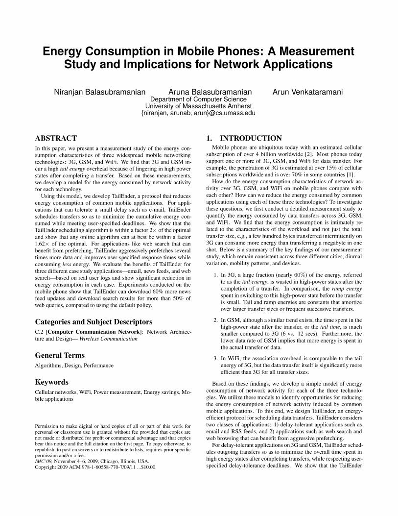
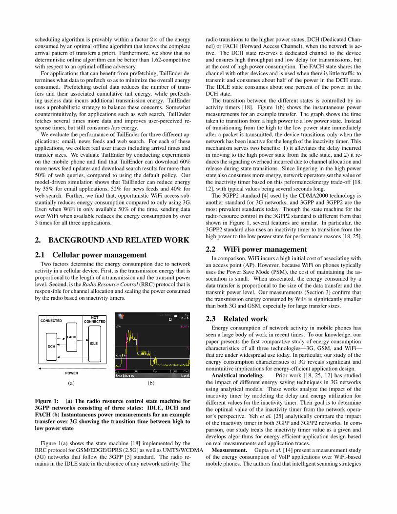
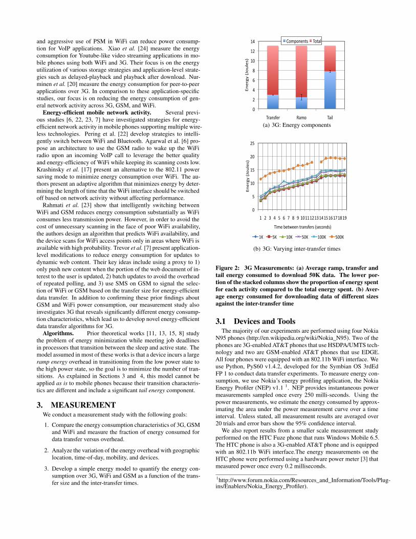
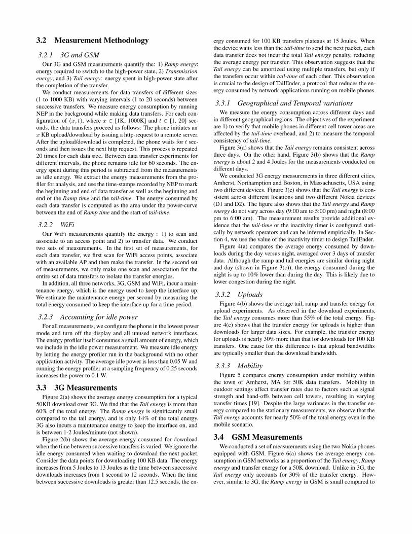

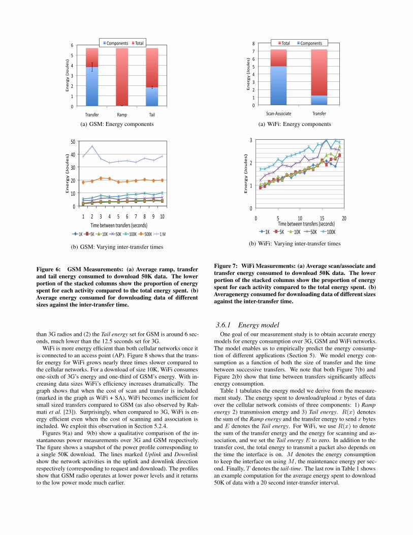


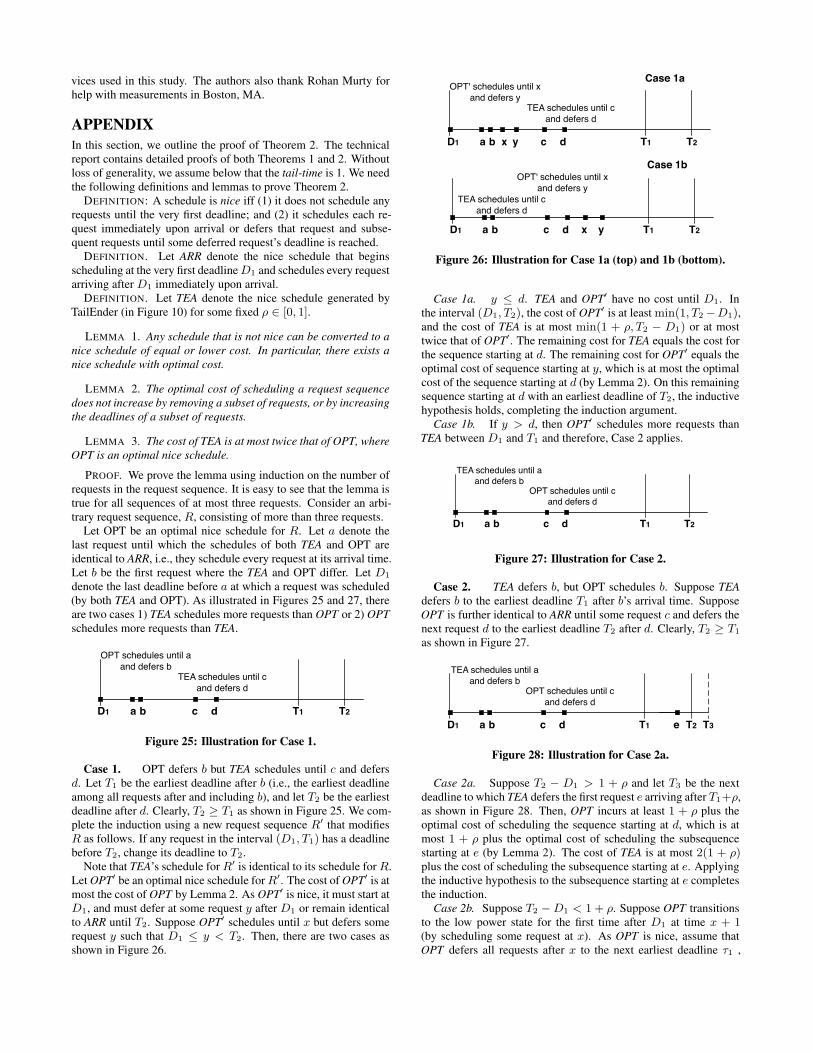
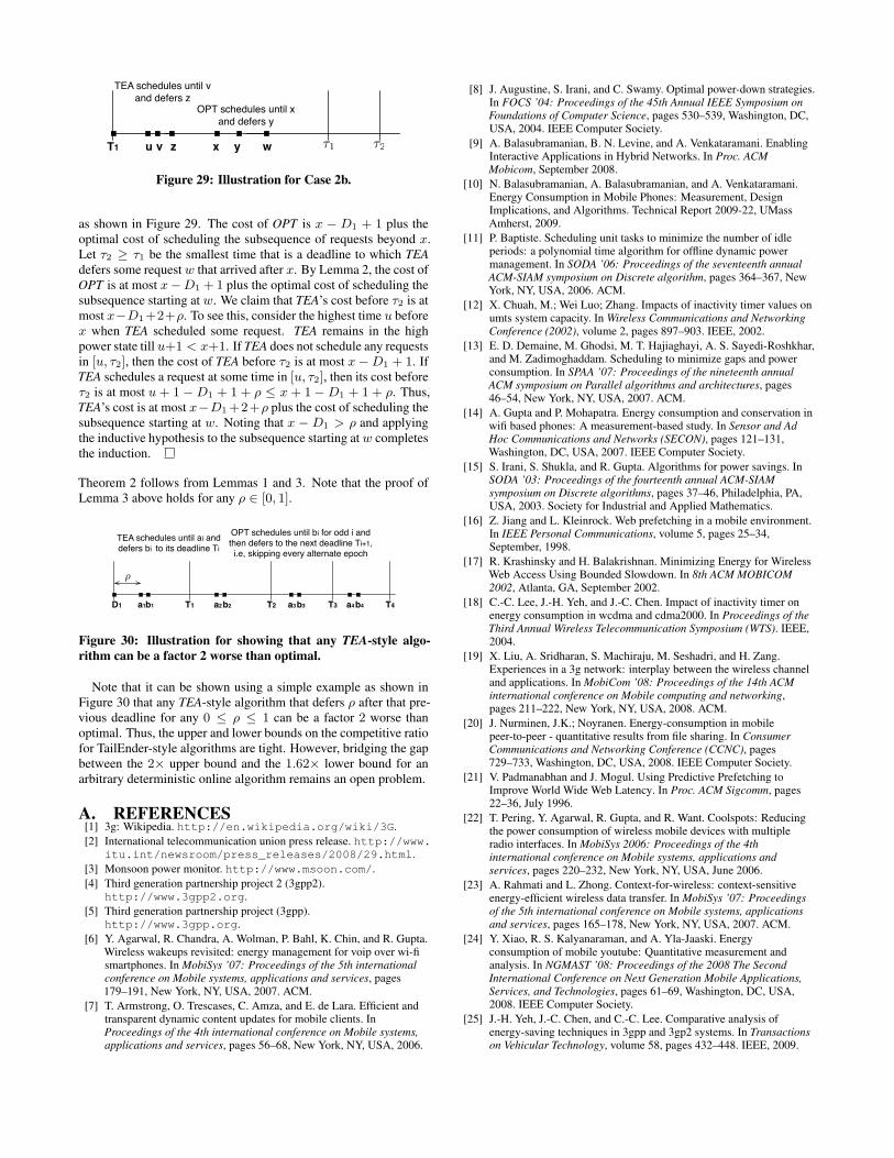
![Energy Consumption in Mobile Phones: A Measurement Study ... · Mobile phones are ubiquitous today with an estimated cellular subscription of over 4 billion worldwide [2]. Most phones](https://static.documents.pub/doc/80x56/5f7062b01d0b047cf77e0e1e/energy-consumption-in-mobile-phones-a-measurement-study-mobile-phones-are-ubiquitous.jpg)


