161

Energy Consumption of Error Control Coding Circuits
by
Christopher Graham Blake
A thesis submitted in conformity with the requirements
for the degree of Doctor of Philosophy
Graduate Department of Electrical and Computer Engineering
University of Toronto
c© Copyright 2017 by Christopher Graham Blake

Abstract
Energy Consumption of Error Control Coding Circuits
Christopher Graham Blake
Doctor of Philosophy
Graduate Department of Electrical and Computer Engineering
University of Toronto
2017
The energy complexity of error control coding circuits is analyzed within the Thompson
VLSI model. It is shown that fully-parallel encoding and decoding schemes with asymp-
totic block error probability that scales as O (f (N)) where N is block length (called
f(N)-coding schemes) have energy that scales as Ω(√
ln f (N)N). As well, it is shown
that the number of clock cycles (denoted T (N)) required for any encoding or decoding
scheme that reaches this bound must scale as T (n) ≥√
ln f (N). Similar scaling results
are extended to serialized computation.
Sequences of randomly generated bipartite congurations are analyzed; under mild
conditions almost surely such congurations have minimum bisection width proportional
to the number of vertices. This implies an almost sure Ω(N2/d2max) scaling rule for
the energy of directly-implemented LDPC decoder circuits for codes with maximum
node degree dmax. It also implies an Ω(N3/2/dmax) lower bound for serialized LDPC
decoders. It is also shown that all (as opposed to almost all) capacity-approaching,
directly-implemented non-split-node LDPC decoding circuits, have energy, per iteration,
that scales as Ω(χ2 ln3 χ
), where χ = (1 − R/C)−1 is the reciprocal gap to capacity, R
is code rate and C is channel capacity.
It is shown that all polar encoding schemes of rate R > 12of block length N imple-
mented according to the Thompson VLSI model must take energy E ≥ Ω(N3/2
). This
lower bound is achievable up to polylogarithmic factors using a mesh network topology
dened by Thompson and the encoding algorithm dened by Arkan. A general class of
circuits that compute successive cancellation decoding adapted from Arkan's buttery
ii

network algorithm is dened. It is shown that such decoders implemented on a rectangle
grid for codes of rate R > 2/3 must take energy E ≥ Ω(N3/2), and this can also be reached
up to polylogarithmic factors using a mesh network. Capacity approaching sequences of
energy optimal polar encoders and decoders, as a function of reciprocal gap to capacity
χ = (1−R/C)−1, have energy that scales as Ω (χ5.3685) ≤ E ≤ O(χ7.071 log4 (χ)
).
It is shown that all suciently large communication graphs of algorithms of bounded
degree can be implemented on a mesh network with routing conicts of size at most
log(N). This implies, conditioned on an assumption, that for all f(N) < e−O(N), and
f(N) encoding and decoding scheme can be constructed within a polylogarithmic factor
of the universal lower bounds for time and energy using a parallelized technique. Even
if the assumption is not true, the energy lower bounds can be reached up to a factor of
N ε polylog(N) using parallelized polar decoders, for any ε > 0.
The Grover information-friction energy model is generalized to three dimensions and
the optimal energy of encoding or decoding schemes with probability of block error Pe is
shown to be at least Ω(N (lnPe (N))
13
).
iii

Dedicated to my parents, Rob and Anuva.
iv

When I heard the learn'd astronomer,
When the proofs, the gures,
were ranged in columns before me,
When I was shown the charts and diagrams,
to add, divide, and measure them,
When I sitting heard the astronomer
where he lectured with
much applause in the lecture-room,
How soon unaccountable I became tired and sick,
Till rising and gliding out I wander'd o by myself,
In the mystical moist night-air, and from time to time,
Look'd up in perfect silence at the stars.
Walt Whitman
Acknowledgments
As I nish up my PhD I think back to my education; not just my graduate educa-
tion or my undergraduate education, but also the schooling I have done throughout my
life. As I think back on all of my teachers I remember a group of dedicated professionals
committed to the nurturing of knowledge and understanding. So the rst group of people
I would like to thank are all my teachers from pre-school, elementary school, high school,
undergrad, masters and nally PhD. I am also grateful to my Chinese teacher Hong
Laoshi and my piano teacher Mrs. Craig. From high school I am particularly grateful to
Ms. Werezak, my chemistry and geometry teacher, and Mr. Campbell, the person who
taught me calculus.
I want to also acknowledge and thank my fellow Kschischang-group colleagues. In
particular, I've been lucky to have the same group of labmates for a large portion of my
PhD, all of whom have been amazingly supportive and kind. I want to acknowledge, in
particular, Chen, Lei, Chunpo, Siddarth, and Siyu, who have been with me for most of my
PhD. I also want to acknowledge Christian Senger, a post-doc who has graciously given
me lots of advice and even helped me with the proofreading of some of my papers. As I
end my PhD all the people who were here when I started are now gone, and a new group
of students have arrived. I appreciate Frank's new students, Amir, Bo, Masoud, Reza,
and Susanna, and I am grateful to them for making our oce a warm and welcoming
place in the last few months of my PhD. I am also grateful to François Leduc-Primeau
for our discussions during his visits to U of T.
Throughout the PhD I have shared a lab with Professor Brendan Frey's students who
have all provided an enriching environment. In particular I'd like to thank Jeroen Chua,
my friend and machine learning guy who put particular eort into welcoming me into
v

the oce. I only wish that he was able to be my labmate for more than one year, but
I'm pretty sure that he'll eventually make an articially intelligent Jeroen robot that
we can just download and have an awesome labmate whenever we want.
My thesis involves a weird combination of ideas from computer science, physics, com-
puter engineering, and information theory. But I never formally studied computer science,
even though it is something that has always interested me. Fortunately, the theoretical
computer science community has proven to be an extraordinarily open community to
interact with. The Theoretical Computer Science Stack Exchange, for example, has a
clearly dedicated community. I've posted a number of questions to this community and
almost instantly received high quality answers! There are also a number of computer
science blogs of the highest quality. Of particular note is the blog of Scott Aaronson,
called Shtetl-Optimized, which to me is one of the best science resources ever created.
I am grateful to Pulkit Grover at Carnegie Mellon for welcoming me into his research
group for a month long visit to begin a research collaboration that I hope lasts for many
years. I also am thankful Pulkit Grover's student Haewon Jeong for pointing out some
of the weaknesses in an earlier version of the polar coding paper that formed the polar
coding chapter of this thesis, and for our continued collaboration. I also want to thank
JP, Maddie, Shervin, Rosario, Sarah and Elliot for making my stay in Pittsburgh such a
great time and for being such amazing people.
I am grateful to Professor David Asano for hosting me for a short visit to Shinshu
University in Nagano. I appreciate Professor Ian Blake (no relation) for hosting a talk
at UBC, and to Professor Sidharth Jaggi for hosting a talk at the Chinese University of
Hong Kong. Visiting professors at other Universities has been a highlight of my PhD
education and I appreciate the eort all these professors have put into making my visits
enjoyable and fullling.
There have been many professors who have helped and guided me along the way. In
undergrad, I am particular grateful to Tarek Abdelrahman for taking me on as a research
volunteer in the summer after my rst year. I am also grateful to Aleksandar Prodic for
taking me on as an undergraduate researcher after my second year. He also provided me
with a reference for my MIT application which must have been pretty good because I
got accepted! I am also grateful to Professor Jonathan Rose for calling me when I was
in high school and talking to me about ECE at U of T, and for continual encouragement
throughout my undergrad all the way to PhD. I also am thankful to Susan Grant for
providing such detailed answers to my questions when I was deciding whether to go to
U of T or other schools I got accepted to for undergrad.
Between my third and fourth year I worked at a company called Altera. I appreciated
vi

the experience working at what is a very successful company. In particular, I appreciate
Blair Fort for providing me with excellent mentorship and supervision. I also appreciate
the advice and guidance given by Stephen Brown and Zvonko Vranesic during this time.
I also want to thank Deshanand Singh for being an amazing cubicle neighbour during
most of my time at Altera and also providing me with a reference for my masters.
During my time at MIT I worked with Jerey Shapiro in the eld of quantum infor-
mation theory. I thank Professor Shapiro for giving me such an amazing opportunity to
work at what is clearly one of the best universities in the world. His guidance formed a
basis for my research skills that I took with me when I went back to Toronto. Also at
MIT I attended many excellent lectures. In particular, I want to thank Professors Muriel
Médard, Greg Wornell, and Alan Edelman for their wonderful lectures that I had the
privilege to attend. In particular I have made much use of Alan Edelman's observation
about the dierence between how one reads a mathematical proof and an engineering
proof. I also want to acknowledge Alan Oppenheim for providing such dedicated guid-
ance and mentorship to both me and a large number of my MIT colleagues. Among my
MIT colleagues I am particularly grateful to Hung-Wen and Mansoo for being such great
language exchange partners.
I'd like to thank my thesis committee, including Glenn Gulak, Stark Draper, Wei Yu,
and Anant Sahai for their detailed reading of the thesis and challenging and interesting
discussions. I particularly appreciate Anant Sahai for coming all the way from Berkeley
for my defense and for his very positive review of my thesis.
The next person that I should acknowledge probably goes without saying. Of course,
this person is my advisor, Frank Kschischang. I rst saw him more than twelve years ago
when I was in high school at a recruiting event for high school students. He presented an
introduction to the eld of coding theory, and he did so by presenting a simple Hamming
code to a bunch of high school students and their parents. It was probably then that
I decided my eld of research that I have continued studying to this day. When I was
accepted to MIT Frank met with me numerous times advising me about going to MIT
and his advice was useful. When I decided in my second year of my masters that I wanted
to spend my PhD back at the University of Toronto, Frank welcomed me into his group.
The choice to go back to Toronto was a unique choice, but in the last ve years I am happy
to say I have no regrets. Frank's dedication to my professional development has gone far
beyond even my most optimistic of expectations. He has given me an extraordinary level
of freedom and trust in pursuing my research in my own way. In our discussions Frank
has consistently proven an amazing ability to almost always come up with surprising and
helpful insights. He is a scientist of the highest calibre, and it has been an honour to be
vii

his student.
I also want to thank my parents and my grandparents for their love and support
throughout my life. I'd also like to thank my brothers, Aaron and Raymond, my nephew
Jagger, my aunts, uncles, and cousins. In particular for this thesis I want to acknowledge
Aunt Korobi and Uncle Babu for all the academic encouragement throughout my life.
Also, I want to acknowledge my cousins Santanu and Sonali for being examples of what
life can be like if you spend a really, really long time doing school.
I want to say particular thanks to my friends with whom I have shared so many
amazing adventures during this PhD. Without all of you my thesis would have been
done more quickly, but it would have been much worse. There are many friends who t
this category, but in particular, thank you to Keith, David, Tommy, David (yep, that's a
second David, I know a lot of Davids), Sandy, Tomoki, Yenson, Bill, Sina, Simon, Amer,
Matt, Jenn, Yijun, Palermo, Pickles, Fengyuan, Shilin, Galen, Mark, Will Li, Peng, Kyu,
Dmitry, and Daniel for all the amazing adventures.
As I write this last paragraph of my thesis on a cold December afternoon in Toronto,
thinking about what I'm going to do now that I have a PhD, I don't know what lies
ahead. Usually in these situations I just do the next thing you do to get a PhD, but now
my formal education has come to an end. For what I do next I can think of a universe of
possibilities, all of them interesting, but none of them certain. Thus, I choose to end this
section with a quote that seems relevant, which was presented by Anant Sahai in a talk
he gave at the University of Toronto the day after my nal examination. It is a line from
a paper written by Claude Shannon, that, coincidentally perhaps, has some relevance to
my situation right now: ...we may have knowledge of the past but cannot control it; we
may control the future but have no knowledge of it. I don't know what my future will
bring, but I thank all my educators for giving me the tools to control it.
viii

Contents
1 Introduction 1
1.1 Introduction . . . . . . . . . . . . . . . . . . . . . . . . . . . . . . . . . . 1
2 Thompson Model 4
2.1 The Thompson Model . . . . . . . . . . . . . . . . . . . . . . . . . . . . 4
2.2 Discussion of Model . . . . . . . . . . . . . . . . . . . . . . . . . . . . . . 8
2.3 Related Literature . . . . . . . . . . . . . . . . . . . . . . . . . . . . . . 13
2.4 Other Energy Models of Computation . . . . . . . . . . . . . . . . . . . . 15
3 General Lower Bounds 17
3.1 Prior Related Work . . . . . . . . . . . . . . . . . . . . . . . . . . . . . 18
3.2 Denitions and Lemmas . . . . . . . . . . . . . . . . . . . . . . . . . . . 19
3.3 Nested Bisections . . . . . . . . . . . . . . . . . . . . . . . . . . . . . . . 21
3.4 Main Lower Bound Results . . . . . . . . . . . . . . . . . . . . . . . . . . 25
3.5 Serial Decoding Scheme Scaling Rules . . . . . . . . . . . . . . . . . . . . 30
3.6 Encoder Lower Bounds . . . . . . . . . . . . . . . . . . . . . . . . . . . . 34
3.7 Asymptotic Probability of Error Approaching a Constant . . . . . . . . . 35
4 LDPC Codes 36
4.1 Prior Work . . . . . . . . . . . . . . . . . . . . . . . . . . . . . . . . . . 37
4.1.1 Related Work on Circuit Complexity and LDPC codes . . . . . . 37
4.1.2 Related Work on Graph Theory . . . . . . . . . . . . . . . . . . . 38
4.2 Directly-Implemented LDPC Decoders . . . . . . . . . . . . . . . . . . . 38
4.3 Serialized LDPC Decoders . . . . . . . . . . . . . . . . . . . . . . . . . . 41
4.4 Almost Sure Scaling Rule . . . . . . . . . . . . . . . . . . . . . . . . . . 42
4.5 Almost Sure Bounds on Suciently High Rate LDPC Decoder Circuits . 50
4.5.1 Energy Complexity of Directly-Implemented LDPC Decoders . . . 51
ix

4.5.2 Serialized Decoders . . . . . . . . . . . . . . . . . . . . . . . . . . 52
4.5.3 Applicability and Limitations of Result . . . . . . . . . . . . . . . 56
4.6 Bounds for All Directly-Implemented Non-Split-Node LDPC Decoder Cir-
cuits . . . . . . . . . . . . . . . . . . . . . . . . . . . . . . . . . . . . . . 57
4.7 Tight Upper Bound for Directly-Implemented LDPC Decoders . . . . . . 59
5 Polar Codes 62
5.1 Prior Related Work . . . . . . . . . . . . . . . . . . . . . . . . . . . . . . 64
5.2 Polar Encoders Lower Bound . . . . . . . . . . . . . . . . . . . . . . . . 64
5.2.1 Rectangle Pairs . . . . . . . . . . . . . . . . . . . . . . . . . . . . 64
5.2.2 Universal Polar Coding Generator Matrix Properties . . . . . . . 66
5.2.3 Encoder Circuit Lower Bounds . . . . . . . . . . . . . . . . . . . 68
5.3 Arkan Successive Cancellation Polar Decoding Scheme . . . . . . . . . . 70
5.3.1 Polar Decoding Lower Bound Preliminaries . . . . . . . . . . . . . 70
5.3.2 Decoder VLSI Lower Bounds . . . . . . . . . . . . . . . . . . . . 76
5.4 Upper Bounds . . . . . . . . . . . . . . . . . . . . . . . . . . . . . . . . . 77
5.4.1 Mesh Network . . . . . . . . . . . . . . . . . . . . . . . . . . . . . 77
5.4.2 Encoding . . . . . . . . . . . . . . . . . . . . . . . . . . . . . . . 79
5.4.3 Analysis of Mesh Network Encoding Algorithm Complexity . . . . 80
5.4.4 Decoding Mesh Network . . . . . . . . . . . . . . . . . . . . . . . 81
5.5 Generalized Polar Coding on a Mesh Network . . . . . . . . . . . . . . . 81
5.6 Energy Scaling as Function of gap to Capacity . . . . . . . . . . . . . . . 82
6 Mesh Networks 84
6.1 Mesh Network . . . . . . . . . . . . . . . . . . . . . . . . . . . . . . . . . 85
6.2 Communication Protocols with Low κmax Exist For Most Graphs . . . . . 87
6.2.1 LDPC Codes on a Mesh Network . . . . . . . . . . . . . . . . . . 96
6.3 Using Parallelization to Construct Close to Energy Optimal f(N)-coding
Schemes . . . . . . . . . . . . . . . . . . . . . . . . . . . . . . . . . . . . 97
6.3.1 Analyzing Area and Number of Clock Cycles . . . . . . . . . . . . 98
7 Information Friction in
Three-Dimensional Circuits 100
8 Is the Information Friction Model a Law of Nature? 107
8.0.2 The Spaceship Channel . . . . . . . . . . . . . . . . . . . . . . . . 108
8.0.3 The Vacuum Tube Channel (AKA the Hyper-loop Channel) . . . 108
x
8.0.4 Electromagnetic Radiation . . . . . . . . . . . . . . . . . . . . . . 109
8.0.5 Quantum Entanglement . . . . . . . . . . . . . . . . . . . . . . . 109
8.0.6 Adiabatic Computing . . . . . . . . . . . . . . . . . . . . . . . . . 109
8.0.7 Superconducting Channel . . . . . . . . . . . . . . . . . . . . . . 110
8.0.8 The Wormhole Circuit . . . . . . . . . . . . . . . . . . . . . . . . 110
9 Conclusion 111
A Appendices 115
A.1 Coding Schemes with Error Probability Less than 1/2 . . . . . . . . . . . 115
A.1.1 Bound on Block Error Probability . . . . . . . . . . . . . . . . . . 117
A.1.2 Fully Parallel Lower Bound . . . . . . . . . . . . . . . . . . . . . 119
A.1.3 Serial Computation . . . . . . . . . . . . . . . . . . . . . . . . . . 121
A.1.4 A General Case: Allowing the Number of Output Pins to Vary
with Increasing Block Length . . . . . . . . . . . . . . . . . . . . 124
A.2 Denition of δ(L,R) in Terms of Node Degree Distributions . . . . . . . 129
A.3 Proof of Lemma 9 . . . . . . . . . . . . . . . . . . . . . . . . . . . . . . . 130
A.4 Proof of Lemma 9 Continued . . . . . . . . . . . . . . . . . . . . . . . . 131
A.5 Proof of Theorem 6 . . . . . . . . . . . . . . . . . . . . . . . . . . . . . . 132
A.6 Proof of Lemma 13 . . . . . . . . . . . . . . . . . . . . . . . . . . . . . . 135
A.7 Proof Of Lemma 21 . . . . . . . . . . . . . . . . . . . . . . . . . . . . . . 140
A.8 Mesh Network Polar Encoding Procedure . . . . . . . . . . . . . . . . . . 140
Bibliography 142
xi

There is a fact, or if you
wish, a law, governing all
natural phenomena that are
known to date. There is
no known exception to this
lawit is exact so far as we
know. The law is called the
conservation of energy. It
states that there is a certain
quantity, which we call en-
ergy, that does not change in
the manifold changes which
nature undergoes.
Richard Feynman 1Introduction
1.1 Introduction
The central topic of this thesis is: what are the fundamental energy limits of communi-
cation of information in our universe? Traditionally, Shannon's channel coding theorem
has provided a satisfying answer: Channels through which we would like to communi-
cate information are associated with a probability distribution. From this distribution
a quantity called capacity can be computed. For a given channel, rates below capacity
can be achieved using a suciently clever error control coding scheme. Rates above this
capacity cannot be achieved reliably. Generally speaking, transmitting a message with
more energy changes the underlying channel statistics, and this increases the capacity.
This would be a satisfactory answer to the central topic of this thesis, except Shan-
non's channel coding theorem assumes an encoder and decoder, which in practice are
usually specialized circuits that compute error control coding functions. These circuits
consume energy. Thus, in this thesis we study the energy complexity of circuits that com-
pute error control encoding and decoding functions. In doing so, we will gain insights
into the fundamental energy limits of computation in general.
Thus, in Chapter 2 we present an adaptation of Thompson's VLSI model [1], which
we use to model the energy consumption of VLSI circuits. The model also allows us to
1

Chapter 1. Introduction 2
consider energy-time tradeos. We call this model the Thompson model.
Our rst main technical results are presented in Chapter 3. In this chapter, we
use a simplication of the approach of Grover et al. [2] to derive scaling rule lower
bounds for encoding and decoding schemes for binary erasure channels classied according
to how their associated block error probability scales with increasing block length N .
In particular, we dene an f(N)-coding scheme as a sequence of codes, encoders, and
decoders for a particular channel that have block error probability that scales as O(f(N)).
In particular, we show that all fully-parallel f(N)-coding schemes have encoding and
decoding energy lower bounded by Ω(N√
log(f(N))). Similar bounds are derived for
serial implementations. Having derived these universal complexity lower bounds, in the
chapters that follow we analyze existing decoding algorithms to see how their complexity
compares. The discussion eventually leads to Chapter 6 which shows how to construct
fully-parallel f(N)-coding schemes that almost reach the universal lower bounds.
The rst class of codes we analyze in Chapter 4 are LDPC codes. Such codes utilize
the sparsity of a linear code's parity check matrix for ecient decoding. In their anal-
ysis, graphs are often generated according to a uniform conguration distribution. We
show, subject to some mild conditions, that the minimum bisection width of a randomly
generated bipartite conguration asymptotically almost surely has minimum bisection
width proportional to the number of vertices. For degree distributions with maximum
node degree dmax, this implies an Ω(N2/d2max) lower bound on the energy of directly-
implemented LDPC decoders (see Denition 24) and a Ω(N3/2/dmax) lower bound on the
energy of serialized decoders (see Denition 33). For dmax that does not increase with N ,
we show how to construct a directly-implemented circuit that reaches this lower bound in
this chapter. Later, in Chapter 6 we show that the serialized lower bound can be reached
using a mesh network up to a polylogarithmic factor.
The second class of codes that we analyze are polar codes [3]. In this section we
analyze polar codes of suciently high rate. We exploit the recursive structure of the
polar coding generator matrix to prove a property about the ranks of sets of submatrices
of the generator matrix called rectangle pairs. This is used to derive a Ω(N1.5) energy
lower bound on polar encoders. The encoding lower bound applies to any circuit that
computes a polar encoding function; for polar decoding, on the other hand, it is more
dicult to dene a valid decoding method. However, Arkan [3] suggests a successive
cancellation decoding technique based on the buttery network graph. Thus, the other
main result in this section proves an Ω(N1.5) lower bound on the energy complexity of
such decoders. We then show how the mesh network topology approach of [1] can be
adapted for polar encoding to reach this lower bound up to a polylogarithmic factor. For

Chapter 1. Introduction 3
polar decoding the energy lower bounds can also be reached with a mesh network up to
a polylogarithmic factor.
Having shown how to use the mesh network topology to perform polar encoding and
decoding, we further analyze the mesh network and show that, in fact, all algorithms
with communication graphs of bounded vertex degree can be implemented with a mesh
network. The main idea is to use the probabilistic method to show that there exists
a placement of nodes on the mesh network that avoids large conicts. Conditioned on
an assumption about the iterative performance of LDPC codes, this implies there exists
e−Θ(N)-coding schemes that have energy that scales close to O(N1.5). We then show
how parallelization can be used to construct an f(N)-coding scheme that comes close
to the universal time and energy lower bounds. Even if the assumption is not true, we
also discuss how universal energy lower bounds (but not the time lower bounds) can be
almost reached using generalized polar codes of [4].
Up to this point our results involve planar circuits. In Chapter 7 we expand our
lower bound analysis to three dimensions. We adapt the two-dimensional information-
friction model of Grover [5] to three dimensions and prove lower bounds for encoders
and decoders in terms of block error probability. In particular, we show that encoders
and decoders have energy E ≥ Ω(N(− log(Pe)1/3)) for codes of block length N and block
error probability Pe.
In Chapter 8 we examine the information friction model and build upon the discus-
sions of Grover [5] and analyze a number of communication schemes that may seem to
violate the assumptions of the model. However, we show that upon further analysis such
schemes have either have linear or worse energy per bit as a function of distance, or, for
one reason or another, they are utterly impractical.
Finally, in Chapter 9 we summarize the main scaling rule results and discuss some
areas of future work.
Notation: We use standard Bachmann-Landau [6, 7] notation in this thesis. The
statement f(x) = O(g(x)) means that for suciently large x, f(x) ≤ cg(x) for some
positive constant c. The statement f(x) = Ω(g(x)) means that for suciently large x,
f(x) ≥ cg(x) again for some constant c. The statement f(x) = Θ(g(x)) means that
there are two positive constants b and c such that b ≤ c and for suciently large x,
bg(x) ≤ f(x) ≤ cg(x).

Now it would be very remarkable if any sys-
tem existing in the real world could be exactly
represented by any simple model. However,
cunningly chosen parsimonious models often
do provide remarkably useful approximations.
For example, the law PV = RT relating pres-
sure P, volume V and temperature T of an
"ideal" gas via a constant R is not exactly
true for any real gas, but it frequently provides
a useful approximation and furthermore its
structure is informative since it springs from a
physical view of the behavior of gas molecules.
For such a model there is no need to ask the
question Is the model true?. If truth is to
be the whole truth the answer must be No.
The only question of interest is "Is the model
illuminating and useful?.
George Box
2Thompson Model
2.1 The Thompson Model
The central mathematical object of this thesis is the circuit, which is adapted from the
work of Thompson [8] which we call the Thompson model. Note however that our model
is slightly dierent from the models discussed in [8], but for the purposes of our lower
bound scaling rules, none of these dierences matter. In this section we describe the
circuit mathematically, with little reference to the real-life circuits from which the model
is inspired. Then in Section 2.2 we discuss how the model relates to actual circuit design,
and address a number of possible objections to the model. The main idea of the model
is that a circuit is a set of nodes and wires laid out on a grid of squares, and energy
consumption comes from switching the values stored in these grid squares.
A circuit is a mathematical object C, finput, foutput consisting of a circuit grid C, aninput protocol finput, and an output protocol foutput which we dene below. After the
denition of a circuit, we will give two examples of a circuit, and then show how such
circuits compute functions.
• A circuit grid is a collection of nodes and wires laid out on a planar grid of squares.
Each grid square can be empty, can contain a computational node (sometimes
referred to more simply as a node), a wire, or a wire crossing. A circuit also
4

Chapter 2. Thompson Model 5
Figure 2.1: Diagram of a possible VLSI circuit. Grid squares that are fully lled inrepresent computational nodes and the lines between them represent wires. Note that inthe upper-left quadrant of the grid there is a wire crossing.
Figure 2.2: The six types of wire-nodes drawn on a grid square. In the obvious way thesenodes can be placed together to connect to form paths between computational nodes ina circuit.
has some special nodes called input nodes and also output nodes. We let there
be I input nodes in the circuit and J output nodes. The purpose of a circuit is
to compute a function f : (0, 1)Ninput → (0, 1)Noutput . Such a circuit is said to have
Ninput inputs and Noutput outputs. Note that the number of function inputs/outputs
may not be the same as the number of input/output nodes, since input/output can
be serialized. The computation is divided into T clock cycles, and the Ninput inputs
are to be injected into the I input nodes during some clock cycle, and the Noutput
outputs are to appear in the J output nodes during some clock cycle.
• Each grid that contains a wire may be either a horizontal, vertical, or bending wire.
Each wire grid has associated with it its connecting sides. In the diagrams of these
grid squares, these are simply the the sides of the square that the wire touches. See
Figure 2.2 for a diagram of the six types of wire nodes.
• Two grid squares containing wires are connected if the they have adjacent connecting
sides. Now, obviously, we see that adjacent wire nodes can form a path between
computational nodes in the natural way.

Chapter 2. Thompson Model 6
• Conceptually, computational nodes are the computing parts of the circuit. There
are two types of computational nodes: logic nodes and register nodes.
• Each node has at most 4 wires connected to it, which are used to feed in bits into
the node and feed out the bits computed by the node. Each of the four sides of a
computational node is associated with either input or output. A wire may connect
to an input or output side of a computational node. A path starting at such a wire
may lead to another computational node. For a circuit to be valid wire paths may
only connect output sides to input sides.
• A register node has one input side and up to three output sides. Conceptually, the
purpose of a register node is to store information until the next clock cycle.
• A logic logic node is associated with a function. A logic node with κinput input sides
and κoutput output sides can compute any function g : 0, 1κinput → 0, 1κoutput .So, for example, a possible logic node may have three input sides, associated with
input x1, x2, x3 and one output side associated with output y1. Then such a node
may compute the function which is the logical AND the three inputs. That is
g(x1, x2, x3) = x1 ∧ x2 ∧ x3.
• An input node is a special type of register node in the circuit which has no input
side. Conceptually, the value in this register depends on the current input to the
node at the most recent clock cycle. In the state update rule for the circuit (which
we dene below), after each clock cycle, the value on wires adjacent to the input
node shall be updated to the value of the input.
• An output node is another special type of register node in a circuit. The output
node is required to hold in its output bit some circuit output during pre-determined
clock cycles.
• Each wire and computational node is associated with a state. The wires and the
register nodes may be in state 0 or state 1. The state of a wire crossing is associated
with two bits: one for each wire in the wire crossing. We let the vector of all states
of the nodes be S, and the set of all possible states for a particular circuit be S.We let the set of possible input node states beMinput.
• There is a natural update rule for the circuit. The update rule is a function fupdate :
S ×Minput → S that maps the current state of the circuit and circuit inputs to the
state of the circuit at the next clock cycle. The update rule function is the function

Chapter 2. Thompson Model 7
induced by the natural evaluation of the circuit: each computational node computes
their functions and then alters the state of the wires at their output. Then, the
state of all wires that are adjacent are set equal. When wires are adjacent to the
inputs of logic nodes, the wires at the output of the logic nodes are changed to
the evaluation of their function. The wire values are updated until they reach the
input of a register node.
Note that for a circuit to be valid, there should be no wires unconnected to
computational nodes. From this point on we will be discussing only valid
circuits; that is, those whose update rule is well dened.
• An input-output protocol is an ordered pair of functions (finput, foutput) where finput :
[Ninput] → [I] × N is a function called the input protocol, that takes in as input a
number representing the ith input bits, and the output is a an ordered pair (a, b)
where a is interpreted as the input node into which that input bit is to be inserted,
and b is the clock cycle of the computation that the input bit is to be inserted.
Similarly, foutput : [Noutput]→ [O]× N is a function called the output protocol. The
output protocol is dened similarly, mapping an output bit index to an output node
and clock cycle. The input/output protocols can be interpreted as a table.
In Example 1 we see an example of a fully parallel circuit with a table representing
its input/output protocol. We see another example of a circuit which computes
a similar function, but has a dierent circuit layout and a serialized input-output
protocol in Example 2.
• Given a particular input, a circuit grid and an input-output protocol, one can
determine the output of the circuit given this input. This can be done for all
possible inputs to the function. Thus, associated with the circuit is the circuit
function that the circuit computes, which is the function mapping the set of all
possible input values to their output when the input-output protocol is used.
• The area of a circuit is the number of grid squares occupied by either a wire or a
node, denoted A.
• The number of clock cycles is the clock cycle number during which the last output
bit is to appear, which we denote T .
• The energy of a computation given a particular inputMinput, denoted Ecomp(Minput)
is proportional to the number of node state changes that occurred during the com-
putation. Note that the constant of proportionality relating these quantities is

Chapter 2. Thompson Model 8
technology dependent, but since we are concerned with scaling rules in terms of
increasing circuit size, we simply set this constant of proportionality to unity.
• The worst case energy of a computation is E = maxx∈0,1Ni Ecomp(x). Note that
the results in this thesis are about worst case energy bounds.
• The switching activity factor is denes as q = EAT
, and is the average fraction of
nodes or wires in the circuit that switch during the computation. Note that for
many of the proofs involving scaling rules as a function of block length N in this
thesis, a switching activity that is bounded below as a function of block length N
is assumed. With such an assumption the energy of a computation can be bounded
by E ≥ qAT .
2.2 Discussion of Model
In this section we discuss the justication for this model, as well as address a number of
objections to and limitations of the model.
Energy Proportional to Area-Time Product
The main idea of the model is that in modern VLSI circuits, wires are charged or dis-
charged each clock cycle whenever their state changes. This process consumes energy,
because the wires have some capacitance. From electromagnetics, it is known that the
energy to charge a capacitor with capacitance Cc at voltage Vc is equal to E = 12CcV
2c .
Since wires are laid out essentially at, they have a capacitance roughly proportional to
their area. Thus, in our model, the energy to charge and discharge a wire is proportional
to the number of grid squares it occupies. With switching activity factor q the number
of switches a circuit undergoes in a computation is proportional to qAT .
Time and Number of Clock Cycles
Note that our quantity T refers to number of clock cycles, which reects one of the main
time costs in a circuit computation. In real circuits, the time cost of a computation
involves two parameters: the number of clock cycles required, and the time it takes to
do each clock cycle. In our model, we do not consider the time per clock cycle. In real
circuits, this quantity often varies with wire lengths. Chazelle et al. [9] introduce a
renement of the Thompson model that considers wire length costs. We do not consider
this in this thesis.

Chapter 2. Thompson Model 9
Example 1 Parallel Circuit Example
j1 j2 j3 j4
⊕ ⊕
o1
⊕
An example of a circuit grid. The four input nodes of this circuit are labelled j1, j2, j3, j4,two logic nodes are labelled with the ⊕ symbol, and the single output node is labelledwith an o1. In this particular circuit, information ows from top to bottom in the wires.The following table represents the input protocol of the circuit:
Input Input node Clock cycle
1 1 12 2 13 3 14 4 1
As well, the output protocol for this circuit is:Output Output node Clock Cycle
1 1 1The ⊕ node computes the XOR function. Note that this circuit is fully parallel.To see how this circuit behaves, we simply follow the update rule. At the rst clock cyclethe 4 input bits are loaded into the 4 input nodes. These values ow into the two ⊕ logicnodes, and then after the second clock cycle these values are stored in the single outputregister. It is thus easy to see that the function that this circuit computes is the mod 2sum of the 8 input bits. The area A of this circuit is 21, as this is how many grid squaresare occupied.

Chapter 2. Thompson Model 10
Example 2 Serial Circuit Example
⊕ ⊕
j1 j2 j3 j4
⊕
⊕
>
R
o1
An example of a serialized circuit. The four input nodes of this circuit are labelledj1, j2, j3, j4, two logic nodes are labelled with the ⊕ symbol, and the single output nodeis labelled with an o1. The nodes labelled ⊕ compute the XOR of their inputs. The nodelabelled > computes the t-joint function, and takes in as input the bit from the rightand outputs this bit at its left and the bottom. The node labelled with R is a registernode. This circuit computes a function of 8 inputs, but has only 4 input nodes.To see how this circuit behaves, we simply follow the update rule. At the rst clock cyclethe 4 input bits are loaded into the 4 input nodes. These values ow into the two ⊕ logicnodes, and then after the second clock cycle these values are stored in the single outputregister. It is thus easy to see that the function that this circuit computes is the mod 2sum of the 4 input bits.The area A of this circuit is 34.This circuit has the following input protocol:
Input Input node Clock cycle
1 1 12 2 13 3 14 4 15 1 26 2 27 3 28 4 2
The output protocol for this circuit is:Output Output node Clock Cycle
1 1 2

Chapter 2. Thompson Model 11
Leakage Current
In modern digital circuits, leakage current is an unavoidable eect where energy is con-
sumed when electrons or holes tunnel through insulated regions of the circuit. In circuit
design, sometimes this leakage current is factored into energy models of computation
(see [10] and [11]). However, we neglect leakage current in our model. To justify this
assumption, we can assume the frequency of computation is high enough so that the
energy used in charging and discharging the wires dominates.
Logic Gates of Dierent Size or Energy Consumption
Note that the restriction that each node has in total at most four inputs and outputs
is somewhat arbitrary; it is also arbitrary that each node is permitted to compute any
function of its inputs all at the same area and energy cost. In real VLSI implementations
it may be that an arrangement of transistors can compute some functions more eciently
than others. However, our model does not consider what gains could be made if certain
functions are cheaper in an energy sense to compute. However, models that vary the
size and energy consumption of dierent logic gates can only change the circuit area
by a constant amount and so our model simply assumes any logic gate with up to four
input/output wires can be implemented in unit area.
Multiple Layer VLSI Circuits
Modern VLSI circuits dier from the Thompson model in that the number of VLSI layers
is not one (or two if one counts a wire crossing as another layer). Modern VLSI circuits
allow multiple layers. Fortunately, it is known that if L layers are allowed, then this can
decrease the total area by at most a factor of L2 (see, for example, [1] or [12]). For the
purposes of our lower bounds, if the number of layers remains constant as input size N
increases, we can modify our energy lower bound results by dividing the lower bounds by
L2. If, however, the number of layers can grow with N our results may no longer hold.
Note also that this only holds for the purpose of lower bound. It may not be possible
to implement a circuit with an area that decreases by a factor of L2, and so the upper
bounds cannot be similarly modied for multiple layer circuits.
Multiple Switches in Each Clock Cycle
In our model, we assume that at each clock cycle a wire can switch at most one time.
However, in real circuits, the inputs into a logic node may change multiple times each
clock cycle because dierent inputs for each logic gate change at slightly dierent times
Chapter 2. Thompson Model 12
(owing to dierences in wire lengths and logic gate delays). This motivated Aggarwal et
al. to introduce the multi-switch energy consumption model of [13]. The authors argue
that if a gate is at depth h in a circuit, and the circuit has fan-in c, the output of this
logic gate can switch up to ch times each clock cycle. This could be a signicant factor in
the energy of a computation but we do not consider this here in either our lower bounds
or upper bounds. A similar model was introduced by Kissin [14].
Multiswitching is a possible signicant source of energy consumption. However, I
conjecture that in real circuits the energy consumption caused by multiswitching cannot
grow too large (that is, it cannot grow signicantly quickly as a function of N) because
resistive-capacitive eects of the wires will slow down the charging and discharging of the
wires if the output of a gate is switched too frequently.
Using Memory Elements in Circuit Computation
The Thompson model does not allow for the use of special memory nodes in computation
that can hold information and compute the special function of loading and unloading from
memory. Such a circuit can be created using the Thompson model, but it may be that
a strategic use of a lower energy memory element can decrease the total energy of a
computation. However, the use of a memory element to communicate information within
a circuit is still proportional to the distance that information is communicated (See for
example the analysis of [15] where the main energy consumption of dynamic random
access memories ows from charging and discharging capacitors as in the Thompson
model, or our discussion in Chapter 8 justifying the linear in distance energy assumption).
With only a linear-in-distance energy consumption assumption Grover in [5] proposed a
bit-meters model of energy computation and derives energy scaling rules similar to our
fully parallel results. We generalize the Grover bit-meters model to three dimensions in
Chapter 7.
Though the information friction analysis suggests that using memory will not change
the rst order scaling results of this thesis, the proportionality constants relating distance
communicated to energy may be signicantly dierent for memory usage compared to
energy consumed in wires and logic gates. Thus, in real circuit designs balancing wire
and memory energy consumption may be an area of signicant practical and theoretical
interest that is beyond the scope of this thesis.

Chapter 2. Thompson Model 13
2.3 Related Literature
In [8] it was proven that the area-time complexity of any circuit implemented according
to this VLSI model that computes a Discrete Fourier Transform must scale as Ω (N1.5).
However, there exist algorithms that compute in O (N logN) operations (for example,
see [16]); Thompson's results thus imply that, for at least some algorithms, energy con-
sumption is not merely proportional to the computational complexity of an algorithm.
Related to the Thompson model is the computational problem of laying out a graph
on a plane. This problem has been shown to be NP-Complete by Dolev et al. in [17].
The Thompson model, in addition to being studied for sorting and discrete Fourier
transform by Thompson in [1] has also been studied for dierent computational problems.
Vuilleman [18] shows how a number of computational problems, including cyclic shifts,
linear transforms, and cyclic convolution have analytical expressions for lower bounds on
their area-time complexity because the functions such circuits compute all have a similar
mathematical property.
Tyagi [19] denes a concept called information complexity of a function, which im-
plies lower bounds on a circuit's area-time complexity. The information complexity of
a function is the number of bits that have to be communicated between any two equal
sized partitions of the input bits. Tyagi's approach is very similar to our approach, and
in fact our lower bounds for polar encoding and decoding, as well as LDPC decoding can
be interpreted as nding lower bounds on this information complexity parameter for the
functions that they compute. However, this information complexity measure does not
extend to our general lower bounds of Chapter 3, mainly because our lower bounding
technique uses the nested bisection technique used by Grover [2], as opposed to a single
bisection.
Related to the concept of information complexity is the widely studied computer
science concept of communication complexity [20]. The communication complexity is
dened for functions to be computed by two parties, where one party has one half of the
input bits and the other party has the other half. The communication complexity then
is the minimum number of bits that must be communicated between the two parties so
that either one of the parties can compute the function. The information complexity
discussed in the previous paragraph can then be dened as the minimum communication
complexity over all possible bisections of the input bits.
The earliest work on computational complexity lower bounds for good decoding comes
from Savage in [21] and [22], which considered bounds on the memory requirements and
number of logical operations needed to compute decoding functions. However, wiring

Chapter 2. Thompson Model 14
area is a fundamental cost of good decoding and the authors do not consider this. More
recently, in [23], the authors use a model similar to our model, except the notion of area
the authors use is the size of the smallest rectangle that completely encloses the circuit
under consideration.
Another computational model that has proven more tractable than the Turing Time
complexity model is the constant depth circuit model (see [24] for a detailed description
of this model). Super-polynomial lower bounds on the size of constant depth circuits
that compute certain notions of good encoding functions (though not decoding) were
derived in [25]. In this case, the notion of good considered was the ability to correct
at least Ω (N) errors at rates asymptotically above 0. Similar related work exists in [26]
which discovered lower bounds on the formula-size of functions that perform good error
control coding; similar bounds were later discovered in [27].
Also in the eld of coding theory, Grover et al. in [28] provided an example of
two algorithms with the same number of logical operations but dierent computational
energies (due to wire length dierences). The authors looked at the girth of the Tanner
graph of an LDPC code. The girth is dened as the minimum length cycle in the Tanner
graph that represents the code. They showed, using a concrete example, that for (3, 4)-
regular LDPC codes of girth 6 and 8 decoded using the Gallager-A decoding algorithm,
the decoders for girth 8 codes can consume up to 36% more energy than those for girth
6 codes. The girth of a code does not necessarily make the decoding algorithm require
more computations, but, for this example, it does increase the energy complexity. This
is because codes with greater girth require the interconnection between nodes to be more
complex, even though the same number of computational nodes and clock cycles may be
required. This drives up the area required to make these interconnections, and thus drives
up the energy requirements. Also in the eld of coding theory, the work of Thorpe [29]
has shown that a measure of wiring complexity of an LDPC decoder can be traded o
with decoding performance.
There has been some work to understand the tradeo between computational com-
plexity and code performance. One such example is [30], in which the complexity of a
Gallager Decoding Algorithm B was optimized subject to some coding parameters. This
however does not correspond to the energy of such algorithms.
The mesh network topology that we analyze for error control coding was also proposed
to be used for the Viterbi algorithm by Gulak et al. in [31].

Chapter 2. Thompson Model 15
2.4 Other Energy Models of Computation
There has been some work on energy models of computation dierent from the Thompson
energy models and Grover information friction models, and herein we provide a short
review.
In [32], Bingham et al. classify the tradeos between the energy complexity of
parallel algorithms and time complexity for the problem of sorting, addition, and mul-
tiplication using a model similar to, but not the same as the model we use. In the grid
model used by these authors, a circuit is composed of processing elements laid out on a
grid, in which each element can perform an operation. In this model the circuit designer
has choice over the speed of each operation, but this comes at an energy cost. Real
circuits run at higher voltages can result in lower delay for each processing element but
higher energy [33]. The model used by the authors in [32] captures some of this funda-
mental tradeo. Note that our model assumes constant voltage. Non-trivial results that
show how real energy gains can occur by lowering voltages in decoder circuits have been
studied in [34], but we do not study this here.
Another energy model of computation was presented by Jain et al. in [35]. This model
introduced an augmented Turing machine, a generalization of the traditional Turing ma-
chine [36]. The authors introduce a transition function, mapping the current instruction
being read, the current state, the next state and the next instruction to the energy
required to make this transition. This model (once the transition function is clearly de-
ned for a specic processor architecture) would be good for the algorithm designer at
the software level. However, we do not believe this model informs the specialized circuit
designer. The Thompson model which we analyze, on the other hand, can include, as
a special case, the energy complexity of algorithms implemented on a processor, as our
model allows for a composition of logic gates to form a processor.
Landauer [37] derives that the energy required to erase one bit of information is
at least kT ln 2, where k is Boltzmann's constant, and T is the temperature. Thus, a
fundamental limit of computation comes from having to erase information. Of course,
it may be possible to do reversible computation in which no information is erased that
can use arbitrarily small amounts of energy, but such circuits must be run arbitrarily
slowly. This suggests a fundamental time-energy tradeo dierent from the tradeo
discussed herein. Landauer [38], Bennett [39] and Lloyd [40] provide detailed discussions
and bibliographies on this line of work. Demaine et al. [41] extract a mathematical model
from this line of work and analyze the energy complexity of various algorithms within
this model. Note that the Thompson model we use is one informed by how modern VLSI

Chapter 2. Thompson Model 16
circuits are created, even though they operate at energies far above ultimate physical
limits.

There was another possibility, though. You
could calculate pi as accurately as you wanted.
If you knew something called calculus, you
could prove formulas for π that would let you
calculate it to as many decimals as you had
time for. The book listed formulas for pi di-
vided by four. Some of them she couldn't un-
derstand at all. But there were some that daz-
zled her: π/4, the book said, was the same as
1 - 1/3 + 1/5 - 1/7..., with the fractions con-
tinuing on forever... It seemed to her a miracle
that the shape of every circle in the world was
connected with this series of fractions. How
could circles know about fractions? She was
determined to learn calculus.
Carl Sagan, in Contact
3General Lower Bounds
In this Chapter we analyze the area, time and energy complexity of error control coding
circuits implemented within the Thompson model. We rst dene:
Denition 1. An f (N)-coding scheme is a sequence of codes of increasing block length
N , together with a sequence of encoders and decoders, in which the block error probability
associated with the code of block length N is less than f (N) for suciently large N .
We show, in terms of T (N) (the number of clock cycles of the encoder or decoder
for the code with block length N) that an f(N)-coding scheme that is fully parallel
has encoding and decoding energy (E) that scales as E ≥ Ω(N ln f(N)T (N)
). We show that
the energy optimal number of clock cycles for encoders and decoder (T (N)) for an
f (N)-coding scheme scales as O(√
ln f (N)), giving a universal energy lower bound
of Ω(√
ln f (N)N). A special case of our result is that exponentially low probability
of error coding schemes thus have encoding and decoding energy that scales at least
as Ω(N
32
)with energy-optimal number of clock cycles that scales as Ω
(N
12
). This
approach is generalized to serial implementations.
In Section 3.1 we discuss prior work, and in particular we discuss existing results
on complexity lower bounds for dierent models of computation for dierent notions of
good encoders and decoders. We discuss preliminary denitions in Section 3.2 and
17

Chapter 3. General Lower Bounds 18
introduce the notion of a nested-bisection of a circuit in Section 3.3. The main technical
results of this work are in Section 3.4, where we discuss lower bounds for fully-parallel
circuits. In Section 3.5 we extend our approach to serial circuits. In these sections we
present lower bounds for decoders, as the derivation for encoding lower bounds is almost
exactly the same. We provide an outline of the technique for encoder lower bounds
in Section 3.6. Finally, we consider the corner case when the coding schemes under
discussion have asymptotic probability of error approach a constant less than 1/2 (as
opposed to approaching 0) in Section 3.7.
3.1 Prior Related Work
In [2], Grover et al. considers the same model that we do, and nds energy lower bounds
as a function of probability of block error probability for good encoders and decoders.
Our analysis of the Thompson model diers from the approach of Grover et al. in a
number of ways. Firstly, central to the work of Grover et al. is a bound on block error
probability if inter-subcircuit bits communicated is low (presented in Lemma 2 in the
Grover et al. paper), which is analogous to our result in (3.4) of the proof of Theorem 1.
Our result simplies this relationship using probability arguments. Secondly, the Grover
et al. paper does not present what energy-optimal number of clock cycles are in terms
of asymptotic probability of block error, nor do they present the fundamental tradeo
between number of clock cycles, energy, and reliability within the Thompson model that
we present in this chapter. Moreover, the technique of [2] does not extend to serial
implementations.
In another paper, Grover [5] derives similar scaling rules to our scaling rules for a
dierent model of computation: the information friction model. In Chapter 7 we gener-
alize Grover's approach to three dimensions. The central assumption of the information
friction model is that the cost of communicating one bit of information is at least pro-
portional to the distance communicated. Grover is able to derive an Ω(N√− log(f(N)))
energy lower bound for f(N)-decoding and encoding schemes within this model, which
does imply the energy lower bounds for fully parallel decoders that we derive in this
section. The approach does not, however, extend to energy lower bounds for serial im-
plementations, nor does it bound the number of clock cycles required to reach this energy
lower bound.

Chapter 3. General Lower Bounds 19
3.2 Denitions and Lemmas
To present the main results of this section we shall present a sequence of denitions and
lemmas similar to [2, 42].
Lemma 1. Suppose that X, Y , and X are random variables that form a Markov chain
X → Y → X. Suppose furthermore that X takes on values from a nite alphabet Xwith a uniform distribution (i.e., P (X = x) = 1
|X | for any x ∈ X ) and Y takes on values
from an alphabet Y. Suppose furthermore that X takes on values from a set X such that
X ⊆ X . Then,P(X = X
)≤ |Y||X | .
Remark 1. As applied to our decoding problem, the random variable X can be thought
of as the input to a binary erasure channel, and Y can be any inputs into a subcircuit
of a computation, and X can be thought of as a subcircuit's estimate of X. This lemma
makes rigorous the notion that if a subcircuit has fewer bits input into it than it is
responsible for decoding, then the decoder must guess at least 1 bit, and makes an error
with probability at least 12. This scenario is actually a special case of this lemma in which
|Y| = 2m and |X | = 2k for integers k and m, where m < k.
Remark 2. Note that this result mirrors the result of Lemma 4 in [5]. In this lemma, the
author proves that if a circuit has r3bits to make an estimate X of a random variable
X that is uniformly distributed over all binary strings of length r, then that circuit
makes an error with probability at least 19. Our lemma presented here includes this
lemma as a special case by setting |Y| = 2r3 and |X | = 2r. In this case we can infer:
P(X 6= X
)≥ 1− 2
r3
2r≥ 1− 2−
23r > 1
9, where the last inequality is implied by r ≥ 1.
Proof. (of Lemma 1) Clearly, by the law of total probability,
P(X = X
)=∑
x∈X
∑
y∈Y
PX,Y,X (x, y, x)
=∑
x∈X
∑
y∈Y
PX (x)PY |X (y|x)PX|Y (x|y)
where we simply expand the term in the summation according to the denition of a
Markov chain. Using PX (x) = 1|X | we get:
P(X = X
)=
1
|X |∑
x∈X
∑
y∈Y
PY |X (y|x)PX|Y (x|y)

Chapter 3. General Lower Bounds 20
Figure 3.1: Example of two graphs with a minimum bisection labelled. Nodes are repre-sented by circles and edges by lines joining the circles. A dotted line crosses the edges ofeach graph that form a minimum bisection.
and using PY |X (y|x) ≤ 1 because it is a probability, and changing the order of summation
gives us:
P(X = X
)≤ 1
|X |∑
y∈Y
∑
x∈X
PX|Y (x|y) .
Since∑
x∈X PX|Y (x|y) ≤ 1 (as we are summing over a subset of values that X can take
on), we get:
P(X = X
)≤ 1
|X |∑
y∈Y
1 =|Y||X | .
Denition 2. Let G = (V,E) be a graph and let V ′ ⊆ V . A subset of the edges
Es ⊆ E bisects V ′ in G if removal of Es cuts V into unconnected sets V1 and V2 in which
||V1 ∩ V ′| − |V2 ∩ V ′|| ≤ 1. The sets V1 ∩ V ′ and V2 ∩ V ′ are considered the bisected sets
of vertices. A minimum bisection is a bisection of a graph whose size is minimum over
all bisections. The minimum bisection width of V ′ is the size of a minimum bisection of
V ′. The minimum bisection width of the graph is the minimum bisection width of all the
vertices V .
Note that since a circuit is associated with a graph, we can discuss such a circuit's
minimum bisection width, that is the minimum bisection width of the graph with which
it is associated. A diagram of two circuits with a minimum bisection width of their
vertices labelled is given in Figure 3.1
The following lemma adapted from Thompson [1] is important for our discussion:
Lemma 2. If a graph G has minimum bisection width φG(V ′) for a set V ′ of vertices,
then the area of a circuit implementing this graph is lower bounded by
Amin(G) ≥ φ2G(V ′)
4.

Chapter 3. General Lower Bounds 21
Figure 3.2: A circuit next to its associated graph.
Proof. Thompson's proof for the minimum bisection width of all the vertices of the graph
([1], Theorem 2) applies just as well to the minimum bisection width of a subset of the
vertices.
3.3 Nested Bisections
We now discuss the notion of nested minimum bisection, a concept introduced by Grover
et al. in [2] and also used in [42].
In this section we specialize the notion of a circuit to that of a decoder circuit, as
dened below.
Denition 3. An (N,K)-decoder is a circuit that computes a decoding function f :
0, 1N → 0, 1K ; that is, the number of function inputs Ninput = N and the number
of function outputs is Noutput = K. It is associated with a codebook, (and therefore,
naturally, an encoding function, which computes a function g : 0, 1K → 0, 1N), achannel statistic, P
(yN |xN
)(which we will assume herein to be the statistic induced by
N channel uses of a binary erasure channel), and a statistic from which the source is
drawn p(xK)(which we will assume to be the statistic generated by K independent fair
binary coin ips). The quantity N is the block length of the code, and the quantity K
is the the number of bits decoded.
Note that the only dierence between a general circuit and a decoder circuit is that
for a decoder circuit the number of function inputs is Ninput = N , the number of function
outputs is Noutput = K, and the circuit is associated with a codebook and channel.
Now suppose our circuit has K output nodes (as would be the case in a fully-parallel
(N,K)-decoder. If the output nodes of such a circuit are minimum bisected, this results in
two disconnected subcircuits each with, roughly, K2output nodes. These two subcircuits
can each have their output nodes minimum bisected again, resulting in four disconnected
subcircuits, now each with roughly K4output nodes.

Chapter 3. General Lower Bounds 22
Figure 3.3: Example of a possible circuit undergoing two stages of nested minimumbisections. The dotted line down the middle is a rst nested bisection, and the other twohorizontal dotted lines are the bisections that divide the two subcircuits that resulted fromthe rst stage of the nested bisections, resulting in four subcircuits. We are concernedwith the number of bits communicated across r-stages of nested minimum bisections. Inthese two stages of nested minimum bisections, we see that 8 wires are cut. Because weassume wires are bidirectional, and thus two bits are communicated across these wiresevery clock cycle, in the case of this circuit we have Br = 8×2×T , where T is the numberof clock cycles. It will not be important how to actually do these nested bisections, ratherit is important only to know that any circuit can undergo these nested bisections.
Denition 4. This process of nested minimum bisections on a circuit, when repeated
r times, is called performing r-stages of nested minimum bisections. In the case of this
chapter, the set of nodes to be minimum bisected will be the output nodes. We may also
refer to this process as performing nested bisections, and a circuit under consideration in
which nested bisections have been performed as a nested bisected circuit. Note that we
will omit the term minimum in discussions of such objects, as this is implicit.
In Figure 3.3 we give an example of a circuit undergoing two stages of nested bisec-
tions.
Note that associated with an r-stage nested bisected circuit are 2r subcircuits. Note
as well that once a subcircuit has only one node, it does not make sense to bisect that
subcircuit again. Suppose we are nested-bisecting the K output nodes of a circuit. In
this case, one cannot meaningfully nested-bisect the output nodes of a circuit r times if
2r > K.
Note that each of the 2r subcircuits induced by the r-stage nested bisection may
have some internal wires, and also wires that were deleted and connect to nodes in other
subcircuits. We can index the 2r subcircuits with the symbol i.
Denition 5. Let the number of wires attached to nodes in subcircuit i that were deleted
in the nested bisections be fi. This quantity is the fan-out of subcircuit i.

Chapter 3. General Lower Bounds 23
We shall also consider the bits communicated to a given subcircuit.
Denition 6. Let bi = fiT , where we recall that T is the number of clock cycles used in
the running of the circuit under consideration. This quantity is called the bits communi-
cated to the ith subcircuit.
Note that we have assumed, for the purpose of lower bound, that all wires connected
to a subcircuit are used to communicate information to that subcircuit each clock cycle.
In reality a wire will only be able to communicate a bit in one direction each clock cycle,
but for the purpose of lower bound we just assume that wires communicate a bit in both
directions each clock cycle.
We can now dene an important quantity.
Denition 7. The quantity Br =∑2r
i=1 bi is the inter-subcircuit bits communicated.
Note that each subcircuit induced by the nested bisections will each have close to K2r
output nodes within them (a consequence of choosing to bisect the output nodes at each
stage), however, each may have a dierent number of input nodes.
Denition 8. This quantity is called the number of input nodes in the ith subcircuit and
we denote it Nin,i.
Note that∑2r
i=1 Nin,i = N for all valid choices of r. That is, the sum over the number
of input nodes in each subcircuit is the total number of input nodes in the original circuit.
Denition 9. A fully-parallel circuit is a circuit in which all function inputs are injected
into inputs at the rst clock cycle and all outputs appear at an output node at the last
clock cycle.
This now allows us to present an important lemma.
Lemma 3. All fully-parallel circuits with inter-subcircuit bits communicated Br have
product AT 2 bounded by
AT 2 ≥(√
2− 1)2
32
B2r
2r= c1
B2r
2r(3.1)
where we recall A is circuit area and T is number of clock cycles, and where we dene
c1 =(√
2−1)2
32.
Proof. This result, from Grover et al. [2] ows from applying Lemma 2 recursively on
the nested-bisected structure and optimizing.

Chapter 3. General Lower Bounds 24
Lemma 4. All fully-parallel circuits with inter-subcircuit bits communicated Br and num-
ber of input nodes N have product AT bounded by:
AT ≥ c2
√N
2rBr
where we dene c2 =√
2−14√
2.
Proof. See [2]. This result ows from the observation that A ≥ N for a fully parallel
circuit and then combining this inequality with (3.1).
Denition 10. The block error probability of a decoder, denoted Pe, is the probability
that the decoder's estimate of the original source is incorrect. Note that this probabil-
ity depends on the source distribution, the channel, and the function that the decoder
computes.
Denition 11. A decoding scheme is an innite sequence of circuits D1, D2, . . . each of
which computes a decoding function, with block lengths N1 < N2 < . . . and bits decoded
K (N1) , K (N2) , . . .. They are associated with a sequence of codebooks C1, C2, . . . and a
channel statistic.
We assume throughout this chapter that the channel statistic associated with each
decoder is the statistic induced by N uses of a binary erasure channel. Our lower bound
results also apply to any channel that is a degraded erasure channel, including the binary
symmetric channel. Our results in terms of binary erasure probability ε can be applied
to decoding schemes for the binary symmetric channel with crossover probability p by
substituting p = 2ε.
Denition 12. We let Pe (N) denote the block error probability for the decoder with
input size N . We let R (N) = K(N)N
be the rate of the decoder with input size N .
We also classify decoding schemes in terms of how their probability of error scales in
the denition below.
Denition 13. An f (N)-decoding scheme is a decoding scheme in which for suciently
large N the block error probability Pe(N) < f(N).
Denition 14. The asymptotic-rate, or more compactly, the rate of a decoding scheme
is limN→∞R (N), if this limit exists, which we denote R.
Note that the rate of a decoding scheme may not be the rate of any particular code-
book in the decoding scheme.

Chapter 3. General Lower Bounds 25
Denition 15. An exponentially-low-error decoding scheme is an e−cN -decoding scheme
for some c > 0 with asymptotic rate R greater than 0.
We will also consider another class of decoding schemes, one which can be considered
less reliable.
Denition 16. A polynomially-low-error decoding scheme is a 1Nt -decoding scheme for
some t > 0 with asymptotic rate R > 0.
We will also need to dene a sublinear function, which will be used to deal with a
technicality in Theorem 1.
Denition 17. A sublinear function f (N) is a function in which limN→∞f(N)N
= 0.
3.4 Main Lower Bound Results
We can now state the main theorem of this chapter.
Theorem 1. All fully-parallel f (N)-decoding schemes associated with a binary erasure
channel with erasure probability ε in which f (N) monotonically decreases to 0 and in
which − ln (f (N)) is a sublinear function have energy that scales as
E ≥ c3
√− ln (2f (N))
ln(ε)K (3.2)
where c3 = (√
2−1)
16√
2and AT 2 complexity that scales as:
AT 2 ≥ c4K2 ln (2f (N))
N ln(ε)(3.3)
for another positive constant c4 =(√
2−1)2
512.
Proof. First, for the purposes of lower bounds we allow input nodes to accept an erasure
symbol (denoted ?) as input as well as either a 0 or 1. We also allow all computational
nodes the ability to compute xed functions that take in either a 0, 1, or ? on each of
their input wires and can output any one of these symbols on an output wire. Lower
bounds derived for a circuit with this extra computing power also imply lower bounds
for the Thompson model where the circuit inputs have to be encoded using only 0 or 1.
We consider performing r stages od nested minimum bisections on each circuit in
the decoding scheme (we will strategically choose this value of r later in the proof).

Chapter 3. General Lower Bounds 26
Associated with each decoder is its Br, the inter-subcircuit bits communicated. We can
choose r to be any function of N so long as 2r < NR (N) = K (N). From here on, we
will suppress the dependence of r (N), K (N), and R (N) on N . For ease of notation,
let Ns = 2r be the number of subcircuits induced by the r-stages of nested bisections.
Consider any specic suciently large circuit in our decoding scheme, and suppose that
Br <K2. Then there exists at least Ns
2subcircuits in which bi <
KNs
(where we recall
bi is the bits communicated to the ith subcircuit from Denition 6). Suppose not, i.e.,
that there are ≥ Ns2
subcircuits with bi ≥ KNs. Then, Br ≥ K
NsNs2
= K2, violating the
assumption that Br <K2. Let Q represent the set of at least Ns
2subcircuits with bits
communicated to them less than KNs. Using a similar averaging argument, we claim that
within Q there must be one subcircuit in which Ni ≤ 2NNs. If not, if all Ns
2subcircuits in
Q have greater than 2NNs
input bits injected into them, then the total number of inputs
nodes in the entire circuit is greater than 2NNs
Ns2
= N , but there are only N input nodes
in the entire circuit. Thus, there is at least one subcircuit in Q in which bi <KNs
and
Ni ≤ 2NNs.
Suppose that all the input bits injected into this special subcircuit are erased. Then,
that subcircuit makes an error with probability at least 12by Lemma 1, since it will have
to form an estimate of KNs
bits by only having injected into it fewer than KNs
bits. Thus,
if Br ≤ K2then:
Pe ≥ P (error|all Ni bits erased)P (all Ni bits erased)
≥ 1
2εNi
where this rst inequality ows from summing one term in a law of total probability
expansion of the probability of block error, and the second from lower bounds on these
probabilities.
Combining this observation with the fact the Ni ≤ 2NNs
gives us the following obser-
vation:
if Br ≤K
2then Pe ≥
1
2εNi ≥ 1
2ε2NNs (3.4)
This is true for any valid choice of r.
Now suppose that our decoding scheme is an f (N)-decoding scheme. We choose r to
be
r =
⌊log2
2N ln(ε)
ln (2f (N))
⌋
so that
Ns = 2r ≈ 2N ln(ε)
ln (2f (N)). (3.5)

Chapter 3. General Lower Bounds 27
This is a valid choice of r because Ns cannot grow faster than O (N) because we assumed
Pe (N) was monotonically decreasing (easily checked by inspection). Note as well that
Ns increases with N because of the sub-linearity assumption of − ln (f(N)). Then, if
Br ≤ K2, by directly substituting into (3.4),
Pe ≥1
2exp
(ln(ε)2N ln (2f(N))
2N ln(ε)
)
=1
2exp (ln (2f(N))) = f (N) .
In other words, if Br ≤ K2then our decoding scheme is not an f(N)-decoding scheme.
Thus, for this choice of r, Br >K2. Thus, by Lemma 4, energy E is bounded by:
E ≥ c2
√N
2blog22N ln(ε)ln(2f(N))c
K
2
≥ c2
√N
2log22N ln(ε)ln(2f(N))
+1
K
2
≥ c2
√√√√ N
2(
2N ln(ε)ln(2f(N))
)K2
≥ c3
√ln (2f(N))
ln(ε)K
where we substituted the value for N in the rst line, used the fact that bxc ≤ x + 1 in
the second, and simplied the lines that followed, proving inequality (3.2) of the theorem.
As well, by Lemma 3, using Br >K2for this choice of r, following a similar substitution

Chapter 3. General Lower Bounds 28
as in the previous paragraph:
AT 2 ≥ c1B2r
2r.
≥ c1K2
4(
2blog22N ln(ε)ln(2f(N))c
)
≥ c1K2
4(
2log22N ln(ε)ln(2f(N))
+1)
= c1K2
8(
2N ln(ε)ln(2) ln(f(N))
)
=c1
16
K2 ln (2f(N))
ln(ε)
and the inequality in (3.3) ows from substituting the appropriate value for c1 as dened
in Lemma 3.
Corollary 1. All exponentially low error decoding schemes have energy that scales as
E ≥ Ω
(N
32
p (N)
)
for all functions p (N) that increase without bound. In other words, all exponential prob-
ability of error decoding schemes have energy at least that scales very close to Ω(N
32
).
Moreover, any such scheme that has energy that grows optimally, i.e. as AT = O(N
32
),
must have T (N) ≥ Ω (N0.5).
Proof. Note that an exponentially low error decoding scheme has Pe ≤ e−cN . Thus, such
a scheme is also an e−cNp(N) -decoding scheme, for any increasing p (N). The result then
directly ows by substituting f (N) = e−cNp(N) into (3.2) of Theorem 1.
For the second part of the corollary, suppose that for some constant c, a decoding
scheme has
AT = Θ(N32 ). (3.6)
We have as well from (3.3) and substituting f(N) = e−cNp(N)
AT 2 ≥ Ω
(N2
p (N)
)(3.7)
where we use the fact that K = RN (since by denition exponentially-low error decoding
schemes have asymptotic rate greater than 0).

Chapter 3. General Lower Bounds 29
Suppose that
T < O
(N
12
g (N)
)(3.8)
for a g (N) that grows with N , i.e., that T asymptotically grows slower than O(N
12
).
Then, to satisfy (3.7) we need
AT 2 ≥ Ω
(N2
p (N)
)(3.9)
for all increasing p (N), implying
A ≥ Ω
(ng (N)2
p (N)
).
To see this precisely, suppose otherwise and then it is easy to see that, combined with
(3.8) the inequality in (3.9) will be unsatised. If this is true, however, then the product
AT ≥ Ω
(ng (N)2
p (N)
N12
g (N)
)= Ω
(N
32 g (N)
p (N)
).
Since this is true for all increasing p (N), it is true for, say, p (N) = ln g (N), implying
that the product AT grows strictly faster than Ω(N
32
), contradicting the assumption of
(3.6).
We generalize Corollary 1 to decoding schemes with dierent asymptotic block error
probabilities below:
Theorem 2. All f(N)-decoding schemes with asymptotic rate greater than 0 in which
f(N) is sub-exponential with energy that scales as E = Θ(√− ln f(N)N
)(that is, their
energy matches the lower bound of (3.2) of Theorem 1) must have number of clock cycles
T (N) = Ω(√− ln f(N)
). Moreover, for all decoding schemes in which T (N) is faster
than this optimal, E ≥ Ω(N ln f(N)T (N)
).
Proof. Suppose that
AT = Θ(√− ln f(N)N
)(3.10)
Note that from (3.3),
AT 2 ≥ Ω (N ln f(N)) . (3.11)
As well, suppose T (N) ≤ O
(√− ln f(N)
g(N)
)for some increasing g (N). Then, from the

Chapter 3. General Lower Bounds 30
bound (3.11) A ≥ Ω(N√− ln f(N)g2 (N)
)(to prove this, suppose otherwise and derive
a contradiction). This implies then that AT ≥ Ω(√− ln f(N)ng (N)
), contradicting
(3.10).
Moreover, for all T (N) growing slower than that required for optimal energy, this
implies that A ≥ Ω(N ln(f(N))T 2(N)
), which implies E ≥ Ω
(N ln f(N)T (N)
).
Corollary 2. All polynomially-low error decoding schemes have energy that scales at
least as
E ≥ Ω(N√
lnN). (3.12)
If this optimal is reached, then T (N) ≥ Ω(√
lnN).
Proof. This energy lower bound ows from letting f(N) = 1Nk and then substituting this
value into (3.2). The time lower bound ows from directly applying Theorem 2.
3.5 Serial Decoding Scheme Scaling Rules
Let the number of output nodes in a particular decoder be denoted J .
Denition 18. A serial decoding scheme is one in which J is constant.
In [42] we considered the case of allowing the number of output nodes J to increase
with increasing block length. We required an assumption that such a scheme be output
regular, which we dene below.
Denition 19. [42] An output regular circuit is one in which each output node of
the circuit outputs exactly one bit of the computation at specied clock cycles. This
denition excludes circuits where some output nodes output a bit during some clock
cycle and other output nodes do not during this clock cycle. An output regular decoding
scheme is one in which each decoder in the scheme is an output regular circuit.
Denition 20. An increasing-output node decoding scheme is a scheme in which the
number of output nodes increases with increasing block length N .
Theorem 3. All constant-output-node serial f(N)-decoding schemes with switching ac-
tivity factor greater than q > 0 for each decoder in the scheme has energy that scales as
Ω (−N ln f(N)).
Proof. Let there be J output nodes in each circuit. We divide the circuit into epochs. By
examining the output protocol associated with the circuit, we can divide the computation

Chapter 3. General Lower Bounds 31
into M epochs, each of which has between A+ 1 to A+ J + 1 circuit outputs. Thus we
can conclude that the number of epochs is bounded by:
RN
A+ J + 1≤M ≤ RN
A+ 1
The average number of input bits injected during each of these epochs is NM
and thus
bounded by:N
M≤ A+ J + 1
R
and thus, there must be at least one epoch (labelled i) in which the number of bits
injected into the circuit (Ni) is at most A+J+1R
. At the beginning of this epoch, we
assume optimistically that the entire circuit area is used to inject A bits of information
into the next epoch. However, since each epoch is responsible for outputting at least
A + 1 outputs, if all the inputs injected into the circuit during this epoch are erased,
the circuit makes an error with probability at least 12by Lemma 1. Thus, we consider
an epoch that has at most A+J+1R
input bits injected during this epoch. The block error
probability is thus bounded by
Pe ≥1
2εNin
allowing us to conclude that
Pe ≥1
2εA+J+1R (3.13)
Suppose that
A <R log(2f(N))
log(ε)− J − 1.
Substituting this into (3.13) gives us:
Pe >1
2εlog(2f(N))
log(ε) = f(N).
Thus, such a scheme is not an f(N)-coding scheme. We must thus conclude that
A ≥ R log(2f(N))
log(ε)− J − 1.
We note that
T ≥ RN
J

Chapter 3. General Lower Bounds 32
so that there are enough clock cycles to output all the RN output bits. Thus,
E ≥ qAT ≥ qRN
J
(R log(2f(N))
log(ε)− J − 1
)= Ω(−N log(f(N)))
Theorem 4. All output regular increasing-output node f (N)-decoding schemes have en-
ergy that scales as Ω(N (ln f(N))
15
).
Proof. We divide the circuit into M = RN4A
epochs and divide the subcircuits into Ns =bA
− ln(2f(N))subcircuits through nested bisections, for some constant b which we will choose
later, so that a typical subcircuit has
MNs =bRN
−4 ln(2f(N))
outputs that it must produce during an epoch.
Now, consider a particular epoch. Since we divided the circuit into RN4A
epochs, by
the output regularity assumption, during an epoch the circuit is responsible for decoding
4A bits, and a typical subcircuit during an epoch is responsible for decoding 4A/Ns bits.
We let the number of bits communicated across the bisections during this epoch be Br,i.
Suppose Br,i <J2. The number of bits the circuit can carry over from the previous epoch
is at most A, and thus and averaging argument can show there must be a large fraction
of subcircuits during this epoch that has area less than A/Ns,
An averaging argument can then show that there exists a subcircuit of small area
during each epoch that has less than 2A/Ns + 2J/Ns < 4A/Ns bits communicated to it
(where we use A > J since J is the number of output nodes). That is, it has fewer bits
injected into it then it is responsible for decoding. If all it's input bits are erased, then it
makes an error with probability at least 1/2 by Lemma 1. In this case then block error
probability is bounded by:
Pe ≥1
2ε
NMNs
so substituting our values for M and Ns we get:
Pe ≥1
2exp(ln ε
4 ln (2f(N))
b)
so when b = 4 ln ε this implies
Pe ≥ f(N)
and thus the scheme is not an f(N)-coding scheme.
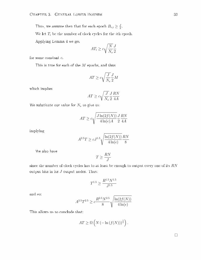
Chapter 3. General Lower Bounds 33
Thus, we assume then that for each epoch Br,i ≥ J2.
We let Ti be the number of clock cycles for the ith epoch.
Applying Lemma 4 we get
ATi ≥ c
√N
Ns
J
2
for some constant c.
This is true for each of the M epochs, and thus
AT ≥ c
√J
Ns
J
2M
which implies
AT ≥ c
√J
Ns
J
2
RN
4A
We substitute our value for Ns to give us:
AT ≥ c
√J ln(2f(N))
4 ln(ε)A
J
2
RN
4A
implying
A2.5T ≥ cJ1.5
√ln(2f(N))
4 ln(ε)
RN
8
We also have
T ≥ RN
J
since the number of clock cycles has to at least be enough to output every one of its RN
output bits in its J output nodes. Thus:
T 1.5 ≥ R1.5N1.5
J1.5
and so:
A2.5T 2.5 ≥ cR2.5N2.5
8
√ln(2f(N))
4 ln(ε)
This allows us to conclude that:
AT ≥ Ω(N (− ln (f(N)))
15
).

Chapter 3. General Lower Bounds 34
3.6 Encoder Lower Bounds
In terms of scaling rules, all the decoder lower bounds presented herein can be extended
to encoder lower bounds. The main structure of the decoder lower bounds (inspired
by [2, 5]) involves dividing the circuit into a certain number of subcircuits. Then, we
argue that if the bits communicated within the circuit is lower, then there must be one
subcircuit where the bits communicated to it are less than the bits it is responsible for
decoding. If all the inputs bits in that circuit are erased, the decoder must make an error
with probability at least 1/2.
In the encoder case, we also take inspiration from [2,5]. In this case, the N outputs of
the encoder circuit can be divided into a certain number of subcircuits. Then we consider
the bits communicated out of each subcircuit. This quantity must be proportional to the
number of output bits in each subcircuit. Otherwise, there will be at least one subcircuit
where the number of bits communicated out is less than the number of output nodes in
the subcircuit. Call these bits that were not fully communicated out of this subcircuit
Q. Suppose that once the output bits of the encoder are injected into the channel, all
the bits in Q are erased. Now, the decoder must use the other bits of the code to decode.
But, the subcircuit containing Q in the encoder communicated less than |Q| bits to the
other outputs of the encoder. By directly applying Lemma 1, we see that no matter what
function the decoder computes, it must make an error with probability at least 1/2. An
argument of this structure and following exactly the structure of Theorems 1, 2, 3, 4,
and 11 for the decoders gives us the following theorems, whose proofs are omitted.
Theorem 5. All fully-parallel f(N)-encoding schemes with number of clock cycles T (N)
have energy
E(N) ≥ Ω
(−N log(f(N))
T (N)
)
with optimal lower bound of E ≥ Ω(N√− log f(N)
)when T (N) ≥
√− log(f(N)).
All serial, f(N)-encoding schemes have energy that scales as
E(N) ≥ Ω (−N log f(N)) .
All increasing output node, output-regular f(N)-encoding schemes have energy that scales
as
E(N) ≥ Ω(N(− log (f(N)))1/5
).

Chapter 3. General Lower Bounds 35
3.7 Asymptotic Probability of Error Approaching a
Constant
In this chapter, we discuss f(N)-coding schemes where f(N) approaches 0 as N increases.
However, our analysis does not quite extend to coding schemes in which error probability
approaches a constant, and not 0. In Appendix A.1 we analyze the corner case and show
that schemes with asymptotic error probability less than 1/2 have energy that scales as
(1) Ω(N√
logN) for fully parallel decoders, (2) Ω(N logN) for serial decoders, and (3)
Ω(N log1/5(N)) for increasing-output node output-regular decoders. The proofs use a
similar approach to the proofs of this chapter.
The fundamental prob-
lem of communication is
that of reproducing at one
point either exactly or ap-
proximately a message se-
lected at another point.
Claude Shannon
4LDPC Codes
In the previous chapter, we derived lower bounds on the energy complexity of general
encoding and decoding circuits. In this chapter, we consider the VLSI energy complexity
of low-density parity-check (LDPC) codes, an important family of error control codes
introduced by Gallager [43]. The complexity of LDPC decoder circuits depends on the
complexity of their underlying Tanner graph, which is often generated randomly in their
theoretical analysis. Thus, the scaling rules we derive in this chapter are of an almost
sure variety: that is, they are true for codes with a Tanner graphs that are in a set of
Tanner graphs with probability approaching 1. We derive tight upper bounds for the
energy complexity of directly-implemented Tanner graphs in this chapter, but defer the
discussion regarding upper bounds for serial LDPC decoders to Chapter 6.
The rst result of this chapter is an almost-sure scaling rule for the energy com-
plexity of LDPC decoders. In particular, we analyze ensembles generated according to
a uniform conguration distribution (see Denition 36). We show, subject to some mild
conditions, that the minimum bisection width of a randomly generated bipartite cong-
uration asymptotically almost surely has minimum bisection width proportional to the
number of vertices. This implies an Ω(N2/d2max) lower bound on the energy of directly-
implemented LDPC decoders (see Denition 24) and a Ω(N3/2/dmax) lower bound on the
energy of serialized decoders (see Denition 33).
36

Chapter 4. LDPC Codes 37
We also show that a capacity-approaching sequence of non-split-node directly-implemented
LDPC decoders (see Denition 27 must have energy that scales as Ω(χ2 ln3(χ)), where
χ = (1 − R/C)−1 is the reciprocal gap to capacity, where R is the code rate and C the
capacity of the channel over which the code is transmitted. This lower bound contrasts
with the universal lower bound of Ω(χ2√
ln(χ)) of [42].
The Ω(χ2ln3(χ)) result applies to decoding circuits where messages are passed on
a Tanner graph induced by a parity check matrix of the underlying code. This lower
bound does not apply to decoding algorithms that use modied Tanner graphs with
punctured variable nodes like those used for the non-systematic irregular repeat accumu-
late (IRA) codes of [44] or the compound low-density generator matrix (LDGM) codes
of [45]. However, computations show that the Ω(N2/d2max) and Ω(N3/2/dmax) almost sure
lower bounds apply to the non-systematic IRA construction of [44] for many parameters.
We begin the chapter in Section 4.1 with a discussion of prior related work. In
Section 4.2 we dene directly-implemented LDPC decoders and in Section 4.3 we dene
serialized LDPC decoders. In Section 4.4, after dening some properties of node-degree
lists, we present the main theorem. We proceed to show how this theorem allows us
to nd scaling laws for the energy of LDPC decoders in Section 4.5. In Section 4.6 we
derive a Ω(χ2 ln3 χ
)scaling rule for capacity-approaching sequences of non-split-node
LDPC decoders.
4.1 Prior Work
4.1.1 Related Work on Circuit Complexity and LDPC codes
The work in [46] provides a discussion of techniques used to minimize energy consumption
in LDPC decoder circuit implementations. In contrast to this work, the results in this
chapter provide a theoretical asymptotic analysis of energy.
In [47], the authors assume that the average wire length in a VLSI instantiation of
a Tanner graph is proportional to the longest wire, and that the length of the longest
wire is proportional to the diagonal of the circuit upon which the LDPC decoder is
laid out. The implication of these assumptions is an Ω (N2) scaling rule for the area
of directly-implemented LDPC decoders, which is the same result as Corollary 4 of this
chapter. However, these assumption are taken as axioms without being fully justied;
there certainly can exist bipartite Tanner graphs that can be instantiated in a circuit
without such area. We show that, in fact, the Ω (N2) scaling rule is justied for almost
all directly-implemented Tanner graphs (so long as some mild conditions are satised).

Chapter 4. LDPC Codes 38
More recently, Ganesan et al. [48] analyze the VLSI complexity of certain classes of
LDPC decoding algorithms, including analyzing how the number of iterations required
for such algorithms scales with block error probability. Moreover, the authors show
that a judicious choice of node degree distributions can optimize the total (transmit +
decoding) power for coded communication using LDPC codes by simulating real circuits
and their code performance. The Ganesan et al. paper complements this chapter; we do
not analyze how the number of iterations depends on target block error probability, nor
do we simulate any actual circuit performance. Neither the Ganesan et al. paper nor
this chapter consider the performance of LDPC codes whose interconnection complexity,
and not just degree distribution, is optimized.
4.1.2 Related Work on Graph Theory
We use a combinatorial approach to derive our almost sure lower bounds on the minimum
bisection width of randomly generated conguration. This contrasts with a common
approach that considers a graph's Laplacian (See Denition 8.6.15 in [49]). Fiedler [50],
shows that the second largest eigenvalue of a graph's Laplacian, λ2, can be used to nd
a lower bound of λ2N4
on the graph's minimum bisection width. In [51], the authors nd
some bounds on the bisection width of graphs that are related to this λ2 value. The
authors in [52] provide almost sure upper bounds for the bisection width of randomly
generated regular graphs. Luczak et al. [53] also study the minimum bisection width
of graphs generated according to a distribution dierent from ours. Furthermore, our
analysis is of random bipartite graphs, as opposed to random regular graphs. As well, our
result makes only weak assumptions on the node degree distribution, without requiring
a degree-regularity assumption, in contrast to previous work.
4.2 Directly-Implemented LDPC Decoders
The main result of this chapter involves the minimum bisection width (MBW) of a
randomly generated bipartite graph (See Denition 2). For a graph G = (VG, EG) and a
subset of vertices V ′ ⊆ VG, we let φG(V ′) denote the minimum bisection width of V ′ in
G.
LDPC codes are linear codes rst studied by Gallager in [43]. Given a parity-check
matrix H withM rows for a code of length N , the Tanner graph of H is a bipartite graph
where one part of the graph contains N vertices called variable nodes and the other part
is composed of M check nodes. Each check node is associated with a row of the parity

Chapter 4. LDPC Codes 39
check matrix and each variable node with a column. A check node is connected to a
variable node if and only if the row associated with the check node has a 1 in the column
corresponding to the variable node.
Since there are many possible parity-check matrices for a given linear code, there are
many possible Tanner graphs associated with that code. An LDPC decoding algorithm
for a code is a message-passing procedure where messages are passed over the edges of a
particular Tanner graph of the code.
We consider two possible paradigms to implement LDPC decoding algorithms with a
circuit: a directly-implemented and a serialized technique. To be precise, we will use the
following graph-theoretic terminology.
Denition 21. [49] (Denition 2.2.7) The contraction of an edge e connecting vertices
u and v is the removal of e and the replacement of u and v with a vertex whose incident
edges are the same edges incident on u and v, except of course e.
Denition 22. The reverse of edge contraction is vertex splitting. This is a process that
replaces a vertex v with two vertices v1 and v2 with an edge between them. For every
edge incident on v there is exactly one edge either connecting to v1 or to v2. We say that
v1 and v2 are split from vertex v.
Denition 23. [49, Denition 6.2.13] A graph G is a minor of a graph G′ if the graph
G can be obtained by deleting vertices and edges of G′ and contracting edges of G′. We
say in this case that G′ contains G as a minor. Equivalently, G′ contains G as a minor
if there is a sequence of vertex splits of G that results in a subgraph of G′.
Denition 24. A circuit is a directly-implemented LDPC decoder associated with an
LDPC code with a Tanner graph T if its graph contains T as a minor.
Denition 24 allows Tanner graph computational nodes to be split and thus logic
gates associated with the computation for a single check or variable nodes can appear in
dierent parts of the circuit.
Denition 25. Let G′ be obtained by successively splitting the vertices of a graph G
with labelled vertices. When a labelled vertex is split, move the label arbitrarily to one
of the new vertices. The labelled vertices of G′ we term the vertices of G′ corresponding
to G, or the G-corresponding vertices.
Denition 26. Let G′ be obtained by successively splitting the vertices of a graph G.
Consider a vertex v in the graph G. Then its v-descendants in G′ are those vertices that
were originally v, or split from v, or split from a vertex that was split from v, and so on.

Chapter 4. LDPC Codes 40
Consider a labelling of the G-corresponding vertices of G′. A particular labeled vertex v
is considered the parent of all those vertices descended from the vertex of G from which
v descended.
Denition 27. Consider a circuit which contains Tanner graph T as a minor. Consider
each set of vertices descended from a vertex in T . If the wires connecting these vertices do
not cross any other wires in the circuit, then such a circuit is said to be a non-split-node
directly-implemented LDPC decoder.
Lemma 5. Let v be a G-corresponding vertex of G′, where G′ is obtained from G by
vertex splitting. Then the number of edges leading from the descendants of v to the rest
of the graph is not more than dmax (in fact, not more than the degree of the original
vertex).
Proof. This is easily observed by drawing a circle around a node and then successively
splitting this vertex. The number of edges exiting the circle does not increase as the
vertices are split.
Denition 28. We let Amin(G) be the minimum circuit area of a circuit whose associated
graph is G.
Let G′ be a graph obtained by vertex splitting G. We let V ′G be the G-corresponding
vertices of G′ so that φG′(V′G) is the minimum bisection width of the G-corresponding
vertices of G′. This is of course dependent on how the nodes are labeled during the
splitting process. Thus to be more precise this represents the smallest MBW of the
nodes corresponding to G over all labellings.
The graph for a directly-implemented LDPC decoder is obtained by vertex splitting
and adding edges and vertices to the original Tanner graph. Adding edges and vertices
cannot decrease the MBW of V ′G, but vertex splitting might. However, vertex splitting
can only decrease the MBW of V ′G by a limited amount, as the following lemma proves.
Lemma 6. If G′ is obtained by a sequence of vertex splits of a graph G = (VG, EG) with
no isolated vertices, and G has maximum node degree dmax(G), then
φG′(V′G) ≥ φG(VG)
dmax(G) + 1≥ φG(VG)
2dmax(G).
Proof. Suppose not, i.e., that φG′(V′G) < φ(G)
1+dmax(G). Note that G can be obtained by
contracting the vertices of G′. Consider a minimum bisection of the G-corresponding
vertices of G′, and place one side of the bisection on the left side and the other the right

Chapter 4. LDPC Codes 41
side. There will be some vertices on the left side that are descended from vertices on the
right side, and vice versa. We call such vertices bisection-crossing descendants.
If such a bisection of V ′G has ω′ edges crossing it, then there are at most ω′ G-
corresponding vertices ofG′ that have bisection-crossing descendants. To see this, observe
that the set of descendants of a vertex must be connected by paths using only their
vertices, so there must be at least one unique edge crossing the bisection for each G-
corresponding vertex of G′ that has a bisection-crossing descendant.
We shall now show how to construct a bisection of G with at most ω′(1 + dmax(G))
edges. Simply move all the bisection-crossing descendants of G to the side of their parent,
while keeping the G-corresponding vertices of G′ on the same side of the bisection. Then,
contract all the vertices that were split in obtaining G′ from G. By Lemma 5, for
each H-corresponding vertex of G, we observe that at most dmax edges will connect the
descendants of v to vertices on the opposite side of the bisection. Thus, moving the
vertices to the side of their descendant can at most add ω′dmax(G) edges crossing the
bisection, and the resulting bisection has width at most ω′ + ω′dmax
Thus, we have constructed a bisection ofG of width less than φG(VG)1+dmax(G)
(1 + dmax(G)) =
φG(VG), a contradiction.
Note that if a graph G′′ contains G as a minor, then it contains a subgraph G′ that
is obtained by a sequence of vertex splits of G. This allows us to conclude:
Lemma 7. If a graph G′′ contains a graph G = (VG, EG) as a minor, then the minimum
bisection width of the nodes of G′ corresponding to G is at least φG(VG)/(1 + dmax(G)).
Thus, by applying Lemma 2, the circuit area of G′′ is at least
Amin(G′′) ≥ φ2G(VG)
4(1 + dmax(G))2≥ φ2
G(VG)
16d2max(G)
4.3 Serialized LDPC Decoders
Not all LDPC decoders are directly-implemented. This motivates considering a more
general class of LDPC decoder. Our denition of a serialized circuit includes both serial-
ization of the message-passing step (for example, by introducing an interleaver that works
over multiple clock cycles to pass messages from node to node), and serializing compu-
tation steps (by having one computational node perform the computation for multiple
check or variable nodes, but at dierent clock cycles). The key idea is that a serialized
circuit simulates a joined Tanner graph, which we will dene in this section.
To do so we rst dene a computation's communication multi-graph.

Chapter 4. LDPC Codes 42
Denition 29. The communication directed multigraph, or communication graph for a
circuit operated for T clock cycles is the graph obtained by replacing each computational
node with a vertex and replacing each wire between two computational nodes (u and v,
say) with 2T edges, T of them directed from u to v and T of them directed from v to u.
We place 2 edges per wire because we assume, for the purpose of lower bound, that a bit
is communicated in both directions each clock cycle.
Denition 30. Two unconnected vertices v1 and v2 of a graph can be joined by removing
the two vertices and replacing them with a single vertex v. Each edge connecting v1 or
v2 to a vertex (denoted a) in the original graph is replaced with an edge connecting v to
a.
Denition 31. A graph obtained by rst splitting the nodes of a Tanner graph T and
then joining nodes that are not associated with variable node inputs is a joined Tanner
graph obtained from T .
For a joined Tanner graph T ′, we let jmax(T ′) be the maximum number of vertices
joined to form a single vertex. Often its dependence on T ′ will be suppressed.
Denition 32. A communication graph Gcomm simulates a graph G if there is a subset
of vertices of Gcomm in a one-to-one correspondence with the vertices of G, and for each
edge in G, there is a path connecting the two corresponding vertices in Gcomm. Moreover,
these paths are mutually edge-disjoint.
We can now dene a serialized LDPC decoder.
Denition 33. A serialized LDPC decoder for a Tanner graph T is a circuit that simu-
lates a joined Tanner graph obtained from T during each iteration.
Note that if a particular node of such a circuit corresponds to a vertex formed by
joining j nodes then there must be at least j clock cycles performed each iteration.
In the sections that follow, we prove an Ω(N2/d2max) scaling rule for the energy of
directly-implemented LDPC decoder circuits in Corollary 4 and an Ω(N3/2/dmax) lower
bound for serialized LDPC decoders in Theorem 7.
4.4 Almost Sure Scaling Rule
Our main theorem is fundamentally graph-theoretic in nature and applies to graphs
generated according to a standard uniform random conguration distribution.

Chapter 4. LDPC Codes 43
Denition 34. Consider the set of bipartite graphs G = (VL t VR, EG) (where the
symbol t is the disjoint union symbol) in which |VL| = N , |VR| = M . Let VL be called
the left nodes and VR the right nodes. Order the left nodes and right nodes in terms of
increasing node degree. Let li be the degree of the ith left node in the graph, and let ri be
the degree of the ith right node in the graph. Then we say that L = (l1, l2, . . . , lN) ∈ (N)N
is the left node degree list and R = (r1, r2, . . . , rM) ∈ (N)M the right node degree list.
Note that the node degree lists are non-standard; often it is the node degree distri-
bution that is considered. However, in Appendix A.2 we show how to present our results
in terms of the more standard node degree distributions.
Given a list Z = z1, z2, . . . , zN with z1 ≤ z2 ≤ . . . ≤ zN , we dene
Stop (Z) =N∑
i=bN2 czi. (4.1)
Note that implicitly this function takes as input the size of the input vector. This is the
sum of the half of the elements of the list with the greatest value.
Denote the set of bipartite graphs with left and right node degree lists L and R as
G(L,R). Note that the number of edges in each particular graph in G(L,R) is |EG| =∑Ni=1 li =
∑Mi=1 ri.
For convenience of counting, we will consider not the set of graphs with a particular
degree list, but rather the set of congurations with this degree list. We can associate
each node in a graph with a number of sockets equal to its degree. This node and socket
conguration model is a standard way to consider the set of bipartite graphs that form
the Tanner graphs of LDPC ensembles, and in particular is discussed thoroughly in [54].
Denition 35. A set of left nodes and right nodes with an ordered labeling of the sockets
of each node, together with a permutation mapping the left node sockets to the right
node sockets is called a conguration.
Let the set of congurations with node degree lists L and R be denoted B (L,R).
Clearly, |B (L,R) | = |EG|!. Since a conguration is merely a graph with a labeling
of sockets for each node, graph properties, including minimum bisection width, can be
extended to describe congurations in the natural way.
Denition 36. The uniform conguration distribution for xed node degree lists is the
probability distribution in which the probability of each conguration with these node
degree lists has uniform probability.

Chapter 4. LDPC Codes 44
Let
Ba = G ∈ B (L,R) : ∃ a bisection KG ⊆ EG such that |KG| = a
be the set of congurations that have a bisection of size a. Note that Ba does not represent
the set of congurations in B (L,R) with minimum bisection width a, but rather the set
of congurations with some bisection of size a.
Let B∗a be the set of congurations in B (L,R) that have a bisection of size a or less,
i.e.,
B∗a =a⋃
i=0
Bi.
Given a left node node degree list L of length N and right node degree list R of length
M , where L and R are ordered by increasing degree and M ≤ N , we dene
δ (L,R) =max (Stop (L) , Stop (R))
N(4.2)
We also let
σ (L,R) =|EG|N− δ (L,R) . (4.3)
For notational convenience we will abbreviate these two quantities as δ and σ and
their dependence on the node degree distribution under discussion is to be implicit. Note
that |EG| = δN + σN .
Consider a conguration with left degree list L and right degree list R. For a given
subset of vertices V ′ we can divide this set into two disjoint sets, V ′L = V ′ ∩ VL and
V ′R = V ′ ∩ VR. Let Sleft (V ′) =∑
v∈V ′Ldeg (v) and Sright (V ′) =
∑v∈V ′R
deg (v) denote the
number of left and right sockets in V ′, respectively.
Lemma 8. For any bipartite conguration G = (VL t VR, EG) with left degree list L and
right degree list R, where |VL| = N and |VR| = M , for any collection V ′ of N+M2
vertices,
min (Sleft(NV ), Sright(NV )) ≤ Nδ.
Proof. Suppose not. This implies that both Sleft(V′) > Nδ and Sright(V
′) > Nδ. Divide
the vertices in V ′ into the left nodes V ′L and right nodes V ′R. It must be that |V ′L|+ |V ′R| =N+M
2. Thus, it must be that |V ′L| ≤ N
2or |V ′R| ≤ M
2(otherwise their sum would exceed
M+N2
). Let us consider the case in which |V ′L| ≤ N2(the other case leads to an analogous
argument). If |V ′L| ≤ N2and Sleft(V
′) > Nδ then, in particular Sleft (V ′) > Stop(L). But
Stop(L) by (4.1) is the sum of the highest degree left nodes. A collection of at most half
these nodes cannot exceed this quantity, leading to a contradiction.

Chapter 4. LDPC Codes 45
We will need the following lemma for our proof:
Lemma 9. The quantity m!n!, subject to the conditions 0 ≤ n ≤ m ≤ Z ≤ m + n ≤ Y
and that Y , Z, m and n are all integers cannot exceed Z!(Y − Z)!.
Proof. See Appendix A.3.
We can now give the main technical lemma of this chapter, which states that the
set of congurations with a small bisection is small, which will imply that with high
probability a Tanner graph has MBW proportional to N .
Lemma 10. If a conguration G = (VL t VR, EG) with |VL| = N and with degree lists L
and R is generated according to the uniform conguration distribution, then the probability
that this conguration is in the set B∗a when
0 ≤ a ≤ σ(L,R)N (4.4)
is upper bounded by
P (B∗a) ≤(a+ 1)N2
(NN2
)2(|EG|a
)4a! (δ(L,R)N)! (σ(L,R)N − a)!
(δ(L,R)N + σ(L,R)N)!. (4.5)
Proof. This follows from a counting upper-bounding argument, where the key idea is to
over-count a set of objects that is larger than B∗a, namely the set of quadrant congura-
tions with a bisection of size a or less.
Let the set of congurations in B (L,R) having a bisection of size a be denoted by
Ba. Then we can say that, according to the uniform conguration distribution, the
probability of the event of generating a conguration with a bisection of size a is given
by:
P (Ba) =|Ba||EG|!
,
recalling that |EG| is the number of edges in the congurations of B (L,R).
We will now bound the number of congurations in B (Λ, P ) with a bisection of size
a, and we will assume that a < σN . To do so, we will dene a quadrant conguration,
show that the number of quadrant congurations with a bisection of size a is greater
than or equal to Ba, and then upper bound the number of quadrant congurations with
a bisection of size a or less.
A quadrant conguration of a bipartite conguration G = (VL t VR, EG) is an ordered-
tuple Q = (G, TL, TR, BL, BR) where the vertices are divided into 4 disjoint sets, the top

Chapter 4. LDPC Codes 46
Figure 4.1: An example of a particular quadrant conguration associated with a leftnode degree list L in which all the nodes have 2 sockets and a right node degree listR = (2, 3, 4, 4, 5). The number of left nodes N = 9 and the number of right nodesM = 5. The conguration drawn is a quadrant conguration in Q4,1
3 for the particulardegree lists. Recall that the superscript denotes that there are i = 4 top left nodes andj = 1 edges leading from top left nodes to bottom right nodes. The subscript indicatesthat there are a = 3 edges between top and bottom vertices. The edges forming thebisection are solid lines. The horizontal dotted line indicates where the bisection occurs.

Chapter 4. LDPC Codes 47
left nodes (TL), the top right nodes (TR), the bottom left nodes (BL), and the bottom
right nodes (BR), in which TL, BL ⊆ VL, TR, BR ⊆ VR and ||TR ∪ TL| − |BR ∪BL|| ≤ 1.
Vertices in TL and TR are considered to be top nodes or and similarly for the bottom
nodes.
Note that every bipartite graph has at least one quadrant conguration induced by
arbitrarily dividing the vertices in half, and denoting one half of these vertices top nodes
and the other half bottom nodes. Thus, the set of quadrant congurations with a par-
ticular degree distribution is at least as big as the set of congurations with a particular
degree distribution. Because a quadrant conguration Q = (G, TL, TR, BL, BR) contains
a graph G, graph properties can be extended to describe a quadrant conguration.
Denote the set of quadrant congurations with set node degree lists L and R in which
a is the number of edges connecting top nodes to bottom nodes as Qa. Note that the
dependence of Qa on a particular node degree distribution is implicit. Observe that every
conguration with a bisection of size a has a corresponding quadrant conguration in Qa
created in the natural way by denoting one bisected set of vertices as the top nodes, and
the other the bottom nodes. Thus |Ba| ≤ |Qa|.
For ease of discussion, we will assume that the total number of nodes M + N in the
set of congurations under discussion is even, so that M+N2
is an integer.
Denote the set of quadrant congurations in Qa in which there are i top left nodes
and j edges connecting top left nodes to the bottom right by Qi,ja . This of course implies
that there are M+N2− i top right nodes and a− j edges leading from the bottom left to
the top right nodes. We can see in Figure 4.1 an example of such an element that we are
counting for the case of N = 8 and a = 4, i = 4 and j = 2. Note then that
Qa =N⋃
i=0
a⋃
j=0
Qi,ja .
We bound the size of Qi,ja by counting all quadrant congurations with a bisection of
size a that are the edges connecting top nodes to bottom nodes. In the following, for

Chapter 4. LDPC Codes 48
compactness, we let δ = δ(L,R) and σ = σ(L,R). We have
∣∣Qi,ja
∣∣ ≤(N
i
)
︸ ︷︷ ︸a
(M
M+N2− i
)
︸ ︷︷ ︸b
·(|EG|
j
)(|EG|j
)( |EG|a− j
)( |EG|a− j
)
︸ ︷︷ ︸c
·(j)! (a− j)!︸ ︷︷ ︸d
(δN)! (σN − a)!︸ ︷︷ ︸e
, (4.6)
where
a. Represents a choice of i top left nodes.
b. Represents a choice of M+N2− i top right nodes.
c. The quantity(|EG|
j
)is an upper bound on the number of choices of j sockets that
will have edges that cross the bisection line chosen from the top variable nodes, and(|EG|j
)is an upper bound on the number of choices for the bottom right sockets to which
these edges will be connected. For a conguration in Bi,ja there must also be a− j edges
leading from the bottom left to the top right. The quantity(|EG|a−j
)is an upper bound
on the number of choices of sockets in the bottom left that can have edges crossing the
middle bisection, and similarly(|EG|a−j
)is an upper bound on the number of choices for the
sockets connected in the top right.
d. Counts the number of permutations of edges that join the top half to the bottom
half (rst counting the j connections from the top left nodes to the bottom right nodes,
then the a− j connections from the bottom left nodes to the top right nodes).
e. This step involves permuting the connections of the remaining sockets in the
top half and the bottom half. However, at this point it is not clear how many sockets
are in the top half or the bottom half. However, we can upper bound the number of
permutations possible. The number of sockets available in the top left nodes must equal
the number of sockets available in the top right nodes (because in order to construct a
valid conguration this must be true). By construction, the total number of nodes in the
top left and top right is M+N2
, and thus the number of sockets available cannot exceed
δN , by Lemma 8. Suppose the number of sockets available for all the top left nodes is
Ms and the sockets available in the bottom left nodes is Ns. Then there are at most
Ms!Ns! ways to permute these. We also know that Ms + Ns = |EG| − a (since the total
number of sockets available on one side of the constructed quadrant conguration is |EG|and a have been used to cross between top nodes and bottom nodes), and that Ms ≤ δN

Chapter 4. LDPC Codes 49
and Ns ≤ δN . Subject to these restrictions, a direct application of Lemma 9 implies
Ms!Ns! ≤ (δN)! (|EG| − δN − a)! = (δN)! (σN − a)!
The proof mostly follows from simplication of these bounds and the details of the
rest of the proof are given in Appendix A.4.
Consider a sequence of random congurations G1, G2, . . . where each Gi in the se-
quence is a conguration generated according to the uniform conguration distribution,
in which the ith conguration is drawn according to node degree lists Li and Ri. Note
that the randomness for each element of such a sequence does not come from the degree
lists: we are assuming that these lists are xed. It is the interconnections between nodes
that is random. We specically concern ourselves with a sequence in which the number
of left nodes N increases without bound. For such a sequence, denote the number of
left nodes of the ith conguration as Ni. We will abbreviate the quantities δ (Li, Ri) and
σ (Li, Ri) with the symbols δi and σi respectively (see lines (4.2) and (4.3). We let B∗a,ibe the set of congurations with node degree lists (Li, Ri) with a bisection of size a or
less.
Theorem 6. Consider a sequence of right and left node degree lists (Li, Ri), and a
sequence bipartite congurations Gi where Gi is generated according to the random con-
guration distribution with node degree list (Li, Ri). If
lim supi→∞
[2 ln(2) + δi
(ln
(δi
δi + σi
))+
σi
(ln
(σi
δi + σi
))]< 0 (4.7)
then there exists some β > 0 in which
limi→∞
P(Gi ∈ B∗βNi,i
)→ 0
where Gi ∈ B∗βNi,i is the event that the ith conguration has a bisection of size βNi or
less. In particular, this is true for any 0 < β < σ that satises:
limi→∞
2 ln(2) + 4H(
β
δi + σi
)+ β
(ln
(β
σi − β
))
+δi
(ln
(δi
δi + σi
))+ σi
(ln
(σi − βδi + σi
))< 0. (4.8)
Remark 3. Stated less precisely, this theorem says that in the limit, a random bipartite
conguration will, with high probability, have no small bisections.

Chapter 4. LDPC Codes 50
Proof. This proof involves algebraic manipulation of the expression in Lemma 10 and
showing that if the conditions of the theorem are satised, the limit evaluates to 0. The
details of this computation are given in Appendix A.5.
In the corollaries that follow, we consider a sequence of congurations generated
according to the uniform conguration distribution. Let φi be the minimum bisection
width of the ith conguration. Note that this symbol is a random variable. Theorem 6
now has an obvious corollary.
Corollary 3. If there is a sequence of congurations as described in Theorem 6, in which
the condition in (4.7) is satised then limi→∞ P (φi ≥ βNi) = 1 for some β > 0.
Proof. Note that B∗a is the event that a random conguration has a bisection of size a
or less. The complement of this event is the event that a random conguration has no
bisection of size a or less, and thus equal to the event that a random conguration has
minimum bisection width greater than or equal to a. The corollary ows directly from
this observation.
Remark 4. This Corollary and the results that follow can be slightly strengthened, be-
cause we know that the probability that a bisection exists with size less than βN ap-
proaches 0 exponentially quickly. Let Iφi/Ni<β be the event that the graph with Ni left
nodes has a bisection less than βN . We easily observe that∑
n P (φi/Ni > β) <∞ and
so by the Borel-Cantelli Lemma [55,56], the probability that a bisection of size less than
βNi occurs innitely often is 0. Thus, P (lim infi→∞ φi/Ni ≥ β) = 1 for some β > 0.
4.5 Almost Sure Bounds on Suciently High Rate LDPC
Decoder Circuits
To apply our results to LDPC decoder circuits, we rst dene a few terms in order to
make our claims precise.
Denition 37. [57] For a given parity check matrix H for a code of block length N and
rate R, we dene ∆(H) as the number of 1s in the matrix divided by NR, and call this
quantity the density of the matrix H.
Denition 38. For a code of rate R associated with a channel with capacity C, let
χ = (1−R/C)−1 be the reciprocal gap to capacity.

Chapter 4. LDPC Codes 51
Denition 39. Consider a sequence of codes and decoders for a particular channel. We
let the block error probability of the ith code in the sequence be Pe,i. Then such a
sequence is vanishing-error-probability if limi→∞ Pe,i = 0.
The following result, which is a simple implication of Sason and Urbanke [57] which
we present using our notation shows that as capacity is approached the density of a code's
parity check matrix must approach innity. We will use this result in Corollary 4 and
Theorem 8.
Lemma 11. [57, Theorem 2.1] Consider a sequence of parity check matrices Hi fora channel with capacity C. Let χi denote the reciprocal gap to capacity of the ith code.
Let the density of the ith parity matrix be ∆(Hi). Suppose that there is a decoder for each
of these codes, and thus each code for matrix Hi has an associated block error probability
(Pe,i). Suppose as well that in the limit of increasing i Pe,i approaches 0. Then, there is
some constant K1 such that, for suciently large i,
∆(Hi) > K1 ln (χi) .
4.5.1 Energy Complexity of Directly-Implemented LDPC De-
coders
Corollary 4. Consider a vanishing-error-probability LDPC coding scheme where each
code in the scheme is generated according to a uniform conguration distribution. Suppose
that each decoder in the scheme is a directly-implemented LDPC decoder. If such a scheme
has asymptotic rate suciently close to capacity, then for this scheme
limi→∞
P(Ai ≥ cN2
i /d2max
)= 1
for some constant c > 0, where dmax is the maximum node degree (possibly a function of
N). Energy is bounded similarly.
Proof. Note that Lemma 11 implies that as rate approaches capacity, the parity-check
matrix density must approach innity. But this implies that the associated Tanner graph
has number of edges per node approach innity. Then obviously the quantity δ must
approach innity. We can use this observation that for codes of sucient closeness to
capacity the expression
2 ln(2)− (δ + σ)H(
δ
δ + σ
)< 0 (4.9)
must be satised.

Chapter 4. LDPC Codes 52
To see this, note that δ approaches∞ for a capacity-approaching code. What happens
to σ is either (a) limN→∞δ
δ+σ< 1 or (b) limN→∞
δδ+σ
= 1, or (c) this limit does not exist.
Note that this value cannot exceed 1 because necessarily σ ≤ δ.
In the case of (c), it must be that the value of σ alternates and no limit can be dened.
In this case, however, we should consider the specic subsequence of decoders in which
either (a) or (b) applies. It will be clear that since for each subsequence the appropriate
scaling rule holds, thus it must be true for the entire sequence.
In case (a): in the limit, ln(
δδ+σ
)< 0 and so δ
(ln(
δδ+σ
))→ −∞, as δ approaches
∞. Since σ(ln(
σδ+σ
))< 0 in any case (a consequence of σ ≤ δ), thus in the limit the
inequality (4.9) will be satised.
For case (b), in which ln(
σδ+σ
)→ −∞, note that σ is positive, so σ
(ln(
σδ+σ
))→ −∞
, and thus in the limit (4.9) will also be satised.
If the scheme has asymptotic rate suciently close to capacity, then for suciently
large block lengths in this scheme the node degree list satises the sucient condition of
Theorem 6, and the code's Tanner graph has MBW at least βNi for some β > 0 with
probability approaching 1. In this case, the decoder, which contains a subgraph obtained
by splitting the vertices of the Tanner graph, but have MBW at least βNi/(2dmax) by
Lemma 6. In this case, Lemma 7 implies Ai ≥ (βNi)2 /(16d2
max) and thus:
limi→∞
P
(Ai ≥
(βNi)2
16d2max
)= 1
as expressed in the theorem statement. A similar bound is obviously then true for the
energy per iteration of such circuits.
4.5.2 Serialized Decoders
In this section we generalize our results to serialized circuits. To develop this theory,
however, we need to dene some new terminology. In particular, we will generalize the
notion of minimum bisection width by considering collections of bipartitions of the nodes
of a graph.
Denition 40. A bipartition of a set X is the partition of the set into two disjoint sets
X1 and X \X1.
We will represent a bipartition by a single set contained within it.

Chapter 4. LDPC Codes 53
Denition 41. Given a set of vertices VF of a graph G, a bisection of VG is a bipartition
of VG into V1 and V2 such that ||V1| − |V2|| ≤ 1.
We see that a bisection is an example of a bipartition. What we will be interested
in is collections of bipartitions that are zig-zaggable. It is the zig-zaggable property of
the bisections of a graph that allows Thompson to prove in [1] that A ≥ φ2G(VG)/4 for a
circuit with graph G = (VG, EG) with MBW φG(VG).
Denition 42. Let X be a nonempty nite set. If ∅ ⊆ A ⊂ B ⊆ X, a simple chain from
A to B is a sequence S1 ⊂ S2 ⊂ . . . ⊂ SL with S1 = A and SL = B and |Si+1 \ Si| = 1
for i = 1, 2, . . . , L− 1.
Consider a subset (denoted C) of the bipartitions of a set X.
Denition 43. A subset of the bipartitions of a set X is zig-zaggable if the following
conditions hold:
1. All simple chains from ∅ to X contain an element of C.
2. If A and B are subsets of X such that A ⊆ B, and there is a set D in C such that
A ⊆ D ⊆ B, then all simple chains from A to B contain an element of C.
Lemma 12. The collection of bisections of a set are zig-zaggable.
Proof. A set C induces a bisection of X if an only if |C| = b|X|/2c or |C| = d|X|/2e. Asimple chain from ∅ to X results in a sequence of bipartitions where the size of one of
the sets of the bipartitions increases by 1 each time. One of these bipartitions must thus
be a bisection. For property 2, suppose that a simple chain from A to B contains a set
C that induces a bisection. Then, either A or B are bisections, or they are not and then
|A| < b|X|/2c and |B| > d|X|/2e, and then any simple chain from A to B will include a
bisection.
We will show however that a more general collection of bipartitions is zig-zaggable.
Denition 44. The width of a bipartition of a set of vertices of a graph is the number
of edges connecting the vertices between the two sets of the bipartition.
Denition 45. The C-bipartition width of a graph with respect to a collection of bipar-
titions C is the minimum width of all bipartitions in C.
Using the denition of zig-zaggable (Denition 43), we can now easily adapt Thomp-
son's proof [1] and derive the following lemma:

Chapter 4. LDPC Codes 54
Lemma 13. Let C be a zig-zaggable collection of bipartitions of a graph G, and let ωC be
the C-bipartition width of the graph. Then,
Amin(G) ≥ ω2C
4.
Proof. A detailed proof is given in Appendix A.6 that essentially follows the proof of
Thompson [1, Theorem 2]. The author constructs on the order of ωC bisections of the
nodes by drawing zig-zags across the circuit, each of which have on the order of ωC wires
crossing them. These bisections must exist precisely because of the zig-zaggable property
of the bisections of the graph. Thus, this proof extends to any zig-zaggable collection of
bipartitions.
Consider a joined Tanner graph as in Denition 31. Such a graph is obtained by
splitting a Tanner graph T to obtain T ′ and then joining vertices. We can assign to each
vertex of the joined Tanner graph a number equal to the number of T -corresponding
vertices of T ′ that were joined in forming it. Each of these values is the weight of the
vertex. The weight of T -corresponding vertices that were not joined are assigned the
value 1, and the others are given weight 0. For a vertex vi we let w(vi) be its weight.
Denition 46. A κ-weighted bisection of a collection of positive weighted nodes VG is a
bipartition V1, V2 of the vertices such that∣∣∑
v∈V1 w(vi)−∑
v∈V2 w(vi)∣∣ ≤ κ. That is,
it is a bipartition where the sum of the weights of their nodes is within κ of being equal.
Lemma 14. The collection of κ-weighted bisections of a graph with non-negative weighted
vertices with maximum weight less than or equal to κ is zig-zaggable.
Proof. This proof follows essentially the same form as Lemma 12. The key idea is that
the maximum weight of a vertex is κ, so any simple path between subsets of the vertices
has the weight of the subsets increase by at most κ each step.
Lemma 15. Let T be a Tanner graph with maximum node degree dmax, let T′ be a split
Tanner graph obtained from T , and let T ′′ be a joined Tanner graph obtained by joining
vertices of T ′. Let the maximum number of vertices joined in a single vertex be jmax.
Let the minimum bisection width of T be ω. Then, the minimum jmax-weighted bisection
width of T ′′ is at least ω/(2dmax)− jmaxdmax.
Proof. Suppose not, i.e., that there is a jmax-weighted bisection of width ω′ such that
ω′ < ω/(2dmax)− jmaxdmax. Note that, by Lemma 6, T ′ has MBW of its T -corresponding
vertices at least ω/(2dmax). We shall show how to construct a bisection of T ′ with width
less than this. Firstly, consider the jmax-weighted bisection of T ′. Then, unjoin all the

Chapter 4. LDPC Codes 55
vertices, resulting in a bipartition of T ′. Form a bisection of the T -corresponding vertices
of T ′ by moving T -corresponding nodes one by one from the side with the most vertices
to the side with the least vertices until a bisection is formed. Each time a vertex is moved
it increases the edges crossing the bisection by at most dmax. A bisection is formed by
moving no more than jmax nodes (since the original bipartition had dierence in number
of nodes at most jmax). This constructs a bisection of T ′ with width less than ω/(2dmax),
a contradiction.
Theorem 7. If a sequence of Tanner graphs is generated uniformly according to the
conditions of Theorem 6 and dmax(N) <√N for suciently large N , then a sequence of
serialized LDPC decoders based on these Tanner graphs have
limi→∞
P
(AiTi ≥
cN1.5i
dmax(Ni)
)= 1
for some c > 0.
Remark 5. In Chapter 6 we show how this bound can be reached up to a polylogarithmic
factor on a mesh network for constant dmax, and is thus close to tight.
Proof. From Denition 33, a serialized LDPC decoder must have a single node for each
node of its joined Tanner graph. Consider a particular decoder of suciently large block
length N . We consider two cases, that (a) jmax ≥√N and (b) jmax <
√N .
Case (a): The area of the circuit is at least N because there must be at least one
node for each variable node. Consider the node that joined jmax nodes. Then T ≥√N
because at least√N outputs must appear at that node. Thus AT ≥ N1.5.
Case (b): We consider the event that the Tanner graph of this code has MBW ω = cN .
By Lemma 15, the jmax-weighted bisection width of the joined Tanner graph is at
least c′N −√Ndmax, where c
′ = c/(2dmax)
Let the jmax-weighted bisection width of the circuit (and not the associated Tanner
graph) be W . Now consider a minimum jmax-weighted bisection of that circuit. Thus,
there must be at least
T ≥ c′N −√Ndmax
2W
clock cycles per iteration to communicate c′N −√Ndmax bits across the bisection (where
the factor of 2 comes from assuming that a bit is transferred in each direction each clock
cycle by each wires). By Lemma 13 we have
A ≥ W 2
4

Chapter 4. LDPC Codes 56
implying
AT 2 ≥
(c′N −
√Ndmax
)2
16.
As well, because there are at least N check nodes,
A ≥ N
and so we get:
A2T 2 ≥N(c′N −
√Ndmax
)2
16
which implies
AT ≥N1/2
(c′N −
√Ndmax
)
4≥ Ω
(N3/2
dmax
)
where we have substituted c′ = c/2dmax to obtain the last inequality. The theorem is then
implied by Corollary 3 which shows that the MBW of the Tanner graph is proportional
to N with probability approaching 1.
4.5.3 Applicability and Limitations of Result
According to the denition of the uniform conguration distribution, it is possible that
two or more edges can be drawn between the same two nodes. This type of conict is
usually dealt with by deleting even multi-edges and replacing odd multi-edges with a
single edge [54, Denition 3.15]. This leads to a potential problem with the applicability
of our theorem: what happens if the edges that we delete form a minimum bisection of the
induced graph? In that case it is possible that the graph we instantiate on the circuit has
a lower minimum bisection width than that which we calculated, and thus could possibly
have less area. However, in the limit as N approaches innity for a standard LDPC
ensemble, the graph is locally tree-like [54, Theorem 3.49] with probability approaching
1. This implies that the probability that the number of multi-edges in a randomly
generated conguration is some fraction of N must approach 0 (or else the probability
that a randomly selected node has a multi-edge would not approach 0). Hence, even if
we did delete these multi-edges from the randomly generated conguration, this could at
most decrease the minimum bisection width by the number of deletions, but this number
of deletions, with probability 1, cannot grow linearly with N . Hence, the minimum
bisection width must still, with probability 1, grow linearly with N , and our scaling rules
are still applicable.

Chapter 4. LDPC Codes 57
In this chapter we have considered Tanner graphs generated according to the uniform
random conguration distribution, a commonly used method to analyze the performance
of LDPC codes [54]. This does not mean that there do not exist good LDPC coding
schemes with slower scaling laws. The scaling rule might be avoided if a dierent ran-
dom generation rule for the Tanner graph is used. For example, perhaps the variable
nodes and check nodes could be placed uniformly scattered through a grid and then the
randomly placed edges, instead of being chosen uniformly over all possible edges, are
chosen uniformly over a choice of edges connecting variable and check nodes that are
close to each other. Whether or not such a sequence of LDPC codes would have good
performance is unclear. However, in the following section we can obtain scaling rules
that are true for all directly-implemented capacity-approaching LDPC decoders with
vanishing error probability, not just almost all.
4.6 Bounds for All Directly-Implemented Non-Split-
Node LDPC Decoder Circuits
Denition 47. A sequence of codes and decoders in which the ith code has rate Ri for a
channel with capacity C is vanishing-error-probability capacity-approaching if limi→∞Ri =
C and block error probability approaches 0 as i is increased.
Denition 48. The crossing number of a graph is the minimum number of edges that
cross in any planar embedding of that graph.
Note that since a crossing takes at least one grid square in any circuit, the crossing
number obviously is a lower bound on circuit area.
Ganesan et al. [48] used the following lemma from Pach et al. [58] to understand the
complexity of LDPC decoding. We will also use this result to understand a scaling rule
for all, as opposed to almost all, directly implemented LDPC decoders.
Lemma 16. [58] Let G be a graph with |EG| > 4|V | edges and girth greater than 2r for
some integer r > 0. Then the crossing number of such a graph is bounded by
cr(G) ≥ cr|EG|r+2
|VG|r+1(4.10)
for some constant cr.
This leads to the following theorem relating energy per iteration to gap to capacity
for non-split-node directly-implemented LDPC decoders:

Chapter 4. LDPC Codes 58
Theorem 8. The energy, per iteration, of any vanishing-error-probability capacity-approaching
sequence of non-split-node directly-implemented LDPC decoders must have asymptotic
energy per iteration lower bounded by
E ≥ χ2 ln3(χ).
Proof. Lemma 11 implies that the number of edges in a Tanner graph, per bit, scales as
Ω(lnχ). From [59,60] note that the minimum block length of any code must scale as
N ≥ c3χ2 (4.11)
for a constant c3 > 0. We then use Lemma 16, and the observation that a Tanner graph
has girth at least 2, to conclude that a non-split-node directly-implemented decoder must
have at least Ω(N ln3(χ)) wire crossings.
Note that if LDPC codes are constrained to have girth greater than 2r then this
argument can be extended to show that a sequence of such decoders must have area
bounded by Ω(χ2 lnr+2 χ).
It may be that directly-implemented LDPC decoders can improve upon this lower
bound by splitting up check and variable node subcircuits (and not localizing these com-
putations in one area of the circuit). In actual VLSI design this may happen automatically
by circuit design software, so this limits the applicability of this theorem.
The lower bound of Theorem 8 is applicable to all non-split-node directly-implemented
LDPC decoding schemes. However, using a punctured code construction, Pster et
al. [44] construct a capacity-approaching ensemble of codes that avoids the complexity
blowup of Lemma 11. Theorem 8 does not apply to such constructions. We considered the
check-regular ensemble of [44, Theorem 2] and computed whether this ensemble satises
the conditions of Theorem 6. By varying the parameters ε from 0.05 to 0.3 in increments
of 0.05 and the parameter p from 0.05 to 0.95 in increments of 0.05, computations show
that the only values of these parameters that did not satisfy the conditions were p = 0.05
when ε = 0.15, 0.2, 0.25, 0.3. Thus, for most parameters checked we conclude that de-
coders based on these ensembles satisfy the almost-sure scaling rules of Corollaries 4 and
Theorem 7.
Comparison to Universal Lower Bounds
We note that this lower bound on directly-implemented Tanner graphs contrasts with the
lower bounds in [42], which show an Ω(χ2 ln1/2(χ)) lower bound for the energy complexity

Chapter 4. LDPC Codes 59
Figure 4.2: An example of an implementation of an LDPC code Tanner graph. Thereare |EG| edges that correspond to interconnections that must be made. Going left toright, starting at the top left circuit, the six parts of this diagram show the progressiveaddition of each additional edge in the circuit implementation of the Tanner Graph.Each wire has a unique column that it is allowed to run along, and each output has aunique row, ensuring that no two wires ever need to run along the same section. Theonly time when the wires need to intersect is during a wire crossing, which is explicitlyallowed by our circuit axioms. This method can be used to draw any arbitrary bipartitegraph with |EG| edges.
of fully-parallel decoding algorithms as a function of gap to capacity. This result means
that non-split-node directly-implemented LDPC decoders are necessarily asymptotically
worse than this lower bound. Of course, it is not known whether the lower bounds of [42]
are tight. It may also be that splitting check nodes in the circuit could overcome this
lower bound and get closer to the universal lower bound, but our result does not address
this case.
4.7 Tight Upper Bound for Directly-Implemented LDPC
Decoders
We now provide a simple circuit placement algorithm that results in a circuit whose area
scales no faster than O(|EG|2
)where |EG| is the number of edges in the circuit. For

Chapter 4. LDPC Codes 60
LDPC codes with bounded maximum node degree, this implies that the area as well
as energy per iteration scales as O (N2), thus reaching the almost-sure lower bounds of
Corollary 4.
The placement algorithm proposed involves actually instantiating the Tanner Graph
of the LDPC code with wires, where each edge of the Tanner graph corresponds to
a wire connected to N subcircuits that perform variable node computations and the
N − K subcircuits that perform check node computations. Our concern is not about
the implementation of the variable and check nodes in this circuit. In the diagram, we
treat these as black boxes whose area is no greater than proportional to the square
of the degree of the node. Of course, the actual area of these nodes is implementation
specic, but the important point is that the area of each node should only depend on
the particular node degree and not on the block length of the entire code. Our concern
is actually regarding how the area of the interconnecting wires scales. The wires leading
out of each of these check and variable node subcircuits correspond to edges that leave
the corresponding check or variable node of the Tanner graph. The challenge is then to
connect the variable nodes with the check nodes with wires as they are connected in the
Tanner graph in a way consistent with our circuit axioms. We lay out all the variable
nodes on the left side of the circuit, and all the subcircuits corresponding to a check node
on the right side of the circuit, and place the outputs of each of these subcircuits in a
unique row of the circuit grid (see Fig. 4.2). Note that the number of outputs for each
variable and check node subcircuit will be equal to the degree of that corresponding node
in the Tanner graph of the code. The height of this alignment of nodes will be 2 |EG|,twice the number of edges in the corresponding Tanner graph (as there must be a unique
row for each of the |EG| edges of the variable nodes and also for the |EG| edges leadingfrom the check nodes.
The distance between these columns of check and variable nodes is |EG|. Each output
of the variable nodes is assigned a unique grid column that will not be occupied by any
other wire (except in the case of a crossing, which according to our model is allowed).
A horizontal wire is drawn until this column is reached, and then the wire is drawn up
or down along this column until it reaches the row corresponding to the variable node
to which it is to be attached. A diagram of the procedure to draw such a circuit for a
case of 6 edges is shown in Fig. 4.2. Since each output of the variable and check node
black boxes takes up a unique row, and each wire has a unique column, no two wires in
drawing this circuit can ever run along the same section of the grid; they can only cross,
which is permitted in our model.
The total area of this circuit is thus bounded by: Ac ≤ Anodes + Aw, where Anodes is

Chapter 4. LDPC Codes 61
the area of the nodes and Aw is the area of the wires. Now it is sucient that there is a
grid row for each output of the variable nodes and the check nodes, and that there is a
column for each edge. Hence
Aw ≤ 2 |EG| · |EG| = 2 |EG|2 .
We assume that the area of the subcircuits that perform the computational node opera-
tions can complete their operation in a constant (in terms ofN) area and constant number
of clock cycles. This means that the area occupied by the nodes scales as O(N). If we
assume our LDPC decoder has maximum node degree dmax then we have |EG| ≤ dmaxN
and so we conclude that the area of this circuit scales as
A ≤ Ω(N2)
and the energy, per iteration, scales similarly.

For any given B-DMCW and xed R < I(W ), block error proba-
bility for polar coding under successive cancellation decoding sat-
ises Pe(N,R) = O(N−1/4)....
For the class of GN -coset codes, the complexity of encoding
and the complexity of successive cancellation decoding are both
O(N logN) as functions of code blocklength N.
Erdal Arkan. Combined, these two theorem statements imply
that polar codes are the rst computationally ecient, provably
capacity achieving codes for binary symmetric channels.
5Polar Codes
In the previous chapter we discussed upper and lower bounds on the energy complexity
of LDPC decoders. In this chapter we study the energy complexity of another class of
codes called polar codes.
Polar codes are a class of codes that are provably capacity-achieving for symmetric
channels (including the binary symmetric channel). It was recently discovered that the
general technique of polar coding was rst discovered by Stolte in [61], though these
results were never published and the author did not prove nor conjecture that this con-
struction reaches capacity. Arkan [3] independently discovered this technique and proved
that such codes can reach capacity. Our work in Sections 5.3 and 5.4 take inspiration
from polar encoding and decoding graphs presented in the Arkan paper.
In this chapter, we show that all polar encoding schemes of switching activity factor
bounded away from 0 for codes of rate R > 1/2 have energy that scales at least as
Ω(N3/2
). We describe a class of circuits based on the polar decoding algorithm suggested
by Arkan [3]. We show that circuits of this type for polar codes of rate R > 2/3 must take
at least Ω(N3/2) energy when its output nodes are arranged on a rectangular grid. The
mesh network topology can also reach this lower bound up to polylogarithmic factors by
using circuits with switching activity factor that decreases with increasing block length.
For sequences of circuits with variable switching activity factor, Grover [5] showed
62

Chapter 5. Polar Codes 63
similar scaling rules for the energy of encoders and decoders as a function of block er-
ror probability. In particular, these results show that coding schemes with block error
probability that scales exponentially in block length N must have energy that scales as
Ω(N3/2). For the Thompson model, in Chapter 3 we show that schemes with switching
activity factor bounded away from 0 that reach this lower bound must have number of
clock cycles T ≥ Ω(√N). There exist generalized polar decoders with asymptotic block
error probability that scale as Θ(e−cN1−ε
) for any ε > 0 and some c > 0 [4] (that is,
very close to O(e−cN)), and in this chapter we discuss how the energy of polar decoders
for such codes implemented on a mesh network can get very close to the Ω(N3/2) energy
lower bound implied by Grover [5], implying that the energy lower bound is close to tight.
However, this requires decoders with switching activity factor that scales as Θ(1/N), and
number of clock cycles that scales close to Θ(N3/2), in contrast to the clock cycle lower
bound of Theorem 2. This is because of the diculty of parallelization of the successive
cancellation decoding algorithm.
In Section 5.1 we discuss how the results of this chapter build upon prior work.
In Section 5.2 we present one of the main technical results of this chapter, showing a
lower bound on the VLSI energy complexity of polar encoding. We discover a similar
lower bound for the complexity of decoding using VLSI circuits derived from Arkan's
successive cancellation decoding algorithm in Section 5.3. Upper bounds that reach the
lower bounds of the previous two sections are presented in Section 5.4 where the mesh
network used by Thompson for sorting and fast Fourier transform is applied to the polar
encoding and decoding algorithms. In Section 5.5 we study how some of these results can
be extended to polar coding with more general generating matrices. In Section 5.6 we
show how these upper and lower bound results, when combined with nite length analysis
of polar coding, results in upper and lower bounds for the energy of polar decoding as a
function of gap to capacity.
Notation: We let the symbol [N ] = 1, 2, . . . , N denote the set of integers from 1 to
N .
Given a set of indices X, Y ⊆ [N ], and a vector V of length N , we dene the notation
V (X) to be the subvector of V formed by the indices in X. As well, given an N × Nmatrix A, the notation A(X, Y ) refers to the submatrix formed by the rows with indices
in X and columns with indices in Y . The notation A(X) refers to the submatrix of A
formed by the rows with indices in X and all the columns.

Chapter 5. Polar Codes 64
5.1 Prior Related Work
Our work in Section 5.2 involves a lower bound for circuits that compute polar-encoding
functions. The lower bounding technique comes from Thompson [1]. The key lemma
needed is Lemma 18, which is analogous to a property of the discrete Fourier transform
(DFT) matrix proved by Valiant in [62, Lemma 4] and by Tompa in [63, Lemma 3],
though we use a dierent technique to derive this property.
In Section 5.3 we study the buttery network graph proposed by Arkan [3] for polar
decoding. Our key lemma shows that the minimum bisection width of this graph's output
nodes is N . This result is similar to the result of [64] which shows that the minimum
bisection width of all the nodes the buttery network graph is 2(√
2 − 1)N + o(N) ≈0.82N . Because of our circuit lower bounding technique, the minimum bisection width of
the output nodes is required, and not all the nodes of the graph, motivating our approach.
In Section 5.4 we show how a mesh network can achieve our encoding and decoding
energy lower bounds up to polylogarithmic factors. A mesh network DFT algorithm was
proposed by Stevens [65] and shown by Thompson [1] to reach the DFT VLSI complexity
lower bounds.
There have been a number of papers on practical VLSI implementations of polar
encoders and decoders [6669], though a theoretical analysis of how the energy of such
circuits scale has not been performed. However, these results show that practical polar
coding circuits compete well with other error control codes, motivating our theoretical
analysis.
5.2 Polar Encoders Lower Bound
In this section we will prove that all polar encoders of rate greater than 1/2 must have
energy that scales as Ω(N3/2
). The main technical result will be Lemma 18, in which
we show a property about the rank of rectangle pairs of the polar encoding generator
matrix.
5.2.1 Rectangle Pairs
We will consider an N ×N matrix G. We let R,C ⊆ [N ].
Denition 49. Let G(R,C) be the submatrix of G formed by selecting the rows with
indices in R and the columns with indices in C. We call such an object a rectangle of G.

Chapter 5. Polar Codes 65
Example 3. Let
G =
1 2 3 4
5 6 7 8
9 10 11 12
13 14 15 16
, R = 1, 3 , C = 2, 4
then
G (R,C) =
[2 4
10 12
].
Denition 50. If A ⊆ [N ], we let the relative complement of A be A = [N ]\A, that is,those elements in 1, 2, . . . N that are not in A. The relevant value of N will depend on
context, and when in doubt will be specied clearly.
Again, let R,C ⊆ 1, 2, . . . , N and G be an N ×N matrix.
Denition 51. A rectangle pair is an ordered pair of submatrices of a given matrix G,
associated with two sets R and C, dened as(G(R,C), G(R, C)
).
Example 4. IfG,R, and C are dened as in Example 3, then the rectangle pair associated
with R and C is:
([2 4
10 12
],
[5 7
13 15
])
We shall also dene:
Denition 52. A k-row-reduced rectangle pair of a matrix G is an ordered pair of ma-
trices (X, Y ). It is formed by starting with any rectangle pair (A,B) of G and deleting
a rows from A to form X and b rows from B to form Y such that a+ b = k.
Example 5. A 1-row-reduced rectangle pair of the matrix G from Example 4 is
([10 12
],
[5 7
13 15
]).
which is formed by deleting a row from the rst matrix in the rectangle pair
([2 4
10 12
],
[5 7
13 15
])
of G.

Chapter 5. Polar Codes 66
We will consider the structure of the polar encoding matrix by considering its rectangle
pairs.
5.2.2 Universal Polar Coding Generator Matrix Properties
Denition 53. The universal polar coding generator matrix Gn is a matrix dened
recursively by Arkan [3]. Let:
F1 =
[1 0
1 1
]
and
Fn =
[Fn−1 0
Fn−1 Fn−1
].
Then
Gn = BnFn
where Bn is a permutation matrix interpreted as the bit-reversal operator.
The structure of Bn (other than it being a matrix that permutes the rows of Fn) will
not matter in the proofs that follow.
We will prove a theorem showing that the sum of the ranks (over the eld F2) of the
entries of any rectangle pair of GN is at least N/2. This will imply high VLSI complexity
for suciently high rate VLSI polar encoders.
We will rst consider the ranks of rectangle pairs of Fn. Note that Fn and Gn are
N ×N matrices, where N = 2n.
Lemma 17. Let X be a matrix with entries in a eld partitioned as
X =
[A 0
C B
],
where 0 is a zero submatrix.
Then rank(X) ≥ rank(A) + rank(B).
Proof. There are rank(A) linearly independent rows of A, and rank(B) linearly indepen-
dent rows of B. The rank(A) + rank(B) rows of X corresponding to these rows are also
linearly independent.
Lemma 18. All rectangle pairs (An, Bn) of Fn have rank(An) + rank(Bn) ≥ N2.

Chapter 5. Polar Codes 67
Proof. We will use mathematical induction. Note that
F1 =
[1 0
1 1
],
and checking all the possible rectangle pairs (A1, B1) of F1 we have that rank(A1) +
rank(B1) ≥ 1 = N2. Now, we assume that for all k ≤ n− 1, for all rectangle pairs of Fk
denoted (Ak, Bk):
rank(Ak) + rank(Bk) ≥2k
2. (5.1)
Consider a rectangle pair (An, Bn) of Fn. Note that An can be written as:
An =
[P 0
Q S
]. (5.2)
and Bn can be written as:
Bn =
[L 0
M J
].
where (P,L) and (S, J) are rectangle pairs of Fn−1.
Observe that, by Lemma 17
rank(An) ≥ rank(P ) + rank(S) (5.3)
and
rank(Bn) ≥ rank(L) + rank(J). (5.4)
Since (P,L) and (S, J) are rectangle pairs of Fn−1, by the induction hypothesis (5.1):
rank(P ) + rank(L) ≥ N
4(5.5)
and
rank(S) + rank(J) ≥ N
4. (5.6)
Thus, by combining (5.3) and (5.4):
rank(An) + rank(Bn) ≥rank(P ) + rank(S) + rank(L) + rank(J)
By rearranging the right side of this inequality and directly substituting the bounds of

Chapter 5. Polar Codes 68
(5.5) and (5.6) we get:
rank(An) + rank(Bn) ≥ N
4+N
4=N
2.
Corollary 5. For any rectangle pair of Gn denoted (A,B):
rank(A) + rank(B) ≥ N
2.
Proof. This Corollary follows by observing that [3] Gn = BnFn where Bn is a permutation
matrix that permutes the rows of Fn. For every rectangle pair of Fn there is an equivalent
rectangle pair of Gn, selected by choosing the same columns and choosing the rows as
permuted by Bn. The rectangles forming such a rectangle pair will have the same rows,
simply permuted. Thus they have the same row space and thus the same rank.
5.2.3 Encoder Circuit Lower Bounds
We consider below a circuit that computes a polar encoding function. Such a function
is associated with a set A of free indices. We denote the vector of free indices u(A) ∈0, 1|A|. It is also associated with a vector of frozen indices u(A) ∈ 0, 1N−|A|.
Denition 54. [3] A polar encoding function f : 0, 1|A| → 0, 1N associated with
free indices A and frozen vector u(A) is dened as
f(u(A)) = u(A)Gn(A) + u(A)Gn(A)
where Gn(A) is the submatrix of Gn formed by the rows with indices in A, and addition
is performed in FN2 . Such a function is an encoding function for a code with block length
N = 2n and rate R = |A|N.
Theorem 9. The area A and the number of clock cycles T for a circuit that computes a
polar encoding function of rate R greater than 12has area A and number of clock cycles
T bounded by
AT 2 ≥ N2 (1− 2R)2
64= Ω
(N2)
(5.7)
and, if such a circuit has switching activity factor q, its energy is bounded by
E ≥ qN3/2(1− 2R)
8= Ω
(N3/2
). (5.8)

Chapter 5. Polar Codes 69
Proof. We will follow a similar line of reasoning used by Thompson in analyzing the
complexity of Fourier transform circuits [8]. There are N output bits of the encoder. We
label the indices of the output nodes on one side of the bisection L (the left side), and
the others R (the right side). The subcircuit containing the output nodes L will have
some inputs bits, labelled Li. Similarly, label the input bits on the right side Ri. We
denote the vector of inputs on the left side u(Li), on the right side u(Ri), and the frozen
vector u(A). By simply expanding the vector matrix multiplication, we see that the left
side of the circuit must compute the vector:
y(L) = u(Li)Gn(Li, L) + u(Ri)Gn (Ri, L)
+u(A)Gn
(A, L
)
and similarly the right side must compute the vector:
y(R) = u(Li)Gn(Li, R) + u(Ri)Gn (Ri, R)
+u(A)Gn
(A, R
).
The subcircuits must compute these values only with the input bits injected into their
own input nodes and the bits communicated to them from the other subcircuit (which
of course has access to the other input nodes). Note that (Gn (Ri, L) , Gn(Li, R)) is an∣∣A∣∣-row-reduced rectangle pair of Gn. Observe from Corollary 5 that the sum of the
ranks of these matrices must be at least N2−∣∣A∣∣ = N
2− (1−R)N , which is greater than
0 because R > 1/2. Thus, at least N2− (1−R)N bits must be communicated across this
bisection during the computation. If the circuit has MBW of output bits ω, since at each
clock cycle at most 2ω bits can be communicated across the bisection:
T ≥N2− (1−R)N
2ω. (5.9)
By Lemma 2, we have A ≥ ω2
4and thus, combining this with (5.9) implies
AT 2 ≥ N2 (2R− 1)2
64. (5.10)
Also note that
A ≥ N

Chapter 5. Polar Codes 70
and thus, combining this inequality with (5.10) and taking the square root we get
E = qAT ≥ qN1.5(2R− 1)
8.
5.3 Arkan Successive Cancellation Polar Decoding Scheme
In Arkan's original paper on polar coding [3], the author presented a Turing-time com-
plexity O(N logN) algorithm for computing successive cancellation decoding of polar
codes. In this section, we provide a denition of a polar decoder based on Arkan's [3]
paper, and show that such circuits, when implemented with output nodes arranged in a
rectangular grid, take energy at least Ω(N3/2).
5.3.1 Polar Decoding Lower Bound Preliminaries
Below we consider a generalization of the minimum bisection width of a set of vertices,
where instead of dividing the set of vertices into two sets of equal size, instead we divide
the vertices of a set into two sets, where the size of one of these sets is xed.
Denition 55. Given a graph G = (V,E), an m-partition of a set of vertices X ⊆ V is
an ordered pair (A, V \A) in which A ⊆ V and |A ∩X| = m. The width of this partition
is the size of the set of edges connecting the vertices in A with V \A. The m-section
width of a set X of vertices of a graph G is the minimum width over all the graph's
m-partitions of X.
In Figure 5.1 we give an simple example of a 2-partition of a subset of edges of a
graph.
Note that if a graph G = (V,E) has 2m vertices, then the m-section width of V is
the same as the graph's minimum bisection width.
Denition 56. An n-polar decoding graph, denoted Pn, is a generalization of the graph
presented by Arkan in [3] describing the communication graph of a polar decoding al-
gorithm. It is dened recursively in Figures 5.2 and 5.3. For the base case, the 1-polar
decoding graph is the bow-tie shaped graph given in Figure 5.2. An n-polar decoding
graph consists of 2n nodes called symbol nodes connected to two copies of the (n− 1)-
polar decoding graphs as shown in Figure 5.3.

Chapter 5. Polar Codes 71
1
2
3 4
5
6
7
Figure 5.1: Example of a graph with a 2-partition of the shaded nodes. The labelledpartitioning line is also a 1-partition of the white nodes. Inspection shows that suchm-partitions are minimal. Therefore, the 2-section width of the shaded nodes in thisgraph is 2, as is the 1-section width of the white nodes.
Figure 5.2: The base case: the decoding graph P1.
We shall study the structure of an m-partition of a polar decoding graph.
We call the nodes in the left-most column in the graph of Figure 5.3 symbol nodes.
Note that for any n-polar decoding graph, there exist 2n symbol nodes, as well as symbol
nodes of the two (n − 1)-polar decoding subgraphs that form the graph. Let the set of
symbol nodes of the larger graph be labelled A, the symbol nodes of one of the subgraphs
be B, and the other symbol nodes C. This labelling of sets is visible in Figure 5.3.
Note by inspection that that the bipartite subgraph connecting the nodes of A with
B ∪ C consists of bow-ties, subgraphs containing two vertices from A and a vertex from
B and C. An example bow-tie is labelled in Figure 5.3. A bow-tie object is a subgraph
of the polar decoding graph associated with a particular partition. We classify these
bow-ties according to how the particular partitioning line divides the nodes in the graph.
We now consider a minimum m-partition of A. Such a partition divides the set of
vertices into two subsets, which we will call the top half and the bottom half. We can
consider how the 2n−1 bow-ties connecting A with B and C are split by the m-partition.
We divide such bow-ties into three categories: split bow-ties, contained bow-ties, and
crossing bow-ties.
Denition 57. A split bow tie is a bow-tie in which one element of A is in the upper
half, and one in the lower half. Two examples are given in Fig. 5.4a.
Note that a split bow-tie has 2 edges crossing the m-partition.

Chapter 5. Polar Codes 72
A B
C
. . . . . .
. . . . . .
Pn−1
Pn−1
2n−1
2n−1
Figure 5.3: A diagram of the recursive structure of a polar decoding graph Pn. Thevertices on the left (outlined in a shaded ellipse and labelled A) indicate the symbolnodes of the graph. The vertices on the right in the two boxes indicate the symbolnodes of the two subgraphs (outlined and labelled B and C) which are the smaller polardecoding graphs Pn−1. An example of a subgraph that is a bow-tie is indicated withedges drawn with a thick, dashed line.

Chapter 5. Polar Codes 73
a1
a2
b1
c1
a1
a2 b1
c1
(a) Two examples of split bow-ties.
Split bow-ties are bow-ties in which
the two nodes in A are on opposite
sides of the partition line. It does
not matter where the other nodes lie.
a1
a2
b1
c1
(b) An example of a contained bow-
tie. Such a bow-tie occurs when all
the nodes of a bow-tie are on the
same side of the partition.
a1
a2
b1
c1
a1
a2
b1
c1
(c) Two examples of crossing bow-
ties. In such bow-ties the two nodes
in A are on the same side of the par-
tition, and at least one of the other
nodes in the bow-tie is on the other
side.
Figure 5.4: Diagrams of split, contained, and crossing bow-ties. Note that a bow-tie is anobject associated with a polar decoding graph and a particular partition. In each gure,the nodes labelled a1 and a2 are nodes from the set A. Similarly, the nodes labelled b1 arenodes from the set B and those labelled c1 are from the set C. The dashed line indicatesthe relative position of the partitioning line.

Chapter 5. Polar Codes 74
Denition 58. A contained bow-tie is one in which all vertices are either in the top or
bottom half. An example is given in Figure 5.4b.
Note that a contained bow-tie has no edges crossing the m-secting cut.
Denition 59. A crossing bow-tie has two nodes of A on one side of the partition line,
and at least one of the nodes in B or C on the other side of the partition line.
It should be clear that for any partition of the polar decoding graph, all bow-ties are
either split, contained, or crossing bow-ties.
We let G be an arbitrary polar decoding graph.
Lemma 19. Consider an n-polar decoder graph, and let 0 ≤ m ≤ 2n−1. Such a graph
has a minimum m-section partition of the symbol nodes of G which contains only split
bow-ties and contained bow-ties.
Proof. We provide an exchange argument. For a particular minimalm-partition, we argue
that nodes in a crossing bow-tie can be moved to another side, resulting in a contained
bow-tie without increasing the number of edges crossing the partition line. By examining
the left side of Figure 5.4c, there are 4 edges crossing the partition line. For crossing
bow-ties of this type, moving vertices b1 and c1 to the side containing the vertices in A
decreases the edges of this bow-tie crossing the partitioning line by 4. The degree of any
vertex in this graph is at most 4, thus this can, at worst, result in 4 new edges crossing
the partition (which would result from the two extra edges each on vertices b1 and c1
now crossing the partition line). A similar argument can be made for crossing bow-ties
like those in the right side of Figure 5.4c. Thus, any minimum m-section partition of
the output nodes containing crossing bow-ties can be modied to one that contains no
crossing bow-ties.
We shall prove a lemma regarding the m-section width of an N -polar decoding com-
munication graph.
Lemma 20. Let 0 ≤ m ≤ 2n−1. Then the m-section width of the symbol nodes of an
n-polar decoding graph is at least 2m.
Proof. We shall prove this by induction. For the base case, the n = 1 polar decoding
graph given in Figure 5.2 can be shown by inspection to satisfy the lemma by simply
checking the width of all 0 and 1-partitions.
We shall assume that the m-section width, where 0 ≤ m ≤ 2k−2 , of a (k − 1)-polar
decoding graph is 2m.

Chapter 5. Polar Codes 75
We consider a minimal m-partition that contains only split and contained bow-ties
that exists by Lemma 19. Denote one half of the partition the upper half and the other
the lower half. Without loss of generality we assume the upper half contains m nodes of
A. Let the number of contained bow-ties in the upper half be Cupper, and the number
in the lower half Clower. Let the number of split bow-ties be S. Since the upper half
contains m nodes of A, then
2Cupper + S = m. (5.11)
Note that the number of contained bow-ties on the lower half must at least equal the
number on the upper half, since the number of symbol nodes on the lower half must equal
or exceed the number in the upper half. Thus, there must be at least m elements of B
and m elements of C on both side of the partition. As well, at least one of these sides
cannot have more than N/4 elements (since each of these sets contains only N/2 elements
in total). Thus, there is an x-partition of both B and C induced by the partition, where
Cupper ≤ x ≤ N/4. Thus, each of these partitions must have at least 2Cupper edges crossing
the partition line by the induction hypothesis. In addition, there are 2 edges crossing the
partition line for each split bow-tie (easily observed by inspecting Figure 5.4a). Thus,
the number of edges crossing the partition line is at least
Edges crossing ≥ 4Cupper + 2S = 2m
where we have applied (5.11), proving the theorem.
We will consider algorithms whose communication graph is based on the polar de-
coding graph. However, bits corresponding to certain symbol nodes which are frozen
obviously do not need to have their own node in a communication graph. Thus we
consider a frozen-bit polar decoding graph.
Denition 60. An n-frozen bit polar decoding graph associated with frozen bit indices
A is a graph obtained by deleting the symbol nodes corresponding to A from Pn and
also the edges to which they are connected. The symbol nodes that remain are called
the unfrozen nodes. Such a graph is a decoding graph for a rate R = 1− |A|N
code.
Note that this is a natural simplication of the polar decoding graph once frozen bits
are considered. However, this is not the only possible simplication. In this chapter
we only consider simplications that involve deletion of the nodes corresponding to the
frozen bits.
Once the symbol nodes corresponding to frozen bits are deleted, we then consider the
bisection width of the remaining symbol nodes.

Chapter 5. Polar Codes 76
Corollary 6. The minimum bisection width ω of the unfrozen nodes of any n-frozen bit
polar decoding graph in which R > 2/3 is at least:
ω ≥ N(3R− 2)
Proof. Suppose not. Then, consider the unfrozen symbol nodes minimal bisection with
W < N(3R − 2) nodes crossing it. Now, add the frozen symbol nodes and their edges
back to this graph. There are at most (1 − R)N such nodes to be added, and thus
they can increase the number of edges in the graph by at most 2(1− R)N . At most all
these edges can cross the partition line, and thus this partition line can have at most
W + 2(1−R) < RN edges crossing it. Note that the partition line forms an m-partition
of all the symbol nodes, where m ≥ RN/2, But, by Lemma 20, any such m-partition
must have at least RN edges crossing it, resulting in a contradiction.
5.3.2 Decoder VLSI Lower Bounds
Note that a Thompson circuit is associated with a graph. In the course of a computation,
messages will be passed from node to node in the circuit. Each binary message passed
corresponds to another edge in the computation's communication graph. We will dene
a polar decoder (a type of circuit) in terms of a circuit's communication graph. We
will adapt our approach from the denition of a serialized LDPC decoder circuit from
Section 4.5.2.
Denition 61. A joined polar decoding communication graph is a graph obtained by
splitting the nodes of polar decoding graph of Figure 5.3 and then joining nodes that are
not both symbol nodes.
Recall the notion of a circuit simulating a graph from Denition 32
Denition 62. An Arkan polar decoding circuit is a circuit that simulates a joined polar
decoding communication graph.
We weight each node of a joined polar decoding communication graph by the number
of vertices they joined. We let Jmax denote the maximum number of nodes joined in the
joined polar decoding communication graph.
Remark 6. We observe that the Jmax-weighted bipartition width of a joined polar decod-
ing communication graph is at most N(3R−2)4−4Jmax by the same arguments as Lemma 15,
recognizing that the polar decoding graph has maximum node degree 4.

Chapter 5. Polar Codes 77
Note that in our model, a Thompson circuit is created by placing nodes and edges
each in a grid of squares of side length 1. Consider placing a grid of (possibly larger)
squares with integer side length on top of any Thompson circuit and with sides aligned
to the smaller grid of squares dening the VLSI circuit. Then each square in the grid
will contain some output nodes.
Denition 63. A rectangle grid output circuit with N output nodes is a circuit in which
there is a grid of squares that can be placed upon the circuit, and there is a√N ×
√N
array of larger grid squares, each which contains exactly one output node.
Example 6. The mesh network dened in Section 5.4 is an example of a rectangle grid
output circuit.
We suspect that our scaling rule lower bounds for polar decoders would extend to
implementations that are not necessarily rectangle grid output circuits, however for sim-
plicity we only present our results for such circuits. A generalization of the following
lemma to a broader class of circuits would be sucient:
Lemma 21. All rectangle grid output circuits with Θ(N) output nodes that simulates a
graph with weighted-bisection width ω have energy E ≥ Ω(ω√N).
Proof. See Appendix A.7.
Note that the above lemma does not assume a bounded switching activity factor (and
thus the switching activity factor could approach 0 as N gets larger).
Theorem 10. All rectangle grid output, Arkan polar decoding circuits with R > 2/3
have energy that scales at least as Ω(N3/2
).
Proof. This ows directly from Remark 6 and Lemma 21.
It is now trivial to observe that this lower bound can be reached up to a polyloga-
rithmic factor on a mesh network which we discuss in the Section 5.4.4.
5.4 Upper Bounds
5.4.1 Mesh Network
We will show that, up to polylogarithmic factors, the lower bounds on the energy of polar
encoding and decoding complexity can be reached. The mesh network topology that we
present to meet these bounds derives from Thompson [1].

Chapter 5. Polar Codes 78
︸ ︷︷ ︸Θ(√
N)
Θ(√
N)
︷ ︸︸ ︷Θ (logN)
Θ (logN)
Figure 5.5: Diagram of a mesh network. A mesh network consists of a grid of√N ×√N
processor nodes, each with area that scales as Θ(log2N). Each node is connected to itsat most 4 neighbors with Θ(logN) wires.
A mesh network consists of a grid of processor nodes. Each processor node is capable
of sending and receiving messages to and from its adjacent nodes. As shown in Figure
5.5, each node has area that scales as Θ(log2N), and consists of a processor and memory.
The processor takes area that remains constant with increasing circuit size, so the amount
of memory in each node can scale as Θ(log2N). Each processor node must also contain
instructions on what each node is to compute. The length of the instructions obviously
cannot be longer than O(log2N). As is clear from the diagram, each processor node is
connected to up to 4 other processor nodes with Θ(logN) wires.
A computation on a mesh network consists of a sequence of communication steps
that alternate between computation steps. At the beginning of a computation, inputs are
injected into some subset of the nodes. Some computation is performed on these inputs
in each of the processor nodes, and then messages are passed between nodes on the circuit
(this step is called the communication step). Then, the nodes perform a computation on
their received messages. Afterwards, messages again are passed between computational
nodes. This process continues until the computation is carried out.
A typical message consists of an address, an encoding of the node to which the message
is to be sent, and its content, the information meant to be sent. This collection of
information is called a message-address pair. Since there are Θ(N) processor nodes, an
addressing scheme with Θ(logN) bits per address is sucient. This is why the width
of the wires between two processor nodes scales as Θ(log(N)): in a single clock cycle a
message-address pair can be sent between adjacent nodes.
Multiple messages may be sent simultaneously in a mesh network, but in order for
an algorithm to be valid for a mesh-network, it must be that no computational node is
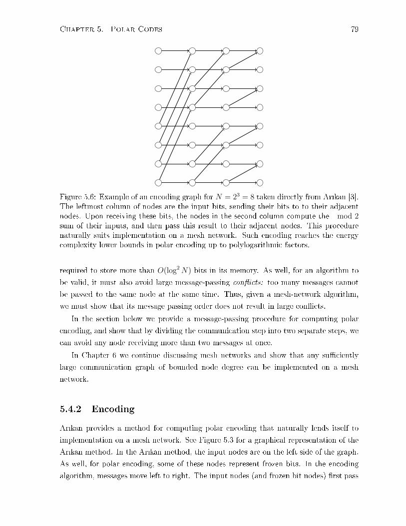
Chapter 5. Polar Codes 79
Figure 5.6: Example of an encoding graph for N = 23 = 8 taken directly from Arkan [3].The leftmost column of nodes are the input bits, sending their bits to to their adjacentnodes. Upon receiving these bits, the nodes in the second column compute the mod 2sum of their inputs, and then pass this result to their adjacent nodes. This procedurenaturally suits implementation on a mesh network. Such encoding reaches the energycomplexity lower bounds in polar encoding up to polylogarithmic factors.
required to store more than O(log2N) bits in its memory. As well, for an algorithm to
be valid, it must also avoid large message-passing conicts: too many messages cannot
be passed to the same node at the same time. Thus, given a mesh-network algorithm,
we must show that its message passing order does not result in large conicts.
In the section below we provide a message-passing procedure for computing polar
encoding, and show that by dividing the communication step into two separate steps, we
can avoid any node receiving more than two messages at once.
In Chapter 6 we continue discussing mesh networks and show that any suciently
large communication graph of bounded node degree can be implemented on a mesh
network.
5.4.2 Encoding
Arkan provides a method for computing polar encoding that naturally lends itself to
implementation on a mesh network. See Figure 5.3 for a graphical representation of the
Arkan method. In the Arkan method, the input nodes are on the left side of the graph.
As well, for polar encoding, some of these nodes represent frozen bits. In the encoding
algorithm, messages move left to right. The input nodes (and frozen bit nodes) rst pass

Chapter 5. Polar Codes 80
their bits to the node to which they are connected in the adjacent column of nodes. The
nodes in this column proceed to compute the modulo 2 sum of their inputs, and pass
the result to their adjacent nodes on the right. This continues until the nal column is
reached, resulting in the codeword.
In our proposed mesh-network implementation, each of the N processor nodes corre-
sponds to a row of nodes in the encoding graph of Figure 5.6. Obviously, if each message
(which corresponds to an edge in the graph) is to be sent one-by one, such an order of the
message-passing procedure would avoid conicts and would be easily be implementable
on a mesh network. (In fact, this is the way we propose to do decoding). However, much
of the computation for encoding can be done in parallel. We show in Appendix A.8 how
a constant fraction of the messages corresponding to edges connecting nodes in adjacent
columns can be sent simultaneously in a way that avoids conicts.
5.4.3 Analysis of Mesh Network Encoding Algorithm Complex-
ity
Note that there at Θ(log2N) stages of the encoding algorithm (easily seen from Fig-
ure 5.6). Suppose the number of clock cycles used by an individual node for reading an
address and computing which direction to send its message is TR. Suppose that the com-
plexity for computing parity of the received bit with the current bit is TP . At each stage,
the number of hops between processor nodes is at most O(√N). There are Θ(logN)
stages. Thus, the number of clock cycles required is
T = Θ(
logN(√
NTR + TP
))
The computation of parity can obviously be done in time Θ(1). The routing requires
computing which direction to send the message: up, right, or left. This can easily be
accomplished in Θ (logN) time (that is, proportional to the length of the address).
The proposed algorithm also uses roughly the same fraction of node each clock cycle,
so we can assume for scaling rules the switching activity factor (q) is constant. The area
of such a circuit scales as A = Θ(log2N). Thus:
E = qAT = Θ(N3/2 log4N)

Chapter 5. Polar Codes 81
5.4.4 Decoding Mesh Network
Clearly, because of the requirement of successively computing each estimate in polar
decoding, asymptotically the number of clock cycles for a polar decoding scheme must
scale at least as Ω(N). A fully parallel polar decoder thus must have area-time complexity
at least Ω(N2).
However, the algorithm proposed by Arkan [3] that takes time complexity O(N logN)
can easily be implemented on a mesh network. Each node of the mesh network corre-
sponds to a row of nodes of the graph in Figure 5.3. As described by Arkan [3], a depth
rst message-passing procedure between the nodes of the graph can compute the polar
decoding in Turing time complexity O(N logN). The distance between any two nodes in
a mesh network is not greater than O(N1/2). Thus, decoding on a mesh network takes
A = Θ(N log2N
)and T = Θ(N3/2 log2N), where the algorithm takes O(N logN) steps,
and O(N1/2 logN) time to do the message passing. Since a fully parallel decoding algo-
rithm requires only a single processing node to be active at a given time, the switching
activity factor of this scheme scales as Θ (1/N). Thus the energy of the computation
scales as E = O(N3/2 log4N
).
5.5 Generalized Polar Coding on a Mesh Network
Arkan [3] proposes a generalization of polar codes in which the generator matrix is no
longer G1 as dened in Section 5.2. Korada et al. [4] analyze such schemes and show that
there exist generating matrices in which for suciently large N , PN ≤ e−Θ(N1−ε) for any
ε > 0. That is, they are e−n1−ε
-coding schemes. By [5, Theorem 1], such circuits must
have bit-meters energy that scales as E ≥ Ω(N3/2−ε/2). Both [3] and [4] argue that such
schemes have O(N logN) time complexity algorithms for decoding. When implemented
on a mesh network, such algorithms would take energy complexity Θ(N3/2 log4N) for
the same reasons described in Section 5.4.4. Thus, we can say that the general lower
bounds can be almost reached for such close-to-exponential coding schemes (that is,
within a factor of N εpolylog(N)). Such a scheme would have a switching activity factor
q that scales as Θ(1/N). Such a circuit would take number of clock cycles that scales
as T = Θ(N3/2 log2N). Note however that Theorem 2 suggests a lower bound T (N)
of Ω(N1/2), and thus this method does not simultaneously reach these energy and time
lower bounds.
Thompson model lower bounds for time and energy of Chapter 3 for f(N)-encoder
energy and time complexity can be reached with polar encoding up to an N εpolylog(N)

Chapter 5. Polar Codes 82
factor for small ε by using an appropriately chosen generator matrix for the construction
of [4]. This is because parallelization of the encoding procedure is possible. For any xed
ε, the communication graphs of such encoders will have constant node degree, so we can
naturally apply the results of Chapter 6 and use the one-hop communication step passing
procedure of this chapter to implement encoding on a mesh network with energy close
to the universal lower bounds.
5.6 Energy Scaling as Function of gap to Capacity
In this section, we consider how the energy of polar codes scales as capacity is approached.
Denition 64. For a particular code, let χ = 11−R
C
be the reciprocal gap to capacity.
Note that as rate approaches capacity, χ approaches innity.
Guruswami et al. [70] show that as a function of reciprocal gap to capacity, the
block length required to achieve a set probability of block error Pe for polar codes scale
as N = O (χµ) for some value µ; that is, the block length scales polynomially in the
reciprocal gap to capacity. A line of research by Hassani et al. [71], Goldin et al. [72]
and Mondelli et al. [73] show that 3.579 ≤ µ ≤ 4.714. These bounds, combined with
Theorems 9 and 10 and the discussion in Section 5.4 that bound energy of encoding and
decoding in terms of N by:
Ω(N1.5
)≤ Ecomp ≤ O
(N1.5 log4N
)
imply an obvious corollary.
Corollary 7. The energy for polar encoders with reciprocal gap to capacity χ and a set
probability of block error, in which C > 12, is bounded by:
Ω(χ5.3685
)≤ Ecomp ≤ O
(χ7.071 log4 (χ)
)(5.12)
with decoding energy bounded similarly.
Note that polar codes are e−N12−ε-codes [74] for any ε > 0. We can apply the well
known general lower bound on block length of any code as a function of fraction of
capacity [60] of N ≥ Ω(χ2) and the general lower bound of [75, Theorem 1] to show that
all e−N12−ε-encoding and decoding schemes have energy bounded by:
E ≥ Ω(N
54−ε)≥ χ2.5
Chapter 5. Polar Codes 83
When contrasted with the lower bounds of (5.12), this illuminates a gap between general
lower bounds and that which is achievable through polar coding.

6Mesh Networks
In this chapter, we expand on the analysis of the mesh network that we showed could be
used to perform polar encoding and decoding in Chapter 5. The polar encoding analysis
involved showing that the message passing steps of polar encoding could be carried out
on a mesh network.
In Section 6.2, we show that a large class of communication graphs of algorithms can
also be implemented on a mesh network with only a logarithmic overhead in number of
clock cycles. This implies in particular that the Ω(N1.5) lower bound for serialized LDPC
decoders of Theorem 7 is tight up to a polylogarithmic factor.
In Section 6.3, we show that, for each valid f(N), conditioned on an assumption re-
garding the iterative decoding performance of LDPC codes, our E ≥ Ω(N√− log(f(N))
energy lower bound of Theorem 1 and number of clock cycles lower bound of T ≥√− log(f(N)) of Theorem 2 for codes that reach the energy lower bound can be reached
up to a polylogarithmic factor. Even if the assumption is not true, the parallel construc-
tion of Section 6.3 can reach the energy lower bounds up to a N ε polylog(N) factor by
using generalized polar codes of [4] that we discussed in Section 5.5.
Placing many decoders in parallel, as we suggest in the construction of Section 6.3 is
a common technique for code design. In the literature, placing polar decoders in parallel
was analyzed in [76] and such circuits had good performance, providing some practical
84

Chapter 6. Mesh Networks 85
justication for the theoretical results of this chapter.
In Section 6.1 we discuss how the mesh network communication step can be broken
into one-hop communication steps. In Section 6.2 we prove the main technical result of
this chapter, namely that with high probability a random orientation does not result in
a high number of conicts. Finally, in Section 6.3 we show how parallelization of polar
codes and LDPC codes can be used to construct close to energy optimal f(N)-decoders.
6.1 Mesh Network
Recall the discussion of the mesh network from Chapter 5, Section 5.4, in which we showed
that polar encoding can be done on a mesh network with no large conicts. We considered
placing the nodes in a raster-scan ordering and showed that by dividing the message-
passing steps into two separate message-passing steps, no single node has to process more
than one message in a single step. In this section, we modify the message-passing step by
dividing it into one-hop communication steps and show that this technique can be used
to implement all suciently large communication graphs of bounded node degree on a
mesh network. To do so, we will use the probabilistic method and consider randomly
placing the vertices of the graph onto the mesh network.
Recall that a computation on a mesh network consists of communication steps and
computation steps. In a communication step, the processor nodes are to send messages
to other processor nodes in parallel. Associated with such a step is a communication
graph. A communication graph is a directed graph, where each vertex corresponds to
a processor node and an edge directed from vertex a to vertex b exists if and only if,
during the communication step, node a sends a message to node b. In such a scenario
we call node a the source of the message and node b the target of the message. In LDPC
decoding, the nodes of the mesh network may correspond to check and variable nodes,
and the communication graph associated with one iteration would be the Tanner graph
of the underlying code.
Denition 65. The orientation of a graph with N nodes on a mesh network of N nodes
is an assignment of the graph nodes to the nodes of the mesh network.
Note that there are N ! possible orientations for a given graph.
We divide the communication step of an algorithm into multiple one-hop commu-
nication steps. Before every such step, we assume that each processor node contains
message-address pairs in their memory that are to be sent to another node in the circuit.
We let κmax be the maximum number of message-address pairs contained in the memory

Chapter 6. Mesh Networks 86
of any processor node during the execution of an algorithm. By dividing the one-hop
communication step into κmax clock cycles, all the messages stored in the memory of each
processor can be communicated from one adjacent node to another during each one-hop
communication step. When κ messages are received by a single processor node in a single
one-hop communication step, such an event is called a κ-conict and κ is the size of the
conict. Note that the size of κmax cannot exceed O(log(N)) because each node is to
hold all the size Θ(log(N)) message-address pairs in its memory at the beginning of each
one-hop communication step, and only has Θ(log2(N)) memory.
The internal circuitry of each processor node can determine to which adjacent node
each of its messages should be sent. A very natural method to implement this we call the
up-down left-right protocol. In this protocol, in determining where to send a message, if
the current node is not in the same row as the target node, the node sends the message-
address pair in the direction (up or down) that gets closer to the target node. If the
node and target are on the same row, then the node sends the message left or right,
whichever is closer to the target. Note that once an orientation is chosen for the nodes
with a particular communication graph, the up-down left-right protocol can be carried
out, so long as there are no conicts bigger than O(log(N)).
Note that a one-hop communication step takes on the order of κmax clock cycles,
and since the Manhattan distance between any two nodes in a mesh network is at most
2√N , we conclude that such a communication step takes number of clock cycles T =
Θ(κmax√N). For a communication protocol to be valid for a mesh-network, it must be
that no computational node is required to store more than O(log2N) bits in its memory,
and thus κmax cannot exceed O(log(N).
In the following section, we show that algorithm with a communication graph of
maximum degree dmax can be implemented with κmax < log(N). The key idea is that for
suciently large graph with bounded maximum node degree, there exists an orientation
of the graph such that the up-down left-right protocol results in no more than Θ(log(N))
message-address pairs to be processed by any single node during any one-hop communi-
cation step. To do so we will use the probabilistic method to show that asymptotically,
almost all orientations have no conicts bigger than log(N) when the up-down left-right
protocol is used.

Chapter 6. Mesh Networks 87
6.2 Communication Protocols with Low κmax Exist For
Most Graphs
We consider a particular node labelled i. There are two types of conicts: same-column
conicts, and dierent-column conicts. Conicts occur at one-hop communication step
τ when a message originating at a node (called the source node) at a Manhattan distance
τ away from node i is received at node i at the τth one-hop communication step. Conicts
that occur at the τ -th one-hop communication step are called τ -distant conicts.
Denition 66. A same-column conict occurs when a source node is above the node of
interest and has an edge connected to a node below the node of interest.
For each τ , there are at most 2dmax τ -distant same-column conicts (because there
are only at most 2 nodes distance τ away from any given node on the same column, each
of which sends at most dmax messages.
Denition 67. A dierent-column conict occurs when nodes that do not share the
same row are connected to a node on the same row as node i.
We divide the dierent-column conicts into two types: those whose message starts
from the right and those whose message starts from the left of node i.
Denition 68. We call those starting on the right the right-origin conicts and those
that start on the left the left-origin conicts.
Consider a particular node i. Let the set of nodes that are τ -distant from node i and
to its right be denoted SR. Let the set of nodes in the same column as node i to its left
be TL. We give an illustration of a circuit with the sets SR and TL labelled in Figure 6.1.
Note that all conicts originating from the right τ -distant slots must have a target in
TL.
Remark 7. Observe that SR forms a half-diamond pattern as in Figure 6.1. Observe then
that the size of SR can be no greater than√N because each node in SR must occupy a
dierent row, and there are only√N rows in a mesh network.
Remark 8. Observe that a row has at most√N nodes in a mesh network. Thus, it is
obvious to see that TL ≤√N for all mesh nodes i.
Denition 69. For a graph G = (V,E) and a given subset of vertices X ⊆ V , we can
dene a minimal κ-connected set which is a set of vertices in V \ X that have exactly
κ edges connected to the vertices in X, and in which each node has at least one edge

Chapter 6. Mesh Networks 88
iTLSR
Ss
Figure 6.1: Image of an N = 49 mesh network with a particular node i labelled. Alsolabelled at the left-target nodes (labelled TL) and the right-source nodes of distance τ = 3away from node i. Observe that for τ = 3 all right-origin conicts must originate in theSR right-source nodes as labelled. The key idea of the proof is that for the up-down left-right protocol to result in right-originating conicts at node i at one-hop communicationstep τ , nodes in SR must be connected to nodes in TL. The nodes labelled Ss are thepossible source nodes of a same-column conict.

Chapter 6. Mesh Networks 89
connected to a vertex in X. For a set X we denote the set of all minimal-κ-connected
sets as Mκ(X)
We will bound the number of orientations that result in size κ right-origin conicts.
The number of orientation that result in κ-left origin conicts is bounded exactly the
same way.
We rst prove some preliminary lemmas.
Lemma 22. The number of right-originating conicts of a graph with maximum node
degree dmax at a particular one-hop communication step at a particular node is at most
dmax
√N .
Proof. We conclude this by observing there are at most√N nodes to the right of any
node in the circuit that are a constant Manhattan-distance away from this node.
Lemma 23. The expression
bi =
(c√N
i
)(√N
i
)i!(N − i− Z)!
decreases with increasing i when i < X, N − i − Z > 0, logN < i < c√N , c > 0 for
suciently large N .
Proof. Observe that:
(√N
i
)(√N
i
)i!(N − i− Z)! =
(c√N)!(√N)!
i!(√N − i)!(
√N − i)!
(N − i− Z)!
and thusbi+1
bi=
(c√N − i)(
√N − i)
(i+ 1)(N − i− Z)
Applying the bound on i that logN < i < c√N we have
bi+1
bi≤ (c√N − logN)(
√N − logN)
(logN + 1)(N − c√N − Z)
Note that the denominator grows as Θ(N logN) while the numerator grows as Θ(N).
Thus, for suciently large N this quantity is less than 1, and so bi decreases with in-
creasing i.
Lemma 24. The quantity
bk =
(N
k
)(k)!(N − c− k)!

Chapter 6. Mesh Networks 90
increases with k when 0 < k < N , c > 0, and N − c−k ≥ 0, and N , c, k are all integers.
Proof. Observe that
bk+1
bk=
N !(N−k−1)!
(k + 1)!(N − c− k − 1)!
N !(N−k)!
(k)!(N − c− k)!
=(k + 1)(N − k)
(N − c− k)
which is greater than 1, because N − k ≥ N − c− k (a consequence of c > 0).
For a given graph of N nodes, and a particular mesh network computational node i,
we let Rκi,τ be the number of orientations of the nodes such that the up-down left-right
protocol results in a size κ right-originating conict at node i at communication step τ .
Similarly, we let Lκi,t be the number of orientations that result in a left-originating conict
at node i at communication step τ .
Lemma 25. Consider a graph with N vertices and maximum node degree dmax ≥ 1 and
place these nodes uniformly randomly on a mesh network of size N . If N is suciently
large, then the probability that this orientation combined with the up-down left-right proto-
col results in a κ right-originating conict at mesh node i at communication step τ ≤ 2√N
is bounded by
P (Rκi,τ ) ≤ exp(−Θ(log logN logN))
when logN ≤ κ ≤ dmax
√N .
Proof. We will count the number of orientations of the nodes that results in at least a size
κ conict originating from the right. To do so we will sum up over all choices of left target
nodes and all minimum-κ-connected sets of these left target nodes (which will form the
source nodes of the messages that conict at node i). Note that if there is a size κ right-
originating conict then there is a set of nodes in SR that are connected to TL by exactly
κ edges. Thus, there must be a set of nodes in SR that form a minimal-κ-connected set
of TL.
Thus, we observe that:
Rκi,τ ≤
∑
X⊆V ||X|=|TL|
∑
Y∈Mκ(X)
|TL|!(|SR||Y |
)|Y |!(N − |Y | − |TL|)! (6.1)
This is the sum over all choices of |TL| nodes to be places in the |TL| target node positionand all and all choices of minimal-κ-connected sets Y for that set X. For each such choice

Chapter 6. Mesh Networks 91
of target nodes and minimal-κ-connected set, the term |TL|! is the number of ways to
permute the |TL| left target nodes,(SR|Y |
)the number of ways to place the |Y | source nodes
in the SR right τ -distant mesh node locations, and |Y |! the number of ways to permute
these nodes. (N − |Y | − |TL|)! is the number of ways to permute the remaining nodes.
We now bound this quantity.
Note that for every subset of X nodes of our graph and Y ∈ Mκ(X) (that is, for all
sets Y that are minimal κ-connected to a set of vertices X) dmax|Y | ≥ κ because there
must be at least κ edges connected to the elements of Y . Thus:
|Y | ≥ κ/dmax (6.2)
Moreover, for all X ⊆ V and Y ⊆Mκ(X),
|Y | ≤ κ (6.3)
because in a minimally κ-connected set at least every node must be connected to a node in
X; if there were more than κ such nodes then the set would be at least (κ+1)-connected.
As well, from Remark 7 the number of right source nodes of distance τ from node i
is bounded by:
|SR| ≤√N. (6.4)
Also, from Remark 8 the number of left targets of these nodes is bounded by:
|TL| <√N (6.5)
Now, consider any particular X ⊆ V . Let Mk,i(X) denote the minimal κ-connected
neighborhoods of X of size i.
For compactness we dene
S1 =∑
Y∈Mκ(X)
(|TL|)!(|SR||Y |
)|Y |!(N − |Y | − |TL|)!
which is the second summation in the expression in (6.1).
We then note that for a particular X ⊆ V where |X| = |TL|,
S1 =κ∑
i= κdmax
|Mk,i(X)|(|TL|)!(|SR|
i
)|i|!(N − i− |TL|)!

Chapter 6. Mesh Networks 92
Note that there are at most dmax
√N possible neighbours of the vertices in X. Thus,
number of the κ-connected sets of a set X of size i is upper bounded by
|Mκ,i(X)| ≤(dmax
√N
i
)
since each element of a κ-connected set must have at least one edge connected to a vertex
in X. So then, applying as well (6.4)
S1 ≤κ∑
i= κdmax
(dmax
√N
i
)(TL)!
(|SR|i
)i!(N − i− |TL|)!
We have that |SR| ≤√N for all τ ≤ 2
√N and so:
S1 ≤κ∑
i= κdmax
(dmax
√N
i
)(TL)!
(√N
i
)i!(N − i− |TL|)!
If logN < κ < dmaxN12 for ε > 0, then the expression to the right of the summation
decreases with increasing i by Lemma 23 . Thus, for suciently large N , the expression
is maximized when i = κdmax
. This allows us to conclude:
S1 ≤κ∑
i= κdmax
(dmax
√N
κdmax
)(|TL|)!
(√Nκ
dmax
)i!(N − κ
dmax
− |TL|)!
≤(κ− κ
dmax
+ 1
)(dmax
√N
κdmax
)(|TL|)!
(√Nκ
dmax
)(κ
dmax
)!(N − κ
dmax
− |TL|)!
Substituting the above bound in (6.1) gives us:
Rκi,tτ ≤
∑
X∈V ||X|=TL
(κ− κ
dmax
+ 1
)(dmax
√N
κdmax
)(|TL|)!
(√Nκ
dmax
)(κ
dmax
)!(N − κ
dmax
−|TL|)!
We then conclude that:
Rκi,τ ≤
(N
|TL|
)(κ− κ
dmax
+ 1
)(dmax
√N
κdmax
)(|TL|)!
(√Nκ
dmax
)(κ
dmax
)!(N − κ
dmax
− |TL|)!.
Note that the size of TL depends on the location of node i. Lemma 24 shows this
expression increases with TL. Combining this with the observation that TL ≤√N for all

Chapter 6. Mesh Networks 93
nodes i, we can show that:
Rκi,tτ ≤
(κ− κ
dmax
+ 1
)(N√N
)(√N)!
(dmax
√N
κdmax
)(√Nκ
dmax
)(κ
dmax
)!(N − κ
dmax
−√N)!.
This is an upper bound on the number of permutations of the nodes of a graph that
will results in a right originating κ-conict at communication step τ . Since there are N !
permutations, the probability of this event is given by:
P(Rκi,tτ
)≤
(κ− κ
dmax+ 1) (
N√N
)(√N)!(dmax
√N
κdmax
)( √Nκ
dmax
) (κ
dmax
)!(N − κ
dmax−√N)!
N !
≤
(κ− κ
dmax+ 1)N√N(dmax
√N
κdmax
)( √Nκ
dmax
) (κ
dmax
)!
(N − κ
dmax−√N) κdmax
+√N
≤
(κ− κ
dmax+ 1)N√N(dmax
√N
κdmax
)( √Nκ
dmax
) (κ
dmax
)!
(N − κ
dmax−√N)√N (
N − κdmax−√N) κdmax
Using(nk
)≤ nk
k!on the
(dmax
√N
κdmax
)(3√Nκ
dmax
)terms and simplifying, we get:
P(Rκi,τ
)≤
(κ− κ
dmax+ 1)N√N(dmax
√N) κdmax
(√N) κdmax
(N − κ
dmax−√N)√N (
N − κdmax−√N) κdmax
(κ
dmax
)!
Continuing to simplify this expression we get:
P(Rκi,τ
)≤ N
√N
(N − κ
dmax−√N)√N
Nκ
dmax
(N − κ
dmax−√N) κdmax
(dmax)κ
dmax
(κ− κ
dmax+ 1)
(κ
dmax
)!
.
As N approaches innity, the rst two quotients in the above product approach 1, so in
particular for suciently large N :
N√N
(N − κ
dmax−√N)√N
Nκ
dmax
(N − κ
dmax−√N) κdmax
≤ 1 + ε

Chapter 6. Mesh Networks 94
for any ε > 0 and thus, for suciently large N :
P(Rκi,τ
)≤
(1 + ε) (dmax)κ
dmax
(κ− κ
dmax+ 1)
(κ
dmax
)!
From Stirling's approximation we know that:
N ! ≥(N
e
)N
and so:
P(Rκi,τ
)≤
(dmax)κ
dmax
(κ− κ
dmax+ 1)
(κ
edmax
) κdmax
Observe that this decreases with increasing κ. Thus if κ > log(N) this implies:
P(Rκi,τ
)≤ exp(−Θ(log logN logN)).
Note that this is less than cN−k for any k > 0 and suciently large N .
Let R∗κ be the event that a random orientation of the nodes has a right-originating
conict of size κ or greater.
Corollary 8. The probability that there is a conict of size logN or greater from nodes
originating from the right at any one-hop communication step and at any node is bounded
by:
P(C∗logN
)≤ exp(−Θ(log logN logN))
Proof. Observe that
R∗logN =N⋃
i=1
√N⋃
j=logN
2√N⋃
τ=1
Rτi,j
that is, the set of permutations of nodes resulting in right-originating conicts of size
dmax logN or greater is the union of all the events Rτi,j, where we recall Rτ
i,j is the set
of permutations that results in a right originating conicts of size j at node i during

Chapter 6. Mesh Networks 95
computation step t. Thus:
P(R∗logN
)≤
N∑
i=1
√N∑
j=logN
2√N∑
t=1
exp(−Θ(log logN logN))
≤ 2N2 exp(−Θ(log logN logN))
≤ exp(−Θ(log logN logN)). (6.6)
Lemma 26. Consider a sequence of communication graphs with maximum node degree
dmax and increasing number of vertices N . If the nodes of a such a graph are uniformly
randomly placed on a mesh network, then the probability that for this orientation the up-
down left-right protocol results in a κ-conict where κ > 2dmax logN + 2dmax approaches
0 with increasing N .
Proof. Note that by a symmetrical argument the probability of collision originating from
left nodes of size greater than logN (denoted by event L∗logN) is bounded by:
P(L∗logN
)≤ exp (−Θ(log logN logN)) (6.7)
We let the event that the random orientation results in a conict of size 2 logN+2dmax or
greater as X∗2 logN+2dmax. Note that, if a permutation has a collision of size 2 logN+2dmax,
then, necessarily either there exists a right-originating collision of size logN or greater
or a left-originating collision of size logN or greater (Otherwise their sum cannot exceed
2 logN + 2dmax since at most 2dmax collisions at a particular location are same-column
conicts).
Thus:
X∗2 logN+2dmax⊆ R∗logN ∪ L∗logN
Applying (6.6 and ), (6.7 ) and union bounds gives us:
P(X∗2 logN+2dmax
)≤ 2 exp(−Θ(log logN logN))
which approaches 0 with increasing N .
Corollary 9. All sequences of communication graphs with bounded maximum node degree
can be implemented on a mesh network with A = Θ(N log2N), and T = N1/2 log2(N).
Proof. First, since the probability that a random permutation has a 2 logN + 2dmax
conict approaches 0, then, for large enough N , there just exists at least one orientation

Chapter 6. Mesh Networks 96
of the nodes of the graph on a mesh network with a conict less than 2 logN+2dmax when
the up-down left-right protocol is used. Consider this orientation, and then divide each
one-hop communication step into at most 2 logN + 2dmax = Θ(logN) clock cycles. The
number of one-hop communication steps needed is at most 2√N . When implementing
the up-down left-right protocol, at most O(log(N)) clock cycles are needed to process
each address. Combining these observations leads to the bound on T in the corollary
statement. The bound on A is simply the area of the mesh network.
An obvious corollary of Corollary 9 is that all sequences of LDPC codes with bounded
node degree can be implemented on a mesh network with energy that scales as A =
Θ(N log2N), and T = niterN1/2 log2(N) where niter is the number of iterations. This
reaches the lower bound scaling rule for serialized LDPC decoders of Theorem 7 for
sequences of LDPC codes of constant maximum node degree.
6.2.1 LDPC Codes on a Mesh Network
Remark 9. (On notation) In what follows, we let polylog(N) denote a function that grows
no faster than logα(N) for some α > 0; that is, this represents a function that grows at
most polylogarithmically in N .
In this section we will show how to construct an f(N)-coding scheme that reaches
the information-friction energy bound of [5] up to an N ε polylog(N) factor for any ε > 0.
The construction can also reach our energy lower bounds of Theorem 1 and number of
clock cycles lower bound of Theorem 2 up to polylogarithmic factors, conditioned on an
assumption. The assumption we make is as follows:
Assumption 1. There exists a sequence of LDPC codes and decoders for the BEC
with bounded maximum Tanner graph node degree, number of iterations that scales as
polylog(N), and probability of error that scales as e−Θ(N).
One approach that exists in the literature to analyze iterative LDPC code performance
involves analyzing the probability of stopping sets. With the assumption of innite
number of iterations, Burshtein et al. [77] show that there exist LDPC codes with error
probability that scales as e−cN , consistent with part of our assumption. However, this
encounters a problem because the stopping set approach must assume an innite number
of iterations. Of course, since when decoding for the BEC each iteration must correct at
least one error (or else a stopping set has been encountered) there can be at most O(N)
iterations. However, this is more than polylogarithmically in N and thus this does not
prove our assumption.

Chapter 6. Mesh Networks 97
Another method used to analyze error probability performance in terms of number of
iterations is by Lentmaier et al. [78]. This method involves showing that a random Tanner
graph is, with high probability, locally tree-like, allowing for independent iterations, and
thus bit error probability can be analyzed recursively. The problem with this method is
that after the graph is no longer locally tree-like, the independent iteration assumption
breaks down. The authors show that if Θ(log(N)) iterations are carried out for some
regular LDPC codes, then bit error probability is bounded as e−Θ(Nα) for some 0 < α ≤ 1,
but it is not proven that α = 1 is achievable.
However, if Assumption 1 is true, we can use such codes to construct f(N)-decoding
schemes that are energy and time optimal (within the Thompson model) up to polylog-
arithmic factors for any f(N) ≤ e−Θ(N). Even if the assumption is not true, generalized
polar decoders can also be used to construct close to energy optimal decoders for each
f(N) ≤ e−Θ(N1−ε) for any ε > 0. We show how to construct such decoders in the next
section.
6.3 Using Parallelization to Construct Close to Energy
Optimal f (N)-coding Schemes
The following analysis works for both encoders or decoders in parallel. Without loss of
generality, we assume we are constructing decoders.
We begin by assuming we can construct an e−cN -decoding scheme with energy that
scales as E(N) ≤ O(N1.5 polylogN), for some c > 0. If Assumption 1 is true, then this
can be an LDPC decoder implemented on a mesh network. If not, then this can be a
generalized polar decoder as discussed in Section 5.5, requiring only a slight modication
of the derivation below (which we discuss in Section 6.3.1.
Consider placing N/M of such circuits in parallel, where each circuit has block length
M , thus creating a circuit with total block length N .
The energy of such a parallel scheme is simply the sum over all the individual energy
consumptions of each of the individual subcircuits in parallel. Thus:
E ≥ c′NM12 polylog(M)
for some c′ > 0. An error occurs if any of the decoders make an error, and so by union
bound:
Pe ≤N
Me−cM

Chapter 6. Mesh Networks 98
Consider a function f(N) that approaches 0 with increasing N and f(N) ≤ e−cN for
some c > 0 and suciently large N . To construct an f(N)-coding scheme, we simply
then choose M to scale with N appropriately. So, we let
M = −1
clog
(f(N)
N
)(6.8)
implying that the parallel circuit will have probability of error bounded as
Pe ≤1
−1c
log (f(N)/N)f(N) ≤ f(N)
and thus we have an f(N)-coding scheme.
The energy of such a scheme scales as:
E ≤ N
√−1
clog
(f(N)
N
)polylog
(−1
clog
(f(N)
N
))
Noting that − log(f(N))/N < N for suciently large N by our assumption on f(N) and
simplifying:
E ≤ N
√1
c
√− log(f(N)) + log(N) polylog(N)
Using√x+ y ≤ √x+
√y and letting c′′ =
√1c:
E ≤ c′′N[√− log(f(N)) +
√log(N)
]polylog(N) = Θ(N
√− log(f(N)) polylog(N)
This construction is thus a polylogarithmic factor away from the universal information
friction lower bounds implied by Grover [5].
6.3.1 Analyzing Area and Number of Clock Cycles
We can also analyze this parallel construction in terms of how T and A scale with N . If
the decoders placed in parallel are LDPC codes consistent with Assumption 1, then:
T ≤M0.5 polylog(M)
and so as a function of block length N
T ≤√− log(f(N)) polylog(N)

Chapter 6. Mesh Networks 99
that is, a polylogarithmic factor away from the lower bound on number of clock cycles
for energy optimal decoders of Theorem 2 in Chapter 3.
Of course, the construction of this time and energy optimal f(N)-coding scheme
depends on Assumption 1. Whether this is possible remains an open question.
Nonetheless, we can still easily construct a close to energy optimal f(N)-coding
scheme by using a generalized polar code with error probability that scales as e−cN1−ε
as
discussed in Chapter 5. This reaches the information-friction lower bounds of up to an
N ε polylog(N) factor; however, it does not reach our time lower bounds of Theorem 2.
To show this, we can simply modify our choice of M as a function of N in (6.8) above
by choosing
M = −(
1
clog
(f(N)
N
))( 11−ε)
which will have energy that scales as
E ≤ O(N [− log(f(N))](
12− ε
2) polylog(N)
)
which for all f(N) < e−cN is an N ε polylog(N) factor away from the energy optimal lower
bound.

A poet once said, `The whole universe is in a
glass of wine.' We will probably never know
in what sense he meant it, for poets do not
write to be understood. But it is true that if
we look at a glass of wine closely enough we
see the entire universe... If our small minds,
for some convenience, divide this glass of wine,
this universe, into parts physics, biology, ge-
ology, astronomy, psychology, and so on re-
member that nature does not know it! So let
us put it all back together, not forgetting ulti-
mately what it is for. Let it give us one more
nal pleasure; drink it and forget it all!
Richard Feynman 7Information Friction in
Three-Dimensional Circuits
So far our discussions have been of planar circuits. However, circuits implemented in
three-dimensions exist [79], and so we generalize the recent information friction (or bit-
meters) model introduced by Grover in [5] to circuits implemented in three-dimensions
and extend the technique of Grover to show that, in terms of block length N , a bit-meters
coding scheme in which block error probability is given by Pe(N) has encoding/decoding
energy that scales as Ω(N (− lnPe (N))
13
). We show how this approach can be general-
ized to an arbitrary number of dimensions.
The information friction computational energy model, introduced by Grover in [5],
was further studied by Vyavahare et al. in [80] and Li et al. in [81].
The information-friction model is very similar to the Thompson model. In fact, the
Ω(N√− log(f(N))) lower bound on energy for f(N)-coding schemes derived for fully-
parallel decoders in Chapter 3 is also implied by Theorem 1 in [5] (although no bounds
on number of clock cycles are derived using this technique like we derive in Chapter 3).
Nonetheless, the Grover result is stronger in one sense: it does not require an assumption
on bounded switching activity factor.
We generalize (and slightly modify) this model to three dimensions and use a similar
100

Chapter 7. Information Friction in Three-Dimensional Circuits 101
approach to Grover to obtain some non-trivial lower bounds on the energy complexity of
three dimensional bit-meters decoder circuits, in terms of block length and probability
of error. We will discuss how this approach can be generalized to models in arbitrary
numbers of dimensions. We present the model below and then prove our main complexity
result.
• A circuit is a grid of computational nodes at locations in the set Z3, where Z is the
set of integers. Some nodes are inputs nodes, some are output nodes, and some are
helper nodes. Note that Grover [5] considers this model in terms of a parameter
characterizing the distance between the nodes, but since we are concerned with
scaling rules, we will assume that they are placed at integer locations, allowing us
to avoid unnecessary notation. The Grover paper considered scaling rules in which
nodes are placed on a plane, in which the number of dimensions d = 2. In our
results we will discuss the case of d = 3 and afterwards discuss how the approach
can be generalized to an arbitrary number of spatial dimensions.
• A circuit is to compute a function of N binary inputs and K binary outputs.
• At the beginning of a computation, the N inputs to the computation are injected
into the input nodes. At the end of the computation the K outputs should appear
at an output node. A node can be both input and output.
• A node can communicate messages along its links to any other node, and can receive
bits communicated to them from any other node.
• Each node has constant memory, and can compute any computable function of
all the inputs it has received throughout the computation that is stored in their
memory, to produce a message that it can send to any other node.
• We associate a computation with a directed multi-graph, that is, a set of edges
linking the nodes. For every computation, there is one edge per bit communicated
along a link in the computation's associated multi-graph. The cost of an edge in
such a multi-graph is the Euclidean distance between the two nodes that it connects.
Note that if a node communicates m bits to another node in a computation, then
that computation's associated multi-graph must have m edges connecting the two
nodes. This multi-graph is called a computation's communication multi-graph.
• The energy, or the bit-meters, denoted β of a computation is the sum of the costs
of all the edges in the computation's associated multi-graph (that is, the sum of
the Euclidean distances of all the edges).

Chapter 7. Information Friction in Three-Dimensional Circuits 102
λL
λL λL
λL
λL
λL
LL
L
Figure 7.1: A diagram of one nested cube in an (L, λ)-nested cube grid, with the edgelengths labeled. A nested cube grid is an innite grid of such nested cubes. The outercubes each have side length L and the inner cubes each have side length L(1− 2λ) at adistance Lλ from the faces of the outer cube.
We consider a grid of three-dimensional cubes, with inner cubes nested within them.
This object is a generalization of the stencil object dened by [5].
Denition 70. An (L, λ)−nested cube grid is an innite grid of cubes, with side length
L and inner cube side length L (1− 2λ). Note that the inner cubes are centered within
the outer cubes. Fig. 7.1 shows a diagram of one cube in a (L, λ)−nested cube grid, to
which the reader can refer to visualize this nested cube structure. A set of nested cube
grid parameters is valid if L > 0 and 0 < λ < 12.
Note that a nested cube grid can be placed conceptually on top of a bit meters circuit.
We will consider placing a nested cube grid in parallel with the Cartesian 3-space that
denes our circuit. We can specify the position of a nested cube grid that is parallel to
a set of Cartesian coordinates by calling one of the corners of an outer cube the origin,
and then specify the location of its origin. A particular set of parameters for a nested
cube grid and a location for its origin (called its orientation) induces a set of subcircuits,
dened below.
Denition 71. A subcircuit, associated with a particular orientation of a nested cube
grid, is the part of a bit-meters circuit within a particular outer cube.
Nodes in any subcircuit can thus be considered to be either inside an inner cube or
outside an inner cube. For any circuit with nite number of nodes there will thus be
some cubes that contain computational nodes, and some that do not. We can label the
subcircuits that contain nodes with the index i. The number of input nodes in cube i we

Chapter 7. Information Friction in Three-Dimensional Circuits 103
denote ni. The number of output nodes in subcircuit i we denote ki. Furthermore, we
denote the number of input nodes within the inner cube of subcircuit i as kin,i.
Denition 72. We dene kin =∑kin,i, which is the the number of output nodes within
inner cubes, which we will often simply refer to with the symbol kin.
We will show in Lemma 28 that there exists a nested cube grid orientation in which
kin is high.
Denition 73. The internal bit meters of a subcircuit i is the length of all the commu-
nication multigraph edges completely within subcircuit i, plus the length of the parts of
the edges within subcircuit i. This quantity is denoted with the symbol βi. Note that
β =∑
all subcircuits j βj (where we may have to sum over some subcircuits that do not
contain any nodes).
Since a computation has associated with it its communication multi-graph, for a given
subcircuit we can consider the subgraph formed by all the paths that start outside of the
cube and end inside the inner cube. We can group all the vertices of this graph that start
outside the outer cube and call this the source, and group all vertices inside an inner
cube and call it the sink. For this graph we can consider its min-cut, the minimum set
of edges that, once removed, disconnects the source from the sink.
Denition 74. The number of bits communicated from outside a cube to within an inner
cube, or, bits communicated, is the size of this minimum cut. For a particular subcircuit
i we refer to this quantity with the symbol bi.
Remark 10. This quantity is analogous (but not the same) as the quantity bi for the
Thompson circuit model from Denition 6, and thus we use the same symbol. The reader
should not confuse these symbols; the Thompson model denition applies to discussions
in Chapter 3, and the bit-meters model denition applies to this chapter.
If the ni internal bits of a subcircuit are xed, then the subcircuit inside an inner cube
will compute a function of the messages passed from outside the outer cube. Clearly, the
size of the set of possible messages injected into this internal cube is 2bi (since bi is the
min cut of the paths leading from outside to inside.)
Lemma 27. All subcircuits with bits communicated bi have internal bit meters at least
biλL.
Proof. This result ows from Menger's Theorem [82, 83], which states that any network
with min-cut bi has at least bi disjoint paths from source to sink. Each of these paths
must have length at least λL from the triangle inequality.

Chapter 7. Information Friction in Three-Dimensional Circuits 104
Remark 11. This lemma makes rigorous the idea that to communicate bi bits from outside
a subcircuit to within its inner square, the bit-meters this takes is proportional to the
distance from outside an outer square to within an inner square (λL) and the number of
bits communicated.
In the lemma below we show that there exists an orientation of any nested cube grid
such that kin is high.
Lemma 28. For all three dimensional bit-meters circuits with K output nodes, all valid
nested cube grid parameters L and λ, there exists an orientation of an (L, λ)-nested cube
grid in which the number output nodes within inner cubes (kin) is bounded by:
kin ≥ (1− 2λ)3K
Remark 12. Note that the relative volume of the inner cubes is (1− 2λ)3 . This lemma
says there exists an orientation of any nested cube grid in which the fraction of output
nodes within inner cubes is at least this fraction, so this result is not surprising.
Proof. This is a natural generalization of the Grover result (See Lemma 2 of [5]), which
uses the probabilistic method. We consider placing the origin of an (L, λ)-nested cube
grid uniformly randomly within a cube of side length L centered at the origin in the
Cartesian 3-space. We index the K output nodes by i. Let 1in,i be the indicator random
variable that is equal to 1 if output node i is within an inner cube. Then, given the
uniform measure on the position of the cube, the quantity kin is a random variable. We
observe:
kin =K∑
i=1
1in,i, thus
E (kin) = E
(K∑
i=1
1in,i
)
=K∑
i=1
E (1in,i)
=K∑
i=1
(1− 2λ)3 (7.1)
= K (1− 2λ)3
where in (7.1) we use the observation that, for each output node, the probability that it
is in an inner square is proportional to the relative area of the inner square. Thus, the

Chapter 7. Information Friction in Three-Dimensional Circuits 105
expected value of kin is K (1− 2λ)3 and so there must be at least one nested cube grid
orientation in which kin is greater than or equal to that value.
Lemma 29. For all valid nested cube parameters L and λ, ni ≤ (L+ 1)3 and thus for
suciently large L ni ≤ 2L3.
Proof. Intuitively, there cannot be more than on the order of L3 inner nodes in a cube of
volume L3. The (L+ 1)3 bound comes from considering the corner case of a cube whose
sides exactly touch output nodes.
We can now state the main results of this section.
Theorem 11. All 3D-bit-meters decoders for a binary erasure channel with erasure prob-
ability ε of suciently large block length with block error probability Pe have bit-meters β
bounded by:
β >27
512
(ln (4Pe)
2 ln(ε)
) 13
K.
Proof. We consider the number of bits communicated from outside a subcircuit i to
within the inner cube of subcircuit i (bi). It must at least be kin,i to overcome the case
that all the input nodes in the entire cube are erased. If this does not happen, then one
of the output nodes must guess at least one bit, making an error with probability at least12, formally justied by Lemma 1. This allows us to argue that:
Pe ≥ P (error|all ni output bits are erased)
P (all ni output bits are erased)
≥ 1
2εni . (7.2)
If β < λLkin then there exists a subcircuit indexed by i in which bi < kin,i. Suppose
otherwise, i.e. that bi ≥ kin,i for all i, then:
β ≥∑
all subcircuits i
λLbi = λL∑
bi ≥ λL∑
kin,i = λLkin
where we apply Lemma 27 after the rst inequality, and for convenience suppress the
subscript on the summation sign after the rst instance. This contradicts our assumption
that β < λLkin.

Chapter 7. Information Friction in Three-Dimensional Circuits 106
We choose the parameter L in terms of probability of error in order to derive a
contradiction if a circuit does not have high enough bit-meters. Specically, we choose
L =
(ln (4Pe)
2 ln(ε)
) 13
. (7.3)
Consider the nested cube structure that has kin ≥ (1− 2λ)3K that must exist by
Lemma 28. If β ≤ λLkin then there must exist a subcircuit i that has less than kin,i bits
injected into it from outside the subcircuit to within its inner cube. Thus:
if β ≤ λLkin then Pe
(a)
≥ 1
2εni
(b)
≥ 1
2ε2L
3(c)
≥ 2Pe
where (a) ows from (7.2), (b) from Lemma 29, and (c) from the evaluation of this
expression by substituting (7.3). This is a contradiction. Thus, all bit meters decoders
must have
β > λLkin
β > λ (1− 2λ)3 LK
≥ λ (1− 2λ)3
(ln (4Pe)
2 ln(ε)
) 13
K.
The second inequality ows from the fact that we are considering the nested cube struc-
ture in which kin ≥ (1− 2λ)3K that must exist by Lemma 28. We may choose any valid
λ to maximize this bound, and letting λ = 18gives us:
β >27
512
(ln (4Pe)
2 ln(ε)
) 13
K.
Remark 13. Note that this argument naturally generalizes to d-dimensional space, in
which all d-dimensional bit-meters decoders have energy that scales as β ≥ Ω(
(ln (Pe))1d K).
The key step in the proof to be altered is in a modication of Lemma 29 and a choice of
L = c(
ln(4Pe)ln(ε)
) 1din line 7.3 of the proof for some constant c that may vary depending on
the dimension. This implies, among other things, that exponentially low probability of
error decoding schemes implemented in d-dimensions have bit-meters energy that scales
as Ω(N1+ 1
d
). Obviously, the most engineering-relevant number of dimensions d for this
type of analysis are d = 2 and d = 3.

If you take just one piece of information from this blog: Quantum
computers would not solve hard search problems instantaneously
by simply trying all the possible solutions at once.
Scott Aaronson
8Is the Information Friction Model a Law of
Nature?
In the previous chapter, we derived some universal lower bounds for the energy complex-
ity of three-dimensional circuits using a natural generalization of Grover's information-
friction model [5]. Can the linear-in-distance assumption be beaten using clever engineer-
ing? Is the information-friction model inaccurate for some other reason? In this Chapter
we discuss this question. If the assumptions of the model cannot be overcome in our
Universe, then our information friction lower bounds are not merely engineering claims:
they are fundamental energy scaling rules for reliable communication in our Universe.
The main assumptions of the three-dimensional information-friction model of Chap-
ter 7 are (1) each input of a computation is injected into a computational node in three-
dimensional Euclidean space, each of which takes up some volume, and (2) the energy
cost of communicating information in this space is linear in distance. The conjecture that
these assumptions capture fundamental practical engineering limitations in our universe
we call the information-friction hypothesis. Below we discuss a few techniques that may
seem to overcome these assumptions, and we also point out how these techniques, upon
closer inspection, fail for some practical reason.
107

Chapter 8. Is the Information Friction Model a Law of Nature? 108
8.0.2 The Spaceship Channel
In [84], the authors argue that communicating long distances using inscribed matter
is more energy ecient for large distances than communicating using electromagnetic
radiation. The idea is to accelerate the matter (in a spaceship perhaps) pointed in some
direction, letting the message hurtle through space. Examining Equation (1) of [84], it
seems to suggest this can be done with an energy that does not change with distance.
However, absent from the analysis is a discussion of friction in interstellar space. Though
friction is very small in space, it is not 0 because space is not a perfect vacuum (see [85]
and the resources referenced, which show that the density of particles in outer space is
somewhere between 0.06−1000 atoms per cm2). Thus, in the limit of very large distances,
the amount of energy needed would still be roughly proportional to distance (or else the
spaceship would be eventually slowed down by friction before reaching its destination).
Thus, the space-ship channel does not seem to be able to overcome assumption 2 of
the information-friction hypothesis.
8.0.3 The Vacuum Tube Channel (AKA the Hyper-loop Chan-
nel)
Another natural objection to the information friction hypothesis is that, why can't
we create a vacuum tube to remove all friction, in a way similar to the Hyper-loop
promoted by Elon Musk (this proposal has been widely covered in the media, see, for
example, [86]). The obvious objection to this technique is that, even if you could suck
out most of the air from the vacuum tube, engineering limitations would prevent you
from sucking out all of the air. And if the tube is anything but a perfect vacuum, the
energy cost of sending a bit would still be at least proportional to the distance the bit
travelled.
But is this merely an engineering limitation? Is it feasible to suck more and more
air out of longer and longer tubes, so that even though there is some air in them, the
state of the tubes gets arbitrarily closer to being a vacuum? Could this technique be
used to violate the information-friction hypothesis? Or is it fundamentally impossible to
create a perfect vacuum? Modern quantum eld theory suggests, however, that even in
a vacuum state virtual particles spontaneously spring into existence [87]. This suggests
that maintaining a vacuum may be impossible in our Universe, although whether virtual
particles cause friction in communicating information is beyond the scope of this thesis, so
we cannot conclude that this technique would be impossible to overcome the information
friction assumption.
Chapter 8. Is the Information Friction Model a Law of Nature? 109
8.0.4 Electromagnetic Radiation
Using electromagnetic radiation is a widely used communication technique. However, it
is subject to a 1R2 energy density loss as a function of distance R. However, this may be
avoided by capturing the radiation with larger and larger receiving antennas as distance
increases. Though terribly impractical at large distances, at rst glance this may seem to
overcome the linear-in-distance energy cost of communication. However, the fact that a
perfect vacuum may be impossible to obtain, attenuation that is exponential in distance
may cause this technique to fail as well, regardless of how big the receiving antennas are.
8.0.5 Quantum Entanglement
Our results model physical limits of classical computers, but of course we live in fun-
damentally quantum world, and so one may conjecture that using phenomenon like en-
tanglement may be used to communicate information over arbitrary distances with little
energy. However, as Eberhart et al. show [88], communicating information by observing
one part of an entangled quantum system cannot be used to communicate information
to receivers observing another part.
However, quantum mechanics suggests it is possible to communicate more information
than is intuitively obvious using super-dense coding [89]. The idea of super-dense coding
is to rst have Alice and bob share one of two entangled qubits. Alice applies appropriate
unitary operations to her bit which evolves the qubit pair into one of four orthogonal
states. She then sends this bit to Bob, who then observe the qubit pair. Alice sends only
one qubit but Bob in eect receives two bits of information because the qubit pair is in one
of four orthogonal states (which, with an appropriate measurement can be determined
exactly). As surprising as this result is, it does not contradict the information friction
hypothesis, because on qubit still needs to be sent over the channel, so there is a factor
of 2 energy savings at most.
8.0.6 Adiabatic Computing
An area of active research is called adiabatic computing (see [90] for a review). Instead
of charging and discharging the wires each clock cycle, the energy is re-used by the
circuit. Because power dissipation to charge a resistor is proportional to I2R where
I is current and R is resistance (that is, non linearly in I) if current is slowed down
then the power consumption can be made arbitrarily small. If run arbitrarily slowly
then theoretically these devices can consume an arbitrarily small amount of energy per

Chapter 8. Is the Information Friction Model a Law of Nature? 110
operation. The problem with this is that if such a scheme was scaled with N , to overcome
energy scaling losses the circuit would have to be run increasingly slowly to the point of
being impractical.
8.0.7 Superconducting Channel
Superconductors are materials that have zero electrical resistance. So a computer made
out of superconducting material would avoid resistive energy consumption. As well, if
wires in a circuit were replaced entirely by superconductors, there would still be energy
consumption due to charging and discharging the capacitance of the wires (which is a
property of the superconductor's geometry, and not the material that it is made from).
However, I cannot rule out the possibility of adiabatic computations using supercon-
ducting material to avoid energy consumption that scales proportionally with distance.
However, any imperfections in the superconductor would result in some power dissipa-
tion caused by resistance, and this eect would still scale linearly in distance (but the
proportionality constant may be much less than in regular conducting wires).
8.0.8 The Wormhole Circuit
One assumption central to the bit-meters model is that computational nodes are packed
within a Euclidean topology. However, Einstein's general theory of relativity predicts that
space-time can bend in the presence of massive objects. Thus in reality, the Universe
is not actually a Euclidean space. In fact, the existence of Einstein-Rosen bridges (or
wormholes) that connect to otherwise distant points in space are consistent with general
relativity [91]. If it were possible to construct a wormhole, not only would it be possible
to communicate information quickly across such a wormhole, it may also be that the
distance that the information travels would be less, and thus not subject to frictional
eects as we assume in our Theorems.
So does the hypothetical Einstein-Rosen Bridge computer violate the information
friction hypothesis? If we could actually construct a wormhole, and the energy to main-
tain that wormhole was sublinear in the distance between the points that the wormhole
connects, then it seems like yes, general relativity seems to contradict the Euclidean-
space assumption of the information-friction model. However, as far as I am aware no
one knows how to actually construct such a wormhole. Though constructing a circuit
lled with wormholes may be utterly impractical, for this reason I am hesitant to claim
that the hypothesis is a law of nature, rather than just a pretty universal engineering
principle.

The important thing is not to stop questioning; curiosity has its
own reason for existing. One cannot help but be in awe when
contemplating the mysteries of eternity, of life, of the marvelous
structure of reality. It is enough if one tries merely to comprehend
a little of the mystery every day. The important thing is not to
stop questioning; never lose a holy curiosity.
Albert Einstein
9Conclusion
The main idea of the thesis is this: we can classify error control coding schemes in
terms of how their block error probability scales. We have universal lower bounds on
the energy and time complexity of such circuits. We analyze LDPC and polar codes and
show close-to-tight upper and lower bounds on a large class of LDPC and polar encoding
and decoding circuits. By analyzing the mesh network and placing mesh network LDPC
decoders in parallel, conditioned on an assumption, we can reach the universal decoding
lower bounds that use a minimum number of clock cycles. On the other hand, generalized
polar decoding can, without requiring any unproven assumptions, reach universal lower
bounds on energy. However, asymptotically they take signicantly more clock cycles. In
Table 9.1 we summarize the main scaling rule results of this thesis.
There are still some unanswered questions related to the computational complexity of
LDPC decoding, and error control coding in general. We discuss some of these problems
below.
• Theoretically constructing serialized encoding and decoding schemes that are close
to the lower bounds is an area of future work.
• Finding upper bounds for three-dimensional circuits is also an open question,
though I suspect a natural generalization of the mesh-network technique to three
111

Chapter 9. Conclusion 112
Type of CircuitLower Bound on
EnergyTechnique to construct
Achievable upper boundon Energy
Number of ClockCycles with this
scheme
Fully-parallelf(N)-Decoder
Ω(N√− log(f(N))
) Parallel generalizedpolar codes,Section 6.3
O(N1+ε
√− log(f(N)))
),
for ε > 0O (− log (f(N)))
Conditioned onassumption, parallelLDPC codes on meshnetwork, Section 6.3
O(N√− log(f(N)))
)O(√− log (f(N))
)
Fully parallelf(N)-Encoder
Ω(N√− log(f(N))
) Parallel generalizedpolar codes,Section 6.3.1
O(N1+ε
√− log(f(N)))
),
for any ε > 0O(√− log(f(N)))
Constant outputnode serial f(N)-encoder/decoder
Ω (−N log(f(N)) ? ? ?
Increasing outputnode serial f(N)-encoder/decoder
Ω(N (− log(f(N))
1/5)
? ? ?
Directlyimplemented LDPC
decoder
Almost surely Ω(N2)per iteration
Directly-implementedtechnique of Section
4.7O(N2) per iteration O(1) per iteration
Serialized LDPCdecoder
Almost surelyΩ(N1.5) per iteration
LDPC decoding onmesh network,Section 6.2.1
O(N1.5)O(√N) per
iteration
Polar Encoder withR > 1/2
Ω(N1.5)Mesh network,Section 5.4.2
O(N1.5) O(√N)
Polar decoder withR > 2/3
Ω(N1.5)Mesh network,Section 5.4.4
O(N1.5) O(N)
3-D Bit-metersEncoder/Decoderwith Pe ≤ f(N)
Ω(N(− log(f(N)))1/3
)? ? ?
Table 9.1: Table summarizing some of the main scaling rule results in this thesis. Therst column shows the class of circuits considered. The second column shows the lowerbound derived for this class of circuits. The third column gives the technique we an-alyze to get close to these lower bounds. The fourth column shows the energy scalingrules for this technique, and the nal column shows how the number of clock cyclesscales for this technique. We use the notation that a function is in O(f(N)) if it is inO(f(N) polylog(N)). A question mark indicates that this remains an area of future work.

Chapter 9. Conclusion 113
dimensions would likely be eective.
• Proving, (or disproving) Assumption 1 would strengthen, or, respectively, weaken
the results of this thesis.
• Constructing or simulating the mesh network circuits that theoretically have good
asymptotic result is an obvious area of further research. When circuits for a par-
ticular problem size are constructed, I suspect there would require many more
energy minimization techniques employed to make mesh network implementations
comparable to state-of-the art circuits, but this is an open question.
• We've analyzed LDPC and polar codes in this thesis. A theoretical energy analysis
for almost any other type of error control code also remains generally unexplored.
Spatially coupled codes [92] may be particularly suitable for this type of analysis.
• Our asymptotically close to optimal construction of Chapter 6 for f(N)-coding
schemes itself may not be a very useful construction (in particular, putting many
identical decoders in parallel can't possibly decrease the energy per bit costs of
decoding). However, communicating a small amount of information between ad-
jacent parallel decoders may come at only a small energy cost but could possibly
increase code performance. Consider, for example, the staircase codes of [93]. Such
codes have an iterative decoding algorithm whose communication graph for each
iteration may require only a small amount of communication across the circuit.
Constructing energy ecient, high performance staircase codes circuits thus may
be possible, and remains an area of future work.
• For LDPC codes, the almost sure" scaling rule for the energy of VLSI LDPC
decoders does not exclude the possibility that there are good LDPC codes whose
decoding energy scales more slowly than this (they may simply occur with vanishing
probability). Thus, there may be some good LDPC codes with lower energy"
Tanner graphs that still provide good code performance. Intuition suggests that
for a given channel a code with a lower energy" LDPC decoder may have higher
probability of error. A general analysis of this fundamental tradeo is an open
question.
• In our LDPC coding lower bounds, the dependence on maximum node degree of
our scaling rules is somewhat surprising. In our denitions of LDPC decoders, we
consider a graph that contains the Tanner graph as a minor. It may be that high
degree nodes can be split to decrease the minimum bisection width of a graph and

Chapter 9. Conclusion 114
thus possibly decrease circuit area. A formal analysis of how vertex splitting might
decrease circuit area remains an open question.
• For LDPC codes, it may be that edges of a Tanner graph that connect vertices
that are too far away on the decoder can be modied to connect closer nodes,
with a small cost in error probability. As well, there exist some algorithmic level
modications [94] that may allow energy savings. A theoretical analysis of such
techniques may be informative.
• Extending the polar encoding and decoding lower bounds to all rates is an obvious
area of future work.
• Our decoding lower bounds are for algorithms based on graphs obtained from the
buttery network decoding graph suggested by Arkan [3]. Our lower bound does
not necessarily include all decoders based on successive cancellation decoding for
polar codes. A particular challenge for generalizing this result is in dening precisely
what a circuit that performs a polar decoding algorithm actually is, and thus this
remains an area of future work.
• More generally, for a given application, what technique can be used to choose the
energy-optimal" error control code? Can this analysis improve the energy of real
communication systems? Ganesan et al. [48] discuss this question and show how,
for a reasonable system model, the performance optimal code depends on the circuit
technology used and the nature of the channel.
• All of our results in this thesis are asymptotic. However, real circuits are designed
for a xed problem size. Using energy as a parameter to be traded o with error
probability and rate in the design of real, physical circuits is a little studied problem,
though [48] begins studying this question. In particular, the design of code libraries
with parameters that can be varied that trade o energy and reliability is a natural
extension of this work.
• The decoding problem for communication systems is a special case of the more gen-
eral problem of inference. Well known algorithms used for inference, for example
the Sum-Product Algorithm [95] and variational methods [96], include Gallager's
low-density parity-check decoding algorithms as a special case [43]. Thus, we con-
jecture that there may be similar tradeos between energy, latency, and reliability
in circuits that perform inference. Analyzing the energy complexity of more general
inference problems is thus an obvious area of future work.
AAppendices
A.1 Coding Schemes with Error Probability Less than
1/2
Recall the denition of an r-stage nested bisection, the quantity bi, and the quantity Br,
and Ni Ki from Chapter 3, Section 3.3.
In this section, we will be dividing a circuit up into pieces and then we will let N
grow larger. Technically, a circuit can only be divided into an integer fraction of pieces.
However, this rounding to an integer number of subcircuits does not change our scaling
rules. To make this notion rigorous, we will need to use the following lemma:
Lemma 30. Let h : R→ R be a function such that |h (x)− x| ≤ a for suciently large
x and some positive constant a. If there are functions f, g : R→ R, and g is continuous
for suciently large x, and if limx→∞ f (g (x)) = c for some constant c ∈ R, and if
limx→∞ g (x) =∞ then limx→∞ f (h (g (x))) = c.
Proof. Suppose
limx→∞
f (g (x)) = c.
To show that limx→∞ f (h (g (x))) = c we need to construct, given some ε, a particular
x0 such that for all x > x0, |f (h (g (x)))− c| < ε. Since g grows unbounded, and is
115

Appendix A. Appendices 116
continuous for suciently large x, then there must be a particular value of x (call it x′)
such that g (x) takes on all values greater than g (x′) for some x > x′. As well, for any
ε > 0 there exists some x′′ such that for all x > x′′, |f (g (x))− c| < ε. In particular
this is true for some x′′ > x′. Thus, choose x0 to be the least number greater than x′′
in which g (x0) = g (x′′) + a (this must exist because g takes on all values greater than
g (x′′)). Thus, for x > x0 h (g (x)) only takes on values greater than g (x′′) (because
|h (x)− x| ≤ a). Since |f (g (x))− c| < ε for all x > x′′, thus |f (h (g (x)))− c| < ε for all
x > x0, since h (g (x)) can only take on values that g (x) takes on for x > x′′.
Corollary 10. This result applies when h (·) is the oor function, denotedb·c, since
|bxc − x| ≤ 1.
We will need to make one observation that will be used in the three main theorems
of this section, which we present in the lemma below.
Lemma 31. If ε > 0 and N1, N2, . . . , Nm are positive integers subject to the restriction
that∑m
i=1Ni ≤ N then:m∏
i=1
(1− εNi
)≤(
1− εNm)m
Proof. The proof follows from a simple convex optimization argument.
The main theorems in this chapter rely on the evaluation of a particular limit, which
we present as a lemma below.
Lemma 32. For any constant c, 0 < c < 1, and any constant c′ > 0:
limN→∞
(1− exp (−c logN))c′NlogN = 0. (A.1)
Proof. This result follows simply from taking the logarithm of the expression in (A.1)
and using L'Hôpital's rule to show that the logarithm approaches −∞.
Grover et al. in [2] uses a nested bisection technique to prove a relation between
energy consumed in a circuit computation and bits communicated across the r-stages of
nested bisections which we present as a series of two lemmas, the second which we will
use directly in our results.
Lemma 33. For a circuit undergoing r-stages of nested bisections, in which the total
number of bits communicated across all r-stages of nested bisections is Br, then
AT 2 ≥(√
2− 1)2
16
B2r
2r+1.

Appendix A. Appendices 117
Proof. See [2] for a detailed proof. Here we provide a sketch. To accomplish this proof,
r-stages of nested minimum bisections on a circuit are performed and then a principle due
to Thompson [8] is applied that states that the area of a circuit is at least proportional
to the square of the minimum bisection width of the circuit. Also, the number of bits
communicated to a subcircuit cannot exceed the number of wires entering that subcircuit
multiplied by the number of clock cycles. The area of the circuit (related to the size of the
minimum bisections performed) and the number of clock cycles (more clock cycles allow
more bits communicated across cuts) are then related to the number of bits communicated
across all the edges deleted during the r-stages of nested bisections.
Lemma 34. If a circuit as described in Lemma 33 in addition has at least β nodes, then
the AT complexity of such a computation is lower bounded by:
AT ≥√
2− 1
4√
2
√β
2rBr
Proof. Following the same arguments of Grover et al. in [2] (which we reproduce to get
the more general result we will need), note that if there are at least β computational
nodes, then
A ≥ β
which, when combined with Lemma 33 results in:
A2τ 2 ≥(√
2− 1)2
16
B2r
2r+1β
which yields the statement of the Lemma upon taking the square root.
Remark 14. In terms of our energy notation, the result of Lemma 34 implies that for such
a circuit with at least β computational nodes, the energy complexity is lower bounded
by:
Eproc ≥√
2− 1
4√
2
√β
2rBr = Ktech
√β
2rBr
where Ktech =√
2−14√
2.
A.1.1 Bound on Block Error Probability
The key lemma that will be used in the rst theorem of this section is due to Grover et
al. [2]. We modify the lemma slightly.

Appendix A. Appendices 118
Lemma 35. All decoder circuits for a BEC with erasure probability ε, for any r <
log2
(K2
),
either Pe ≥1
2−(
1− εNi
2r−1
)2r−1
or Br ≥K
2.
The proof uses the same approach as Grover et al. in [2] but we modify it slightly to
ease the use of our lemma for our theorem and to conveniently deal with the possibility
that a decoder can guess an output of a computation.
Let si be the number of input bits erased in the ith subcircuit after r-stages of nested
bisections. Furthermore, recall from Denition 6 that bi is the number of bits injected
into the ith subcircuit during the computation. Also, recall from Denition 8 that ni is
the number of input nodes located within the ith subcircuit. We use the principle that if
K
2r< Ni − si + bi
for any subcircuit then the probability of block error is at least 12. This is a very intuitive
idea; if the number of bits that are not erased, plus the number of bits injected into a
circuit is less than the number of bits the circuit is responsible for decoding, the circuit
must at least guess 1 bit. This argument will be made formal in the proof that follows.
Proof. (of Lemma 35) Suppose that all the ni input bits injected into the ith subcircuit
are the erasure symbol. Then, conditioned on this event, the distribution of the ki bits
that this subcircuit is to estimate is uniform (owing to the symmetric nature of the
binary erasure channel). Furthermore, if bi <K2r
then the number of bits injected into
the subcircuit is less than the number of bits the subcircuit is responsible for decoding.
Combining these two facts allows us to apply Lemma 1 directly to conclude that, in the
event all the inputs bits of a subcircuit are erased, and the number of bits injected into
the subcircuit is less than K2r, then the subcircuit makes an error with probability at least
12. Denote the event that all inputs bits in subcircuit i are erased as W r
i . The probability
of this event is given by
P (W ri ) = εNi .
Suppose that Br < K/2 where we recall Br is the total number of bits communicated
across all edges cut in r-stages of nested minimum bisections). Let S =i : bi <
K2r
be
the set of indices i in which bi (the bits communicated to the ith subcircuit) is smaller
than K2r. We rst claim that |S| > 2r−1. To prove this claim, let S =
i : bi ≥ K
2r
and
note that K2> Br =
∑bi ≥
∑i∈S
K2r
=∣∣S∣∣ K
2r, from which it follows that
∣∣S∣∣ < 2r−1.
Since |S|+∣∣S∣∣ = 2r, the claim follows.

Appendix A. Appendices 119
Hence, in the case that Br ≤ K/2, because of the law of total probability:
P (correct) = P(∩i∈SW r
i
)P(correct| ∩i∈S W r
i
)
+ P (∪i∈SW ri )P (correct| ∪i∈S W r
i )
≤∏
i∈S
(1− εNi
)+
1
2(A.2)
where the event ∩i∈SW ri is the event that each of the subcircuits indexed in S, after r-
stages of nested bisections, do not have all their Ni input bits erased. We then note that,
in this case, the probability of the circuit being decoded correctly is at most 1. For the
second term, we note that conditioned on the event that at least one of the subcircuits
indexed in S has all their input bits erased, since the circuit must at least guess 1 bit,
the probability of the circuit decoding successfully is at most 12, by Lemma 1.
Since∑
i∈S Ni ≤∑2r
i=1Ni = N , subject to this restriction, Lemma 31 shows the
expression in (A.2) is maximized when Ni = N|S| for each subcircuit in S. Hence,
P (correct) ≤(
1− ε N|S|)|S|
+1
2.
Thus, either Br ≤ K2or |S| ≥ 2r−1 which implies
P (correct) ≤(
1− ε N2r−1
)2r−1
+1
2
and so
Pe = 1− P (correct)
≥ 1
2−(
1− ε N2r−1
)2r−1
.
A.1.2 Fully Parallel Lower Bound
We will consider in the following theorem coding schemes in which each decoder in the
sequence forming the scheme is fully parallel which we will naturally call fully-parallel
coding schemes. Recall that, in this thesis, any decoding scheme has associated with
it the binary erasure channel that each of its decoders is to decode, and thus we can
dene the quantity PNe associated with the decoding scheme, which is the block error
probability of the decoder with block length N in the scheme.

Appendix A. Appendices 120
Theorem 12. For every increasing-block-length fully-parallel coding scheme, if limN→∞ PNe <
12, then for suciently large N ,
Edec > Ktech
√(log2N)
log2
(1ε
) RN2
(A.3)
where Edec is the energy used in the decoding and Ktech =(√
2−1)4√
2.
Proof. The theorem follows from an appropriate choice for r, the number of nested bi-
sections we perform. We can choose any nonnegative integer r so that r < log2
(K2
).
Note that K = NR is the number of bits the decoder is responsible for decoding. As K
gets large, we can thus choose any r so that 1 ≤ 2r ≤ K2. Thus, we choose an r so that,
approximately, 2r =2 log( 1
ε )NK logN
, for a value of K which we will choose later. In particular,
we will choose r =
⌊log2
(2 log( 1
ε )NK logN
)⌋.
This is valid so long as N is suciently large, for some 0 < K < 1. Note that log 1ε> 0
since 0 < ε < 1. Since K2
= RN2
, this is a valid choice for r so long as
2 log(
1ε
)N
K logN<R
2
which must occur as the left side of the inequality approaches 0 as N gets large. We can
plug this value for r into Lemma 35, but we will simplify the expression by neglecting the
oor function, as application of Lemma 1 will show that this does not alter the evaluation
of the limit that we will compute, as we can see our choice for r grows unbounded with
N . Thus, either
PNe ≥
1
2− (1− exp (−K logN))
1K
log( 1ε )N
logN (A.4)
or, applying Lemma 34 by recognizing that there are at least β = N nodes,
Edec > Ktech
√(K logN)
log(
1ε
) RN
2. (A.5)
By a direct application of Lemma 32, so long as K < 1, the bound in (A.4) approaches12which we can see as follows:
limN→∞
PNe ≥
1
2− lim
N→∞(1− exp (−K (logN)))
Kn(logN)
=1
2.

Appendix A. Appendices 121
This implies that, in the limit of large block sizes, the probability of block error must be
lower bounded by 12, unless Br ≥ K
2. But then by (A.5), it must be that
Edec > Ktech
√(logN)
log(
1ε
) RN2
(A.6)
which is the result we are seeking to prove.
A.1.3 Serial Computation
Our result in Section A.1.2 applies to decoders implemented entirely in parallel; however,
this does not necessarily reect the state of modern decoder implementations.
Denition 75. A serial decoding scheme is one in which the number of output pins of
the ith decoder stays constant.
Remark 15. The number of clock cycles T must at least be enough to output all the
bits the decoder is responsible for outputting. Suppose there are J output nodes and
K outputs of the function being computed, then there must be at least KJclock cycles.
If all the inputs into the computation are being used, then there must also be at leastNpclock cycles, though it is technically possible for some functions to have inputs that
don't matter so this is not a strict bound for all functions. Hence, a lower bound on
the energy complexity for this computation is:
Eproc ≥ AcK
J
where Ac is the area of the circuit.
We will be concerned in the following theorem with increasing-block-length serial
decoding schemes with number of output pins J . Recall that in such a scheme we can
label the block error probability of the decoder with block length N with the symbol PNe .
Theorem 13. For any increasing-block-length serial decoding scheme with number of
output pins J , if limN→∞ PNe < 1
2then for suciently large N :
Edec ≥R2n
J log(
1ε
) (logN − J) = Ω (N logN) .
To prove this theorem, instead of dividing the circuit into subcircuits, we will divide
the computation conceptually in time, by dividing the computation into epochs. More

Appendix A. Appendices 122
precisely, consider dividing the computation outputs into chunks of size m (with the ex-
ception of possibly one chunk ifm does not evenly divide K), meaning that there are⌈Km
⌉
such chunks. Hence, the outputs, which can be labeled (k1, k2, . . . , kK) can be divided into
groups, or a collection of subvectors(K1, K2, . . . , KdKme
)in which K1 = (k1, k2, . . . km),
K2 = (km+1, km+2, . . . k2m) and so on, until KdKme =(kmbKmc, kmbKmc+1, . . . , kK
).
Denition 76. The set of clock cycles in the computation in which the bits in Ki are
output is considered to be the ith epoch.
In our analysis, we are interested in analyzing the decoding problem for chunks of
the output as dened above for an m that we will choose later for the convenience of our
theorem. We are also interested in another set of quantities: the input bits injected into
the circuit between the time when the last of the bits in Ki are output and the rst of the
bits in Ki+1 bits are output. Label the collection of these bits as(N1, N2, . . . , NdKme
).
Label the size of each of these of these subvectors as(N1, N2, . . . , NdKme
), so that the
number of bits injected before all of the bits in K1 are computed is N1, and the number
of those injected after the rst N1 bits are injected and until the clock cycle when the
last of the bits in K2 are output is N2, and so on. Let si be the number of erasures that
are injected into the circuit during the ith epoch. Note that by Lemma 1 an error occurs
when
m ≤ Ni + A− si
since a wire in the circuit at any given time in the computation can hold only the value
1 or 0.
Proof. (of Theorem 13) Suppose we divide the circuit into chunks each of size A + J , J
more than the normalized circuit area. Then, if all the bits Ni are erased, the probability
that at least one of the bits of Ki is not decoded must at least be 12, because there are
simply not enough non-erased inputs for the circuit to infer the m bits it is responsible
for decoding in that window of time. Note that we choose m = A + J so that an error
event occurs with probability at least 12when all the Ni bits are erased, because it is
technically possible that in a clock cycle that outputs the last of the bits of Ki, J − 1
bits of Ki+1 are output. Then, the number of bits required to be computed for the next
chunk of outputs is at least Ki+1−J + 1. Let the size of each Ki (except possibly KdKme)be A + J . Similar to what we did for in Section A.1.1, denote the event that all input
bits in Ni are erased as Wi. Thus:

Appendix A. Appendices 123
P (correct) = P
(∩d
Kme
i=1 Wi
)P
(correct| ∩d
Kme
i=1 Wi
)
+ P
(∪d
Kme
i=1 Wi
)P
(correct| ∪d
Kme
i=1 Wi
)
≤bKmc∏
i=1
(1− εNi
)+
1
2.
The rst term is simplied by recognizing the independence of erasure events in the
channel and the second term is simplied by the fact that, conditioned on the event that
at least one subcircuit has input nodes being all erasure symbols, Lemma 1 applies and
at least one subcircuit must make an error with probability at least 12. Thus:
PNe = 1− P (correct)
≥ 1−bKmc∏
i=1
(1− εNi
). (A.7)
It must be that∑dKme
i=1 Ni = N , and thus∑bKmc
i=1 Ni ≤ N , where again N is the total
number of inputs.
We can apply Lemma 31 to show that the product term in (A.7) is maximized when
each Ni is equal to Ni = N
bKmc . Thus, we show that:
Pe ≥ 1−(
1− εN
bKmc)bKmc
.
For the sake of the convenience of calculation, we replace⌊Km
⌋with K
m, which will not
alter the evaluation of the limit by Lemma 30, giving us:
PNe ≥ 1−
(1− εmnK
)Km (A.8)
Since we have assumed m = A + J , suppose that A ≤ cRlog 1
ε
logN − J , and recognizing
that K = RN , and that m = A+ J , substituting into (A.8) and simplifying gives us:
Pe ≥1
2− (1− exp (−c logN))
log( 1ε )RN
logN .

Appendix A. Appendices 124
Thus, if c < 1 and applying Lemma 32:
limN→∞
Pe ≥1
2− lim
N→∞(1− exp (−c logN))
log( 1ε )RN
logN
=1
2.
Hence, either in the limit block error probability is at least 12, or A > cR
log 1ε
logN − J and
thus
Edec ≥ AK
J≥ R2n
J log(
1ε
) (logN − J)
= Ω (N logN) ,
where we have used the fact that the number of clock cycles is at least KJas well as our
bound on A.
A.1.4 A General Case: Allowing the Number of Output Pins to
Vary with Increasing Block Length
To accomplish this super-linear lower bound, we divide how the number of output pins J
scales with N , the block length, into cases. We suppose that J ≥ √logK. If not, using
our result from Theorem 13, for codes with asymptotic block error probability less than12,
Edec ≥ξtechλ
2wR
2N
log(
1ε
)(
logN
J− 1
),
if J <√
logK then we can show that
AT ≥ ξtechλ2wR
2N
log(
1ε
)(√
logK − 1)
= Ω(N√
logN)≥ Ω
(N (logN)
15
)
and we are done.
Remark 16. Technically, the statement that either J ≥ √logK or J <√
logK does not
fully specify all possible sequences of output pins. However, for any sequence, we can
divide the sequences into separate subsequences, specically the sequences of codes in
which J ≥ √logK and in which J <√
logK. For each of those subsequences we can
prove our lower bound.

Appendix A. Appendices 125
Let A = Aλ2
be the normalized circuit area. Suppose also that AJ≤ log0.9N . Otherwise,
if AJ> log0.9N and from our simple bound in Remark 15, we can see that
AT ≥ AK
J> K log0.9N ≥ Ω
(N (logN)
15
)
and we are done.
Note again that, just as in Remark 16, if the area alternates between log0.9N with
increasing block length, we can simply divide the sequence of decoders into two subse-
quences and prove that the necessary scaling law holds for each subsequence.
Hence, we consider the case that we have a sequence of serial decoding algorithms in
which the area of the circuit grows with the block length N and the number of output
nodes on the circuit grows with N . We consider the case in which
A
J≤ log0.9N (A.9)
and
J ≥√
logK (A.10)
We will now choose a way to divide the computation intoM epochs andNs subcircuits.
For each of the M epochs we want the number of bits responsible on average for each
decoder to decode to be four times the area. This will mean that, even if we optimistically
assume that before the beginning of each epoch a circuit had already computed the future
outputs, a typical subcircuit can only store a fraction of the bits it is responsible for
decoding in the next epoch. Note that the number of bits that a subcircuit is responsible
for in total over the entire computation must be KNs
and hence, if the computation is to
be divided into M epochs, during each epoch, an average subcircuit must be responsible
for decoding KMNs
bits. We seek to choose an M such that
K
MNs
≥ 4Asubckt,avg
where Asubckt,avg is the average normalized area of a subcircuit. This will be true ifK
MNs≥ 4 A
Nsor equivalently if M ≤ K
4Aso we choose
M =K
4A
Appendix A. Appendices 126
We also want NsM = cNlogN
for a constant c which we will choose later, so we choose
Ns =cn4A
K logN=
c4A
R logN.
We need to show that this is a valid choice for Ns. The restriction on the choice of
Ns is that Ns ≤ J (we can't subdivide the circuit into more subcircuits than there are
output pins). By applying the assumption on the scaling of the area of the circuit in
(A.9) we can see that
4A
R logN≤ 4cj log0.9N
R logN= J
(4c
R
)log0.9N
logN
is asymptotically less than J , and hence this choice of Ns is valid. Our choice ofM is K4A.
The restriction on the choice of M is that M ≤ KJ(there must be at least one output per
pin per epoch). Thus K4A≤ K
J, which will be true when J ≤ 4A. But since the J output
pins form part of the area of the circuit, this must always be satised.
On a minor technical note, we can only choose integer values of M . Hence, we can
decide to choose the oor of M . But, as argued in Lemma 30 if the function for choosing
M grows with N then the evaluation of a limit where we neglect this oor function is the
same. So, our other requirement, that limN→∞AN
= 0 means that our choice forM grows
as N increases. We consider the case when area of the computation remains proportional
to N at the end of this section.
Since we have divided the circuit into M epochs we may consider the number of bits
communicated across all edges deleted after the r-stages of nested minimum bisections
during epoch i. Denote this quantity Br,i.
Consider the set of epochs (denoted Q) in which Br,i <J2. These can be thought of
as the low inter-subcircuit communication epochs. Either (a) |Q| > M2or (b) |Q| ≤ M
2.
We will consider case (a) rst and show in this case the block error probability is high.
In the other case, we will show the energy of computation is high, proving the theorem.
Note that each subcircuit induced by the nested bisections will have some area (equal
to the number of grid squares occupied by its wires and computational nodes). There are
Ns such subcircuits. Denote the set of indices denoting subcircuits with area less than2ANs
as F . Observe that |F | ≥ Ns2, otherwise, if |F | < Ns
2then there are more than Ns
2
subcircuits with area at least 2ANs, resulting in a total area greater than A, a contradiction.
The set F can be thought of as the set of low area subcircuits.
We now consider case (a) above, the case in which there are many low inter-subcircuit
communication epochs. Because of the output regularity assumption and by our choice of

Appendix A. Appendices 127
M and Ns, each subcircuit epoch is responsible for decoding 4ANs
bits. Consider a specic
epoch q in Q. During this epoch, let the number of bits injected into the ith circuit be bi.
Let the set of subcircuits in F in which bi <2jNs
be denoted Sq. Observe that |Sq| ≥ Ns4,
otherwise F has at more than Ns4
subcircuit epochs with at least 2jNs
bits injected into
them, and thus in total there are more than Ns4
2jNs
= J2bits communicated during this
epoch, which we assumed is not the case.
Observe that a particular subcircuit epoch in Sq has area at most 2ANs
and has less
than 2jNs
bits communicated to it from outside the subcircuit during the epoch. Thus, it
has less than 2ANs
+ 2jNs
< 4ANs
bits communicated to it from outside the epoch, where we
applied the obvious fact that A ≥ J because the normalized area must at least be greater
than the number of output pins. In the event that all of the input bits injected into that
subcircuit epoch are erased then the subcircuit epoch must guess at least 1 bit.
Since, by assumption (a) |Q| > M2, for convenience denote a particular subset of of
Q of size exactly M2as Q∗. Since for all q ∈ Q, |Sq| ≥ Ns
4, for convenience we denote an
arbitrary subset of this set of size exactly Ns4as S∗q .
Using the same argument as in Theorems 12 and 13, we can show that, subject to
the assumption (a),
P blke ≥ 1
2−∏
q∈Q∗
∏
i∈S∗q
(1− εNi,q
)(A.11)
where we note as well thatM2∑
q=1
Ns4∑
i=1
Ni,q ≤ N.
Subject to those restrictions, Lemma 31 implies that the expression in (A.11) is minimized
when each of the Ni,q are equal to8NNsM
. Hence
Pe,blk ≥1
2−(
1− ε 8nNsM
)NsM8
≥ 1
2−(1− ε8c logN
) logN8n ,
which, by applying Lemma 32, can easily be shown to approach 12when N gets larger, if
c is chosen to belog 1
ε
8. Hence, either in the limit block error probability is greater than
12or case (b) is true and the size of Q is greater than M
2.
From Lemma 34, by recognizing that for the circuit under consideration there are at
least J nodes, if there are Br,i bits injected across all the r-stages of nested minimum

Appendix A. Appendices 128
bisections, then
AT ≥ K ′Br,i
√J
2r
where K ′ =√
2−14√
2and 2r = Ns, the number of subcircuits into which the circuit was
divided. Thus, combining this bound with our choice for Ns and our assumption that
there are at least J2bits communicated across all the bisections for a large number of
epochs, we get that either
ATi ≥ K ′J
2
√J
Ns
for at least M2epochs, or limN→∞ P
blk,Ne ≥ 1
2. Hence, in total,
AT ≥ K ′J
2
√J
Ns
M
2
= K ′J
2
√J
Ns
K
8A
= K ′J1.5
2
√R logN
4cA
K
8Aimplying
A2.5T ≥ K ′
32kj1.5
√R logN
c(A.12)
We also have the bound from Remark 15:
T ≥ K
J, which implies
T 1.5 ≥ K1.5
J1.5
and hence, combining this with (A.12), we get
A2.5T 2.5 ≥ K ′
32K2.5
√R logN
c, implying
AT ≥ (K ′)25
4K
(8R logN
log(
1ε
)) 1
5
= Ω(K (logN)
15
).
Finally, we must consider a case when the area of the circuit scales with N . This must
be treated separately because in this case our choice for M in the above argument does
not necessarily grow with N and so we can't assume that our rounding approximation is

Appendix A. Appendices 129
valid. Thus, suppose that A = cN . Suppose also that j ≤ K(logN)0.9
. Then
T ≥ K
j≥ (logN)0.9
from Remark 15, and therefore the total area-time complexity of such a sequence of
decoders scales as
AT ≥ cN (logN)0.9 = Ω(N (logN)0.9) .
In the other case, when j ≥ K(logN)0.9
then we can subdivide the circuit into NlogN
pieces,
and make the same argument that has been made in Theorem 12 that the number of bits
communicated across all cuts during the course of the computation must be proportional
to K/2. Recognizing that we have assumed there are at least cN nodes in the circuit
and applying Lemma 34, and also substituting 2r =log 1
εN
logNwe get:
AT ≥√
2− 1
8√
2
√cR logN
log(
1ε
) N = Ω(N√
logN)
which of course is asymptotically faster than Ω(N (logN)
15
).
A.2 Denition of δ(L,R) in Terms of Node Degree Dis-
tributions
In the discussions in this chapter, we dene a quantity δ in (4.2) in terms of node degree
lists. Given a bipartite graph G and number of left nodes N , number of right nodes M ,
and node degree lists R and L, one can easily construct the more standard node degree
distribution. This denition is adapted from [54].
Denition 77. For a bipartite graph G, let ρi be the fraction of right nodes in G of
degree i and let λi be the fraction of left nodes of degree i. Then P = ρ1, . . . is theright node degree distribution and Λ = λ1, . . . is the left node degree distribution.
We note that the sum of the entries of both P and Λ dened above must be 1, and that
Λ and P are functions of the left and right node degree lists. Since it is more common
to consider distributions in terms of their node degree distributions, we will state the
quantity δ(L,R) of (4.2) used in Theorem 6 in terms of Λ and P , the left and right node
degree distributions.

Appendix A. Appendices 130
Consider a sequence X = x1, x2, . . ., such that∑xi = 1 and 0 ≤ xi ≤ 1 for each i.
Dene:
M(X) = max
m :
∞∑
i=m
xi ≥1
2
Note that for a graph with right node degree distribution P , there are at least half the
right nodes with degree M(P ) or greater.
We dene
ξ(X) =1
2−
∞∑
i=M(X)+1
Xi
so that ξ(X) +∑∞
i=M(X)+1 Xi = 12. We let:
S ′top(X) = M(X)ξ(X) +∞∑
i=M(X)+1
ixi.
Then it is obvious to see that the quantity δ from (4.2) can be computed in terms of the
graph's node degree distribution as:
δ (L,R) = max(S ′top (λ) , S ′top (P )
).
A.3 Proof of Lemma 9
Proof. Since m < Z, n < Z, the product m!n! < Z!Z!, so if Y − Z > Z then obviously
m!n! < Z!(Y − Z)! Thus we consider the case that Y − Z ≤ Z. Since m!n! is increasing
in m and n, we shall also assume that m + n = Y . We now argue that Z!(Y − Z)!
maximizes m!n! and is achieved when m = Y − Z and n = Y .
Suppose that c ≥ d ≥ 1 for positive integers c and d. We have
c+ 1
d> 1 (A.13)
implying(c+ 1)! (d− 1)!
c!d!> 1.
This implies:
c!d! < (c+ 1)!(d− 1)!.
Thus, any product m!n! in which n ≤ m < Z and m + n = Y can be increased by
increasing m by 1 and decreasing n by 1 (which still preserves m+ n = Y ).

Appendix A. Appendices 131
A.4 Proof of Lemma 9 Continued
For the sake of simplicity, we will further loosen these bounds by upper bounding each
of the factors a, b, c, and d. Each of these bounds is easily veried:
a. We note that(Ni
)≤(NN2
).
b. Since M ≤ N , thus(
MM+2
2−i
)≤(NN2
).
c.(|E|j
)( |E|a−j
)(|E|j
)( |E|a−j
)≤(|E|a
)4which is implied by a ≤ σN ≤ |E|
2.
d. (j)! (a− j)! ≤ a! which ows directly from the observation that(aj
)≥ 1.
Combining these gives us the following bound:
∣∣Qi,ja
∣∣ ≤(NN2
)2(|E|a
)4
a! (δN)! (σN − a)!.
We can bound |Qa| by summing over our upper bound on |Qi,ja |:
|Qa| ≤N∑
i=1
N∑
j=1
∣∣Qi,ja
∣∣
≤ N2
(NN2
)2(|E|a
)4
a! (δN)! (σN − a)!. (A.14)
We of course are not concerned with the probability of a bisection of size a, but rather
with the probability of a bisection of size a or less. We denote the set of congurations
with a bisection of size a or less by Q∗a and since Q∗a =⋃ai=0Qa:
|Q∗a| ≤a∑
i=0
|Qi| .
We will now show that the expression in (A.14) is an non-decreasing function of a for
0 < a ≤ |E|−12
. Let the right side of the expression be denoted da, then it is easy to show
that da+1
dais greater than or equal to 1. It is easy to show that
da+1
da=
( |E|a+1
)4(a+ 1)
(|E|a
)4(σN − a)
.
Expanding the binomial coecients in the numerator and denominator and simplifying
gives usda+1
da=
(|E| − a)4
(a+ 1)3 (σN − a).

Appendix A. Appendices 132
This quantity will be greater than or equal 1 if |E| − a ≥ a + 1 and |E| − a ≥ σN − a. Note that a < σN (an assumption of our lemma) implies 2a < 2σN ≤ |E|. Since a
and |E| are both integers, this implies 2a ≤ |E| − 1, from which we can see that the
rst inequality is satised. The second is satised by the fact that σN ≤ |E|. We thus
observe that,
|B∗a| ≤ |Q∗a|
≤a∑
i=0
|Qi|
≤a∑
i=0
N2
(NN2
)2(|E|a
)4
a! (δN)! (σN − a)!
≤ (a+ 1)N2
(NN2
)2(|E|a
)4
a! (δN)! (σN − a)!. (A.15)
We note that the number of possible multi-graphs with our given node degree distribution
is at least (δN + σN)!. We can now bound the probability of the event B∗a with:
P (B∗a) ≤|B∗a|
(δN + σN)!(A.16)
≤(a+ 1)N2
(NN2
)2(|E|a
)4a! (δN)! (σN − a)!
(δN + σN)!(A.17)
where we have simply applied the upper bound for the size of B∗a of (A.15) .
A.5 Proof of Theorem 6
We rst prove a simple lemma:
Lemma 36. Suppose g (N) = O(Nk)for some k > 0 and is positive for suciently
large N , and there is a sequence N1, N2, . . . that increases without bound. Then:
limi→∞
g (Ni) exp (Nif (Ni)) = 0 if
lim supN→∞
f (N) < 0.
Proof. Since lim supN→∞ f (N) < 0 and the sequence Ni increases without bound, then

Appendix A. Appendices 133
for suciently large i, f (Ni) < −c for some c > 0. Then, for suciently large i,
g (Ni) exp (Nif (Ni)) ≤ g (Ni) exp (−cNi) .
Clearly, limi→∞ g (Ni) exp (−cNi) = 0 and because g (N) is positive for large enough N ,
g (Ni) exp (−Nif (Ni)) > 0
for large enough i. The limit thus follows from the squeeze theorem.
Consider rst a specic random conguration in the sequence with block length N
and node degree distributions that result in values for δ and σ. We will use the bounds
of Lemma 10 and then apply well known approximations. Firstly, we use the well-known
bounds derived from Stirling's approximation that [59, Question 5.8]
e(1+N ln(Ne )) ≤ N ! ≤ e(1+(N+1) ln(N+1e ))
and that (N
k
)≤ exp
(NH
(k
N
))
where H (x) = −x log x− (1− x) log (1− x). We use base e as opposed to base 2 in order
to conveniently simplify the expressions that follow. Applying these bounds appropriately
to the bound in Lemma 10, and grouping terms that grow polynomially into an arbitrary
polynomial term g (N) we get that:
P (B∗a) ≤ g (N) (a+ 1) exp
[2NH
(1
2
)+ 4NH
(a
|E|
)
+ a ln
(a+ 1
e
)+ δN ln
(δN + 1
e
)
+ (σN − a) ln
(σN − a+ 1
e
)
− (δN + σN) ln
(δN + σN
e
)].
We now let a = βN , which will satisfy the condition specied in (4.4) for β < σ. We
substitute H(1/2) = ln 2 and |E| = δN + σN , and combine polynomial terms into g(N),

Appendix A. Appendices 134
and then use algebraic manipulation to give us:
P(B∗βN
)≤ g (N) exp
[2N ln(2) + 4NH
(β
δ + σ
)
+ βN ln
(β + 1
N
σ − β + 1N
)
+ σN ln
(σ − β + 1
N
δ + σ
)
+δN ln
(δ + 1
N
δ + σ
)].
By factoring the N term and by applying Lemma 36, we see that the above expression
will approach 0 if
lim supi→∞
2 ln(2) + 4H(
β
δ + σ
)
+ β ln
(β + 1
N
σ − β + 1N
)+ σ ln
(σ − β + 1
N
δ + σ
)
+ δ ln
(δ + 1
N
δ + σ
)≤ 0
where we recall again that the dependence on i in this expression comes from the N
terms and the δ and σ terms (whose dependence on i we have suppressed). This is true
if
lim supi→∞
2 ln(2) + 4H(
β
δ + σ
)+ β ln
(β
σ − β
)
+σ ln
(σ − βδ + σ
)+ δ ln
(δ
δ + σ
)≤ 0.
Also note that this is the condition on β given in (4.8). To derive the condition in (4.7),
we nd the limit as β approaches 0 of this expression, and treating the other terms as
constants, giving us:
2 ln(2) + σ
(ln
(σ
δ + σ
))
+δ
(ln
(δ
δ + σ
))≤ 0
where we have applied the easily veriable facts that limx→0H(xc
)= 0 and limx→0 x
(ln(
xσ−x
))=
0 to get rid of the second and third terms in the expression. Thus, if this condition

Appendix A. Appendices 135
is satised, by the denition of a limit, there exists a suciently small β in which
limi→∞ P(B∗βN
)= 0.
A.6 Proof of Lemma 13
In this proof, adapted with only slight dierences from Thompson's proof [1, Theorem
2], we show that if a circuit's graph has a C-bipartition width ω, then at least ω2/4
grid squares of the circuit are occupied. To do so, we adapt the zig-zag argument of
Thompson and construct on the order of ω curves that C-bipartition the circuit, each
which must have ω connections crossing the curve, implying that there are close to ω
uncounted nodes adjacent to the curve. The details require dening sequences of curves
which increase the number of nodes on their left side by 1 each step, which we call the
initial sweep sequences and the zig-zag raise sequences.
Let the grid of a circuit form a Cartesian coordinate system so that all nodes occupied
are in the top left quadrant. Draw the smallest rectangle aligned with the circuit grid
that encloses the circuit. All points outside this rectangle are considered outside the
circuit. The top of this rectangle is the top of the circuit, and the bottom is the bottom
of the circuit.
Denition 78. A zig-zag of width a is a curve drawn on a circuit composed of a vertical
line starting outside the circuit leading to coordinate (x, y), a horizontal line connecting
(x, y) to (x + a, y), and then a vertical line from this point to below the circuit. The
point (x, y) is called the left corner of the zig-zag. The vertical line on the left is called
the left line and on the right the right line. An example of a zig-zag with its left corner,
left line, and right line labelled is given in Figure A.1.
Denition 79. A curve with a left corner at coordinate (x, y) can be indented at this
coordinate by replacing the curve with a new curve where the edges connecting coordi-
nates (x, y + 1) to (x, y) and then to (x + 1, y) are replaced with two edges connecting
(x, y + 1) to (x + 1, y + 1) and (x + 1, y + 1) to (x + 1, y). The point (x + 1, y) is the
bottom corner of the indentation.
The reader should refer to Figure A.1 to see an example of a curve that is indented,
and a labelling of the bottom corner of the resulting indented curve.
Denition 80. An initial sweep of a circuit is a sequence of curves beginning with
a width 1 zig-zag with left corner at location (0, 0). The left corner of the zig-zag is
successively indented until a zig-zag with left corner at the top of the circuit is obtained.

Appendix A. Appendices 136
bottom cornerleft-corner
left line
right line
Figure A.1: An example of a zig-zag of a zig-zag (on the left) with its left corner, leftline, and right line labelled, and the curve resulting when its left corner is indented (onthe right). Note that indenting a curve at most adds one more node to the left side.
Then, this process is repeated starting with a width 1 zig-zag with left corner at (1, 0).
This process is continued until a zig-zag in which all occupied grid squares are to its left
is obtained. Figure A.2 show an example of the sequence of curves in an initial sweep for
a small circuit.
The idea of an initial sweep is that the rst curve has no circuit nodes to its left, and
eventually the curve has all nodes to its left; in between the amount of nodes to the left of
the curve increases by at most 1 each time. This means that there will be a C-bipartitionof the circuit induced by one of the curves in the initial sweep, a consequence of property
1 of a zig-zaggable set of bipartitions.
Denition 81. A curve that C-bipartitions the circuit in an initial sweep is the initial
curve.
We let the left line of the initial curve have x-coordinate `.
Note that the left-corner (at location (x, y) of a width a zig zag can be indented,
resulting in a new curve. The resulting bottom corner can be indented again in total
a times, and the end result is a new zig-zag of width a (where a is positive integer),
this time with left-corner at (x, y + 1) (one unit higher than the initial zig-zag). The
indenting process can be performed on this new zig-zag. This can be done repeatedly
until a zig-zag with left-corner at the top of the circuit is obtained.
Denition 82. We call a curve resulting from such a sequence of indentations an indented
zig-zag.
Denition 83. The sequence of curves generated by this sequence of indentations is
called a zig-zag raise. The curves corresponding to a zig-zag raise for a small circuit are
given in Figure A.3.

Appendix A. Appendices 137
Figure A.2: An example of the curves, in order from left to right, top to bottom, of aninitial sweep of a circuit of height 4 and width 3. On each row each successive curveis created by indenting the previous curve's left corner. Each curve of an initial sweephas at most one more circuit node on its left side. We see that an initial sweep musteventually bisect the nodes of the circuit. For the same reason, at least one curve of theinitial sweep must C-bipartition the nodes for any zig-zaggable set of bipartitions C, aconsequence of property 1 of zig-zaggable sets of bipartitions.
Figure A.3: An example of the curves, in order from left to right, top to bottom, of azig-zag raise of width 3 for a circuit of height 3.
Appendix A. Appendices 138
Denition 84. Given an indented zig-zag, the column to the right of the left line and
to the left of the right line are called the boundary columns.
Denition 85. The computational nodes to the left of the indented zig-zag are called
the left nodes and the nodes to its right are called the right nodes.
Now, consider performing a zig-zag raise starting from a zig-zag of width 3 with left-
corner at (0, ` − 1). Let S1 be the left-nodes of the rst curve of the zig-zag raise and
S3 be the left-nodes of the last curve of the zig-zag raise. We let S2 be the left-nodes
of the initial curve. Since obviously S1 ⊆ S2 ⊆ S3 and S2 ∈ C, applying Property 2 of
zig-zaggable bipartitions (See Denition 43) means that there must be some curve of the
zig-zag raise that is a C-bipartition.By the same argument, for any j, we can construct a width 2j + 1 indented zig-zag
that C-bipartitions the circuit, by starting with a zig-zag with left line at x = `− j andperforming a zig-zag raise. A possible indented zig-zag that results from this process for
j = 2 is given in Figure A.4b.
Denition 86. Two grid squares of a circuit are connected across a grid edge if they are
adjacent at the grid edge and either they contain wires that are connected or one square
contains a node attached to a wire in the other square. Such a pair of grid squares is
called a connection.
Since each of these curves C-bipartitions the circuit, there must be at least ω connec-
tions across the curve.
Figure A.4a shows that the initial curve must have at least ω−1 grid squares occupied
in its boundary column.
As well, Figure A.4b shows a width 5 indented zig-zag and shows that if ω edges must
cross the indented zig-zag, then there must be at least ω−4 grid squares in the boundary
column occupied. This is because for all but 4 of the possible connections, if they are
connected then this implies a unique grid square in the boundary column is occupied. It
is then easy to generalize that an indented zig-zag of width 2k + 1 must have at least
ω − 2k occupied nodes in its boundary columns.
Since the boundary columns of each of the bipartitions constructed do not intersect,
summing up the lower bound on the number of grid squares occupied implies that the

Appendix A. Appendices 139
(a) (b)
Figure A.4: (a) This gure is adapted from [1, Figure 3-4]. An example of an initialcurve with arrows crossing grid edges that could form possible connections betweenthe left side and the right side. For all but the gray arrow, we can conclude that ifa connection exists across the edge the arrow crosses, there is a unique grid square(which in the diagram contains a circle) occupied in the boundary column. Thus, if ωedges must cross the curve, at least ω−1 nodes in the boundary column must be occupied.
(b) An example of an indented zig-zag obtained from a zig-zag raise. The gridsquares with circles in them are the grid squares in the boundary columns that areadjacent to an edge of the curve. Arrows cross edges where a connection between theleft side and the right side can be made. For each black arrow, if a connection is therein the circuit, then the circle to which the arrow points must contain an occupied node.Note that there are at most 4 crossings that do not involve a node with an boundarycolumn (which are denoted by gray arrows). Thus, if ω crossing must exist across theindented zig-zag, there must be at least ω − 4 circles occupied.

Appendix A. Appendices 140
number of grid squares occupied in the circuit is bounded as:
ω − 1 +
bω2 c∑
i=1
ω − 2i (A.18)
≥ ω − 1 + ω⌊ω
2
⌋−⌊ω
2
⌋(⌊ω2
⌋+ 1)
(A.19)
≥ ω − 1 +⌊ω
2
⌋(ω −
⌊ω2
⌋− 1)
(A.20)
≥ ω2
4
The last inequality ows from the fact that either ω2is an integer and
⌊ω2
⌋= ω
2or⌊
ω2
⌋= ω
2− 1
2. We see in both cases that the expression in A.19 is greater than ω2/4
for ω > 2. As Thompson observed in his proof of the theorem, the case when ω = 1 is
trivial.
A.7 Proof Of Lemma 21
Proof. (Of Lemma 21) Note that across any bisection of the communication graph of a
given circuit, there are at least ω edges that cross that bisection, with total length at
least ω. We can construct a single bisection with a line through the middle of the nodes.
Then we can construct another bisection by shifting this line left one unit, and sweeping
in a parallel line from the right. Such a bisection has half the nodes in between the two
lines and half the nodes outside the two lines. We can then shift these two lines left one
unit again. We can do this on the order of√N times and each time the edges crossing
the bisecting lines must be at least ω, and each time the bisecting lines are in a dierent
position, thus for each bisection the parts of the lines that cross the bisecting lines are
dierent. In total there must be at least Ω(√
Nω)total distance of the lines and thus
this amount of total energy.
A.8 Mesh Network Polar Encoding Procedure
We implement the message-passing procedure on a mesh network using n = logN stages,
one stage for each pair of adjacent columns in the encoding graph of Figure 5.6. Label
the input nodes of the encoding graph in order, starting from the top, from 1 to N .
For each input node i of the encoding graph, associate a mesh network processor node
i. This processor node is to perform all the computations and message passings of the

Appendix A. Appendices 141
13
9
5
1
14
10
6
2
15
11
7
3
16
12
8
4
Figure A.5: The "raster-scan ordering" proposed for the nodes i = 1 to 16 for an N = 16polar encoding circuit. Note that for general N these may not t perfectly on a square.In that case, we propose using dimensions that are as close to square-like as possible. InAppendix A.8 we show that labelling nodes like this and applying our proposed message-passing procedure for polar encoding avoids conicts and thus is valid.
graph nodes in the same row as its associated input node. Place the processor nodes
on the√N ×
√N mesh network in the order shown in Figure. A.5. We call such an
ordering a raster scan ordering. Note that by inspecting Figure 5.6, in the jth stage of
the procedure, each processor node i must pass messages to node i− 2n−j.
There is some ambiguity in our denition of the operation of the mesh network: when
a message is received by a processor node, in which direction should the message be sent?
It is clear that if the message is located "above and to the left" of the node, the message
should be passed either to the left or above. We shall adopt the convention that a node
shall choose the relevant up or down direction before deciding to send the node left or
right, which occurs at what we will call the target row (that is, the row containing the
computational node to which the message is sent).
We can label each row of the mesh network, and thus some nodes will be on even
rows, and some nodes will be on odd rows. In our proposed procedure, each stage of the
encoding will be divided into two message-passing steps: the "even-row" passing step and
the "odd-row" passing step. More precisely, at the jth stage of the encoding procedure,
only nodes i on even rows that are to send their bits to node i−2n−j−1 shall do so. Then,
the appropriate nodes on odd rows are to do the same. We claim this procedure avoid
conicts (that is, no two messages will be sent to the same node simultaneously).
Denition 87. A constant send-back procedure is a message passing procedure dened
on a mesh network with nodes labelled according to the raster-scan ordering in which
a set of nodes, indexed i, each simultaneously send a message to node i −m, for some
m > 0.

Appendix A. Appendices 142
The "even row" sending step and the "odd row" sending step of the procedure we
propose for polar encoding is obviously a special case of this procedure.
Lemma 37. In any constant send-back procedure, conicts can only occur with messages
originating on dierent rows.
Proof. Consider two messages originating on the same row. Since our convention is to
send nodes "up" until deciding to send them left or right, a conict between these two
messages can only occur on the target row in which one message is sent left, and the
other sent right. However, because of the ordering of the processor nodes, and the fact
that we are considering a constant send-back procedure, upon reaching the target row,
these messages must be sent in the same direction, otherwise they are not addressed to
nodes a constant value less than their index. If these nodes do not have the same target
rows, then the lemma ows trivially.
Lemma 38. Messages originating on rows spaced at least 2 rows apart cannot have the
same target rows and can not conict.
Proof. Let x be the number of processor nodes in each row. Clearly, the spacing between
two nodes at least 2 rows apart is at least x+ 1 (occurring when the lesser indexed node
is at the far right, and the greater indexed node is on the far left). Suppose their target
node was on the same row. The spacing between these two target indices must at least
be x + 1, but there are only x elements on each row. Those, messages on rows spaced
two or more apart cannot conict in their target rows. It may be possible for them to
conict where one message has reached a target row, and is travelling left or right, and
another is travelling up. However, the message travelling up must have originated on a
row below the left or right-going node. In a constant send-back procedure such a message
cannot have a target row at the same level or higher than the other node, so this cannot
occur.
Since in each step, at each stage of our proposed procedure, no two simultaneously
sent messages originating on adjacent rows, combining Lemmas 37 and 38 conrms that
our proposed procedure has no conicts.
This particular message passing ordering is done entirely to prove that the area-time
complexity scaling of this mesh scheme is close to the lower bound. It is likely that in
any practical implementation a more ecient message passing procedure exists (though
it will likely be more ecient only up to some constant factor).

Bibliography
[1] C. D. Thompson, A complexity theory for VLSI, Ph.D. Thesis, Carnegie-Mellon,
1980.
[2] P. Grover, A. Goldsmith, and A. Sahai, Fundamental limits on the power consump-
tion of encoding and decoding, in Proc. IEEE Int. Symp. Info. Theory, Cambridge,
MA, 2012, pp. 27162720.
[3] E. Arkan, Channel polarization: A method for constructing capacity-achieving
codes for symmetric binary-input memoryless channels, IEEE Trans. Inf. Theory,
vol. 55, no. 7, pp. 30513073, Jul. 2009.
[4] S. Korada, E. a³o§lu, and R. Urbanke, Polar codes: Characterization of exponent,
bounds, and constructions, IEEE Trans. Inf. Theory, vol. 56, no. 12, pp. 62536264,
Dec 2010.
[5] P. Grover, Information friction and its implications on minimum energy required
for communication, IEEE Trans. Inf. Theory, vol. 61, no. 2, pp. 895907, Feb 2015.
[6] P. Bachman, Analytische Zahlentheorie. Leipzig, Germany: Teubner, 1894, vol. 2.
[7] E. Landau, Handbuch der Lehre von der Verteilung der Primzahlen. Leipzig, Ger-
many: Teubner, 1909, vol. 2.
[8] C. D. Thompson, Area-time complexity for VLSI, in Proc. ACM Symp. Theory of
Comput., Atlanta, GA, Apr. 1979, pp. 8188.
[9] B. Chazelle and L. Monier, A model of computation for VLSI with related
complexity results, J. ACM, vol. 32, no. 3, pp. 573588, Jul. 1985. [Online].
Available: http://doi.acm.org/10.1145/3828.3834
143

Bibliography 144
[10] S. L. Howard, C. Schlegel, and K. Iniewski, Error control coding in low-power
wireless sensor networks: When is ECC energy-ecient? EURASIP J. on Wireless
Commun. and Netw., pp. 114, 2006.
[11] J. Rabaey, A. Chandrakasan, and B. Nikolic, Digital Integrated Circuits. Englewood
Clis, NJ, USA: Prentice Hall, 2003.
[12] C.-H. Yeh, E. Varvarigos, and B. Parhami, Multilayer VLSI layout for interconnec-
tion networks, in Int. Conf. Parallel Processing, 2000, pp. 3340.
[13] A. Aggarwal, A. Chandra, and P. Raghavan, Energy consumption in VLSI
circuits, in STOC, New York, NY, USA, 1988, pp. 205216. [Online]. Available:
http://doi.acm.org/10.1145/62212.62230
[14] G. Kissin, Measuring energy consumption in VLSI circuits: A foundation, in Proc.
Symp. Theory Comp., San Francisco, California, USA, May 1982, pp. 99104.
[15] T. Vogelsang, Understanding the energy consumption of dynamic random access
memories, in Proc. IEEE/ACM Int. Symp. Microarchitecture, Washington, DC,
Dec 2010, pp. 363374.
[16] J. Cooley and J. W. Tukey, An algorithm for the machine calculation of complex
Fourier series, Math. Comput., pp. 297301, 1965.
[17] D. Dolev, T. Leighton, and H. Trickey, Planar embedding of planar graphs, Adv.
in Comp. Res., vol. 2, pp. 147161, 1984.
[18] J. Vuilleman, A combinatorial limit to the computing power of VLSI circuits, IEEE
Trans. Comp., vol. C-32, no. 3, pp. 294300, Mar. 1983.
[19] A. Tyagi, Energy-time trade-os in VLSI computations, Found. of Software Tech.
and Theor. Comp. Sci., no. 405, pp. 301311.
[20] A. C.-C. Yao, Some complexity questions related to distributive computing (prelim-
inary report), in Proc. ACM Symp. Theory Comp., Atlanta, GA, 1979, pp. 209213.
[21] J. E. Savage, Complexity of decoder: I-classes of decoding rules, IEEE Trans. Inf.
Theory, vol. 15, no. 6, pp. 689695, Nov. 1969.
[22] , The complexity of decoders part II: Computational work and decoding
time, IEEE Trans. Inf. Theory, vol. 17, no. 1, pp. 7785, Jan. 1971.

Bibliography 145
[23] A. El Gamal, J. Greene, and K. Pang, VLSI complexity of coding, MIT Conf.
Adv. Res. VLSI, pp. 150158, 1984.
[24] S. Arora and B. Barak, Computational Complexity: A Modern Approach. New
York, NY, USA: Cambridge University Press, 2009.
[25] S. Lovett and E. Viola, Bounded-depth circuits cannot sample good codes, 2012,
[Online] Available http://eccc.hpi-web.de/report/2010/115/ [Accessed: 22- Dec-
2016].
[26] K. L. Rychkov, A modication of Khrapchenko's method and its applications to
bounds on the complexity of pi-schemes and coding functions, Met. Disk. Anal.
Theor. Graph. Skhem., vol. 42, pp. 9198, 1985.
[27] A. Kojevnikov and A. S. Kulikov, Lower bounds on for-
mula size of error-correcting codes, 2007, [Online] Available
http://logic.pdmi.ras.ru/∼arist/papers/hamming.pdf.
[28] K. Ganesan, P. Grover, and J. Rabaey, The power cost of over-designing codes, in
Proc. 2011 IEEE Workshop Signal Proc. Sys., Oct. 2011, pp. 128133.
[29] J. Thorpe, Design of LDPC graphs for hardware implementation, in Proc. Int.
Symp. Info. Theory, Sep. 2002, p. 483.
[30] W. Yu, M. Ardakani, B. Smith, and F. R. Kschischang, Complexity-optimized low-
density parity-check codes for Gallager decoding algorithm B, in Proc. IEEE Int.
Symp. Info. Theory, Adelaide, Australia, 2005, p. 1488.
[31] P. G. Gulak and T. Kailath, Locally connected VLSI architectures for the Viterbi
algorithm, IEEE J. on Sel. Areas in Comm., vol. 6, no. 3, April 1988.
[32] B. D. Bingham and M. R. Greenstreet, Modeling energy-time trade-os in vlsi
computation, IEEE transactions on Computers, vol. 61, no. 4, pp. 345363, April
2012.
[33] B. Hoeneisen and C. A. Mead, Fundamental limitations in microelecttronics I.
MOS technology, Solid-State Electronics, vol. 15, pp. 819829, 1972.
[34] F. Leduc-Primeau, F. R. Kschischang, and W. Gross, Modeling and energy
optimization of LDPC decoder circuits with timing violations, CoRR, vol.
abs/1503.03880, 2015. [Online]. Available: http://arxiv.org/abs/1503.03880

Bibliography 146
[35] R. Jain, D. Molnar, and Z. Ramzan, Towards a model of energy complexity for
algorithms [mobile wireless applications], in IEEE Wireless Commun. Netw. Conf.,
vol. 3, Mar. 2005, pp. 18841890.
[36] A. M. Turing, On computable numbers, with an application to the Entschei-
dungsproblem, Journal of Math, vol. 58, 1936.
[37] R. Landauer, Irreversibility and heat generation in the computing process, IBM J.
of Res. and Dev., vol. 5, no. 3, pp. 183191, Jul. 1961.
[38] , Dissipation and noise immunity in computation and communication, Nature,
vol. 335, no. 27, pp. 779784, Oct. 1988.
[39] C. H. Bennett, The thermodynamics of computation - a review, Int. J. of Theor.
Phys., vol. 21, no. 12, 1982.
[40] S. Lloyd, Ultimate physical limits to computation, Nature, vol. 406, pp. 10471054,
Aug. 2000.
[41] E. D. Demaine, J. Lynch, G. Mirano, and N. Tyagi, Energy-ecient algorithms, in
Proc. ACM Conf. Innovations Theor. Comp. Sci., Cambridge, MA, Jan. 2016, pp.
321332.
[42] C. G. Blake and F. R. Kschischang, Energy consumption of VLSI decoders, IEEE
Trans. Inf. Theory, vol. 61, no. 6, pp. 31853198, Jun. 2015.
[43] R. Gallager, Low-density parity-check codes, IRE Trans. Inf. Theory, vol. 8, no. 1,
pp. 2128, Jan. 1962.
[44] H. D. Pster, I. Sason, and R. Urbanke, Capacity-achieving ensembles for the binary
erasure channel with bounded complexity, IEEE Trans. on Info. Theory, vol. 51,
no. 7, pp. 23522379, Jul. 2005.
[45] C. H. Hsu and A. Anastasopoulos, Capacity-achieving codes with bounded graphical
complexity and maximum likelihood decoding, IEEE Trans. Info. Theory, vol. 56,
no. 3, pp. 9921006, Mar. 2010.
[46] M. Korb and T. G. Noll, LDPC decoder area, timing, and energy models for early
quantitative hardware cost estimates, in 2010 Int. Symp. System on Chip, Tampere,
Finland, Sep. 2010, pp. 169172.

Bibliography 147
[47] K. Ganesan, P. Grover, and A. Goldsmith, How far are LDPC codes from funda-
mental limits on total power consumption? in Proc. Allerton Conf. on Comm.,
Control, and Comp., Monticello, IL, Oct. 2012, pp. 671678.
[48] K. Ganesan, P. Grover, J. Rabaey, and A. Goldsmith, On the total power capacity
of regular-LDPC codes with iterative message-passing decoders, IEEE J. Sel. Areas
Comm., vol. 34, no. 2, pp. 375396, Feb. 2016.
[49] D. B. West, Introduction to Graph Theory, 2nd ed. Prentice Hall, 2001.
[50] M. Fiedler, A property of the eigenvectors of non-negative symmetric matrices and
its application to graph theory, Czechoslovak Math. J., vol. 25, no. 4, p. 619.
[51] S. Bezrukov, R. Elsasser, B. Monien, R. Preis, and J. P. Tillich, New spectral lower
bounds on the bisection width of graphs, Theor. Comp. Sci., vol. 320, no. 2-3, pp.
155174, Jun. 2004.
[52] J. Diaz, M. J. Serna, and N. C. Wormald, Bounds on the bisection width for random
d-regular graphs, Theor. Comp. Sci., vol. 382, no. 2-3.
[53] M. J. Luczak and C. McDiarmid, Bisecting sparse random graphs, Random Struc-
tures and Algorithms, vol. 18, no. 1, pp. 3138, Jan. 2001.
[54] T. Richardson and R. Urbanke, Modern Coding Theory. New York, NY, USA:
Cambridge University Press, 2008.
[55] E. Borel, Les probabilités dénombrables et leurs applications arithmetiques, Rend.
Circ. Mat. Palermo, vol. 2, no. 27, pp. 247271, 1909.
[56] F. Cantelli, Sulla probabilità come limite della frequenza, Atti Accad. Naz. Lincei,
vol. 26, no. 1, pp. 3945, 1917.
[57] I. Sason and R. Urbanke, Parity-check density versus performance of binary lin-
ear block codes over memoryless symmetric channels, IEEE Trans. Info. Theory,
vol. 49, no. 7, pp. 16111635, Jul. 2003.
[58] J. Pach, J. Spencer, and G. Tóth, New bounds on crossing numbers, Dis. Comp.
Geo., vol. 24, no. 4, pp. 623644, Dec. 2000.
[59] R. G. Gallager, Information Theory and Reliable Communication. New York, NY,
USA: John Wiley & Sons, Inc., 1968.

Bibliography 148
[60] V. Strassen, Asymptotische Abschatzungen in Shannons Informationstheorie, in
Trans. 3d Prague Conf. Inf. Theory, Prague, 1962, pp. 689723.
[61] N. Stolte, Rekursive Codes mit der Plotkin-Konstruktion und ihre Decodierung,
Ph.D. dissertation, TU Darmstadt, 2002.
[62] L. G. Valiant, Graph-theoretic properties in computational complexity, J. of Comp.
and Sys. Sci., vol. 13, pp. 278285, Dec. 1976.
[63] M. Tompa, Time-space tradeos for computing functions, using connectivity prop-
erties of their circuits, J. of Comp. Sys. Sci., vol. 20, no. 2, pp. 118132, Apr.
1980.
[64] C. Bornstein, A. Litman, B. Maggs, R. Sitaraman, and T. Yatzkar, On the bisection
width and expansion of buttery networks, in Proc. First Merged Int. Parallel Proc.
Symp. and Symp. on Parallel and Distr. Proc., Orlando, FL, Mar 1998, pp. 144150.
[65] J. E. Stevens, A fast Fourier transform subroutine for ILLIAC IV. Urbana,
IL, USA: Center for Advanced Computation, University of Illinois at Urbana-
Champaign, 1971.
[66] O. Dizdar and E. Arkan, A high-throughput energy-ecient implementation of
successive cancellation decoder for polar codes using combinational logic, IEEE
Trans. Circ. Sys., vol. 63, no. 3, pp. 436447, Mar. 2016.
[67] A. Balatsoukas-Stimming, A. Raymond, W. Gross, and A. Burg, Hardware archi-
tecture for list successive cancellation decoding of polar codes, IEEE Trans. Circuits
and Systems II: Express Briefs, vol. 61, no. 8, pp. 609613, Aug 2014.
[68] A. Alamdar-Yazdi and F. R. Kschischang, A simplied successive-cancellation de-
coder for polar codes, IEEE Comm. Lett., vol. 15, no. 12, pp. 13781380, Dec.
2011.
[69] C. Leroux, I. Tal, A. Vardy, and W. Gross, Hardware architectures for successive
cancellation decoding of polar codes, in IEEE Int. Conf. Acoustics, Speech Sig.
Proc., May 2011, pp. 16651668.
[70] V. Guruswami and P. Xia, Polar codes: Speed of polarization and polynomial gap
to capacity, IEEE Trans. Inf. Theory, vol. 61, no. 1, pp. 316, Jan. 2015.
[71] S. Hassani, K. Alishahi, and R. Urbanke, Finite-length scaling for polar codes,
IEEE Trans. Inf. Theory, vol. 60, no. 10, pp. 58755898, Jul. 2014.

Bibliography 149
[72] D. Goldin and D. Burshtein, Improved bounds on the nite-length scaling of polar
codes, IEEE Trans. Inf. Theory, vol. 60, no. 11, pp. 69666978, Nov 2014.
[73] M. Mondelli, S. Hassani, and R. Urbanke, Unied scaling of polar codes: Error
exponent, scaling exponent, moderate deviations, and error oors, IEEE Trans.
Info. Theory, p. 6698, Dec. 2016.
[74] E. Arikan and E. Telatar, On the rate of channel polarization, in Proc. IEEE Int.
Symp. Info. Theory, Seoul, Korea, Jun. 2009, pp. 14931495.
[75] C. G. Blake and F. R. Kschischang, Energy, latency, and reliability tradeos in
coding circuits, 2016, in preparation.
[76] B. Li, H. Shen, and D. Tse, Parallel decoders of polar codes, CoRR, vol.
abs/1309.1026, 2013. [Online]. Available: http://arxiv.org/abs/1309.1026
[77] D. Burshtein and G. Miller, Asymptotic enumeration methods for analyzing LDPC
codes, IEEE Trans. Inf. Theory, vol. 50, no. 6, pp. 11151131, Jun. 2004.
[78] M. Lentmaier, D. V. Truhachev, K. S. Zigangirov, and D. J. C. Jr., An analysis
of the block error probability performance of iterative decoding, IEEE Trans. Inf.
Theory, vol. 51, no. 11, pp. 38343855, Nov. 2005.
[79] Y. Xie, J. Cong, and S. S. Sapatnekar, Three-dimensional integrated circuit design:
EDA, design and microarchitectures. New York, NY, USA: Springer Verlag, 2010.
[80] P. Vyavahare, M. Mahzoon, P. Grover, N. Limaye, and D. Manjunath, Information
friction limits on computation, in Proc. Allerton Conf. on Comm., Control, and
Comp., Monticello, IL, Sep. 2014, pp. 93100.
[81] T. Li, M. Bakshi, and P. Grover, Energy-ecient decoders for compressive
sensing: Fundamental limits and implementations, CoRR, vol. abs/1411.4253,
2015. [Online]. Available: http://arxiv.org/abs/1411.4253
[82] K. Menger, Zur allgemeinen Kurventheorie, Fund. Math., vol. 10, pp. 96115, 1927.
[83] F. Göring, Short proof of Menger's theorem, Discrete Mathematics, vol. 219, pp.
295296, May 2000.
[84] C. Rose and G. Wright, Inscribed matter as an energy-ecient means of communi-
cation with an extraterrestrial civilization, Nature, vol. 431, pp. 4749, Sep. 2004.
Bibliography 150
[85] G. Elert, Density of outer space, 2001, [Online] Available
http://hypertextbook.com/facts/2000/DaWeiCai.shtml [Accessed: 5- Oct- 2016].
[86] G. Wells, Hyperloop one accelerates toward future with high-speed test, May
2016, [Online]. Available: http://www.wsj.com/articles/hyperloop-one-accelerates-
towards-future-with-high-speed-test-1462960803 [Accessed: 22- Dec- 2016].
[87] U. Mohideen and A. Roy, Precision measurement of the Casimir force from 0.1 to
0.9µm, Phys. Rev. Lett., vol. 81, no. 21, pp. 45494552, Nov. 1998.
[88] P. H. Eberhard and R. R. Ross, Quantum eld theory cannot provide faster-than-
light communication, Found. Phys. Lett., vol. 2, no. 2, pp. 127149, Mar. 1989.
[89] C. H. Bennett and S. J. Wiesner, Communication via one- and two-particle op-
erators on Einstein-Podolsky-Rosen states, Phys. Rev. Lett., vol. 69, no. 20, pp.
28812884, Nov 1992.
[90] J. S. Denker, A review of adiabatic computing, in IEEE Symp. Low Power Elec.,
Oct. 1994, pp. 9497.
[91] A. Einstein and N. Rosen, The particle problem in the general theory of relativity,
Phys. Rev., vol. 48, pp. 7377, Jul 1935.
[92] S. Kudekar, T. Richardson, and R. Urbanke, Threshold saturation via spatial cou-
pling: why convolutional LDPC ensembles perform so well over the BEC, IEEE
Trans. Info. Theory, vol. 57, no. 2, pp. 803834, Feb. 2011.
[93] B. P. Smith, A. Farhood, A. Hunt, F. R. Kschischang, and J. Lodge, Staircase
codes: FEC for 100Gb/s OTN, J. Lightw. Technol., vol. 30, no. 1, pp. 110117,
Jan. 2012.
[94] T. Mohsenin, D. N. Truong, and B. M. Baas, A low-complexity message-passing
algorithm for reduced routing congestion in LDPC decoders, IEEE Trans. Circuits
Syst., vol. 57, no. 5, pp. 404412, May 2010.
[95] F. R. Kschischang, B. J. Frey, and H.-A. Loeliger, Factor graphs and the sum-
product algorithm, IEEE Trans. Inf. Theory, vol. 47, no. 2, pp. 498519, Feb 2001.
[96] M. J. Wainwright and M. I. Jordan, Graphical models, exponential families, and
variational inference, Foundations and Trends in Machine Learning, vol. 1, no. 12,
Nov. 2008.


