Energy Efficiency and Commercial-Mortgage Valuation * Dwight Jaffee † , Richard Stanton ‡ and Nancy Wallace § September 13, 2011 Abstract Energy efficiency is key to the future of the U.S. economy, and commercial buildings are among the largest users of energy. However, existing loan underwriting practices provide no incentive for building owners to make their buildings more energy efficient. In this paper, we develop a commercial-mortgage valuation, or underwriting, strategy that accounts for the energy risk of individual office buildings, this energy risk being a function of both the relative energy efficiency of the building and the characteristics of its location. Our method extends standard underwriting practices, which account for the expected dynamics of interest rates and office building prices over time, by including the expected dynamics of the electricity and gas prices as well as quantity dynamics appropriate to the location of the building. This allows lenders to explicitly take into account the effect of energy use and various alternative efficiency measures when underwriting commercial mortgages. * The authors greatly appreciate research assistance from Boris Albul, Aya Bellicha, Patrick Greenfield, Xing Huang, Paulo Issler, and Florent Rouxelin. This work was supported by the Assistant Secretary for Energy Efficiency and Renewable Energy, Building Technologies Program, of the U.S. Department of Energy under Contract No. DE-AC02-05CH11231. † Haas School of Business, U.C. Berkeley, [email protected]. ‡ Haas School of Business, U.C. Berkeley, [email protected]. § Haas School of Business, U.C. Berkeley, [email protected].
Transcript
Energy Efficiency and Commercial-Mortgage Valuation∗
Dwight Jaffee†, Richard Stanton‡and Nancy Wallace§
September 13, 2011
Abstract
Energy efficiency is key to the future of the U.S. economy, and commercial buildingsare among the largest users of energy. However, existing loan underwriting practicesprovide no incentive for building owners to make their buildings more energy efficient.In this paper, we develop a commercial-mortgage valuation, or underwriting, strategythat accounts for the energy risk of individual office buildings, this energy risk beinga function of both the relative energy efficiency of the building and the characteristicsof its location. Our method extends standard underwriting practices, which accountfor the expected dynamics of interest rates and office building prices over time, byincluding the expected dynamics of the electricity and gas prices as well as quantitydynamics appropriate to the location of the building. This allows lenders to explicitlytake into account the effect of energy use and various alternative efficiency measureswhen underwriting commercial mortgages.
∗The authors greatly appreciate research assistance from Boris Albul, Aya Bellicha, Patrick Greenfield,Xing Huang, Paulo Issler, and Florent Rouxelin. This work was supported by the Assistant Secretary forEnergy Efficiency and Renewable Energy, Building Technologies Program, of the U.S. Department of Energyunder Contract No. DE-AC02-05CH11231.†Haas School of Business, U.C. Berkeley, [email protected].‡Haas School of Business, U.C. Berkeley, [email protected].§Haas School of Business, U.C. Berkeley, [email protected].
Disclaimer
This document was prepared as an account of work sponsored by the United StatesGovernment. While this document is believed to contain correct information, neither theUnited States Government nor any agency thereof, nor The Regents of the University ofCalifornia, nor any of their employees, makes any warranty, express or implied, or assumesany legal responsibility for the accuracy, completeness, or usefulness of any information, ap-paratus, product, or process disclosed, or represents that its use would not infringe privatelyowned rights. Reference herein to any specific commercial product, process, or service byits trade name, trademark, manufacturer, or otherwise, does not necessarily constitute orimply its endorsement, recommendation, or favoring by the United States Government orany agency thereof, or The Regents of the University of California. The views and opinionsof authors expressed herein do not necessarily state or reflect those of the United StatesGovernment or any agency thereof or The Regents of the University of California.
Contents
1 Introduction 1
2 Traditional Commercial Mortgage Underwriting 3
3 The Geography of Energy Risk in the U.S. 5
4 Underwriting Mortgage Energy Risk 9
4.1 The Measurement of Expected Energy Consumption for Office Buildings . . 11
4.1.1 Empirically Benchmarked Office Building Energy Consumption . . . 11
5 Commercial Real Estate Mortgage Valuation with Energy Risk 13
Commercial mortgage lending in the United States traditionally focuses on two key risk mea-
sures for underwriting mortgages: the loan-to-value ratio (LTVR), the ratio of the mortgage
balance to the value of the building, and the debt-service-coverage ratio (DSCR), the ratio of
the principal and interest payments on the mortgage debt to the net operating income of the
building. These ratios are also monitored by bank regulators, such as the Federal Reserve
banks, the Office of Thrift Supervision and the Comptroller of the Currency, because they
are important indicators of the quality of commercial bank underwriting and the level of
mortgage-related default risk exposure. These ratios are important because mortgage per-
formance data have shown that mortgage borrowers are more likely to default as the LTVR
approaches one (from below) and as the DSCRs approach one (from above).
The current practice of constructing the LTVR and the DSCR from the net operating
income generated by commercial buildings presents an important potential impediment to
the development of mortgage contracts that fully account for the risks inherent in either the
level or the volatility of the energy use of commercial buildings. In practice, the actual and
forecasted net operating income of a commercial building is constructed by: 1) aggregating
the actual and forecasted contractual rental income from the tenants’ leases; 2) subtracting
the buildings’ actual and forecasted operating expenses, including the costs of energy; and
3) adding back in the actual and forecasted energy-use expense reimbursements from the
tenant to the landlord through a common lease contract known as the “triple net lease.”
This aggregation practice thus “nets” out the energy risk exposure of buildings, other
than those energy costs borne solely by the landlord due to vacancies, incorrect contracting
on the appropriate level of energy reimbursements, or joint costs associated with common
areas such as lobbies. For this reason, commercial loan underwriting decisions typically do
not account for the risks associated with the level or volatility of a commercial building’s
energy costs. In addition, commercial mortgage underwriters currently have no actuarially
validated comparative scoring systems for the level and volatility of energy costs that can be
used to rate the quality of loan applications in a manner similar to that of the DSCR and
the LTVR (the DSCR usually must be above 1.25 and LTVR typically must be 65% or less
for a successful loan application).
There are two mechanisms through which the benefits of higher energy efficiency can
become an instrumental component of the mortgage underwriting process.
1. Convince developers and lenders that there exist highly effective investments that will
lower the energy costs of building operation. That is, the investments will earn a ROI
(based on energy savings) that exceeds the mortgage interest rate (which becomes
1
the hurdle rate for the investment). The reason these investments have not already
occurred is that the available information (including metrics and tools) has been too
imprecise or inappropriately structured to convince the developers to make the in-
vestments and to convince the lenders to fund them. Transparent energy efficiency
valuation metrics and tools tailored to the mortgage underwriting process will remove
the frictions that have greatly inhibited energy-saving investments to date in the U.S.
commercial-building sector.1
2. Even putting aside the direct operating-cost savings of energy-efficiency investments,
lenders will likely recognize that the default risks created by high and volatile energy
costs can be eliminated by requiring a high level of energy efficiency for buildings on
which they will make loans. This is very much the same as lenders requiring that
buildings be protected from earthquake and terrorism risks. This has not occurred to
date because lenders have lacked metrics and tools to quantify the benefits. So here
too, it is essential to develop transparent energy-efficiency valuation metrics and tools
that can grade buildings on the basis of their exposure to the risks created by high and
volatile energy costs.
The purpose of this paper is to develop a commercial-mortgage valuation, or underwrit-
ing, strategy that accounts for the energy risk of individual office buildings. The energy
risk of an office buildings is a function of the relative energy efficiency of the building and
the characteristics of its location. The regional component of energy risk arises because the
United States does not have a single price setting market for either electricity or natural
gas. As will be explained below, U.S. wholesale electricity markets (hubs) exhibit significant
heterogeneity in both the level of prices and in their volatility. The importance of our new
commercial mortgage underwriting methodology is that it will allow lenders to account for
both the specific energy efficiency metrics of buildings, as well as for regional differences in
energy price risk due to the location of buildings.
Our method extends standard underwriting practices that account for the expected dy-
namics of interest rates and office building prices over time to include the expected dynamics
of the electricity price and quantity dynamics appropriate to the location of the building,
and the dynamics of the wholesale forward prices for natural gas, all of which we bench-
mark to the Henry Hub for natural gas. The innovation in our methodology is, therefore, to
explicitly model the income dynamics of the building that is the collateral for the loan by
1Note that this holds true whether the building is owner-occupied or rented through triple net leases.While it obviously works for owner-occupied buildings, it will also work for triple net leases because once thetenants recognize the savings, they will be willing to pay higher net rents, which the developer can then taketo the bank. This again requires transparent information and tools tailored to the mortgage underwritingprocess.
2
accounting for both the rent and operating cost, particularly the expected price and quantity
of electricity and natural gas used to operate the building.
2 Traditional Commercial Mortgage Underwriting
Although there is considerable heterogeneity in commercial mortgage contracts, the key
contracting features are: the mortgage principal, the mortgage contract rate (the interest
rate paid by the borrower), the mortgage maturity (the date at which the mortgage principal
balance is due in full), and the amortization schedule (the schedule for repayment of the
mortgage principal). As part of the underwriting process, the contract terms are summarized
in the loan-to-value ratio (LTVR) and debt-service-coverage ratio (DSCR) which are then
used to verify that the loan meets the required underwriting standards, or to form the basis
of required changes in the loan size. The LTVR and the DSCR are closely monitored by
lenders, regulators, and investors as metrics of commercial mortgage loan quality. Once the
lender knows the actual and forecasted net operating income for a commercial real estate
building, the required DSCR (e.g., DSCR greater than or equal to 1.25) is used to determine
the maximal periodic debt service that can be supported by the building’s cash flows.
The discounted present value of a building’s maximal debt service using the loan contract
rate for discounting then provides an estimate of the maximal loan amount for the building.
Since commercial buildings depreciate slowly, the price of a commercial building is also the
discounted present value of the net operating income over a long horizon, which is often
simply assumed to be infinity (without significant distortion in value). The benchmark for
the LTVR (e.g., 65% or less) in combination with the building value thus determines another
maximal estimate of the loan amount. These two maximal values may not be the same, so
lenders typically use the lesser value. Since only the current net operating income is actually
observed at the time the loan is made, the uncertainty in a building’s future net operating
income will be considered by lenders in setting the LTVR and DSCR standards for a loan.
The valuation of commercial mortgage contracts is also affected by the existence of the
default and prepayment options that are owned by the borrowers.2
In the traditional underwriting framework, the lender would determine the magnitude of
the loan-to-value ratio, the maturity, and the coupon for a specific loan by pricing the loan as
a function of the expected cash flows for the building, the expected dynamics of interest rates,
and the likelihood that the borrower would exercise the embedded prepayment and default
2The default option is the right of the mortgage borrower to default on the loan and thereby cancelthe mortgage by returning the building to the bank. The prepayment option is the right of the mortgageborrower to buy back the mortgage from the bank by prepaying the principal balance of the mortgage
3
options. Interest rate dynamics are important in this process because market prices depend
on the expected discounted present value of future mortgage contract payments. In addition,
the dynamics of interest rates and building values both determine the expected values of the
prepayment and default options that are held by the borrowers. Since commercial mortgages
usually include important restrictions on prepayment, due to the inclusion of prepayment
penalties (which compensate the lender if prepayment does occur) or the prohibition of
prepayments (lock-outs), commercial mortgage valuation tools primarily focus on modeling
the mortgage default options. Commercial mortgage default options, as with all options,
are more valuable the longer the horizon of the contract and the greater the volatility of the
underlying interest rate and price dynamics.
Since the influential paper of Schwartz and Torous (1989), mortgage valuation tools are
based upon estimates of the conditional probabilities (hazard rates) of option exercise using
mortgage performance data and proxy measures for the value of the default options (usually
measured by the LTVR and ratio of the mortgage contract rate to current market interest
rate) and then use Monte Carlo techniques to simulate out the interest rate and building
price dynamics. The mortgage value is then computed as the discounted probability weighted
(using the hazard rates) averages of forecasted cash flows. These modeling methods require
detailed loan performance data sets (observations on default) as well as loan and building
characteristics.
Traditionally, mortgage underwriting methods have focused exclusively on the effects of
building prices and interest rates on the relative risk of the mortgage. Existing methods
do not account for the effects of energy-efficiency-related shocks, due to the shocks on the
consumption or pricing of energy factor inputs, on the level and volatility of net operating
income or value, and thus on default. Because this information is not accounted for, currently
lenders are unable to distinguish the relative risk of efficient versus inefficient commercial real
estate buildings and consequently they do not currently risk-adjust the pricing of mortgages
on buildings with different energy efficiency attributes. As a result, current building owners
do not see differences in the cost of mortgage debt due to the relative energy efficiency of
their buildings. Similarly, it is difficult to get energy retrofits financed due to the lack of
existing underwriting methods that allow lenders to price the risk mitigation benefits of these
retrofits. For lenders to accurately price these benefits, the traditional commercial mortgage
valuation, or underwriting, strategies must be augmented to explicitly include energy-related
sources of risk.
4
3 The Geography of Energy Risk in the U.S.
The electrical power system in the U.S. is organized into three major networks (see Clewlow
and Strickland, 2000; Harris, 2006; Weron, 2006): The Eastern Interconnected System (ap-
proximately covering the Eastern Standard and Central time zones); the Western Interconnected
System (the Mountain and Pacific time zones); and the Texas Interconnected System.
Figure 1 presents the geographic location of all the wholesale power hubs in the U.S. The
existence of these three network divisions and the physics of electricity transmission imply
that there is not a national market for pricing electricity in the U.S. Instead, electricity trades
in hub locations that correspond to the nodal structure of the U.S. natural gas pipeline and
to the location of the major population centers.
As shown, in the Figure 1 there is considerable regional variation in the level of electricity
forward prices. As will be discussed in more detail below, there is also considerable cross-
sectional variability in the dynamics of electricity prices across regions and in their volatility.
The electricity spot and forward markets are over-the-counter markets. Pricing information is
assembled by a company called Platts that gathers information on the power forward market
from active brokers and traders and through the non-commercial departments (back offices)
of companies. Since October 2007 this information is complemented with the Intercontinental
Exchange (ICE) quotes to form the Platts forward market power daily assessment. Since
more liquid locations and shorter term packages trade more on ICE, while less liquid locations
and longer term packages trade more over-the-counter (OTC), Platts is able to combine these
sources to build a comprehensive picture of the forward market. Details of the methodology
are described in the Platts Methodology and Specification Guide - Platts-ICE electricity
Forward Curve (North America). Prices are reported in this market per million Watt hours
(MWh).
In contrast to the wholesale electricity markets, the wholesale natural gas market we
benchmark to the Henry Hub in Erath, Louisiana.3 The Henry Hub is the pricing locus
for natural gas futures contracts traded on the New York Mercantile Exchange (NYMEX).
The Henry Hub interconnects with nine interstate and four intrastate pipelines: Acadian,
Columbia Gulf Transmission, Gulf South Pipeline, Bridgeline, NGPL, Sea Robin, Southern
Natural Pipeline, Texas Gas Transmission, Transcontinental Pipeline, Trunkline Pipeline,
Jefferson Island, and Sabine Pipe Line LLC. The spot and future prices set at Henry Hub
3Although there is regional heterogeneity in price levels and these can be significant for some citiesduring the winter months, the term structure of volatility for Henry hub future prices is a very good firstapproximation for the term structure of volatilities of forward prices for other natural gas hubs. For thisreason, we benchmark to the Henry Hub and the highly liquid NYMEX Henry Hub futures and optionsmarkets.
5
Figure 1: Federal Energy Regulatory Commission Geographic Location of the Power Hubsin the United StatesThis figure was obtained from the Federal Energy Regulatory Commission
(www.ferc.gov/oversight). It presents the geographic location of the hubs for electricity
forward contract auctions in the U.S.. The average dollar value of the near contract over the year
2009 is presented for each hub and the percentage change in this average price from the average
over the year 2008.
6
are denominated in dollars per millions of British thermal units (MMBtu) and are generally
seen to be the primary price set for the North American natural gas market.
In Figure 2, we plot the nearest contract prices ($ per MWh) for monthly delivery of
on-peak electricity forwards for the ERCOT hub (the electricity hub for Texas) and con-
tract prices ($ per MMBtu) for monthly delivery of Henry Hub natural gas futures contracts
from January 2002 to February 2010. Interestingly, although gas in an important fuel in
the production of electricity and even though we are comparing forward contracts for ge-
ographically proximate markets, it is clear from Figure 2 that there have been periods of
significant differences in the dynamics of monthly futures prices for natural gas and forward
prices for electricity. Overall, the electricity forward price dynamics appear more volatile
and they appear to exhibit a stronger seasonal component. Both series, are shown to mean
revert, however, the speed of mean reversion of the electricity forward prices appears more
rapid than that for natural gas futures. A feature in these time series dynamics, which is
not apparent from Figure 2, is that they also exhibit important cross-sectional heterogeneity
across the electricity hubs. As will be seen below, forward prices on the ERCOT hub and
the relationship between forward prices and the maturity of the forward contracts frequently
exhibit very different characteristics than those of the other electricity hubs in the U.S. There
are also important differences across the three major networks.
Regional differences in the wholesale price dynamics of electricity and the significant
volatility of both natural gas and electricity forward price contracts are important for mort-
gage prices because energy costs are, on average, about 12% of base rents, and in many
regions of the country as much as 30% of total costs.4 Even though energy markets are reg-
ulated and most buildings do not pay the wholesale prices for power and natural gas, many
real estate operating companies do now purchase their electricity from the wholesale market,
as do some counties.5 In addition, the wholesale markets reflect the true resource costs of
energy consumption and these cost are incorporated, in time, into the rate schedules offered
by regulated utility companies. Both because commercial real estate operators appear to
be expanding their energy purchases through wholesale energy markets and because the dy-
namics of these markets affect the performance of commercial office buildings, the resource
signals from these markets should be of concern to mortgage lenders who bear the residual
default risk associated with the energy cost exposure of borrowers. Surprisingly, despite
the fact that commercial buildings accounted for 18% of the total energy consumption in
the U.S.,6 traditional commercial mortgage underwriting processes do not account for the
4See BOMA Experience and Exchange Report for 2009, http://www.boma.org/resources/
benchmarking/Pages/default.aspx, and authors’ calculations based on building-owner interviews.5See http://www.sonomacountyenergy.org/lower.php?url=fnma-freddie-mac-letters.6See U.S. Department of Energy (2009).
7
Figure 2: Nearest Contract Price for the ERCOT Electricity Forward Contracts and HenryHub Natural Gas Futures Contracts
performance risks associated with the energy efficiency of office buildings.
4 Underwriting Mortgage Energy Risk
Accurately underwriting of the energy efficiency of commercial office buildings requires the
precise measurement of the energy efficiency of office buildings. Unfortunately, at present,
there are no readily available methods for lenders to determine the expected level and volatil-
ity of a specific building’s consumption of electricity and natural gas given the characteris-
tics of the building’s engineering systems, roof, window, lighting, and surface characteristics,
along with its exposure to location factors such as wind, humidity, and temperature. At
best, the lender will have a short history of the utility bills, however, there are no available
metrics that allow lenders to readily measure the relationship between the existing building
systems, the metering of the tenants, the relative occupancy levels, the commissioning for
the equipment in the building, and the observed utility bills. Even if there is an Energy Star
score for a building, lenders still would know nothing about the expected level and volatility
of the future energy consumption of the rated building.7
Surprisingly, despite the current lack of available measures for the expected level and
volatility of natural gas and electricity consumption of office buildings, most commercial
mortgage lenders do require engineering reports on buildings as part of the underwriting
process. These reports often, but not always, include detailed information on the engineer-
ing systems and the architectural features of the building and, at least in principle, they
could be used to design measures of the relative energy efficiency of office buildings. At
present, however, the engineering report is primarily used by lenders to determine the level
of reserves that will be required to assure that borrowers can replace major building systems
if these systems are found to be close to, or beyond, their usable lives. Other than reserve re-
quirements, no other standardized information from these reports is used in the commercial
loan funding decision. Since the property appraisal usually precedes the engineering report
by several months in the underwriting process, the property appraisal is also not informed by
the engineering analyzes of the major building systems and their implication for the absolute
or relative energy efficiency of a specific building.
The engineering due diligence reports that are used in commercial mortgage underwrit-
7The Energy Star rating program was designed by the EPA and the U.S. Department of Energy topromote energy efficiency in the U.S. commercial real estate sector is based on comparative national dataobtained from the Commercial Building Energy Consumption Survey that set the annual benchmarks forenergy usage levels across property types. The Energy Star measure of the building’s energy efficiency ismeasured as the residual between the actual and predicted energy usage of the building using actual utilitybills. However, to receive an Energy Star label, a building must score in the top quartile of the EPA’s energyperformance rating system and must meet designated indoor air quality standards.
9
ing processes are called Property Condition Assessments (PCAs). The Resolution Trust
Corporation (RTC) was the first commercial real estate loan underwriter to formalize the
use of PCAs in fulfilling its mandate to liquidate the commercial real estate mortgages of
failed Savings and Loan Institutions in the early 1990s. Because the RTC was also instrumen-
tal in the development of the commercial mortgage backed securities market, PCAs became,
and are now, a required component of standard underwriting processes for all securitized
commercial mortgages in the U.S. In 1995, Standard & Poor’s produced the first guide that
defined the PCA process for commercial lending and the American Society for Testing and
Materials (ASTM),8 released the first vetted PCA standard called the ASTM E2018 - 08 in
1999.9 The ASTM released a further standard, in April 2011, called the ASTM E2797 - 11
that is intended to augment E2018 PCA, on a voluntary basis, to include information on the
energy use of the buildings.10
The PCA provides an analysis of ten major systems found in commercial real estate.
These systems include: 1) building site (topography, drainage, retaining walls, paving, curb-
ing); 2) lighting; 3) building envelope (windows and walls); 4) structural (foundation and
framing); 5) interior elements (stairways, hallways, common areas); 6) roofing systems; 7)
mechanical (heating, ventilation, and air conditioning); 8) plumbing; electrical; 9) verti-
cal transportation (elevators and escalators); and 10) life safety, American Disability Act
(ADA) requirements, building code compliance; air quality (fire codes, handicapped accessi-
bility, water/mold). The PCA process generally consists of two phases: a site inspection and
data analysis. These reports can cost building owners from $15,000 to $100,000 to complete,
however, they are not required to be submitted in a standardized format.
The lack of standardized PCAs presents the lenders with a significant impediment to
translating the information in the PCAs into usable measures of the expected level and
volatility of a given building’s energy consumption. Without standardization and methods
to summarize the information in the PCAs, lenders cannot readily connect the dots between
their loan underwriting and valuation protocols and quantifiable energy efficiency measures
for specific buildings. As a result, it is difficult for lenders to truly ”underwrite” the en-
ergy risk of commercial mortgages and, therefore, to provide cost-of-capital incentives for
building owners to improve the energy efficiency of their buildings. In fact, in general in
the United States, the embedded energy risk of commercial office mortgages is not priced
8The ASTM is an international standards organization that develops and publishes voluntary consensustechnical standards for a wide range of materials, products, systems, and services
9See ASTM E2018 - 08 Standard Guide for Property Condition Assessments: Baseline Property ConditionAssessment process, http://www.astm.org/Standards/E2018.htm
10See ASTM E2797 - 11 Standard Practice for Building Energy Performance Assessment for a BuildingInvolved in a Real Estate Transaction, http://www.astm.org/Standards/E2797.htm
10
by lenders. This means that energy efficient and energy inefficient buildings are offered the
same mortgage terms, everything else equal, despite the potentially different default risk of
these mortgages.
4.1 The Measurement of Expected Energy Consumption for Office
Buildings
Accurate modeling of the expected energy consumption of U.S. office buildings is a data
and labor intensive process. If sufficient data are available, regression models can be used
to relate the energy use of buildings to their characteristics. Fitted regression models can
then be used to forecast the out-of-sample expected energy use for similar buildings. Of
course, the heterogeneity of office buildings raises potentially important problems for the
comparability of the out-of-sample fits and associated problems with omitted variable bias
in the specification of the regression.
Simulation is another alternative that can be used to forecast the expected energy con-
sumption of office buildings. Simulation models, however, require quite detailed data on
building geometry, construction, equipment characteristics, occupancy characteristics and
operation schedules.11 Although there are several different available simulation tools, build-
ings with unusual construction or equipment may not correspond well to the underlying
specifications of these models. Of course, the primary benefit of simulation tools is that they
provide detailed quantitative results and annual energy use measures are standard outputs.
If neither regression nor simulation models are viable for a specific building, benchmark
data may provide an option for estimating average energy use. This approach should be
used with caution because benchmarking tools are used to compare a building’s energy use
to its peers, not to estimate the energy use of the building itself. However, to the extent that
the peer buildings have similar characteristics, the average energy use of the peer buildings
may be a reasonable proxy for a subject building. Several benchmark data sources are
available, including the Commercial Building Energy Consumption Survey (CBECS) and
the California Commercial End Use Survey (CEUS).
4.1.1 Empirically Benchmarked Office Building Energy Consumption
Currently, the best option for measuring the expected energy consumption of office build-
ings is through benchmarking. Given the current state of available information for specific
11For new construction these data are usually readily available in construction drawings and specifications.However, for existing buildings, if drawings and specifications are not available or are not current, datacollection may be too very burdensome.
11
buildings, two data items, the location and the floor area, are generally known as a matter
of course for all properties at any point in the standard mortgage underwriting process. The
advantages of using empirical benchmarking for this purpose are:
1. It is based on measured energy use of existing buildings.
2. Given the lack of any information about building features, there would be no added
value to using simulation because the primary benefit of simulation is the ability to
model building features.
For the purposes of this study, the energy usage intensities (EUI) for electricity and
natural gas were determined using EnergyIQ, which is a benchmarking tool that has been
developed by the Lawrence Berkeley National Laboratory using the Commercial Buildings
Energy Consumption Survey (CBECS) and California Commercial End-Use Survey (CEUS)
(see Mathew, Mills, Bourassa, and Brook, 2008a; Mathew, Mills, Bourassa, Brook, and
Piette, 2008b).
CBECS is a national sample survey that collects information on the stock of U.S. com-
mercial buildings, their energy-related building characteristics, and their energy consump-
tion and expenditures.12 The 2003 CBECS contains 5,215 sample building records across
the country which were statistically sampled and weighted to represent the entire stock of
national wide commercial building. CEUS is a comprehensive study of commercial sector
energy use in California, primarily designed to support the state’s energy demand forecasting
activities (Itron (2006)). A stratified random sample of 2,790 commercial facilities was col-
lected from the service areas of Pacific Gas and Electric, San Diego Gas & Electric, Southern
California Edison, Southern California Gas Company, and the Sacramento Municipal Utility
District. The sample was stratified by utility service area, climate region, building type, and
energy consumption level. EnergyIQ allows a user to choose of these datasets and benchmark
their building against the dataset is using various energy use intensity (EUI) metrics at the
whole building level as well as for different end uses (lighting, heating, cooling etc.).
The CEUS data were used for buildings located in California, and CBECS for all other
locations. Peer groups were defined based on building type (”office”), size and geographical
region. The building sizes are classified as large (> 150, 000 square feet), medium (25,000–
150,000 square feet) and small buildings (< 25, 000 square feet). The geographical regions
in CBECS are based on nine census divisions, including East North Central, West North
Central, New England, Middle Atlantic, South Atlantic, East South Central, West South
Central, Mountain, and Pacific. In CEUS, there are seven geographical regions for California,
12See Commercial Building Energy Consumption Survey 2003, Energy Information Administration (EIA),http://ww.eia.gov/emeu/cbecs/contents.html.
12
including South Coast, Central Coast, North Coast, Central Valley, South Inland, Mountain,
Desert. Each peer group contained at least 20 buildings. If a peer group in CBECS contained
less than less than 20, we used census region (typically consisting of two census divisions)
as the geographical filter to increase the number of buildings for that peer group. The tool
calculates the median EUIs for electricity and natural gas for each peer group, which were
then applied to each of the building locations in the mortgage valuation dataset.
Our application of empirical benchmarking has two key limitations: These EUI estimates
for each building in the mortgage valuation dataset do not account for their relative energy
efficiency, because building asset and operations characteristics were not available for this
analysis (i.e., all buildings in a given geographical region and of a given size have the same
EUI). Secondly, the analysis does not account for differences in climate within a geographical
region.
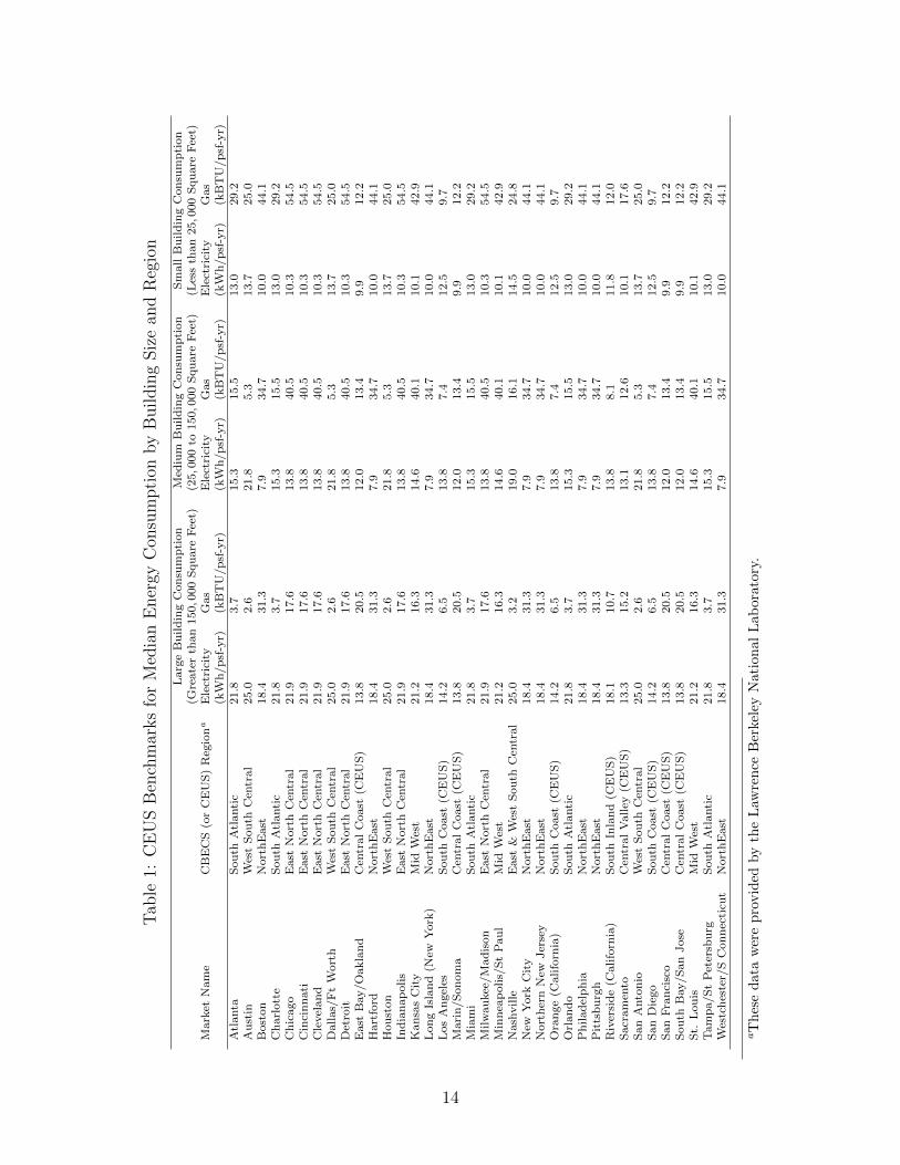
As shown in Table 1, there is considerable variability in the consumption levels of nat-
ural gas and electricity across regions and building types. In general, the western coastal
regions appear to have lower consumption levels of both electricity and natural gas and the
East Coast and Texas locations appear to have higher consumption levels. There are also
important differences across buildings with different square footage. These reported median
energy consumption variables, as will be discussed below, will have important implications
for pricing the relative risk of mortgage across locations and building sizes.
5 Commercial Real Estate Mortgage Valuation with
Energy Risk
As previously discussed, the traditional mortgage valuation process focuses on the dynamics
of interest rates and building prices to model the market price of the mortgage cash flows.
However, to account for energy risk, building prices must be decomposed into market rents
minus total costs including the costs of energy expenditures. The canonical representation
for the market price of a commercial real estate asset is the discounted present value of the
asset’s future net operating income. Since well-maintained office properties typically can
be assumed to be long-lived assets, the market price per square foot of a commercial office
building at the investor’s purchase date (t = 0) can be written as
P (0) =∞∑t=1
E0 [NOI(t)]
(1 + it)t, (1)
13
Tab
le1:
CE
US
Ben
chm
arks
for
Med
ian
Ener
gyC
onsu
mpti
onby
Buildin
gSiz
ean
dR
egio
n
Larg
eB
uild
ing
Con
sum
pti
on
Med
ium
Bu
ild
ing
Con
sum
pti
on
Sm
all
Bu
ild
ing
Con
sum
pti
on
(Gre
ate
rth
an
150,0
00
Squ
are
Fee
t)(2
5,0
00
to150,0
00
Squ
are
Fee
t)(L
ess
than
25,0
00
Squ
are
Fee
t)M
ark
etN
am
eC
BE
CS
(or
CE
US
)R
egio
na
Ele
ctri
city
Gas
Ele
ctri
city
Gas
Ele
ctri
city
Gas
(kW
h/p
sf-y
r)(k
BT
U/p
sf-y
r)(k
Wh
/p
sf-y
r)(k
BT
U/p
sf-y
r)(k
Wh
/p
sf-y
r)(k
BT
U/p
sf-y
r)A
tlanta
Sou
thA
tlanti
c21.8
3.7
15.3
15.5
13.0
29.2
Au
stin
Wes
tS
ou
thC
entr
al
25.0
2.6
21.8
5.3
13.7
25.0
Bost
on
Nort
hE
ast
18.4
31.3
7.9
34.7
10.0
44.1
Ch
arl
ott
eS
ou
thA
tlanti
c21.8
3.7
15.3
15.5
13.0
29.2
Ch
icago
East
Nort
hC
entr
al
21.9
17.6
13.8
40.5
10.3
54.5
Cin
cin
nati
East
Nort
hC
entr
al
21.9
17.6
13.8
40.5
10.3
54.5
Cle
vel
an
dE
ast
Nort
hC
entr
al
21.9
17.6
13.8
40.5
10.3
54.5
Dallas/
Ft
Wort
hW
est
Sou
thC
entr
al
25.0
2.6
21.8
5.3
13.7
25.0
Det
roit
East
Nort
hC
entr
al
21.9
17.6
13.8
40.5
10.3
54.5
East
Bay/O
akla
nd
Cen
tral
Coast
(CE
US
)13.8
20.5
12.0
13.4
9.9
12.2
Hart
ford
Nort
hE
ast
18.4
31.3
7.9
34.7
10.0
44.1
Hou
ston
Wes
tS
ou
thC
entr
al
25.0
2.6
21.8
5.3
13.7
25.0
Ind
ian
ap
oli
sE
ast
Nort
hC
entr
al
21.9
17.6
13.8
40.5
10.3
54.5
Kan
sas
Cit
yM
idW
est
21.2
16.3
14.6
40.1
10.1
42.9
Lon
gIs
lan
d(N
ewY
ork
)N
ort
hE
ast
18.4
31.3
7.9
34.7
10.0
44.1
Los
An
gel
esS
ou
thC
oast
(CE
US
)14.2
6.5
13.8
7.4
12.5
9.7
Mari
n/S
on
om
aC
entr
al
Coast
(CE
US
)13.8
20.5
12.0
13.4
9.9
12.2
Mia
mi
Sou
thA
tlanti
c21.8
3.7
15.3
15.5
13.0
29.2
Milw
au
kee
/M
ad
ison
East
Nort
hC
entr
al
21.9
17.6
13.8
40.5
10.3
54.5
Min
nea
polis/
St
Pau
lM
idW
est
21.2
16.3
14.6
40.1
10.1
42.9
Nash
vil
leE
ast
&W
est
Sou
thC
entr
al
25.0
3.2
19.0
16.1
14.5
24.8
New
York
Cit
yN
ort
hE
ast
18.4
31.3
7.9
34.7
10.0
44.1
Nort
her
nN
ewJer
sey
Nort
hE
ast
18.4
31.3
7.9
34.7
10.0
44.1
Ora
nge
(Califo
rnia
)S
ou
thC
oast
(CE
US
)14.2
6.5
13.8
7.4
12.5
9.7
Orl
an
do
Sou
thA
tlanti
c21.8
3.7
15.3
15.5
13.0
29.2
Ph
ilad
elp
hia
Nort
hE
ast
18.4
31.3
7.9
34.7
10.0
44.1
Pit
tsb
urg
hN
ort
hE
ast
18.4
31.3
7.9
34.7
10.0
44.1
Riv
ersi
de
(Califo
rnia
)S
ou
thIn
lan
d(C
EU
S)
18.1
10.7
13.8
8.1
11.8
12.0
Sacr
am
ento
Cen
tral
Valley
(CE
US
)13.3
15.2
13.1
12.6
10.1
17.6
San
Anto
nio
Wes
tS
ou
thC
entr
al
25.0
2.6
21.8
5.3
13.7
25.0
San
Die
go
Sou
thC
oast
(CE
US
)14.2
6.5
13.8
7.4
12.5
9.7
San
Fra
nci
sco
Cen
tral
Coast
(CE
US
)13.8
20.5
12.0
13.4
9.9
12.2
Sou
thB
ay/S
an
Jose
Cen
tral
Coast
(CE
US
)13.8
20.5
12.0
13.4
9.9
12.2
St.
Lou
isM
idW
est
21.2
16.3
14.6
40.1
10.1
42.9
Tam
pa/S
tP
eter
sbu
rgS
ou
thA
tlanti
c21.8
3.7
15.3
15.5
13.0
29.2
Wes
tch
este
r/S
Con
nec
ticu
tN
ort
hE
ast
18.4
31.3
7.9
34.7
10.0
44.1
aT
hes
ed
ata
wer
ep
rovid
edby
the
Law
ren
ceB
erkel
eyN
ati
on
al
Lab
ora
tory
.
14
where P (0) is the market price per square foot at the investment date, t = 0, E0 [NOI(t)] is
the expected net operating income per square foot at the tth period, and the discount rate for
cash flows at date t, it, equals the riskless rate plus a risk premium. This can alternatively
be written in terms of “risk-neutral” expectations (see Harrison and Kreps, 1979) as
P (0) = E∗0
[∞∑i=1
NOI(i∆t)e−∆t∑i−1
j=0 r̃j ∆t
], (2)
where r̃t is the one-period riskless interest rate at date t. The net operating income per
where c(t)psf is the rent per square foot, (pgas(t)×qgas(t)) is the total gas expense per square
foot (the price pgas(t) per square foot times the quantity of gas used per square foot qgas(t)),
(pelec(t)×qelec(t)) is the total electricity expense per square foot (the price pelec(t) per square
foot times the quantity of electricity used per square foot qelec(t)), and other expenses per
square foot, (pother(t)× qother(t)).The challenge of this decomposition is that the mortgage valuation problem must now
account for the dynamics of four stochastic processes: 1) interest rates; 2) electricity forward
prices at the appropriate geographic hub in which the property is located; 3) gas futures
prices at the Henry Hub; and 4) office market rents for the building that is the collateral on
the loan that is to be priced. A schematic for our proposed modeling strategy is presented
in Figure 3. Moving from left to right in the Figure 3 schematic, our mortgage valuation
protocol requires market specific data for interest rates; electricity prices, natural gas prices,
and office market rents. As previously discussed, the electricity price data is specific to the
electricity hub in which the building is located. We assume that the natural gas dynamics
are determined by the NYMEX Henry Hub futures price dynamics that are common to all
office buildings in the U.S. The interest rate process is also common across all buildings and
the data for this process is U.S. Treasury data. The rental process must be calibrated for
each building, as will be discussed in more detail below.
The data requirements for the augmented mortgage valuation protocol are also significant.
Our valuation protocol requires the interest rate process, the electricity price process, and the
natural gas price process to “match” (exactly fit) the observed term structure of interest rates
or forward contract prices for every month for which we intend to price mortgage contracts.
This requires that we collect monthly data series from 2002 through 2007 corresponding
to the sample of mortgages that we will price. In addition, the natural gas and electricity
15
Figure 3: Flow Chart for the Mortgage Valuation Strategy
I. Simulate Rent
G.B.M.
Hull WhiteProcess
Hull WhiteProcess
Hull WhiteProcess
Rent Data
Power Data
Gas Data
InterestRate Data
µ̂i
II. Price Loans
Solve for the property specific drift, µ̂i
simulations also require information on the expected building specific consumption levels
of natural gas and electricity per square foot. As previously discussed, we use the CEUS
and CBECS benchmarking values by matching buildings to locations and their appropriate
building size.13
As shown in Figure 3, the next component of the valuation protocol is to fit a Hull-White
process for interest rates and exponential Hull-White processes for electricity and natural gas
prices. As will be discussed below, these functional forms are commonly used in modeling
these dynamics in both the practitioner and academic literatures. The price dynamics for
each of the stochastic components of the model are fit exogenously using market data from
each of the respective markets.
In Stage I of the modeling protocol, we solve for the implied risk-neutral drift, µ̂i, of the
building specific market rental process, assumed to be a Geometric Brownian motion (GBM),
conditional on the estimated dynamics of the interest rates, electricity forward prices, and
natural gas forward prices. The solution for this implied drift is the value that will exactly
match the observed price of the building at the origination date of the mortgage given the
market dynamics of the three other market fundamentals. Once the drift parameter of
the building specific rent is optimally fit, the valuation component of the model, the Stage
II component, applies the four stochastic factors: 1) interest rates; 2) electricity forward
13This strategy does not allow the demand for power or natural gas to fluctuate as a function of prices.However, there is considerable evidence that office buildings in the U.S. are sufficiently inefficient that theyare unable to make such price related adjustments.
16
prices; 3) natural gas futures prices; and 4) the market rents for the building in a Monte
Carlo simulation to compute the expected value of the contractual mortgage cash flows and
the value of the embedded default option. To recap the stages of the modeling process:
1. Monthly data are assembled for U.S. interest rates; electricity forward prices by elec-
tricity hub; and natural gas forward prices for the Henry Hub;
2. The interest rate is fit to a Hull-White process and the gas and electricity price data
are fit to exponential Hull-White processes. These processes are fit to exactly match
the observed term structure of these series on a monthly frequency.
3. Stage I : Using the fitted dynamics of interest rates and energy forward prices, the long
run mean, or drift, of the stochastic price process for a building’s market rent dynamic
is fit, assuming that the process follows a GBM, such that the estimated process exactly
matches the observed building price at the origination of the mortgage.
4. Stage II : Using a four factor model (interest rates, natural gas forward prices; electric-
ity hub forward prices, and the building specific rental price dynamic), Monte Carlo
simulation is used to value the mortgage contract cash flows and the embedded default
option.
5.1 Interest Rate Dynamics
In practice for mortgage valuation, interest rate models are fit to observed market data for
the term structure of interest rates and the volatility of interest rates. The Hull and White
(1990) model is a commonly assumed model for this application due to its flexibility in
exactly matching observed term structures and volatilities. In the Hull and White (1990)
model, the short-term riskless rate is assumed to follow the risk-neutral process
dr(t) = (θ(t)− αrr(t)) dt+ σr dW (t), (4)
where dW (t) defines a standard Brownian motion under the risk-neutral measure, and θ(t),
αr, σr and r0 (the starting rate at time zero) are the parameters that need to be estimated.
The function θ(t) is fit so that the model matches the yield curve for the U.S. LIBOR swap
rate on September 30, 2004. Hull and White (1990) show that θ(t) is given by
θ(t) = Ft(0, t) + αrF (0, t) +σ2r
2αr
(1− e−2αrt
),
where F (0, t) is the continuously compounded forward rate at date 0 for an instantaneous
loan at t. Parameters αr and σr are fit with maximum likelihood using U.S. Treasury curve
data and implied caplet volatilities.
17
5.2 Rent Dynamics
The market rent of an office building, as discussed above is assumed to follow a geometric
Brownian motion,
dCt = µ̂Ct dt+ φCCt dWt, (5)
where µ̂ is the risk adjusted long run drift of the rental process and φC is the volatility. The
process defined by equation (5) is fit individually for each building that is the collateral for
each mortgage. The results of this fitting process is will be discussed in detail below. The
estimate for volatility was estimated in Stanton and Wallace (2011) to be φC = 21.478, by
solving for the implied volatility from a large sample of 9,778 office building loans originated
between 2002 and 2007.
5.3 Electricity and Gas Dynamics
We calibrate the dynamics of electricity and natural gas prices following Schwartz (1997)
and Clewlow and Strickland (1999), assuming the log of the spot price for electricity (e) and
natural gas (g) follows a Hull and White (1990) process,
To match the initial forward curve for electricity and futures curve for natural gas, we need
to set
µe,g(t) =∂ lnFe,g(0, t)
∂t+ αe,g lnFe,g(0, t) +
σ2e,g
4αe,g
(1− e−2αe,gt
). (7)
Clewlow and Strickland (1999) show that
Fe,g(t, T ) = Fe,g(0, T )
(Se,g(t)
Fe,g(0, t)
)exp(−αe,g(T−t))
exp
[−σ2e,g
4αe,ge−αe,gT
(e2αe,gt − 1
) (e−αe,gT − e−αe,gt
)].
(8)
In other words, the forward (futures) curve at any future time is simply a function of the spot
price at that time, the initial forward (futures) curve, and the volatility function parameters
for electricity and natural gas, respectively.
5.4 Data and Calibration
The data collection and processing procedures used to construct the needed monthly obser-
vations on electricity and natural gas forward prices by contract maturity are described in
the Appendix.
18
5.4.1 Calibrating the Electricity Forward Curves
In Table 2, we report the estimation for the exponential Hull-White model parameters for
the electricity forward curve. Our objective is to calibrate the parameters αe and σe in
Equation (6), the stochastic differential equation describing the dynamics of the forward
curve for electricity. As a first step, we pre-process the forward prices by tagging, at each
trading date, the number of months out before delivery for each forward price. For example,
the nearest contract (prompt contract) has month out equal to 1, the second to prompt
contract is assigned with month out equal 2 and so forth.
In the pre-processed data, we also keep track of the source package related to the for-
ward price entry. For example, in 12/28/2006 the on-peak PJM Western hub October-2008
contract has its quote derived from an annual package (package length equal 12). The next
trading date, 12/29/2006, the source of the quote is now from a quarterly package (package
length equal 3).
For a given forward price, we then calculate the volatility for each month out. For
example, the on-peak PJM Western hub January-2009 contract has about 22 returns when
it is 10 months out. Its 10-month-out volatility is calculated as the standard deviation of
the 22 daily returns and the result is then annualized. The same on-peak PJM Western
hub January-2009 contract has about 22 return entries when the contract is 9 months out.
We proceed in the same way to calculate its 9-month-out instantaneous volatility. Finally,
we compute the average volatility for each month out and package length. This procedure
allows us to calibrate the term structure of instantaneous historical volatility as a function
of maturity, while controlling for package length. The calibrated parameters αe and σe are
estimating by regressing the logarithm of the average volatilities on month out measured in
years and package length.
As shown in the Table 2, there is considerable heterogeneity across the electricity hubs in
the fitted values of the speed of mean reversion, αe, of the exponential Hull-White process
and in the volatility, σe. The results indicate that overall the higher volatility of forward
prices is higher in the Western time zones than it is in the Eastern times, but it is the highest
for the forward prices observed in the ERCOT hub. The speeds of adjustment to the long
run drift, αe, are not as differentiated by regions as are the volatilities, however, again the
ERCOT hub exhibits a higher speed of adjustment than any of the other over-the-counter
markets. The effects of these differences will become more apparent in our discussion below.
As shown in Figures 4 and 5, we graph a time series of our estimated forward price curves
by the maturity of the contract out to twenty five months of maturity. In Figure 4, we present
the ERCOT and Eastern time zone hubs and, in Figure 5, we present the Western network
hubs. As is clear from these Figures, there is significant heterogeneity in the fitted forward
19
Table 2: Parameter Estimates, αe and σe, of the Exponential Hull-White Process for theElectricity Hubs (Average 2004–2010)
Region αe σeEast New York Zone J 0.352 0.313ERCOT 0.417 0.525Into Cinergy 0.231 0.384Into Entergy 0.363 0.448Into Southern 0.364 0.414Into TVA 0.303 0.424Mass Hub 0.279 0.353Mid-Columbia 0.175 0.489Northern Illinois Hub 0.190 0.437North Path 15 0.236 0.457Palo Verde 0.206 0.473PJM West 0.272 0.347South Path 15 0.212 0.446
price term structures both across hubs and between the Eastern, ERCOT, and Western
networks, although there is more similarities within each power network. As shown, both
the level and the slopes of the fitted forward price curves differ importantly over time. It is
also interesting to note that these markets are often decoupled with some hubs exhibiting
backwardated (downward sloping) forward curves while at the same time the forward curves
for other hubs are in contango (upward sloping). The import differences in the time series
dynamics and in the overall level of prices across the various maturities is also quite signifi-
cant. Overall these curves suggest, that hub-specific heterogeneity in electricity pricing could
potentially drive important differences in the relative default risk of mortgages collateralized
by buildings located across these regions.
Cross-sectional Differences Figure 6 presents a snapshot at four dates: 1) January 1,
2006; 2) April 1, 2008; May 9, 2009; and March 30, 2010; for a cross-section of the fitted
electricity forward curves for all the electricity hubs in the sample. As is clear from these
cross-sections there are some dates, e.g. for May 9, 2009 and March 30, 2010, when the
forward curves have very similar shapes although the level of prices to differ importantly.
Whereas on other dates, e.g. for January 1, 2006, the Western hubs appear to move together
and for other dates, e.g. for April 1, 2008, the ERCOT hub has a significantly different shape
(it is in contango) while the term structure of forward rates for the other hubs are downward
sloping. Again, Figure 6 strongly suggests that the cross-sectional differences in the risk of
electricity exposure should be important in mortgage pricing across regions.
20
05
10
15
20
25
01−
Ma
y−
20
10
01−
Ju
l−2
00
90
1−
Se
p−
20
08
01−
No
v−
20
07
01−
Ja
n−
20
07
01−
Ja
n−
20
06
20
40
60
80
10
0
12
0
Ma
turity
(M
on
ths)
Erc
ot
Da
te
Price ($)
(a)
ER
CO
TH
ub
05
10
15
20
25
01−
Ma
y−
20
10
01−
Ju
l−2
00
90
1−
Se
p−
20
08
01−
No
v−
20
07
01−
Ja
n−
20
07
01−
Ja
n−
20
06
20
40
60
80
10
0
12
0
Ma
turity
(M
on
ths)
PJM
We
st
Da
te
Price ($)
(b)
PJM
Wes
tH
ub
05
10
15
20
25
01−
Ma
y−
20
10
01−
Ju
l−2
00
90
1−
Se
p−
20
08
01−
No
v−
20
07
01−
Ja
n−
20
07
01−
Ja
n−
20
06
40
60
80
10
0
12
0
14
0
16
0
18
0
Ma
turity
(M
on
ths)
Ea
st
Ne
w Y
ork
Zn
J
Da
te
Price ($)
(c)
Eas
tN
ewY
ork
Zon
eJ
Hu
b
05
10
15
20
25
01−
Ma
y−
20
10
01−
Ju
l−2
00
90
1−
Se
p−
20
08
01−
No
v−
20
07
01−
Ja
n−
20
07
01−
Ja
n−
20
06
20
40
60
80
10
0
Ma
turity
(M
on
ths)
Into
Cin
erg
y
Da
te
Price ($)
(d)
Into
Cin
ergy
Hu
b
Fig
ure
4:F
itte
dE
lect
rici
tyForw
ard
Curv
es,
2006–2010.
This
figu
replo
tsou
rca
libra
ted
elec
tric
ity
forw
ard
curv
esfo
ra
sele
ctio
nof
the
ER
CO
Tan
dE
aste
rnel
ectr
icit
yhubs.
We
plo
tth
efo
rwar
dcu
rve
per
mon
thby
the
mat
uri
tyof
the
contr
act.
21
05
10
15
20
25
01−
Ma
y−
20
10
01−
Ju
l−2
00
90
1−
Se
p−
20
08
01−
No
v−
20
07
01−
Ja
n−
20
07
01−
Ja
n−
20
06
20
40
60
80
10
0
12
0
Ma
turity
(M
on
ths)
Pa
lo V
erd
e
Da
te
Price ($)
(a)
Pal
oV
erd
eH
ub
05
10
15
20
25
01−
Ma
y−
20
10
01−
Ju
l−2
00
90
1−
Se
p−
20
08
01−
No
v−
20
07
01−
Ja
n−
20
07
01−
Ja
n−
20
06
20
40
60
80
10
0
12
0
14
0
Ma
turity
(M
on
ths)
So
uth
Pa
th 1
5
Da
te
Price ($)
(b)
Sou
thP
ath
15
Hu
b
05
10
15
20
25
01−
Ma
y−
20
10
01−
Ju
l−2
00
90
1−
Se
p−
20
08
01−
No
v−
20
07
01−
Ja
n−
20
07
01−
Ja
n−
20
06
20
40
60
80
10
0
12
0
14
0
Ma
turity
(M
on
ths)
No
rth
Pa
th 1
5
Da
te
Price ($)
(c)
Nor
thP
ath
15H
ub
05
10
15
20
25
01−
Ma
y−
20
10
01−
Ju
l−2
00
90
1−
Se
p−
20
08
01−
No
v−
20
07
01−
Ja
n−
20
07
01−
Ja
n−
20
06
20
40
60
80
10
0
12
0
Ma
turity
(M
on
ths)
Mid−
Co
lom
bia
Da
te
Price ($)
(d)
Mid
Colu
mb
iaH
ub
Fig
ure
5:F
itte
dE
lect
rici
tyForw
ard
Curv
es,
2006–2010.
This
figu
replo
tsou
rca
libra
ted
elec
tric
ity
forw
ard
curv
esfo
ra
sele
ctio
nof
the
Wes
tern
elec
tric
ity
hubs.
We
plo
tth
efo
rwar
dcu
rve
per
mon
thby
the
mat
uri
tyof
the
contr
act.
22
020406080100
120 Ju
l/06
Oct/06
Jan/07
Apr/07
Aug/07
Nov/07
Feb/08
Jun/08
Sep/08
Dec/08
East NY ZnJ
ERCO
TInto Cinergy
Into Entergy
Into Sou
thern
Into TVA
Mass Hub
Mid‐Col
NI H
ubNorth Path 15
Palo Verde
PJM W
est
South Path 15 (a
)Jan
uar
y1
2006
020406080100
120
140 Feb/08
Jun/08
Sep/08
Dec/08
Mar/09
Jul/09
Oct/09
Jan/10
May/10
Aug/10
East NY ZnJ
ERCO
TInto Cinergy
Into Entergy
Into Sou
thern
Into TVA
Mass Hub
Mid‐Col
NI H
ubNorth Path 15
Palo Verde
PJM W
est
South Path 15
(b)
Ap
ril
1,
2008
0
10
20
30
40
50
60
70
80
90
100
0.0
0.5
1.0
1.5
2.0
2.5
East NY ZnJ
ERCOT
Into Cinergy
Into Entergy
Into Southern
Into TVA
Mass Hub
Mid‐Col
NI H
ub
North Path 15
Palo Verde
PJM
West
South Path 15
(c)
May
9,20
09
01020304050607080
Jan/10
May/10
Aug/10
Nov/10
Feb/11
Jun/11
Sep/11
Dec/11
Apr/12
Jul/12
East NY ZnJ
ERCO
TInto Cinergy
Into Entergy
Into Sou
thern
Into TVA
Mass Hub
Mid‐Col
NI H
ubNorth Path 15
Palo Verde
PJM W
est
South Path 15 (d
)M
arc
h30,
2010
Fig
ure
6:C
ross
-Sect
ion
of
Fit
ted
Ele
ctri
city
Forw
ard
Curv
es
acr
oss
the
Ele
ctri
city
Hubs
on
Sp
eci
fic
date
s.T
his
figu
repre
sents
acr
oss
sect
ion
offo
rwar
dcu
rves
for
each
hub
ona
singl
edat
e.
23
Characteristics of Volatility As was discussed previously, there is considerable volatility
in electricity price dynamics. In Figures 7 and 8, we graph a cross-sectional comparison for
the historical volatilities by maturity for the forward contracts up through November 2007.
The Figures plot both the observed level of volatility by maturity and a fitted term structure
of volatility. As volatility is an important determinant of the value of embedded mortgage
default options, it is interesting to again note the important cross-sectional differences in the
level and the slopes of these term structures. Interestingly, as shown in Figure 7 the level of
volatility at the short maturity contracts is considerably higher than that for the Eastern time
zone hubs. The ERCOT hub exhibits the highest volatility in the short maturity contracts
across all of the hubs. Here again, these results suggest important potential differential in
the expected value of embedded mortgage default options for mortgage written on building
located across these hubs. As shown, these volatility levels exceed the volatility of rents, φC
= 21.478%, and that of interest rates is about σr = 2.21% (see Veronesi, 2010).
5.4.2 Calibrating the Natural Gas Futures Curves
As previously discussed, there is only one major pricing hub for natural gas, the Henry Hub.
As for the electricity hubs, we estimate the parameters for the exponential Hull-White process
using data from Henry Hub NYMEX futures and options on NYMEX futures contracts. The
time series average from 2004 through 2010 for αg is 79.1% (standard deviation, 3.7%) and
is 58.7% (standard deviation, 1.4%) for σg. These values are again importantly larger than
the volatility values for either the interest rate or building rent process.
Time Series Dynamics In Figure 9, we graph the NYMEX Henry Hub futures contract
curves over time from 2006 through 2010. As shown there is significant times series variation
in the shape and level of the natural gas futures price curve as a function of the maturity
of the contracts. Again, the curves are backwardated in some periods and in contango in
others.
Implied Volatility In contrast with the electricity markets, we were able to gain access to
a third-party dataset describing the term structure of at-the-money (ATM) implied volatili-
ties of NYMEX Henry Hub futures contracts on a daily basis over the analysis period. This
third-party dataset was built by backing out implied volatilities from market quotes of put
and call option premia with strike prices near to the closing prices of the underlying futures
contracts. Implied volatilities for near to ATM strikes were derived from straight applica-
tion of the Black (1976) option pricing formula for futures contracts. The ATM implied
volatilities were constructed by interpolation across nearby strikes.
24
0%5%10%
15%
20%
25%
30%
35%
40%
45%
50%
010
2030
4050
6070
Mon
ths
Out
(a)
Pal
oV
erde
Hu
b
0%10%
20%
30%
40%
50%
60%
010
2030
4050
6070
Mon
ths
Out
(b)
Sou
thP
ath
15
Hu
b
0%5%10%
15%
20%
25%
30%
35%
40%
45%
50%
010
2030
4050
6070
Mon
ths
Out
(c)
Nor
thP
ath
15H
ub
0%10%
20%
30%
40%
50%
60%
010
2030
4050
6070
Mon
ths
Out
(d)
Mid
Colu
mb
iaH
ub
Fig
ure
7:C
ross
-Sect
ion
of
His
tori
cal
Vola
tili
ties
by
Matu
rity
of
the
Forw
ard
Contr
act
on
Novem
ber
11,
2007.
This
figu
replo
tsth
ehis
tori
cal
vola
tiliti
esfo
ra
sele
ctio
nof
the
Wes
tern
Hubs.
The
dot
ted
curv
eis
the
com
pute
dhis
tori
cal
vola
tility
for
the
forw
ard
contr
acts
ofgi
ven
mat
uri
ties
.T
he
solid
line
plo
tsth
efitt
edvo
lati
lity
curv
e.
25
0%10%
20%
30%
40%
50%
60%
70%
010
2030
4050
6070
Mon
ths
Out
(a)
ER
CO
T
0%5%10%
15%
20%
25%
30%
35%
40%
010
2030
4050
6070
Mon
ths
Out
(b)
PJM
East
Hu
b
0%5%10%
15%
20%
25%
30%
35%
40%
010
2030
4050
6070
Mon
ths
Out
(c)
Eas
tN
ewY
ork
Zon
eJ
Hu
b
0%5%10%
15%
20%
25%
30%
35%
40%
010
2030
4050
6070
Mon
ths
Out
(d)
Mid
Colu
mb
iaH
ub
Fig
ure
8:C
ross
Sect
ion
of
His
tori
cal
Vola
tili
ties
by
Matu
rity
of
the
Forw
ard
Contr
act
on
Novem
ber
11,
2007.
This
figu
replo
tsth
ehis
tori
cal
vola
tiliti
esfo
ra
sele
ctio
nof
the
ER
CO
Tan
dE
aste
rnH
ubs.
The
dot
ted
curv
eis
the
com
pute
dhis
tori
cal
vola
tility
for
the
forw
ard
contr
acts
ofgi
ven
mat
uri
ties
.T
he
solid
line
plo
tsth
efitt
edvo
lati
lity
curv
e.
26
Figure 9: Estimated NYMEX Henry Hub Futures Contract Curves
05
1015
2025
01−Mar−201001−May−2009
01−Jul−200801−Sep−2007
01−Nov−200601−Feb−2006
2
4
6
8
10
12
14
Maturity (Months)
Nymex HH Futures
Date
Pric
e ($
/ M
MBt
u)
27
From Black (1976), the implied volatility defines the variance of terminal future prices
through the relationship
V art [lnFg(t, T )] = σg2(T − t), (9)
with σg expressing the implied volatility.
Also, from the stochastic equation for futures contracts, we express the terminal variance
of the logarithm of the futures price at maturity as
V art [lnFg(t, T )] =
∫ T
t
σ2ge−2αg(T−u)du =
σ2g
2αg
[1− e−2αg(T−t)] (10)
By combining equations (9) and (10), the implied volatility is then expressed as
σg =
√σ2g
2αg(T − t)[1− e−2αg(T−t)]. (11)
Although we were not able to characterize seasonal patterns in the term structure of
instantaneous volatility for the electricity markets, we were able to do so for the natural gas
markets. We identified the seasonal pattern by simply averaging the implied volatility by
contract month (1 = January, 12 = December) over the whole time period.
For each trading date, the parameters αg and σg are calibrated by minimizing the sum
of squares of the residuals of the term structure of ATM implied volatilities. We fit a curve
of the form
σg(t, T ;m) =
√(σg × sfm)2
2αg(T − t)[1− e−2αg(T−t)], (12)
where m is the month of expiration of the futures contract and sfm is the corresponding
seasonal scaling factor tabulated above.
Figure 10 and Figure 11 plot the term structure of implied volatilities from options
on NYMEX futures contracts on November 1, 2007 and for November 2, 2009. We plot
the observed non-seasonally adjusted implied volatilities (the red plot); the non-seasonally
adjusted fitted term structure of volatility (the blue plot); and the de-seasonalized fitted
term structure of volatilities (the black plot) for the two dates. As shown in Figure 10
and Figure 11, there is considerable heterogeneity in the implied volatilities across option
maturities at short maturities, but the curves fall to about the same level of implied volatility
for the longer maturity options. Nevertheless, these volatilities are comparable to those of
the electricity hubs and importantly exceed the levels of either interest rate volatility or the
volatility of office rents.
28
Figure 10: NYMEX Natural Gas Implied Volatilities, November 1, 2007
0%
10%
20%
30%
40%
50%
60%
70%
80%
0 5 10 15 20 25 30 35 40 45 50 55 60months out
Implied Volatility Curve imp_vol Sz Fit
Figure 11: NYMEX Natural Gas Implied Volatilities, November 1, 2009
0%
10%
20%
30%
40%
50%
60%
70%
80%
0 5 10 15 20 25 30 35 40 45 50 55 60months out
Implied Volatility Curve imp_vol Sz Fit
29
6 Two-Part Valuation Strategy
Overall, the fitted factor dynamics for interest rates, energy forward prices, and rents sug-
gest that the energy prices could induce important volatility into cash flows and, therefore
into building prices over time. Since commercial mortgage are long contracts, these results
indicate that the volatility of energy costs to the building owner could swamp other costs
such as janitorial services and the cost of building management staff.
6.1 Part I: Solving for Building-Specific Rental Drift
In order to obtain reliable mortgage values, it is important first to ensure that the valuation
model we are using is consistent with the current price of the underlying building. As
previously discussed, therefore, in Stage I of the valuation strategy on a given date, we fit
the interest rate process, the electricity forward process, and the natural gas futures process,
then solve for the implied building-specific, risk-adjusted drift for market rents, µi, assuming
a volatility of 21.478% (see Stanton and Wallace, 2011). The implied drift is the value that
makes the valuation model exactly match the observed price of the building at the origination
date of the mortgage, given the market dynamics of the three other market fundamentals.
Valuation of the building is performed using Monte Carlo simulation with antithetic
variates to estimate the price as the (risk-neutral) expectation of future cash flows,14
Pt = E∗t
[∞∑k=1
CFt+k∆te−∆t
∑k−1j=0 r̃t+j ∆t
]. (13)
Estimating the expectation in Equation (13) involves three steps:
1. Simulate 10,000 paths for rent, interest rates, gas prices, and electricity prices using
the risk-neutral processes described above.
2. Calculate the monthly building cash flow (NOI) along each path from Equation (3).
3. Discount each path’s cash flows back to the present, and average across all paths.
We repeat this process for various different values of µ̂ in Equation (5), searching numerically
until we find the value that makes the building price produced by the Monte Carlo valuation
equal to the known price of the building at the mortgage origination date.15
14For details see, for example, Boyle (1977); Boyle, Broadie, and Glasserman (1997); Glasserman (2004).15In performing this search, it is important to use the same set of random numbers for each valuation.
30
6.2 Part II: Solving for Mortgage Value
Valuing mortgages mortgage using Monte Carlo is very similar to the process described above
for calibrating the risk-neutral drift. Specifically, we start by writing the mortgage value as
the risk-neutral expected present value of its future cash flows using Equation (13) again.
Then we use Monte Carlo simulation to estimate the expectation the same way as above.
1. Simulate 10,000 paths for rent, interest rates, gas prices, and electricity prices using
the risk-neutral processes described above.
2. Calculate the monthly cash flows for the mortgage along each path.
3. Discount each path’s cash flows back to the present, and average across all paths.
While structurally similar, there are two significant differences between the two valuations,
both related to step 2, the calculation of the mortgage cash flows along each path:
1. Commercial mortgages include embedded default options, and when borrowers exercise
these options, this affects both the amount and the timing of the mortgage cash flows.
To model the borrowers’ default behavior, we therefore introduce an empirical hazard
model, a model for the estimated conditional probability that a mortgage will default
given its survival times, into Stage II.
2. Because the likelihood of default at any instant depends on the loan-to-value ratio
(LTV), we need a way to estimate the building’s value not just at the mortgage origi-
nation date, but rather at every date along every path.
We now discuss each of these differences in detail.
6.2.1 Empirical Default Hazard Model
Following standard mortgage-valuation practice (see Schwartz and Torous, 1989), the default
hazard for the loans is estimated using a time-varying-covariate hazard model with a log-
logistic baseline hazard.16 Our model also includes controls for loan characteristics including
the amortization structure, the loan coupon, amortizing maturity of the loan, the principal
due date on the loan, the time varying loan-to-value ratios of the building, and a measure of
the difference between the coupon on the loan and the time varying 10 year Treasury rate
which is the measure for current interest rates.
We estimate the proportional-hazard model using a sample of 8,497 loans on commercial
office buildings that were originated between 2002 and 2007. These data were obtained
from Trepp LLC loan-level performance data and include all the origination information on
16For details on hazard models see, for example, Cox and Oakes (1984).
31
Table 3: Office Loan-level Estimates for the Default Hazard
Coeff. Est. Std. Err.
γ 0.0019∗∗∗ 0.00026p 1.94387∗∗∗ 0.0898Current Coupon minus Treasury(t) 0.1613∗∗ 0.04561Loan-to-Value Ratio(t) 0.5771∗∗ 0.02225Number of Observations 8,497t statistics in parentheses∗ p < 0.10, ∗∗ p < 0.05, ∗∗∗ p < 0.01
the mortgages along with monthly performance records. The estimated hazard rate is the
conditional probability that a mortgage will terminate in the next instant, given that it has
survived up until then. Hazard models comprise two components: 1) a baseline hazard that
determines the termination rates simply as a function of time and 2) shift parameters for the
baseline defined by the time-varying evolution of exogenous determinants of prepayment and
default. We define default as a 90-day delinquency on the loan, and model its occurrence
via the hazard function
π(t) = π0(t)eβν , where (14)
π0(t) =γp(γt)p−1
1 + (γt)p. (15)
The first term on the right-hand side of Equation (14) is the log-logistic baseline hazard,
which increases from the origination date (t = 0) to a maximum at t = (p−1)1/p
γ. This is
shifted by the factor eβν , where β is a vector of parameters and ν a vector of covariates
including the end-of-month difference between the current coupon on the mortgage and U.S.
Treasury rates and the current loan-to-value ratio of the mortgage.
The results of our hazard models are reported in Table 3. As expected, there is a
statistically significant, positive coefficient on the difference between the coupon rate on the
mortgage and the observed 10 year Treasury rate and a statistically significant and large
positive coefficient on the current loan-to-value ratio of the loan. Thus, our empirical hazard
suggests that loans will default when the difference between the coupon on the loan and
the current 10 year U.S. Treasury rate is large and, reasonably, when the value of the loan
relative to the value of the building is high.
32
6.2.2 Empirical Building Value Estimator
In order to estimate default rates along each path, we need an estimate of the building value
at every time along each path. In principle, we could just perform a new simulation at
every time step along every path, but this would be computationally infeasible. Instead,
therefore, we construct an empirical model for building value as a function of current NOI,
interest rates and other variables. This is similar to Boudoukh, Richardson, Stanton, and
Whitelaw (1997), who used nonparametric regression to estimate the value of mortgage-
backed securities as a function of interest rates.17 Assuming a constant expected growth
rate for NOI per square foot and a flat term structure of risk-adjusted discount rates the
value, P (t), of an office building per square foot would be given by the Gordon growth model
(in logs),
lnP (t) = lnNOI(t)− ln(i− g), (16)
where g is the market growth rate for net operating income, i is the risk-adjusted discount
rate, and we assume i− g > 0. This is the basis of our empirical valuation estimator, which
we adjust via the inclusion of other explanatory variables.
Based on Equation (16), we fit the following estimator for building values:
where lnP (t) is the natural log of the price per square foot of the building on the transaction
month t, lnNOI(t) is the natural log of the annual net operating income per square foot
on the transaction month t, ln i(t) is the natural log of the ten-year Treasury rate for the
transaction month t, pgas(t) is the average spot price of gas per kBTU for the transaction
month t, and qgas is the annual benchmark level of natural gas consumption (kBTU) per
square foot for buildings of a corresponding size and location to those reported in Table 1,
pelec(t) is average spot price per kWh of electricity for the transaction month t, and qelec is
the annual benchmark level of electricity consumption (kWh) per square foot for buildings
of a corresponding size and location to those reported in Table 1.
To estimate our building value estimator, we construct a data set that combines two
separate transaction data sets: 1) the CoStar Group data; 2) the Trepp LLC data. The
Costar data is a comprehensive data set that is maintained by leasing and sales brokers
in commercial real estate industry. The data offers comprehensive coverage of transactions
17We also use this model in the drift calibration. We simulate out to year 10, then use the empiricalvaluation model to estimate the building’s “terminal value” in year 10. This is similar to the use of short-cutmethods such as valuation multiples in estimating the terminal value when valuing a business (see Berk andDeMarzo, 2007).
33
across the U.S., although its best geographic coverage is for Western States. We use only
the CoStar transactions that are arms-length and confirmed market transactions.18 The
data also include information on the overall building characteristics (building and lot square
footage, typical floor area square footage, numbers of floors, etc), how many tenants, the
location, and quality characteristics of the building, information on the first and second
lien amounts, and the lien periodic payment amounts. For a subset of these data, there
is also information on the annual net operating income at sale, the gross rent at sale, and
the operating expenses at sales. We then further restricted our sample to the transactions
for which we have complete information on transaction characteristics as well as complete
information on the annual net operating income at sale, the gross income at sale, and the total
annual expenses at sale. This further restriction generated a sample of 1,540 observations
from the CoStar transaction data.
Our second data set is obtained from Trepp LLC. Trepp is a data vendor widely regarded
as the most accurate source of data on the securitized commercial loan market in the U.S.
We restricted the Trepp commercial loan data to those loans that were for transactions and
for which we had information on the annual net operating income at sale, the gross rent at
sale, and the operating expenses at sales. This restriction leaves us 3,551 transactions. One
limitation of the Trepp data is that we only have the underwritten appraised value of the
building at the loan origination, rather than the true sales prices. We therefore assume that
the appraised value is the market price of the office building. As shown in Table 4 the two
samples are not that different. Trepp has slightly more expensive buildings, however, the
sample distributions for the revenues and operating expenses levels are comparable for the
two data sources. Given this comparability we merge the two data sets together for a total
transactions data set of 5,092 observations.
As shown in Table 4 the two data set are quite comparable in revenues and expenses per
square foot. The sample of Trepp transactions appear to have sold for a slightly higher price
that those of CoStar. We consider this differences, however, to be minor and we proceed
to fit our building value estimator on the joint sample of 5,091 office transactions. The
summary statistics for the merged transaction data are presented in Table 5. As shown
in Table 5 overall these are fairly large office buildings with an average transaction price
of about $195 per square foot. Annual rents were averaged about $22 per square foot
and annual operating expenses averaged about $7.7 per square foot. The electricity and
18We eliminate all transactions for which there was a “non-arms-length” condition of sale due to suchfactors as a 1031 Exchange, a foreclosure, a sale between related entities, a title transfer, among otherconditions. All of these sale conditions would affect prices due to the trading of tax basis in the case of 1031exchanges or the auction structure in the case of foreclosure. Instead, we focus only on market transactionsbetween unrelated persons.
Variable N Mean Std. Deviation Minimum MaximumAnnual Price ($ per Square Foot) 5091 195.81 104.44 6.04 872.30Annual Revenue ($ per Square Foot) 5091 22.03 9.20 10.00 169.55Annual Expenses ($ per Square Foot) 5091 7.72 3.94 1.00 76.89Ten Year Treasury Rate (%) 5091 4.50 0.00 2.90 5.28Gas Spot Price ($ per kBTU) 5091 0.01 0.00 0.00 0.01Electricity Spot Price ($ per kWh) 5091 0.07 0.02 0.03 0.16Building Size (Square Feet) 5091 100350.34 127589.63 15575.00 998770.00Annual Electricity Consumption (kWh per Square Foot) 5091 1.19 0.35 0.42 3.20Annual Gas Consumption (kBTU per Square Foot) 5091 6.53 3.89 0.01 75.81
gas consumption information for each building was obtained from the CEUS and CBECS
benchmark information provided in Table 1 and discussed above.
The results of estimating our building value estimator are reported in Table 6. As shown,
the estimator explains about 68% of the observed variance in building prices in the same. As
expected the log of net operating income has a statistically significant and positive effect on
log price per square foot and the log of the 10 year Treasury rate has a statistically significant
and negative effect on log price per square foot. We include the additional covariates to
capture the additional effects of energy costs on building transactions prices per square foot.
As shown in Table 6, we find that the log of natural gas and electricity prices have a positive
effect on log price and the benchmarked consumption levels of gas and electricity for buildings
have a negative effect on log prices.
7 Valuation Application
Following Figure 3, the valuation of a specific loan requires data for the market term structure
of interest rates and volatility, the market energy and natural gas forward curves and their
volatility, and the calibrated market rent process for the building. These data need to be
35
Table 6: Estimation Results for the Office Building Valuation using the Trepp and CoStarMerged Data
Coefficient StandardVariable Estimate ErrorIntercept 2.760∗∗∗ 0.068Natural Log of Net Operating Income per square foot 0.898∗∗∗ 0.010Natural Log of the 10 Year Treasury Rate -7.100∗∗∗ 1.168Natural log (Gas Spot Price × Gas Consumption) -0.071∗∗∗ 0.009Natural log (Electricity Spot Price × Electricity Consumption) -0.201∗∗∗ 0.017R2 0.690Includes city fixed effectst statistics in parentheses∗ p < 0.10, ∗∗ p < 0.05, ∗∗∗ p < 0.01
collected for the same date, since the model is pricing the mortgage relative to current
market data. Usually, the date that would be selected would be the mortgage origination
date, however, the modeling strategy could be applied to value the mortgage contract at
any point prior to its maturity. Typically, at origination, the lender is seeking to select the
contractual features of the commercial loan such that its market price, given observed market
fundamentals, is equal to the amount of principal borrowed. Thus, the lender typically
structures the contract so that its market price at origination is equal to par.19
7.1 Loan Valuation Results
To implement our valuation strategy, we first find all of the loans in the Trepp LLC data
set that were originated in September 2004. There were thirteen such loans, and we have
CEUS/CBECS natural gas and electricity consumption data for the cities in which these
loans were originated. We then fit the Hull-White model for the term structure of interest
rates on that date and obtain the estimated values of αr = .128 and σr = 0.12. Similarly,
we use the location of the loan to identify the appropriate electricity forward curve for
September 2004. These are presented in Table 7. As shown in Table 7, even in this small
sample the differences between the hubs is quite apparent. We also fit the forward curve for
natural gas NYMEX futures and options at the Henry Hub in September 2004, obtaining a
value of 0.512 for σg and 0.837 for αg. Finally, conditional on the fitted dynamics of interest
rates and the electricity and natural gas forward prices, we fit the drift of the GBM for the
building specific rent processes for each loan in Stage I of the valuation strategy. These are
19That is the ratio of the market price of the discounted cash flows mortgage net the embedded optionvalues to the principal on the loan is equal to one hundred percent.
36
Table 7: Historical Averages of αe and σe, for the Exponential Hull-White Electricity Processfor the Thirteen Loan Sample
Electricity Hub Network αe σeERCOT Texas Interconnected System 0.42 0.53East NY Zone J Eastern Interconnected System 0.35 0.31Into Cinergy Eastern Interconnected System 0.23 0.38Into TVA Eastern Interconnected System 0.30 0.42North Path 15 Eastern Interconnected System 0.24 0.46South Path 15 Eastern Interconnected System 0.21 0.45
reported in Table 9.
To implement our model, we need information on each of the key contract elements for
every loan that will be modeled. As shown in Table 8, across the thirteen loans there is
considerable variety in the building square footage, the value of the building, the size of
the loan, the coupon rates, and the loan-to-value ratios. Several of the buildings are in a
common electricity hub, so that even in this small sample we can compare across hubs and
across buildings and loans with differing characteristics. As reported in Table 8, the loans
are quite similar in their amortization maturities and in their balance-due maturities. Not
surprisingly, because these loans were all originated in the same month, they have quite
similar coupons although the loans with higher loan-to-value ratios appear to have higher
coupons, as expected, and loans on large buildings have higher coupons. Overall, the loans
are collateralized by large buildings. The average building size is about eighty-nine thousand
square feet with a standard deviation of about fifty three thousand square feet. The average
building price of the thirteen-loan sample is about $13 million, with a standard deviation of
about $7.4 million. The minimum building price in the sample is $4.4 million. As is clear
from Table 8, the expected energy consumption by region is highly variable.
We carry out three simulation exercises for each loan:
1. We value the loan conditional on the dynamics of interest rates, rents, and energy prices
but without default risk. Thus, this pricing exercise values the contractual features of
the loan and compares their present value with the observed balance on the loan. The
idea behind this analysis is that the discounted present value of the loan at origination
should equal the balance on the loan at origination if the loan was fairly priced. This
valuation exercise, of course, ignores the default risk of the mortgages so we expect our
model should price at a premium compared to the balance of the loan since the actual
loan should have been structured to account for the risk of default.
2. In the second set of simulations we allow the mortgages to default. However, we do
not enable the energy channels. Instead, we follow the traditional modeling procedure
37
of accounting for only the rent and interest rate dynamics in valuing a commercial
mortgage contract with an embedded default option.
3. In the third set of simulations for each loan, we enable the energy channel. Here
again we allow for mortgage default. In this set of simulations, our mortgage valuation
strategy accounts for the dynamics of power and natural gas in valuing the commercial
mortgage contract with an embedded default option.
We report the results of our mortgage valuations in Table 9. In the second, third and
fourth columns of the Table 9, we report the geographic location of the loan and its electricity
hub. In the fifth through seventh columns of Table 9, table we report the initial loan-to-
value ratio, the building square footage, and the building value at the origination of the loan.
In column eight, we report the Stage I estimate of the risk adjusted drift of rents for the
building.
The simulation results are reported in the last three columns of Table 9. As shown, on
average, the estimated value of the loans when default is not enabled is quite close to the
observed balance on the loans at origination in September 2004. This result appears, at face,
surprising because it suggests that lenders were, generally, underpricing the default options
on these loans at the time these loans were originated.20
In column 10 of Table 9, we report the results of explicitly pricing the default option
in the thirteen loans originated in September 2004 using the traditional mortgage valuation
methodology, which controls for the effects of rent and interest rate dynamics to value the
embedded default options. As shown, the default options embedded in these mortgage are
valuable and all of the loans appear to be worth significantly less than the balance of the
loans at origination. An important caveat is that our hazard function (see Table 3 for the
coefficient estimates) is estimated using loan-level performance data from 2002 through 2010.
These data include a higher incidence of 90-day delinquencies, our proxy for default, than
would have been forecasted using available loan-level mortgage data prior to the origination
date of these loans. Thus, our model is forecasting more default than lenders could have
forecasted using the same model prior to September 2004, simply because the incidence
of mortgage delinquencies in earlier vintages of commercial mortgages were nearly nonex-
istent. Nevertheless, for the purposes of the simulations reported here, the elevated levels
of forecasted default is useful because it allows us to highlight the differences in mortgage
valuations that are obtainable from using a two-factor versus a four-factor valuation model.
Our results should, however, not be interpreted to mean that on average lenders were ex ante
20At the time these loans were originated the historical default levels (from 1996 through 2004) for secu-ritized commercial mortgages were less than 4%. Thus, the empirical hazard models that were implementedduring this period predicted de minimis levels of expected default and the forecasted value of commercialmortgages was essentially the discounted present value of the default-free contract cash flows.
38
Tab
le8:
Sum
mar
ySta
tist
ics
for
the
Char
acte
rist
ics
ofth
eT
hir
teen
Mor
tgag
esU
sed
inth
eSim
ula
tion
s,Sep
tem
ber
2004
An
nu
alA
nnu
al
Annu
al
An
nu
al
Loan
toL
oan
Ori
gin
atio
nE
lect
rici
tyG
asG
ross
Non
-En
ergy
Bala
nce
Valu
eB
uil
din
gL
oan
Bu
ild
ing
Nu
mb
erD
ate
Con
sum
pti
onC
onsu
mp
tion
Ren
tsE
xp
ense
sM
atu
rity
Du
eR
ati
oP
rice
Cou
pon
Siz
e(k
Wh
/psf
-yr)
(kB
TU
/p
sf-y
r)($
psf
)($
psf
)(M
onth
s)(M
onth
s)(%
)($
000)
(%)
(000
Sqft
)L
oan
1S
ept.
2004
13.8
40.5
13.7
3.7
8360
120
74.0
7,6
10.0
5.7
70.7
Loa
n2
Sep
t.20
0413
.840
.510.4
3.4
8360
120
76.2
8,0
00.0
5.6
124.9
Loa
n3
Sep
t.20
0418
.431
.319.2
7.8
7360
120
77.1
22,0
00.0
5.8
176.2
Loa
n4
Sep
t.20
0418
.431
.317.1
5.9
3120
120
59.5
21,5
00.0
5.3
206.4
Loa
n5
Sep
t.20
0413
.87.
421.6
6.7
360
120
67.9
9,5
60.0
5.9
41.6
Loa
n6
Sep
t.20
0413
.87.
424.4
8.4
3360
122
74.8
16,2
00.0
5.5
77.0
Loa
n7
Sep
t.20
0415
.315
.510.2
2.7
6360
120
74.8
12,0
00.0
5.6
123.4
Loa
n8
Sep
t.20
0413
.88.
116.0
5.3
2360
120
65.2
11,1
00.0
6.2
82.4
Loa
n9
Sep
t.20
0413
.112
.623.3
5.1
7360
120
77.9
14,3
50.0
5.8
71.5
Loa
n10
Sep
t.20
0413
.112
.616.5
2.9
6360
120
78.7
6,3
50.0
5.7
41.1
Loa
n11
Sep
t.20
0410
.117
.621.3
5.9
9360
120
70.9
4,3
60.0
5.9
24.1
Loa
n12
Sep
t.20
0421
.85.
318.6
5.8
3300
120
61.4
6,0
00.0
6.1
43.3
Loa
n13
Sep
t.20
0412
.013
.425.3
6.5
4240
240
69.3
27,0
00.0
5.5
123.8
Ave
rage
14.7
18.7
18.3
5.4
327.7
129.4
71.4
12,7
71
5.7
92.8
Sta
nd
ard
Dev
iati
on3.
012
.24.7
1.7
69.1
31.9
6.1
6,7
88.0
0.3
53.0
39
mispricing the default options in these thirteen loans. We now know ex post that this was
true, however, the point of our exercise is to shown that ex ante the traditional mortgage
valuation methodology would have mispriced the loans because it ignores the effect of energy
price dynamics on the value of commercial mortgage default.
The results of valuing the thirteen mortgages, again as of their origination date in
September 2004, using the full four-factor mortgage valuation model, are reported in column
11 of Table 9. As shown in Table 9, the inclusion of the energy channels generates mortgage
values that are now on average about 8.89% below the value of the mortgages using the
traditional modeling approach (which ignores the energy channel in valuing the embedded
default options). For the most part these valuation reductions are larger for mortgages that
are collateralized by larger buildings (which exhibit higher energy consumption on average)
and mortgages with higher loan-to-value ratios. For some of the smaller buildings the ef-
fects are significantly smaller. Ignoring the dynamics of the energy factor inputs would lead
lenders to significantly misprice the default risk of mortgages. On average, in the Trepp
loan origination data, gas and electricity benchmarked expenditures represent about 19%
of observed overall expenditures per square foot. Our results suggest that by not explic-
itly accounting for the important volatility of the energy related expenditures would lead to
important overall levels of expected mortgage mispricing.
Based on the results in Table 10, we report the number of points that lenders would have
had to charge the borrowers on origination day for the default options. On average, the
lenders would have had to charge about 18.8 points to assure that the market price of the
loan with the embedded default options was valued at the same amount that was dispersed
to the borrower in principal. Of course, this conclusion assumes that the loan contract terms
would remain the same. A more likely outcome would be that lenders, once they account
for the dynamics of interest rates, rents, and energy using a full valuation framework, would
instead alter the original loan terms, particularly the loan-to-value ratio, such that the loan
would price to par.
Recent research has shown that it is not unusual to see 10–20% savings in energy con-
sumption in some buildings with very simple energy recommissioning retrofits because the
existing operations of many commercial buildings is very inefficient (see Mills, 2009). In
the spirit of this type of retrofit, we reduce the benchmarked electricity and natural gas
consumption of each building by 20% and then re-estimate the value of the mortgage on the
more efficient, but otherwise, equivalent building. As shown in the last column of Table 11
the value of the mortgages on these buildings is now, on average, about 1.3% higher than the
value reported in column 11 in Table 9. The size of these elasticities varies importantly across
buildings, mortgage contract structures, and regions. Overall, the reductions in energy con-
40
Tab
le9:
Mor
tgag
eV
aluat
ion
Res
ult
s,Sep
tem
ber
2004
No
En
ergy
Eff
ects
En
ergy
Eff
ects
Bu
ild
ing
Loan
toB
uild
ing
Init
ial
Non
Def
au
ltab
leD
efau
ltab
leD
efau
ltab
leL
oan
Cit
yS
tate
Ele
ctri
city
Hu
bV
alu
eV
alu
eS
ize
(Sqft
)B
ala
nce
µ̂M
ort
gage
Valu
eM
ort
gage
Valu
eM
ort
gage
Valu
eD
iffer
ence
(000)
(%)
(000)
(000)
(000)
(000)
(000)
(%)
Loan
1C
inci
nn
ati
OH
Into
Cin
ergy
7,6
10
74
71
5,6
31
-0.0
18
5,7
83
5,2
43
4,8
81
6.9
0L
oan
2C
inci
nn
ati
OH
Into
Cin
ergy
8,0
00
76
125
6,0
96
-0.0
202
6,2
00
5,2
25
4,8
38
7.4
1L
oan
3H
art
ford
CT
East
New
York
ZJ
22,0
00
77
176
16,9
62
-0.0
124
17,1
66
14,2
25
12,4
98
12.1
4L
oan
4H
art
ford
CT
East
New
York
ZJ
21,5
00
60
206
12,7
93
-0.0
188
12,6
32
11,8
47
10,3
26
12.8
4L
oan
5L
os
An
gel
esC
AS
ou
thP
ath
15
9,5
60
68
42
6,4
88
-0.0
21
6,7
45
6,1
87
5,7
78
6.6
1L
oan
6L
os
An
gel
esC
AS
ou
thP
ath
15
16,2
00
75
77
12,1
18
-0.0
098
12,1
40
10,6
07
9,5
73
9.7
5L
oan
7O
rlan
do
FL
Into
TV
A12,0
00
75
123
8,9
72
-0.0
056
9,0
49
8,1
01
7,4
03
8.6
2L
oan
8R
iver
sid
eC
AS
ou
thP
ath
15
11,1
00
65
82
7,2
37
-0.0
099
7,3
01
6,9
01
6,3
39
8.1
4L
oan
9S
acr
am
ento
CA
Nort
hP
ath
15
14,3
50
78
71
11,1
79
-0.0
223
11,1
56
10,3
16
9,0
84
11.9
4L
oan
10
Sacr
am
ento
CA
Nort
hP
ath
15
6,3
50
79
41
4,9
97
-0.0
196
5,1
11
4,6
82
4,3
65
6.7
7L
oan
11
Sacr
am
ento
CA
Nort
hP
ath
15
4,3
60
71
24
3,0
91
-0.0
184
3,1
89
2,9
56
2,7
12
8.2
5L
oan
12
San
Anto
nio
TX
ER
CO
T6,0
00
61
43
3,6
84
-0.0
137
3,8
45
3,5
57
3,3
69
5.2
9L
oan
13
San
Fra
nci
sco
CA
Nort
hP
ath
15
27,0
00
69
124
18,7
11
-0.0
192
18,8
35
16,4
70
14,6
63
10.9
7A
ver
age
12,7
72
71
93
9,0
74
-0.0
16
9,1
65.5
48,1
78.2
37,3
71.4
68.8
9S
tan
dard
Dev
iati
on
7,0
65
655
4,9
57
0.0
05
4,9
36.1
24,2
13.4
33,6
39.5
12.4
2
41
Table 10: Points That Would Be Required to Price the Mortgages at Par for MortgageOrigination, September 2004
Energy ChannelsInitial Defaultable Points Required
Loan City Electricity Hub Balance Mortgage Value to Price at Par(000) (000) (Percent)
Loan 1 Cincinnati Into Cinergy 5,631 4,881 13.3Loan 2 Cincinnati Into Cinergy 6,096 4,838 20.6Loan 3 Hartford East New York Zone J 16,962 12,498 26.3Loan 4 Hartford East New York Zone J 12,793 10,326 19.3Loan 5 Los Angeles South Path 15 6,488 5,778 10.9Loan 6 Los Angeles South Path 15 12,118 9,573 21.0Loan 7 Orlando Into TVA 8,972 7,403 17.5Loan 8 Riverside South Path 15 7,237 6,339 12.4Loan 9 Sacramento North Path 15 11,179 9,084 18.7Loan 10 Sacramento North Path 15 4,997 4,365 12.6Loan 11 Sacramento North Path 15 3,091 2,712 12.3Loan 12 San Antonio ERCOT 3,684 3,369 8.6Loan 13 San Francisco North Path 15 18,711 14,663 21.6
Average 9,074 7,371 18.8Standard Deviation 4,957 3,640 26.6
sumption appears to benefit the higher loan-to-value ratio mortgages and larger buildings.
This result, admittedly based on a very small sample, suggests that energy related retrofits
should affect the mortgage cost of capital.
8 Conclusion
In this paper, we develop a commercial-mortgage valuation, or underwriting, strategy that
accounts for the energy risk of individual office buildings in terms of the relative energy
efficiency of the buildings and the characteristics of their locations. Our method extends
standard underwriting practices, which account for the expected dynamics of interest rates
and office building prices over time, by including the expected dynamics of the electricity
and gas prices as well as quantity dynamics appropriate to the location of the building.
Our proposed method allows lenders to explicitly take into account the effect of energy use
and various alternative efficiency measures when underwriting commercial mortgages. We
find that, relative to the traditional modeling strategy, our proposed strategy leads to an
8.5% reduction in the mispricing of the default risk of commercial mortgages. The valuation
framework can also be applied to price the benefits of energy retrofits, in terms of their effect
on the relative risk of commercial mortgage.
42
Table 11: Percentage Change in the Value of the Defaultable Loan for a 20% ImmediateReduction in the Building’s Required Electricity and Natural Gas Consumption, September2004
Mortgage Value Percent Changewith in
Loan City Electricity Hub 20% Energy Decrease Mortgage Value(000) (%)
Loan 1 Cincinnati Into Cinergy 4,927 0.94Loan 2 Cincinnati Into Cinergy 4,892 1.12Loan 3 Hartford East New York Zone J 12,625 1.02Loan 4 Hartford East New York Zone J 10,453 1.23Loan 5 Los Angeles South Path 15 5,802 0.42Loan 6 Los Angeles South Path 15 9,774 2.10Loan 7 Orlando Into TVA 7,586 2.47Loan 8 Riverside South Path 15 6,373 0.54Loan 9 Sacramento North Path 15 9,249 1.82Loan 10 Sacramento North Path 15 4,408 0.99Loan 11 Sacramento North Path 15 2,778 2.43Loan 12 San Antonio ERCOT 3,389 0.59Loan 13 San Francisco North Path 15 14,848 1.26
Average 1.30Standard Deviation 0.69
43
Overall, the valuation method has been shown to be tractable for actual market appli-
cations to price real mortgage products. In lieu of having standardized methods to use the
engineering reports that are already part of the commercial mortgage underwriting process,
we have shown that benchmarks for the energy consumption of office buildings determined by
the square footage of the building and its location are adequate to differentiate the relative
energy risk of commercial mortgages. Further development of relative efficiency measure-
ment tools in conjunction with further refinements in our mortgage valuation framework
will assure that the energy risk of commercial office buildings can be assessed as a matter of
course in the mortgage underwriting process.
44
A Appendix: Energy Data Construction
We extract the energy forward curve pricing from the forward contract auctions for electricity
and from the futures contracts auctions for natural gas. We follow Benth, Koekebakker,
and Ollmar (2007), Benth, Cartea, and Kiesel (2008), Geman and Roncoroni (2006) and
Riedhauser (2000), in the construction of these curves.
A.1 Forward Market for Electricity
The forward market for electricity is organized around the trading of different standard pack-
ages covering the on-peak and off-peak periods. Trading occurs for delivery hubs located
at the Eastern-Central regions and delivery hubs located in the Western region of the con-
tinental United States. The Easter-Central standard forward package covers the following
markets: New England, New York (several hubs), Ontario, PJM, MISO, ERCOT South, Into
Entergy, Into Southern and Into TVA. The Western packages cover NP15 and SP15 among
others. Packages for the Eastern-Central hubs differ from those traded for the Western hub
on two dimensions: the way on-peak and off-peak are defined and the delivery months of the
forward packages.
We compute the standard on-peak forward packages in Eastern and Central markets are
5x16 packages (5 days per week and 16 hours per weekday from 7:00 Am to 22:59 PM),
which include power delivered during on-peak hours on weekdays and exclude weekends and
holidays.21 Similarly, on-peak forward packages in Western markets are 6x16 packages, which
include power delivered during the 16 on-peak hours each day Monday through Saturday
and exclude Sundays and holidays. The off-peak standard packages, the forward market
trade 5x8 (5 days per week and 8 hours per day) plus a 2x24 package, this includes power for
delivery during the eight off-peak hours each weekday, plus all 24 hours (around the clock) on
weekends. The standard off-peak forward package for the Western markets is a 6x8 delivery
block plus a 1x24 delivery block, this includes power for delivery during the eight off-peak
hours Monday through Saturday plus all 24 hours (around the clock) on Sunday.
For the Eastern-Central markets, on-peak and off-peak contracts are formulated for the
prompt month (nearest contract), second month, third month, and balance-of-the-year in
seasonal or single month packages, two full years in seasonal or single-month packages and
two subsequent calendar year packages. Separate seasonal and single-month packages include
the January-February winter package, the March-April spring package, May, June, the July-
August summer package, September and the fourth quarter (from October to December).
21Power market holidays are defined by the North American Electric Reliability Corp. (NERC).
45
The following example illustrates, for a given trading date, the typical term-structure
of contracts for packages traded in the Eastern-Central hubs. Suppose today’s date is
5/15/2009. At this time, the market is trading the following forward packages:
A significant portion of transactions are realized over-the-counter (OTC). Transactions
also occur on specialized exchanges such as the Intercontinental Exchange (ICE). Often
trading parties take their existing OTC transactions for clearing into ICE. This mechanism
mitigates counterparty risk since parties are now at arms-length and are subject to margin
calls as prices for the forward packages fluctuate.
The energy volume for a typical package is 50 MWh (Megawatt-hour) times the number
of on-peak or off-peak hours depending on the type of package. If for example, the parties are
46
trading an on-peak September-2011 contract delivering into the PJM Western hub. Assuming
that there are 22 NERC weekdays for this month. The total volume for such a package would
is then calculated as (50 x 22 x 16) MWh.
Parties engage in financial settlement a few days after the ending date of the package. As
in the example above, the settlement for the September-2011 package occurs in the beginning
of October-2011. The long party receives (pays) the difference between the floating price
(calculated, in this case, as the arithmetic average of the arithmetic averages of the hourly
on-peak real-time prices posted by PJM Interconnection, LLC, on their official website) and
the agreed forward price at the time of contracting.22
A.2 Dataset: Platts-Ice Forward Curve
In this section we describe the source of data for constructing our power forward price level
and slope database. We contracted the raw data for Platts (the data vendor) and worked
out a daily forward curve for power on-peak and off-peak comprising selected trading hubs
serving large cities in The United States.
Raw data from Platts is formatted with single entries for each forward package (see
Appendix A.1). For a given trading date, a power hub, and a type of contract - on peak
and off-peak - there are single entries for the mark-to-market price for each forward package.
This scheme characterizes a whole term-structure of power prices for a given trading date.
Table 12 describes for each hub and contract type the time series of the related forward
curves.
After inspecting the raw data, we noted the following:
1. We did not find any significant gaps on trade dates for all time series.
2. The time series for on-peak New York Zone-J has gaps on the term-structure from the
beginning of the time series 1/2/2002 to 1/11/2005. Consequently, we discarded these
raw entries when calibrating instantaneous volatilities.
3. The ERCOT (all zones) time series has data up to 11/25/2008. Consequently, we
extended the time series for ERCOT by appending the ERCOT-South time series
starting in 11/26/2008.
4. We discarded raw entries with trade dates later than the beginning of the delivery
period. For example, we found on 3/6/2008 a quote for the on-peak East NY Zone
J Mar/Apr 2008 package. Note that on this trade is already into the delivery period
of the contract which starts on 1/3/2008. Though these types of trades are valid,
22We refer the reader to the Intercontinental Exchange website for more details on how the contracts aretraded and settled.
47
Table 12: The Earliest and Latest Trading Dates for the Power Hubs
This table presents the periods for which we have data on the forward and spot prices for each
electricity hub.
Contract Type Region Name Minimum Trade Date Maximum Trade Date
on-peak East New York Zone J 1/2/2002 4/23/2010on-peak ERCOT 1/2/2002 4/27/2010on-peak Mass Hub 8/30/2002 4/23/2010on-peak NI Hub 1/2/2002 4/23/2010on-peak North Path 15 12/31/2001 4/23/2010on-peak PJM West 3/5/2001 4/23/2010on-peak South Path 15 12/31/2001 4/23/2010on-peak Into Cinergy 3/1/2001 10/23/2010on-peak Into Entergy 3/1/2001 10/23/2010on-peak Into Southern 12/1/2005 10/23/2010on-peak Into TVA 1/1/2002 10/23/2010on-peak Mid Columbia 3/1/2001 10/23/2010on-peak Palo Verde 3/1/2001 10/23/2010
off-peak East New York Zone J 1/31/2007 4/27/2010off-peak Mass Hub 2/7/2007 4/23/2010off-peak NI Hub 1/31/2007 4/23/2010off-peak North Path 15 5/31/2006 4/23/2010off-peak PJM West 1/31/2007 4/23/2010off-peak South Path 15 5/31/2006 4/23/2010off-peak Into Cinergy 3/1/2001 10/23/2010off-peak Into Entergy 3/1/2001 10/23/2010off-peak Into Southern 12/1/2005 10/23/2010off-peak Into TVA 1/1/2002 10/23/2010off-peak Mid Columbia 3/1/2001 10/23/2010off-peak Palo Verde 3/1/2001 10/23/2010
48
Table 13: The Maximum Number of Months out by Trading Year for the On-peak PJMWestern and NP15 Hubs
This table shows that the length of the forward curve has increased for more recent years.
Region Name Year of Trade Date maximum Month OutNorth Path 15 2001 35North Path 15 2002 41North Path 15 2003 41North Path 15 2004 41North Path 15 2005 59North Path 15 2006 59North Path 15 2007 59North Path 15 2008 59North Path 15 2009 59North Path 15 2010 59PJM West 2001 41PJM West 2002 41PJM West 2003 41PJM West 2004 41PJM West 2005 41PJM West 2006 47PJM West 2007 59PJM West 2008 59PJM West 2009 59PJM West 2010 59
the quote corresponds to parties trading on information related to the balance of the
delivery package. Consequently, since the structure of the contract is now different
from the original package, we discard these entries.
5. The length of the forward curve increases for more recent years. We illustrate this by
showing below the maximum number of months out by trading year for the on-peak
PJM Western hub and NP15 hub.
The raw data from Platts contains a field called “symbol” indicating the type of contract,
the package, the power hub, and the year related to the package. The “symbol” field is coded
with 7 characters with the following structure and the last two characters is a two digit code
for the hub name. The other codes are described in Table 14. Table 15 describes Platts
coding for the sub-fields seasonal package and Contract Length.
49
Table 14: The Symbol Codes from Platts
This table presents the symbol code keys from Platts that are used to identify the class of forward
and spot contracts and the location of the trading hub.
Position sub-field size Sub-field indicator comments1-Jan 1 on-peak / off-peak “F” = on-peak, “O” = off-peak3-Feb 2 seasonal package see table below5-Apr 2 power hub name see table below7-Jun 2 package year —
Table 15: Codes for the Sub-Field Seasonal Packages and their Contract Length
This table presents the codes used by Platts to identify seasonal packages, their start and end dates,
and the forward contract length.
Contract Code Contract Description Start Month End Month contract Length
(seasonal package)AA January 1 1 1AB February 2 2 1AC March 3 3 1AD April 4 4 1AE May 5 5 1AF June 6 6 1AG July 7 7 1AH August 8 8 1AI September 9 9 1AJ October 10 10 1AK November 11 11 1AL December 12 12 1AN January-February 1 2 2AP March-April 3 4 2AT July-August 7 8 2AY Year 1 12 12Q1 First Quarter 1 3 3Q2 Second Quarter 4 6 3Q3 Third Quarter 7 9 3Q4 Fourth Quarter 10 12 3
50
Figure 12: NYMEX Natural Gas Prompt Month (nearest contract) Daily QuotesThis figure was computed from daily quotes for NYMEX natural gas prompt month (nearestcontract futures contracts.
A.3 Futures Market for Natural Gas
There is a very active market for natural gas in The United States. Following deregulation
of the wholesale market for natural gas in mid 1990s, the New York Mercantile Exchange
(NYMEX) launched the trading of monthly futures contracts with similar characteristics
to those of crude oil. The standard NYMEX natural gas futures contracts specify physical
delivery of 10,000 MMBtu (millions of British thermal unit) ratably delivered into Henry
Hub - Louisiana. Until early 2000, NYMEX provided monthly contracts covering maturities
about 36 months out. More recently, the range of maturities has been extended and it now
covers more then six years (72 months) on a monthly basis. The NYMEX website provides
more details on how the contracts are traded and the rules for settlement. Figure 12 shows
NYMEX’s prompt month (nearest contract) daily quotes starting in 2005.
There is an extensive network of natural gas pipelines connecting the production basins to
large consumption areas (mainly large populated urban centers). Wholesale physical natural
gas trading occurs in different hubs distributed in the continental United States. These hubs
are key points in the pipeline grid characterized by either being interconnections between
major pipelines and/or access points to public utility gas companies. Of all those hubs,
51
Table 16: PJM Western hub Packages
An example for the quotes on-peak PJM Western hub 2009 packages.
Forward Package Description MTMSeptember-2009 Prompt month $37.75October-2009 Second month $37.25November-2009 Third month $40.75Fourth quarter-2009 fourth quarter $41.60
Henry Hub is the benchmark for price quotation. Henry Hub’s importance stems from both
as being an interconnecting point for multiple pipelines and as being the most liquid point
for trading spot and futures contracts. Prices for other hubs (spot and OTC forwards) are
typically quoted as a basis to Henry Hub. These basis quotes are a very small fraction of
the full benchmark quote.
From the modeling standpoint, our goal is to determine for each hub and type of contract
the term structure of instantaneous volatilities. This is a key component for characterizing
the stochastic behavior of both forward prices and the spot price,23 which in turn allows
us to price contingent claims. With that in mind, we need to define the term-structure of
instantaneous volatilities for different maturities on a monthly basis. Consequently, our first
challenge is to expand the initial raw forwards package dataset to reflect entries a monthly
basis. However, this task should be done in such a way that non-arbitrage conditions hold.
As an example, suppose the trade date is 8/15/2009 and we have the following quotes for
on-peak PJM Western hub 2009 packages:
We want to assign an individual quote for September-2009, October-2009, November-
2009, and December-2009 with the highest granularity. We calculate the first 3 months by
simply assigning the same monthly quotes as in the packages. As for December-2009, we
would violate a non-arbitrage condition if we assigned this entry with the fourth quarter-2009
quote of 41.60. To preserve the possibility of arbitrage the December-2009 quote should be
assigned the value of (3× 41.60)− (40.75 + 37.25) = $46.50.
There are some other situations, for instance, that for a given trade date we find, for
the second year out, only quotes for the January-February seasonal package and the yearly
package. In this case we assign the January-February package quote for the individual
January and February entries in the new decomposed table. We also indicate that the
23The spot price is viewed as a special case of a forward contract with zero time to maturity.
52
source of the quote comes from a seasonal package of size 2. Finally, we create 10 in-
dividual entries for the months March though December with their quotes calculates as
[(12 × yearly package quote) − (2 × January-February quote)]/10. We indicate that the
source of these 10 entries is the yearly package and that the each quote corresponds to
a new synthetic package of 10 months. On a later trade date more packages (price infor-
mation) are added to the second year out. This increases the granularity of the quotes for
the second year out. Say on a further trade date that the market begins trading the July-
August seasonal package in addition to the already existing January-February and yearly
packages. In the new table, individual quotes for the months March through June and
September through December are now calculated as [(12 × yearly package quote) − (2 ×January-February quote) − (2 × July-August quote)]/8, and each quote corresponds to a
new synthetic package of 8 months.
53
References
Benth, F., A. Cartea, and R. Kiesel, 2008, Pricing forward contracts in power markets by
the certainty equivalence principle: Explaining the sign of the market risk price premium,
Journal of Banking and Finance 32, 2006–2021.
Benth, F. E., S. Koekebakker, and F. Ollmar, 2007, Extracting and applying smooth for-
ward curves from average-based commodity contracts with seasonal variation, Journal of
Derivatives 15, 52–66.
Berk, J., and P. DeMarzo, 2007, Corporate Finance (Addison-Wesley, Boston).
Black, F., 1976, The pricing of commodity contracts, Journal of Financial Economics 3,
167–179.
Boudoukh, J., M. Richardson, R. Stanton, and R. F. Whitelaw, 1997, Pricing mortgage-
backed securities in a multifactor interest rate environment: A multifactor density estima-
tion approach, Review of Financial Studies 10, 405–446.
Boyle, P. P., 1977, Options: A Monte Carlo approach, Journal of Financial Economics 4,
323–338.
Boyle, P. P., M. Broadie, and P. Glasserman, 1997, Monte Carlo methods for security pricing,
Journal of Economic Dynamics and Control 21, 1267–1321.
Clewlow, L., and C. Strickland, 1999, Valuing energy options in a one factor model fitted to
forward prices, Working paper 10, Quantitative Finance Research Center, University of
Technology, Sydney.
Clewlow, L., and C. Strickland, 2000, Energy Derivatives: Pricing and Risk Management
(Lacima Group, London, England).
Cox, D. R., and D. Oakes, 1984, Analysis of Survival Data (Chapman and Hall, New York).
Geman, H., and A. Roncoroni, 2006, Understanding the fine structure of electricity prices,
Journal of Business 79, 1225–1261.
Glasserman, P., 2004, Monte Carlo Methods in Financial Engineering , number 53 in