j ourna l homepage: www.e lsev ie r.com/ locate /eneco
The relationship between crude oil spot and futures prices:Cointegration, linear and nonlinear causality
Stelios D. Bekiros⁎, Cees G.H. DiksCenter for Nonlinear Dynamics in Economics and Finance (CeNDEF), Department of Quantitative Economics, University of Amsterdam,Roetersstraat 11, 1018 WB Amsterdam, The Netherlands
Article history:Received 11 December 2007Received in revised form 16 March 2008Accepted 16 March 2008Available online 27 March 2008
The present study investigates the linear and nonlinear causal linkagesbetween daily spot and futures prices for maturities of one, two, threeand four months of West Texas Intermediate (WTI) crude oil. The datacover two periods October 1991–October 1999 and November 1999–October 2007, with the latter being significantly more turbulent. Apartfrom the conventional linear Granger test we apply a newnonparametric test for nonlinear causality by Diks and Panchenkoafter controlling for cointegration. In addition to the traditionalpairwise analysis, we test for causality while correcting for the effectsof the other variables. To check if any of the observed causality isstrictly nonlinear in nature, we also examine the nonlinear causalrelationships of VECM filtered residuals. Finally, we investigate thehypothesis of nonlinear non-causality after controlling for conditionalheteroskedasticity in the data using a GARCH-BEKK model. Whilst thelinear causal relationships disappear after VECM cointegrationfiltering, nonlinear causal linkages in some cases persist even afterGARCH filtering in both periods. This indicates that spot and futuresreturns may exhibit asymmetric GARCH effects and/or statisticallysignificant higher order conditional moments. Moreover, the resultsimply that if nonlinear effects are accounted for, neither market leadsor lags the other consistently, videlicet the pattern of leads and lagschanges over time.
The role of futures markets in providing an efficient price discovery mechanism has been an area ofextensive empirical research. Several studies have dealt with the lead–lag relationships between spot and
futures prices of commodities with the objective of investigating the issue of market efficiency. Garbadeand Silber (1983) first presented amodel to examine the price discovery role of futures prices and the effectof arbitrage on price changes in spot and futures markets of commodities. The Garbade–Silber model wasapplied to the feeder cattle market by Oellermann et al. (1989) and to the live hog commodity market bySchroeder and Goodwin (1991), while a similar study by Silvapulle and Moosa (1999) examined the oilmarket. Bopp and Sitzer (1987) tested the hypothesis that futures prices are good predictors of spot pricesin the heating oil market, while Serletis and Banack (1990), Cologni and Manera (2008) and Chen and Lin(2004) tested for market efficiency using cointegration analysis. Crowder and Hamed (1993) and Sadorsky(2000) also used cointegration to test the simple efficiency hypothesis and the arbitrage condition for crudeoil futures. Finally, Schwarz and Szakmary (1994) examined the price discovery process in the markets ofcrude and heating oil.
The recent empirical evidence on causality is invariably based on the Granger test (Granger, 1969). Theconventional approach of testing for Granger causality is to assume a parametric linear, time series modelfor the conditionalmean. Although it requires the linearity assumption this approach is appealing, since thetest reduces to determining whether the lags of one variable enter into the equation for another variable.Moreover, tests based on residuals will be sensitive only to causality in the conditional mean whilecovariables may influence the conditional distribution of the response in nonlinear ways. Baek and Brock(1992) noted that parametric linear Granger causality tests have low power against certain nonlinearalternatives.
Recent work has revealed that nonlinear structure indeed exists in spot and futures returns. Thesenonlinearities are normally attributed to nonlinear transaction cost functions, the role of noise traders, andto market microstructure effects (Abhyankar, 1996; Chen and Lin, 2004; Silvapulle and Moosa, 1999). Inview of this, nonparametric techniques are appealing because they place direct emphasis on predictionwithout imposing a linear functional form. Various nonparametric causality tests have been proposed inthe literature. The test by Hiemstra and Jones (1994), which is a modified version of the Baek and Brock(1992) test, is regarded as a test for a nonlinear dynamic causal relationship between a pair of variables. TheHiemstra and Jones test relaxes Baek and Brock's assumption that the time series to which the test isapplied aremutually and individually independent and identically distributed. Instead, it allows each seriesto display weak (or short-term) temporal dependence. When applied to the residuals of vectorautoregressions, the Hiemstra and Jones test is intended to determine whether nonlinear dynamicrelations exist between variables by testing whether the past values influence present and future values.However, Diks and Panchenko (2005, 2006) demonstrate that the relationship tested by Hiemstra andJones test is not generally compatible with Granger causality, leading to the possibility of spuriousrejections of the null hypothesis. As an alternative Diks and Panchenko (2006) developed a new teststatistic that overcomes these limitations.
Empirically it is important to take into account the possible effects of cointegration on both linear andnonlinear Granger causality tests. Controlling for cointegration is necessary because it affects thespecification of the model used for causality testing. If the series are cointegrated, then causality testingshould be based on a Vector Error Correction model (VECM) rather than an unrestricted VAR model (Engleand Granger,1987).When cointegration is not modelled, evidencemay vary significantly towards detectinglinear and nonlinear causality between the predictor variables. Specifically, the absence of cointegrationcould mean the violation of the necessary condition for the simple efficiency hypothesis (Dwyer andWallace, 1992), which implies that the futures price is not an unbiased predictor of the spot price atmaturity. This implies an absence of a long-run relationship between spot and futures prices, as it wasreported in works of Choudhury (1991), Krehbiel and Adkins (1993), Crowder and Hamed (1993).Alternatively, based on the cost-of-carry relationship, a failure to find cointegration may be attributed tothe nonstationarity of the other components of this relationship such as the interest rate or theconvenience yield (Moosa and Al-Loughani, 1995; Moosa, 1996).
The aim of the present study is to test for the existence of linear and nonlinear causal lead–lagrelationships between spot and futures prices of West Texas Intermediate (WTI) crude oil, which is used asan indicator of world oil prices and is the underlying commodity of New York Mercantile Exchange's(NYMEX) oil futures contracts. We apply a three-step empirical framework for examining dynamicrelationships between spot and futures prices. First, we explore nonlinear and linear dynamic linkagesapplying the nonparametric Diks–Panchenko causality test, and after controlling for cointegration, a
2675S.D. Bekiros, C.G.H. Diks / Energy Economics 30 (2008) 2673–2685
parametric linear Granger causality test. In the second step, after filtering the return series using theproperly specified VAR or VECM model, the series of residuals are examined by the nonparametric Diks–Panchenko causality test. In addition to applying the usual bivariate VAR or VECM model to each pair oftime series, we also consider residuals of a full five-variate model to account for the possible effect of theother variables. This step ensures that any remaining causality is strictly nonlinear in nature, as the VAR orVECMmodel has already purged the residuals of linear dependence. Finally, in the last step, we investigatethe null hypothesis of nonlinear non-causality after controlling for conditional heteroskedasticity in thedata using a GARCH-BEKK model, again both in a bivariate and in a five-variate representation. Ourapproach incorporates the entire variance–covariance structure of the spot and future prices interrelation-ship. The empirical methodology employed with the multivariate GARCH-BEKKmodel can not only help tounderstand the short-run movements, but also explicitly capture the volatility persistence mechanism.Improved knowledge of the direction and nature of causality and interdependence between the spot andfutures markets, and consequently the degree of their integration, will expand the information set availableto policymakers, international portfolio managers and multinational corporations for decision-making.
The remainder of the paper is organized as follows. Section 2 provides an introduction to the theoreticalconsiderations and existing empirical evidence on the relationship between spot and futures prices. Section3 briefly reviews the linear Granger causality framework and provides a description of the Diks–Panchenkononparametric test for nonlinear Granger causality. Section 4 describes the data used and Section 5presents the results. Section 6 concludes with a summary and suggestions for future research.
2. Theory and evidence
In theory, since both futures and spot prices “reflect” the same aggregate value of the underlying assetand considering that instantaneous arbitrage is possible, futures should neither lead nor lag the spot price.However, the empirical evidence is diverse, although the majority of studies indicate that futures influencespot prices but not vice versa. The usual rationalization of this result is that the futures prices respond tonew information more quickly than spot prices, due to lower transaction costs and flexibility of shortselling. With reference to the oil market, if new information indicates that oil prices are likely to rise,perhaps because of an OPEC decision to restrict production, or an imminent harsh winter, a speculator hasthe choice of either buying crude oil futures or spot. Whilst spot purchases require more initial outlay andmay take longer to implement, futures transactions can be implemented immediately by speculatorswithout an interest in the physical commodity per se and with little up-front cash. Moreover, hedgers whoare interested for the physical commodity and have storage constraints will buy futures contracts.Therefore, both hedgers and speculators will react to the new information by preferring futures rather thanspot transactions. Spot prices will react with a lag because spot transactions cannot be executed so quickly(Silvapulle and Moosa, 1999).
Furthermore, the price discovery mechanism, as illustrated by Garbade and Silber (1983), supports thehypothesis that futures prices lead spot prices. Their study of seven commodity markets indicated that,although futures markets lead spot markets, the latter do not just echo the former. Futures trading can alsofacilitate the allocation of production and consumption over time, particularly by providing a marketscheme in inventory holdings (Houthakker, 1992). In this case, if futures prices for late deliveries are abovethose for early ones, delay of consumption becomes attractive and changes in futures prices result insubsequent changes in spot prices. According to Newberry (1992) futures markets provide opportunitiesfor market manipulation by the better informed or larger at the expense of other market participants. Forexample, it is profitable for the OPEC to intervene in the futures market to influence the productiondecisions of its competitors in the spot market.
Finally, support for the hypothesis that causality runs from futures to spot prices can also be found inthemodel of determination of futures prices proposed byMoosa and Al-Loughani (1995). In theirmodel thefutures price is determined by arbitrageurs whose demand depends on the difference between thearbitrage and actual futures price and by speculators whose demand for futures contracts depends onthe difference between the expected spot and the actual futures price. The reference point in both cases isthe futures price and not the spot price (Silvapulle and Moosa, 1999).
There is also empirical evidence that spot prices lead futures prices. Specifically, in the study of Moosa(1996) a spot price change triggers action from all kinds of market participants and this subsequently
changes the futures price. Initially, arbitrageurs will react to the violation of the cost-of-carry condition1
and then speculators will revise their expectation of the spot price and respond to the disparity betweenexpected spot and futures price. Similarly, speculators who act upon the expected futures price will revisetheir expectation responding to the disparity between current and expected futures prices. Finally, in fewstudies causality is reported to be bi-directional. Kawaller et al. (1988) introduced the principle that bothspot and futures prices are affected by their past history, as well as by current market information. Theyargue that potential lead–lag patterns dynamically change as new information arrives. At any time pointeach may lead the other, as market participants filter information relevant to their positions, which may bespot or futures. So far, the hypothesis that futures prices lead spot prices is stronger in terms of empiricalevidence andmore compelling. Thus, further empirical testing is required to infer on this issuewith respectto the crude oil market.
3. The nonparametric Granger causality test
Granger (1969) causality has turned out to be a useful notion for characterizing dependence relationsbetween time series in economics and econometrics. Assume that {Xt, Yt, t≥1} are two scalar-valued strictlystationary time series. Intuitively {Xt} is a strictly Granger cause of {Yt} if past and current values of Xcontain additional information on future values of Y that is not contained only in the past and current Ytvalues. Let FX,t and FY,t denote the information sets consisting of past observations of Xt and Yt up to andincluding time t, and let ‘~’ denote equivalence in distribution. Then {Xt} is a Granger cause of {Yt} if,for k≥1:
1 Thecarry. Inmaturitthe com
Ytþ1; N ; Ytþkð Þj FX;t ; FY;t� �
f Ytþ1; N ; Ytþkð ÞjFX;t ð1Þ
practice k=1 is used most often, in which case testing for Granger non-causality amounts to
Incomparing the one-step-ahead conditional distribution of {Yt} with and without past and current observedvalues of {Xt}. A conventional approach of testing for Granger causality among stationary time series is toassume a parametric, linear, time series model for the conditional mean E(Yt+1|(SX,t, FY,t)). Then, causalitycan be tested by comparing the residuals of a fitted autoregressive model of Yt with those obtained byregressing Yt on past values of both {Xt} and {Yt} (Granger, 1969). Now, assume delay vectors Xt
ℓX=(Xt−ℓX+1,…, Xt) and Yt
ℓY=(Yt−ℓY+1,…, Yt), (ℓX, ℓY≥1). In practice the null hypothesis that past observations of XtℓX
contain no additional information (beyond that in YtℓY) about Yt+1 is tested, i.e.:
H0 : Ytþ1j XS Xt ;YS Y
t
� �fYtþ1jYS Y
t ð2Þ
a strictly stationary bivariate time series Eq. (2) comes down to a statement about the invariant
Fordistribution of the (ℓX+ℓY+1)-dimensional vector Wt=(Xt
ℓX, YtℓX, Zt) where Zt=Yt+1. To keep the notation
compact, and to bring about the fact that the null hypothesis is a statement about the invariant distributionof (Xt
ℓX, YtℓX, Zt) we drop the time index and also ℓX=ℓY=1 is assumed. Hence, under the null, the
conditional distribution of Z given (X, Y)=(x, y) is the same as that of Z given Y=y. Further, Eq. (2) can berestated in terms of ratios of joint distributions. Specifically, the joint probability density function fX,Y,Z(x,y,z) and its marginals must satisfy the following relationship:
fX;Y;Z x; y; zð ÞfY yð Þ ¼ fX;Y x; yð Þ
fY yð Þ � fY ;Z y; zð ÞfY yð Þ ð3Þ
relationship between futures and spot prices can be summarized as F = Se(c – y)T in terms of what is known as the cost-of-that, y is the convenience yield (market's expectations of the future availability of the commodity), T is the period to
y, and c the cost-of-carry which equals the storage cost plus the cost of financing a commodity minus the income earned onmodity (Hull, 2000).
2677S.D. Bekiros, C.G.H. Diks / Energy Economics 30 (2008) 2673–2685
This explicitly states that X and Z are independent conditionally on Y=y for each fixed value of y. Diksand Panchenko (2006) show that this reformulated H0 implies:
f̂ W(Wi) denote a local density estimator of a dW-variate random vector W at Wi defined by f̂ W(Wi)=
Let(2εn)−dW(n−1)−1∑j,j≠ iIij
W where IijW= I(OWi−WjObεn) with I(·) the indicator function and εn the bandwidth,
depending on the sample size n. Given this estimator, the test statistic is a scaled sample version of q inEq. (4):
Tn enð Þ ¼ n� 1n n� 2ð Þ �
Xi
f̂ X;Z;Y Xi; Zi; Yið Þf̂ Y Yið Þ � f̂ X;Y Xi;Yið Þf̂ Y ;f Yi; Zið Þ�
ð5Þ
ℓX=ℓY=1, if en ¼ Cn�b CN0; 1 bbb 1� �
then Diks and Panchenko (2006) prove under strong mixing
For 4 3that the test statistic in Eq. (5) satisfies:
ffiffiffin
p Tn enð Þ � qð ÞSn
YDN 0;1ð Þ ð6Þ
YD denotes convergence in distribution and Sn is an estimator of the asymptotic variance of Tn(·)
where
(Diks and Panchenko, 2006). We followed Diks and Panchenko's suggestion to implement a one-tailedversion of the test, rejecting the null hypothesis if the left-hand-side of Eq. (6) is too large.
4. Data and preliminary analysis
The data consist of time series of daily spot and futures prices for maturities of one, two, three andfour months of West Texas Intermediate (WTI), also known as Texas Light Sweet, which is a type ofcrudeoil used as a benchmark in oil pricing and the underlying commodity of NewYorkMercantile Exchange's(NYMEX) oil futures contracts. The NYMEX futures price for crude oil represents, on a per-barrel basis, themarket-determined value of a futures contract to either buy or sell 1000 barrels ofWTI at a specified time. TheNYMEX market provides important price information to buyers and sellers of crude oil around the world,although relatively few NYMEX crude oil contracts are actually executed for physical delivery.
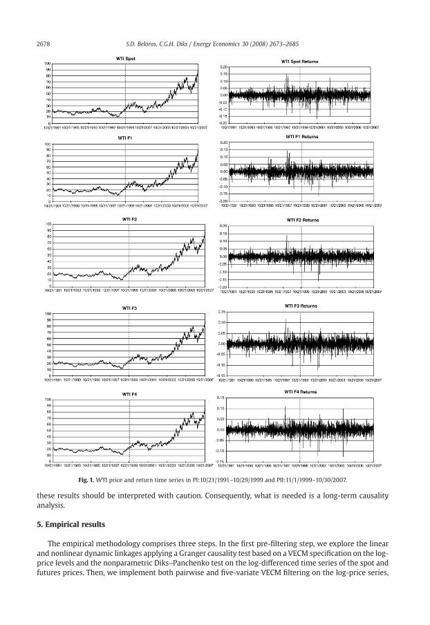
The data cover two equally sampled periods, namely PI which spans October 21,1991 to October 29,1999(2061 observations) and PII November 1,1999 toOctober 30, 2007 (2061 observations). The segmentation ofthe sample corresponds roughly to the reduction in OPEC spare capacity (defined as the difference betweensustainable capacity and current OPEC crude oil production) and to the increase in the United States'gasoline consumption and imports, both of which occurred after 1999. The effect of these events on pricedynamics is evident and it can be summarized in the accelerated rise of the average level of oil prices and inthe increased volatility (Regnier, 2007). Additionally, in PII markets witnessed more occasional spikes incrude prices. Fig.1 displays the spot and future price and returns time series. The following notation is used:“WTI Spot” is the spot price and “WTI F1”, “WTI F2”, “WTI F3” and “WTI F4” are the futures prices formaturities of one, two, three and four months respectively. Descriptive statistics for WTI spot and futureslog-daily returns are reported in Table 1. Specifically, the returns are defined as rt=ln(Pt)− ln(Pt−1), where Ptis the closing price on day t. The differences between the two periods are quite evident in Table 1 where asignificant increase in variance can be observed as well as a higher dispersion of the returns distributionin Period II reflected in the lower kurtosis. Additionally, Period II witnessed many occasional negativespikes as it can be also inferred from the skewness. The results from testing nonstationarity are presented inTable 2.
Specifically, Table 2 reports the Augmented Dickey–Fuller (ADF) test for the logarithmic levels and log-daily returns. The lag lengths which are consistently zero in all cases were selected using the SchwartzInformation Criterion (SIC). All the variables appear to be nonstationary in log-levels and stationary in log-returns based on the reported p-values. Table 1 also reports the correlation matrix at lag 0(contemporaneous correlation) for both periods. Significant sample cross-correlations are noted for spotand futures returns indicating a high interrelationship between the two markets. However, since linearcorrelations cannot be expected to fully capture the long-term dynamic linkages in a reliable way,
Fig. 1. WTI price and return time series in PI:10/21/1991–10/29/1999 and PII:11/1/1999–10/30/2007.
these results should be interpreted with caution. Consequently, what is needed is a long-term causalityanalysis.
5. Empirical results
The empirical methodology comprises three steps. In the first pre-filtering step, we explore the linearand nonlinear dynamic linkages applying a Granger causality test based on a VECM specification on the log-price levels and the nonparametric Diks–Panchenko test on the log-differenced time series of the spot andfutures prices. Then, we implement both pairwise and five-variate VECM filtering on the log-price series,
2679S.D. Bekiros, C.G.H. Diks / Energy Economics 30 (2008) 2673–2685
and the residuals are examined by the Diks-Panchenko test. Finally, we investigate the hypothesis ofnonlinear Granger non-causality after controlling for conditional heteroskedasticity using a GARCH-BEKKfilter, again in a bivariate and a five-variate representation. Additionally, in the last two steps we con-sistently apply a linear Granger causality test on the “whitened” residuals via a VAR specification (i.e., nocointegration detected on the residuals) in order to investigate whether any remaining causality is strictlynonlinear in nature or not.
The results are reported in the corresponding panels of Tables 3 and 4. In order to overcome thedifficulty of presenting large tables with numbers we use the following simplifying notation: “⁎⁎”
All variables are in logarithms and reported numbers for the augmented Dickey–Fuller test are p-values. The number of lags inparenthesis is selected using the SIC. (⁎⁎) denotes p-value corresponding to 99% confidence level.PI: 10/21/1991–10/29/1999; PII: 11/1/1999–10/30/2007.
Table 3Causality results (Pairwise)
Variables Panel A: linear Granger causality Panel B: non-linear causality
X Y Raw data VECM residuals GARCH-BEKKresiduals
Raw data VECM residuals GARCH-BEKKresiduals
X→Y Y→X X→Y Y→X X→Y Y→X X→Y Y→X X→Y Y→X X→Y Y→X
PI PII PI PII PI PII PI PII PI PII PI PII PI PII PI PII PI PII PI PII PI PII PI PII
(⁎),(⁎⁎) Denotes p-value statistical significance at 5% and 1% level. X→Y: rX does not Granger Cause r Y. PI: 10/21/1991–10/29/1999; PII:11/1/1999–10/30/2007.Panel A: Linear Granger Causality.All data (log-levels) were found to be cointegrated and the lag lengths of VECM specification are set using the Wald exclusioncriterion. The number of lags (in parenthesis) identified in period PI are: WTI Spot — WTI F1 (3), WTI Spot— WTI F2 (7), WTI Spot —WTI F3 (3), WTI Spot — WTI F4 (3) and in period PII: WTI Spot — WTI F1 (3), WTI Spot — WTI F2 (6), WTI Spot — WTI F3 (6), WTISpot—WTI F4 (4). In period PI for all pairs the Johansen test identified two (2) cointegrating vectors using the trace statistic and in PIIone (1) cointegrating vector again for all pairs. The causality on the VECM residuals was investigated with a VAR specification (the nullof no cointegration was not rejected) and the lags were determined using the Schwartz Information Criterion (SIC). The number oflags identified for all variables in all periods is one (1). The second moment filtering was performed with a GARCH-BEKK (1,1) model.Panel B: Non-Linear Causality.The number of lags used for the nonlinear causality test are ℓX=ℓY=1. The data used are log-returns. Since the log-levels were foundto be cointegrated (Panel A) the nonlinear causality was investigated on the VECM residuals. The number of lags (Wald exclusioncriterion) and the number of cointegrating vectors (Johansen trace statistic test) identified for the VECM specification are reported inPanel A. The second moment filtering was performed with a GARCH-BEKK (1,1) model.
indicating that the corresponding p-value of a particular causality test is smaller than 1% and “⁎” that thecorresponding p-value of a test is in the range 1–5%; Directional causalities will be denoted by thefunctional representation →.
Table 4Causality results (five-variate)
Variables Panel A: linear Granger causality Panel B: non-linear causality
X Y Raw data VECM residuals GARCH-BEKKresiduals
Raw data VECM residuals GARCH-BEKKresiduals
X→Y Y→X X→Y Y→X X→Y Y→X X→Y Y→X X→Y Y→X X→Y Y→X
PI PII PI PII PI PII PI PII PI PII PI PII PI PII PI PII PI PII PI PII PI PII PI PII
WTI Spot WTI F1 ⁎ ⁎⁎ ⁎⁎ ⁎⁎ ⁎⁎ ⁎⁎ ⁎ ⁎⁎ ⁎ ⁎ ⁎ ⁎
WTI Spot WTI F2 ⁎⁎ ⁎⁎ ⁎⁎ ⁎⁎ ⁎⁎ ⁎⁎ ⁎
WTI Spot WTI F3 ⁎⁎ ⁎⁎ ⁎⁎ ⁎ ⁎⁎ ⁎⁎ ⁎⁎ ⁎⁎ ⁎⁎
WTI Spot WTI F4 ⁎⁎ ⁎⁎ ⁎⁎ ⁎⁎ ⁎⁎ ⁎⁎ ⁎⁎ ⁎⁎ ⁎
(⁎),(⁎⁎) Denotes p-value statistical significance at 5% and 1% level. X→Y: rX does not Granger Cause r Y. PI: 10/21/1991–10/29/1999; PII:11/1/1999–10/30/2007.Panel A: Linear Granger Causality.The 5x5 system of the data (log-levels) was found to be cointegrated and the lag length of the VECM specification was set using theWald exclusion criterion. The number of lags identified in PI is eleven (11) and in PII is nine (9). In period PI the Johansen test identifiedfive (5) cointegrating vectors using the trace statistic and in PII three (3). The causality on the VECM residuals was investigated with aVAR specification (the null of no cointegration was not rejected) and the lags were determined using the Schwartz InformationCriterion (SIC). The number of lags identified for all variables in all periods is one (1). The second moment filtering was performedwith a GARCH-BEKK (1,1) model.Panel B: Non-Linear Causality.The number of lags used for the nonlinear causality test are ℓX=ℓY=1. The data used are log-returns. Since the 5-variate system oflog-levels was found to be cointegrated (Panel A) the nonlinear causality was investigated on the VECM residuals. The number of lags(Wald exclusion criterion) and the number of cointegrating vectors (Johansen trace statistic test) identified for the VECM specificationare reported in Panel A. The second moment filtering was performed with a GARCH-BEKK (1,1) model.
2681S.D. Bekiros, C.G.H. Diks / Energy Economics 30 (2008) 2673–2685
5.1. Causality testing on raw data
The linear Granger causality test is usually constructed in the context of a reduced-form vectorautoregression (VAR). Let Yt the vector of endogenous variables and ℓ number of lags. Then the VAR(ℓ)model is given as follows:
Yt ¼XSs¼1
AsYt�s þ et ð7Þ
Yt=[Y1t,…,Yℓt] the ℓ×1 vector of endogenous variables, As the ℓ×ℓparameter matrices and εt the� � � �
whereresidual vector, for which E etð Þ ¼ 0; E ete
0s ¼ Se t ¼ s
0 tps . Specifically, in case of two time series {Xt} and{Yt}~ I(1) (for example log-prices) the bivariate VAR model is given by:
DXt ¼ A Sð ÞDXt þ B Sð ÞDY þ eDX;tDYt ¼ C Sð ÞDXt þ D Sð ÞDY þ eDY ;t
t ¼ 1;2; N ;N ð8Þ
ΔXt, ΔYt the first differences of {Xt}, {Yt} and A(ℓ), B(ℓ), C(ℓ), D(ℓ) are all polynomials in the lag
whereoperator with all roots outside the unit circle. The error terms are separate i.i.d. processes with zero meanand constant variance. The test whether Y strictly Granger causes X is simply a test of the joint restrictionthat all the coefficients of the lag polynomial B(ℓ) are zero, whilst similarly, a test of whether X strictlyGranger causes Y is a test regarding C(ℓ). In each case, the null hypothesis of no Granger causality isrejected if the exclusion restriction is rejected. If both joint tests for significance show that B(ℓ) and C(ℓ)are different from zero, the series are bi-causally related. However, in order to explore effects of possiblecointegration, a VAR in error correction form (Vector Error Correction Model — VECM) is estimated usingthe methodology developed by Engle and Granger (1987) and expanded by Johansen (1988) and Johansenand Juselius (1990). The bi-variate VECM model has the following form:
DXt ¼ �p1 1 �k½ � � Yt�1Xt�1
�� þ A Sð ÞDXt þ B Sð ÞDYt þ eDX;t
DYt ¼ �p2 1 �k½ � � Yt�1Xt�1
�� þ C Sð ÞDXt þ D Sð ÞDYt þ eDY;t
t ¼ 1;2; :::;N ð9Þ
[1−λ] the cointegration vector and λ the cointegration coefficient. Thus, in case of cointegrated time
whereseries, linear Granger causality should be investigated via the VECM specification.
For the pairwise implementation the linear causality testing was carried out using the Granger's testbased on a VECM model of the log-prices because all series were found to be cointegrated. The lag lengthsof the VECM specification were set using the Wald exclusion criterion and for each pair in PI are(in parenthesis): WTI Spot — WTI F1 (3), WTI Spot — WTI F2 (7), WTI Spot — WTI F3 (3) and WTI Spot —WTI F4 (3). Similarly, in period PII: WTI Spot— WTI F1 (3), WTI Spot — WTI F2 (6), WTI Spot— WTI F3 (6)and WTI Spot—WTI F4 (4). In addition, in PI for all pairs the Johansen test identified two (2) cointegratingvectors using the trace statistic and in PII one (1) cointegrating vector. In case of the five-variateimplementation cointegration was also detected and in particular in PI the Johansen test identified five (5)cointegrating vectors while in PII three (3). The number of lags for the 5x5 system in PI was eleven (11) andin PII nine (9).
For the Diks–Panchenko test, in what follows we discuss results for lags ℓX=ℓY=1. Moreover, the test wasapplied directly on log-returns. To implement the test, the constantC for the bandwidth εnwas set at 7.5,whichis close to the value 8.0 for ARCH processes suggested by Diks and Panchenko (2006). With the theoreticaloptimal rateβ=2/7 given by Diks and Panchenko (2006), this implies a bandwidth value of approximately onetimes the standard deviation of the time series for both PI and PII. Selecting bandwidth values smaller (larger)than one times the standard deviation resulted, in general, in larger (smaller) p-values.
The results presented in Tables 3 and 4 allow for the following remarks: In the pairwise implementationof the linear Granger tests (VECM), strong bi-directional Granger causality between spot and futures priceswas detected in both periods with small differences regarding the degree of statistical significance.An exception could be that WTI Spot and WTI F4 present only unidirectional linear relationship WTISpot→WTI F4. On the contrary, the linear causality for the five-variate implementation appears to be uni-
directional, mainly in themore volatile and trending period PII and from spot to futures prices regardless ofmaturity, providing evidence that spot tend to lead futures prices. This indicates that spot prices can beuseful in the prediction of futures prices under a 5×5 VECM formulation, i.e., accounting for thecontributions of all maturities in the causality detection. Further, there is a causal relationship in PI of WTISpot→WTI F1, WTI F3→WTI Spot and WTI F4→WTI Spot. The nonlinear causality test revealed a bi-directional nonlinear relationship in PI, whereas in PII only uni-directional causality was detected fromSpot to WTI F1, WTI F2 and WTI F3 returns, excluding WTI F4.
5.2. Causality testing on VECM-filtered residuals
The results from the previous step suggest that there are significant and persistent linear and nonlinearcausal linkages between the spot and futures prices. However, even though we found nonlinear causality,the Diks–Panchenko test should be reapplied to the filtered VECM-residuals to ensure that any causalityfound is strictly nonlinear in nature. The number of lags and the number of cointegrating vectors identifiedfor the VECM specificationwere reported in the previous section. Moreover, a linear Granger test is appliedto the filtered residuals to conclude on a remaining linear structure even after filtering. The causality on thefiltered residuals was investigated with a VAR specification (the null of no cointegration was not rejected)and the lags were determined using the Schwartz Information Criterion (SIC).
The pairwise implementation of the Granger tests after VECM filtering shows that the linear causalrelationships detected on the raw returns have now disappeared. In fact none of the previously mentionedcausalities appear or any other new ones have emerged after linear filtering. Similarly, no causal rela-tionship could be detected after five-variate filtering. The application of the nonlinear test on the VECMresiduals, both in the bivariate and five-variate implementation, points towards the preservation of the bi-directional causality reported in PI on the raw log-returns. In PII the nonlinear causal relationships WTISpot→WTI F2,WTI Spot→WTI F3 have vanished, whileWTI Spot→WTI F1 remains, albeit statistically lesssignificant. Interestingly, in the same period, a uni-directional causality from futures to spot returns hasnow emerged for all maturities.
The nature and source of the detected nonlinearities are different from that of the linear Grangercausality and may also imply a temporary, or long-term, causal relationship between the spot and futuresmarkets. For instance, excess volatility in PII might have induced nonlinear causality. The nature of thevolatility transmission mechanism can be investigated after controlling for conditional heteroskedasticityusing a GARCH-BEKK model, in a bi-variate and five-variate representation.
5.3. Causality testing on GARCH-BEKK filtered VECM-residuals
The use of the Diks–Panchenko test on filtered data with a multivariate GARCH model enables one todetermine whether the posited model is sufficient to describe the relationship among the series. If thestatistical evidence of nonlinear Granger causality lies in the conditional variances and covariances then itwould be strongly reduced when the appropriate multivariate GARCH model is fitted to the raw or linearlyfiltered data. However, failure to accept the no-causality null hypothesis may also constitute evidence thatthe selectedmultivariate GARCHmodel was incorrectly specified. This line of analysis is similar to the use ofthe univariate BDS test on raw data and on GARCH models (Brock et al., 1996; Brooks, 1996; Hsieh, 1989).Many GARCH models can be used for this purpose. In the present study the GARCH-BEKK model of Engleand Kroner (1995) is used. The BEKK (p,q) model is defined as:
Ht ¼ CVCþXqj¼1
AVjket�jeVt�jAjk þXpj¼1
GVjkHt�jGjk; et ¼ H1=2t vt ð10Þ
C, Ajk and Gjk are (N×N) matrices and C is upper triangular.Ht is the conditional covariancematrix of
where{εt} with εt|Φt−1~(0, Ht) and Φt−1 the information set at time t−1. The residuals are obtained by thewhiteningmatrix transformationH1/2εt. Gourieroux (1997) gives sufficient conditions for At and Gt in orderto guarantee that Ht is positive definite.
Tables 3 and 4 show results before and after GARCH-BEKK (1,1) filtering. The order parameters weredetermined for the time series in terms of the minimal SIC. The linear Granger causality interdependencies
2683S.D. Bekiros, C.G.H. Diks / Energy Economics 30 (2008) 2673–2685
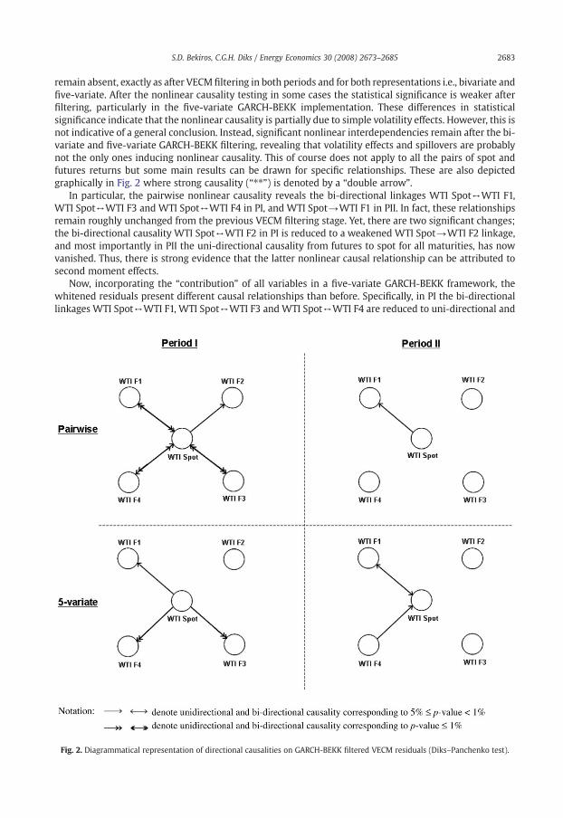
remain absent, exactly as after VECM filtering in both periods and for both representations i.e., bivariate andfive-variate. After the nonlinear causality testing in some cases the statistical significance is weaker afterfiltering, particularly in the five-variate GARCH-BEKK implementation. These differences in statisticalsignificance indicate that the nonlinear causality is partially due to simple volatility effects. However, this isnot indicative of a general conclusion. Instead, significant nonlinear interdependencies remain after the bi-variate and five-variate GARCH-BEKK filtering, revealing that volatility effects and spillovers are probablynot the only ones inducing nonlinear causality. This of course does not apply to all the pairs of spot andfutures returns but some main results can be drawn for specific relationships. These are also depictedgraphically in Fig. 2 where strong causality (“⁎⁎”) is denoted by a “double arrow”.
In particular, the pairwise nonlinear causality reveals the bi-directional linkages WTI Spot↔WTI F1,WTI Spot↔WTI F3 and WTI Spot↔WTI F4 in PI, and WTI Spot→WTI F1 in PII. In fact, these relationshipsremain roughly unchanged from the previous VECM filtering stage. Yet, there are two significant changes;the bi-directional causality WTI Spot↔WTI F2 in PI is reduced to a weakened WTI Spot→WTI F2 linkage,and most importantly in PII the uni-directional causality from futures to spot for all maturities, has nowvanished. Thus, there is strong evidence that the latter nonlinear causal relationship can be attributed tosecond moment effects.
Now, incorporating the “contribution” of all variables in a five-variate GARCH-BEKK framework, thewhitened residuals present different causal relationships than before. Specifically, in PI the bi-directionallinkages WTI Spot↔WTI F1, WTI Spot↔WTI F3 and WTI Spot↔WTI F4 are reduced to uni-directional and
Fig. 2. Diagrammatical representation of directional causalities on GARCH-BEKK filtered VECM residuals (Diks–Panchenko test).
the WTI Spot→WTI F2 has disappeared. It seems that the nonlinear causality from futures to spot returnswhich persisted even after the five-variate VECM filtering was induced by conditional heteroskedasticityand thus a five-variate and not a bi-variate GARCH-BEKK filtering of the VECM-residuals is better at“capturing” the volatility transmission mechanism. Instead, in PII the uni-directional linkages WTIF1→WTI Spot andWTI F4→WTI Spot were not entirely removed as in the bi-variate GARCH-BEKK filteringof the VECM-residuals. Eventually, in all results, third or higher-order causalitymay be a significant factor ofthe remaining interdependence.
6. Conclusions
In the present paper we investigated the existence of linear and nonlinear causal relationships betweenthe daily spot and futures prices for maturities of one, two, three and four months of West TexasIntermediate (WTI), which is the underlying commodity of New York Mercantile Exchange's (NYMEX) oilfutures contracts. The data covered two separate periods, namely PI: 10/21/1991–10/29/1999 and PII: 11/1/1999–10/30/2007, with the latter being significantly more turbulent. The study contributed to the literatureon the lead–lag relationships between the spot and futures markets in several ways. In particular, it wasshown that the pairwise VECMmodeling suggested a strong bi-directional Granger causality between spotand futures prices in both periods, whereas the five-variate implementation resulted in a uni-directionalcausal linkage from spot to futures prices only in PII. This empirical evidence appears to be in contrast to theresults of Silvapulle and Moosa (1999) on the futures to spot prices uni-directional relationship. Addi-tionally, whilst the linear causal relationships have disappeared after the cointegration filtering, nonlinearcausal linkages in some cases were revealed andmore importantly persisted even aftermultivariate GARCHfiltering during both periods. Interestingly, it was shown that the five-variate implementation of theGARCH-BEKK filtering, as opposed to the bi-variate, captured the volatility transmission mechanism moreeffectively and removed the nonlinear causality due to second moment spillover effects.
Moreover, the results imply that if nonlinear effects are accounted for, neither market leads or lags theother consistently, or in other words the pattern of leads and lags changes over time. Given that causalitycan vary from one direction to the other at any point in time, a finding of bi-directional causality over thesample period may be taken to imply a changing pattern of leads and lags over time, providing support tothe Kawaller et al. (1988) hypothesis. According to that hypothesis, market participants filter informationrelevant to their positions as new information arrives and, at any time point, spot may lead futures and viceversa. Hence it can be safely concluded that, although in theory the futures market play a bigger role in theprice discovery process, the spot market also plays an important role in this respect. The empirical evidenceof a causal linkage from spot to futures prices can be attributed to the sequence of actions taken from thethree market participants following a spot price change, as described in the Moosa model (1996). In that,arbitrageurs respond to the violation of the cost-of-carry condition and then speculators acting upon theexpected spot price will revise their expectation. In the same way, speculators who act upon the expectedfutures price will revise their expectation and react to the disparity between current and expected futuresprices. These conclusions, apart from offering a much better understanding of the dynamic linear andnonlinear relationships underlying the crude oil spot and futures markets, may have important im-plications for market efficiency. For instance, they may be useful in future research to quantify the processof market integration or may influence the greater predictability of these markets.
An interesting subject for future research is the nature and source of the nonlinear causal linkages. Aspresented, volatility effects may partly account for nonlinear causality. The GARCH-BEKK model partiallycaptured the nonlinearity in daily spot and future returns, but only in some cases. An explanation could bethat spot and futures returns may exhibit statistically significant higher-order moments. A similar resultwas reported by Scheinkman and LeBaron, (1989) for stock returns. Alternatively, parameterized asym-metric multivariate GARCHmodels could be employed in order to accommodate the asymmetric impact ofunconditional shocks on the conditional variances.
Acknowledgement
The authors acknowledge financial support from the Netherlands Organisation for Scientific Research(NWO) under the project: Information Flows in Financial Markets. The usual disclaimer applies.
2685S.D. Bekiros, C.G.H. Diks / Energy Economics 30 (2008) 2673–2685
References
Abhyankar, A., 1996. Does the stock index futures market tend to lead the cash? New evidence from the FT-SE 100 stock index futuresmarket. Working paper, vol. 96–01. Department of Accounting and Finance, University of Stirling.
Baek, E., Brock, W., 1992. A general test for non-linear Granger causality: bivariate model. Working paper, Iowa State University andUniversity of Wisconsin, Madison, WI.
Bopp, A.E., Sitzer, S., 1987. Are petroleum futures prices good predictors of cash value? The Journal of Futures Markets 7, 705–719.Brock, W.A., Dechert, W.D., Scheinkman, J.A., LeBaron, B., 1996. A test for independence based on the correlation dimension.
Econometric Reviews 15 (3), 197–235.Brooks, C., 1996. Testing for nonlinearities in daily pound exchange rates. Applied Financial Economics 6, 307–317.Chen, A.-S., Lin, J.W., 2004. Cointegration and detectable linear and nonlinear causality: analysis using the London Metal Exchange
lead contract. Applied Economics 36, 1157–1167.Choudhury, A.R., 1991. Futures market efficiency: Evidence from cointegration tests. The Journal of Futures Markets 11, 577–589.Cologni, A., Manera, M., 2008. Oil prices, inflation and interest rates in a structural cointegrated VAR model for the G-7 countries.
Energy Economics 30, 856–888.Crowder, W.J., Hamed, A., 1993. A cointegration test for oil futures market efficiency. Journal of Futures Markets 13, 933–941.Diks, C., Panchenko, V., 2005. A note on the Hiemstra–Jones test for Granger noncausality. Studies in Nonlinear Dynamics and
Econometrics 9 art. 4.Diks, C., Panchenko, V., 2006. A new statistic and practical guidelines for nonparametric Granger causality testing. Journal of Economic
Dynamics & Control 30, 1647–1669.Dwyer, G.P., Wallace, M.S., 1992. Cointegration and market efficiency. Journal of International Money and Finance 11, 318–327.Engle, R.F., Granger, C.W.J., 1987. Cointegration, and error correction: representation, estimation and testing. Econometrica 55,
251–276.Engle, R.F., Kroner, F.K., 1995. Multivariate simultaneous generalized ARCH. Econometric Theory 11, 122–150.Garbade, K.D., Silber, W.L., 1983. Price movement and price discovery in futures and cash markets. Review of Economics and Statistics
65, 289–297.Granger, C.W.J., 1969. Investigating causal relations by econometric models and cross-spectral methods. Econometrica 37, 424–438.Gourieroux, C., 1997. ARCH models and Financial applications. Springer Verlag.Hiemstra, C., Jones, J.D., 1994. Testing for linear and nonlinear Granger causality in the stock price–volume relation. Journal of Finance
49, 1639–1664.Houthakker, H.S., 1992. In: Newman, P., Milgate, M., Eatwell, J. (Eds.), Futures trading. The new Palgrave dictionary of money and
finance, vol. 2. Macmillan, London, pp. 211–213.Hsieh, D., 1989. Modeling heteroscedasticity in daily foreign exchange rates. Journal of Business and Economic Statistics 7, 307–317.Hull, J., 2000. Options, Futures and Other Derivatives. Prentice Hall, New York.Johansen, S., 1988. Statistical analysis of cointegration vectors. Journal of Economic and Dynamics and Control 12, 231–254.Johansen, S., Juselius, K., 1990. Maximum likelihood estimation and inference on cointegration with application to the demand for
money. Oxford Bulletin of Economics and Statistics 52, 169–209.Kawaller, I.G., Koch, P.D., Koch, T.W., 1988. The relationship between the S&P 500 index and the S&P 500 index futures prices. Federal
Reserve Bank of Atlanta Economic Review 73 (3), 2–10.Krehbiel, T., Adkins, L.C., 1993. Cointegration tests of the unbiased expectations hypothesis in metals markets. The Journal of Futures
Markets 13, 753–763.Moosa, I.A.,1996. In:McAleer,M., Miller, P., Leong, K. (Eds.), An econometricmodel of price determination in the crude oil futures markets.
Proceedings of the Econometric Society Australasian meeting, vol. 3. University of Western Australia, Perth, pp. 373–402.Moosa, I.A., Al-Loughani, N.E., 1995. The effectiveness of arbitrage and speculation in the crude oil futures market. The Journal of
Futures Markets 15, 167–186.Newberry, D.M., 1992. In: Newman, P., Milgate, M., Eatwell, J. (Eds.), Futures markets: Hedging and speculation. The new Palgrave
dictionary of money and finance, vol. 2. Macmillan, London, pp. 207–210.Oellermann, C.M., Brorsen, B.W., Farris, P.L., 1989. Price discovery for feeder cattle. The Journal of Futures Markets 9, 113–121.Regnier, E., 2007. Oil and energy price volatility. Energy Economics 29, 405–427.Sadorsky, P., 2000. The empirical relationship between energy futures prices and exchange rates. Energy Economics 22 (2), 253–266.Scheinkman, J., LeBaron, 1989. Nonlinear dynamics and stock returns. The Journal of Business 62 (3), 311–337.Schroeder, T.C., Goodwin, B.K., 1991. Price discovery and cointegration for live hogs. The Journal of Futures Markets 11, 685–696.Schwarz, T.V., Szakmary, A.C., 1994. Price discovery in petroleum markets: Arbitrage, cointegration, and the time interval of analysis.
The Journal of Futures Markets 14, 147–167.Serletis, A., Banack, D., 1990. Market efficiency and cointegration: an application to petroleum market. Review of Futures Markets 9,
372–385.Silvapulle, P., Moosa, I.A., 1999. The relationship between spot and futures prices: evidence from the cruide oil market. The Journal of