CONCORDIA UNIVERSITY Energy Optimization of a Cellular Network with QoS Guarantee by Arash Ansari Presented in Partial Fulfillment of the Requirements for the Degree of Master of Computer Science in the Department of Computer Science and Software Engineering Faculty of Engineering and Computer Science August 2017 c Arash Ansari, 2017
Transcript
CONCORDIA UNIVERSITY
Energy Optimization of
a Cellular Network
with QoS Guarantee
by
Arash Ansari
Presented in Partial Fulfillment of the Requirements
for the Degree of Master of Computer Science
in the
Department of Computer Science and Software Engineering
Global mobile data traffic was increased by up to 75% in 2016 and is expected to keep
growing at a Compound Annual Growth Rate (CAGR) of 42% by 2022. The number of
mobile devices and connections worldwide is expected to reach 11.6 billion by 2020, which
will be approximately 50% more than the world population in 2020 [1]. This includes
not only the 8.2 billion personal portable or mobile devices but also 3.2 billion M2M
(machine-to-machine) connections (e.g., Global Positioning System (GPS) in cars, goods
tracking systems in shipping and manufacturing sectors, medical applications keeping
patient records and health status). North America is experiencing the fastest growth of
mobile devices and connections with a 22% CAGR between 2015 and 2020 [2]. This is
an indication of the gigantic size of mobile communications industry.
This growing number of mobile devices leads to a continuous increase in cellular net-
works energy consumption. A typical cellular network consists of three main elements:
the core network (interface to fixed network), base stations and mobile terminals. At
present, most of the energy in mobile networks (up to 80%) is consumed by base stations
[4]. There is an increased number of installed base stations worldwide and, as a conse-
quence, there is a significant growth in the total energy consumed by mobile networks
[5, 6]. Currently, there are more than 4 billion base stations installed worldwide, each
consuming an energy equal to two average households.
1
Chapter 1 Introduction 2
Figure 1.1: Total number of global mobile devices (billion). (Statistics from Ericssonmobility report, 2017 [3]).
Figure 1.2: Global mobile data traffic (exabytes/month). (Statistics from Ericssonmobility report, 2017 [3]).
Base stations in cellular networks are often underutilized. While the load profile and
network traffic exhibit large variations between peak and off-peak values (with long
periods of low load), network operators plan their deployment with respect to peak
traffic usage [7, 8]. Operators are more concerned about the Quality of Service (QoS)
and data rates offered to the users and care less about the network energy consumption
[9]. Since the major base station power consumption is not load proportional, it is
difficult to achieve energy efficiency under low loads.
Chapter 1 Introduction 3
1.2 Sleep modes and energy optimization problem in cel-
lular networks
Sleep mode is considered as one of the most powerful approaches to minimize the energy
consumption of a cellular network [10, 11]. The proposition is to put weakly loaded base
stations into sleep mode or discontinuous transmission (DTX) mode during the off-peak
hours. In a sleep mode, a base station serves no user and consumes a minimum amount
of energy. In other words, base station capacity should be available only when and where
it is needed; it does not need to be available all the time [12].
However, switching off base stations results in increased interference as well as larger
distances between users and serving base stations [13]. Base stations sleeping algorithms
and strategies must consider the QoS of the users in the network. When a base station is
switched off, the neighbouring base stations must provide coverage over the region which
is no longer covered by the switched off base station. On the other hand, increasing
the energy of neighbouring base stations results in higher interference. To summarize,
interference, coverage, available channels and user assignment problems may conflict and
must be studied jointly to obtain an energy/performance trade off [14]. The ultimate
goal is to redirect sufficient power over an adequate number of channels so that mobile
operators can always guarantee the required QoS and data rate to the users.
1.3 Contribution of this thesis
In this work, an optimization model and its accurate solution is proposed to minimize the
power consumption of an LTE cellular network while guaranteeing a minimum data rate
for each mobile user. Taking interference into consideration, the proposed optimization
framework finds a solution for user - base station assignment problem in addition to
power and bandwidth allocation problems, assuming a proper call admission mechanism
has been put in place. The optimization model has been solved exactly for LTE networks
with up to 20 base stations and 450 users. For a given traffic, it outputs the best set of
active base stations to serve the users, the user assignment and the resource allocation,
Chapter 1 Introduction 4
while guaranteeing each user with the minimum required data rate. Moreover, applying
column generation method is investigated to solve larger instances of the problem.
In addition, a paper was published and presented at the 15th International Symposium
on Modeling and Optimization in Mobile, Ad Hoc, and Wireless Networks (WiOpt) in
March 2017 in Paris, France as a result of this thesis [15].
1.4 Thesis plan
The thesis is organized as follows. Chapter 2 reviews the problem background. Previous
related studies are reviewed in Chapter 3. Chapter 4 gives the detailed statement of
the problem, the newly proposed network optimization model and the solution process.
Moreover, the heuristic of Piunti et al. (2015) [12] is briefly recalled. In Chapter 5,
the use of column generation to improve the scalability of the model is investigated.
Numerical results, a comparison with the heuristic of [12], and sensitivity analysis of an
LTE network are presented in Chapter 6. Conclusions are drawn in the last Chapter.
Chapter 2
Background
In this Chapter, we review the background of the energy optimization problem in cellular
networks, terms, and networking concepts which are necessary to proceed with the rest
of this thesis. We start by an overview of cellular networks and their energy consumption
problem. Next, the sleep mode strategy to overcome this issue is introduced and the
associated challenges are discussed. Finally, the interference, data rate and quality of
service in a mobile network is reviewed.
2.1 Cellular networks
A cellular network is a wireless communication network that provides coverage over a
geographic area by dividing the land into small cells. Mobile User Equipment (UE)
in each cell is covered by a fixed location transceiver known as a Base Station (BS).
The most common example of a cellular network is the mobile network where a wide
geographic area (e.g., a city) is divided into smaller cells so that each mobile user can
receive or make a call through a base station. Dividing a huge area into small cells enables
us to overcome the problem of scarce frequency resources. As a result, we can re-use
the same frequency a few cells away from each base station. Thanks to the propagation
properties of radio waves, the same frequency can be safely reused by different base
stations without causing destructive interference if the proper distance is maintained
between the transmitters that are using the same waveform.
5
Chapter 2 Background 6
Normally, each UE receives transmitted signal from more than one base station. In
this situation the UE connects to the base station with the strongest received signal
power. This identifies the coverage region of each base station, which is referred to as a
cell. Since the received signal power decreases with the distance, it can be proved that
the strongest signal comes from the base station with the least geographical distance.
However, there exist cases (i.e., there are too many users close to a single base station)
where not all the users can be covered using this strategy.
2.2 Long term evolution (LTE)
Long Term Evolution (LTE), first deployed in 2009, represents the fourth generation
of cellular network technologies. It is a standard developed by 3rd Generation Part-
nership Project (3GPP) for high-speed communication of cellular networks. 3GPP is
a collaboration between major telecommunications standard development organizations
for different communication networks including cellular networks [16].
LTE employs advanced and efficient technologies to support high speed data connection
both in up-link and down-link. It can provide data rates up to 75 Mbps in the up-link
and 300 Mbps in the down-link [17]. Currently, less than 35% of mobile devices in the
world support LTE connection [3]. However, the number of LTE users is growing and it
is anticipated that LTE will become the dominant standard by the end of 2018 (Figure
2.1).
The communication channel in a cellular network (air) is shared among all users. In an
LTE system, several advanced technologies are deployed to allow users to communicate
over the shared channel. The main strategy is to divide resources (time and frequency)
into small slots and assign each user a separate slot. That is, at a specific time slot
and using a specific frequency, only a single user is communicating. Going over channel
access technologies in details is beyond the scope of this work 1.
1In the downlink, LTE uses orthogonal frequency division multiple access (OFDMA) and in theuplink, single carrier-frequency division multiple access (SC-FDMA). Refer to [18] to read more onchannel access methods in an LTE system.
Chapter 2 Background 7
Figure 2.1: Global LTE subscribers portion: it is anticipated that LTE will becomethe dominant standard by the end of 2018. (Statistics from Ericsson mobility report,
2017 [3]).
Figure 2.2: Physical resource block (PRB) and multiple channel access in an LTEsystem. A PRB cannot be shared among multiple users.
In an LTE system, the spectrum and the time is divided into smaller segments. Each
segment is called a Physical Resource Block (PRB). A PRB is a resource unit having
both time and frequency dimensions. This division of resources allows multiple users to
communicate over a shared channel. Each user will be assigned one or more PRBs for
communication, while a PRB cannot be shared among multiple users (Figure 2.2).
The number of available bandwidth blocks depends on the system bandwidth. In an LTE
system, the number of PRBs varies from 6 to 100 (depending on the channel bandwidth
Chapter 2 Background 8
which varies between 1.4-20 MHz) [18].
2.3 Infrastructure energy consumption
When the first generation of wireless mobile telecommunications technology (1G) was
introduced in 1981, the only purpose of a mobile network was to provide the possibility
of making phone calls for the users. However, this did not last long and 3G systems,
which were introduced in the early 2000, were designed to provide Internet data and
web-based applications in addition to the ability of making phone calls between users.
Today, the ability to access high speed Internet in a cellular network is more important
than making phone calls for many of the mobile users.
As the system tries to increase the data capacity, it becomes more difficult to find enough
spectrum. This problem can be overarmed by the cost of consuming more energy. In
2016, the number of global mobile devices and connections surpassed 8.0 billion, which
is more than the world population [1]. Providing coverage for this growing number of
mobile devices comes with the cost of enormously increasing energy consumption of
mobile networks.
There are two major sources of energy consumption in a wireless network: transmission
and computation. The transmitted energy depends on communication states, like QoS
requirements, transmission channel characteristics, etc. The computation energy is the
energy consumed by processing devices to perform signal processing and other computa-
tions. The energy consumed for computation depends on hardware, software, processing
algorithms, etc. For long-distance communications (e.g., macro cell communication) the
major energy consumer is transmission, while in short-distance communications (e.g.,
femtocell or WiFi) the major energy consumers are the processors.
In mobile networks, the energy is mostly consumed by base stations, both for commu-
nication and transmission (Figure 2.3). Since the number of available frequency blocks
at each base station is limited, mobile operators have to increase the number of base
stations to provide coverage for more users. If the number of users in an area is likely to
increase significantly during the day (e.g., in a shopping mall or a transportation hub)
Chapter 2 Background 9
Figure 2.3: Energy consumption in a cellular network: up to 80% is consumed by thebase stations
a usual macro cell is replaced with a number of smaller micro cells. Each microcell is
serving a smaller area, and therefore, more users can be covered in total. Dividing a
large cell into smaller cells does not stop at this level and in a similar way smaller cells,
namely picocells and femtocells, are also used for different use-cases.
2.4 Green cellular networks
Any increase in energy consumption comes with an increase in emission of pollutants and
greenhouse gasses (GHG - mainly carbon dioxide). Accumulation of GHG will speed up
global warming and climate changes which cause natural calamities like typhoons, floods
and changes in the sea levels. The information and communications technology (ICT)
industry is responsible for about 2% of GHG emissions. China, USA and Europe union
are major contributors causing almost 50% of of global GHG emissions [19]. Canada’s
share made up less than 2% of global GHG emissions [20]. U.S. government has recently
announced its withdrawal from “Paris climate accord”, which is an agreement within the
United Nations framework convention on climate change dealing with greenhouse gas
emissions mitigation. The U.S. government believes that this withdrawal would help
American businesses and workers. This shows that a solution to GHG accumulation
problem which does not cause big industries to lose their profit has a significant value.
Chapter 2 Background 10
A large number of studies in recent years have been focusing on green cellular networks.
The term green in wireless networks usually refers to a network which consumes less
energy and resource. Telecommunication industry has made a significant contribution
to reduce CO2 emissions in the recent years and one of the main objectives of the next
generation of mobile network standard (5G) is to make the network more efficient in
terms of power consumption and resource management.
2.5 Sleep modes
Current mobile networks are designed to satisfy the users needs during the peak hours
and are underutilized most of the time. In order to reduce energy consumption of the
network, a cell can be put into a sleep mode or discontinuous transmission (DTX) mode.
While in a sleep mode, the base station covers no user and consumes less energy. In the
deepest sleep mode the energy consumption is very close to zero. It is assumed that a
cell can go to a sleep mode very quickly, while going back to the active mode takes a
certain amount of time and energy based on the sleep mode level. The idea behind a
lighter sleep mode is to deactivate only selected parts of the cell hardware. This makes
the activation process faster [21]. In this thesis, we consider a single sleep mode.
Figures 2.4-2.6 illustrate the effect of base station sleeping on a cellular network. Figure
2.4 shows the UE distribution over a geographic area. This can be the center of a city
with a shopping center located at the north east area. While this area is very crowded
during the day, the network traffic can be very low during the night (i.e., when the
shopping center is closed). By covering the whole area by only a few base stations and
putting all other base stations into the sleep mode, energy consumption of network can
be significantly reduced.
2.6 Base station energy consumption model
While in sleep mode the base station consumes a constant power (depending on the
sleep level), its energy consumption depends on the load in the active mode. In general,
Chapter 2 Background 11
Figure 2.4: Sample user distribution during the peak hours
Figure 2.5: Sample user distribution during the off-peak hours
Figure 2.6: Turning off under-utilized base stations during the off-peak hours
Chapter 2 Background 12
energy consumption of a base station can be modelled as follows [22]:
P =
P0 + ∆p.Pout 0 < Pout ≤ Pmax
Psleep Pout = 0,
(2.1)
where P0 is the power consumption at the minimum non-zero output power, ∆p is the
slope of the load-dependent power consumption and Psleep is the power consumption of
the base station when in the sleep mode.
2.7 Interference
It was very easy to observe the interference in the old days when many AM radio stations
were trying to attract the attention of the audience. Radio audience could sometimes
hear an unwanted sound of another radio station in the background. This background
sound was being sent by another radio station far from them that was inadvertently
using the same frequency. Using limited resources extensively and simultaneously by
many different signal transmitters naturally leads to a conflict like this. In some cases,
the strength of the unwanted signal was so high that it would be possible to hear the
background sound clearly, if it was alone. [18]
Interference is the power of signal received from unwanted transmitters (usually far from
the user) which share the same bandwidth with the intended transmitter. Interference
disrupts the receiving signal. From the receiver’s point of view, interference modifies
and disrupts the received signal similar to a background noise. This is a serious issue
in mobile telecommunication as a huge number of base stations transmitting signal in
different locations relatively close to each other. There are several techniques to overcome
interference problem in a cellular network which is beyond the scope of this work. Our
focus is on the effect of base station transmission power on the network interference.
Chapter 2 Background 13
2.8 Quality of service, SINR and achievable data rate
Quality of service (QoS) refers to the overall performance of the network, which depends
on several characteristics, i.e., data rate, throughput, delay, etc. In this work, we focus
on the data rate received by each user, as this is the only characteristic which is highly
dependent on the base station transmission power. Using Shannon-Hartley theorem,
maximum achievable data rate (channel capacity) can be calculated as follows [23]:
C = W log2(1 +P
WN0) (2.2)
where C[b/s] is the channel capacity (achievable data-rate), W [Hz] is the bandwidth,
P [Watt] is the received power and N0[Watt/Hz] is noise power spectral density. Taking
interference into consideration, it is concluded that
C = W log2(1 +P
WN0 + I) (2.3)
where I[Watt] is the interference.
The term PWN0+I is refereed to as “Signal to Interference plus Noise Ratio”, or SINR.
In wireless communications SINR is the power of received signal divided by the sum of
background noise power and interference power. SINR is used to measure the quality of
the connection in wireless communications. A higher value of SINR in an indication of a
good quality channel with a clear transmitting signal and a week noise and interference.
Channel capacity is the theoretical upper bound for information transmission over a
communication channel. The actual data rate received by the user depends on other
factors as well, most importantly the coding of information. However, sending informa-
tion with transmission rates very close to the channel capacity is achievable in today’s
telecommunication.
Chapter 3
Literature Review
Several studies have already looked into the issues pertaining to coverage, throughput,
and energy trade-offs in cellular networks [11, 24]. Mobile networks are under utilized
most of the time and the main goal of these set of studies is to take advantage of
available network resources or improve energy efficiency of base stations to reduce the
energy consumption of mobile networks. For instance, assigning free bandwidth blocks to
the users at each base station can help reduce BS transmission power while maintaining
the same data-rate for users [25].
A first set of studies relate to single cells, and investigate the radio transmission processes
in order to reduce the energy consumption. Several parameters have been investigated,
and numerous studies exist, see, e.g., [25–27]. More recently, studies have investigated
beamforming and MIMO techniques [28, 29].
A second set of studies deal with multi-cell wireless networks, see, e.g., [30] for a rather
recent survey. Green scheduling and power control for both classic and heterogeneous
cellular networks are reviewed in [31]. For some recent studies related to 5G and MIMO
technology, see, e.g., [29].
In most of existing studies, network parameters are investigated separately, i.e., energy
consumption is optimized while the UE-BS assignment is known. In this thesis, we are
interested in exact methods for energy optimization in LTE networks, taking all network
parameters into consideration. While there have been many studies with decomposition
14
Chapter 3 Literature Review 15
techniques for throughput and energy optimization for a single BS [32–34], there exists
still no study with those techniques for LTE networks. This is explained by the fact
that the problem resembles some location problems [35], for which column generation
need to be combined with other techniques in order to be efficient.
Several works in wireless networks (e.g., see [33] and [34]) use column generation in en-
ergy optimization and power control problems to efficiently solve large problem instances.
In these works the idea of Independent Sets (ISets) is combined with column genera-
tion to deal with SINR constraint and guarantee a minimum QoS for the users. The
concept of transmission configurations (or independent sets, ISets for short) is defined
as a set of links that can transmit simultaneously without violating SINR constraint.
From an ISet, any combination of transmission configurations can be selected simulta-
neously without frustrating SINR constraint. The column generation model consists of
a master problem and a pricing problem: the master problem chooses one ISet for each
time frame and decides on selecting the best set of transmission configurations from the
selected ISet. Since master problem chooses the configurations from an ISet, it does not
need to worry about SINR constraint, as it is taken care by the pricing problem. The
pricing problem generates a new ISet at each iteration. It plays the role of generator of
transmission configurations such that, if added to the master problem, it improves the
solution of its linear relaxation. In order to apply the idea of ISets to a cellular network
problem, we need to consider possible transmission configurations instead of network
links. A transmission configuration is a set of users assigned to a base station together
with their transmission parameters. Then each ISet will be a set of transmission config-
urations that, if selected simultaneously, do not violate the SINR constraint. Therefore,
the master problem can select any subset of transmission configurations from an ISet to
cover all the users without being worried about the SINR constraint. However, unlike
the total number of links in a wireless mesh network, which is linear to the number of
nodes, the number of configurations in a cellular network is exponential to the number
of users. Because of the exponential number of possible user assignments, the ISet gen-
erator (pricing problem) becomes another large scale problem and this decomposition
does lead to a more efficient solution.
In this thesis, our focus is on the sleep mode, one of the classical mechanisms for energy
Chapter 3 Literature Review 16
efficiency. Previous studies for LTE networks include the work of Zhu et al. (2014) [36],
where a user association scheme based on cell sleeping has been proposed to reduce the
energy consumption under a simplifying strategy of equal bandwidth scheduling.
In [12], Piunti et al. (2015) proposed an iterative heuristic method for the cellular
network configuration with QoS guarantee. The proposed solution determines the user
association, bandwidth allocation, identification of active base stations and their trans-
mission power. The iterative method is based on a Mixed Integer Quadratic Program-
ming (MIQP) model that decides on BS-UE assignment together with the base stations
activity. User bandwidth, and the transmit power of each active base station are then
determined using different algorithms. The algorithm iterates until all the users are sat-
isfied with QoS requirements (see Section 4.3 for more details). However, this iterative
solution does not necessarily provide an optimum solution, mainly for two reasons: first
the QoS constraints are omitted from the MIQP model, and second, resources allocation
is done in a second phase and MIQP does not have the flexibility to decide on resource
allocation problems. The accuracy of the results provided by this solution decreases as
the size and traffic of the network growth and the network interference increases, see
Section 6.2.
In this thesis, we propose a model that minimizes the power consumption while taking
the interference constraints accurately into consideration using a SINR modelling. The
output of the model consists of the BS-UE assignment, the value of the transmission
power of each base station, the selection of the base stations to be put in sleep mode and
the bandwidth assigned to each user. This is the first work in the literature that finds
the optimal user-base station assignment and resource allocation, while guaranteeing to
satisfy each user with a minimum data rate in an LTE network.
Chapter 4
A First Model and its Solution
In this chapter, we define a mathematical model for the problem of energy optimization
in an LTE network. The heuristic solution of Piunti et al. (2015) [12] is reviewed after.
Then an exact solution is proposed to solve the proposed optimization model.
4.1 Statement of the EOCN problem
For a given LTE network, which is a given distribution of users and base stations over a
geographical area, the EOCN problem aims at minimizing the total energy consumption
of the network. The goal is to provide network coverage for all users but use only the
minimum energy required by network infrastructures.
We have three main resources in an LTE system: energy, time and spectrum. Energy is
modeled directly into the problem. Time and spectrum are modeled using PRB concept
which has both dimensions (as described in Section 2.2).
The EOCN problem decides on:
• The set of active base stations. Any base station which is not active will be put
on the sleep mode.
• BS-US association: assigning each user to an active base station.
17
Chapter 4 A First Model and its Solution 18
• Resource allocation
– Power assignment: determining the power transmitted to each user from its
serving base station.
– Physical resource (PRB) allocation: giving each mobile user a specific number
of physical resource blocks to receive data from the base station.
In the solution output by the model, all users must be covered by a base station and
satisfied with the minimum required data-rate. Moreover, allocated resources at each
base station cannot exceed the maximum available limit.
4.2 EOCN optimization model
We define a new mathematical model for the EOCN problem.
Parameters
We denote by B the set of base stations, indexed by b, and U the set of users, indexed
by u, assuming their locations to be distributed over a given area. Following are the
sets of variables and constants used in the optimization model.
Constants
• σbu ∈ R+: channel gain between base station b and user u. It mainly depends on
the b - u distance and determines the reduction of signal strength during transmis-
sion over channel. The power received by the user is equal to the power transmitted
by the base station multiplied by the channel gain between user and base station.
• N0[dBm/Hz]: noise power spectral density. This is the noise power per unit of
bandwidth.
• W [Hz]: total available bandwidth at each base station.
• Pmax[W ]: base station transmission power limit.
Chapter 4 A First Model and its Solution 19
• ru[bit/s]: minimum required data rate by each user u.
• pmin[W ]: user sensitivity. It is the minimum signal power each user equipment
needs to receive in order to be able to operate.
• Nprb: number of available PRBs at each base station. The total available PRBs
at each base station is divided to Nprb equal resource blocks.
• P0[W ]: base station power consumption at the minimum non-zero output power
• Psleep[W ]: power consumption of the base station when in the sleep mode
• ∆p: base station slope of the load-dependent power consumption
Decision variables
Following are the EOCN problem decision variables.
• abu ∈ {0, 1}: expresses the coverage association between base stations and users.
abu = 1 if the user u is assigned to base station b and abu = 0 otherwise.
• wbu and pbu are resource allocation variables:
– wbu ∈ Z+: number of bandwidth blocks (PRBs) allocated to user u by base
station b.
– pbu[W ] ∈ R+: power transmitted to u by base station b.
• Ib ∈ {0, 1}: activity binary variable for each base station. Ib = 1 if base station b
is active and Ib = 0 if b is in sleep mode.
Achievable data rate
One of the most important requirements the optimization model needs to satisfy is the
data rate constraint. Using (2.3) data rate received by each user can be calculated using
the following.
Chapter 4 A First Model and its Solution 20
C = W log2(1 +P
WN0 + I). (4.1)
We assume that the coding is efficient and the received rate is very close to the channel
capacity. This is a reasonable assumption in today’s mobile communication systems.
Using our notation, we can rewrite the channel capacity formula to find the user data
rate as the following.
ru =∑b∈B
abu wbu log2(1 + sinrbu),
where ru is the received data rate. SINR can be calculated using:
sinrbu =pbu σbu abu
wbuW
(∑b′∈B
Pb′Ib′σb′u(1− ab′u) +WN0
) (4.2)
where Pb =∑
u∈U pbu is the total power being transmitted by b.
Objective function
The objective function is written as follows:
min∑b∈B
(∆p.Pb + P0)Ib + Psleep(1− Ib). (4.3)
The goal is to minimize the global power consumption of the network. ∆p, P0 and Psleep
are base station power consumption parameters explained in Section 2.6. Pb, which is
the total transmission power of base station b (the sum of pbu) is defined to simplify the
notation.
Constraints can be expressed as follows:
Chapter 4 A First Model and its Solution 21
∑b∈B
abu = 1 u ∈ U (4.4)
∑b∈B
abuwbu log(1 + sinrbu) ≥ ru u ∈ U (4.5)
abu ≤pbuσbupminu
u ∈ U, b ∈ B (4.6)∑u∈U
pbu ≤ Pmax b ∈ B (4.7)
∑u∈U
abuwbu ≤ Nprb b ∈ B (4.8)
ε∑u∈U
abu ≤ Ib ≤∑u∈U
abu b ∈ B (4.9)
pbu ≥ 0, abu ∈ {0, 1}, wbu ∈ {1..Nbb} u ∈ U, b ∈ B (4.10)
Ib ∈ {0, 1} b ∈ B. (4.11)
All users must be covered and satisfied. Constraint (4.4) forces each user to be assigned
to one, and exactly one, base station. Constraint (4.5) is the bit-rate constraint: it
guarantees that each user is satisfied with its minimum required data rate. Note that
the minimum required data rate, ru, depends on each user, so that different users can be
provided with different data rates. Constraint (4.6) provides each user with a minimum
power, which should be greater than or equal to the user sensitivity. Constraint (4.7) is
the upper bound constraint for the transmission power of each base station. Constraint
(4.8) enforces a limitation on the maximum number of bandwidth blocks each base
station can provide. Constraint (4.9) determines the activity of the base stations: each
base station is active if it is serving at least one user. If no user is assigned to a base
station, it will be in sleep mode. Note that ε has to be small enough to limit the value
of ε∑
u∈U abu to a value always smaller than 1. This constraint forces the activity of
base station b if the value of∑
u∈U abu is not zero.
Chapter 4 A First Model and its Solution 22
4.3 Heuristic solution of Piunti et al. (2015)
In this section, we briefly recall the model and the MinPowerQos algorithm proposed by
Piunti et al. [12]. Therein, the authors propose a heuristic to solve the EOCN problem.
An iterative algorithm is used to deal with the non-linear bitrate constraint and to find
a solution to the EOCN problem, see [12] for more details. We will compare our exact
solution with the heuristic of [12] in Section 6.2.
In the solution of Piunti et al., a Mixed Integer Quadratic Program (MIQP) is defined
initially which is a simplified version of the EOCN model. The bandwidth assignment
and bit rate constraints from the EOCN optimization model are removed, i.e., constraints
(4.5) and (4.10) of EOCN model are omitted and constraints (4.8) are replaced by the
following ones: ∑u∈U
abu ≤ Nprb b ∈ B. (4.12)
This MIQP decides on BS-UE assignment only. Since the MIQP does not include the
non-linear constraint, i.e., constraint (4.5), it can be solved using an MIQP solver. The
provided solution determines the BS-UE association.
The bandwidth allocation and power assignment is not taken care by the MIQP model.
Therefore, it must be done in a second step. Several heuristics are suggested in [12]
for the bandwidth assignment. For example, the equal bandwidth assignment can be
used: it divides the available bandwidth blocks at each base station equally among the
assigned users. The next step is to solve the power allocation problem. Given a BS-UE
association and a bandwidth assignment, the power control algorithm suggested in [12]
provides the optimum BS transmission power. After applying power control to determine
the transmitting power, the received users’ data rate is calculated. For any user who is
not satisfied with the minimum data rate, its minimum required power is increased and
the MIQP is solved again. The algorithm iterates until all users are satisfied or there is
no feasible solution to the MIQP.
Note that MinPowerQos does not necessarily provide an optimal solution. User-base
station assignment and resource allocation are done in different steps and the assignment
Chapter 4 A First Model and its Solution 23
Figure 4.1: MinPowerQos heuristic of Piunti et al., 2015
while not all the users are satisfied doSolve MIQP and get a UE-BS association;Do the bandwidth and power allocation based on the UE-BS association;forall users do
Calculate receiving data rate;if the user is not satisfied then
increase the minimum power required by the not satisfied user, Pminu ;end
end
endReturn UE-BS association, power and bandwidth allocated to each user.
Algorithm 1: MinPowerQos huristic
Chapter 4 A First Model and its Solution 24
step does not take the bandwidth limitations, interference and bit-rate constraint into
consideration. Moreover, finding a feasible solution by the MinPowerQos huristic is not
guaranteed and the algorithm may fail to find a feasible solution (as the MIQP can
become infeasible after a few iterations). It can be seen (Section 6.2) that the gap
between the solution provided by the exact solution of EOCN model (see Section 4.4)
and the solution of this heuristic iterative process is small when the network load is low.
However, the gap increases as the network load and interference increases.
4.4 Exact solution of the EOCN problem
The bit-rate constraint (4.5) of the EOCN optimization model described in Section 4.2
is logarithmic and therefore is not linear. In order to deal with non-linearity of (4.5)
and solve the EOCN model, an exact linearization is proposed in this section.
In order to perform the linearization, we define a set of constants T r,w: for each data
rate r and bandwidth w, T r,w is the minimum SINR required for a user who is assigned
bandwidth w, and who requires data rate r.
Value of T r,w is given by the following formula:
T r,w = 2rw − 1.
Following is the proof. For each user, if the received sinr is greater than T r,w:
sinrbu ≥ T r,w = 2rw − 1
=⇒ w log2(sinrbu + 1) ≥ r
=⇒ ru ≥ r,
which shows that the bit-rate received by the user is greater than the required rate, r.
A new 0− 1 variable xwub is defined in order to select the right threshold for each user:
xwbu = 1 if user u is assigned the bandwidth w by base station b, 0 otherwise.
Chapter 4 A First Model and its Solution 25
Using variable xwub and constant T r,w, constraints (4.5) can be equivalently rewritten:
∑b∈B
abusinrbu ≥∑b∈B
∑w∈W
xwbuTr,w u ∈ U. (4.13)
For each user, the left-hand side of (4.13) is the sinr that the user receives and the
right-hand side is the minimum required sinr threshold.
Combining (4.2) with (4.13), and after performing some algebraic manipulations (manip-
ulations can be found in the Appendix), constraint (4.13) can be equivalently rewritten:
∑b∈B
∑w∈W
xwbuσbupbuW
T r,w− Pbσbu(1− abu) ≥WN0 u ∈ U, (4.14)
where Pb =∑u∈U
pbu is the total power that base station b consumes.
The new variable xwub needs to also satisfy the next two set of constraints:
∑w∈W
xwbu ≤ 1 u ∈ U, b ∈ B (4.15)
∑u∈U
∑w∈W
xwbu × w ≤W b ∈ B, (4.16)
where constraints (4.15) force each user to be assigned at most one specific number
of bandwidth blocks only, and constraints (4.16) guarantee that the total number of
assigned bandwidth blocks at each base station does not exceed the number of available
bandwidth blocks.
In other words, the logarithmic constraint (4.5) of the optimization model (4.4)-(4.11)
is replaced by the above linear constraints (4.14), (4.15) and (4.16). Note that the
proposed linearization is exact and does not alter the model constraints and limitations.
The solution of the resulting model is therefore exact and the algorithm will be referred
to as OptPowQoS in the sequel.
Chapter 4 A First Model and its Solution 26
4.5 Concluding remarks
In this section, we defined an optimization model to minimize energy consumption of
an LTE network. An exact solution is then proposed by linearizing the EOCN model.
Solution obtained by solving the EOCN model includes network energy consumption,
user base station assignment and resource allocation.
Chapter 5
A Column Generation Approach
5.1 Introduction
Column generation is a powerful tool for solving linear programs with a huge number
of variables [37, 38]. In this chapter, we investigate on using column generation to
overcome the scalability problem of the OptPowerQos solution suggested in Chapter 4.
In this chapter, the EOCN problem is reformulated and a column generation solution is
investigated to solve the EOCN problem.
We first review a related problem in operations research. The configuration concept
is defined after, which is necessary to reformulate the EOCN problem. Then a new
formulation of the EOCN problem is proposed and its solution using column generation
technique is presented.
5.2 Capacitated p-median: a related problem
Given a set of potential locations for a set of facility centers and a set of demand points
that must be serviced, the Capacitated p-Median Problem (CPMP) aims at locating p
facilities at potential locations to minimize the sum of the distances from each demand
point to its assigned facility center. In the capacitated p-median problem, each facility
location has a limited capacity to service the demands.
27
Chapter 5 A Column Generation Approach 28
The p-median problem is a well-known and well-investigated problem in operations re-
search. Several heuristics and exact solutions have been proposed in the literature to
solve the CPMP. Lorena and Senne (2003) [35] suggested a column generation approach
to the capacitated p-median problem. The authors show that Lagrangean/surrogate re-
laxation can accelerate the column generation process by generating new productive set
of columns. In [35], the authors identify Lagrangean/surrogate relaxation directly from
the master problem dual. It is shown that the Lagrangean/surrogate relaxation is able
to identify very good lower bounds and contributes with new columns that accelerate
the column generation process. Please refer to [35] for more details.
The EOCN problem can be compared with the CPMP as each base station can be
mapped to a facility center and each user can be mapped to a demand point. Although
EOCN is more constrained, both problems seek to locate facility centers (base stations)
close to the users. The major difference between the two problems is the complicated
data rate constraint (4.5) of EOCN problem which depends on all other base stations
and highly limits the feasibility area of the problem. Moreover, the CPMP objective
is to minimize the sum of the distances between demand points and facility centers,
while in EOCN problem the objective is to minimize the total cost associated with base
stations. Despite the differences, CPMP solution ideas can be useful to find a solution
to the EOCN problem.
In this chapter, we investigate on solving EOCN problem using the basic application of
column generation. Improving the quality of generated columns by applying Lagrangean
relaxation is beyond the scope of this thesis.
5.3 Configuration concept
In this section we define the concept of transmission configuration, which is needed to
reformulate the EOCN problem. For a given base station b, a transmission configuration,
denoted by γ, is a potential set of UEs assigned to b, together with their transmission
Chapter 5 A Column Generation Approach 29
parameters. Let Γ denote the overall set of configurations:
Γ =⋃b∈B
Γb,
where Γb denotes the set of configurations associated with b.
Each configuration γ is associated with a base station b, and is characterized by:
• aγu ∈ {0, 1} with aγu = 1 if u is assigned to b, and aγu = 0 otherwise.
• wγu = bandwidth assigned to u by b.
• pγu = power transmitted to u from b.
5.4 Objective
In this section, we define a new mathematical model, for the EOCN problem. The
EOCN CG ILP problem seeks to select a set of configurations consuming the minimum
total energy so that the selected configurations provide all the users with network cover-
age having all constraints satisfied. We define a decision variable zγ = 1 if configuration
γ is selected (0 otherwise). At most 1 configuration will be selected from each base
station, i.e., from each set Γb. If no configuration is selected from Γb, then b will be put
to sleep mode.
Each configuration γ consumes the total power Pγ and each BS in sleep mode consumes
Psleep energy amount.
The objective of EOCN CG ILP optimization model can be written as follows.
min∑γ∈Γ
Pγzγ +∑b∈B
Psleep(1−∑γ∈Γb
zγ) (5.1)
where:
Pγ = ∆p
∑u∈U
pγu + P0
Chapter 5 A Column Generation Approach 30
is the total power consumed by configuration γ.
Constraints:
∑γ∈Γ
aγu zγ = 1 u ∈ U (5.2)
∑γ∈Γb
zγ ≤ 1 b ∈ B (5.3)
∑γ∈Γ
aγuwγu log(1 + sinrγu)zγ ≥ ru u ∈ U (5.4)
zγ ∈ {0, 1} γ ∈ Γ. (5.5)
Constraints (5.2) guarantee that each user will be served by exactly one base station.
With (5.3), at most one configuration will be assigned to a base station and constraints
(5.4) guarantee the minimum bit-rate constraints for each user.
The set of all possible transmission configurations, Γ, grows exponentially with num-
ber of users. Therefore, the column generation model, EOCN CG ILP, is a large-scale
model containing an exponential number of variables, zγ . It is evident that complete
enumeration of all these variables is not an option. We will explain in Section 5.6 how
to solve this large scale model using an implicit enumeration of the variables.
5.5 Bit-rate constraint
Using the configuration notation, SINR calculation formula (5.4) can be re-written as:
sinrγu =Wσbu
pγuwγu∑
γ′∈Γ
P γσb′u(1− aγ′u )zγ′ +WN0
. (5.6)
We again linearize constraint (5.6) the same way that we linearized the bit rate constraint
(4.5) in Chapter 4. After performing the similar algebraic manipulations, we have the
following.
Chapter 5 A Column Generation Approach 31
∑γ∈Γ
(∑w∈W
bγw,uσbupγuW
T r,w− P γσbu(1− aγu)
)zγ ≥WN0 u ∈ U, (5.7)
where P γ =∑
u∈U pγu is the total power that the configuration γ consumes. We then
replace constraint (5.4) with (5.7).
5.6 Solving the LP relaxation with column generation
Solution of the model described in previous section by enumerating all potential config-
urations would lead to a non scalable model. However, only a few configurations will
be selected in the final solution. Following the results obtained by linear programming
theory, this case can be efficiently handled by column generation. The idea of using
column generation is to start from a small set of configurations and then, generate only
new configurations that will improve the value of the objective function. Generating
new configurations stops when we can not find any new configuration that can improve
the objective function value. We can then find the optimal LP solution considering only
a limited set of configurations generated so far [37].
The problem being solved is split into two problems: a Restricted Master Problem
(RMP) and a Pricing Problem (PP). The restricted master problem is a restricted version
of the original problem considering only a limited set of configurations (referred to
as columns). Pricing problem is then responsible for providing proper columns to be
added to the restricted master problem pool of columns and can be viewed as a column
(configuration) generator.
For any variable in a linear program, the reduced cost of the variable is the cost for
increasing the value of it by a small amount. Formally, the reduced cost value for each
variable in a linear program is defined as the amount by which the objective function
coefficient on the variable need to improve so that the value of the variable becomes
positive in the optimal solution. In a minimization problem, adding a variable which
Chapter 5 A Column Generation Approach 32
has a negative reduced cost to the problem will result in a decrease (improve) of objective
function value.
Pricing problem: configuration generator
In a column generation model, the pricing problem tries to generate new columns with
a negative (positive if a maximization problem) reduced cost. Indeed, if no column can
be generated with a negative (positive if a maximization problem) reduced cost then the
latest solution obtained by solving the restricted master problem is the optimal solution.
At each step, and among the set of all potential configurations to be added to the set of
current configurations, the one with the minimum reduced cost will improve the objective
function value the most. The pricing problem therefore is to find a configuration with
the minimum reduced cost.
We have Nb different pricing problems, each associated with one base station. The
configuration generation iteration stops when none of the pricing problems can generate
a new column with a negative reduced cost.
In order to write the reduced cost, we rewrite the master problem’s objective function
as follows.
min NBSPsleep +∑γ∈Γ
(∆pPγ +B′)zδ
where B′ is P0 − Psleep. We now write the pricing problem for a given base station b,
and therefore will omit the b index in the sequel of this paragraph in order to alleviate
the notations:
cost = ∆p
∑u∈U
pu +B′ −∑u∈U
v(5.2)u au −
∑u∈U
v(5.3)u
−∑u∈U
v(5.7)u
(∑w∈W
bw,uσbupuW
T r,w− Pσbu(1− au)
). (5.8)
Chapter 5 A Column Generation Approach 33
We have Nbs pricing problems where Nbs is the number of base stations. For a given
base station b ∈ B, the set of constraints of the pricing problem (PPb) is next described.
au ≤puσbuPminu
u ∈ U, (5.9)∑u∈U
pu ≤ PMAX (5.10)
∑w∈W
bw,u ≤ 1 u ∈ U (5.11)
∑u∈U
∑w∈W
bw,uw ≤W (5.12)
mau ≤∑w∈W
bw,u ≤Mauu ∈ U (5.13)
mau ≤ wu ≤Mau u ∈ U (5.14)
mau ≤ pu ≤Mau u ∈ U (5.15)
bw,u ∈ {0, 1} w ∈W,u ∈ U (5.16)
au ∈ {0, 1} u ∈ U (5.17)
pu ∈ R+ u ∈ U. (5.18)
Constraints (5.9) impose that u is mapped to b only if the power received by u is greater
than the required minimum power threshold (Pminu ). Constraint (5.10) is an upper
bound on transmission power of each base station.
5.7 Obtaining an ε-optimal integer solution
Reduced cost can be only obtained from a linear program (LP) and not an integer
linear program (ILP). However, the decision variable of EOCN CG ILP model, zγ is an
integer. Therefore, column generation can not be applied directly to the EOCN CG ILP
model. As a result we apply the column generation method to the LP relaxation of
EOCN CG ILP. The linear relaxation, refereed to as EOCN CG LP, is obtained by
replacing the binary decision variable of EOCN CG ILP with the following.
Chapter 5 A Column Generation Approach 34
Figure 5.1: Obtaining an ILP solution using column generation for a problem withmany pricing problems
0 ≤ zγ ≤ 1 γ ∈ Γ (5.19)
zγ ∈ R. (5.20)
We solve the EOCN CG LP model using column generation and when the column gen-
eration process terminates, we solve the EOCN CG ILP model with the same columns
generated for the EOCN CG LP. Although the solution obtained for the EOCN CG LP
model is optimum, the solution of EOCN CG ILP model is an ε-optimal solution (Figure
5.1). Defining the following notations
Chapter 5 A Column Generation Approach 35
• Z∗LP : Optimal solution of the LP relaxation obtained by column generation
• Z∗ILP : Optimal ILP solution of the problem
• ¯ZILP : A solution to the ILP model obtained by solving it using the columns of
the last RMP of the column generation solution
we can conclude that Z∗LP ≤ Z∗ILP ≤ ¯ZILP . Therefore, ε = ¯ZILP − Z∗LP estimates an
upper bound to the accuracy of the ILP solution obtained by column generation.
5.8 Branch and price and obtaining an optimal integer so-
lution
In the ε-optimal solution methodology described in previous section, there is no guar-
antee that the value of ε is small and the returned ILP solution is close to the optimal
solution. For example, if the gap between the optimal solution of an ILP problem and its
LP relaxation is big, then the generated columns for the LP model may not be efficient
for the ILP model. Branch and price is a method to find an optimal solution to an in-
teger linear problem using branch and bound and column generation. Branch and price
is in fact branch and bound method in which the LP relaxation is solved using column
generation method. At each node in the branch and price tree, the LP relaxation of
the problem is solved using column generation. If the obtained solution is not integer,
then a branching occurs. At each node, the LP and ILP solutions provide upper and
lower bounds of the optimal ILP solution to be used by the branch and price algorithm.
Similar to branch and bound, the branch and price continues the tree traversal until the
optimal ILP solution is obtained [38].
5.9 Concluding remarks
In this section a column generation model is proposed to solve the EOCN problem.
The problem is reformulated using the configuration concept and is broken down into
a master and a pricing problem. The column generation method is then applied to the
Chapter 5 A Column Generation Approach 36
LP relaxation of the original problem. The generated columns can finally be used to
derive an ε-optimal solution to the ILP. The column generation method is known as a
powerful tool to solve large-scale problems efficiently.
Chapter 6
Numerical Results
The algorithms described in this work to solve the EOCN problem are implemented and
the solutions are presented in this Chapter. Section 6.1 defines simulation parameters
and settings. Results of the exact solution of OptPowQoS (described in Section 4.4) and
the heuristic of Piunti et al. (described in section 4.3) and the comparisons between the
two solutions is presented in Section 6.2. Section 6.3 includes the results obtained by
applying the column generation solution (described in Chapter 5). Sensitivity analysis
results are presented in Section 6.4.
IBM ILOG CPLEX Optimization Studio 12.6.0.0, which is a powerful optimization
software package, is used to solve the optimization models.
6.1 Simulation settings
Network model
The network is modeled as a set of base stations and a set of users distributed in a
geographic area. The users are distributed uniformly in a circle of radius R = 1100
meters. We consider two different cell configuration networks: a hexagonal grid and a
randomly generated network. The hexagonal grid consists of 19 base stations distributed
on a hexagonal grid with an inter-site distance of 500 meters. The randomly generated
37
Chapter 6 Numerical Results 38
network consists of 20 base stations uniformly distributed in a circle with a radius of
1,000 meters with no two base stations closer than 300 meters to each other.
Solving the EOCN problem on the whole network (e.g., a city or a country) is not an
option. In this case, the network can be broken down into smaller areas, each with a
reasonable problem size for the problem solver algorithm. Since the interference caused
by the base stations far away from each cell is negligible, this is a reasonable solution
methodology. In this Chapter, we solve the EOCN problem on a circle of radius R = 1100
meters.
Base station parameters
For each base station, power consumption constants are: P0 = 130, ∆p = 4.7 and
Psleep = 13. The maximum base station transmission power is limited to 20 watts [22].
Each base station has a total bandwidth of 5 MHz divided into 25 bandwidth blocks
(each 0.180 MHz) [18].
User equipment parameters
Users data rate demands are modelled using an exponential distribution with an average
of 64 kbps and a maximum of 8 Mbps (Any demand greater than 8 Mbps is satisfied
with 8Mbps). The average data rate required by LTE users in a mobile network is less
than 64kbps in practice, even during the peak hours [3]. The maximum of 8 Mbps is
based on streaming a High Definition (HD) video which needs a bandwidth of 5-8 Mbps.
3GPP Typical Urban model is used as a channel gain (signal attenuation) model between
the users and base stations:
σ =1
10−0.1L
where σ is the channel gain (signal attenuation factor) and
L = 15.3 + 37.6 log d
Chapter 6 Numerical Results 39
d is the distance between the user and the base station. User sensitivity is -90 dBm and
noise PSD is -174 dBm/Hz [12].
Static traffic vs dynamic traffic
Note that we solve the EOCN problem on a static problem instance, which is a snapshot
of the network. In other words, we propose an assignment for each network snapshot
and find the energy saving that can be achieved by following the proposed assignment.
However, changing the network structure and turning base stations on/off comes with
costs in practice which is managed at a higher level in the network. When a new
network configuration is suggested by solving the EOCN problem on a snapshot, a
higher level management decides whether or not to follow the new proposed assignment.
This decision is based on the cost associated with changing the network configuration,
statistical data and prediction of the network traffic for the next few hours, and the
amount of energy saving which can be achieved by following the new configuration [39].
This is a different problem which is not in the scope of this thesis.
All reported results correspond to an average over 5 traffic instances. We observed that
the difference between solution values in different problem instances of a same size is
negligible, and therefore, averaging over 5 traffic instances provides us with numerical
results acceptable for our experiments.
The simulation parameters defined in this section are valid for all the experiments pre-
sented in this section, unless it is explicitly mentioned.
6.2 Solution results with the first model
In this section, we present the simulation results of the solutions described in Chapter
4. With the analysis of the solutions on various data sets, we evaluate the power con-
sumption savings obtained by the base station sleep mode and the transmission power
adaptation.
Each data set is solved using 4 different algorithms described below:
Chapter 6 Numerical Results 40
• OptPowQoS: the exact solution of EOCN problem using the algorithm proposed in
section 4.4.
• MinPowerQoS: the heuristic of Piunti et al. described in section 4.3
• ClosestBSMapping: the solution of MinPowerQoS but instead of solving the MIQP
to get the user association, assign each user to its closest base station. [12].
• MinPower: the solution of MinPowerQoS but accept the solution and terminate at
the end of the first iteration [12].
ClosestBSMapping simply assigns each user to its closest base station. Comparison
results of OptPowQoS with ClosestBSMapping gives us an indication of the amount of
energy saving we obtain by solving the EOCN problem accurately.
MinPower covers all the users, but does not necessarily satisfy them with the minimum
data rate they require. It terminates at the first iteration of MinPowerQoS without
checking the QoS of the users. This is in fact a relaxation of the EOCN problem. The
difference between the exact solution of EOCN and the solution provided by MinPower
shows the cost we need to pay, in terms of consumed energy, to satisfy covered users
with the required QoS.
6.2.1 Power consumption savings
In this section we evaluate achievable power saving by solving the EOCN problem using
OptPowQoS solution. Results are compared with the results of ClosestBSMapping and
MinPower. The network used for this set of experiments is the hexagonal grid network.
Figure 6.1 and 6.2, respectively, show power consumption and number of active base
stations based on the number of users in the network. Simulation results show that
in a network with a moderate load, more than 50% of energy saving can be achieved
by deploying the base station sleeping strategy and doing the proper assignment and
resource allocation. While by assigning each user to its closest base station, energy
consumption of the network grows very fast (exponentially), it grows almost linearly
with the number of users when using the solution provided by OptPowQoS. Moreover,
Chapter 6 Numerical Results 41
100 200 300 4000
0.5
1
1.5
2
2.5
Number of users
Tot
alp
ower
con
sum
ed[k
W]
OptPowQoSMinPowerClosest BS
Figure 6.1: Total power consumption in LTE hexagonal grid networks
the model becomes infeasible almost 2 times faster by assigning each user to the closest
base station. For a specific solution methodology, a network is infeasible if its provided
solution can’t satisfy all the users with their requirement. As the number of available
bandwidth blocks and amount of energy at each base station is limited, having many
users around any base station makes it infeasible for the ClosestBSMapping to cover
all users. However, this case can be managed properly by solving the problem using
OptPowQoS. The total number of bandwidth blocks in the simulated network is 475 and
OptPowQoS allows satisfying up to 440 users.
6.2.2 Comparison results with the heuristic of Piunti et al. (2015)
In this section we compare the results obtained by OptPowQoS with the results obtained
by the heuristic of [12] described is Section 4.3 (MinPowerQoS). Figures 6.3 to 6.6 provide
the simulation results of the two different solution schemes on different networks. The
solutions are compared with ClosestBSMapping and MinPower
Figure 6.3 and 6.4 show the power consumption and the number of active base stations
of the LTE hexagonal network based on the number of users. Figures 6.5 and 6.6 show
the total power consumed and number of active base stations based on the number of
users for the randomly generated networks.
Chapter 6 Numerical Results 42
100 200 300 4000
5
10
15
20
Number of users
Wor
kin
gb
ase
stat
ion
s
OptPowQoSMinPowerClosest BS
Figure 6.2: Active base stations in LTE hexagonal grid networks
50 100 150 200 250 3000
0.5
1
1.5
2
2.5
Number of users
Tot
al
pow
erco
nsu
med
[kW
]
OptPowQoSMinPowQoSMinPowerClosest BS
Figure 6.3: Total power consumption in LTE hexagonal grid networks
Chapter 6 Numerical Results 43
50 100 150 200 250 3000
5
10
15
20
Number of users
Wor
kin
gb
ase
stat
ion
s
OptPowQoSMinPowQoSMinPowerClosest BS
Figure 6.4: Number of active base stations in LTE hexagonal grid networks
50 100 150 200 250 3000
0.5
1
1.5
2
2.5
Number of users
Tot
al
pow
erco
nsu
med
[kW
]
OptPowQoSMinPowQoSMinPowerClosest BS
Figure 6.5: Total power consumption in randomly generated networks
Chapter 6 Numerical Results 44
50 100 150 200 250 3000
5
10
15
20
Number of users
Wor
kin
gb
ase
stat
ion
s
OptPowQoSMinPowQoSMinPowerClosest BS
Figure 6.6: Number of active base stations in randomly generated networks
We observe that for low traffic load scenarios, the solution provided by MinPowerQoS is
very close to the optimum solution of OptPowQoS. However, for a busy and high loaded
network, the solution provided by the iterative heuristic algorithm becomes less accurate.
This is due to the increased interference in the more crowded network. For a network
with 200 users, the heuristic solution is up to %35 off the optimal solution. Moreover,
the MinPowerQoS algorithm fails to find the solution when the network traffic increases
to around 300 users. In the optimal solution, energy consumption increases linearly
with the network traffic. Note that the MinPower solution does not take interference
into consideration, while the exact solution guarantees the requeired bit rate for each
user, taking interference into account.
Comparing MinPower and OptPowerQoS, we notice that the cost of satisfying users with
the minimum bit rate is not high in terms of the energy consumption. In the simulated
networks, the exact solution is always less than only %10 higher than the solution
provided by the MinPower algorithm.
Chapter 6 Numerical Results 45
6.3 Solution with column generation
We have applied the suggested column generation solution (CG) to the example net-
works. The simulation settings are the same as the hexagonal grid network with 19 base
stations in the previous section.
We define the following notations.
• E∗ILP : the optimal solution of EOCN obtained by solving the problem using
OptPowerQoS.
• E∗ILP CG: the integer solution obtained by solving EOCN problem using column
generation method (EOCN CG ILP).
• E∗LP CG: the solution obtained by solving linear relaxation of EOCN problem using
column generation method (EOCN CG LP).
Simulation results shows that the value of E∗LP CG is very close to the optimal solution,
E∗ILP . However, when the columns are used to solve the ILP our results shows an
infeasible ILP solution most of the time. The columns generated for LP do not let the
data rate constraint to be satisfied in ILP and the column generation method fails to
return E∗ILP CG value.
We further investigated the solution by adding a set of dummy initial columns. Each
dummy column represents a base station located very close to a user, transmitting only
to that specific user and creating zero interference for other users. Adding these dummy
columns makes sure that the ILP model is feasible. However, the cost associated with
these columns is set to a very big number so that the ILP solver does not select it, if
possible.
Figures 6.7 and 6.8 represent the obtained column generation solutions by using a set
of dummy columns as an initial solution. We consider each dummy column used by
the final solution as an uncovered user. For a network with only 100 users, it can be
observed that more than 25 users are not covered. This shows that the basic application
of column generation does not provide the desired solution, which is to cover all the users.
Chapter 6 Numerical Results 46
20 40 60 80 1000
0.5
1
1.5
2
Number of users
Tot
alp
ower
con
sum
ed[k
W]
Column generationOptPowerQoS
Figure 6.7: Column generation solution vs OptPowerQoS
20 40 60 80 1000
5
10
15
20
25
Total number of users
Nu
mb
erof
not
cove
red
use
rs
Figure 6.8: Unserved users in the solution by column generation
Chapter 6 Numerical Results 47
By solving the ILP model using the solution proposed in chapter 4 we can confirm that
the gap between the ILP and LP solution is not high. However, the columns generated
by LP relaxation are not suitable for the ILP solution. This is because of the high
dependency of the LP solution to the rational numbers. In the LP solution, columns are
picked partially and mixed together to make the final feasible solution. It can be seen
that sometimes even a very small fraction of a dummy column is also used to satisfy the
SINR constraint, in the case where a user needs to receive only a very small amount of
additional power to be satisfied. The ILP model does not have this flexibility and this
highly influences the obtained solution.
There exist problems where the columns generated by the direct application of column
generation to solve the LP relaxation are less helpful for the ILP model. Our results
shows that EOCN is one of those problems. In [35], methods to combine Lagrangean/-
surrogate relaxation with column generation to generate more effective columns are
discussed for a CPMP.
Concluding remarks
Simulation results show that the EOCN CG ILP fails to provide a solution for the
EOCN problem. This happens because the generated columns for LP relaxation of the
suggested column generation model are not useful for the ILP model. In this respect,
future work includes investigations on generating columns which can effectively improve
the solution value of ILP model.
6.4 Sensitivity analysis
6.4.1 Data traffic impact
In this section, we investigate the impact of mobile data traffic generated by the users
on energy consumption of the network.
Figure 6.9 compares the energy consumption of the network based on the number of
users for four different average data rates: 20, 60, 100 and 140 Kbps. As mentioned
Chapter 6 Numerical Results 48
100 200 300 4000
0.5
1
1.5
2
2.5
Number of users
Tot
alp
ower
con
sum
ed[k
W]
20 kbps60 kbps100 kbs
140 kbps
Figure 6.9: Data traffic impact
earlier in this Chapter, the current average data rate traffic per user in a mobile network
is less than 64 Kbps. Data rate of 20 Kbps in this set of experiments represents a
not busy network, while the data rate of 140 Kbps represents a busy network. It is
observed that the energy consumption is almost independent of the traffic generated by
the users. This is because of the high energy consumption of base stations compared to
their transmitting power. The increased transmitting energy to provide users with faster
data rates is negligible, compared the the total energy consumption of base station.
This explains the small distance between the red and blue lines in Figures 6.1-6.6. The
red graph shows the solution of the network without considering the data rate constraint.
The graphs show that the energy required to provide a covered user with the data rate
constraint as well is very low. This is again because of the small portion of base station
energy which is transmitted to the users.
6.4.2 Number of PRB impact
In an LTE system, the number of PRBs varies from 6 to 100 (depending on the channel
bandwidth which varies between 1.4-20 MHz) [18]. In this section, we investigate the
impact of the number of available PRBs at each base station to the amount of energy
consumed by the network. The experiment is performed for a fixed number of users and
Chapter 6 Numerical Results 49
25 50 75 1000.5
1
1.5
2
2.5
Number of users
Tot
alp
ower
con
sum
ed[k
W] 100 UEs
200 UEs300 UEs400 UEs
Figure 6.10: Number of PRBs impact
increasing the number of PRBs from 25 to 100. We do not consider networks with than
25 available PRBs as it can cover only a limited number of users.
Figure 6.10 shows the impact of the number of available PRBs on network energy con-
sumption for different number of users. Increasing the number of resource blocks in the
network helps to reduce the network energy consummation exponentially. We have this
exponential impact in a networks if the number of PRBs is the bottleneck constraint of
the optimization model. Clearly, after some threshold and when there are enough num-
ber of available PRBs, it is the available energy which limits the solution and increasing
the number of PRBs will not help to get a different solution for the network.
6.4.3 Concluding remarks
Sensitivity analysis shows that the current LTE networks are not limited by the available
resources (power and bandwidth). In fact, the resources are under-utilized most of the
time. Allocating more/less resources to the network does not have a big impact on the
network energy consumption, or even providing a better QoS for the users. However,
adding the flexibility to put some base stations on the sleep mode has a big impact on
the network energy consumption.
Chapter 7
Conclusions of the Thesis
7.1 Critical summary
In this thesis, we designed and solved a novel optimization model that minimizes the
power consumption with guaranteed QoS for the users in a cellular network. While
previous heuristic solutions showed that in moderate load scenarios, by putting the cells
in sleep mode, up to 25% power savings can be achieved with respect to the basic scheme,
exact solution shows that additional power saving can be obtained, e.g., up to 50% in
a moderate load scenario when the network is half-loaded. In addition, more users (up
to 30%) can be covered and satisfied using the optimal solution in comparison with the
usual closest base station mapping strategy. The optimal solution provided by the exact
optimization model finds the maximum achievable energy saving in a cellular network
and evaluates the results quality of any other proposed heuristic.
In addition, we applied column generation technique to find a scalable solution for the
optimization model. However, the numerical results showed that direct application of
column generation to solve LP relaxation of the model does not find satisfactory results.
The provided solution is not feasible and some of the users are not satisfied, specially
for more crowded networks.
50
Chapter 7 Conclusions of the Thesis 51
7.2 Future work
Future work will include increasing the scalability of the exact model and solution in
order to be able to solve larger data instances. Most likely, it means using a decom-
position model and the use of large-scale optimization algorithms, while for real time
algorithms, we need to recourse to heuristics.
Chapter 8
Appendix
Algebraic Manipulations to obtain (4.14)
In this section, the detailed algebraic manipulations are presented to combine (4.2) and
(4.13), simplify the inequality and obtain (4.14).
We start from (4.2):
∑b∈B
abusinrbu ≥∑b∈B
∑w∈W
cwbuTr,w u ∈ U (8.1)
where as of (4.13):
sinrbu =σbupbuW
wbu
( ∑b′∈B
P b′σb′u(1− ab′u) +WN0
) (8.2)
Combining (8.1) and (8.2):
52
Chapter 8 Appendix 53
∑b∈B
abuσbupbuW
wbu
( ∑b′∈B
P b′σbu(1− ab′u) +WN0
) ≥∑b∈B
∑w∈W
abucwbuT
r,w u ∈ U (8.3)
Selecting a term:
∑b∈B
abuσbupbuW
wbu
( ∑b′∈B
P b′σbu(1− ab′u)zb′ +WN0
) ≥∑b∈B
∑w∈W
abucwbuT
r,w u ∈ U (8.4)
The highlighted term does not have any dependency to the outer summation and selected
b. Therefore:
∑b∈B
abuσbupbuW
wbu≥
(∑b′∈B
P b′σbu(1− ab′u) +WN0
)∑b∈B
∑w∈W
abucwbuT
r,w u ∈ U
(8.5)
next:
∑b∈B abu
σbupbuWwbu∑
b∈B∑
w∈W abucwbuT
r,w≥∑b∈B
P bσbu(1− abu) +WN0 (8.6)
Highlight:
∑b∈B abu
σbupbuWwbu∑
b∈B∑
w∈W abucwbuT
r,w≥∑b∈B
P bσbu(1− abu) +WN0 (8.7)
Since∑
b∈B abu = 1 for every user, we have:
Chapter 8 Appendix 54
(abu)(ab′u) = 0 b 6= b′ (8.8)
knowing (8.8), we can write (8.7) as follow:
∑b∈B
abu
σbupbuWwbu∑
w∈W cwbuTr,w≥∑b∈B
P bσbu(1− abu)WN0 (8.9)
then:
∑b∈B
abuσbupbuW
wbu∑
w∈W cwbuTr,w≥∑b∈B
P bσbu(1− abu) +WN0 (8.10)
We now do another variable change that can help us simplify our model. Since T r,w
depends on w, we can replace wbuTr,w with a new constant T ∗r,w
∑b∈B
abuσbupbuW∑w∈W cwbuT
∗r,w ≥∑b∈B
P bσbu(1− abu) +WN0 (8.11)
We now need to eliminate bbw,u in the denominator. Since bbw,u is a 0− 1 taking care of
selection the correct T ∗r,w, we can move it to the nominator. It doesn’t change anything:
∑b∈B
abu∑w∈W
cwbuσbupbuW
T ∗r,w≥∑b∈B
P bσbu(1− abu) +WN0 (8.12)
We can also remove abu. Actually, pbu takes care of it. (With adding the following
constraint to the PP:)
Chapter 8 Appendix 55
mau ≤ pu ≤Mau
Now, we move all the variables into the left hand side:
∑b∈B
(∑w∈W
cwbuσbupbuW
T ∗r,w− P bσbu(1− abu)
)≥WN0 (8.13)
(8.13) is what we were looking for.
Bibliography
[1] Cisco Visual Networking Index: Global Mobile Data Traffic Forecast Update, 2015


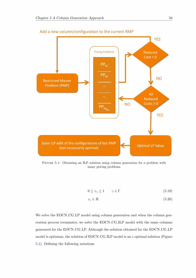


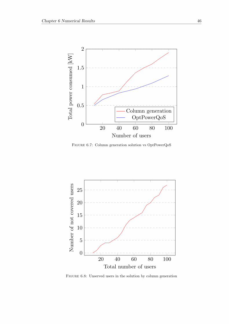


![LTE Radio Planning Using Atoll Radio Planning and ... · PDF fileestimation and optimization of an LTE network can be performed. 5. Methodology ... post-launch optimization[8]. But](https://static.documents.pub/doc/80x56/5a7a539e7f8b9a01528cfac2/lte-radio-planning-using-atoll-radio-planning-and-and-optimization-of-an-lte.jpg)