0

Energy Performance and Capital Expenditures

in Manufacturing Industries

Jasper Brinkerink a

Andrea Chegut b

Wilko Letterie c

Abstract:

Little is known about how firms change energy consumption over time. Yet to meet global climate change targets understanding how changes in firm investment impact environmental performance is important for policy makers and firms alike. To investigate the environmental performance of firms we measure the energy consumption and efficiency of firms in the Netherlands’ manufacturing industries before and after large capital expenditures over the 2000 to 2008 period. Unique to this data set, is that firm investment is decomposed into three streams: investment in buildings only, in equipment only or a simultaneous investment in both buildings and equipment. We find firms increase energy consumption when experiencing a simultaneous investment. However, after large capital expenditures energy efficiency increases. Further decomposition by firm types suggests that the building capital investments of firms active in high tech industries, energy intensive and low labor intensive industries does not concide with energy efficiency improvements, while energy efficiency does increase with capital expenditures in equipment. Hence, from a policy perspective targeted agreements that understand the production process of firms will require a differentiated strategy. In this case, voluntary agreements with firms, like those with equipment, may not shift energy consumption due to production demands. Third party verification to enhance transparency, subsidies or R&D tax credits may potentially yield better results.

Keywords: Investment, Energy Consumption, Energy Efficiency, Capital Expenditures JEL Classification: D22, D92, Q40, Q41

Acknowledgement: We thank David Geltner, Rogier Holtermans, Øivind Nilsen, Lyndsey Rolheiser and seminar participants at Maastricht University and MIT for useful comments during early stages of a project resulting in this paper. In addition, we are grateful to the referees of this journal for their suggestions on how to improve this study.

a Free University of Bozen-Bolzano, Faculty of Economics and Management, Centre for Family Business Management, Bolzano, Italy

b MIT, Center for Real Estate, Cambridge, USA c Maastricht University, School of Business and Economics, Department of Organization and Strategy, Maastricht, The Netherlands. Corresponding author, Email address: w.letterie@maastrichtuniversity.nl.

1

1. Introduction

Firm output in the industrial sector is very energy intensive. In the US, industrial sector energy

consumption in 2010 was 625 million tons of oil equivalent, or one third of total consumption (US

Energy Information Administration, 2014). Energy consumption in the EU is approximately 320

million tons of oil equivalent (European Environment Agency, 2014). Policy makers have sought

to change this energy intensity by incentivizing capital investments towards energy efficiency

through stricter building codes and more stringent equipment standards in the industrial sector

(Acemoglu et al., 2014; Acemoglu et al., 2009). Early results from Aroonruengsawat et al. (2012)

and Jacobsen and Kotchen (2013) document that improvements in residential building codes – that

impact new and redevelopment construction - decrease energy consumption by four to six percent.

Papineau (2013) has shown similar results for commercial buildings. These studies suggest that

stimulating capital investments embodying recent general technical change in energy efficiency for

industrial production and construction are ways in which policy could aim to attain environmental

goals.

Firm environmental performance is often measured in the literature and by policy makers by

looking at the output of firms across various toxicity-weighted pollutants - carbon, nitrate, sulfate

oxides. Overall, studies find that firms are decreasing their pollution over time (Cole et al., 2005;

Earnhart, 2004), but there are some sectors in which firms are not achieving environmental goals

(Gamper-Rabindran and Finger, 2013). However, we do not know the sources of environmental

performance surrounding firm investment activities: is it equipment, the buildings or some

combination of both? In addition, the literature on energy performance in buildings has documented

evidence of increased property value and decreased energy consumption after new building

development, but importantly these findings are divided from research investigating capital

2

expenditures at the firm level (Eicholtz et al., 2010; Dalton and Fuerst, 2017). By taking a firm-

level view of environmental performance that includes buildings and equipment as production

factors we are identifying firm-level challenges and capital expenditure areas for technological

progress in meeting environmental performance benchmarks.

To understand firm-level environmental performance we employ a multi-period event study to

measure the following outcomes. First, we investigate how the energy performance of firms active

in the energy intensive industrial sector develops around episodes of unusually large capital

investments – so called investment spikes (Power, 1998). Specifically, we compare the energy

consumption and energy efficiency of firms before, during, and after investment spikes in buildings

or equipment, or investment spikes in both capital types simultaneously. As such, the analysis

allows us to assess whether and how upgrading the capital stock of industrial firms contributes

towards attaining environmental goals concerning energy use and thus the emission of greenhouse

gasses. Second, we assess how firms’ operational efficiency develops around these same capital

investment spikes. By comparing the simultaneous development of firms’ energy performance and

of their operational efficiency surrounding capital investment spikes, we investigate if

environmetal goals conflict with – or rather complement – competitive goals. As such, we add to

literature adressing whether firms are able to combine “lean and green” production techniques (e.g.,

King and Lenox, 2001; Klassen and Wybark, 1999; Telle and Larsson, 2007).

We begin our analysis by developing a theoretical framework to guide our empirical analysis,

which looks at firm investment spikes across time periods and the arbitrary timing in investment

spike event patterns across firms to guide our empirical analysis of firm capital expenditures and

energy performance. The framework also enables us to understand how energy efficiency is related

to productivity of capital, price developments and a change in production technology. To

3

operationalize this model, we employ a micro-level panel dataset provided by Dutch Statistics

(CBS) covering the period 2000-2008. The dataset contains information concerning investment in

buildings and equipment. In addition, it provides data on production statistics and the energy

expenditures of firms. By identifying large capital expenditures we pinpoint major events at the

firm level (Power, 1998). Importantly, we distinguish between expenditures in buildings and

equipment. Furthermore, we allow for single expenditure events where the firm only adjusts one

type of capital, and we allow for a simultaneous expenditure where the firm makes a large

investment in both buildings and equipment. The purpose of discriminating between single and

simultaneous expenditures is that the latter are more likely to reflect expansionary efforts of the

firm, whereas single expenditures more likely refer to replacement of depreciated physical capital.

Our identification scheme makes it possible to measure how energy performance of the firm

behaves surrounding investment events. We examine firms in all sectors, but then decompose firms

into their innovation, labor and energy intensities. This is particularly important for understanding

and pinpointing problematic general sector trends and direct policy-making in specific sectors.

The main findings of our analysis are that when firms invest in both buildings and equipment

simultaneously energy consumption increases. This result signals that firms engaging in a

simultaneous investment are expanding the scale of their operations. Overall, energy consumption

is increasing with increased production. However, new buildings and new equipment tend to

incorporate technology consuming less energy. After investment has taken place energy efficiency

improves. Operational efficiency of firms improves when investing in equipment but it decreases

when investing in buildings. In particular, firms operating in energy and capital intensive industries

and high-tech industries face financial damage when investing in buildings, which is an area where

policy makers, engineers and firms can join to identify energy efficiency solutions.

4

The paper proceeds as follows. In the following section we provide a theoretical framework for

firm capital expenditures that could impact energy performance. Then, we describe the data

provided by CBS. In the next section, we explain our estimation strategy. Then, we depict our

results for all sectors, provide an industry cluster analysis, analyze operational efficiency and

consider a specific industry. We end with a conclusion and policy recommendations on the link

between firm investment, energy performance, and operational performance.

2. Theoretical Framework

In this section we start with a framework to guide our empirical analysis of firm-level energy

consumption and energy performance. The empirical strategy we employ is based on the notion of

investment spikes. These represent large capital expenditures. Our aim is to identify such large

expenditures as these most likely reflect major retooling or expansionary efforts of firms.

Investment data often also feature rather small expenditures. The model presented below does not

account for these. However, it can be adjusted easily to capture these small investment as well

without influencing the main results (Letterie and Pfann, 2007).

The presence of investment lumps can be explained as follows. Suppose that at time t a firm uses

two capital inputs – the stock of buildings is given by and the stock of equipment is given by

- to produce a non-storable output. We abstract from labour to ease exposition of the model,

without affecting the theoretical insights obtained. The value of the firm is given by:

(1)

BtK

EtK

( ) ( )0

, , , , ,s B E B B E Et t t s t s t s t s t s t s t s

sV F A K K C I K I Kb

¥

+ + + + + + +=

æ öé ù= E -ç ÷ë ûè øå

5

The term Et(.) indicates that expectations are taken with respect to information available at time t.

The discount rate satisfies . The expression denotes net

sales. We assume a Cobb-Douglas production technology with decreasing returns to scale,

, where Y, e and ϕ denote production, energy use and total factor

productivity, respectively. The price of energy is given by . The structural parameters satisfy

. Energy is a fully flexible factor of production. The isoelastic demand function is

given by , where . Then .

The term summarizes randomness in both total factor productivity and demand faced

by the firm.

Upon investment the firm incurs adjustment costs given by:

(2)

The function I(.) assumes the value 1 if the condition in brackets is satisfied and is equal to zero

otherwise. The adjustment cost function allows for convex costs. Their size is reflected by the

parameters and . Convex costs make large capital expenditures expensive and hence provide

an incentive to firms to smooth investment over time. The prices of the capital investment are

and , where for , . The purchase price for a unit

of capital c is pc+. When the firm sells one unit of capital the price received is pc-. As investment is

b 0 1b< < ( ), ,B E et t t t t t tF A K K pY p e= -

( ) ( ) ( )B Et t t t tY K K e

n µ kf=

etp

0 , , 1n µ k< <

( )1ej -=t t tp Y 1e > ( ) ( ) ( ) ( )( )

11

, ,B E B E et t t t t t t t t tF A K K K K e p e

n µ k ej f-

= -

11

t t tA ej f-

=

( )( )

( )

2

2

I 02

, , ,

I 02

BBB B B B Btt t t tB

tB B E Et t t t

EEE E E E Ett t t tE

t

Ibp I I KK

C I K I KIbp I I KK

a

a

é ùæ öê ú+ × ¹ + ×ç ÷ê úè ø= ê ú

æ öê ú+ + × ¹ + ×ç ÷ê úè øë û

Bb Eb

Btp

Etp { },c B EÎ ( ) ( )I 0 I 0c c c c c

t t tp p I p I+ -= × > + × <

6

partially irreversible, the purchase price of capital is higher than the resale price: pc+ > pc-. Fixed

costs are given by . In the model these costs are independent of the size of the

investment expenditure. In practice, such costs may capture increased managerial attention or the

loss of productivity due to the installation and adoption of new equipment, for instance

(Hamermesh and Pfann, 1996). Various empirical studies have found convincing empirical

evidence for this type of cost (see for example Cooper and Haltiwanger, 2006; Bloom, 2009;

Asphjell et al., 2014).1 We also assume these to be symmetric for simplicity. In fact, they are

independent of whether capital demand is positive or negative.

Investment in buildings and equipment is denoted by and , respectively. By conducting

investment the optimal size of the capital stocks, and , is reached. The parameters and

denote capital depreciation rates of buildings and equipment, respectively. Hence, capital is

governed by:

(3) ,

where . The firm decides upon and by maximising equation (1) subject to

equation (3). The shadow values of an additional unit of capital are given by:

(4)

where and measures the value change of the firm if the constraint in equation (3) is

1 Fixed costs have been assumed to be proportional to the scale of the firm measured by the stock of capital. We abstract from this scaling. For the arguments developed using the current model this assumption is innocuous.

and B Ea a

BtI

EtI

1BtK + 1

EtK +

Bd

Ed

( ), 1 , ,1c c c ci t i t i tK K Id+ = - +

{ },c B EÎ BtI

EtI

( ) ( )( ) ( )( )1 1 1 1 1 1 11

0 1 1

, , , , ,E 1

B E B B E Es t s t s t s t s t s t s t sc c s

t t c cs t s t s

F A K K C I K I KK K

l d b¥

+ + + + + + + + + + + + + ++

= + + + +

é ù¶ ¶ê ú= - -

¶ ¶ê úë ûå

{ },c B EÎ ctl

7

relaxed or if, equivalently, capital is increased by one unit. From equation (4) it can be seen that

the shadow values represent the expected present discounted value of the marginal profit of capital

minus the marginal adjustment costs in future periods. For we find that the first order

condition for investment is:

(5) .

According to Abel and Eberly (1994) factor demand equals:

(6) .

The firm determines whether to change the stock of capital for by evaluating:

(7) .

At the left hand side of equation (7) we see the expected benefits of investing. At the right hand

side the cost associated with the firm’s decisions is depicted. The expression approximates

the benefits due to which we obtain a closed-form solution. This expression holds exactly in a

continuous time framework with one production factor. Substituting equation (6) in equation (7)

we observe that adjusting the stock of capital is profitable if . Hence,

changing the amount of capital occurs if

(8)

{ },c B EÎ

0c

c c c tt t c

t

Ip bK

læ ö

- - =ç ÷è ø

c c ct t tc ct

I pK b

læ ö-= ç ÷è ø

{ },c B EÎ

( ),c c c ct t t tI C I Kl ³

c ct tIl

( )21 02

c c c ct t tc p K

bl a- ³ >

{ },c B EÎ

2 c cc c ct t c

t

bp AKal - > º

8

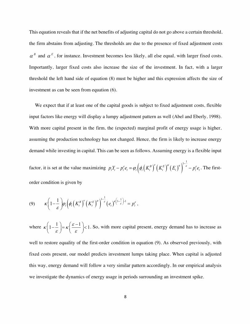
This equation reveals that if the net benefits of adjusting capital do not go above a certain threshold,

the firm abstains from adjusting. The thresholds are due to the presence of fixed adjustment costs

and , for instance. Investment becomes less likely, all else equal, with larger fixed costs.

Importantly, larger fixed costs also increase the size of the investment. In fact, with a larger

threshold the left hand side of equation (8) must be higher and this expression affects the size of

investment as can be seen from equation (6).

We expect that if at least one of the capital goods is subject to fixed adjustment costs, flexible

input factors like energy will display a lumpy adjustment pattern as well (Abel and Eberly, 1998).

With more capital present in the firm, the (expected) marginal profit of energy usage is higher,

assuming the production technology has not changed. Hence, the firm is likely to increase energy

demand while investing in capital. This can be seen as follows. Assuming energy is a flexible input

factor, it is set at the value maximizing . The first-

order condition is given by

(9) ,

where . So, with more capital present, energy demand has to increase as

well to restore equality of the first-order condition in equation (9). As observed previously, with

fixed costs present, our model predicts investment lumps taking place. When capital is adjusted

this way, energy demand will follow a very similar pattern accordingly. In our empirical analysis

we investigate the dynamics of energy usage in periods surrounding an investment spike.

Ba Ea

( ) ( ) ( )( )11

e B E et t t t t t t t t t tp Y p e K K E p e

n µ k ej f-

- = -

( ) ( )( ) ( )11 11 111 B E e

t t t t t tK K e pn µ ke

ek j fe

- æ ö- -ç ÷è ø

æ ö- =ç ÷è ø

1 11 1ek ke e

-æ ö æ ö- = <ç ÷ ç ÷è ø è ø

9

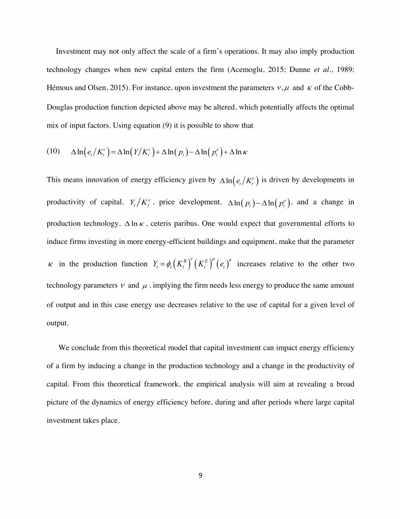
Investment may not only affect the scale of a firm’s operations. It may also imply production

technology changes when new capital enters the firm (Acemoglu, 2015; Dunne et al., 1989;

Hémous and Olsen, 2015). For instance, upon investment the parameters and of the Cobb-

Douglas production function depicted above may be altered, which potentially affects the optimal

mix of input factors. Using equation (9) it is possible to show that

(10)

This means innovation of energy efficiency given by is driven by developments in

productivity of capital, , price development, , and a change in

production technology, , ceteris paribus. One would expect that governmental efforts to

induce firms investing in more energy-efficient buildings and equipment, make that the parameter

in the production function increases relative to the other two

technology parameters and , implying the firm needs less energy to produce the same amount

of output and in this case energy use decreases relative to the use of capital for a given level of

output.

We conclude from this theoretical model that capital investment can impact energy efficiency

of a firm by inducing a change in the production technology and a change in the productivity of

capital. From this theoretical framework, the empirical analysis will aim at revealing a broad

picture of the dynamics of energy efficiency before, during and after periods where large capital

investment takes place.

,n µ k

( ) ( ) ( ) ( )ln ln ln ln lnc c et t t t te K Y K p p kD = D +D -D +D

( )ln ct te KD

ct tY K ( ) ( )ln ln e

t tp pD -D

lnkD

k ( ) ( ) ( )B Et t t t tY K K e

n µ kf=

n µ

10

3. Data Description

The Netherlands is a country that provides a particularly rich data environment for analysing

building code standards. With respect to buildings, according to Dutch building codes firms need

to comply with energy efficiency standards. In fact, the last two decades there were three policy

instruments directed at the building sector in the Netherlands. Building codes and regulatory

instruments were started in the Energy Performance Standard for Buildings in 1995. Further

guidance, educational materials and subsidies were developed in the Energy Performance advice

and the More with Less Program (International Energy Agency, 2014). Hence, if a building is

redeveloped or developed, it must meet standards that satisfy energy efficiency improvements.

In regards to equipment there were four voluntary approach agreements with energy intensive

manufacturers over the same time period. Notably, this includes The Energy Efficiency

Benchmarking Covenant in 1999, which was later superseded by the Long-term Agreement on

Energy Efficiency for enterprises participating in the EU Emissions Trading System. This covenant

aims to enhance manufacturing energy efficiency in equipment (International Energy Agency,

2014).

We aim to discern whether new buildings and equipment lead towards cleaner technology.

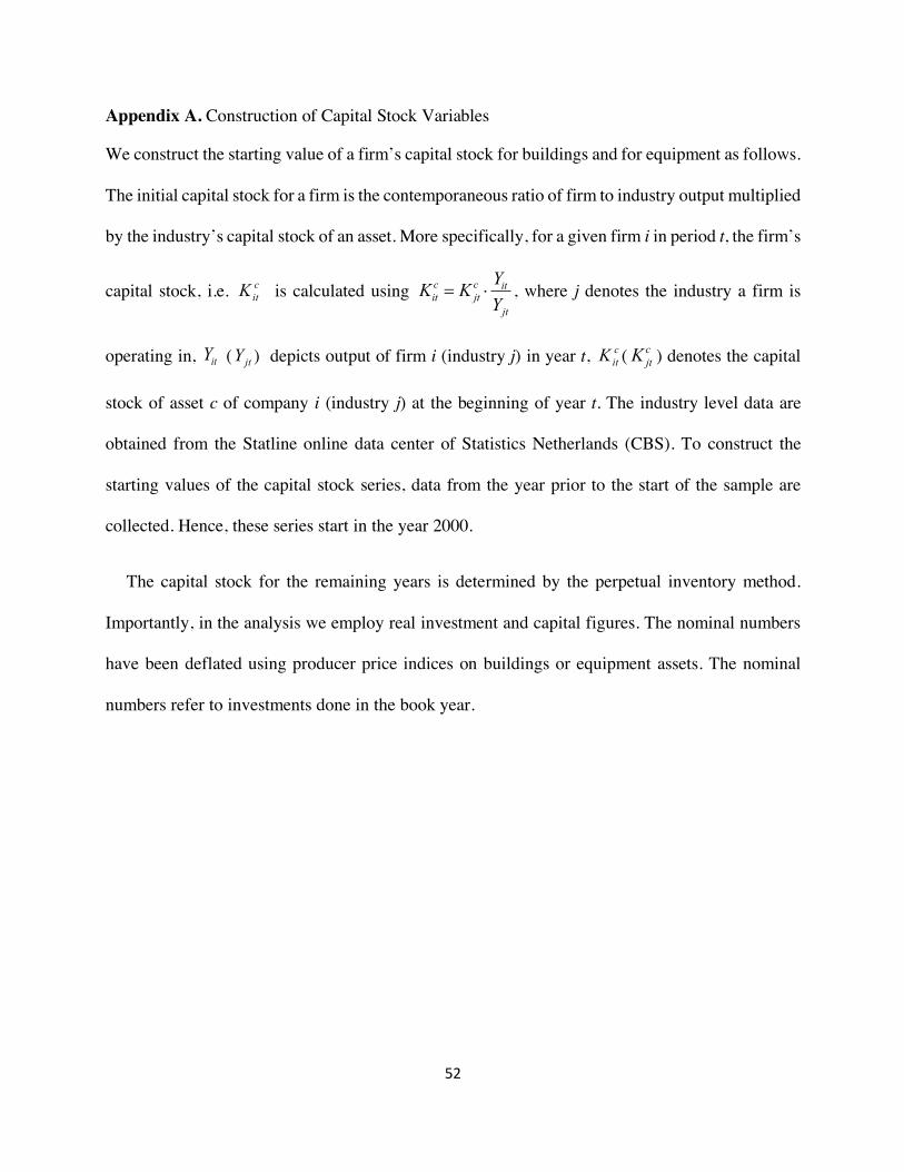
A unique opportunity provided by Statistics Netherlands (CBS) data is that both firm investment

and energy consumption data is collected at the firm level. Moreover, the data enables the

decomposition of the type of capital investment, e.g., buildings and equipment. CBS collects data

on production statistics and investment figures at the firm level on an annual basis. A random

selection of all Dutch companies employing less than 50 people is sent questionnaires and all firms

11

with 50 or more employees receive the survey.2 The data sets on production statistics and

investments of the manufacturing sector are merged using a firm specific identifier. We focus on

regular firm investment intensity dynamics and not on extreme events like divestments or mergers.

For that reason we construct a balanced panel. In this way, the panel conservatively controls for

firm entry and exit, major (dis)investment decisions like mergers, acquisitions, bankruptcies and/or

geographic relocations. In addition, as we want to employ empirical data, imputed observations are

disregarded. We also removed the 1% largest investment ratios to obtain the final data, in order to

prevent our findings from being affected by extreme outliers. The panel data set isolates investment

behaviour for 2000 to 2008. We have chosen to limit our data up until 2008, as from 2009 onwards

CBS used another operational definition of the unit of observation. We disregard years prior to

2000 as the balanced nature of the data would imply an additional loss of observations we like to

avoid. Our data concern 652 firms and the total number of yearly observations equals 5,868. This

sample is representative of large firms, those with 50 or more employees in the Netherlands and

our data has close to 30 percent of the large firm sample.3

Firms have been found to conduct investment in a lumpy fashion. Rather than smoothing

investment over time, micro-level data have revealed that investment by firms is often concentrated

in short time episodes. In this study we will focus on such bursts of capital adjustment as these

events represent major retooling or expansionary efforts of firms (Letterie et al., 2010). To

investigate micro-level consequences of such events, various studies have proposed a definition of

2 Sampling strategies and collection methods of Statistics Netherlands can be obtained from: http://www.cbs.nl/nl-NL/menu/themas/industrie-energie/methoden/dataverzameling/korte-onderzoeksbeschrijvingen/productie-statistiek.htm (in Dutch only). 3 One limitation of our data is that they do not allow us to disentangle or identify substitution or transfer of activities etc. between plants within one firm.

12

investment spikes. Some have employed an absolute spike definition. In that case, if the investment

ratio is larger than an ad hoc value such as 0.2, the observation is refered to as an investment spike

(see for instance Cooper et al., 1999; Sakellaris, 2004). A drawback of the absolute spike definition

is that it is not well suited to capture sporadic bursts of investment. Furthermore, we have

experienced that when using this absolute spike definition for buildings we find rather few spikes.

For that reason we employ an event identification scheme for investments in both equipment and

buildings, which does not suffer from these disadvantages. This classification method is refered to

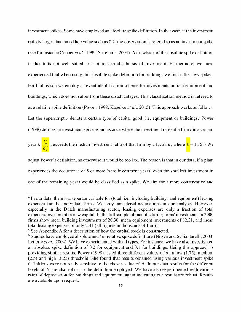
as a relative spike definition (Power, 1998; Kapelko et al., 2015). This approach works as follows.

Let the superscript z denote a certain type of capital good, i.e. equipment or buildings.4 Power

(1998) defines an investment spike as an instance where the investment ratio of a firm ! in a certain

year t, , exceeds the median investment ratio of that firm by a factor ", where = 1.75.5,6 We

adjust Power’s definition, as otherwise it would be too lax. The reason is that in our data, if a plant

experiences the occurrence of 5 or more ‘zero investment years’ even the smallest investment in

one of the remaining years would be classified as a spike. We aim for a more conservative and

4 In our data, there is a separate variable for (total; i.e., including buildings and equipment) leasing expenses for the individual firms. We only considered acquisitions in our analysis. However, especially in the Dutch manufacturing sector, leasing expenses are only a fraction of total expenses/investment in new capital. In the full sample of manufacturing firms' investments in 2000 firms show mean building investments of 20.38, mean equipment investments of 82.21, and mean total leasing expenses of only 2.41 (all figures in thousands of Euro). 5 See Appendix A for a description of how the capital stock is constructed. 6 Studies have employed absolute and / or relative spike definitions (Nilsen and Schiantarelli, 2003; Letterie et al., 2004). We have experimented with all types. For instance, we have also investigated an absolute spike definition of 0.2 for equipment and 0.1 for buildings. Using this approach is providing similar results. Power (1998) tested three different values of , a low (1.75), medium (2.5) and high (3.25) threshold. She found that results obtained using various investment spike definitions were not really sensitive to the chosen value of . In our data results for the different levels of are also robust to the definition employed. We have also experimented with various rates of depreciation for buildings and equipment, again indicating our results are robust. Results are available upon request.

zitzit

IK

q

q

qq

13

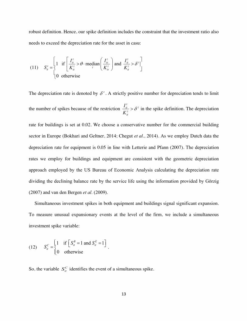
robust definition. Hence, our spike definition includes the constraint that the investment ratio also

needs to exceed the depreciation rate for the asset in casu:

(11)

The depreciation rate is denoted by . A strictly positive number for depreciation tends to limit

the number of spikes because of the restriction in the spike definition. The depreciation

rate for buildings is set at 0.02. We choose a conservative number for the commercial building

sector in Europe (Bokhari and Geltner, 2014; Chegut et al., 2014). As we employ Dutch data the

depreciation rate for equipment is 0.05 in line with Letterie and Pfann (2007). The depreciation

rates we employ for buildings and equipment are consistent with the geometric depreciation

approach employed by the US Bureau of Economic Analysis calculating the depreciation rate

dividing the declining balance rate by the service life using the information provided by Görzig

(2007) and van den Bergen et al. (2009).

Simultaneous investment spikes in both equipment and buildings signal significant expansion.

To measure unusual expansionary events at the level of the firm, we include a simultaneous

investment spike variable:

(12) .

So, the variable identifies the event of a simultaneous spike.

1 if median and

0 otherwise

z z zzit i it

z z z zit it i it

I I IS K K K

t

tt

q dì é ùæ ö

> × >ï ê úç ÷= í è øë ûïî

zd

zzit

zit

IK

d>

1 if 1 and 1

0 otherwise

B Eit itC

it

S SS

ì é ù= =ï ë û= íïî

CitS

14

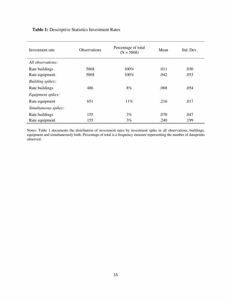
A set of descriptive statistics for the investment spikes (in buildings, equipment, or a

combination of both) is provided in Table 1. We observe that the frequency of spikes is 8 and 11

percent for buildings and equipment respectively. Simultaneous spikes occur in 3 percent of the

data. The mean investment rate for equipment during simultaneous spikes is higher than in the

absence of a spike in buildings, hinting at an expansionary effort of the firm.

15

Table 1: Descriptive Statistics Investment Rates

Investment rate Observations Percentage of total (N = 5868) Mean Std. Dev.

All observations: Rate buildings 5868 100% .011 .030 Rate equipment 5868 100% .042 .053 Building spikes: Rate buildings 486 8% .068 .054 Equipment spikes: Rate equipment 651 11% .216 .017 Simultaneous spikes: Rate buildings 155 3% .070 .047 Rate equipment 155 3% .240 .199

Notes: Table 1 documents the distribution of investment rates by investment spike in all observations, buildings, equipment and simultaneously both. Percentage of total is a frequency measure representing the number of datapoints observed.

16

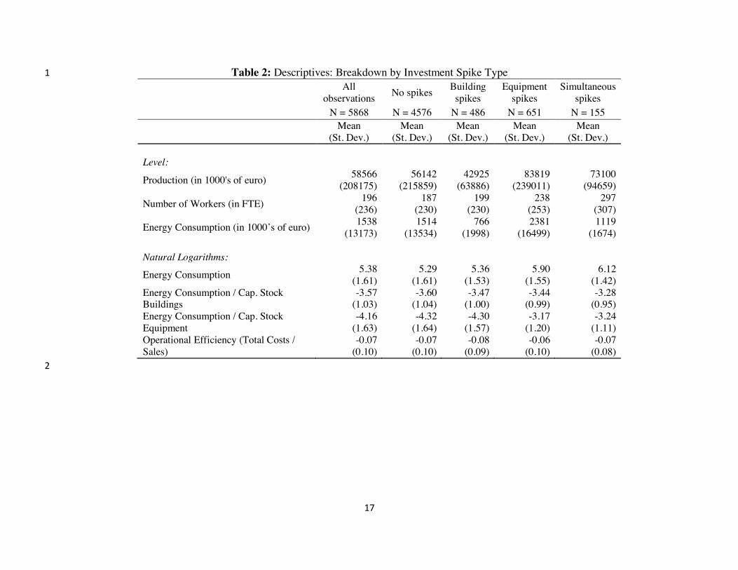
In Table 2 we depict the mean and standard deviation of energy usage, energy efficiency and

operational efficiency under the scenarios of (i) all observations, (ii) no investment spikes, and in

case of (iii) single spikes in buildings, (iv) single spikes in equipment and (v) simultaneous spikes.

Note that we have deflated production values and energy expenses by the annual production and

energy Producer Price Indices (PPIs) available at Statistics Netherlands (CBS) Statline online

datacenter. The base year is 2000. The dependent variables we use in the empirical analysis are in

natural logs.

17

Table 2: Descriptives: Breakdown by Investment Spike Type 1

All

observations No spikes Building spikes

Equipment spikes

Simultaneous spikes

N = 5868 N = 4576 N = 486 N = 651 N = 155

Mean

(St. Dev.) Mean

(St. Dev.) Mean

(St. Dev.) Mean

(St. Dev.) Mean

(St. Dev.)

Level:

Production (in 1000's of euro) 58566 (208175)

56142 (215859)

42925 (63886)

83819 (239011)

73100 (94659)

Number of Workers (in FTE) 196 (236)

187 (230)

199 (230)

238 (253)

297 (307)

Energy Consumption (in 1000’s of euro) 1538 (13173)

1514 (13534)

766 (1998)

2381 (16499)

1119 (1674)

Natural Logarithms:

Energy Consumption 5.38 (1.61)

5.29 (1.61)

5.36 (1.53)

5.90 (1.55)

6.12 (1.42)

Energy Consumption / Cap. Stock Buildings

-3.57 (1.03)

-3.60 (1.04)

-3.47 (1.00)

-3.44 (0.99)

-3.28 (0.95)

Energy Consumption / Cap. Stock Equipment

-4.16 (1.63)

-4.32 (1.64)

-4.30 (1.57)

-3.17 (1.20)

-3.24 (1.11)

Operational Efficiency (Total Costs / Sales)

-0.07 (0.10)

-0.07 (0.10)

-0.08 (0.09)

-0.06 (0.10)

-0.07 (0.08)

2

18

Table 2 reveals firms not experiencing a spike at all are relatively small as measured by the level

of production and number of workers. Also firms only conducting a large investment in buildings

tend to be rather small. Firms that are involved with large investments in equipment are larger on

average. Firms just conducting major investments in buildings do not use a lot of energy, compared

to firms investing in equipment.

With respect to energy efficiency we see from the bottom part of Table 2 that firms engaging in

equipment spikes are more efficient in energy usage as reflected by energy consumption divided

by the capital stock of equipment. In contrast, firms displaying building spikes are more efficient

in energy usage as reflected by energy consumption divided by the capital stock of buildings. Firms

not conducting major investment episodes typically belong to the least energy efficient groups, by

all measures. Finally, we analyze the variable operational efficiency as measured by the ratio of

cost to sales. Note that the cost variable does not include investment expenditures. It appears our

measure of firm efficiency is relatively stable and independent of the investment profile of the firm.

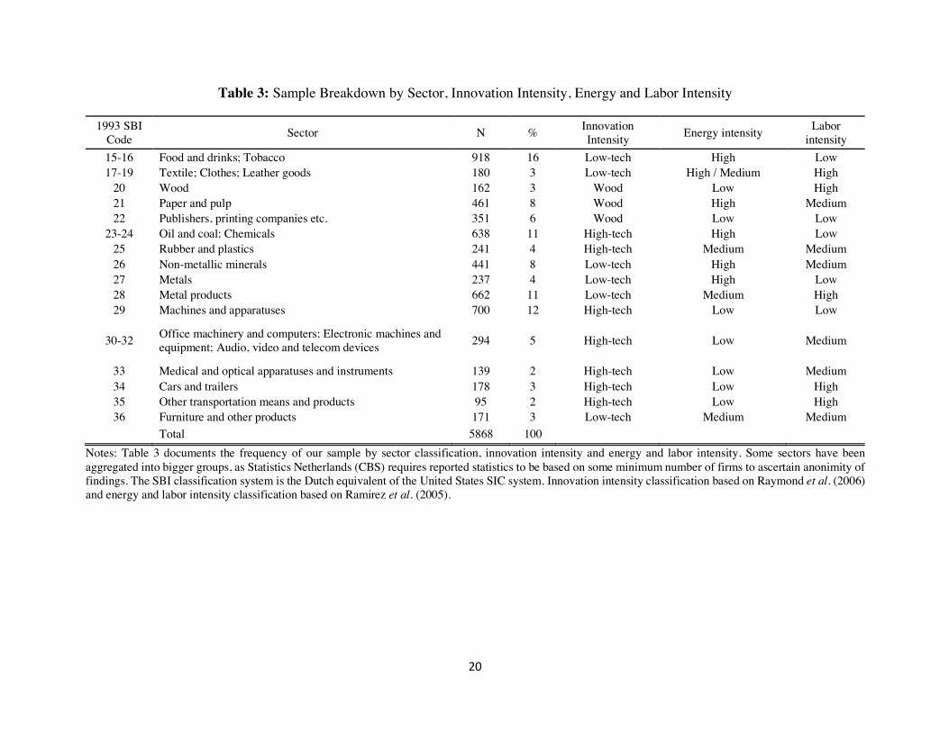
To identify high- and low-tech industry categories in Dutch manufacturing we follow Raymond

et al. (2006). A low-tech firm is characterized by a low propensity to engage in innovation-seeking

activities like R&D and innovation subsidy achievement. Following Raymond et al., wood-based

industries are characterized as distinctively non-innovative. Labor and energy intensity industry

groupings are based on Ramirez et al. (2005). Table 3 identifies how the sample firms are classified

by innovation, energy and labor intensity. High-tech and low-tech sectors represent 39 and 45

percent of the sample, respectively. High-tech firms are predominantly active in the Oil and coal,

Chemicals, Transportation, and Machines and apparatuses sectors. High-, medium- and low-labor-

intensive industries reflect 22, 30 and 49 percent of the sample, respectively. Low-labor-intensive

industries are split almost evenly between high-tech and low-tech industries. High-, medium- and

19

low-energy-intensive firms represent 47, 21 and 33 percent of the sample data, respectively.

Energy-intensive firms can be found in industries like Food, drinks and tobacco, Paper and pulp,

Oil, coal and chemicals, Non-metallic minerals and Metals.

20

Table 3: Sample Breakdown by Sector, Innovation Intensity, Energy and Labor Intensity

1993 SBI Code

Sector N % Innovation Intensity

Energy intensity Labor intensity

15-16 Food and drinks; Tobacco 918 16 Low-tech High Low 17-19 Textile; Clothes; Leather goods 180 3 Low-tech High / Medium High

20 Wood 162 3 Wood Low High 21 Paper and pulp 461 8 Wood High Medium 22 Publishers, printing companies etc. 351 6 Wood Low Low

23-24 Oil and coal; Chemicals 638 11 High-tech High Low 25 Rubber and plastics 241 4 High-tech Medium Medium 26 Non-metallic minerals 441 8 Low-tech High Medium 27 Metals 237 4 Low-tech High Low 28 Metal products 662 11 Low-tech Medium High 29 Machines and apparatuses 700 12 High-tech Low Low

30-32 Office machinery and computers; Electronic machines and equipment; Audio, video and telecom devices 294 5 High-tech Low Medium

33 Medical and optical apparatuses and instruments 139 2 High-tech Low Medium 34 Cars and trailers 178 3 High-tech Low High 35 Other transportation means and products 95 2 High-tech Low High 36 Furniture and other products 171 3 Low-tech Medium Medium

Total 5868 100 Notes: Table 3 documents the frequency of our sample by sector classification, innovation intensity and energy and labor intensity. Some sectors have been aggregated into bigger groups, as Statistics Netherlands (CBS) requires reported statistics to be based on some minimum number of firms to ascertain anonimity of findings. The SBI classification system is the Dutch equivalent of the United States SIC system. Innovation intensity classification based on Raymond et al. (2006) and energy and labor intensity classification based on Ramirez et al. (2005).

21

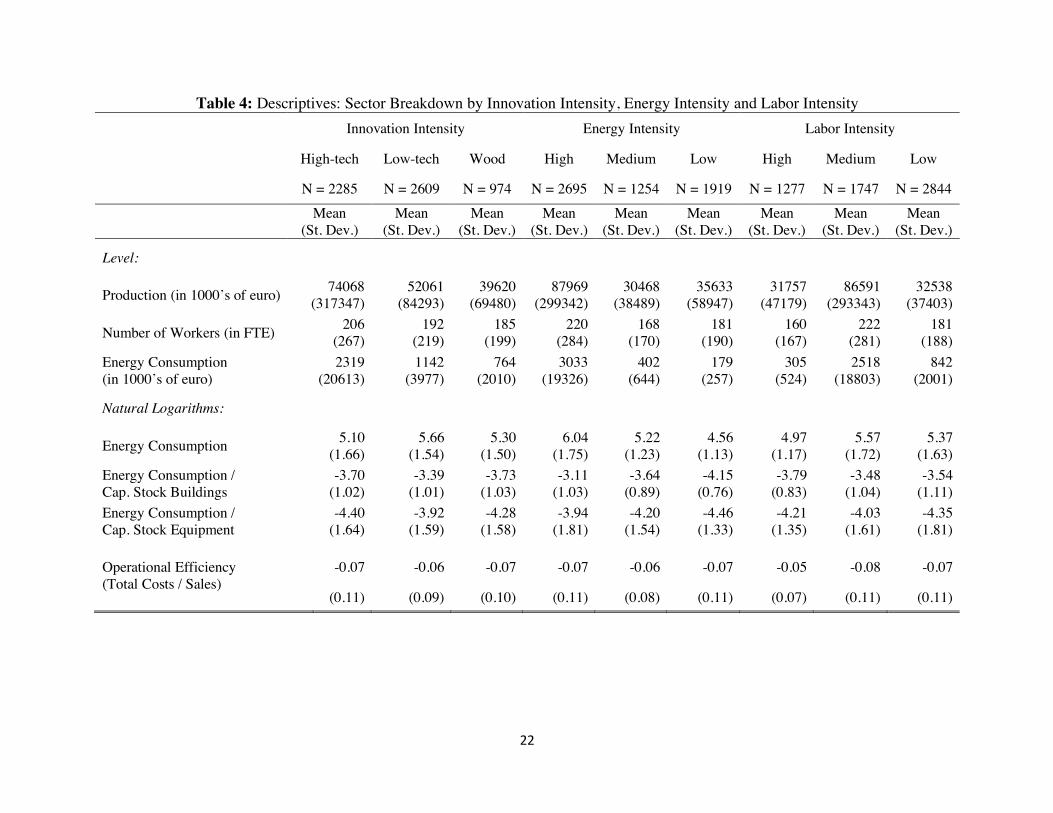
Table 4 provides summary statistics on how the variables of interest vary across sectors if we

break them down according to innovation intensity, energy intensity and labor intensity. The

bottom part of the table shows that on average firms with the highest energy consumption operate

in sectors characterized by low innovation intensity, high energy intensity and medium / low labor

intensity. Typically, in high-tech industries one can find the most energy-efficient firms. Firms in

sectors with high labor intensity on average display high energy efficiency as measured by low

energy consumption per unit of buildings. In contrast, firms characterized by low labor intensity

on average score high on energy efficiency as indicated by a low consumption of energy per unit

of equipment.

22

Table 4: Descriptives: Sector Breakdown by Innovation Intensity, Energy Intensity and Labor Intensity Innovation Intensity Energy Intensity Labor Intensity

High-tech Low-tech Wood High Medium Low High Medium Low

N = 2285 N = 2609 N = 974 N = 2695 N = 1254 N = 1919 N = 1277 N = 1747 N = 2844

Mean (St. Dev.)

Mean (St. Dev.)

Mean (St. Dev.)

Mean (St. Dev.)

Mean (St. Dev.)

Mean (St. Dev.)

Mean (St. Dev.)

Mean (St. Dev.)

Mean (St. Dev.)

Level:

Production (in 1000’s of euro) 74068 (317347)

52061 (84293)

39620 (69480)

87969 (299342)

30468 (38489)

35633 (58947)

31757 (47179)

86591 (293343)

32538 (37403)

Number of Workers (in FTE) 206 (267)

192 (219)

185 (199)

220 (284)

168 (170)

181 (190)

160 (167)

222 (281)

181 (188)

Energy Consumption (in 1000’s of euro)

2319 (20613)

1142 (3977)

764 (2010)

3033 (19326)

402 (644)

179 (257)

305 (524)

2518 (18803)

842 (2001)

Natural Logarithms:

Energy Consumption 5.10 (1.66)

5.66 (1.54)

5.30 (1.50)

6.04 (1.75)

5.22 (1.23)

4.56 (1.13)

4.97 (1.17)

5.57 (1.72)

5.37 (1.63)

Energy Consumption / Cap. Stock Buildings

-3.70 (1.02)

-3.39 (1.01)

-3.73 (1.03)

-3.11 (1.03)

-3.64 (0.89)

-4.15 (0.76)

-3.79 (0.83)

-3.48 (1.04)

-3.54 (1.11)

Energy Consumption / Cap. Stock Equipment

-4.40 (1.64)

-3.92 (1.59)

-4.28 (1.58)

-3.94 (1.81)

-4.20 (1.54)

-4.46 (1.33)

-4.21 (1.35)

-4.03 (1.61)

-4.35 (1.81)

Operational Efficiency (Total Costs / Sales)

-0.07

(0.11)

-0.06

(0.09)

-0.07

(0.10)

-0.07

(0.11)

-0.06

(0.08)

-0.07

(0.11)

-0.05

(0.07)

-0.08

(0.11)

-0.07

(0.11)

23

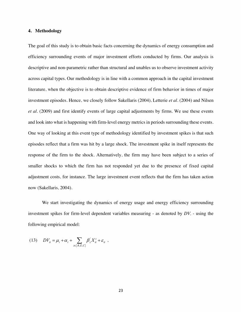
4. Methodology

The goal of this study is to obtain basic facts concerning the dynamics of energy consumption and

efficiency surrounding events of major investment efforts conducted by firms. Our analysis is

descriptive and non-parametric rather than structural and unables us to observe investment activity

across capital types. Our methodology is in line with a common approach in the capital investment

literature, when the objective is to obtain descriptive evidence of firm behavior in times of major

investment episodes. Hence, we closely follow Sakellaris (2004), Letterie et al. (2004) and Nilsen

et al. (2009) and first identify events of large capital adjustments by firms. We use these events

and look into what is happening with firm-level energy metrics in periods surrounding these events.

One way of looking at this event type of methodology identified by investment spikes is that such

episodes reflect that a firm was hit by a large shock. The investment spike in itself represents the

response of the firm to the shock. Alternatively, the firm may have been subject to a series of

smaller shocks to which the firm has not responded yet due to the presence of fixed capital

adjustment costs, for instance. The large investment event reflects that the firm has taken action

now (Sakellaris, 2004).

We start investigating the dynamics of energy usage and energy efficiency surrounding

investment spikes for firm-level dependent variables measuring - as denoted by DVit - using the

following empirical model:

(13) ,

{ }

'

, ,

zit i t z it it

z B E CDV Xµ a b e

Î

= + + +å

24

where is a firm specific effect, is a year dummy vector capturing potential macro-economic

developments and denotes an idiosyncratic error. Our approach resembles an event study

(Wooldrige 2013) where the goal is to estimate the effect of an event, a policy program for instance,

on an outcome variable of interest. Typically, such studies allow for exogenous treatment variables

such that causal inferences can be made. In our study the assumption of strict exogeneity of the

events, which are identified by the occurrence of investment episodes, is violated. Hence, our

estimates should be interpreted carefully with regards to causality. They provide us with a

description of dynamic patters of plant-level energy metrics surrounding major capital adjustments

in plants.

The vector captures the event for both capital types (i.e. buildings where z=B and

equipment where z=E), as well as for a simultaneous spike episode (where z=C) in case a

simultaneous investment spike in buildings and equipment takes place (i.e. where ):

(14)

,

iµ ta

ite

zitX

1B Eit itS S= =

BitXé ù =ë û

( )( ) ( )( ) ( )

( )( ) ( )( )( ) ( )( )( )( ) { }

1 2 21

1 12

3

4 1 1

5 1 2 2

61 2 3

1 1 1

1 1

1

1 1

1 1 1

1 1 1 max

B B B Eit it it itB

itB B E

B it it itit

B EBit itit

B B B Eit it it itB B B B Eit it it it itB

B B B Bitit it it it

S S S SX

S S SXS SX

X S S SX S S S SX S S S S tt

+ + +

+ +

- -

- - -

- - £ -

é - - -é ù êê ú ê - -ê ú êê ú ê -ê ú ê=ê ú ê - -ê úê ú - - -ê úë û - - - ×ë

ùúúúúúú

ê úê úê úê ú

û

25

(15)

,

(16)

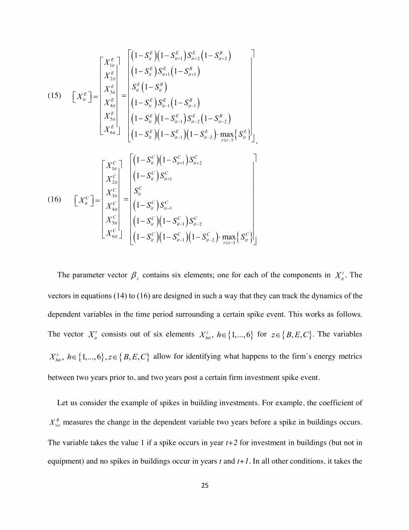
The parameter vector contains six elements; one for each of the components in . The

vectors in equations (14) to (16) are designed in such a way that they can track the dynamics of the

dependent variables in the time period surrounding a certain spike event. This works as follows.

The vector consists out of six elements for . The variables

allow for identifying what happens to the firm’s energy metrics

between two years prior to, and two years post a certain firm investment spike event.

Let us consider the example of spikes in building investments. For example, the coefficient of

measures the change in the dependent variable two years before a spike in buildings occurs.

The variable takes the value 1 if a spike occurs in year t+2 for investment in buildings (but not in

equipment) and no spikes in buildings occur in years t and t+1. In all other conditions, it takes the

EitXé ù =ë û

( )( ) ( )( ) ( )

( )( ) ( )( )( ) ( )( )( )( ) { }

1 2 21

1 12

3

4 1 1

5 1 2 2

61 2 3

1 1 1

1 1

1

1 1

1 1 1

1 1 1 max

E E E Bit it it itE

itE E B

E it it itit

E BEit itit

E E E Bit it it itE E E E Bit it it it itE

E E E Eitit it it it

S S S SX

S S SXS SX

X S S SX S S S SX S S S S tt

+ + +

+ +

- -

- - -

- - £ -

é - - -é ù êê ú ê - -ê ú êê ú ê -ê ú ê=ê ú ê - -ê úê ú - - -ê úë û - - - ×ë

ùúúúúúú

ê úê úê úê ú

û

CitXé ù =ë û

( )( )( )

( )( )( )( )( )( ) { }

1 21

12

3

14

5 1 2

61 2 3

1 1

1

1

1 1

1 1 1 max

C C CC it it itit

C CC it itit

CCitit

C CCit itit

C C C Cit it it itC

C C C Citit it it it

S S SX

S SXSX

S SXX S S SX S S S S tt

+ +

+

-

- -

- - £ -

é ù- -é ù ê úê ú ê ú-ê ú ê úê ú ê úê ú ê ú=ê ú -ê úê ú ê úê ú - -ê úê ú ê úë û - - - ×ê úë û

zbzitX

zitX { }, 1,...,6z

hitX hÎ { }, ,z B E CÎ

{ } { }, 1,...,6 , , ,Î ÎzhitX h z B E C

1BitX

26

value 0. The parameter estimate for variable measures the change in DVit one year before a

spike in buildings. The variable takes the value 1 if a spike in buildings occurs in year t+1 (but not

in equipment), and no spikes in buildings occur in year t; alternatively it assumes the value 0. To

measure changes in the dependent variable at the time of a spike we employ . It assumes the

value 1 if a spike in buildings occurs in year t, and there is no spike in equipment in t. It will be 0

otherwise. The variables and are similar to and , though they indicate a spike in

year t-1 (t-2) rather than t+1 (t+2). Thus, these variables identify what happens one and two years

after a spike event, respectively. Finally, using we capture the change in DVit after three or

more years. The variable takes the value 1 if a spike occurs before year t-2, but not in t-2, t-1 and

t. The vectors and are analogous to . The parameter estimates for vector identify

adjustment of DVit surrounding spikes in equipment only. Likewise, coefficients of measure

adjustment of DVit surrounding simultaneous spikes in both buildings and equipment.

Estimating equation (13) yields regression coefficients captured by the vector with six

elements for independent variables . They identify the adjustment of the

dependent variable DVit for firms i that are experiencing a spike in buildings, equipment or are

experiencing a combined spike. These estimates measure the difference between a firm conducting

a major investment and a firm that is not experiencing a spike. Due to the fixed effects specification

the estimates identify the within variation of the dependent variable across various investment

experiences of firms. As the dependent variables are in natural logarithms, from the coefficients in

the vector percentage differences can be calculated in the dependent variable between firms

that are, and firms that are not in the situation described by an element For example, consider

2BitX

3BitX

4BitX 5

BitX 2

BitX 1

BitX

6BitX

EitX

CitX

BitX

EitX

CitX

zb

{ }, , ,zitX z B E CÎ

zb

.zitX

27

as a dependent variable the natural logarithm of energy consumption in year t. Suppose the

parameter estimate for equals 0.01. Then a firm that simultaneously invested in equipment

and structures in the previous year, i.e. period t-1, experiences energy consumption approximately

1 percent higher in year t than a firm that did not conduct a simultaneous spike in the previous year,

correcting for firm specific heterogeneity.

As long as an investment spike is observed in the timeframe 2000-2008, we also define all those

other elements of the vector that can be observed subject to data availability. As an example,

for an investment spike in equipment in the year 2007, we set , , and

equal to 1, but logically do not define and , as they fall outside of our observation

window. Let us now say a firm experienced an investment spike in 2009. In that case, and

should be equal to 1. However, they are held to 0 in our data, because we cannot observe

2009. This measurement error will likely bias the findings downward to zero. Hence, this adds

some conservativeness to our conclusions.

Hausman tests on all models indicate that all dependent variables required a fixed effects

specification. The models are estimated using fixed effects, within estimators. Within estimators

are more efficient than first differencing, assuming i.i.d. idiosyncratic error terms . Since we do

not (for example) include any lagged variables in the regression, this is a safe assumption after

averaging out the fixed effects. Note, we do not intend to estimate a model obtaining causal

insights. We rather aim at describing dynamic patterns of some key firm level variables. We

abstract from time-invariant variables as they are omitted from the model due to differencing fixed

effects.

4CitX

zitX

1 2005EiX 2 2006

EiX 3 2007

EiX 4 2008

EiX

5 2009EiX 6 2010

EiX

1 2007EiX

2 2008EiX

ite

28

5. Results

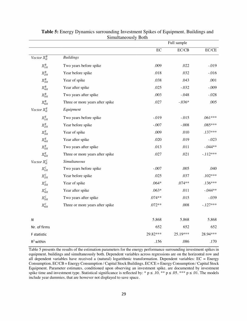
In Table 5 we present our results reflecting the dynamics of firm level energy performance metrics

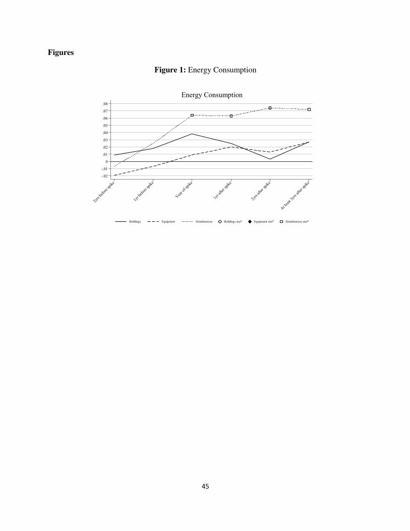
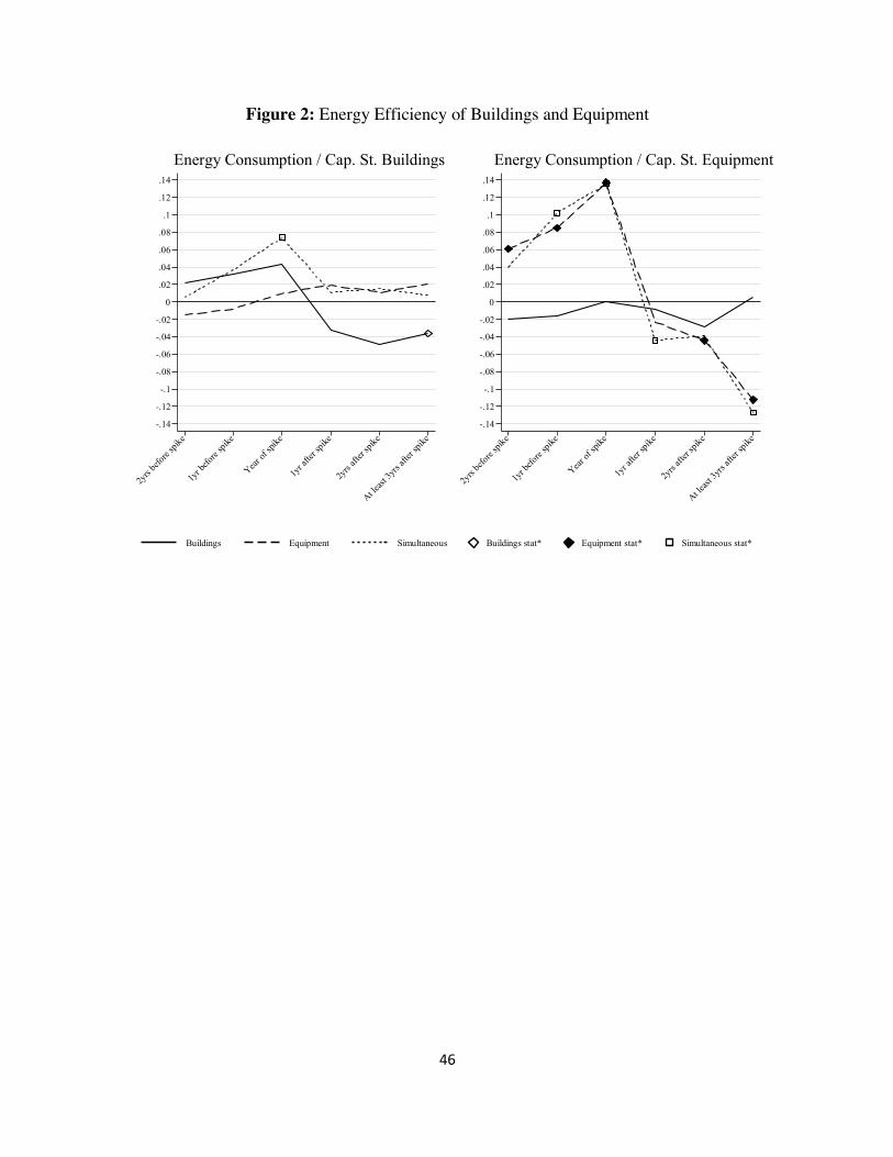
surrounding investment spikes for the full sample. Based on these results we constructed Figures

1 and 2. These figures depict how three energy performance metrics behave around specific

investment events for the full sample. We observe that energy consumption tends to increase by

around 7 percent when a firm experiences a simultaneous spike. This result is statistically

significant. Energy usage displays no major changes in case firms conducting a single spike.

Depicted in Figure 2, Energy Consumption per Capital Stock of Buildings, energy efficiency does

improve by 4 percent after three or more years when a firm experiences a spike in buildings. In

Figure 2, Energy Consumption per Capital Stock of Equipment shows that three or more years after

either a simultaneous spike or a single spike in equipment the firm’s energy efficiency improves

by even 12 percent. Strikingly, before these spikes the energy efficiency metrics indicate relatively

low performance, indicating that the firms’ production processes have become more energy

inefficient potentially due to working at full capacity or due to aging. Thus, we see from Figure 1

that firms use more energy after conducting major investment efforts in both buildings and

equipment simultaneously. However, Figure 2 reveals they do use the energy more efficiently after

the investments have taken place. Even though the scale of operations tends to increase, especially

in case of a simultaneous spike, firms produce using more energy efficient processes. In fact, in the

case of a single spike in buildings, the energy consumption per unit of buildings decreases.

Furthermore, if a single or simultaneous spike occurs including equipment, energy usage per unit

of equipment decreases.

29

Table 5: Energy Dynamics surrounding Investment Spikes of Equipment, Buildings and Simultaneously Both

Full sample

EC EC/CB EC/CE

Vector !"#$ Buildings

!%"#$ Two years before spike .009 .022 -.019

!&"#$ Year before spike .018 .032 -.016

!'"#$ Year of spike .038 .043 .001

!("#$ Year after spike .025 -.032 -.009

!)"#$ Two years after spike .003 -.048 -.028

!*"#$ Three or more years after spike .027 -.036* .005

Vector !"#+ Equipment

!%"#+ Two years before spike -.019 -.015 .061***

!&"#+ Year before spike -.007 -.008 .085***

!'"#+ Year of spike .009 .010 .137***

!("#+ Year after spike .020 .019 -.023

!)"#+ Two years after spike .013 .011 -.044**

!*"#+ Three or more years after spike .027 .021 -.112***

Vector !"#, Simultaneous

!%"#, Two years before spike -.007 .005 .040

!&"#, Year before spike .025 .037 .102***

!'"#, Year of spike .064* .074** .136***

!("#, Year after spike .063* .011 -.044**

!)"#, Two years after spike .074** .015 -.039

!*"#, Three or more years after spike .072** .008 -.127***

N 5,868 5,868 5,868

Nr. of firms 652 652 652

F statistic 29.82*** 25.19*** 28.94***

R2 within .156 .086 .170

Table 5 presents the results of the estimation parameters for the energy performance surrounding investment spikes in equipment, buildings and simultaneously both. Dependent variables across regressions are on the horizontal row and all dependent variables have received a (natural) logarithmic transformation. Dependent variables: EC = Energy Consumption, EC/CB = Energy Consumption / Capital Stock Buildings, EC/CE = Energy Consumption / Capital Stock Equipment. Parameter estimates, conditioned upon observing an investment spike, are documented by investment spike time and investment type. Statistical significance is reflected by: * p ≤ .10, ** p ≤ .05, *** p ≤ .01. The models include year dummies, that are however not displayed to save space.

30

Recall that equation (9) informs us that

. From Table 5 we infer that three or more

years after a simultaneous spike . Results not published here but available

from the authors upon request reveal that in our data three or more years

after a simultaneous spike. Hence, . As we are considering the period

of 2000-2008 in the Netherlands, producer prices in manufacturing industries have increased by 30

percent and energy prices by 130 percent in 9 years. This means that for a firm that has conducted

a simultaneous spike during one of the early years of the sample approximately . This is

probably an optimistic estimate of technological progress concerning energy use in the firm’s

production function. Nevertheless, based on this number we conclude that production technology

has become more energy efficient in cases where a firm experienced a simultaneous spike. Similar

findings hold if we would use results concerning energy efficiency and productivity of equipment

(buildings) three or more years after a single spike in equipment (buildings).7

*** Figures 1 and 2 about here ***

7 It is clear that smaller businesses are underrepresented in our sample. This is due to the specific sampling method used by CBS. We have for firms employing fewer than 50 fte a number of observations of N = 1,063 and for firms employing 50 fte or more N = 4,805. In terms of performance, small and larger firms are quite comparable. For instance, for the variable Total Costs / Sales the means of the two groups do not significantly differ from each other. In terms of our regression findings, we see that the patterns described for the overall sample are quite similar between smaller and larger firms, although statistical significance is mainly observed among the subsample of larger businesses. This is likely due to the relatively small sample of smaller firms. The main observations (1) firms increasing energy consumption after large simultaneous investments in buildings and equipment, (2) energy efficiency improving after large simultaneous investments, and (3) operational efficiency improving after investments in equipment, yet decreasing after investments in buildings are similar in both subsamples, although again not always accompanied with statistical significance in the small firm subsample. Results are available upon request.

( ) ( ) ( ) ( )ln ln ln ln lnc c et t t t te K Y K p p kD = D +D -D +D

( ) 7ln 0.12ct te K = -D

( )ln 0.120ct tY KD = -

( ) ( )ln ln lnet tp p kD -D » D

ln 1kD »

31

Industry Cluster Analysis

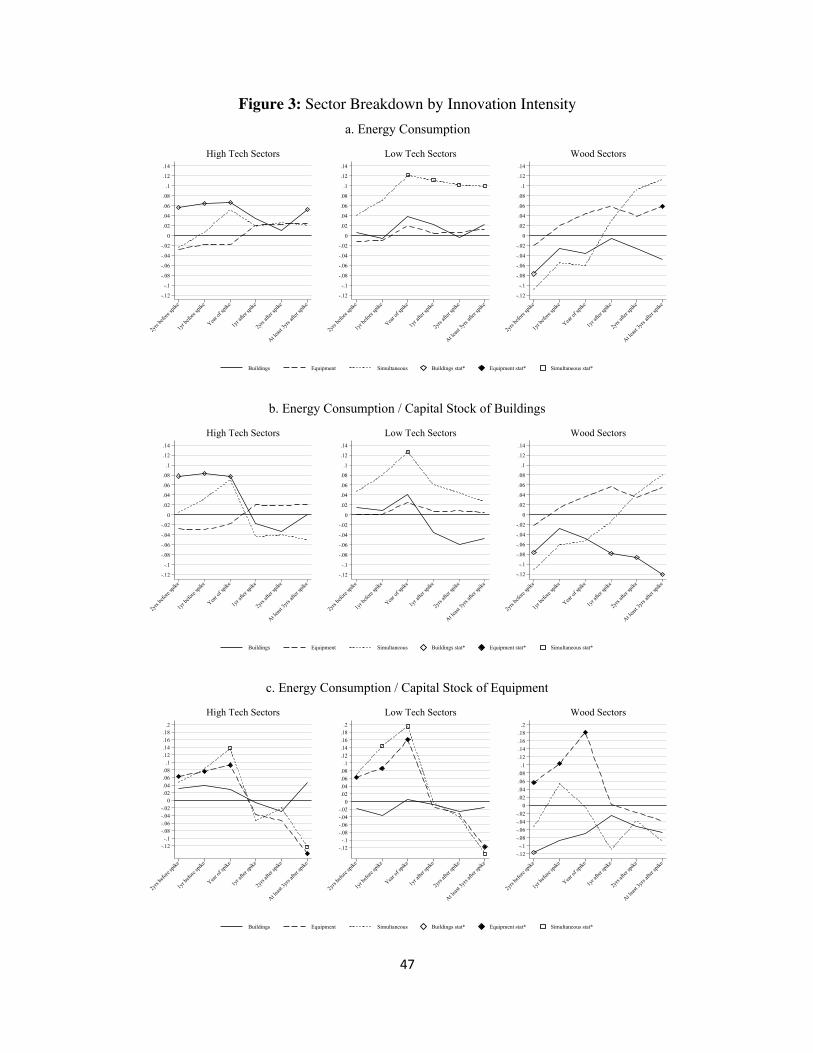
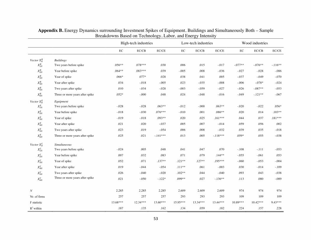
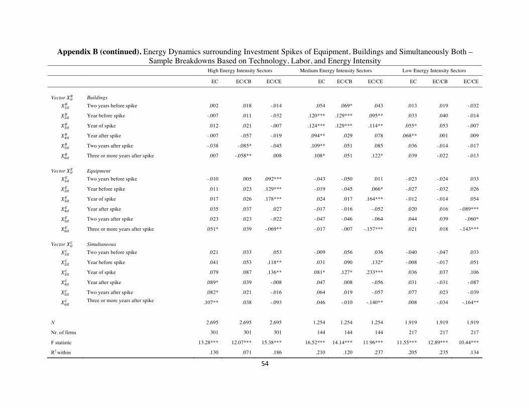
The table in Appendix B presents the results of our analysis conducted on sample breakdowns by

innovation, labor and energy intensity to obtain a more granular insight. Based on these results, we

constructed Figures 3 to 5. In Figure 3 we depict the results distinguishing firms by innovation

intensity. In this discussion we disregard the separate Wood sectors as these yield few statistically

significant results in terms of what happens after the various spike events. We see from Figure 3

that our findings for the full sample are largely in line with those for the Low Tech sectors. In these

sectors energy usage increases substantially by approximately 10 percent after a simultaneous

spike. According to the table in Appendix B energy efficiency improves three or more years after

investing in equipment (single or simultaneous spike). Firms in High Tech sectors do also improve

energy efficiency when investing in equipment (single or simultaneous spike). This does increase

overall usage of energy significantly by about 5 percent after three or more years, but this number

is substantially lower than what we observe for the Low Tech sectors.

*** Figure 3 about here ***

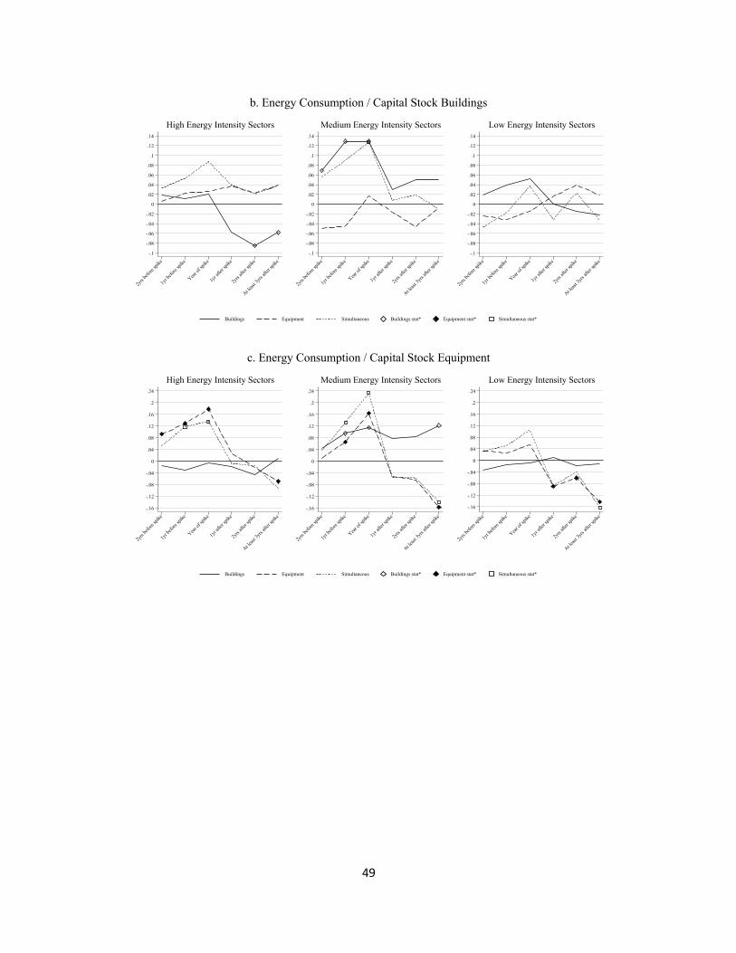
In Figure 4 we present our results distinguishing firms by energy intensity. We observe that

similar to our results based on the full sample, energy efficiency improves when investing in

equipment (single and simultaneous spike) in essentially all sectors. Only in High Energy Intensity

sectors a simultaneous spike does not yield a statistically significant result for three or more years

after the spike, though the sign and size of the coefficient are in the right direction. However, we

see that in High Energy Intensity sectors after a simultaneous spike energy usage increases

afterwards. In Medium and Low Energy Intensity sectors we do not observe this pattern. Instead

32

in Medium Energy Intensity sectors it is major investments in buildings that are associated with

higher energy usage.

*** Figure 4 about here ***

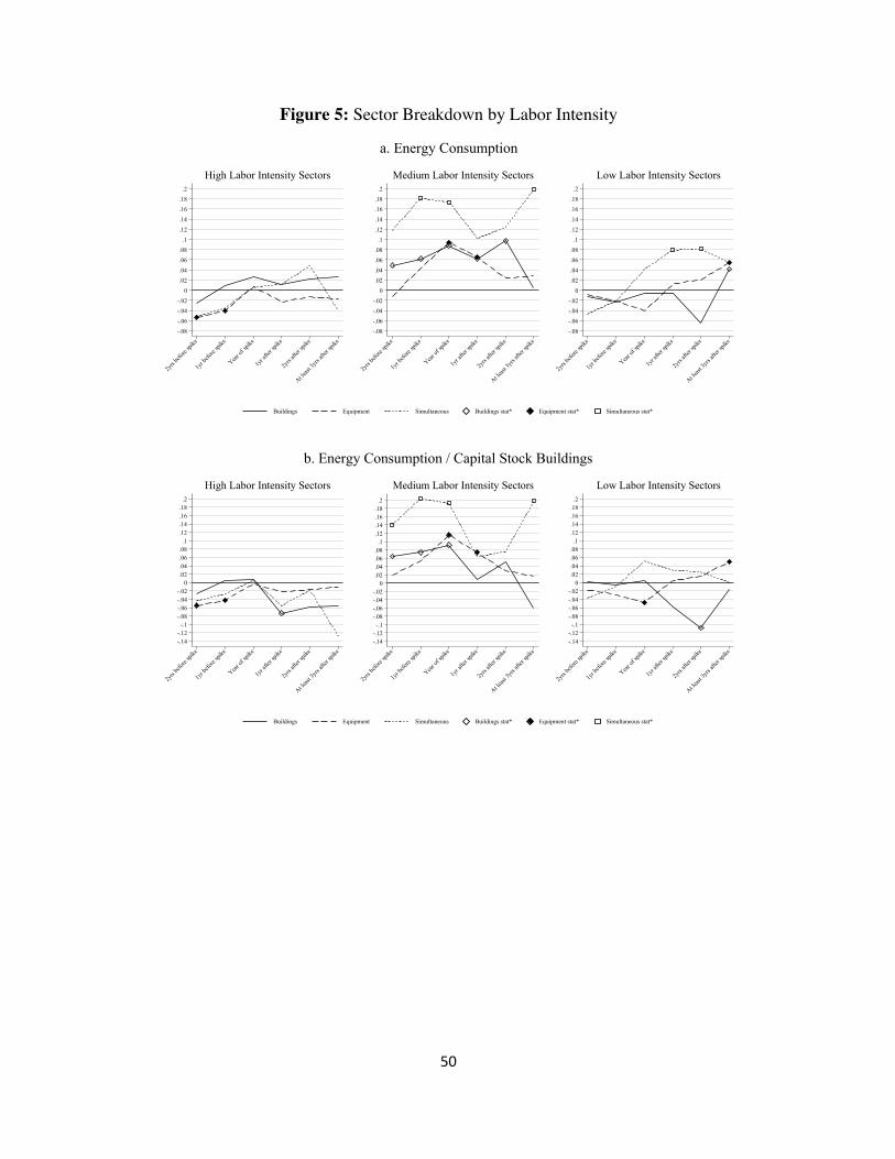
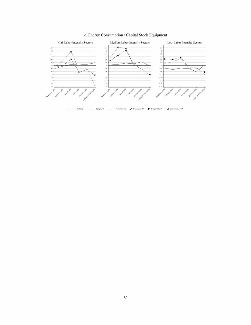
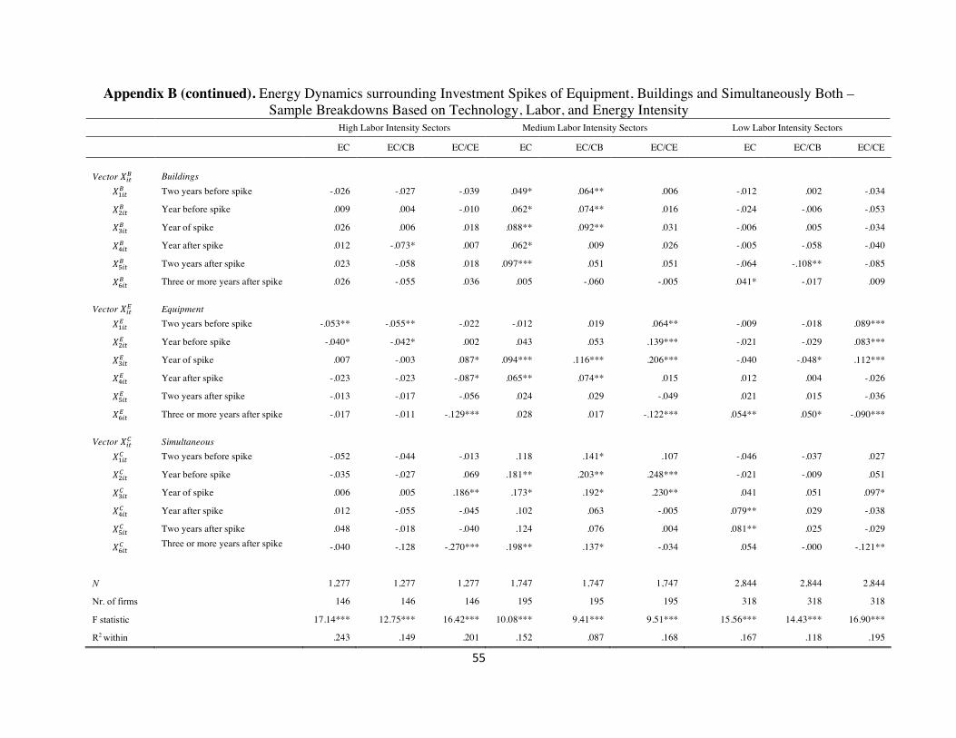
In Figure 5 we depict our results breaking down sectors by labor intensity. We see that energy

efficiency improves three or more years after investing in equipment (single and simultaneous

spike) except for the Medium Labor Intensity sectors where those improvements are not visible

after simultaneous spikes. Nevertheless, in Medium Labor Intensity sectors we do observe an

increase in energy usage three or more years afterwards. Strikingly, we find that in Low Labor

Intensive sectors after single spikes in buildings and equipment energy usage expands.

*** Figure 5 about here ***

In sum, we find some differences across various types of industries as distinguished by

innovation, energy and labor intensity. However, the result that major investments involving

equipment (single and simultaneous spikes) are correlated with better energy efficiency is largely

robust across sectors. The result that simultaneous spikes are associated with higher energy usage

is found most strongly in Low Tech, High Energy Intensity and Medium Labor Intensity sectors.

Operational Efficiency

In Table 6 we report how efficiency of the firm evolves surrounding major investment events for

the full sample, as well as for the sample breakdowns by technology, labor, and energy intensity.

In case of simultaneous spikes, we observe that the total cost to sales ratio does not change

significantly. Operational efficiency tends to improve three or more years after an investment spike

33

in equipment only, though investments in buildings do the opposite. In the full sample efficiency

does not get worse by more than 1 percent.

34

Table 6 Economic Performance surrounding Investment Spikes of Equipment, Buildings and Simultaneously Both

TC/S

Full Sample HT W LT HE ME LE HL ML LL

Vector !"#$ Buildings

!%"#$ Two years before spike -.005 .001 -.013 -.006 .005 -.016 -.016** -.026*** -.022** .013

!&"#$ Year before spike -.007 -.007 -.012* -.005 -.001 -.003 -.017** -.011 -.016* .004

!'"#$ Year of spike -.004 -.004 .003 -.010 .001 .004 -.016* -.005 -.015 .006

!("#$ Year after spike .005 .004 .020** -.004 .007 .007 .000 .008 -.004 .011

!)"#$ Two years after spike .003 .005 .014 -.006 .004 -.000 .003 .009 -.002 .005

!*"#$ Three or more years after spike .010** .017* .003 .002 .016** .002 .004 -.003 .003 .019***

Vector !"#+ Equipment

!%"#+ Two years before spike -.004 -.014 -.021** .012* .005 .012 -.028*** .010 -.014 -.007

!&"#+ Year before spike -.011** -.020** -.018** .000 -.002 -.006 -.026*** .001 -.015* -.013*

!'"#+ Year of spike .002 -.006 -.008 .012 .010 .008 -.015 .010 .001 -.002

!("#+ Year after spike .009* .004 .009 .013* .018** -.003 .002 -.006 .022** .007

!)"#+ Two years after spike .014** .017 .009 .013** .013** .013 .016 .019* .026* .006

!*"#+ Three or more years after spike -.008* -.026*** .005 -.000 .003 -.018** -.022** -.017* -.012 -.004

Vector !"#, Simultaneous

!%"#, Two years before spike -.027 -.024 -.017* -.032 -.034 -.028 -.011 .017 -.045* -.030

!&"#, Year before spike -.008 -.013 -.031* .004 .002 -.020 -.020 -.004 -.051** .010

!'"#, Year of spike .002 -.003 -.016 .014 .007 -.011 .004 .019 -.038 .014

!("#, Year after spike .007 -.001 -.009 .017 .015 -.013 .005 .003 -.008 .014

!)"#, Two years after spike .013 .001 .023 .018* .017 -.007 .017 .019 -.013 .021**

!*"#, Three or more years after spike -.000 -.028 .000 .017 .008 -.011 -.023 .011 -.022 .006

N 5,868 2,285 974 2,609 2,695 1,254 1,919 1,277 1,747 2,844

Nr. of firms 652 257 109 293 301 144 217 146 195 318

F statistic 2.89*** 2.07*** 2.04*** 1.69** 2.24*** 1.97*** 2.33*** 2.16*** 2.41*** 2.01***

R2 within .016 .025 .052 .025 .018 .029 .041 .039 .041 .017

35

Notes: Table 6 presents the results of the estimation parameters for the economic performance surrounding investment spikes in equipment, buildings and simultaneously both. The dependent variable across regressions is on the horizontal row and has received a (natural) logarithmic transformation. Dependent variable: TC/S = Total Costs / Sales. Abbreviations: HT (LT) = High- (Low-) tech industries, W = Wood, HE (ME, LE) = High (Medium, Low) energy intensity industries, HL, (ML, LL) = High (Medium, Low) labor intensity industries. Parameter estimates, conditioned upon observing an investment spike, are documented by investment spike time and investment type. The models include year dummies, but omitted from table display. Statistical significance is reflected by: * p ≤ .10, ** p ≤ .05, *** p ≤ .01.

36

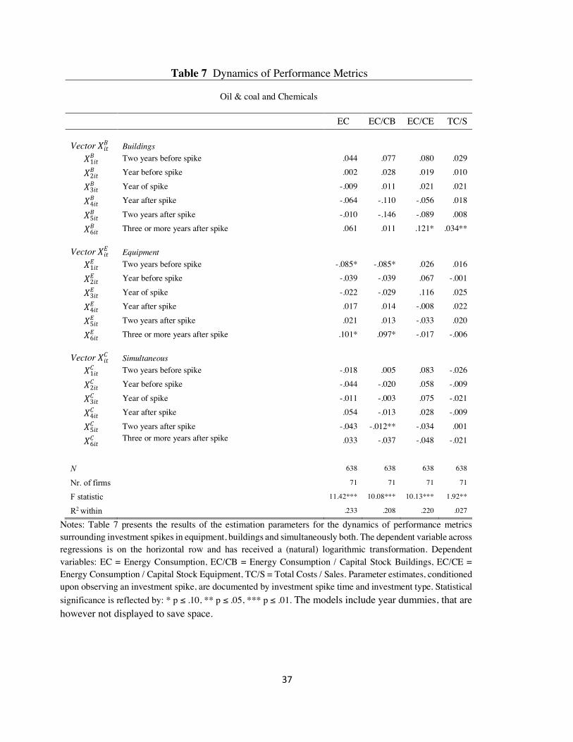
Operational Efficiency in Oil & coal and Chemicals

According to Table 6 sectors that are harmed most in terms of operational efficiency by investment

in buildings are high-tech industries, industries with low labor intensity and those with high energy

intensity. With these categories in mind, Table 3 informs firms operating in Oil & coal and in

Chemicals face a statistically significant financial disincentive to invest in buildings. Operational

efficiency decreases by more than 1.5 percentage points in such capital-intensive industries. This

is confirmed by a separate analysis reported in Table 7 that we conducted for these sectors.

Operational efficiency decreases by 3.4 percent after three or more years after a spike in buildings

when we group the observations for Oil & coal and Chemicals. This result is statistically

significant. For these sectors we find that upon investment, energy use does increase, however only

a single investment spike in equipment does so according to conventional statistical significance

levels. Likewise, previous literature identified that in Chemicals firms increased energy

consumption after participating in voluntary energy efficiency equipment programs (Gamper-

Rabindran and Finger, 2013). Nevertheless, our results suggest that also in these industries

implying that investment is associated with higher energy efficiency. We conclude that

the sectors mentioned in this paragraph may enhance environmental performance by investing in

appropriate capital goods. Nevertheless, appropriate financial incentives to do so seem absent.

ln 0kD >

37

Table 7 Dynamics of Performance Metrics

Oil & coal and Chemicals

EC EC/CB EC/CE TC/S

Vector !"#$ Buildings

!1"#$ Two years before spike .044 .077 .080 .029

!2"#$ Year before spike .002 .028 .019 .010

!3"#$ Year of spike -.009 .011 .021 .021

!4"#$ Year after spike -.064 -.110 -.056 .018

!5"#$ Two years after spike -.010 -.146 -.089 .008

!6"#$ Three or more years after spike .061 .011 .121* .034**

Vector !"#+ Equipment

!1"#+ Two years before spike -.085* -.085* .026 .016

!2"#+ Year before spike -.039 -.039 .067 -.001

!3"#+ Year of spike -.022 -.029 .116 .025

!4"#+ Year after spike .017 .014 -.008 .022

!5"#+ Two years after spike .021 .013 -.033 .020

!6"#+ Three or more years after spike .101* .097* -.017 -.006

Vector !"#, Simultaneous

!1"#, Two years before spike -.018 .005 .083 -.026

!2"#, Year before spike -.044 -.020 .058 -.009

!3"#, Year of spike -.011 -.003 .075 -.021

!4"#, Year after spike .054 -.013 .028 -.009

!5"#, Two years after spike -.043 -.012** -.034 .001

!6"#, Three or more years after spike .033 -.037 -.048 -.021

N 638 638 638 638

Nr. of firms 71 71 71 71

F statistic 11.42*** 10.08*** 10.13*** 1.92**

R2 within .233 .208 .220 .027

Notes: Table 7 presents the results of the estimation parameters for the dynamics of performance metrics surrounding investment spikes in equipment, buildings and simultaneously both. The dependent variable across regressions is on the horizontal row and has received a (natural) logarithmic transformation. Dependent variables: EC = Energy Consumption, EC/CB = Energy Consumption / Capital Stock Buildings, EC/CE = Energy Consumption / Capital Stock Equipment, TC/S = Total Costs / Sales. Parameter estimates, conditioned upon observing an investment spike, are documented by investment spike time and investment type. Statistical significance is reflected by: * p ≤ .10, ** p ≤ .05, *** p ≤ .01. The models include year dummies, that are however not displayed to save space.

38

6. Conclusion

Environmental performance is a core 21st century challenge and firms have an important role to

play in increasing energy efficiency and decreasing toxic pollutants. Yet, there is limited evidence

on the links between firm investment activities and how they can be used to change environmental

performance outcomes. For firms, investment events are where they can plan for financial and

environmental performance. Large investment spikes influence the productivity of firms, can

impact hundreds of employees, change operational costs and influence the production of millions

of manufactured goods. Hence, firms seek efficiency in equipment, buildings or the simultaneous

use of both. We investigate how energy performance of Dutch manufacturing firms over the 2000

to 2008 period evolves in the time surrounding investment spikes in capital. Our contribution is to

identify whether these investment spikes had an impact on energy consumption, assess whether or

not firms improved energy efficiency in anticipation of the investment event or after an investment

outlay occurred and identify the capital source where environmental performance is correlated with

investment spikes.

From our multi-period event study, we find that when firms engage in large simultaneous

investments in both buildings and equipment, energy consumption levels increase considerably by

6.4 percent in the first year after the spike and continues to rise to an average 7.4 percent in 3 or

more years. For this result, we may be able to interpret a simultaneous capital expenditure as a

signal of expansionary or replacement activities and potentially implies that when firms engage in

growth activities there is correlation with energy consumption growth overall. This result correlates

with expectations around firm investment, but it does not necessarily point to poor environmental

performance from the building or equipment capital. In fact, we find that in cases of major

investment spikes energy efficiency improves. Moreover, we find that these investments do not

39

correlate with an increase in the total cost per sales after an investment is made. Notably,

investments in equipment improve the operational efficiency by approximately 2 percent after three

years from the investment spike. This suggests that industrial firms can decrease energy

consumption whilst increasing operational efficiency – the so called “doing well by doing good”.

We find that after investments energy efficiency in equipment improves. Our results for the

overall sample imply that less energy is needed to produce a certain level of output once a firm

invests. We show that after three years from the investment outlay energy efficiency increases by

about 12 percent per unit of equipment. Though energy efficiency improves after installing new

equipment capital, we observe some evidence of energy efficiency decreasing subsequent to

investment in buildings in high technology, high energy and low labor industries by 1.7, 1.6 and

1.9 percent respectively. Especially firms operating in capital-intensive industries like Oil & Coal

and Chemicals seem to be affected by stricter building codes.

Our results document a positive correlation with environmental performance after

investment spike activity, which suggests firms investing in industrial buildings do so with energy

efficiency as a primary objective for financial performance. Anecdotally, there is evidence of

success in the industrial sector to meet energy efficiency performance targets. As an example,

Prologis is a global industrial real estate company that is committed to decreased energy

consumption to improve financial performance.8 However, from a policy perspective lagged firm

awareness, poor environmental performance knowledge on behalf of firms, poor equipment and(or)

8 Prologis is a large industrial real estate investment trust operating in North America, Europe and Asia. They were recently acknowledged by the Green Real Estate Sustainability Benchmark for their ten years of superior energy consumption in the sector. See also https://www.prologis.com/logistics-industry-feature/prologis-earns-perfect-10-2017-sustainability-benchmark, accessed 08/28/2018.

40

building standards knowledge or lagged policy implementation may lead to decreased planning for

environmental performance at the time of investment spikes. Thus, more common policy

approaches like voluntary agreements with firms may not be of much help in this context, but third-

party verification or enforceable penalties when firms do not perform, subsidies or R&D tax credits

could potentially yield better results (Earnhart, 2004; Cole et al., 2005; Gamper-Rabindran and

Finger, 2013).

Currently, CBS data does not enable us to identify the effect of energy efficiency standards

or codes in our results and more generally there are limitations around observing expansionary

events by firms. In addition, we do not observe substitution of activities between plants that belong

to the same company. Future research may also seek to observe expansionary investment in BRIC

economies. However, our results have allowed us to observe that there is a correlation between

energy related metrics and firms who have purchased new equipment capital. For policy makers to

take note, we observe that growing firms become more energy efficient. Firms conducting large

investments are planning for a future cash flow that is promising and invest in equipment where

they expect to yield a profit maximizing positive financial return from such decisions. Furthermore,

it is financially healthy firms having cash flow streams and/or access to the capital markets that are

capable of investments at this magnitude. Sometimes firms need to finance capital improvement

expenditures themselves due to capital market imperfections (Fazzari et al., 1988), but in the EU’s

current Horizon 2020 program there are numerous avenues to apply for financing and subsidies

that support the purchase of new energy efficient equipment and building technologies. Potentially

in the long-run, as the manufacturing sector switches towards environmental performing capital,

then energy efficient firm production could replace firm production that is both less successful and

energy inefficient. In the aggregate, technological progress in equipment and buildings both with

41

an aim towards energy efficiency may be improved by replacement of unsuccessful firms by more

energy efficient competitors (Acemoglu et al., 2014; Acemoglu et al., 2009).

In this way, policy makers should continue to recognize, convene and set standards towards

industrial environmental performance. Environmental goals can be attained by advancing standards

for materials, equipment, building codes and the emissions of pollutants without significant

financial repercussions to firms. This view is consistent with studies observing that “lean and

green” go hand in hand. Investing in environmental technology enhances manufacturing

performance (Klassen and Wybark, 1999; Telle and Larsson, 2007) and lean production processes

are complementary to environmental performance (King and Lenox, 2001). Future research is

required to understand whether it is such evolutionary developments in industries, allowing

countries to become less dependent on energy in the aggregate.

42

References

Abel, A.B. and Eberly, J.C. (1994). A unified model of investment under uncertainty. American Economic Review, 84, 1369-1384.

Abel, A.B., and Eberly, J.C. (1998). The mix and scale of factors with irreversibility and fixed costs of investment. Carnegie Rochester Conference Series on Public Policy, 48, 101-135. Acemoglu, D. (2015). How the machines replace labor? Paper presented at the annual meeting of the Allied Social Science Associations, American Economic Association, Boston.

Acemoglu, D., Aghion, P., Bursztyn, L., and Hemous, D. (2009). The environment and directed technical change (No. w15451). National Bureau of Economic Research. Acemoglu, D., Akcigit, U., Hanley, D. and Kerr, W. (2014). Transition to clean technology (No. w20743). National Bureau of Economic Research. Aroonruengsawat, A., Auffhammer, M., and Sanstad, A. H. (2012). The impact of state level building codes on residential electricity consumption. Energy Journal-Cleveland, 33, 31. Asphjell, M.K., Letterie, W., Nilsen, Ø.A. and Pfann, G.A. (2014). Sequentiality versus simultaneity: Interrelated factor demand. Review of Economics and Statistics, 96, 986-998. van den Bergen, D., de Haan, M., de Hey, R. and Horsten, M. (2009). Measuring capital in the Netherlands. Statistics Netherlands Discussion Paper (09036). Bokhari, S. & Geltner, D. (2014). Characteristics in commercial and multi-family property: An investment perspective. Center for Real Estate Working Paper Series. Bloom, N. (2009). The impact of uncertainty shocks. Econometrica, 77, 623-685. Chegut, A., Eichholtz, P.M., and Rodrigues, J.M. (2014). Spatial dependence in international office markets. Journal of Real Estate Finance and Economics, 51, 317-350. Cole, M.A., Elliott, R.J. and Shimamoto, K., (2005). Industrial characteristics, environmental regulations and air pollution: an analysis of the UK manufacturing sector. Journal of Environmental Economics and Management, 50 (1), 121-143. Cooper, R. W., & Haltiwanger, J. C. (2006). On the nature of capital adjustment costs. The Review of Economic Studies, 73(3), 611-633.

Cooper, R.W., Haltiwanger, J.C. and Power, L.(1999). Machine Replacement and Business Cycle: Lumps and Bumps. American Economic Review. 89(4), 921-946.

43

Dalton, B., and Fuerst, F. (2018). The ‘green value’proposition in real estate. Routledge Handbook of Sustainable Real Estate. Dunne, T., Roberts, M.J. and Samuelson, L. (1989). Firm turnover and gross employment flows in the US manufacturing sector. Journal of Labor Economics, 7, 48-71. Earnhart, D., (2004). Regulatory factors shaping environmental performance at publicly-owned treatment plants. Journal of Environmental Economics and Management, 48(1), pp.655-681. Eichholtz, P., Kok, N., and Quigley, J. M. (2010). Doing well by doing good? Green office buildings. American Economic Review, 100(5), pp.2492-2509. European Environment Agency. (2013). Final energy consumption by sector (CSI 027/ENER 016). http://www.eea.europa.eu/data-and-maps/indicators/final-energy-consumption-by-sector-5/assessment. Accessed July 9, 2014. Gamper-Rabindran, S. and Finger, S.R., (2013). Does industry self-regulation reduce pollution? Responsible Care in the chemical industry. Journal of Regulatory Economics, 43(1), pp.1-30. Görzig, B., (2007). Depreciation in EU member states: empirical and methodological differences. EU KLEMS Project. Hamermsh, D, and Pfann, G. (1996). Adjustment costs in factor demand. Journal of Economic Literature, 34, 1264-1292. Hémous, D., and Olsen, M. (2013). The rise of the machines: automation, horizontal innovation and income inequality. Paper presented at the annual meeting of the Allied Social Science Associations, American Economic Association, Boston. International Energy Agency (2014). Energy Policies of IEA countries. The Netherlands. 2014 Review. OECD/IEA. Jacobsen, G.J. and Kotchen, M.J. (2013). Are building codes effective at saving energy? Evidence from residential billing data in Florida. Review of Economics and Statistics, 95, 34-49. Kapelko, M., Oude Lansink, A. and Stefanou, S.E. (2015) Analyzing the impact of investment spikes on dynamic productivity growth. Omega, 54, 116-124. King, A.A. and Lenox, M.J., (2001). Lean and green? An empirical examination of the relationship between lean production and environmental performance. Production and Operations Management, 10(3), pp.244-256. Klassen, R.D. and Whybark, D.C., (1999). The impact of environmental technologies on manufacturing performance. Academy of Management Journal, 42(6), pp.599-615.

44

Letterie, W.A., and Pfann, G.A. (2007). Structural identification of high and low investment regimes. Journal of Monetary Economics, 54, 797-819. Letterie, W., Pfann, G. A., and Verick, S. (2010). On lumpiness in the replacement and expansion of capital. Oxford Bulletin of Economics and Statistics, 72(3), 263-281 Letterie, W., Pfann, G.A. and Polder, J.M. (2004). Factor adjustment spikes and interrelation: An empirical investigation. Economics Letters, 85, 145-150. Nilsen, Ø. A., Raknerud, A., Rybalka, M., & Skjerpen, T. (2009). Lumpy investments, factor adjustments, and labor productivity. Oxford Economic Papers, 61, 104-127. Nilsen, Ø .A. and Schiantarelli, F. (2003). Zeros and lumps in investment: Empirical evidence on irriversibilities and nonconvexities, Review of Economics & Statistics, 85(4), 1021-1037. Papineau, Maya. (2013). Energy codes and the landlord-tenant Problem. UC Berkeley: Fisher Center for Real Estate and Urban Economics. Retrieved from: https://escholarship.org/uc/item/46c518h9 Power, L. (1998). The missing link: technology, investment, and productivity. Review of Economics and Statistics, 80, 300-313. Ramirez, C.A., Patel, M. and Blok, K. (2005). The non-energy intensive manufacturing sector. An energy analysis relating to the Netherlands. Energy, 30, 749-767. Raymond, W., Mohnen, P., Palm, F. & Schim van der Loeff, S. (2006). A classification of Dutch manufacturing based on a model of innovation. De Economist, 154, 85-105. Sakellaris, P. (2004). Patterns of firm adjustment. Journal of Monetary Economics, 51, 425-450. Telle, K. and Larsson, J., (2007). Do environmental regulations hamper productivity growth? How accounting for improvements of plants' environmental performance can change the conclusion. Ecological Economics, 61(2), pp.438-445. Verdolini, E. and Galeotti, M., (2011). At home and abroad: An empirical analysis of innovation and diffusion in energy technologies. Journal of Environmental Economics and Management, 61(2), 119-134. Wooldridge, J. M. (2013). Introductory Econometrics–A Modern Approach, 5th edition. Boston, MA: Cengage Learning. US Energy Information Administration. (2014). AEO2014 Early Release Overview. Report Number DOE/EIA 0383ER(2014).

45

Figures

Figure 1: Energy Consumption

-.02

-.01

0

.01

.02

.03

.04

.05

.06

.07

.08

2yrs

befor

e spik

e

1yr b

efore

spike

Year o

f spik

e

1yr a

fter s

pike

2yrs

after

spike

At least

3yrs

after

spike

Buildings Equipment Simultaneous Buildings stat* Equipment stat* Simultaneous stat*

Energy Consumption

46

Figure 2: Energy Efficiency of Buildings and Equipment

-.14

-.12

-.1

-.08

-.06

-.04

-.02

0

.02

.04

.06

.08

.1

.12

.14

2yrs

befor

e spik

e

1yr b

efore

spike

Year o

f spik

e

1yr a

fter s

pike

2yrs

after

spike

At least

3yrs

after

spike

Energy Consumption / Cap. St. Buildings

-.14

-.12

-.1

-.08

-.06

-.04

-.02

0

.02

.04

.06

.08

.1

.12

.14

2yrs

befor

e spik

e

1yr b

efore

spike

Year o

f spik

e

1yr a

fter s

pike

2yrs

after

spike

At least

3yrs

after

spike

Energy Consumption / Cap. St. Equipment

Buildings Equipment Simultaneous Buildings stat* Equipment stat* Simultaneous stat*

47

Figure 3: Sector Breakdown by Innovation Intensity

-.12

-.1

-.08

-.06

-.04

-.02

0

.02

.04

.06

.08

.1

.12

.14

2yrs

befor

e spik

e

1yr b

efore

spike

Year of

spike

1yr a

fter s

pike

2yrs

after

spike

At least

3yrs

after

spike

High Tech Sectors

-.12

-.1

-.08

-.06

-.04

-.02

0

.02

.04

.06

.08

.1

.12

.14

2yrs

befor

e spik

e

1yr b

efore

spike

Year of

spike

1yr a

fter s

pike

2yrs

after

spike

At least

3yrs

after

spike

Low Tech Sectors

-.12

-.1

-.08

-.06

-.04

-.02

0

.02

.04

.06

.08

.1

.12

.14

2yrs

befor

e spik

e

1yr b

efore

spike

Year of

spike

1yr a

fter s

pike

2yrs

after

spike

At least

3yrs

after

spike

Wood Sectors

a. Energy Consumption

Buildings Equipment Simultaneous Buildings stat* Equipment stat* Simultaneous stat*

-.12

-.1

-.08

-.06

-.04

-.02

0

.02

.04

.06

.08

.1

.12

.14

2yrs

befor

e spik

e

1yr b

efore

spike

Year of

spike

1yr a

fter s

pike

2yrs

after

spike

At least

3yrs

after

spike

High Tech Sectors

-.12

-.1

-.08

-.06

-.04

-.02

0

.02

.04

.06

.08

.1

.12

.14

2yrs

befor

e spik

e

1yr b

efore

spike

Year of

spike

1yr a

fter s

pike

2yrs

after

spike

At least

3yrs

after

spike

Low Tech Sectors

-.12

-.1

-.08

-.06

-.04

-.02

0

.02

.04

.06

.08

.1

.12

.14

2yrs

befor

e spik

e

1yr b

efore

spike

Year of

spike

1yr a

fter s

pike

2yrs

after

spike

At least

3yrs

after

spike

Wood Sectors

b. Energy Consumption / Capital Stock of Buildings

Buildings Equipment Simultaneous Buildings stat* Equipment stat* Simultaneous stat*

-.12-.1

-.08-.06-.04-.02

0.02.04.06.08

.1.12.14.16.18

.2

2yrs

befor

e spik

e

1yr b

efore

spike

Year of

spike

1yr a

fter s

pike

2yrs

after

spike

At least

3yrs

after

spike

High Tech Sectors

-.12-.1

-.08-.06-.04-.02

0.02.04.06.08.1

.12

.14

.16

.18.2

2yrs

befor

e spik

e

1yr b

efore

spike

Year of

spike

1yr a

fter s

pike

2yrs

after

spike

At least

3yrs

after

spike

Low Tech Sectors

-.12-.1

-.08-.06-.04-.02

0.02.04.06.08

.1.12.14.16.18

.2

2yrs

befor

e spik

e

1yr b

efore

spike

Year of

spike

1yr a

fter s

pike

2yrs

after

spike

At least

3yrs

after

spike

Wood Sectors

c. Energy Consumption / Capital Stock of Equipment

Buildings Equipment Simultaneous Buildings stat* Equipment stat* Simultaneous stat*

48

Figure 4: Sector Breakdown by Energy Intensity

-.06

-.04

-.02

0

.02

.04

.06

.08

.1

.12

.14

2yrs

befor

e spik

e

1yr b

efore

spike

Year of

spike

1yr a

fter s

pike

2yrs

after

spike

At least

3yrs

after

spike

High Energy Intensity Sectors

-.06

-.04

-.02

0

.02

.04

.06

.08

.1

.12

.14

2yrs

befor

e spik

e

1yr b

efore

spike

Year of

spike

1yr a

fter s

pike

2yrs

after

spike

At least

3yrs

after

spike

Medium Energy Intensity Sectors

-.06

-.04

-.02

0

.02

.04

.06

.08

.1

.12

.14

2yrs

befor

e spik

e

1yr b

efore

spike

Year of

spike

1yr a

fter s

pike

2yrs

after

spike

At least

3yrs

after

spike

Low Energy Intensity Sectors

a. Energy Consumption

Buildings Equipment Simultaneous Buildings stat* Equipment stat* Simultaneous stat*

49

-.1

-.08

-.06

-.04

-.02

0

.02

.04

.06

.08

.1

.12

.14

2yrs

befor

e spik

e

1yr b

efore

spike

Year of

spike

1yr a

fter s

pike

2yrs

after

spike

At least

3yrs

after

spike

High Energy Intensity Sectors

-.1

-.08

-.06

-.04

-.02

0

.02

.04

.06

.08

.1

.12

.14

2yrs

befor

e spik

e

1yr b

efore

spike

Year of

spike

1yr a

fter s

pike

2yrs

after

spike

At least

3yrs

after

spike

Medium Energy Intensity Sectors

-.1

-.08

-.06

-.04

-.02

0

.02

.04

.06

.08

.1

.12

.14

2yrs

befor

e spik

e

1yr b

efore

spike

Year of

spike

1yr a

fter s

pike

2yrs

after

spike

At least

3yrs

after

spike

Low Energy Intensity Sectors

b. Energy Consumption / Capital Stock Buildings

Buildings Equipment Simultaneous Buildings stat* Equipment stat* Simultaneous stat*

-.16

-.12

-.08

-.04

0

.04

.08

.12

.16

.2

.24

2yrs

befor

e spik

e

1yr b

efore

spike

Year of

spike

1yr a

fter s

pike

2yrs

after

spike

At least

3yrs

after

spike

High Energy Intensity Sectors

-.16

-.12

-.08

-.04

0

.04

.08

.12

.16

.2

.24

2yrs

befor

e spik

e

1yr b

efore

spike

Year of

spike

1yr a

fter s

pike

2yrs

after

spike

At least

3yrs

after

spike

Medium Energy Intensity Sectors

-.16

-.12

-.08

-.04

0

.04

.08

.12

.16

.2

.24

2yrs

befor

e spik

e

1yr b

efore

spike

Year of

spike

1yr a

fter s

pike

2yrs

after

spike

At least

3yrs

after

spike

Low Energy Intensity Sectors

c. Energy Consumption / Capital Stock Equipment

Buildings Equipment Simultaneous Buildings stat* Equipment stat* Simultaneous stat*

50

Figure 5: Sector Breakdown by Labor Intensity

-.08

-.06

-.04

-.02

0

.02

.04

.06

.08

.1

.12

.14

.16

.18

.2

2yrs

befor

e spik

e

1yr b

efore

spike

Year of

spike

1yr a

fter s

pike

2yrs

after

spike

At least

3yrs

after

spike

High Labor Intensity Sectors

-.08

-.06

-.04

-.02

0

.02

.04

.06

.08

.1

.12

.14

.16

.18

.2

2yrs

befor

e spik

e

1yr b

efore

spike

Year of

spike

1yr a

fter s

pike

2yrs

after

spike

At least

3yrs

after

spike

Medium Labor Intensity Sectors

-.08

-.06

-.04

-.02

0

.02

.04

.06

.08

.1

.12

.14

.16

.18

.2

2yrs

befor

e spik

e

1yr b

efore

spike

Year of

spike

1yr a

fter s

pike

2yrs

after

spike

At least

3yrs

after

spike

Low Labor Intensity Sectors

a. Energy Consumption

Buildings Equipment Simultaneous Buildings stat* Equipment stat* Simultaneous stat*

-.14-.12

-.1-.08-.06-.04-.02

0.02.04.06.08

.1.12.14.16.18

.2

2yrs

befor

e spik

e

1yr b

efore

spike

Year of

spike

1yr a

fter s

pike

2yrs

after

spike

At least

3yrs

after

spike

High Labor Intensity Sectors

-.14-.12

-.1-.08-.06-.04-.02

0.02.04.06.08.1

.12

.14

.16

.18.2

2yrs

befor

e spik

e

1yr b

efore

spike

Year of

spike

1yr a

fter s

pike

2yrs

after

spike

At least

3yrs

after

spike

Medium Labor Intensity Sectors

-.14-.12

-.1-.08-.06-.04-.02

0.02.04.06.08

.1.12.14.16.18

.2

2yrs

befor

e spik

e

1yr b

efore

spike

Year of

spike

1yr a

fter s

pike

2yrs

after

spike

At least

3yrs

after

spike

Low Labor Intensity Sectors

b. Energy Consumption / Capital Stock Buildings

Buildings Equipment Simultaneous Buildings stat* Equipment stat* Simultaneous stat*

51

-.28

-.24

-.2

-.16

-.12

-.08

-.04

0

.04

.08

.12

.16

.2

.24

2yrs

befor

e spik

e

1yr b

efore

spike

Year of

spike

1yr a

fter s

pike

2yrs

after

spike

At least

3yrs

after

spike

High Labor Intensity Sectors

-.28

-.24

-.2

-.16

-.12

-.08

-.04

0

.04

.08

.12

.16

.2

.24

2yrs

befor

e spik

e

1yr b

efore

spike

Year of

spike

1yr a

fter s

pike

2yrs

after

spike

At least

3yrs

after

spike

Medium Labor Intensity Sectors

-.28

-.24

-.2

-.16

-.12

-.08

-.04

0

.04

.08

.12

.16

.2

.24

2yrs

befor

e spik

e

1yr b

efore

spike

Year of

spike

1yr a

fter s

pike

2yrs

after

spike

At least

3yrs

after

spike

Low Labor Intensity Sectors

c. Energy Consumption / Capital Stock Equipment

Buildings Equipment Simultaneous Buildings stat* Equipment stat* Simultaneous stat*

52

Appendix A. Construction of Capital Stock Variables

We construct the starting value of a firm’s capital stock for buildings and for equipment as follows.

The initial capital stock for a firm is the contemporaneous ratio of firm to industry output multiplied

by the industry’s capital stock of an asset. More specifically, for a given firm i in period t, the firm’s

capital stock, i.e. is calculated using , where j denotes the industry a firm is

operating in, ( ) depicts output of firm i (industry j) in year t, ( ) denotes the capital

stock of asset c of company i (industry j) at the beginning of year t. The industry level data are

obtained from the Statline online data center of Statistics Netherlands (CBS). To construct the

starting values of the capital stock series, data from the year prior to the start of the sample are

collected. Hence, these series start in the year 2000.

The capital stock for the remaining years is determined by the perpetual inventory method.

Importantly, in the analysis we employ real investment and capital figures. The nominal numbers

have been deflated using producer price indices on buildings or equipment assets. The nominal

numbers refer to investments done in the book year.

citK

c c itit jt

jt

YK KY

= ×

itY jtYcitK

cjtK

53

Appendix B. Energy Dynamics surrounding Investment Spikes of Equipment, Buildings and Simultaneously Both – Sample Breakdowns Based on Technology, Labor, and Energy Intensity

High-tech industries Low-tech industries Wood industries

EC EC/CB EC/CE EC EC/CB EC/CE EC EC/CB EC/CE

Vector !"#$ Buildings

!%"#$ Two years before spike .056** .078*** .030 .006 .015 -.017 -.077** -.076** -.116**

!&"#$ Year before spike .064** .083*** .039 -.005 .008 -.036 -.027 -.028 -.086

!'"#$ Year of spike .066* .077* .028 .038 .041 .005 -.037 -.049 -.070

!("#$ Year after spike .034 -.018 -.005 .023 -.035 -.008 -.006 -.078* -.024

!)"#$ Two years after spike .010 -.034 -.028 -.003 -.059 -.027 -.026 -.087** -.053

!*"#$ Three or more years after spike .052* -.000 .048 .024 -.048 -.016 -.049 -.121** -.067

Vector !"#+ Equipment

!%"#+ Two years before spike -.028 -.028 .063** -.012 -.000 .063** -.020 -.022 .056*

!&"#+ Year before spike -.018 -.030 .076*** -.010 .001 .086** .020 .014 .103**

!'"#+ Year of spike -.019 -.018 .093** .020 .025 .161*** .044 .037 .181***

!("#+ Year after spike .021 .020 -.037 .005 .007 -.014 .059 .056 .002

!)"#+ Two years after spike .023 .019 -.054 .006 .008 -.032 .039 .035 -.018

!*"#+ Three or more years after spike .025 .021 -.141*** .013 .005 -.118*** .059* .055 -.038

Vector !"#, Simultaneous

!%"#, Two years before spike -.024 .005 .048 .041 .047 .070 -.108 -.111 -.053

!&"#, Year before spike .007 .032 .083 .071 .079 .144** -.055 -.061 .053

!'"#, Year of spike .052 .071 .137** .121** .127** .195*** -.060 -.053 -.004

!("#, Year after spike .019 -.044 -.054 .111** .061 -.003 .030 -.014 -.109

!)"#, Two years after spike .026 -.040 -.020 .102** .044 -.040 .093 .043 -.038

!*"#, Three or more years after spike .021 -.050 -.122* .099** .027 -.136** .113 .080 -.089

N 2,285 2,285 2,285 2,609 2,609 2,609 974 974 974

Nr. of firms 257 257 257 293 293 293 109 109 109

F statistic 13.68*** 12.34*** 13.60*** 15.95*** 13.34*** 13.44*** 10.89*** 10.42*** 9.43***

R2 within .187 .135 .162 .134 .059 .182 .224 .157 .228

54

Appendix B (continued). Energy Dynamics surrounding Investment Spikes of Equipment, Buildings and Simultaneously Both – Sample Breakdowns Based on Technology, Labor, and Energy Intensity

High Energy Intensity Sectors Medium Energy Intensity Sectors Low Energy Intensity Sectors

EC EC/CB EC/CE EC EC/CB EC/CE EC EC/CB EC/CE

Vector !"#$ Buildings

!%"#$ Two years before spike .002 .018 -.014 .054 .069* .043 .013 .019 -.032

!&"#$ Year before spike -.007 .011 -.032 .120*** .129*** .095** .033 .040 -.014

!'"#$ Year of spike .012 .021 -.007 .124*** .129*** .114** .055* .053 -.007

!("#$ Year after spike -.007 -.057 -.019 .094** .029 .078 .068** .001 .009

!)"#$ Two years after spike -.038 -.085* -.045 .109** .051 .085 .036 -.014 -.017

!*"#$ Three or more years after spike .007 -.058** .008 .108* .051 .122* .039 -.022 -.013

Vector !"#+ Equipment

!%"#+ Two years before spike -.010 .005 .092*** -.043 -.050 .011 -.023 -.024 .033

!&"#+ Year before spike .011 .023 .129*** -.019 -.045 .066* -.027 -.032 .026

!'"#+ Year of spike .017 .026 .178*** .024 .017 .164*** -.012 -.014 .054

!("#+ Year after spike .035 .037 .027 -.017 -.016 -.052 .020 .016 -.089***

!)"#+ Two years after spike .023 .023 -.022 -.047 -.046 -.064 .044 .039 -.060*

!*"#+ Three or more years after spike .051* .039 -.069** -.017 -.007 -.157*** .021 .018 -.143***

Vector !"#, Simultaneous

!%"#, Two years before spike .021 .033 .053 -.009 .056 .036 -.040 -.047 .033

!&"#, Year before spike .041 .053 .118** .031 .090 .132* -.008 -.017 .051

!'"#, Year of spike .079 .087 .136** .081* .127* .233*** .036 .037 .106

!("#, Year after spike .089* .039 -.008 .047 .008 -.056 .031 -.031 -.087

!)"#, Two years after spike .082* .021 -.016 .064 .019 -.057 .077 .023 -.039

!*"#, Three or more years after spike .107** .038 -.093 .046 -.010 -.140** .008 -.034 -.164**

N 2,695 2,695 2,695 1,254 1,254 1,254 1,919 1,919 1,919

Nr. of firms 301 301 301 144 144 144 217 217 217

F statistic 13.28*** 12.07*** 15.38*** 16.52*** 14.14*** 11.96*** 11.55*** 12.89*** 10.44***

R2 within .130 .071 .186 .210 .120 .237 .205 .235 .134

55

Appendix B (continued). Energy Dynamics surrounding Investment Spikes of Equipment, Buildings and Simultaneously Both – Sample Breakdowns Based on Technology, Labor, and Energy Intensity

High Labor Intensity Sectors Medium Labor Intensity Sectors Low Labor Intensity Sectors

EC EC/CB EC/CE EC EC/CB EC/CE EC EC/CB EC/CE

Vector !"#$ Buildings

!%"#$ Two years before spike -.026 -.027 -.039 .049* .064** .006 -.012 .002 -.034

!&"#$ Year before spike .009 .004 -.010 .062* .074** .016 -.024 -.006 -.053

!'"#$ Year of spike .026 .006 .018 .088** .092** .031 -.006 .005 -.034

!("#$ Year after spike .012 -.073* .007 .062* .009 .026 -.005 -.058 -.040

!)"#$ Two years after spike .023 -.058 .018 .097*** .051 .051 -.064 -.108** -.085

!*"#$ Three or more years after spike .026 -.055 .036 .005 -.060 -.005 .041* -.017 .009

Vector !"#+ Equipment

!%"#+ Two years before spike -.053** -.055** -.022 -.012 .019 .064** -.009 -.018 .089***

!&"#+ Year before spike -.040* -.042* .002 .043 .053 .139*** -.021 -.029 .083***

!'"#+ Year of spike .007 -.003 .087* .094*** .116*** .206*** -.040 -.048* .112***

!("#+ Year after spike -.023 -.023 -.087* .065** .074** .015 .012 .004 -.026

!)"#+ Two years after spike -.013 -.017 -.056 .024 .029 -.049 .021 .015 -.036

!*"#+ Three or more years after spike -.017 -.011 -.129*** .028 .017 -.122*** .054** .050* -.090***

Vector !"#, Simultaneous

!%"#, Two years before spike -.052 -.044 -.013 .118 .141* .107 -.046 -.037 .027

!&"#, Year before spike -.035 -.027 .069 .181** .203** .248*** -.021 -.009 .051

!'"#, Year of spike .006 .005 .186** .173* .192* .230** .041 .051 .097*

!("#, Year after spike .012 -.055 -.045 .102 .063 -.005 .079** .029 -.038

!)"#, Two years after spike .048 -.018 -.040 .124 .076 .004 .081** .025 -.029

!*"#, Three or more years after spike -.040 -.128 -.270*** .198** .137* -.034 .054 -.000 -.121**

N 1,277 1,277 1,277 1,747 1,747 1,747 2,844 2,844 2,844

Nr. of firms 146 146 146 195 195 195 318 318 318

F statistic 17.14*** 12.75*** 16.42*** 10.08*** 9.41*** 9.51*** 15.56*** 14.43*** 16.90***

R2 within .243 .149 .201 .152 .087 .168 .167 .118 .195

56

Notes: Appendix B presents the results of the estimation parameters for the energy performance surrounding investment spikes in equipment, buildings and simultaneously both. Dependent variables across regressions are on the horizontal row and all dependent variables have received a (natural) logarithmic transformation. Dependent variables: EC = Energy Consumption, EC/CB = Energy Consumption / Capital Stock Buildings, EC/CE = Energy Consumption / Capital Stock Equipment. Parameter estimates, conditioned upon observing an investment spike, are documented by investment spike time and investment type. Statistical significance is reflected by: * p ≤ .10, ** p ≤ .05, *** p ≤ .01. The models include year dummies, that are however not displayed to save space. We have also estimated Equation (13) for industries separated by employing the two digit SIC classification code. However, we generally find no statistically significant patterns. One reason might be that breaking up by SIC codes yields relatively few observations per industry classification.