Energy production forecasting from small hydropower

plants in the Target Model era: quantification of

uncertainty and the value of hydrological information

European Geosciences Union General Assembly, online, 19-30 April 2021

ERE5.3: Sustainability as a challenge to face and a goal to reach: interdisciplinary approach to

support raw materials and energy supply

Korina Konstantina Drakaki, Georgia-Konstantina Sakki, Ioannis Tsoukalas,

Panagiotis Kossieris, and Andreas Efstratiadis

Department of Water Resources & Environmental Engineering

National Technical University of Athens, Greece

Presentation available online at: https://www.itia.ntua.gr/2104/

Setting the problem of energy forecasting in the era of uncertainty

• The new legal framework in energy market called “Target Model”, introduce significant uncertainties to day-ahead trades involving renewables, which are driven by stochastic weather processes (wind, solar, hydro) that cannot be regulated through storage.

• Using as proof of concept a run-off-river small hydropower plant in Greece, we test alternative configurations of the energy forecasting problem under different inputs, depending on data availability.

• We investigate whether it is preferable to predict the day-ahead energy per se (output), or the discharge (input), in order to embed our hydrological knowledge within forecasting models.

• Key objective is to move beyond the standard approaches, by providing a single expected value of hydropower production, thus quantifying the overall uncertainty of forecasting.

• The best forecasting method is evaluated in terms of economic efficiency, accounting for the impacts of over- and under-estimation of the day ahead energy in the real-world electricity market.

Target model: bringing new challenges to the world of renewables

• The target model aims to gradually harmonize national electricity markets, so that a unified EU electricity market can be established, in terms of a Power Exchange and Over the Counter contracts.

• Greece’s market is in a transitional stage, where Renewable Energy (RE) producers obtain some balancing responsibilities for power deviations.

• As the penetration of RE in Greece is increasing, the quest for flexibilityarises, by means of adapting to varying inputs and demands as well as unpredictable changes in operating conditions.

• New RE projects are obliged to participate in the wholesale electricity market – either directly or through renewable energy aggregators.

• By the end of 2021 , RE producers will be financially responsible for the additional balancing cost between their forecasts and their actual energy production.

• In this new highly competitive scene, the issue of energy production forecasting is getting even more crucial.

Small hydroelectric plants: An overview

How can our knowledge on rainfall-streamflow-power conversions improve day ahead energy forecast in small hydropower plants?

• The power production from widespread RE systems is by definition uncertain derived from nonlinear conversions of the associated weather drivers.

• In contrast to wind and solar energy, in hydroelectricity the conversion is twofold, i.e. the transformation of atmospheric processes ( rainfall, temperature, etc.) to streamflow through the river basin, which is next converted to hydropower via the well-known formula :

𝑃 = 𝜂 𝑞𝑇 𝛾 𝑞𝑇 ℎ𝑛

where 𝜂 𝑞𝑇 is the total efficiency of the system, which is function of the discharge and depends on the turbine type, 𝑞𝑇 is the flow passing through the turbines, γ is the specific weight of water (9.81 KN/m3) and ℎ𝑛 is the net head, i.e. the gross head, after subtracting hydraulic losses.

• Small hydroelectric plants without storage capacity, only exploit part of streamflow (after subtracting the flow left for environmental purposes) , which depends on the turbine number, type and capacity thus introducing additional complexity to flow- energy conversions.

Introducing our pilot project

• Run-of-river plant, in Achelous river basin, Western Greece;

• Daily inflow data for years 1969-2008 (mean annual inflow 2.15 m3/s);

• Environmental flow 0.25 m³/s, released downstream of the intake (30% of mean discharge of September, based on Greek legislation);

• Elevation difference (head) between intake and power station 150 m;

• Mixing of two Francis turbines, with power capacity 7.4 and 1.0 MW (optimized design; cf. Sakki et al., 2021-EGU21-2398, session HS5.3.3)

• Efficiency nomograph with nmin=0.33, nmax=0.93, qmin/qmax=0.15

Synergetic operational model for turbine mixing

The mixing of turbines in SHPPs (typically one large and one small) aims at maximizing the range of exploitation of the highly varying streamflow.

A conventional operation policy implies using the large turbine as primary, which results to the operation of the small one with reduced efficiency since in general it receives lower discharge than its capacity .

For maximizing the total efficiency of the system we apply a synergetic policy by changing the priority of turbines across different flow ranges.

Synergetic operation (optimal priority order)

Conventional operation (large turbine in priority)

The day-ahead prediction of hydropower production in a nutshell

• The consecutive conversions across SHPPs allows for establishing two alternative routes to the hydropower forecasting problem.

• The direct aims at predicting the day-ahead energy via data- driven models that use past observations.

• The indirect initially predicts the day-ahead discharge and next runs the operation model in order to extract the forecasted energy.

• The flow-based approach, is expected to be more flexible and physically sound since it can take advantage of:

• Additional inputs associated with the rainfall-runoff transformation;

• Meteorological (weather) predictions;

• Statistical information about the streamflow regime;

• Expert’s knowledge on the river basin dynamics.

Which approach, under which model configuration and driven by which input information, ensures the “optimal” forecast of energy? How is this optimality defined in the real electricity market?

Direct approach

• Inputs (predictors) for day 𝑡 + 1: energy production, 𝐸, at time steps (days) 𝑡 and 𝑡 – 1, streamflow, 𝑞, and rainfall, 𝑝, at day 𝑡.

• Generic regression model:

𝐸𝑡+1 = ቊ𝐸𝑡 , 𝑝𝑡 < 0.1 𝑚𝑚

, 𝑝𝑡≥ 0.1 𝑚𝑚

• “Crossroad” model accounting for antecedent rainfall events:

𝐸𝑡+1 = ൝𝑎2 (𝐸𝑡)

𝛽2(𝐸𝑡−1)𝛾2 (𝑞𝑡)

𝛿2 , 𝑝𝑡 < 0.1 𝑚𝑚

𝑎3 𝐸𝑡𝛽3 𝐸𝑡−1

𝛾3 𝑝𝑡𝛿3 , 𝑝𝑡≥ 0.1 𝑚𝑚

α1 β1 γ1 δ1 ε1 α2 β2 γ2 δ2 α3 β3 γ3 δ3

3.65 0.59 0.09 0.001 0.12 1.32 0.68 0.23 0.001 3.64 0.59 0.09 0.12

𝛼1 (𝐸𝑡)𝛽1(𝐸𝑡−1)

𝛾1 (𝑞𝑡)𝛿1 (𝑝𝑡) 1

Indirectapproach

• Inputs (predictors) for day 𝑡 + 1: minimum streamflow 𝑞𝑚𝑖𝑛5 of the five previous days, ( t , t-4 ) , streamflow, 𝑞, mean streamflow, 𝑞𝑚𝑒𝑎𝑛 the mean discharge of the corresponding month and rainfall, 𝑝, at day 𝑡.

• Generic regression model :

𝑞𝑡+1 = ቊ𝑎1 (𝑞𝑚𝑖𝑛5) + 𝛽1 (𝑞𝑡) + 𝛾1(𝑞𝑚𝑒𝑎𝑛𝑡), 𝑝𝑡 < 0.1 𝑚𝑚𝑎2 (𝑞𝑚𝑖𝑛5) + 𝛽2 (𝑞𝑡) + 𝛾2(𝑞𝑚𝑒𝑎𝑛𝑡) + 𝛿(𝑝𝑡), 𝑝𝑡≥ 0.1 𝑚𝑚

• Alternative performance metrics for model calibration:

• Metric I : RMSE, ensuring the optimal fitting of modeled to actual discharge data (the metric is applied to the full flow range);

• Metric II: RMSE adjusted to the turbine operation range (errors are not accounted for if the model correctly predicts that the flows are outside this range) incorporation of knowledge about the technical properties of the system (that affect the flow-energy conversion) in the model calibration.

Metric α1 β1 γ1 α2 β2 γ2 δ EFF(q)

I 0.46 0.34 0.11 0.17 0.39 0.49 0.08 69.0%

II 0.45 0.31 0.21 0.09 0.39 0.49 0.09 63.4%

Scatter plots of forecasted vs actual energy production

Evaluation of forecasting accuracy and uncertainty assessment

Generic efficiency metric for calibrating/evaluating forecasting models:

𝐹 = 1 −σ𝑡=1𝑛−1 𝐸𝑡+1,𝑜𝑏𝑠 − 𝐸𝑡+1,𝑓𝑜𝑟𝑒𝑐𝑎𝑠𝑡

2

σ𝑡=1𝑛−1 𝐸𝑡+1,𝑜𝑏𝑠 − 𝐸𝑡+1,𝑏𝑒𝑛𝑐𝑚𝑎𝑟𝑘

2

• The benchmark model is expressed either in terms of daily average energy production (classical definition of efficiency) or the naïve forecasting model 𝐸𝑡+1 = 𝐸𝑡 (modified efficiency), which is much more strict.

• For each model we compute the marginal statistical characteristics of residuals (mean, standard deviation, coefficient of skewness) and the lag-1 autocorrelation (measure of dependence), on the basis of which we fit a noise model, next used to generate random realizations of day-ahead energy.

Summary Results

Generic regression model

Crossroad model

PerformanceMetric (I)

Performance Metric (II)

Classical efficiency 80.5% 81.0% 82.1% 84.3%

Modified efficiency 15.7% 18.4% 13.8% 32.1%

Statistical characteristics of model residuals

Autocorrelation -0.02 0.02 0.13 0.10

Mean (MWh) -0.46 0.33 -5.89 -1.07

Standard deviation(MWh)

25.12 24.73 24.72 22.54

Skewness 1.36 1.46 -0.63 1.12

Direct approach Indirect approach

With the indirect approach, first employing flow forecasting, the classical efficiency measure is increased about 4 %, while by using the more strict modified metric (benchmark = naïve model) the improvement is more emphatic. The model residuals exhibit good performance with small negative bias and practically zero autocorrelation.

Forecasted vs. actual flow and energy(Indirect approaches)

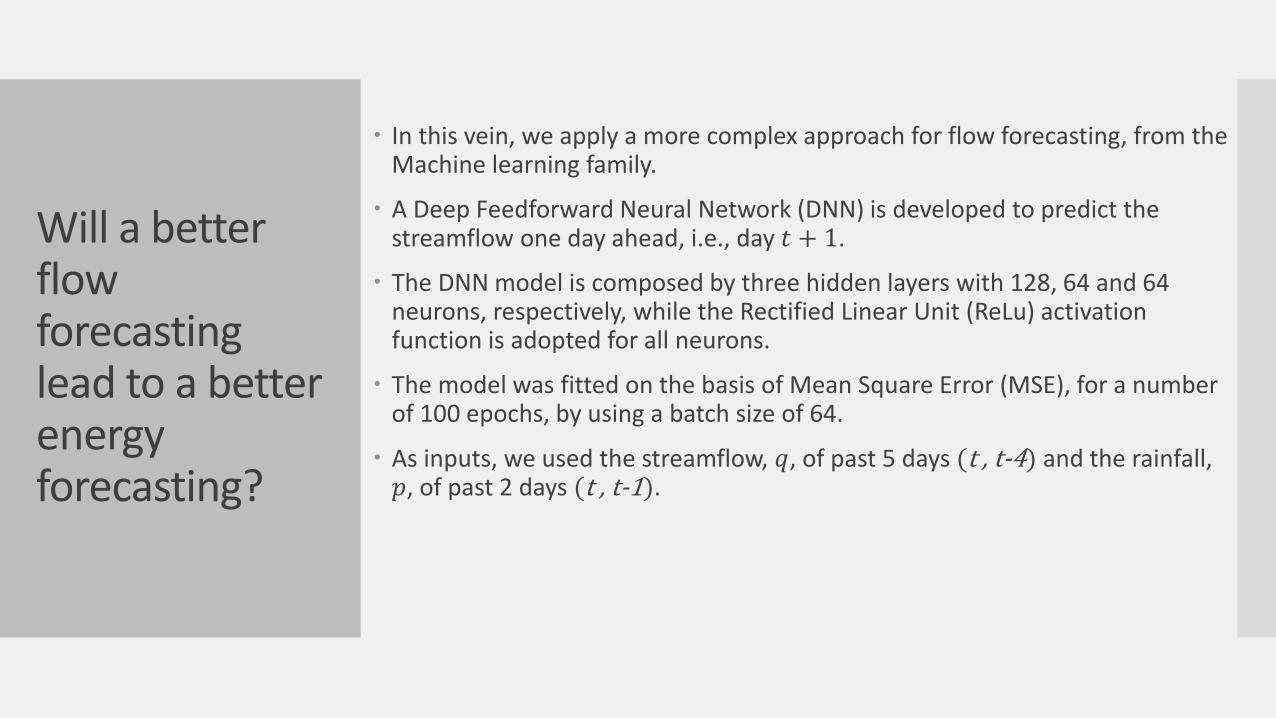
Will a better flow forecasting lead to a better energy forecasting?

In this vein, we apply a more complex approach for flow forecasting, from the Machine learning family.

A Deep Feedforward Neural Network (DNN) is developed to predict the streamflow one day ahead, i.e., day 𝑡 + 1.

The DNN model is composed by three hidden layers with 128, 64 and 64 neurons, respectively, while the Rectified Linear Unit (ReLu) activation function is adopted for all neurons.

The model was fitted on the basis of Mean Square Error (MSE), for a number of 100 epochs, by using a batch size of 64.

As inputs, we used the streamflow, 𝑞, of past 5 days (t , t-4) and the rainfall, 𝑝, of past 2 days (t , t-1).

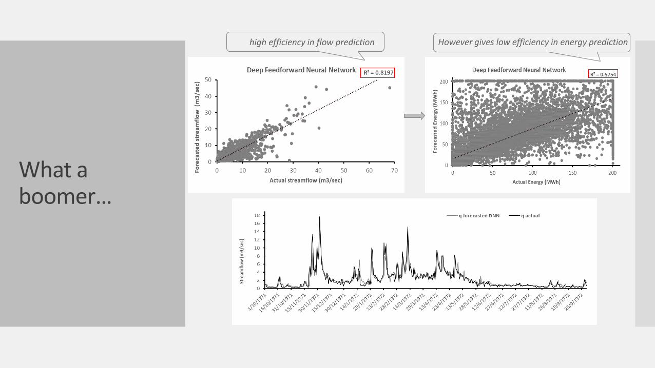
What a boomer…

high efficiency in flow prediction However gives low efficiency in energy prediction

Inserting uncertainty in energy forecast

We use as point estimator the optimal model so far, where its uncertainty is expressed by adding a random error that reproduces the statistical characteristics of model residuals (mean value 𝜇𝑒 , standard deviation 𝜎𝑒, coefficient of skewness 𝛾𝑒).

This error term is generated from a three parameter gamma distribution (i.e., Pearson type III)

𝑓𝑥 𝑥 =𝜆𝜅

Γ 𝜅(𝑥 − 𝑐)𝜅−1𝑒−𝜆 𝑥−𝑐

where κ, λ and c are shape, scale and location parameters, respectively, which are estimated by the method of moments as follows:

𝜆 =𝜅

𝜎𝑒𝜅 =

4

𝛾𝑒2

𝑐 = 𝜇𝑒 − 𝜅/𝜆

• In this case study we generate of 100 energy production ensembles by adding a random term to each point forecasting.

• For each time step (day), we estimate three characteristic quantiles (20, 50, and 80%) from the sample of 100 energy forecasting values.

Energy forecasting in operational context

In a real world energy market, one can take advantage of the median estimation and its bounds to apply three alternative market policies, i.e. risky (80%), mild (50%), and conservative (20%).

For demonstration, we apply the three policies by considering fixed values for the energy produced up to the forecasted value (100 €/MWh), the excess energy production (50 €/MWh) and penalty for deficits (150 €/MWh).

Under this premise, the conservative policy is strongly beneficial while the other two policies lead to economic loss.

Conclusions and perspectives

This research highlights the following issues:

the essential information as input to forecasting;

the dilemma of the energy prediction path, direct or indirect;

the training procedure and the performance measure used in calibration;

the representation of uncertainty and its practical interpretation;

Our analysis indicated the advantages of:

the indirect approach, which embeds a flow prediction tool to the operation model of the hydropower system.

incorporating knowledge about the system operation within calibration.

It is worth mentioning that a high efficiency in flow prediction per se, does not guarantee an equivalently good performance in energy prediction.

Key outcome of this research was the forecasting under uncertainty framework, that can be a guidance for modelling energy market behaviors and support decision-making in the Target model era.