Energy Saving Enhancement of Battery Electric Vehicle over Electrified and Non-Electrified Railway Line by Improving Kinetic Energy Recovery and Reducing Loss on Charging (電化・非電化区間用蓄電池鉄道車両の運動エネルギー回収量 の向上と充電時の損失低減による省エネルギー効果の改善) July 2017 Febry Pandu Wijaya Graduate School of Engineering CHIBA UNIVERSITY
Transcript
Energy Saving Enhancement of Battery Electric Vehicle over
Electrified and Non-Electrified Railway Line by Improving
Kinetic Energy Recovery and Reducing Loss on Charging
(電化・非電化区間用蓄電池鉄道車両の運動エネルギー回収量
の向上と充電時の損失低減による省エネルギー効果の改善)
July 2017
Febry Pandu Wijaya
Graduate School of Engineering
CHIBA UNIVERSITY
(千葉大学審査学位論文)
Energy Saving Enhancement of Battery Electric Vehicle over
Electrified and Non-Electrified Railway Line by Improving
Kinetic Energy Recovery and Reducing Loss on Charging
(電化・非電化区間用蓄電池鉄道車両の運動エネルギー回収量
の向上と充電時の損失低減による省エネルギー効果の改善)
July 2017
Febry Pandu Wijaya
Graduate School of Engineering
CHIBA UNIVERSITY
ii
Name : Febry Pandu Wijaya Registration Number : 14TD2402
Division
Department
: Artificial System Science
: Electrical and Electronics Engineering
Supervisor : Prof. Keichiiro Kondo
Title Energy Saving Enhancement of Battery Electric Vehicle over Electrified and
Non-Electrified Railway Line by Improving Kinetic Energy Recovery and
Reducing Loss on Charging
Keywords
Battery Electric Vehicle, Damping Control, Electrified Railway Line, Energy Saving,
Non-Electrified Railway Line, Regenerative Brake Notch, Wireless Power
Transmission
Abstract
The battery electric vehicle (BEV) for railway has recently attracted much attention
as a method to realize low-cost electrically-driven railway vehicle with high efficiency
and low environmental impact, which is beneficial for through operation over
electrified and non-electrified sections. However, the utilization of onboard battery
storage causes several problems with regards to the increasing vehicle mass and battery
loss. These problems result in increasing the energy consumption of vehicle due to
higher running resistance and higher loss during charging the battery. Therefore, this
thesis proposes three approaches to reduce the energy consumption of BEV at both
running sections. First, the regenerative brake notch method would recover as much
kinetic energy as possible during deceleration, thus reduce the energy consumption of
the vehicle. Second, when running on the electrified section and assuming the battery is
full capacity, the damping control method which keep DC-link voltage of the inverter
high would transmit the regenerative power to a distant load vehicle and thus saving the
substation energy. And third, even when the ground and onboard coils position is
misaligned during wireless battery charging in the non-electrified section, the onboard
charging power control would suppress the increasing charging power, hence reduce the
charging loss and save the consuming energy from the grid. The proposed methods may
contribute to enhance the energy saving of the BEV at both electrified and
non-electrified sections as well as spreading the development of the BEV.
iii
Contents
Abstract ii
Contents iii
1 Introduction 1
1.1 Research Background 1
1.1.1 Current Status of the Energy Source for Railway Vehicle
Traction
1
1.1.2 Application of the Energy Storage Devices in the Railway
Vehicle
2
1.1.3 The Strategies to Solve the Problems of the BEVs 6
1.2 Problems Statement 6
1.3 Research Objectives 9
1.4 Research Contributions 10
1.5 Outline of Thesis 11
2 Advantages and Technical Issues of Regenerative Brake Method at All
over the Speed Range
13
2.1 Introduction 13
2.2 Basic Features of the Regenerative Brake Notch 15
2.3 Driving Assisting Method Based on TICS 22
2.4 Study of Energy Saving Effects by Using Numerical Simulation 28
2.4.1 Energy Saving Effects against Running Distance 28
2.4.2 Energy Saving Effects against Braking Point 29
2.4.3 Energy Saving Effects against Slippery Condition 31
2.5 Conclusions 36
3 Regenerative Brake Control under Light Load Condition Utilizing Over
Voltage Resistor
37
3.1 Introduction 37
3.2 Damping Control Method of Regenerative Brake Control under Light
Load Condition Utilizing Over Voltage Resistor
40
iv
3.2.1 The Regenerative Brake Control under Light Load Condition 40
3.2.2 The Damping Control Method Utilizing OVRe System 42
3.2.3 The Stability Analysis 46
3.3 Verification of the Proposed Method 48
3.3.1 Simulation Setup 48
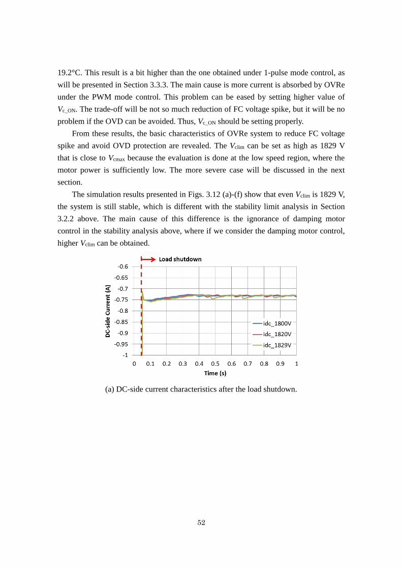
3.3.2 Simulation Results at the Low Speed Region 50
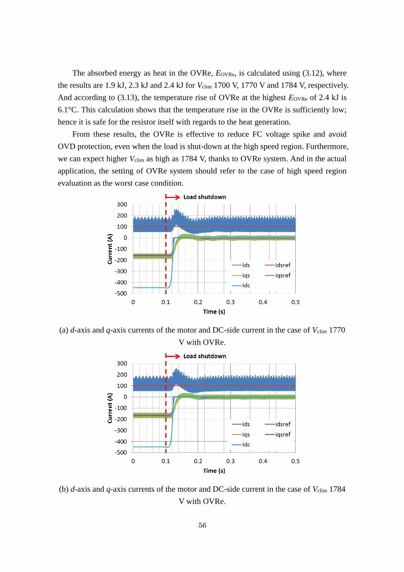
3.3.3 Simulation Results at the High Speed Region 54
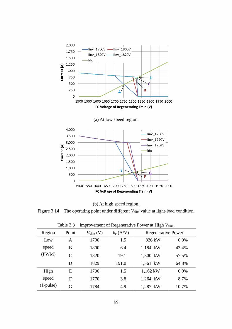
3.3.4 The Regenerative Brake Power Improvement 58
3.4 Conclusions 60
4 A Simple Active Power Control for High Power Wireless Power
Transmission System Considering Coil Misalignment and Its Design
Method
61
4.1 Introduction 61
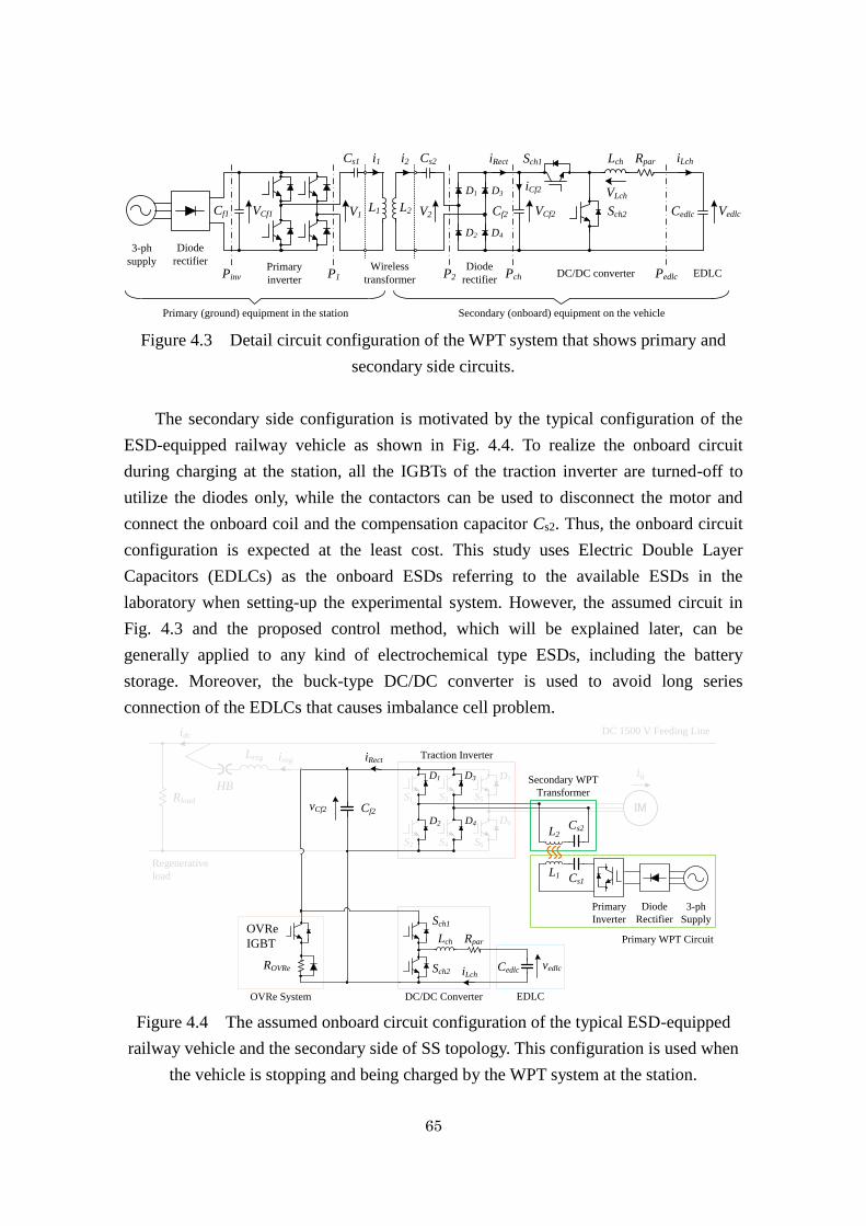
4.2 Wireless Power Transmission System 63
4.2.1 Configuration of the WPT System 63
4.2.2 Equivalent Circuit of the Wireless Transformer 66
4.2.3 Characteristics of the Series-Series Topology 67
4.2.4 Problems of the Conventional Constant Secondary DC-Link
Voltage Control for the Series-Series Topology
68
4.3 Transmission Power Controller and Its Design 70
4.3.1 Control Method of the Transmission Power 70
4.3.2 Method to Design the Control Gains 72
4.4 Verification of the Proposed Control Method 74
4.4.1 Experimental Setup of 100 W System 74
4.4.2 Experimental Results of 100 W System 77
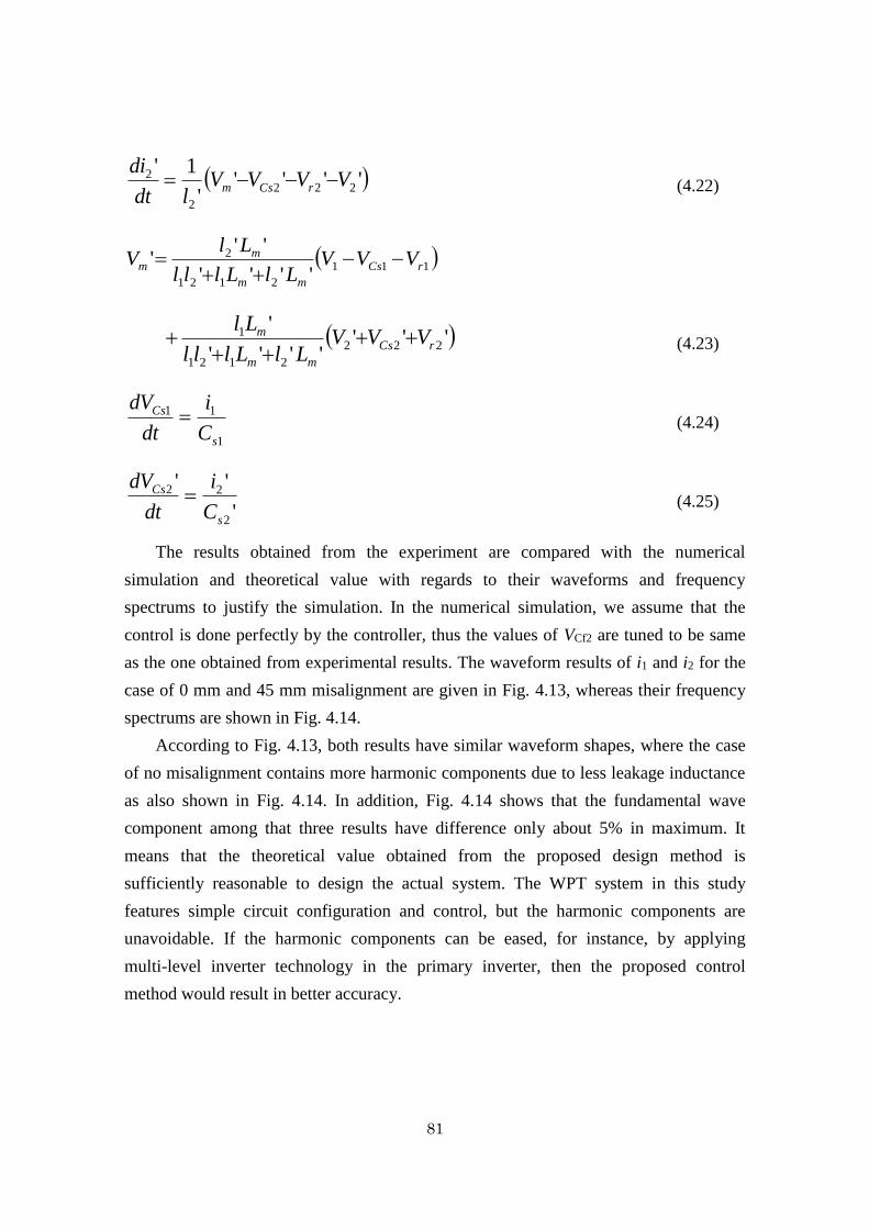
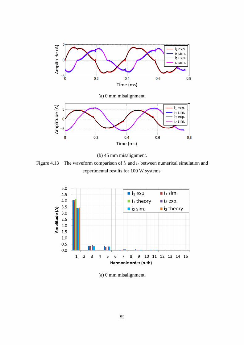
4.4.3 The Comparison between Experimental and Simulation Results 80
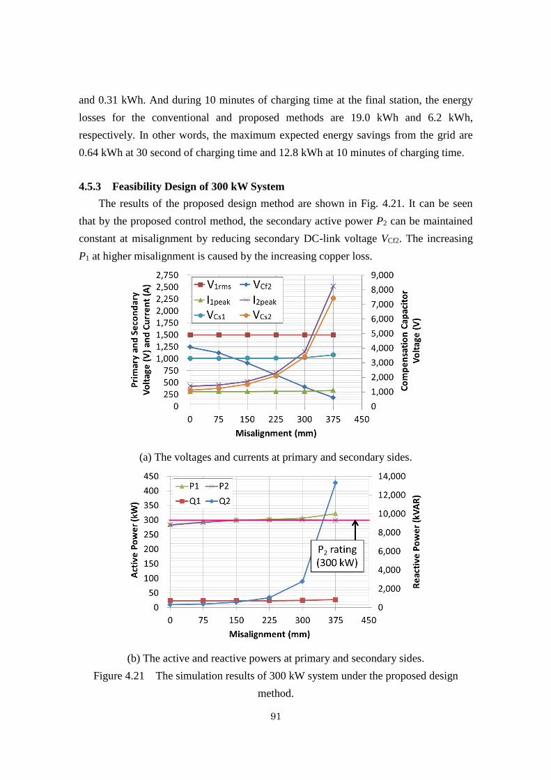
4.5 Theoretical Design of 300 kW WPT System 84
4.5.1 Simulation Setup of 300 kW System 84
4.5.2 Simulation Results of 300 kW System 86
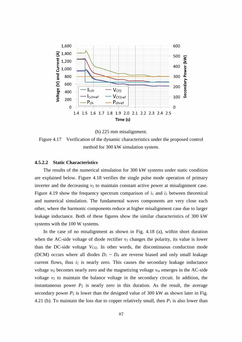
4.5.2.1 Dynamic Characteristics 86
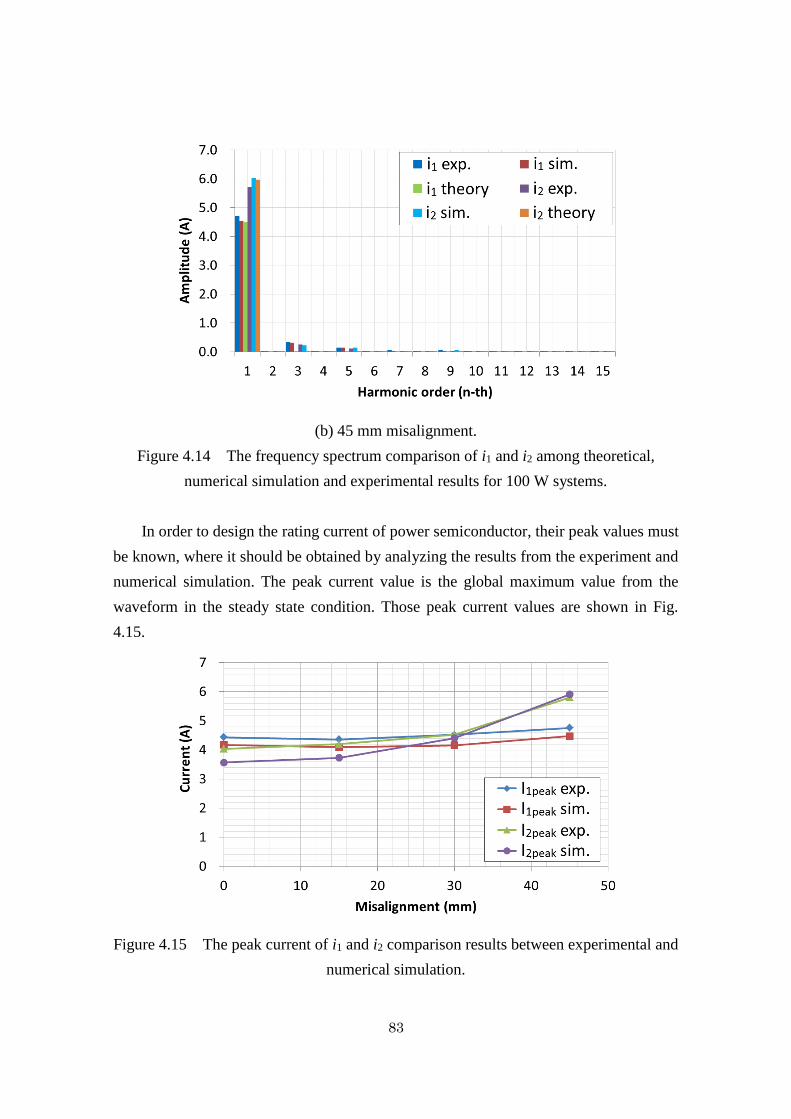
4.5.2.2 Static Characteristics 87
4.5.2.3 Efficiency and Power Loss Characteristics 89
4.5.3 Feasibility Design of 300 kW System 91
4.6 Conclusions 92
v
5 Evaluation of the Proposed Methods to the Target System of EV-E301
Series
94
5.1 Simulation Setup 94
5.2 Simulation Results and Discussion 96
5.2.1 Energy Saving Effects due to the Regenerative Brake Notch 96
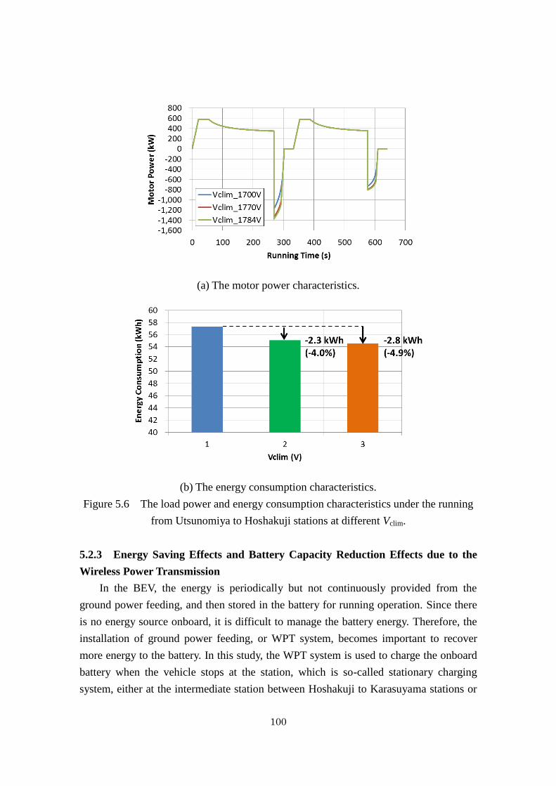
5.2.2 Energy Saving Effects due to Higher Vclim under the Light-load
Regenerative Brake Control
98
5.2.3 Energy Saving Effects and Battery Capacity Reduction Effects
due to the Wireless Power Transmission
100
5.2.3.1 Energy Saving Effects under the Conditions of 100%
of Battery Energy Capacity and 80% of Initial
Battery Energy
103
5.2.3.2 Energy Saving Effects under the Conditions of 100%
of Battery Energy Capacity and Different Initial
Battery Energies
105
5.2.2.3 Energy Saving Effects under the Conditions of
Different Battery Energy Capacities and 80% of
Initial Battery Energy
108
5.2.2.4 The Summaries of Cost Analysis 110
5.3 Conclusions 110
6 Summary and Future Works 112
6.1 Summary 112
6.2 Future Works 114
Acknowledgements 115
Bibliography 117
Publications 123
1
Chapter 1
Introduction
1.1 Research Background
1.1.1 Current Status of the Energy Source for Railway Vehicle Traction
Nowadays, compared to other transportation systems such as airplane, ship, bus and
private car, the energy efficiency of railway vehicles is already at a very high level.
Even so, there are still many possible solutions to improve it. Generally, the main
principles to improve the energy efficiency are increasing the recovery of regenerative
brake energy and reducing the energy loss. The improvement varies to some fields of
study, such as optimization of the speed profile to effectively use the substation energy,
weight reduction of the car-body and components to reduce the running resistance loss,
the utilization of energy storage device to effectively use the regenerative brake energy,
the use of SiC inverter to reduce the power converter loss and so on [1], [2].
According to the electricity supplied for the train operation, the railway network
could be categorized into electrified line, non-electrified line, and mix-line between
electrified and non-electrified. In the electrified railway network, the energy is supplied
to the vehicle continuously through current collectors, either by overhead wire or third
rail mounted at track level. This energy is generated from the power plant, which is then
transmitted and distributed to several numbers of substations. The initial cost to electrify
the railway line as well as the maintenance cost along the line is very high, which
becomes the reason why the electrification is mostly applied at regions with high traffic
density, such as urban and suburban areas. In this network, due to the use of electric
traction system, the regenerating train is able to transmit the regenerative power to the
adjacent powering train; hence it could save the substation energy. By far, this Electric
Motive Unit (EMU) system is the most energy efficient and environmentally friendly
railway transportation system. However, the EMU is not an autonomous vehicle, where
it could only run at the designated railway network.
As the comparison, the non-electrified railway line is beneficial for regions with
low traffic density, such as rural area. In 2012, the share of non-electrified railway
networks all over the world is quite high, which is around 68% of the total lines of 1.7
2
million km, and the growth of electrified lines is only around 1% per year [3]. This fact
causes the autonomous feature is important for the future railway vehicle. In the
non-electrified line, the electrification cost is tackled by equipping the vehicle with
onboard prime mover as the energy source, which is so-called the diesel engine. Thus,
the vehicle itself has an autonomous feature, where it could go anywhere it could as
long as the fuel is sufficient. However, since the tractive force is transmitted to the
wheel through hydraulic transmission, there is no option to recuperate the regenerative
brake energy; hence, less efficient. Other issues of this Diesel Motive Unit (DMU)
system include lower performance, limited power density of diesel engine,
environmental impacts (i.e. the fuel consumption and the emission of CO2, NOx and
SOx), noise, and periodical maintenance of the mechanical equipment. Although there
are drawbacks of the non-electrified railway system, it is impossible to electrify all the
lines because it is economically inefficient to invest in the electrification facilities [4].
Thus, realizing low-cost electrically-driven vehicle that combines the energy efficient
and environmental friendly features of the EMU with the autonomous feature of the
DMU is very challenging for the future railway system.
1.1.2 Application of the Energy Storage Devices in the Railway Vehicle
One of the feasible solutions is to use a hybrid technology, where the energy storage
device (ESD) is installed to assist the diesel engine to supply the load power. Generally,
the purposes of hybrid technology are to save the diesel engine energy, which is
equivalent to save the fuel consumption, and to cut the peak power of the diesel engine,
thus smaller size of diesel engine with lower fuel consumption and lower emission
could be used. There are many interesting studies related to this technology, which
could be found in [5]-[9]. In the practical application, at this moment, the hybrid
technology has been already applied in the commercial railway operation. For example,
type KiHA-E200 is the first diesel series-hybrid train in the world operated by JR East
Railway Company, which has been entering the revenue service from 2007 to serve the
Koumi Line in Yamanashi and Nagano prefectures, Japan [10]. This car uses 300 kW
and 15.2 kWh class lithium-ion batteries as the ESD to assist the diesel engine, which
results in around 20% of energy saving in the plain sections and around 10% of energy
saving in the mountainous sections. Other examples are type Regio Class VT642 diesel
parallel-hybrid that is still being tested by Deutsche Bahn in Germany [11], type HD300
diesel series-hybrid shunting locomotives operated by JR Freight Railway Company
[12] and type Green Goat diesel series-hybrid shunting locomotives operated by several
railway companies in the North America [13]. These hybrid technologies are beneficial
3
to save the energy and become the most feasible solution for the non-electrified railway
line, under the current performance of ESD. In the future, according to the study by the
Institute of Applied Energy of Japan, the energy density of batteries would be doubled
by 2030. This progress may provide 500 kW and 30 kW class batteries that would
enable the diesel engine to maintain idling through the running operation, hence
drastically cut the fuel consumption [4]. However, the best solution to cope with the
problems of DMU system is to remove the diesel engine itself. Therefore, the idea of
ESD-equipped railway vehicle without the diesel engine has recently attracted much
attention [14]-[18]. In the future, by referring to that ESD development, the
ESD-equipped railway vehicle may replace the role of hybrid diesel car in the
non-electrified line.
The ESD-equipped railway vehicle is a promising solution to provide the energy
efficient, environmental friendly and autonomous railway vehicle. Among all of the
ESD technologies (e.g. battery, super-capacitor and flywheel), the battery is commonly
chosen due to its higher energy density thus require less charging station. High energy
density of ESD is an important feature because the space and mass of vehicle are
limited. The vehicle itself is called Battery Electric Vehicle (BEV). In this vehicle, the
energy is periodically but not continuously provided from the ground power feeding,
and then stored in the battery for running operation. Because the energy is not
continuously provided, there would be a problem on how to sustain the onboard energy
in the battery. As the results, the battery capacity would be very high to satisfy the
driving range requirement when running on power from battery only. A new built
battery charging facility at several stations, which may increase the total system cost, is
required for the return trip or extending the driving range of BEV. One of the low-cost
solutions to minimize the number of battery charging station is connecting the BEV to
the existing electrified line, so as to charge the battery while running in the electrified
line. Thus, at this moment, the practical application of BEV is still limited for through
operation over electrified and non-electrified sections. The purpose of mix-electrified
line itself could be a hub to connect high traffic density in the urban/suburban areas with
the low traffic density in the rural area by a cheaper solution than full electrification. Or
it could be used inside the city center in which the overhead wires must be removed to
preserve the historical building, where this line becomes a non-electrified line.
The basic operation of BEV is that, in the electrified section, the battery is charged
to its full capacity by the ground power feeding for the running in the non-electrified
section. The battery is sized to meet the specified driving range of the vehicle in the
non-electrified section. Examples of the commercial BEV are given in Table 1.1. In this
4
research, we assume that the target system is EV-E301 series, which is also called as the
conventional BEV. The EV-E301 series is operated in Tochigi prefecture, where it runs
11.7 km in the electrified section of Tohoku main line under 1500 VDC overhead wire
and runs 20.4 km in the non-electrified section of Karasuyama line using onboard
battery. Figure 1.1 shows the running conditions of EV-E301 series.
Table 1.1 The examples of commercial BEV.
Type of train Electrified line
conditions
Non-electrified line
conditions
Development
purpose
EV-E301
(Japan) [19]
11.7 km
1,500 VDC
20.4 km
95 kWh, 300 kW
Contact charging at
turn-back station
Replacing old
DMU system
Increase
connectivity to
rural line
BEC-819
(Japan) [20]
34.5 km
20 kVAC, 60 Hz
10.8 km
41.5 kW, 300 kW
No charging facility
Increase
connectivity to
rural line
EV-E801
(Japan) [21]
13.0 km
20 kVAC, 50 Hz
26.6 km
180 kWh, 300 kW
Contact charging at
turn-back station
Replacing old
DMU system
Increase
connectivity to
rural line
Citadis-302
(France) [22]
7.78 km
750 VDC
435 m and 485 m
27.7 kWh, 200 kW
No charging facility
Preservation of
historical
building
Catenary
Substation
Power lines
Charging
facility
Distribution line
Overhead
conductor rail
In electrified
sectionsIn non-electrified
sections
Runs as
ordinary EMU
while charging
Runs on
power from
batteries
Quick
charges via
pantograph
At turn-back
station
11.7 km 20.4 km
Figure 1.1 The running conditions of EV-E301 series.
5
As explained above that in order to be operated in the non-electrified sections, a
high capacity battery must be installed onboard. However, the utilization of onboard
battery storage causes several problems with regards to the increasing vehicle mass and
battery loss, compared to the conventional EMU. These problems result in increasing
the energy consumption of the vehicle due to higher running resistance and higher loss
during charging the battery.
To study that effect, a comparison of energy consumption between the assumed
BEV and conventional EMU is shown in Fig. 1.2. The assumed BEV parameters are
given in Table 5.1 in Chapter 5, where the vehicle mass including the passengers is
110.0 ton. In the case of 2-cars conventional EMU, the vehicle mass is lighter and
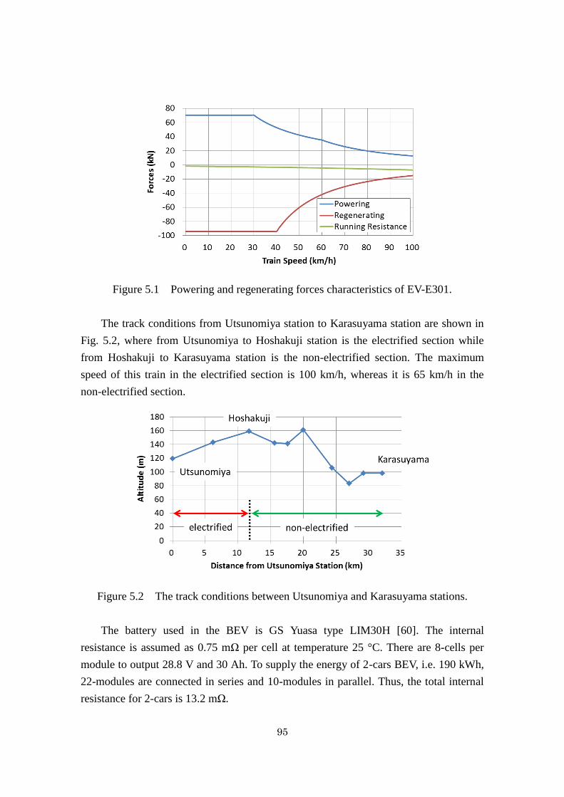
assumed as 96.0 ton. In addition, the tractive forces characteristics and the track
conditions are given in Fig. 5.1 and Fig. 5.2, respectively. In this case, we assumed the
track is non-electrified only when the BEV is operated, whereas it is assumed as
electrified only when the conventional EMU is operated. Moreover, as will be described
in Chapter 5, the internal resistance of battery is assumed as 13.2 mΩ. The characteristic
of energy loss due to battery internal resistance is given in Fig. 1.2 as well.
Figure 1.2 The comparison of energy consumption between conventional EMU and
BEV, and the battery loss in BEV.
Figure 1.2 shows that the energy consumptions of conventional EMU and BEV
under the given conditions are 89.4 kWh and 108.8 kWh, respectively. The difference of
the energy consumption is mainly caused by the difference of mass between
conventional EMU and BEV. The BEV requires higher energy consumption due to
heavier mass, which results in higher running resistance. In this case, the onboard
battery mainly contributes to the increasing BEV mass. In addition, that difference is
6
also caused by the battery loss in the BEV during charging and discharging the battery,
i.e. 3.6 kWh, where this loss is not generated in the conventional EMU due to no
onboard battery storage. These results confirm that the utilization of onboard battery
increases the energy consumption of the BEV compared to the conventional EMU.
1.1.3 The Strategies to Solve the Problems of the BEVs
To cope with these problems, this thesis proposes three approaches to reduce the
energy consumption of BEV at both electrified and non-electrified sections. First, the
regenerative brake notch method would recover as much kinetic energy as possible
during deceleration, thus reduce the energy consumption of the vehicle. This approach
could be applied to both running sections. Second, when running on the electrified
section and assuming the battery is full capacity, the damping control method which
keep DC-link voltage of the inverter high would transmit the regenerative power to a
distant load vehicle and thus saving the substation energy. And third, even when the
ground and onboard coils position is misaligned during wireless battery charging in the
non-electrified section, the onboard charging power control would suppress the
increasing charging power, hence reduce the charging loss and save the consuming
energy from the grid. By applying that approaches, we could expect to enhance the
energy saving of the BEV at both electrified and non-electrified sections as well as
contribute to spread the development of BEV.
The technical issues of the existing BEV as well as the proposal methods would be
explained in more detail in the next section.
1.2 Problems Statement
There are three technical issues in the conventional BEV addressed in this thesis, which
are described in the following:
(1) The first problem is less recovery of kinetic energy from regenerative brake
The regenerative and mechanical brake systems are generally applied in the
railway vehicle, including the BEV, either running in the electrified or
non-electrified sections. The regenerative brake force is weaker at high speed
region due to the limitation of the motor voltage and current. Thus, the mechanical
brake is used mainly at higher speed region to compensate that shortage to obtain
constant deceleration. However, the mechanical brake generates loss as heat at the
wheel and increases the wear of mechanical brake parts.
In order to recover as much kinetic energy as possible to the battery or the
7
adjacent powering train during deceleration, we should avoid the use of mechanical
brake as much as possible. In other words, the regenerative brake only, or so-called
regenerative brake notch, is used to stop the vehicle by applying weaker brake force
in the higher speed region. The regenerative brake notch should be applied earlier
than the constant deceleration brake system in order to arrive at the station under
the same running time. Thus, we could expect to save much kinetic energy and thus
reduce the energy consumption of the vehicle as well as reduce the wear of
mechanical brake parts. However, the nonlinear characteristics of regenerative
brake force results in not constant deceleration at all over the speed range. Hence, it
is difficult for the driver to find the correct starting braking position manually. To
cope with these problems, this study proposes a method to assist the driver finding
the correct starting braking position by means of the preinstalled train information
and control system (a kind of GPS system). The data obtained from this navigation
system is used to generate an imaginary train that run along with the real train to
estimate the real train braking pattern. By means of this method, only the point to
start braking is required and the driver could regulate the brake force in the lower
speed range to stop the vehicle at the station.
(2) The second problem is less utilization of substation energy in the electrified section
When the BEV is running in the DC-electrified section, the battery is charged
either by overhead wire on powering period or by regenerative brake to ensure that
the battery energy is sufficiently high for running in the non-electrified section. To
prevent from overcharging that would destroy the battery cells; the battery must
have limitation on its charging energy or voltage. Thus, if this upper limit is reached
or it cannot absorb more energy, the charging energy to the battery will be stopped
and the BEV operation would be same as a normal EMU in the electrified section.
If this condition occurred during regenerative brake period, the vehicle must supply
the electricity to the adjacent powering vehicle because the diode rectifier is
generally applied in the substation.
Although reaching the upper limit may be not so frequent, but it is difficult to
be completely avoided under the limited battery capacity because the charging
energy to the battery may vary in the actual running depending on the load
conditions, for example braking in the downhill gradient consecutively. There
would be a solution to lowering the upper limit of battery energy, but this is not an
interesting solution because it reduces the usable capacity of the battery. Thus, the
condition that the battery cannot absorb more energy during regenerative braking in
8
the DC-electrified section should be considered in the traction system design of
BEV.
Assuming that condition, the problem arises when the regenerating power
exceeds the load power, for example the powering train suddenly changes its
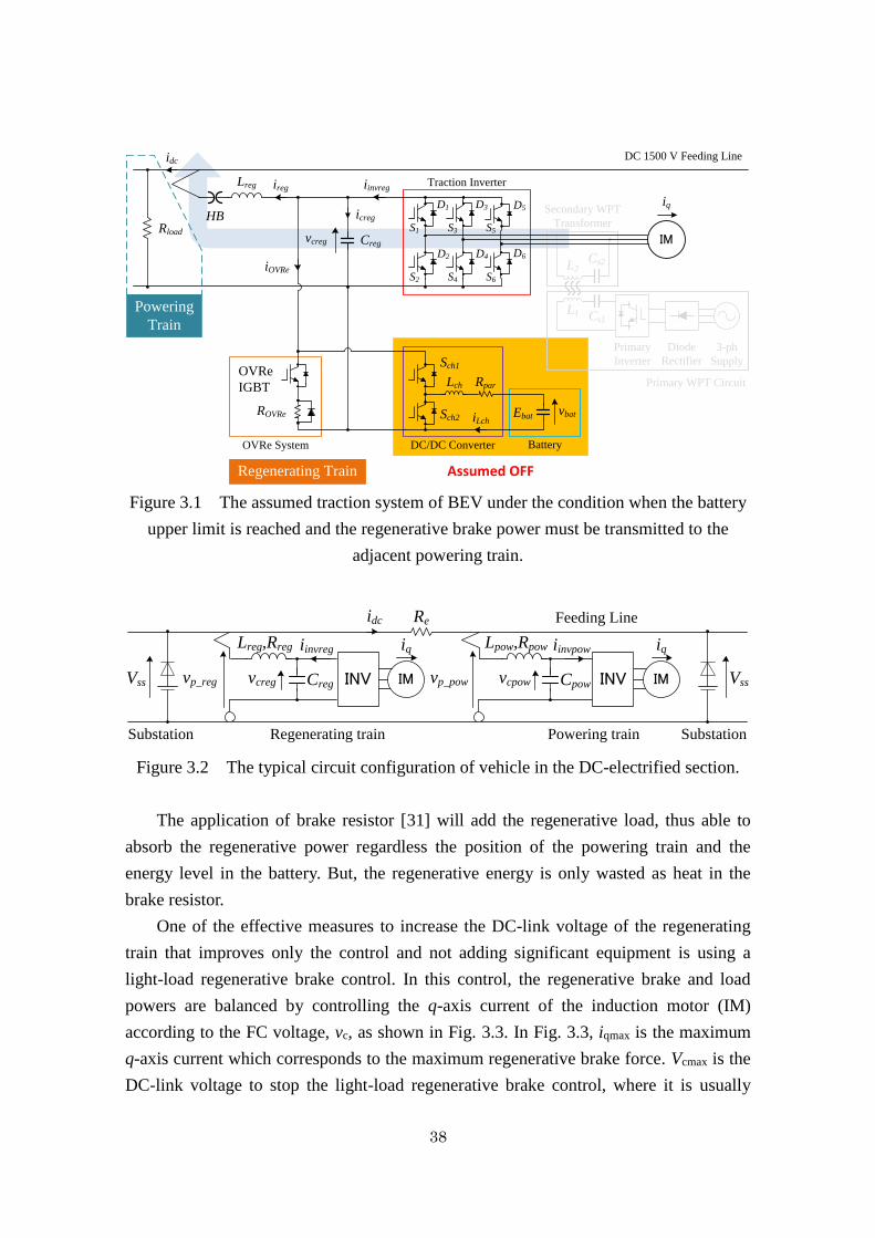
operation from powering to coasting. In this case, the filter capacitor (FC) voltage
of the traction inverter increases. It sometimes reaches to the upper limit and
activate the over voltage protection (OVD), which then utilize the substation energy
to supply the powering train. The light-load regenerative brake control is an
effective measure to solve this problem, where it reduces the regenerative brake
force by controlling q-axis current of the induction motor to balance the
regenerative brake and load powers.
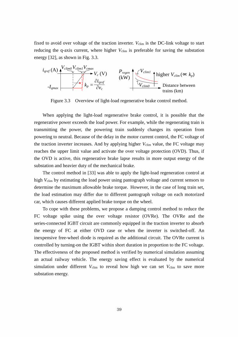
In this control, the design value of the FC voltage to start the regenerative
brake control (or Vclim) is important which determines the amount of regenerative
brake power, where higher Vclim is preferable for saving the substation energy. In
other words, to transmit higher current to the distant powering train, the DC-link
voltage of regenerating train must be kept high to compensate the voltage drop in
the feeding line. However, higher Vclim is equivalent to higher feedback control gain,
where if the regenerating loads changes suddenly, it results in more rapid change of
the motor current. And due to the delay in the motor control, it increases the FC
voltage and may activate the OVD. This regenerative brake lapse results in more
output energy from the substation and heavier duty of the mechanical brake. To
cope with these problems, this study proposes a damping control method to reduce
the FC voltage spike using the over voltage resistor (OVRe), which is commonly
equipped in the traction inverter. The evaluation is done under the load shutdown as
the worst case condition of sudden load change. The excess current that flows to the
FC at the load shutdown, due to delay in the motor current control, is then absorbed
by OVRe. As the results, the spike of FC voltage is reduced, OVD protection is
avoided, and the Vclim could be set to higher value to save more substation energy.
Moreover, the design criteria of Vclim under the worst case conditions could be
clarified.
(3) The third problem is higher power loss in the battery during charging
Generally, low battery capacity and long distance driving range of BEV are
desirable. However, the regenerative brake energy is not sufficient to compensate
the running energy loss; even the regenerative brake notch is used. Thus, as one of
the solutions, the battery charging station in the non-electrified section is required.
9
But, the existing charging station that uses contact wire has problems with high
power, long charging time and the contact wire itself. Therefore, a low power, fast
and frequent charging time is an attractive option. To avoid the maintenance work
and safety problem associated with the contact wire, a wireless power transmission
(WPT) system is proposed.
In the WPT system, one of the technical issues is how to suppress the
increasing charging power when the ground and onboard coils position is
misaligned due to imprecise stopping at the station. The increasing charging power
corresponds to the increasing battery loss and the energy consumption from the grid.
In addition, not only the active power will increase at coil misalignment case, but
also the reactive power and the total capacity of power converters.
To cope with these problems, this study proposes a simple constant secondary
active power control method, which is able to maintain the active power of onboard
converter even at coil misalignment. The control is developed under simple circuit
configuration at both primary and secondary sides, including the simple
Series-Series (SS) WPT topology. Under the constant secondary current feature of
SS topology, where its value is proportional to misalignment distance, suppression
of the increasing secondary active power at misalignment to its rating value is done
by regulating the secondary DC-link voltage according to the active power rating
and secondary current. The control method is designed using fundamental wave
component analysis for simplicity. Afterwards, under that simple control, this study
proposes a method to design the capacity of the power converters considering the
harmonic components. As the results, the design criteria of the rating voltage and
current of the primary and secondary side power converters can be determined.
Moreover, the total converter capacities are reduced, where the current rating of
IGBTs, diodes and compensation capacitors are sufficiently low compared to the
conventional constant secondary DC-link voltage control method. Furthermore, the
suppression of charging power at coil misalignment would reduce the power loss in
the battery as well as the consuming energy from the grid.
1.3 Research Objectives
The objective of this thesis is
“To clarify the methods to save the energy consumption of the Battery Electric
Vehicle by recovering more kinetic energy during regenerative brake and reducing
the battery loss while charging”
10
The sub-objectives of this thesis are:
To develop a method for recovering as much kinetic energy as possible to the
battery or powering train during regenerative brake to reduce the energy
consumption of vehicle
To develop a method for increasing the DC-link voltage of regenerating train to
transmit more regenerative power to distant load vehicle as well as saving the
substation energy
To develop a method to suppress the increasing charging power of WPT system at
coil misalignment and clarify the design method of power converters’ capacity in
order to reduce the battery loss and save the consuming energy from the grid
This thesis uses the Battery Electric Vehicle as a target system for the evaluation.
However, the proposed methods could also be applicable to the other types of vehicles
as long as the assumed conditions could be applied. For example, the regenerative brake
notch method is applicable to any kind of railway vehicles that use electric traction
motor. In addition, the proposed damping control of light-load regeneration control
using OVRe system is also beneficial to save the substation energy in the conventional
EMU network. Furthermore, the proposed constant active power transmission control at
coil misalignment and the design method of power converters’ capacity is generally
applicable to the WPT-based electric vehicle, such as railway vehicles and automobile
applications.
1.4 Research Contributions
The proposed methods in this thesis deal with saving the energy consumption of the
Battery Electric Vehicle (BEV) by improving the recovery of kinetic energy and
reducing the battery loss on charging. The proposed regenerative brake notch and the
damping control utilizing over voltage resistor methods may contribute to improve the
recovery of kinetic energy during deceleration. This kinetic energy will be transformed
into electrical energy, which can be then either use for driving another accelerating train
in the DC-electrified railway network or save to the battery for next vehicle acceleration
period. And the proposed constant active power control method for WPT system at coil
misalignment case may contribute to reduce the battery power loss during charging in
the non-electrified line, hence saving the consuming energy from the grid. These three
methods are related to the optimization of the power flow on the vehicle itself to save
the consuming energy from the grid.
11
By saving the grid energy, we are able to reduce the environmental impacts, i.e. the
fuel consumption and the emission of CO2, NOx and SOx, to generate the grid energy.
And by enhancing the energy efficiency of the BEV through the proposed methods in
this thesis, the development of the BEV can be more spread out all over the world. Thus,
the BEV can be used not only for connecting the existing electrified and non-electrified
railway network with much less cost than full electrification as in the current status, but
also to replace the role of Diesel Motive Unit in the future non-electrified railway
network.
1.5 Outline of Thesis
This thesis is divided into six chapters, where the contents of each chapter are
summarized below:
Chapter 2: This chapter describes the advantages and technical issues of the
regenerative brake method at all over the speed range. The driver assisting method
to find the correct starting braking point based on train information and control
system is presented. The energy saving effects of this proposed method is compared
with the conventional constant deceleration brake method in terms of running
distance, error of starting braking point and rail adhesion coefficient using
numerical simulation. This chapter is related to the publication in J-1.
Chapter 3: This chapter presents a damping control method for the light-load
regenerative brake control utilizing the over voltage resistor (OVRe). The methods
to control the OVRe system using high pass filter and hysteresis control are
described. The comparison results by numerical simulation under the condition of
load shutdown between the case without and with OVRe system are presented. It is
revealed that the OVRe could be effectively utilized to reduce the filter capacitor
(FC) voltage spike and avoid the over voltage protection. From these results, the
maximum allowable FC voltage to start the regenerative brake control (Vclim) is
revealed. Furthermore, the improvements of regenerative brake power at high Vclim
are shown. This chapter is related to the publication in L-1 and C-3.
Chapter 4: This chapter discusses a simple active power control for high power
wireless power transmission (WPT) system considering coil misalignment and its
design method. A simple secondary active power control method that is able to
transmit constant active power to some extent of misalignment is presented,
12
including the method to design the control gains. The experimental setup and
results of 100 W WPT systems are given to verify the proposed control method.
The numerical simulation that considers the harmonic components is developed to
be compared and justified by the experimental results. Afterwards, the simulation
setup and results of 300 kW WPT systems assuming actual railway vehicle
application are presented. The battery loss comparison between conventional and
proposed methods will be analyzed. Furthermore, the feasibility design of 300 kW
WPT system is provided to reveal the design criteria of rating voltage and current
of the power converters. This chapter is related to the publication in C-1, C-2 and
J-2.
Chapter 5: This chapter describes the energy saving effects evaluation of the
proposed methods to the target system of EV-E301 series, for both electrified and
non-electrified sections. The discussion of the reasonable WPT power and
installation places against the energy saving effects is presented.
Chapter 6: This chapter summarizes the thesis and suggests future extensions of the
presented approaches.
13
Chapter 2
Advantages and Technical Issues of Regenerative Brake Method
at All over the Speed Range
2.1 Introduction
In the electric traction-based railway transportation system, there are various
possibilities to reduce the energy consumption of the vehicle, for instance saving the
regeneration energy to the energy storage devices (ESDs), either onboard [23], [24] or
wayside [25], [26] in the electrified section, and the use of pure regenerative brake to
stop the vehicle [27]. The energy consumption of ESD-equipped vehicle can be reduced
by the use of regenerative energy for powering phase. However, this technology
requires additional equipment with high initial cost. The pure regenerative brake has a
merit due to the use of inheritance features of traction motor; hence no additional
equipment is required. The principle to save the energy is to use the regenerative brake
only to stop the train and avoiding the use of mechanical brake as much as possible.
Thus, we could expect to save much kinetic energy and thus reduce the energy
consumption of the vehicle as well as reduce the wear of mechanical brake parts. This
study discusses the advantages and technical issues of the pure regenerative brake
method.
In the brake control of electric traction-based railway vehicle, the constant brake
force that combines regenerative and mechanical brake forces is commonly applied. The
constant brake force reference is generated according to the driver’s command in the
cabin, e.g. from notch 1 to 7, where higher number means stronger brake. Since the
traction motor power is limited by the inverter voltage and current, hence the
regenerative brake force in the high speed range is limited. This characteristic is shown
in Fig. 2.1. In this condition, the mechanical brake force compensates the shortage of
the regenerative brake force to obtain constant deceleration. Thus, much kinetic energy
is dissipated by the stronger mechanical brake in the higher speed range which leads to
more heat generation at the wheel and wear of the mechanical brake parts. We can
expect to save the kinetic energy and to reduce the wear of mechanical brake parts, if
14
the weaker brake force is applied in the higher speed range in accordance with the
regenerative brake torque versus speed characteristics of the traction motors. Since this
technology is related to the traction motor characteristics, thus it can be generally
applied to the electric traction-based railway vehicles, such as the Electric Motive Unit
(EMU) and the Battery Electric Vehicle.
Figure 2.1 The characteristics of traction motor.
One of the measures to achieve weaker brake force in the higher speed range and
stronger brake force in the lower speed range is to inform the driver to apply brake
notch with lower number in the higher speed range and higher number in the lower
speed range based on pre-calculated running reference curves and train position
measured by GPS [28]. This measure is called power limited brake. In this system, the
driver is informed which brake notch to be selected by the train operation assistance
system which acquires the train position and speed information from GPS. This method
has a great benefit where no modification of the vehicle is required. However, the
drawback is that the regenerative brake force is only applied by the step and always less
than the maximum regenerative brake performance. Another drawback is that duty of
the driver becomes heavy to follow the instruction to apply certain brake notch based on
position and speed measured by GPS.
In this study, the authors propose “regenerative brake notch” method which follows
the maximum regenerative brake force according to vehicle speed. The benefit of this
system is always utilizing the maximum regenerative brake force featured by the
traction motor characteristics. In this method, the driver only applies the regenerative
brake notch one time and will not be instructed to change the brake notch until the
vehicle speed reduces to lower speed range. Since the regenerative brake notch does not
Torque
Power
Voltage
Constant
torque region
Constant
power region
Characteristics
region
Train speed
regenerative
mechanical
Required
brake for
constant
deceleration
15
generate constant deceleration all over the speed range, hence it is difficult to find the
starting braking point and inform to the driver. There will be a lot of storing data in the
controller that is calculated offline using motion equation by comparing each
combination of train speed and distance because the initial braking speed varies
according to the track conditions, such as gradient, curve, speed limit and adhesion
coefficient. In other words, the calculation load of the controller is high.
To cope with this problem, the authors propose the utilization of imaginary train in
combination with the preinstalled train information control system (TICS) to obtain the
correct starting braking point and inform to the driver. The calculation is done onboard
through TICS by making an imaginary train that run along with the real train by
considering the track conditions. The purpose of imaginary train is to estimate the
braking pattern of the real train that is calculated beforehand in the powering phase of
the real train. In other words, the powering phase of the imaginary train represents the
braking characteristics of the real train under the condition of regenerative brake notch.
The running profiles of these trains are then compared to obtain the correct starting
braking point. By means of this method, only the point to start braking is required and
the driver can regulate the brake force in the lower speed range to stop the train at the
station if required. The energy saving effect by the regenerative brake notch is compared
with the conventional constant deceleration brake notch in terms of running distance,
error of the starting braking point and rail adhesion coefficient. Through the calculation
study, the energy saving effect and usefulness of the proposed regenerative brake notch
is revealed.
2.2 Basic Features of the Regenerative Brake Notch
In this chapter, the basic characteristics of the regenerative brake notch is studied
and compared with the constant deceleration brake notch. In this study, we use
EMU-type vehicle as the assumed railway vehicle, where the proposed method can be
generally applied to the BEV. The vehicle model used in the simulation for that
comparison is explained in the following. First, the configuration of main component in
the EMU-type vehicle is shown in Fig. 2.2.
16
Figure 2.2 Configuration of the main components in the assumed railway vehicle.
A brief description of the main components in Fig. 2.2 is given in the following.
The vehicle is an EMU-type which is operated in the DC 1500 V electrified line. The
energy is continuously supplied from the main source to the vehicle through a
pantograph. The power in the input side is denoted as Pin (W), whereas vin (V) is the
pantograph voltage that is assumed constant as 1500 V for simplicity and iin (A) is the
DC input side current. Since there is a filter capacitor (FC) inside the inverter and the
auxiliary power supply (APS), a filter reactor (FL) is inserted to avoid high di/dt when
connecting those capacitors with the DC main source in parallel. In addition, the LC
circuit composed by that FL and FC is installed to prevent leakage harmonics current
from the inverter that sometime interfere the signal current on rails when detecting the
trains by wayside signaling system. Moreover, the internal resistance in the FL, Rfl (Ω),
is sufficiently high, where it is assumed as 0.1 Ω, which causes high power loss in the
FL, Pflloss (W).
The traction inverter is used to control the operation of the traction motor (M),
where its power is expressed as Pinv (W). Pinv is positive when the vehicle is
accelerating and it is negative when decelerating. The efficiency of inverter, ηinv, is
assumed constant as 0.98. The traction motor converts the electrical energy to the
mechanical energy to rotate the wheel (W) through gear unit (GU). Pmot (W), Pgu (W)
and Pw (W) respectively represent motor power, gear unit power and wheel power. The
efficiency of these equipment are regarded as constant, where they are 0.90 and 0.98 for
efficiency of traction motor, ηmot, and efficiency of gear unit, ηgu, respectively. In
addition, the APS is used to supply the power of auxiliary loads, Paps (W), e.g. air
conditioner, air compressor, and lighting.
The power flow in the circuit in Fig. 2.2 is calculated using the following equations,
where Paps is assumed constant as 30 kW per car.
MInverter
FL
APS
GU W
Auxiliary
Loads
iin
vin
Pin
Pinv
Paps
Pflloss
Pmot Pgu Pw
DC 1500V
17
apsinvfllossin PPPP (2.1)
flinflloss RiP 2 (2.2)
brakingP
poweringP
P
wgumotinv
gumotinv
w
inv
,
,
(2.3)
ininin ivP (2.4)
The energy consumption in the vehicle, Ein, can be simply calculated by integrating
Pin. This equation is used when calculating the energy saving effect in Section 2.4.
dtPE inin (2.5)
In order to simulate the vehicle running, the Newton’s second law of motion is used,
which is given in (2.6). The numerical simulation itself is done under C/C++ language
environment.
dt
dvmFF t
trt
(2.6)
In (2.6), Ft (N) is the traction and braking forces which are specified by the traction and
regenerative brake curves as shown later in Fig. 2.3, mt (kg) is the total mass of train
and vt (m/s) is the train speed. In addition, Fr (N) is the total train resistance which is
sum of running resistance, Frr (N), gradient resistance, Frg (N), and curve resistance, Frc
(N). Moreover, (2.6) is applicable for all operation modes of the vehicle, i.e. powering,
coasting and braking. In the case of coasting, Ft is 0 N which means the vehicle
decelerates depend on its inertia.
By referring to Fig. 2.3 as an example of traction and braking forces, the value of Ft
for the whole vehicle speed range is calculated using (2.7), which is composed of
constant torque region (0 ≤ vt ≤ 35 km/h), constant power region (35 km/h < vt ≤ 65
km/h) and characteristics region (65 km/h < vt ≤ 120 km/h). In (2.7), wp1 (km/h) and
wp2 (km/h) are the weakening points where the value of Ft is weakened after that point
or vehicle speed due to changing the operating region. In this system, wp1 is 35 km/h,
whereas wp2 is 65 km/h. In addition, a (m/s2) is the vehicle acceleration or deceleration
depending on the operating state. Moreover, vtmax is the maximum allowable speed of
vehicle, which is assumed as 120 km/h. But, for the calculation of the regenerative
18
brake notch system in this study, vtmax is assumed as 95 km/h that refers to the maximum
operating speed in the DC-electrified railway network with short distance between each
station.
max221
211
1
,
,
0,
tt
tt
t
t
t
t
tt
t
vvwpv
wp
v
wpam
wpvwpv
wpam
wpvam
F (2.7)
The running resistance, Frr, is expressed using the well-known Davis formula as in
the following equation.
2
ttrr CvBvAF (2.8)
The variables A (N), B (N.h/km) and C (N.h2/km
2) are given in (2.9) to (2.11), where g
(m/s2) is acceleration of gravity, mmot (ton) is mass of the motorized car, mtra (ton) is
mass of the trailer or non-motorized car and n is the number of car per train set. The
coefficients in A, B and C are the typical values used for EMU in Japan [29].
gmmA tramot 78.065.1
(2.9)
gmmB tramot 028.00247.0
(2.10)
gnC 10078.0028.0 (2.11)
The gradient resistance, Frg, is calculated using the following equation.
gradgmF trg (2.12)
In (2.12), the variable grad stands for the gradient defined in per mile (‰). The value of
grad is positive for slope-up and negative for slope-down.
The curve resistance, Frc, can be obtained from the following calculation [29].
curvgmF trc
800
(2.13)
In (2.13), the variable curv stands for the radius of track curve in meter.
The power on the wheel, Pw (W), is simply calculated by (2.14). This power is then
used to calculate the power flow in the vehicle as described above.
19
ttw vFP (2.14)
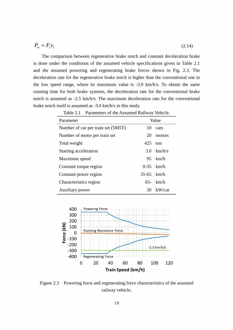
The comparison between regenerative brake notch and constant deceleration brake
is done under the conditions of the assumed vehicle specifications given in Table 2.1
and the assumed powering and regenerating brake forces shown in Fig. 2.3. The
deceleration rate for the regenerative brake notch is higher than the conventional one in
the low speed range, where its maximum value is -3.0 km/h/s. To obtain the same
running time for both brake systems, the deceleration rate for the conventional brake
notch is assumed as -2.5 km/h/s. The maximum deceleration rate for the conventional
brake notch itself is assumed as -3.0 km/h/s in this study.
Table 2.1 Parameters of the Assumed Railway Vehicle.
Parameter Value
Number of car per train set (5M5T) 10 cars
Number of motor per train set 20 motors
Total weight 425 ton
Starting acceleration 3.0 km/h/s
Maximum speed 95 km/h
Constant torque region 0-35 km/h
Constant power region 35-65 km/h
Characteristics region 65- km/h
Auxiliary power 30 kW/car
Figure 2.3 Powering force and regenerating force characteristics of the assumed
railway vehicle.
20
As a comparison example, Fig. 2.4 shows vehicle running profiles with the
regenerative brake notch and the constant deceleration brake notch under the conditions
of equivalent running distance and maximum vehicle speed. In Fig. 2.4 (a), the constant
deceleration brake is applied at 450 m in advance to the station, whereas the
regenerative brake notch is applied at 750 m in advance to the station. In this condition,
the regenerative brake notch requires 300 m longer brake section. Likewise, the
regenerative brake notch requires 10 s longer brake duration as shown in Fig. 2.4 (b). In
addition, the brake force of regenerative brake notch is stronger than the conventional
one in low speed range. Thus, due to longer brake duration and stronger brake force in
low speed range, more kinetic energy can be recovered by regenerative brake notch
method which is shown in Fig. 2.5.
(a) Speed vs. distance.
(b) Speed vs. time.
Figure 2.4 Comparison of the vehicle speed profiles between the regenerative brake
notch and the conventional constant deceleration brake notch.
21
Figure 2.5 The traction motor power of the regenerative brake notch and the constant
deceleration brake notch.
These comparisons reveal that the regenerative brake notch requires more
experience of the driver to stop the train within designated running distance because of
longer brake duration and not constant deceleration rate all over the speed range.
Therefore, some kind of assistance or guidance is required to notify the driver where the
correct starting braking point is. To meet this requirement, the authors propose that the
driver is assisted by the train location information obtained by the preinstalled TICS. By
means of this method, only the point to start braking is required and the driver can
regulate the brake force in the lower speed range to stop the train at the station if
required.
Figure 2.6 shows the system block diagram of the regenerative brake notch system.
In order to operate the regenerative brake notch in the practical situation, a new button
called “regenerative brake notch button” representing the functionality of regenerative
brake notch system can be installed in the driver cabin. Generally, the brake handle is
used for constant deceleration brake by combining regenerative brake and mechanical
brake. By adding this regenerative brake notch button with normally open state, the
driver can apply the regenerative brake notch by pushing that button one time and
followed by operating the brake handle. If the regenerative brake notch cannot be
operated properly to stop the train, for example due to delayed brake point, slippery
condition or the estimated stopping distance can only be covered by the constant
deceleration brake; the driver may apply the constant deceleration brake method.
Afterward, the brake operation will be continued with constant deceleration brake
22
method. Furthermore, in this system, the driver has full responsibility to secure the train
stopping position, either by applying regenerative brake notch or constant deceleration
brake method.
Displays
“regenerative
brake point”
TICS MonitorBrake
handle
Driver Cabin
Calculates
imaginary train
TICS Controller
Generates
brake force
command
TM Controller
Traction
Motor
Slip flag
Regenerative
brake notch
command
Constant
deceleration
brake command
Manual command
by the driver to
apply regenerative
brake notchThe driver operates
regenerative brake
notch one time at
the brake point
Regenerative brake
notch button
Figure 2.6 The system block diagram that shows the tasks of TICS controller, TM
(traction motor) controller and the driver to operate the regenerative brake notch.
2.3 Driver Assisting Method Based on TICS
In the power limited brake method [28], a driving assistance screen is attached in
the cabin to notify the driver which brake notch is to be selected actively. The notch
selection is determined by actively referring to the pre-calculated (off line calculation)
vehicle running profile based on the vehicle position obtained from GPS and the vehicle
speed measured optically from the onboard speed meter. This method features no need
to install any special control function on the vehicle. All of the driver assistance
equipment, such as onboard screen, onboard CCD camera and onboard computer
system to follow the train running profile, can be attached on the existing vehicles. One
of the benefits of this system is suitable for retrofitting the existing vehicles at low cost.
On the other hand, our proposed system is another solution to recover more kinetic
energy without major change of the vehicles or the ground facilities, such as Automatic
Train Operation (ATO) system. The proposed system aims at recently build inverter-fed
AC traction motor system with TICS. As far as these systems are equipped, the retrofit
is possible. In this system, the authors propose the utilization of TICS to calculate the
correct starting braking point to be informed to the driver. The calculation is done
onboard through TICS by making an imaginary train that run along with the real train,
which will be explained later on.
23
The braking distance of the train when applying regenerative brake notch system
can be calculated onboard using motion equation. However, since the regenerating
brake and running resistance forces have nonlinear relationship with the train speed as
shown in Fig. 2.3, there will be a lot of storing data in the controller that is calculated
offline by comparing each combination of train speed and distance because the initial
braking speed varies according to the track conditions, such as gradient, curve, speed
limit and adhesion coefficient. In other words, the calculation load of the controller is
high. In order to reduce the calculation load in the controller, this study uses imaginary
train that takes into account the track conditions which can be obtained from TICS.
The explanations of the imaginary train are given in the flowchart of Fig. 2.7 with
the following description. The purpose of imaginary train is to estimate the braking
pattern of the real train that is calculated beforehand in the powering phase of the real
train. In other words, the powering phase of the imaginary train represents the braking
characteristics of the real train under the condition of regenerative brake notch as shown
in Fig. 2.8 (a). In the former half part of running distance, the imaginary train is
generated by TICS under the same sampling time with the real train using the following
discrete equation. Equation (2.15) is the discrete form of the continuous form of motion
equation in (2.6).
dttsm
tFtFtvdttv
t
rngregenerati
0
002
0
2
0 2 (2.15)
where dt is the sampling time, t0 is the initial time, v(t0) is the initial speed, v(t0 + dt) is
the speed after dt, s(t0 + dt) is the running distance at each dt, Fregenerating(t0) is the
regenerating force of the traction motor, and Fr(t0) is the total train resistance force
including running, gradient and curve resistances. Equation (2.15) models the change of
kinetic energy within short period of dt, such that Fregenerating and Fr are regarded as
constant values because the train speed does not change so much. The running
resistance force Fr uses minus sign because it represents the braking characteristics of
the real train. In addition, this system is assumed to be used for commuter train where
much regenerative loads are expected. Hence, all the regenerative brake power is
assumed to be absorbed by another powering train and Fregenerating in (2.15) uses the
motor characteristics only. Furthermore, when the train is running at the early morning,
at late night or at light load condition, the driver may judge to apply the constant
deceleration brake to stop the train if the regenerative brake notch force is not enough.
24
TICS generates
imaginary train
using Eq. (1)
Start
The real train
starts running from
station A
TICS records the
speed and position
of real train during
running
TICS uses the
stored track
conditions data
from station A
to station B
TM
Controller
output Slip
Flag?
The driver applies
regenerative brake
notch to stop the
real train
The driver may
judge to apply
constant
deceleration brake
The real train
stops at station B
TICS generates
imaginary train
using the assumed
5% of miu on wet
rail condition
TICS generates
imaginary train
using 8.5% of miu
on dry rail
condition
No
Yes
Imaginary
train speed > track
speed limit?
Real train
reaches half of
running
distance?
Yes
Smax is obtained and
reflects the imaginary
train profile as the
braking profile of real
train
Yes
No No
Is braking
point
Z found?
Compare the running
profile of real and
imaginary trains to
estimate braking
point Z
Inform braking
point Z to the
driver cabin
No
Yes
Is regenerative
brake notch force enough
to stop the real train?
End
Yes
No
Imaginary train calculation by TICS
Figure 2.7 Flowchart of the imaginary train calculation by TICS along with the
operation of the real train.
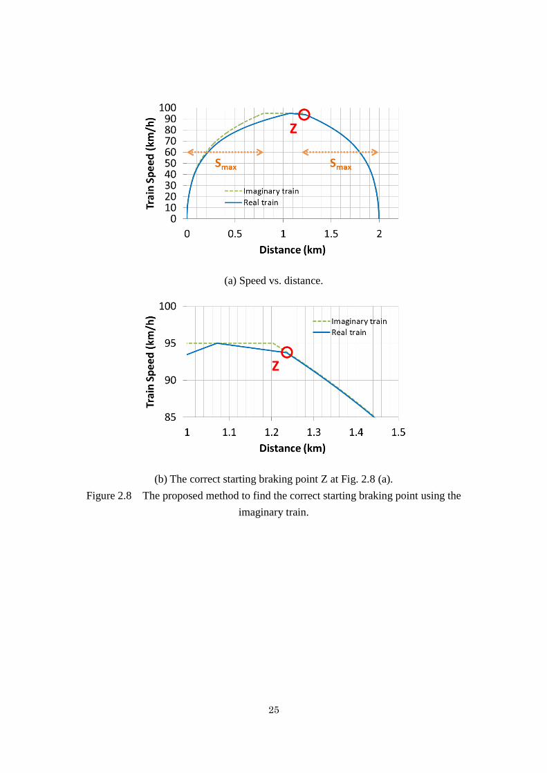
25
(a) Speed vs. distance.
(b) The correct starting braking point Z at Fig. 2.8 (a).
Figure 2.8 The proposed method to find the correct starting braking point using the
imaginary train.
26
(a) Different track gradients.
(b) Different track speed limits.
Figure 2.9 The proposed method to find the correct starting braking point under
different track gradients and speed limits using the imaginary train.
In this case, the track conditions of the real train do not affect the running profile of
the imaginary train because it only uses the same sampling time. The imaginary train
will stop its operation when the speed reaches the maximum allowable speed in the
track, e.g. 95 km/h in this study. At this point, the estimated braking pattern of the real
train is completely generated. The maximum speed of the track is considered, because
the initial braking speed will not exceed this value. Thus, the maximum braking
distance Smax is obtained as well. In the latter part of running distance, when the
remaining running distance of the real train is equal to Smax, the stored pattern of the
imaginary train is reflected to output the imaginary line representing the braking pattern
27
of the real train. The running profiles of these trains are then compared to obtain the
correct starting braking point Z in Fig. 2.8 (b). Please note that Smax is not always same
with the starting braking point Z, because Smax represents the maximum braking
distance when the initial braking speed is the maximum speed, where the initial braking
speed is not always same with the maximum speed.
In addition to the results shown in Fig. 2.8 which is applied to the flat track and
same maximum speed, the imaginary train can also be applied to different track
gradients and different track speed limits as depicted in Figs. 2.9 (a)-(b). From these
results, it can be seen that the imaginary train estimates the condition in the braking part
of the real train, without being affected by the condition in the powering part of the real
train. In other words, as long as the information in the latter half part of the running
distance is obtained beforehand, the imaginary train will be able to estimate the correct
starting braking point during powering phase of the real train. Therefore, from the
results in Figs. 2.8 and 2.9, the imaginary train is sufficiently effective to find the
starting braking point and applying regenerative brake notch under several different
conditions.
The vehicle speed and position information are obtained from navigation function
of TICS. The accuracy of this information is within several meters and few km/h. These
are equivalent with or more accurate than the position and the speed information
obtained from GPS. The accuracy of the position does not affect the performance of the
train speed control because only the starting braking point is required in the proposed
regenerative brake notch method. In this system, the driver is notified by the TICS
several seconds in advance to the correct starting braking point. The major factor of the
error to start the regenerative brake notch may be delay of the driver’s manipulation.
For example, assuming the train speed is 90 km/h, one second delay of the driver’s
manipulation causes 25 m error of the starting braking point. This error can be
compensated by the driver during the train deceleration by selecting the conventional
constant deceleration brake handle. Thus, the accuracy of the train stopping position at
the station is secured by the driver’s brake handle manipulation.
The same principle can be expected in other cases, such as in the steep grade
section where the load condition is larger that requires mechanical brake compensation
by the driver. Another case is when the powering train is less or far from the braking
train. Since the regenerative brake force is limited, the mechanical brake will assist the
regenerative brake notch to stop the train. In the case of the lower adhesive coefficient,
such as rainy or snowy weather, wheel skid is expected especially in the case of
applying stronger brake in the low speed range. Under this condition, the driver may
28
apply the constant deceleration brake notch instead of the regenerative brake notch to
secure the train stopping position. However, this study reveals that under such condition,
even the regenerative brake notch can be applied solely to stop the train at the slippery
rail conditions, which will be described in chapter 2.4.
2.4 Study of Energy Saving Effects by Using Numerical Simulation
In this chapter, the energy saving effects of the proposed regenerative brake notch is
studied by using numerical simulation. To compare properly with the conventional
constant deceleration brake, the maximum speed for both running profiles is assumed
same as 95 km/h. In addition, the running time of constant deceleration brake is
adjusted by changing its deceleration so that coincide with the running time of the
regenerative brake notch. This is because the maximum speed and the running time are
important factors of the energy consumption [30].
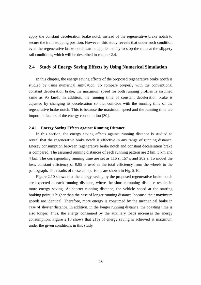
2.4.1 Energy Saving Effects against Running Distance
In this section, the energy saving effects against running distance is studied to
reveal that the regenerative brake notch is effective in any range of running distance.
Energy consumption between regenerative brake notch and constant deceleration brake
is compared. The assumed running distances of each running pattern are 2 km, 3 km and
4 km. The corresponding running time are set as 116 s, 157 s and 202 s. To model the
loss, constant efficiency of 0.85 is used as the total efficiency from the wheels to the
pantograph. The results of these comparisons are shown in Fig. 2.10.
Figure 2.10 shows that the energy saving by the proposed regenerative brake notch
are expected at each running distance, where the shorter running distance results in
more energy saving. At shorter running distance, the vehicle speed at the starting
braking point is higher than the case of longer running distance, because their maximum
speeds are identical. Therefore, more energy is consumed by the mechanical brake in
case of shorter distance. In addition, in the longer running distance, the coasting time is
also longer. Thus, the energy consumed by the auxiliary loads increases the energy
consumption. Figure 2.10 shows that 21% of energy saving is achieved at maximum
under the given conditions in this study.
29
Figure 2.10 Comparison of the energy consumption between the regenerative brake
notch and the constant deceleration brake under the conditions of different running
distance.
2.4.2 Energy Saving Effects against Braking Point
In the ATO system, brake is applied automatically at the correct position. However,
in this regenerative brake notch system, the train driver has to apply the brake notch
manually. The TICS can only inform the driver where the correct starting braking point
is. Therefore, there could be variation of starting braking point. In this section, the
energy saving effects against variation of braking point is studied to reveal that the
proposed TICS-based information system is sufficiently accurate to save the energy. If
the train speed is assumed as 90 km/h when the brake is applied, one second delay of
the driver’s manipulation causes 25 m braking point variation from its correct position.
If the brake is applied 25 m in advance to the correct position, it is able to avoid using
the mechanical brake because the driver reduces the brake force to stop the train at the
station. Therefore, only the case of 25 m closer to the station or the brake is delayed for
1 second should be discussed.
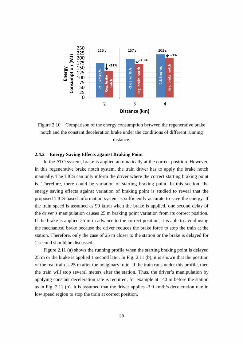
Figure 2.11 (a) shows the running profile when the starting braking point is delayed
25 m or the brake is applied 1 second later. In Fig. 2.11 (b), it is shown that the position
of the real train is 25 m after the imaginary train. If the train runs under this profile, then
the train will stop several meters after the station. Thus, the driver’s manipulation by
applying constant deceleration rate is required, for example at 140 m before the station
as in Fig. 2.11 (b). It is assumed that the driver applies -3.0 km/h/s deceleration rate in
low speed region to stop the train at correct position.
30
(a) Speed vs. distance.
(b) The real train with delayed regenerative brake notch.
Figure 2.11 Comparison of the vehicle speed profiles between regenerative brake
notch and constant deceleration brake in the case of 25 m delay of the braking point
under the same running time.
Figure 2.12 shows the energy consumption in the cases of Figs. 2.4 and 2.10. In Fig.
2.12, the regenerative brake notch with 1 second delay (number 3 from left) has 3% less
energy saving effect that the regenerative brake notch with proper braking timing
(number 2 from left). Even so, 18% of energy saving can be expected compared to the
constant deceleration brake (number 1 from left), which is ineligible energy saving
effect.
The running time with 1 second delayed braking case (115 s) is reduced 1 second
compared to the correct one (116 s) because stronger brake force is applied in low speed
31
region to stop the train. In the right side of Fig. 2.12, the constant deceleration brake of
-2.7 km/h and the 1 second delayed brake are compared to eliminate the effect of
running time. Regenerative brake notch achieves 20% reduction of the consumption
energy even the brake application is delayed for 1 second. Therefore, the proposed
TICS-based information system is sufficiently accurate to save energy using the
regenerative brake notch method.
Figure 2.12 Comparison of energy saving effects between the case of correct starting
braking point and the case of 25 m delayed from starting braking point.
2.4.3 Energy Saving Effects against Slippery Condition
In the slippery condition, stopping the train at the station has more priority than
saving the energy. The driver may apply the constant deceleration brake notch instead of
the regenerative brake notch to secure the train stopping position. However, to gain
more energy saving even at slippery rail condition, the use of regenerative brake notch
should be considered. In this section, the effect of applying the regenerative brake notch
for several slippery rail conditions is discussed.
The information that the train is running on slippery rail can be obtained from the
traction motor controller in the inverter, for example through slip flag signal obtained by
checking the acceleration rate of the wheel or the average motor current, which can be
obtained within few seconds once the train starts running. However, it is difficult to
obtain the information of how much the adhesion ratio in real time is. Therefore, this
study assumes to use 5% of adhesion coefficient when the slip flag is received by TICS
from the traction motor controller regardless the actual adhesion coefficient, which is
sufficiently low compared to 8.5% of adhesion coefficient as the design value of the
32
maximum brake force in this study. In addition, this study assumes uniform adhesion
coefficient along the rail between two stations. The energy saving effect of these
assumptions to different actual adhesion coefficient will be discussed.
The adhesion coefficient (𝜇) is defined as the ratio between traction force per
powered wheel to the axle load, which is given as follows:
g
a
gm
am
t
t
(2.16)
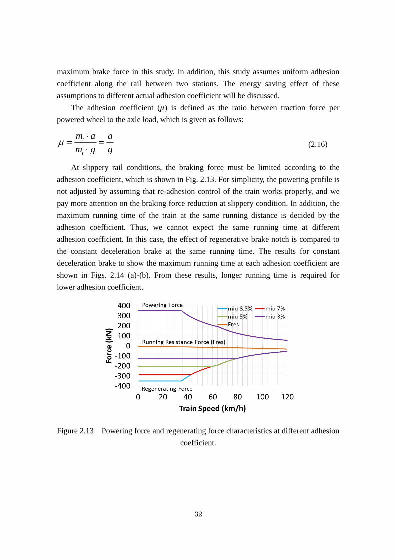
At slippery rail conditions, the braking force must be limited according to the
adhesion coefficient, which is shown in Fig. 2.13. For simplicity, the powering profile is
not adjusted by assuming that re-adhesion control of the train works properly, and we
pay more attention on the braking force reduction at slippery condition. In addition, the
maximum running time of the train at the same running distance is decided by the
adhesion coefficient. Thus, we cannot expect the same running time at different
adhesion coefficient. In this case, the effect of regenerative brake notch is compared to
the constant deceleration brake at the same running time. The results for constant
deceleration brake to show the maximum running time at each adhesion coefficient are
shown in Figs. 2.14 (a)-(b). From these results, longer running time is required for
lower adhesion coefficient.
Figure 2.13 Powering force and regenerating force characteristics at different adhesion
coefficient.
33
(a) Speed vs. distance.
(b) Speed vs. time.
Figure 2.14 Comparison of the vehicle speed profile for constant deceleration brake at
different adhesion coefficient.
34
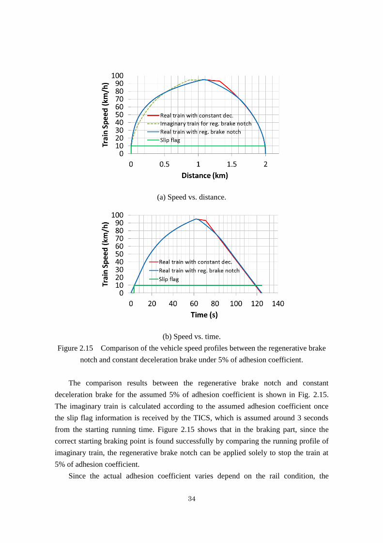
(a) Speed vs. distance.
(b) Speed vs. time.
Figure 2.15 Comparison of the vehicle speed profiles between the regenerative brake
notch and constant deceleration brake under 5% of adhesion coefficient.
The comparison results between the regenerative brake notch and constant
deceleration brake for the assumed 5% of adhesion coefficient is shown in Fig. 2.15.
The imaginary train is calculated according to the assumed adhesion coefficient once
the slip flag information is received by the TICS, which is assumed around 3 seconds
from the starting running time. Figure 2.15 shows that in the braking part, since the
correct starting braking point is found successfully by comparing the running profile of
imaginary train, the regenerative brake notch can be applied solely to stop the train at
5% of adhesion coefficient.
Since the actual adhesion coefficient varies depend on the rail condition, the
35
assumed 5% of adhesion coefficient may have error in estimating the correct starting
braking point and the energy saving effect may deteriorate. The comparison of energy
saving effect between the assumed adhesion coefficient and the actual one, i.e. 7% and
3%, are given in Fig. 2.16. In this case, the slip flag is assumed known when the train
starts running for fair comparison. As seen from Fig. 2.16, by applying weaker brake
force in the low adhesion coefficient, the energy consumption becomes lower, but the
running time is longer.
In case if the actual adhesion coefficient is higher than the assumed one, the starting
braking point is given earlier than expected. In this case, the train can still run and stop
at station using regenerative brake notch only, but the running time is slightly longer, e.g.
8 s in the case between 7% and 5% in Fig. 2.16. For lower actual adhesion coefficient
than the assumed one, the regenerating force becomes higher than allowed. The
re-adhesion control of the train may adjust the regenerating force automatically. In this
case, it is difficult to apply the regenerative brake notch method, where the mechanical
brake is required to stop the train. In addition, the regenerative brake notch method
requires higher vehicle speed to start the braking, because the deceleration rate is lower
than the case of constant deceleration brake. Thus, for lower adhesion coefficient, i.e.
lower than 5% in Fig. 2.13, it is difficult to apply the regenerative brake notch only to
stop the train with the same running time at constant deceleration brake. Under this
condition, the driver may judge which brake method is better to stop the train properly,
either using the regenerative brake notch or the constant deceleration brake. The energy
saving effect in the case of 3% of adhesion coefficient in Fig. 2.16 means that the
regenerative brake notch cannot be applied under this condition.
The energy saving effect for both cases has significant difference with the case of
the assumed adhesion coefficient. Even so, the energy consumption for all cases is
almost equal. For example, higher starting braking speed of 5% adhesion case results in
longer braking time compared to 7% adhesion case, which generally results in lower
energy consumption. However, because the regenerating force of 5% adhesion case is
lower than that of 7% adhesion case, the energy consumption becomes almost equal.
The same principle can be applied for 3% of adhesion coefficient. Thus, since the
energy consumption for all adhesion coefficient cases is almost equal, the assumed 5%
of adhesion coefficient is sufficient to be used at any slippery condition. Therefore, the
proposed regenerative brake notch is also effective to reduce the energy consumption at
the slippery rail condition.
36
Figure 2.16 The comparison of energy saving effect among different adhesion
coefficients.
2.5 Conclusions
To reduce the energy losses by mechanical brake in the high speed region, the
regenerative brake notch system that generates brake torque command equal to the
torque-speed characteristics of the traction motors is proposed in this study. The energy
saving effect is studied by using the numerical simulation. This system achieves 21%
reduction of the energy consumption at maximum under the given conditions.
The authors also propose a train information control system (TICS) based
information system to notify the driver where the correct starting braking point is,
because it is difficult to find the starting braking point manually by the driver. The
imaginary train is used to find the starting braking point by estimating the braking
pattern of real train during the powering phase. The merit of the proposed system is easy
to get the value of speed and position of the train without the need to store a lot of data
in terms of the initial braking speed and distance beforehand.
The effect of braking point variation is studied because this brake is applied not
automatically but manually by the train driver. Even in the late braking case, 18%
reduction of energy consumption is achieved by this system. In addition, the energy
saving effect is also studied for different slippery rail condition. Even though the energy
saving effect is different, but the energy consumption among different adhesion
coefficient is almost equal. At the assumed adhesion coefficient, 13% reduction of
energy consumption is obtained.
Therefore, these results show that the regenerative brake notch method and
TICS-based information system is effective to save the energy of the train operation.
37
Chapter 3
Regenerative Brake Control under Light Load Condition Utilizing
Over Voltage Resistor
3.1 Introduction
When the BEV is running in the DC-electrified section, the battery is charged either
by overhead wire on powering period or by regenerative brake to ensure that the battery
energy is sufficiently high for running in the non-electrified section. To prevent from
overcharging that would destroy the battery cells; the battery must have limitation on its
charging energy or voltage. Thus, if this upper limit is reached or it cannot absorb more
energy on either powering or braking periods, the charging energy to the battery will be
stopped by turning-off the DC/DC converter and the BEV operation would be same as a
normal EMU in the electrified section. If this condition occurred during regenerative
brake period, the vehicle must supply the electricity to the adjacent powering vehicle
because the diode rectifier is generally applied in the substation [24], as shown in Fig.
3.1. Although reaching the upper limit may be not so frequent, but it is difficult to be
completely avoided under the limited battery capacity because the charging energy to
the battery may vary in the actual running depend on the load conditions, for example
braking in the downhill gradient consecutively. There would be a solution to lowering
the upper limit of battery energy, but this is not an interesting solution because it
reduces the usable capacity of the battery. Thus, the condition that the battery cannot
absorb more energy during regenerative braking in the DC-electrified section should be
considered in the traction system design of the BEV.
Assuming that condition and referring to the typical circuit configuration of the
vehicle in the DC-electrified section as shown in Fig. 3.2, to transmit higher
regenerative power to the distant powering train, which then saves the substation energy
to supply the powering train, the DC-link voltage of the regenerating train must be
controlled at higher value to compensate the voltage drop in the feeding line.
38
Figure 3.1 The assumed traction system of BEV under the condition when the battery
upper limit is reached and the regenerative brake power must be transmitted to the
adjacent powering train.
Figure 3.2 The typical circuit configuration of vehicle in the DC-electrified section.
The application of brake resistor [31] will add the regenerative load, thus able to
absorb the regenerative power regardless the position of the powering train and the
energy level in the battery. But, the regenerative energy is only wasted as heat in the
brake resistor. One of the effective measures to increase the DC-link voltage of the regenerating
train that improves only the control and not adding significant equipment is using a
light-load regenerative brake control. In this control, the regenerative brake and load
powers are balanced by controlling the q-axis current of the induction motor (IM)
according to the FC voltage, vc, as shown in Fig. 3.3. In Fig. 3.3, iqmax is the maximum
q-axis current which corresponds to the maximum regenerative brake force. Vcmax is the
DC-link voltage to stop the light-load regenerative brake control, where it is usually
IM
Secondary WPT
Transformer
Traction Inverter
DC/DC Converter
vcreg
iinvreg
Cs2
Sch1
Sch2 iLch
Lch
vbat
L2
D3
D4
D1
D2
Creg
Rpar
Ebat
Battery
S1
D5
D6
S3 S5
S2 S4 S6
icreg
ROVRe
OVRe
IGBT
OVRe System
iOVRe
Primary WPT Circuit
L1 Cs1
Diode
Rectifier
3-ph
Supply
Primary
Inverter
iregLreg
iq
DC 1500 V Feeding Line
Rload
Regenerative
load
idc
HB
Assumed OFFRegenerating Train
Powering
Train
idc Re Feeding Line
Vss
Substation
Vss
SubstationRegenerating train
IMvcreg INVCreg
Lreg,Rreg iqiinvreg
vp_reg
Powering train
IMINVCpow
Lpow,Rpow iqiinvpow
vp_pow vcpow
39
fixed to avoid over voltage of the traction inverter. Vclim is the DC-link voltage to start
reducing the q-axis current, where higher Vclim is preferable for saving the substation
energy [32], as shown in Fig. 3.3.
Pregen
(kW)
Distance between
trains (km)
higher Vclim (∝ kp)
Vclim0
Vclim1iqref (A)
Vc (V)
-Iqmax
VcmaxVclim0 Vclim1
kp = ∂iqref
∂vc
Figure 3.3 Overview of light-load regenerative brake control method.
When applying the light-load regenerative brake control, it is possible that the
regenerative power exceeds the load power. For example, while the regenerating train is
transmitting the power, the powering train suddenly changes its operation from
powering to neutral. Because of the delay in the motor current control, the FC voltage of
the traction inverter increases. And by applying higher Vclim value, the FC voltage may
reaches the upper limit value and activate the over voltage protection (OVD). Thus, if
the OVD is active, this regenerative brake lapse results in more output energy of the
substation and heavier duty of the mechanical brake. The control method in [33] was able to apply the light-load regeneration control at
high Vclim by estimating the load power using pantograph voltage and current sensors to
determine the maximum allowable brake torque. However, in the case of long train set,
the load estimation may differ due to different pantograph voltage on each motorized
car, which causes different applied brake torque on the wheel. To cope with these problems, we propose a damping control method to reduce the
FC voltage spike using the over voltage resistor (OVRe). The OVRe and the
series-connected IGBT circuit are commonly equipped in the traction inverter to absorb
the energy of FC at either OVD case or when the inverter is switched-off. An
inexpensive free-wheel diode is required as the additional circuit. The OVRe current is
controlled by turning-on the IGBT within short duration in proportion to the FC voltage.
The effectiveness of the proposed method is verified by numerical simulation assuming
an actual railway vehicle. The energy saving effect is evaluated by the numerical
simulation under different Vclim to reveal how high we can set Vclim to save more
substation energy.
40
3.2 Damping Control Method of Regenerative Brake Control under
Light Load Condition Utilizing Over Voltage Resistor
In this section, the regenerative brake control under light-load condition using
OVRe will be discussed. At first, the light-load regenerative brake control that is applied
to balance the regenerative brake and load powers by changing iq according to vc as in
Fig. 3.3 is explained. Afterwards, the damping control using OVRe system to absorb the
excess energy that flows to FC at light-load condition, hence increase Vclim, is presented.
In addition, the stability limit of the system under the condition of sudden load change
to reveal the maximum Vclim value in which the FC voltage vibration is not occurred will
be provided.
3.2.1 The Regenerative Brake Control under Light Load Condition
In this study, the powering and regenerating trains between two substations are
assumed as in Fig. 3.2, where subscript “pow” and “reg” stand for powering and
regenerating trains, respectively. When the light-load regenerative brake control method
is utilized, the q-axis current reference of the IM, iqref, which is in proportion to its
torque, is set as (3.1) in accordance with Fig. 3.3.
cc
ccc
cc
ccp
q
qref
vV
VvV
Vv
Vvk
I
i
max
maxlim
lim
max
max
0
(3.1)
Afterwards, the DC input side current of the inverter, iinv, can be obtained from
(3.2) by neglecting the inverter loss. In addition, the active power of d-axis current is
ignored because it is much lower than the active power of q-axis current.
cc
ccc
cc
ccqp
cqq
inv
vV
VvV
Vv
vVvk
viv
i
max
maxlim
lim
1
max
1
max
0
1 (3.2)
Figure 3.4 shows the cross point of invpow and iinvreg that determines the operating
point of the voltage and current in Fig. 3.2 when the regenerative brake power is higher
than the consumed power by the powering train. In this case, the FC voltage of the
regenerating train lies between Vclim and Vcmax, and iinvreg reduces according to (3.2). In
other words, the regenerative brake power can be absorbed by the powering train if the
condition in (3.3) is fulfilled. In addition, kp of pattern-2 is higher than pattern-1, hence
the FC voltage is also higher.
41
e
powpregp
dcinvpowinvregR
vviii
__ (3.3)
It is desirable that all of the consuming power by the powering train is supplied by
the regenerating train only, thus save the substation energy. To turn-off the diode
rectifier in the substation, the following equation must be fulfilled.
regedcsscreg RRiVv (3.4)
In (3.4), Vss is the substation voltage, idc is the feeding line current, Re is the feeding line
resistance and Rreg is the parasitic resistance of the filter inductor (FL) on the
regenerating train. Equation (3.4) is shown as line A in Fig. 3.4.
Figure 3.4 FC voltage vs. DC input side current of the inverter under light-load
condition.
When controlling the regenerative brake power under light load condition, Vclim
must be selected such that the point Z in Fig. 3.4 lies on the right side of line A, thus
regedcssc RRiVV lim (3.5)
In this condition, higher Vclim means higher energy saving of the substation.
However, as the trade-off of higher energy saving, the delay in the motor current
control causes the FC voltage increases. And by applying higher Vclim value, the FC
voltage may reaches the upper limit value and activate the OVD. The damping control
method to reduce the FC voltage spike using the over voltage resistor (OVRe) is
proposed in this study. The detail explanation of the light-load regenerative brake
control as well as the damping control using OVRe will be given in the next section.
Curr
ent
(A)
line A
{vcreg = Vss + idc(Re+Rreg)}
Vcmax
Z
Vss
pattern-2
Vclim
(pattern-2)
Vclim
(pattern-1)
Operating point
Voltage (V)
iinvreg
iinvpow
pattern-1
42
3.2.2 The Damping Control Method Utilizing OVRe System
The OVRe and the series-connected IGBT circuit are commonly equipped in the
traction inverter. The original purpose of OVRe is to absorb the energy in the filter
capacitor at either OVD case or when the inverter is switched-off. The circuit of OVRe
system is same as the one for brake chopper system [31]. However, the brake chopper is
used to control the regenerative brake energy absorption to the brake resistor, thus its
average current is much larger than the OVRe current. Therefore, the heat capacity of
OVRe is not so high. In addition, it is not beneficial to install small size capacitor to
replace the OVRe because the energy of the FC cannot be discharged when the inverter
is switched-off. The circuit configuration of the regenerating train is shown in Fig. 3.5, where the
powering train is assumed as a load resistance, Rload, to simplify the analysis. An
inexpensive free-wheel diode is required as the additional circuit to prevent the current
flows to OVRe when the OVRe IGBT is turned-off.
Figure 3.5 Circuit configuration of the regenerating train.
The circuit equations of Fig. 3.5 are given in the following.
cregdc
regdcregload vdt
diLiRR (3.6)
dt
dvCv
Rii
creg
regcreg
OV
dcinvreg Re
(3.7)
In the above equations, Lreg is the inductance of FL, Creg is the capacitance of FC, Rreg is
the internal resistance of FL. In addition, ROVRe stands for the OVRe resistance, where β
is the duty ratio of OVRe IGBT. In the next equation, R0 is used to represent the sum of
Rload and Rreg.
Feeding Line
Rload
Regenerative
loadRegenerating train
with OVRe
IM
ireg
vcreg
ROVRe
OVRe
IGBT
INViOVRe
icreg
Creg
Lreg,Rreg iinvreg iq
idc
Additional free-wheel
diode
HB
43
From the above equations, the control block diagram of light-load regenerative
brake control equipped with OVRe system is shown in Fig. 3.6. As the controller, a PD
compensator is used to improve the phase delay of the control due to delay in the
automatic current regulator (ACR) and to avoid sudden change of the FC voltage, vcreg.
In the steady state condition, this control should keep the FC voltage under Vcmax.
However, in the transient condition, e.g. due to sudden load changing, the FC voltage
may increase and higher than Vcmax. In this case, the increasing FC voltage for a short
time is not a big problem as long as it is lower than its OVD value. In the actual traction
inverter system design, usually there is margin between Vcmax and upper limit value of
FC voltage (OVD value). Thus, the light-load regenerative brake control should keep
the FC voltage under OVD value during transient condition. In addition, the motor
current control is represented as 1-order delay block using time constant of the
automatic current regulator (ACR). In the low speed region of motor operation or
so-called PWM mode control [34], in order to obtain fast torque response, which
corresponds to the change of q-axis current, both of the amplitude and phase of motor
voltage are able to be controlled instantaneously. However, in the high speed region or
so-called 1-pulse mode control [35], the amplitude of motor voltage is at maximum to
reduce the switching loss. The lack of controllability of motor voltage amplitude leads
to slower torque response. As the result, this delay in the motor control will more
increase the FC voltage compared to the PWM mode control under load shutdown case.
Moreover, the damping control in the motor current control is not considered in this
analysis for simplicity. Generally, the damping motor control itself will extend the
stability limit because the value of Iqsref reduces, then it reduces the energy flows to FC
voltage and avoid the vibration.
Figure 3.6 The block diagram of light-load regenerative brake control using OVRe.
In this study, the control gain kp is adjusted to reveal the maximum limit of Vclim,
whereas the control gain kd is assumed constant at each Vclim case. The values of kp and
kd are calculated as in (3.8) and (3.9), where the constants in (3.9) are obtained from the
vcmax +
_
iqref iqα
iinvreg +
_
vcreg
iOVRe
idc
icreg
_
Cregs1
1+Tacrs1
control for OVRe
1+Tfs
kp
1+Tds
kds
_
_
PD Compensator R0+Lregs1
ROVRe
β
44
experimental results referring to the assumed railway vehicle as given later in Table 3.1.
limmax
max
cc
q
pVV
Ik
(3.8)
14001700
max
q
d
Ik (3.9)
The control for OVRe system will be explained in the following. When the OVRe
IGBT is being switched by duty ratio, β, the current flows in the OVRe and IGBT, iOVRe,
is expressed as
Re
Re
Re
Re 0OV
creg
OVcreg
OV
OVR
viv
Ri
(3.10)
A high pass filter (HPF) is utilized to pick-up the spike of FC voltage, where the
output of HPF is reflected as the duty ratio, β, of OVRe IGBT by multiplying a damping
gain, KOVRe, as follows:
101
Re
creg
HPF
HPFHPFOV v
sT
sTKK (3.11)
KHPF and THPF are designed such that the dynamic range of HPF includes 9.4 Hz as
the resonant frequency of LC filter in the assumed target system, as shown in Fig. 3.7.
The time constant of HPF, THPF, is set as 20 ms; whereas the gain of HPF, KHPF, is 1.0.
Since it is difficult to determine the frequency of FC voltage after the load shutdown,
thus the HPF is designed considering the phenomenon when the load is changing to
several ten amps, e.g. to supply auxiliary loads in the powering train, where FL and FC
of regenerating train form a resonant circuit. KOVRe is determined to normalize β within
0 to 1.
In order to avoid that OVRe consumes lots of regenerative brake energy
continuously, a hysteresis control to determine the ON and OFF time of IGBT based on
FC voltage is added, as shown in Fig. 3.8. The Vc_ON value should be designed as low as
possible within Vcmax and OVD value. A lower value of Vc_ON means a faster time to
turn-on the OVRe, which is better to absorb more current by OVRe then more reduce
the FC voltage spike. But, it should also consider the ripple of FC voltage at high Vclim
case because the OVRe will be turning on and off repeatedly if the FC voltage
fluctuates at the border of Vc_ON. In addition, the Vc_OFF value should be determined to
maximize the energy saving effect, which is equal to Vcmax.
45
(a) Magnitude plot.
(b) Phase plot.
Figure 3.7 Bode diagram of the designed high pass filter.
Figure 3.8 Duty ratio control of OVRe system.
The energy that is absorbed as heat in the OVRe, EOVRe, can be calculated using the
following equation.
dtRiE OVOVOV Re
2
ReRe (3.12)
The temperature rise of the OVRe, ΔTOVRe, can be roughly calculated as
vcreg vcreg_HPF Duty ratio control of
OVRe IGBT
OVRe
state
Vc (V)
ON
OFF
Vc_OFF Vc_ON
1+THPFs
KHPFTHPFsKOVRe
46
ReRe
ReRe
OVOV
OVOV
cm
ET (3.13)
In (3.13), mOVRe is the mass of the OVRe and cOVRe is the specific heat capacity of the
OVRe. mOVRe is assumed as 1 kg, where if the actual mass of resistor is heavier, it
results in lower temperature rise. By assuming that the material of resistor is copper, the
value of cOVRe can be assumed as 390 J/(kg°C).
3.2.3 The Stability Analysis
The stability of this system should be analyzed under the condition of sudden load
change to reveal the maximum value of Vclim under the assumed conditions in which the
FC voltage vibration is not occurred. When the regenerative load is changing, the value
of Rload changes from Rload to Rload + ∆Rload. In this case, (3.6) and (3.7) are linearized in
the vicinity of the equilibrium point. The linearized equations are given below, where R0
and I0 are the values of the equilibrium point, whereas δ is the deviation from the
equilibrium point.
)()(1
)( 0
0
sRIsVsLR
sI loadcreg
reg
dc
(3.14)
)()(1
)(
Re
sIsI
sCR
sV dcinvreg
reg
OV
creg
(3.15)
The control block diagram due to the change of regenerative load is shown in Fig.
3.9 (a), where Fig. 3.9 (b) shows the block diagram using the simplified variables. The
definitions of each block diagram are expressed in (3.16)-(3.21).
(a) The detail block diagram.
δIqref(s) δIq(s)αδIinvreg(s) +
_
δVcreg(s)
δIOVRe(s)
δIdc(s)
δIcreg(s)_
Cregs1
1+Tacrs1
1+Tfs
kp
1+Tds
kds
_
_
C(s)R0+Lregs
1
ROVRe
β
M(s)
δRload(s)
+
_
I0
47
(b) The simplified block diagram.
Figure 3.9 The block diagram of light-load regenerative brake control using OVRe
under the condition of sudden load change.
2
2
1)(
)()(
sTTsTT
sTkskTkk
sV
sIsC
dfdf
fdddpp
creg
qref
(3.16)
sTsI
sIsM
acrqref
invreg
1)(
)()(
(3.17)
)()()(0 sMsCsG (3.18)
sLRsG
reg
0
1
1)( (3.19)
sCsG
reg
1)(2 (3.20)
sT
sTK
R
KsG
HPF
HPFHPF
OV
OV
1)(
Re
Re3 (3.21)
The closed loop transfer function from δVcreg(s) to δRload(s) can be then calculated
as follows:
)()()( 304 sGsGsG (3.22)
)()(1
)(
)(
)()(
42
25
sGsG
sG
sI
sVsG
dc
creg
(3.23)
δIdc(s)_
δVcreg(s)
δIOVRe(s)
δIcreg(s)_δRload(s)+_
I0
G3(s)
δIinvreg(s)
+
G0(s)
G2(s)G1(s)
48
)()(1
)()(
)(
)()(
51
5106
sGsG
sGsGI
sR
sVsG
load
creg
(3.24)
The stability of the system is analyzed under the conditions given later in Section
3.3. The analysis is done under PWM mode control only, but the idea can be extended
to analyze the 1-pulse mode control. The pole positions of the closed loop transfer
function, G6(s), under Vclim 1822 V and 1823 V are shown in Fig. 3.10. Some of the
poles are not shown in that figure because their values are much less than -10 of which
do not affect the stability. Figure 3.10 shows that the stability limit of the system under
PWM mode control is at Vclim 1822 V because some of the poles at Vclim 1823 V are on
the positive s-plane.
Figure 3.10 The pole positions of G6(s) under PWM mode control.
3.3 Verification of the Proposed Method
3.3.1 Simulation Setup
The parameters of the assumed vehicle in the numerical simulation are given in
Table 3.1 of which refer to 60000 series. In this simulation, only one car that is
equipped with 4-motors is assumed. The numerical simulation itself is done under
C/C++ language environment.
49
Table 3.1 Parameters of the Assumed Railway Vehicle (60000 series).
Parameter Value
Rated power per traction motor 190 kW
Motor parameters :
Primary resistance
Secondary resistance
Primary inductance
Secondary inductance
Mutual inductance
Pole pairs
98.50
47.10
17.35
17.35
16.39
3
mΩ
mΩ
mH
mH
mH
Capacitance of filter capacitor, Creg 15 mF
Inductance of filter reactor, Lreg 19 mH
Internal resistance of filter reactor, Rreg 0.1 Ω
Maximum q-axis motor current, Iqmax 191
225
A (PWM)
A (1-pulse)
Differential gain of regenerative brake control, kd 0.637 s.A/V
Time constant of automatic current regulator, Tacr 10 ms
Time constant of P-compensator, Tf 82
42
ms (PWM)
ms (1-pulse)
Time constant of D-compensator, Td 244
126
ms (PWM)
ms (1-pulse)
Modulation ration of inverter, α 0.61
0.78
(PWM)
(1-pulse)
FC voltage to stop regenerative brake control, Vcmax 1830 V
FC voltage to start OVRe control, Vc_ON 1860 V
FC voltage to stop OVRe control, Vc_OFF 1830 V
The value of OVRe resistance, ROVRe, is obtained from the experimental results in
the factory test of the real traction inverter system, which is shown in the following
figure. From Fig. 3.11, the time constant of RC-circuit, which consists of Creg and ROVRe
as in Fig 3.5, at the time of OVD is around 300 ms, thus ROVRe is assumed as 20 Ω.
50
Figure 3.11 The experimental results of real traction inverter at the OVD case.
3.3.2 Simulation Results at the Low Speed Region
To examine the effectiveness of OVRe system, a load shutdown as the severe case
condition of sudden load change is assumed, where Rload is changed from 11.25 to 2,500
Ω. In this case, the load is not completely shut-down, but it is considerably reasonable
because the DC-side current is very small when the Rload is 2,500 Ω, i.e. less than 1 A.
The simulation is done at the low speed or PWM region of motor operation, where the
vehicle speed is 20 km/h. Since the vehicle speed is low, the motor power at the time of
load shutdown is low as well. In this configuration, the instantaneous OVD value is
assumed as 1950 V.
The simulation is done under different Vclim to reveal how high we can set Vclim to
save more regenerative energy. The simulation results in this section reveal the basic
characteristics of the OVRe system, where the more severe case at the high speed or
field weakening region will be discussed in the Section 3.4.3. The simulation results
under the given conditions are shown in Figs. 3.12 (a)-(e).
Figure 3.12 (a) shows that when the load is shut-down, the DC-side current, idc,
goes to almost 0 A rapidly. In this case, very small amount of current still flows to Rload
because the Rload is still exist after the load is shut-down. The q-axis current reference,
iqsref, is controlled to 0 A to balance the load power, as the result of light-load
regenerative brake control. In this case, the delay in the motor current control, which is
shown by the difference between iqsref and iqs in Figs. 3.12 (b) and (c), causes the q-axis
current flows to the FC which then increases its voltage as shown in Fig. 3.12 (d).
In the case of not applying OVRe system, the OVD is occurred for all Vclim cases
because FC voltage is higher than 1950 V as the assumed OVD in this evaluation. Thus,
51
there is trade-off between higher energy saving and possibility to activate the OVD
protection. On the other hand, when we apply the OVRe system, the excess current that
flows to the FC will be absorbed by the OVRe to avoid the OVD protection as shown in
Figs. 3.12 (d) and (e).
In this system, the hysteresis control is turned-on when FC voltage is higher than
1860 V as Vc_ON and turned-off when FC voltage is lower than 1830 V as Vc_OFF. From
Fig. 3.12 (d), we can see that in the case of with OVRe, the hysteresis control is
generally turned-on within 300 ms, from 0.05 s to 0.35 s. When the hysteresis control is
turned-on, the high frequency component of FC voltage is picked-up by HPF and then
absorbed by the OVRe, as calculated by (3.11). As the result, the OVRe IGBT is
activated within 70 ms, from 0.05 s to 0.12 s, as shown in Fig. 3.12 (d). In the latter part
of 230 ms, the value of HPF is negative because when the FC voltage is decreasing,
thus the HPF value is higher than the actual FC voltage, as shown in Fig. 3.12 (f). This
latter part is normalized to 0 by the duty ratio control and will not be absorbed by OVRe.
Moreover, Fig. 3.12 (d) also shows that continuous regenerative brake current
absorption by OVRe in the steady state condition can be avoided, where the OVRe
current is 0 A from 0.12 s onward.
However, in the case of Vclim 1829 V, there is still small amount of current flows to
OVRe after 0.12 s because the FC voltage still increases a little bit higher than Vc_ON
value. This FC voltage ripple is higher in the case of higher kp gain, which means higher
kp gain causes the change of iqsref becomes more drastically, as depicted in Fig. 3.12 (b).
This FC voltage ripple does not have correlation with the LC resonance frequency
because the DC-side is not connected when the load is shut-down, thus the frequency of
FC voltage ripple is not same for each Vclim case as shown in Fig. 3.12 (d). In addition,
the amplitude of FC voltage ripple is less than 5% of nominal FC voltage after the load
shutdown (Vcmax), which is still allowable in the practical application. Moreover, this
ripple can be eased by setting lower value of Vc_ON. The trade-off will be more current
absorption by OVRe and increase its heat generation.
In the steady state condition, as the result of the light-load regenerative brake
control, the FC voltage is controlled to 1830 V as the designed Vcmax value. In this
condition, the current will be circulating between filter capacitor and induction motor. In
addition, q-axis current reference, iqref, must be limited to 0 A when the load is
shut-down to prevent the damping effect of FC voltage by the IM.
The absorbed energy as heat in the OVRe, EOVRe, is calculated using (3.12), where
the results are 3.8 kJ, 6.2 kJ and 7.5 kJ for Vclim 1800 V, 1820 V and 1829 V, respectively.
And according to (3.13), the temperature rise of OVRe at the highest EOVRe of 7.5 kJ is
52
19.2°C. This result is a bit higher than the one obtained under 1-pulse mode control, as
will be presented in Section 3.3.3. The main cause is more current is absorbed by OVRe
under the PWM mode control. This problem can be eased by setting higher value of
Vc_ON. The trade-off will be not so much reduction of FC voltage spike, but it will be no
problem if the OVD can be avoided. Thus, Vc_ON should be setting properly.
From these results, the basic characteristics of OVRe system to reduce FC voltage
spike and avoid OVD protection are revealed. The Vclim can be set as high as 1829 V
that is close to Vcmax because the evaluation is done at the low speed region, where the
motor power is sufficiently low. The more severe case will be discussed in the next
section.
The simulation results presented in Figs. 3.12 (a)-(f) show that even Vclim is 1829 V,
the system is still stable, which is different with the stability limit analysis in Section
3.2.2 above. The main cause of this difference is the ignorance of damping motor
control in the stability analysis above, where if we consider the damping motor control,
higher Vclim can be obtained.
(a) DC-side current characteristics after the load shutdown.
53
(b) d-axis and q-axis current of the motor in the case of Vclim 1800 V.
(c) d-axis and q-axis current of the motor in the case of Vclim 1829 V.
(d) FC voltage characteristics without and with OVRe.
54
(e) OVRe current characteristics.
(f) The value of KOVRe at each Vclim case.
Figure 3.12 Simulation results for different Vclim values at load shutdown under low
speed region.
3.3.3 Simulation Results at the High Speed Region
In this section, the evaluations of OVRe system are done under the worst case
conditions, i.e. the regenerating load is completely shut-down by turning-off the high
speed circuit breaker (HB) in Fig. 3.5 at the high speed or field weakening region under
1-pulse mode of motor operation. The load shutdown model used in this simulation
refers to [36]. In this case, the load is shut-down when the vehicle speed is 90 km/h, or
at higher motor power than the low speed region. In this configuration, the
instantaneous OVD value is assumed as 2000 V as the typical value in the
DC-electrified railway vehicle. The simulation is done under different Vclim to reveal
how high we can set Vclim to save more regenerative energy. The simulation results are
shown in Figs. 3.13 (a)-(e). Although the simulation in this section is done at different
55
region of motor operation, but the phenomena happened in the system are similar.
Figures 3.13 (a) and (b) show that when the load is shut-down, the DC-side current,
idc, goes to 0 A rapidly. The q-axis current reference, iqref, is controlled to 0 A to balance
the load power, as the result of light-load regenerative brake control. In this case, the
delay in the motor current control, which is shown by the difference between iqsref and
iqs in Figs. 3.13 (a) and (b), causes the q-axis current flows to the FC which then
increases its voltage as shown in Fig. 3.13 (c).
In the case of not applying OVRe system, no OVD is occurred in the conventional
Vclim 1700 V case. However, OVD is occurred when we increase Vclim to 1770 V and
1784 V. Thus, there is trade-off between higher energy saving and possibility to activate
the OVD protection. On the other hand, when we apply the OVRe system, the excess
current that flows to the FC will be absorbed by the OVRe to avoid the OVD protection
as shown in Fig. 3.13 (c) and (d). Under the given conditions, higher Vclim than 1784 V
results in FC voltage vibration even before the load is shut-down of which should be
avoided. This problem is related to the stability limit of Vclim, which should be further
discussed in the future. In this system, the hysteresis control is turned-on when FC voltage is higher than
1850 V as Vc_ON and turned-off when FC voltage is lower than 1830 V as Vc_OFF. From
Fig. 3.13 (c), we can see that in the case of with OVRe, the hysteresis control is
turned-on within 60 ms, from 0.12 s to 0.18 s. When the hysteresis control is turned-on,
the high frequency component of FC voltage is picked-up by HPF and then absorbed by
the OVRe, as calculated by (3.11). As the result, the OVRe IGBT is activated within 30
ms, from 0.12 s to 0.15 s, as shown in Fig. 3.13 (c). In the latter part of 30 ms, the value
of HPF is negative because when the FC voltage is decreasing, thus the HPF value is
higher than the actual FC voltage, as shown in Fig. 3.13 (e). This latter part is
normalized to 0 by the duty ratio control and will not be absorbed by OVRe. Moreover,
Fig. 3.13 (d) also shows that continuous regenerative brake current absorption by OVRe
in the steady state condition can be avoided, where the OVRe current is 0 A from 0.18 s
onward. In the steady state condition, as the result of the light-load regenerative brake
control, the FC voltage is controlled to 1830 V as the designed Vcmax value. In this
condition, the current will be circulating between filter capacitor and induction motor. In
addition, q-axis current reference, iqsref, must be limited to 0 A when the load is
shut-down to prevent the damping effect of FC voltage by the IM. Moreover, the FC
voltage ripple in the steady state condition is much less than the one resulted from low
speed region because the feedback gain, kp, is much lower.
56
The absorbed energy as heat in the OVRe, EOVRe, is calculated using (3.12), where
the results are 1.9 kJ, 2.3 kJ and 2.4 kJ for Vclim 1700 V, 1770 V and 1784 V, respectively.
And according to (3.13), the temperature rise of OVRe at the highest EOVRe of 2.4 kJ is
6.1°C. This calculation shows that the temperature rise in the OVRe is sufficiently low;
hence it is safe for the resistor itself with regards to the heat generation.
From these results, the OVRe is effective to reduce FC voltage spike and avoid
OVD protection, even when the load is shut-down at the high speed region. Furthermore,
we can expect higher Vclim as high as 1784 V, thanks to OVRe system. And in the actual
application, the setting of OVRe system should refer to the case of high speed region
evaluation as the worst case condition.
(a) d-axis and q-axis currents of the motor and DC-side current in the case of Vclim 1770
V with OVRe.
(b) d-axis and q-axis currents of the motor and DC-side current in the case of Vclim 1784
V with OVRe.
57
(c) FC voltage characteristics without and with OVRe.
(d) OVRe current characteristics.
(e) The value of KOVRe at each Vclim case.
Figure 3.13 Simulation results for different Vclim values at load shutdown under high
speed region.
58
3.3.4 The Regenerative Brake Power Improvement
In order to evaluate the regenerative brake power improvement under high value of
Vclim, this study assumes such that regenerating and powering vehicles are exist in the
network. The assumed parameters of these two vehicles are shown in Table 3.2 [37].
The evaluation is done under normal train operation without load shutdown. The
distance between these vehicles is 7 km to assume a light-load condition, where farther
distance means smaller regenerative power. The DC-link voltage of the powering
vehicle is assumed constant which is equal to the assumed substation voltage. In
addition, the regenerative brake can be applied if (3.3) is fulfilled.
Table 3.2 Parameters to Evaluate the Regenerative Brake Power Improvement.
Parameter Value
Feeder resistance, Re 0.033 Ω/km
Distance between train 7 km
DC-link voltage of the powering train, Vc2 1620 V
Voltage to stop the light-load regeneration control, Vcmax 1830 V
q-axis motor voltage, V1q 452
1464
V (PWM)
V (1-pulse)
Maximum q-axis motor current, Iqmax 191
225
A (PWM)
A (1-pulse)
The results of regenerative power per train under the assumed conditions in Table
3.2 and different values of Vclim are shown in Figs. 3.14 (a)-(b) and Table 3.3. In this
system, the conventional value of Vclim is assumed as 1700 V. Compared to this value,
the regenerative power of high Vclim significantly increases. The regenerative brake
power is much improved in the low speed region because the motor power is lower,
hence higher Vclim can be used. However, in the actual railway vehicle application, the
evaluation at the high speed region as the worst case condition should be considered to
design the value of Vclim. The improvement of the regenerative brake power shown in
Table 3.3 contributes to more energy saving of the substation. The example of energy
saving evaluation for the assumed BEV will be discussed later in Chapter 5.
59
(a) At low speed region.
(b) At high speed region.
Figure 3.14 The operating point under different Vclim value at light-load condition.
Table 3.3 Improvement of Regenerative Power at High Vclim.
Region Point Vclim (V) kp (A/V) Regenerative Power
Low
speed
(PWM)
A 1700 1.5 826 kW 0.0%
B 1800 6.4 1,184 kW 43.4%
C 1820 19.1 1,300 kW 57.5%
D 1829 191.0 1,361 kW 64.8%
High
speed
(1-pulse)
E 1700 1.5 1,162 kW 0.0%
F 1770 3.8 1,264 kW 8.7%
G 1784 4.9 1,287 kW 10.7%
60
3.4 Conclusions
When the BEV is running at the DC-electrified section and assuming the condition
that the battery cannot absorb more energy during regenerative braking, the regenerative
power must be absorbed by the adjacent powering vehicle. In this DC-electrified section,
to balance the regenerative brake and load powers, a light-load regenerative brake
control is used. In this control, higher Vclim is preferable to output more regenerative
brake power at the same transmission distance or farther transmission distance under the
same regenerative brake power. As the trade-off, since higher Vclim is equivalent to
higher feedback gain kp, it results in more rapid change of the motor current when the
regenerating load changes suddenly. And due to the delay in the motor control, it
increases the FC voltage and may activate the OVD protection.
This study proposes a damping control method using over voltage resistor (OVRe)
system, which is commonly equipped in the traction inverter, to reduce the peak of FC
voltage and avoid the OVD protection under high Vclim. The simulation results assuming
the actual railway vehicle application are presented for both low speed (PWM) and high
speed (field weakening) region cases. The evaluations are done by assuming that the
regenerating load is shut-down, as the worst case condition of sudden load change. The
results show that we can expect higher Vclim as high as 1784 V, which leads to
significant improvement of the regenerative brake power. This design value could be
considered when designing the traction system of the BEV. Furthermore, the proposed
method could be generally applied to the conventional DC-electrified railway vehicle
and may contribute to save the energy in the DC-electrified railway system utilizing the
originally equipped OVRe system.
61
Chapter 4
A Simple Active Power Control for High Power Wireless Power
Transmission System Considering Coil Misalignment and Its
Design Method
4.1 Introduction
Generally, low battery capacity and long distance driving range of Battery Electric
Vehicle are desirable. However, the regenerative brake energy is not sufficient to
compensate the running energy loss; even the regenerative brake notch is used. Thus, as
one of the solutions, the charging station in the non-electrified section is required. But,
the existing charging station that uses contact wire has problems with high power, long
charging time and the contact wire itself. Therefore, a low power, fast and frequent
charging time is an attractive option. To avoid the maintenance work and safety problem
associated with the contact wire, a wireless power transmission (WPT) system is
proposed. The WPT system itself is a method to transmit power without the need of
electrical contact that is convenient, safety, and require less maintenance. Recently, it
has been studied for various applications, including electric vehicles [38]-[42] and
railway vehicles [43]-[46].
The stationary vehicle charging system aims at charging the onboard energy storage
devices (ESDs) when the vehicle stops at the station. The Series-Series (SS) topology is
commonly used for mobile applications [47]-[52] thanks to its simple primary side
configuration and advantage against misalignment between ground and onboard coils
due to imprecise stopping at the station. In the misalignment case, the magnetic
coupling reduces and difficult to measure or estimate. Other topologies that are also
suitable for misalignment condition were proposed, for example double-sided LCC [53]
and Series-Parallel-Series [54], but the additional inductor and capacitor either in the
ground or onboard, increase the complexity and cost. The SS topology results in the
increasing active power at misalignment if controlled using the conventional secondary
DC-link voltage control. When the constant primary voltage is applied, it leads to the
62
reduction of flux density due to misaligned coils. In this case, the exciting voltage
reduces while the secondary current increases. If constant active power transmission at
misalignment is expected, the secondary voltage should be decreased. The increasing
active power at misalignment leads to a problem with regards to the increasing ESDs
loss which then increases the energy consumption from the grid. Moreover, not only the
active power will increase at coil misalignment case, but also the reactive power and the
total capacity of power converters. Therefore, the method to control the charging power
at misalignment case to reduce the energy consumption from the grid during charging as
well as the method to design the capacity of the WPT system, especially the power
converters that generate high harmonic components, are the important issues addressed
in this study.
The approach to use constant primary voltage and constant secondary DC-link
voltage controls were discussed in [48] to maximize the transmission power efficiency
at any misalignment. However, the increasing active and reactive powers at
misalignment were not discussed, which require large capacity of ground and onboard
converters. In addition, the harmonic components in the power converters were not
considered. For high power application, these problems become more important due to
the increasing mass, size and cost of the converters.
To cope with these problems, first we develop a simple constant secondary active
power control method, which is able to maintain the active power of onboard converter
even at misalignment. To achieve this goal, the secondary DC-link voltage is regulated
at onboard DC/DC converter according to the active power rating and secondary current.
The control method is designed using fundamental wave component analysis for the
sake of simple control. In addition, the control is developed under simple circuit
configuration at both primary and secondary sides, including the simple SS topology
circuit.
Second, under that simple control, we propose our design method by considering
the harmonic components and reactive power in the converters. The theoretical value of
secondary DC-link voltage is calculated using T-equivalent circuit to be verified by the
proposed control method through 100 W experimental systems. The numerical
simulation that considers the harmonic components is developed to be compared and
justified by the experimental results. Afterwards, that numerical simulation is used to
design the capacity of 300 kW WPT system assuming actual railway vehicle
application.
The proposed method in this study feature simple circuit configuration and control.
Under the constant secondary current feature of SS topology of WPT system, where its
63
value is proportional to misalignment distance, we propose to suppress the increasing
secondary active power at misalignment to its rating value by regulating the secondary
DC-link voltage. As the result, the power loss during charging the ESDs could be
reduced, which contribute to reduce the consuming energy from the grid as well. In
addition, the total converter capacities could also be reduced, where the current rating of
IGBTs, diodes and compensation capacitors are sufficiently low compared to the
conventional method. Even though the control is simple, but the comparison results
between 100 W simulation and experimental systems show that it is considerably
reasonable to design high power WPT system. Thus, the design for high power WPT
system using simple control but also considering the harmonic components and reactive
power in the converter can be clarified.
4.2 Wireless Power Transmission System
4.2.1 Configuration of the WPT System
The typical configuration of high power WPT system assuming stationary charging
for railway vehicle is shown in Fig. 4.1, where the ground equipment is at the station
and the onboard equipment is on the vehicle. The aim is charging the onboard ESDs by
controlling duty ratio of the DC/DC converter. The WPT system consists of two
magnetically coupled coils with sufficiently large air gap. In order to compensate the
leakage inductance and to increase the transmission power efficiency, the compensation
capacitors at both primary and secondary sides are frequently installed in series or in
parallel or in both connections.
Figure 4.1 The typical configuration of high power WPT system for railway vehicle.
64
Typically, there are four basic topologies of WPT system with regards to placement
of the compensation capacitors, namely Series-Series (SS), Series-Parallel (SP),
Parallel-Series (PS) and Parallel-Parallel (PP), where the first term corresponds to
primary side and the second term corresponds to secondary side. The basic circuit of
each topology is shown in Fig. 4.2.
Figure 4.2 The typical topology of WPT system.
The relationship among the value of compensation capacitor (C), the
self-inductance (L), the mutual inductance (Lm) and the load (RL) of each topology are
given in the following equations.
SS: ''
2
1
21 C
L
LC (4.1-a)
SP: '''
'22
21
2
21 C
LLL
LC
m (4.1-b)
PS: 2
22
21
4
22
211 '
'''
''C
RLLL
RLLC
Lm
L
(4.1-c)
PP:
''''''
''''
22
2422
21
2
2
21
2
21
CLRLLLL
CLLLLC
Lmm
m
(4.1-d)
The SS topology is used due to its simple primary side configuration in which it can
be connected directly to voltage source inverter without an additional inductor. In
addition, as also shown from the above equations, the compensation capacitors can be
chosen independently of either the mutual inductance or the load [55]. In other words,
the resonance frequency is only affected by the self-inductance of the coils and the
respective compensation capacitors. This condition is beneficial for the application that
the mutual inductance and the load vary due to misaligned coil position, as in the
vehicle charging.
The detail circuit configuration of WPT system in Fig. 4.1 is presented in Fig. 4.3.
65
Figure 4.3 Detail circuit configuration of the WPT system that shows primary and
secondary side circuits.
The secondary side configuration is motivated by the typical configuration of the
ESD-equipped railway vehicle as shown in Fig. 4.4. To realize the onboard circuit
during charging at the station, all the IGBTs of the traction inverter are turned-off to
utilize the diodes only, while the contactors can be used to disconnect the motor and
connect the onboard coil and the compensation capacitor Cs2. Thus, the onboard circuit
configuration is expected at the least cost. This study uses Electric Double Layer
Capacitors (EDLCs) as the onboard ESDs referring to the available ESDs in the
laboratory when setting-up the experimental system. However, the assumed circuit in
Fig. 4.3 and the proposed control method, which will be explained later, can be
generally applied to any kind of electrochemical type ESDs, including the battery
storage. Moreover, the buck-type DC/DC converter is used to avoid long series
connection of the EDLCs that causes imbalance cell problem.
Figure 4.4 The assumed onboard circuit configuration of the typical ESD-equipped
railway vehicle and the secondary side of SS topology. This configuration is used when
the vehicle is stopping and being charged by the WPT system at the station.
Primary (ground) equipment in the station
Diode
rectifierPrimary
inverter
Wireless
transformer
VCf1
Cs1 i1 i2
V1 V2
3-ph
supply
Cf1 VedlcCf2
Diode
rectifier
VCf2
Lch
Sch2
Sch1
DC/DC converter
Cedlc
P1
iLchiRect
Pedlc
Cs2
PchP2
VLch
Rpar
Secondary (onboard) equipment on the vehicle
iCf2
L1 L2
D1
D2
D3
D4
EDLCPinv
IM
Secondary WPT
Transformer
Traction Inverter
DC/DC Converter
vCf2
iRect
Cs2
Sch1
Sch2 iLch
Lch
vedlc
L2
D3
D4
D1
D2
Cf2
Rpar
Cedlc
EDLC
S1
D5
D6
S3 S5
S2 S4 S6
ROVRe
OVRe
IGBT
OVRe System
Primary WPT Circuit
L1 Cs1
Diode
Rectifier
3-ph
Supply
Primary
Inverter
iregLreg
iq
DC 1500 V Feeding Line
Rload
Regenerative
load
idc
HB
66
4.2.2 Equivalent Circuit of the Wireless Transformer
Generally speaking, the utilization of power electronics equipment in the WPT
system results in large harmonic components of the voltages and currents. However, to
simplify the control system design, we assume that there is no harmonics in the voltages
and currents but the fundamental component only [55], [56], the system is in the
resonance condition at any misalignment, and the switching frequency of the converter
is same as the resonance frequency. Thus, this study models the circuit in Fig. 4.3 with
the T-equivalent circuit shown in Fig. 4.5. In this figure, the primary voltage is modeled
as sinusoidal voltage source, whereas diode rectifier, DC/DC converter and EDLCs in
the secondary side are modeled as equivalent load resistance RL.
Figure 4.5 T-equivalent circuit of the wireless transformer with simplified primary and
secondary sides.
In Fig. 4.5, the subscript 1 and 2 denote primary and secondary parameters,
respectively. The apostrophe mark represents values of the secondary side referred to
primary side. In this circuit, V is the voltage, I is the current, L is the self-inductance, l is
the leakage inductance, x is the reactance, xm is the mutual reactance, r is the winding
resistance, RL is the equivalent load resistance, k is the coupling coefficient, f is the
resonance frequency and Z is the equivalent system impedance seen by primary side.
The core loss is not modeled in this circuit for simplicity, where its value is about 3% of
the transmission power at the chosen resonance frequency in this system [57].
The equivalent impedance Z is given as
'''''
'''''
222
222111
mCslL
CslLmlCs
xxxjrR
xxjrRjxrjxjxZ
(4.2)
In the WPT system that has large air gap, the magnetic coupling between coils is
relatively low. In addition, the self-inductance of each coils, L1 and L2, are slightly
changed at misalignment, where its change is much smaller than the self-inductance
itself. Thus, this study assumes the resonance condition at any misalignment.
⇒
VCs1 Vl1Vr1
Z
V1
-jxCs1 r1 jxl1I1
Vm
Im
I2-jxCs2r2jxl2
jxm V2 RL
Vl2 Vr2 VCs2
67
By that assumption, the compensation capacitors, Cs1 and Cs2, can be designed by
taking-out the imaginary part of (4.2), which are given as
11
1
'1
lmCs
s
xxxC
, ''''
122
2
lmCs
s
xxxC
(4.3)
It is seen that xCs1 = xL1 and xCs2’ = xL2’, where xL = 2𝜋fL. In other words, Cs1 and
Cs2 are constant if L1, L2 and f are constant. In addition, the self-inductance ratio a of the
primary and secondary coils is defined as
2
1
L
La (4.4)
4.2.3 Characteristics of the Series-Series Topology
At resonance condition, the characteristics of SS topology are given as follows:
12
21
2
'''
''
V
xrRr
xjI
mL
m (4.5)
1
2
2
''
''
I
rR
xjV
L
m (4.6)
''
'
2
2
1rR
xrZ
L
m
(4.7)
Since the linkage flux reduces at coil misalignment, hence the mutual reactance xm’
decreases inversely to the misalignment distance. In (4.5), when primary voltage V1 is
kept constant at any misalignment, the secondary current I2 will be constant and
proportional to misalignment distance.
In Fig. 4.3, v1 and v2 are square waveforms whose same amplitude with the DC-link
voltage VCf1 and VCf2. Thus, V1rms = VCf1 and V2rms’ = aVCf2. V1 and V2 are defined as the
RMS of the fundamental wave component, which are given as
11
22CfVV
, 22
22' CfVaV
(4.8)
In addition, the currents i1 and i2 are also assumed as sinusoidal, where their RMS
values are defined as I1 and I2. Since the voltages and currents are assumed as sinusoidal
and the system is in the resonance for the analysis, hence the fundamental power factor
68
of primary circuit is assumed as 1.0.
The active power at both sides, P1 and P2, are defined as
111 IVP , 222 IVP (4.9)
Whereas the reactive power supplied by Cs1 and Cs2, i.e., Q1 and Q2, are defined as
111 IVQ Cs , 222 IVQ Cs (4.10)
4.2.4 Problems of the Conventional Constant Secondary DC-Link Voltage
Control for the Series-Series Topology
To transmit the active power at high efficiency, [48] proposed constant secondary
DC-link voltage VCf2 control, where V1 is also constant for the simple primary control.
In other words, both sides’ voltages are constant regardless the misalignment distance.
To analyze its characteristics, we did simulation using this control applied to the
assumed 300 kW WPT system over several misalignment cases, where the simulation
method and the circuit parameters will be explained in Section 4.4.3 and 4.5.1,
respectively. In this case, only coil misalignment to the rail direction is considered. The
results are given in the following.
(a) The voltages and currents at primary and secondary sides.
69
(b) The active and reactive powers at primary and secondary sides.
Figure 4.6 The simulation results of 300 kW system under conventional constant
secondary DC-link voltage control method.
Since the linkage flux reduces at misalignment, then the mutual reactance xm’ also
reduce. This results in the reduction of impedance Z as given in (4.7). If V1 and V2 are
kept constant at misalignment, then the currents I1 and I2 increase by (4.5) and (4.6),
which can be seen from Fig. 4.6 (a). As the result, the active powers at both sides also
increase at misalignment as in (4.9), where it is much higher than its rating value that is
defined at 0 mm misalignment. The increasing both sides’ currents leads to the
increasing power loss during charging the ESDs, which consists of copper and core
losses in the WPT transformers, power losses in the IGBTs and diodes, and heat loss of
inductor in the DC/DC converter. This will increase the consuming energy from the grid
as well. In addition, the increasing both sides’ currents also require high rating current
of IGBTs and diodes, which leads to the increasing mass, size and cost of the converters.
Moreover, it also affects to the increasing size of the wireless transformer, because the
voltage and current ratings of the compensation capacitors are high. In other words, the
required reactive power due to this control is high as given in (4.10). The increasing
active and reactive powers at misalignment can be seen from Fig. 4.6 (b). Therefore, the
constant secondary DC-link voltage control method is not appropriate for SS topology
of high power WPT system at misalignment case.
70
4.3 Transmission Power Controller and Its Design
4.3.1 Control Method of the Transmission Power
The increasing active power at misalignment as explained in Section 4.2.4 should
be avoided to reduce the power loss during charging and to obtain same capacity of
converters as its rating value. Therefore, we propose a simple active power control
method that maintain active power of the secondary side converter to its rating value
regardless the coil misalignment.
In this system, the ground equipment is regarded as a newly added system. To
reduce its complexity and investment cost, the ground equipment is designed to have a
simple control that is independent with the onboard control. Therefore, the primary
voltage V1 is kept constant at any misalignment. To achieve higher utilization of supply
voltage and minimize switching loss of the inverter, its output voltage is modulated
using the single-pulse mode control. Unlike the ground equipment, the onboard
equipment is assumed to use high performance controller originated from the traction
inverter. Thus, the proposed constant active power control method is focused on the
onboard controller.
Under the constant secondary current feature of SS topology of WPT system, where
its value is proportional to misalignment distance, we propose to suppress the increasing
secondary power P2 at misalignment to its rating value by regulating the secondary
voltage V2. By considering the circuit configuration in Fig. 4.3, the reduction of V2 at
misalignment is done by controlling the secondary DC-link voltage VCf2, in which their
relation is given in (4.8), according to the secondary active power rating and actual
value of secondary current. In addition, by neglecting the diode rectifier loss in Fig. 4.3,
P2 can be regarded as same as DC/DC converter power Pch.
By referring to the T-equivalent circuit in Fig. 4.5, the theoretical value of V2
should be calculated to be compared and justified by the proposed control method.
Since VCf2 is used in the control and V2 is proportional to VCf2 as given in (4.8), then the
theoretical value of VCf2 is obtained from (4.6)-(4.8) as follows.
'''
'
22
1
2
2 m
L
LCf x
Z
V
rR
R
aV
(4.11)
In (4.11), the theoretical value of the equivalent load resistance RL’ can be obtained
by solving (4.12) that is derived from (4.5)-(4.6), where Pchref is the secondary active
power reference. In addition, the subscript ref is used to represent the reference value of
71
the respective variable.
'
'''
'2
12
21
L
mL
mchref RV
xrRr
xP
(4.12)
The value of RL’ reduces at misalignment because constant active power transmission is
expected, whereas I2 increases in proportion to misalignment distance as in (4.5). In
other word, I2 is constant at static condition under certain misalignment distance.
Afterward, on that basis, we developed our control method as shown in Fig. 4.7 which
refers to the actual circuit configuration in Fig. 4.3. At short period and certain duty
cycle of the DC/DC converter, constant value of I2 is equivalent to constant EDLCs
charging current ILch, which is controlled by the inner loop controller of Fig. 4.7.
In Fig. 4.7, the inner loop controls the EDLCs charging current ILch and
compensates drop of inductor voltage VLch by means of a PI-controller. The inductor
block in the inner loop control represents the model of inductor in the DC/DC converter
which contains the inductance of inductor Lch and the parasitic resistance of inductor
Rpar. The outer loop controls the DC-link capacitor voltage VCf2 to follow its reference
value by means of a P-controller. The DC-link capacitance Cf2 is charged by the
capacitor current ICf2 that depends on ILch and DC-side diode rectifier current IRect.
Moreover, IRect and EDLCs voltage Vedlc are feed-forward compensations to obtain faster
response. Furthermore, the proposed control method is generally applicable to any kind
of electrochemical type ESDs because only voltage and current of ESDs are required to
perform the control.
Figure 4.7 Block diagram of the proposed control method. Left part is the control part,
whereas right part is the actual system.
In the steady state condition, the value of ILch multiplied by duty ratio is same as
IRect_LPF, which is the DC value of IRect. However, because the duty ratio is nonlinear,
this controller uses IRect_LPF that is constant in proportion to misalignment distance. And
since IRect is DC signal with AC ripple, it does not require high band-with sensors for
acquiring AC signal I2, thus it is inexpensive. In addition, IRect is in proportion with I2 as
+-
vCf2ref iLchref
vedlc
iLch vCf2
iRect
1sLch+Rpar
1sCf2
x
duty
-+
-+
iRect
iCf2
vedlc
vLch
1Td3s+1
:Pchref
iRect_LPF Actual system
duty
vLch
Control part
+-: +
++-
iRect_LPF
LPF
P PI Inductor DC-link
72
'2222
22Re aIII ct
(4.13)
Due to high ripple characteristics of IRect, a low pass filter with time constant Td3 is used
to obtain its DC value IRect_LPF as
ct
d
LPFct IsT
I Re
3
_Re1
1
(4.14)
The reference value of secondary DC-link voltage VCf2ref for outer loop control in
Fig. 4.7 can be simply obtained as
LPFct
chref
refCfI
PV
_Re
2 (4.15)
By using (4.15), the difficulty to obtain the magnetic coupling as in [58], [59] can
be avoided because IRect_LPF represents the characteristics of circuit under certain
primary voltage and magnetic coupling. In addition, all of the signals to build the
controller in Fig. 4.7, i.e., VCf2, Vedlc, ILch and IRect, are at the onboard circuit; hence,
simple control by avoiding communication signal between primary and secondary sides,
either wireless [39], [43], [49] or wired [50], [51], can be achieved.
As comparison with the conventional constant secondary DC-link voltage control
in which the results are given in Fig. 4.6, the current sensor for IRect is not required to
apply the conventional method because the secondary voltage reference VCf2ref is kept
constant regardless the misalignment distance. In other words, the low pass filter (LPF)
block in Fig. 4.7 and calculation in (4.15) are not required. However, since IRect sensor
is inexpensive and the calculation time for LPF and (4.15) are not much affecting the
microcontroller performance, thus the proposed method can be implemented at similar
cost with the conventional one.
4.3.2 Method to Design the Control Gains
The transfer function of the inner loop controller can be obtained using pole-zero
cancellation method as given in (4.16), where Td1 is time constant of the inner loop
control.
73
1
1
1
1
)(
)(
11
11
sT
skk
RsLsI
sI
d
ip
parchLchref
Lch
(4.16)
In (4.16), Lch is inductance of the inductor, Rpar is parasitic resistance of the inductor, kp1
is the proportional gain and ki1 is the integral gain.
Since Td1 is a positive constant, the inner loop pole s1 is always negative. From
(4.16), kp1 and ki1 can be designed as
1
1
d
chp
T
Lk and
1
1
d
par
iT
Rk (4.17)
Then, the design of outer loop system can be simpler using Td1, instead of kp1 and ki1.
Afterward, transfer function of the outer loop controller can be obtained as in
(4.18), where Cf2 is capacitance of the DC-link capacitor and kp2 is the proportional gain
of outer loop control.
22
2
21
2
2
2
)(
)(
pffd
p
refCf
Cf
ksCsCT
k
sV
sV
(4.18)
The poles of (4.18), i.e., s2 and s3, can be determined as follows:
21
221
2
22
3,22
4
fd
pfdff
CT
kCTCCs
(4.19)
And by designing the time constant Td2, we can locate the poles of (4.19) in the negative
s-plane. Then, the proportional gain kp2 can be obtained as well.
To design these time constants, we should consider the control cycle used in this
system, which is set as 500 μs. The time constant Td1 is designed to make the response
time of the inner loop control as fast as possible but sufficiently larger than the control
cycle, where 10 ms is chosen for Td1. In the case of time constant Td2, it is designed so
as to minimize the transient time of outer loop control to be less than 1 s for the purpose
of gaining more charging energy to the EDLCs. In addition, since the outer loop
controller should wait the inner loop process finishes before performing its control, Td2
should be sufficiently larger than Td1, where 100 ms is selected for Td2. Moreover,
because the low pass filter calculation is done inside and outside the outer loop, hence
Td3 is designed to be same as Td2. The values of control gains are given in Table 4.1 and
4.2 for the experimental and simulation systems, respectively.
74
The duty ratio control of the DC/DC converter is established to control the
switching operation of Sch1 and Sch2. The term duty refers to command to switch Sch1 that
is represented by
2Cf
edlcLch
V
VVduty
(4.20)
4.4 Verification of the Proposed Control Method
4.4.1 Experimental Setup of 100 W System
In order to verify the proposed control method, we did experimental study using
scaled-down 100 W systems. The wireless transformer used in the experimental test and
its dimension are shown in Fig. 4.8. The coil characteristics that are taken from
measurement by LCR meter with regards to self-inductance, coupling coefficient, and
mutual reactance over several misalignment distances are given in Fig. 4.9. In addition,
the design values of RL’ from (4.11) is also shown. The other experimental parameters
are given in Table 1, where d0 is defined as the perfectly aligned coils position.
(a) Coil appearance.
(b) Coil dimension.
Figure 4.8 The experimental coils.
16Ferrite
core
The secondary
winding
The primary
winding
85
200
40unit : mm 20
910
75
Figure 4.9 Characteristics of the experimental coils against misalignment.
Table 4.1 Parameters of 100 W Experimental System.
Parameter Value
Supply RMS voltage, V1rms 50 V
Air gap between coils 16 mm
Resonance frequency, f 2580 Hz
Capacitance of secondary DC-link capacitor, Cf2 13.2 mF
Required DC-link voltage at d0, VCf2ref0 45 V
Winding resistance of primary coil, r1 0.965 Ω
Winding resistance of primary coil, r2 0.896 Ω
Capacitance of EDLC, Cedlc 55 F
Voltage range of EDLC, Vedlc 20-27 V
Inductance of inductor, Lch 18.5 mH
Parasitic resistance of inductor, Rpar 0.4 Ω
Inner loop proportional gain, kp1 1.85
Inner loop integral gain, ki1 40.0
Outer loop proportional gain, kp2 0.1188
Onboard active power rating, Pchref 100 W
The structure of the ferrite cores in Fig. 4.8 (a) that has over head part over the coils
increases the linkage flux. It results in the difference of L1 and L2 at misalignment as can
76
be seen from Fig. 4.9. However, the changes of L1 and L2 at misalignment are much
smaller than the self-inductance itself, even when the misalignment distance is at 50%
of coil diameter, which can be ignored in this system.
The experimental system configuration is shown in Fig. 4.10. Both primary and
secondary sides’ controls can be implemented using low cost microcontroller because
both controls are simple, but we implemented them referring to the available systems in
our laboratory. The MWINV-5R022 from Myway Plus that features 32-bit, 150 MHz
CPU from Texas Instrument, i.e. DSP TMS320F28335 series, is used for the primary
inverter to output single-pulse mode. The proposed control method is implemented in
the secondary side by controlling the DC/DC converter using a low cost 32-bit, 50 MHz
CPU from Renesas, i.e. microcontroller SH7125 series. Two resistive voltage divider
type voltage sensors with -300 V to +300 V voltage range and two shunt resistor type
current sensors with -15 A to +15 A current range are used to sense the onboard signals,
i.e. IRect, ILch, VCf2 and Vedlc. The same controllers can be used to implement the
conventional control methods, but with reduction of one current sensor for IRect signal.
In the full-scale implementation, it is expected to use a higher performance controller
originated from the traction inverter for the secondary side control.
Figure 4.10 Circuit configuration of the experimental system. No signal between
primary and secondary sides is required.
Cs1Cf1
Diode
rectifier
DC/DC
converter
Single-pulse
gate signal
iLchiRect
Po
wer
meter P
ch
Po
wer
meter P
edlc
Po
wer
meter P
1
Cs2
Primary
Inverter
Analog signal
Duty cycle control
VCf2
Vedlc
3-ph
supply
Microcontroller
Primary Inverter
(Myway Plus MWINV-5R022)
DSP
TMS320F28335
Renesas SH7125
microcontroller
DC/DC converter
and Sensors
77
4.4.2 Experimental Results of 100 W System
The experimental results of the proposed control method for 0 mm and 45 mm
misalignment are presented in Fig. 4.11. It is shown that v1 is kept constant at each
misalignment and its output is modulated using single-pulse mode. The zero crosses
point of v1 and i1 in Fig. 4.11 (a) are nearly matched and the fundamental power factor
of primary circuit is 0.95. In the case of misalignment, the actual value of L1 and L2 are
slightly lower than at no misalignment and because Cs1, Cs2 and resonance frequency f
are not changed at misalignment; hence the system is not at perfect resonance condition.
Moreover, this causes the equivalent impedance Z in (4.2) has positive imaginary part,
thus i1 lags behind v1 as shown in Fig. 4.11 (b). Even so, the fundamental power factor
of primary circuit is 0.89, which is sufficiently high and show the benefit of SS
topology at misalignment. In this case, the assumptions of perfect resonance and 1.0
power factor are not achieved. This results in higher harmonics and reactive power in
the circuit.
(a) 0 mm misalignment.
78
(b) 45 mm misalignment.
Figure 4.11 Verification of the proposed control method for 100 W experimental
system.
Figure 4.11 (a) shows that when the coils are perfectly aligned, the RMS value of v2
has difference with the design value of VCf2ref0 due to control accuracy. The value of v2
is kept constant to transmit the active power P2 at its rating value. In the case of 45 mm
misalignment, due to less magnetic coupling, then i2 increases as in (4.5). In this
condition, the proposed control method reduces v2 to obtain constant P2 as shown in
Fig. 4.11 (b). Therefore, from these figures, the effectiveness of the proposed method
against misalignment is verified by 100 W experimental systems.
The experimental and theoretical results using the proposed method are compared
in Fig. 4.12. The differences of VCf2 in Fig. 4.12 (a) are mainly caused by the secondary
control accuracy. In this system, the microcontroller with 10-bit A/D converter and
4-sensors are used, which have about 8% errors in maximum if 1-bit reading error is
assumed. In addition, the difference of the coil parameters which are used to design the
theoretical values in (4.11)-(4.12) may contribute to larger errors. These errors result in
the error of the secondary power P2 in the experimental system compared to the
theoretical value as in Fig. 4.12 (b). Moreover, Fig. 4.12 shows that P2 can be kept
constant at 100 W by reducing VCf2 at misalignment.
79
(a) The voltages and currents at primary and secondary sides.
(b) The active and reactive powers at primary and secondary sides.
Figure 4.12 The comparison between experimental and theoretical results for 100 W
systems over several misalignment distances.
The increasing I2 in proportion to misalignment distance occurs due to constant V1
as in (4.5), whereas I1 can be kept low at misalignment due to decreasing value of VCf2
as in (4.6). In addition, the value of I1 slightly increases at misalignment because the
decreasing rate of mutual reactance xm’ is higher than the one of RL’, thus the equivalent
impedance Z slightly decreases as in (4.7). In the experimental system, the winding
resistances r1 and r2’ are higher due to higher AC resistance at misalignment; hence the
increasing rate of I1 is higher than the theoretical one. Due to these conditions, the
copper loss of transformer increases when the misalignment distance gets higher. In
80
addition, the imperfect resonance at misalignment increases the switching loss of
primary inverter as shown in Fig. 4.11 (b). Since I1 is almost constant and Cs1 is
constant at misalignment, they result in the slightly increasing values of VCs1 and Q1 as
in (4.10). In the secondary circuit, because of increasing I2 and Cs2 is constant at
misalignment, then VCs2 and Q2 increase as well. In other words, more reactive power is
required to be supplied by secondary circuit, under the constant active power, due to the
decreasing value of VCf2 at misalignment. However, the primary circuit capacity is low
because P1 and Q1 are almost constant about their rating even at misalignment, which is
trade-off of this control method. Furthermore, Fig. 4.12 shows that the experimental
results have good agreement with the theoretical values.
In the circuit configuration of Fig. 4.3, the maximum current in the secondary
circuit is determined by the rating of EDLC current ILch, whereas the minimum VCf2 is
determined by the maximum EDLC voltage Vedlc that is expected to be achieved during
charging at the station. Thus, the maximum misalignment distance in this circuit is
determined by either ILch or Vedlc. In the case of our 100 W experimental systems, the
maximum misalignment distance is 45 mm misalignment, where it is determined by
maximum Vedlc.
4.4.3 The Comparison between Experimental and Simulation Results
The theoretical analysis by assuming fundamental component only described in
Section 4.3 is beneficial for the sake of simple control. However, in order to design the
rating current of the primary and secondary side components for high power WPT
system, the harmonic analysis is required. For this purpose, we developed the numerical
simulation in C/C++ language environment based on the equivalent circuit in Fig. 4.5
with several modifications.
In the simulation, the primary voltage is modeled as the independent voltage source
that output square waveform, where the switching frequency is same as resonance
frequency. To model the diode rectifier circuit, we modify the equivalent load resistance
with a voltage source, where its voltage is determined by the secondary current. In other
words, V2 is positive when I2 is positive, and vice versa. The value of VCf2 used in the
simulation is determined by (4.12) as the theoretical value.
The numerical simulation is developed based on the following equations:
'1
111
1
1mrCs VVVV
ldt
di (4.21)
81
'''''
1'222
2
2 VVVVldt
dirCsm (4.22)
111
2121
2
''''
''' rCs
mm
mm VVV
LlLlll
LlV
'''''''
'222
2121
1rCs
mm
m VVVLlLlll
Ll
(4.23)
1
11
s
Cs
C
i
dt
dV (4.24)
'
''
2
22
s
Cs
C
i
dt
dV (4.25)
The results obtained from the experiment are compared with the numerical
simulation and theoretical value with regards to their waveforms and frequency
spectrums to justify the simulation. In the numerical simulation, we assume that the
control is done perfectly by the controller, thus the values of VCf2 are tuned to be same
as the one obtained from experimental results. The waveform results of i1 and i2 for the
case of 0 mm and 45 mm misalignment are given in Fig. 4.13, whereas their frequency
spectrums are shown in Fig. 4.14.
According to Fig. 4.13, both results have similar waveform shapes, where the case
of no misalignment contains more harmonic components due to less leakage inductance
as also shown in Fig. 4.14. In addition, Fig. 4.14 shows that the fundamental wave
component among that three results have difference only about 5% in maximum. It
means that the theoretical value obtained from the proposed design method is
sufficiently reasonable to design the actual system. The WPT system in this study
features simple circuit configuration and control, but the harmonic components are
unavoidable. If the harmonic components can be eased, for instance, by applying
multi-level inverter technology in the primary inverter, then the proposed control
method would result in better accuracy.
82
(a) 0 mm misalignment.
(b) 45 mm misalignment.
Figure 4.13 The waveform comparison of i1 and i2 between numerical simulation and
experimental results for 100 W systems.
(a) 0 mm misalignment.
83
(b) 45 mm misalignment.
Figure 4.14 The frequency spectrum comparison of i1 and i2 among theoretical,
numerical simulation and experimental results for 100 W systems.
In order to design the rating current of power semiconductor, their peak values must
be known, where it should be obtained by analyzing the results from the experiment and
numerical simulation. The peak current value is the global maximum value from the
waveform in the steady state condition. Those peak current values are shown in Fig.
4.15.
Figure 4.15 The peak current of i1 and i2 comparison results between experimental and
numerical simulation.
84
The differences among i1 are about 8% in maximum, where it is about 12% in
maximum for i2. The causes of those differences could be from switching transient of
the DC/DC converter switches, different actual coil parameters than the measured by
LCR meter, and due to no core loss model in the simulation. By considering some
safety margins in designing the peak current rating, for example 50% higher than the
continuous current rating, this error is considerably small. From these results, the
numerical simulation is sufficiently accurate to design the actual system.
4.5 Theoretical Design of 300 kW WPT System
4.5.1 Simulation Setup of 300 kW System
We applied the theoretical design of the proposed design and control method to the
assumed actual 300 kW WPT system for railway vehicle. In this case, the amount of
WPT power is only an example, where the results are generally applicable to another
power range. The 300 kW class wireless transformers have been studied in [46], where
L1 is 0.908 mH, L2 is 0.255 mH, and coupling coefficient k is 0.641 at no misalignment.
The air gap between coils is designed as 80 mm due to height restriction of under frame
equipment, and constant at each misalignment case. The resonance frequency is 2600
Hz to reduce the switching loss of converters and to minimize the reactive power. Thus,
Cs1 is 4.127 μF and Cs2 is 14.694 μF from (4.3).
The primary voltage V1rms is assumed as 1500 V and constant at each misalignment.
The secondary DC-link voltage VCf2 is obtained as 1246 V from (4.12) at no
misalignment, where its value varies according to misalignment distance. The magnetic
couplings of the simulation model at each misalignment may be different with the
experimental coils. However, we assume that 300 kW coils have same flux distribution
with the experimental coils. Hence, the coil characteristics of 300 kW coils at each
misalignment distance are given in Fig. 4.16. In addition, the design values of RL’ by
(4.11) is also shown. The other simulation parameters are shown in Table 4.2. The
control gains are designed using the procedures mentioned in Section 4.3.2.
85
Figure 4.16 The assumed characteristics of 300 kW coils.
Table 4.2 Parameters of 300 kW Simulation System.
Parameter Value
Capacitance of secondary DC-link capacitor, Cf2 5.0 mF
Winding resistance of primary coil, r1 11.7 mΩ
Winding resistance of primary coil, r2 5.91 mΩ
Capacitance of EDLC, Cedlc 91 F
Voltage range of EDLC, Vedlc 300-600 V
Maximum EDLC current, ILchmax 1000 A
Inductance of inductor, Lch 5.0 mH
Parasitic resistance of inductor, Rpar 0.1 Ω
Inner loop proportional gain, kp1 0.5
Inner loop integral gain, ki1 10.0
Outer loop proportional gain, kp2 0.045
Onboard active power rating, Pchref 300 kW
86
4.5.2 Simulation Results of 300 kW System
4.5.2.1 Dynamic Characteristics
The dynamic characteristics of the secondary side circuit for 300 kW systems under
the proposed control method are presented in Fig. 4.17. In the case of 0 mm
misalignment as shown in Fig. 4.17 (a), VCf2 and Pch can be kept constant as the
designed value in Table 4.2, thus no need to adjust VCf2. A small deviation of Pch will be
discussed in Section 4.5.2.2. In the case of perfectly aligned coils, there is no difference
between the proposed and conventional methods. Figure 4.17 (b) shows the results at
225 mm misalignment, where Pch is higher than its rating value. To reduce this value,
the proposed method decreases VCf2 until Pch achieves its rating value. The time
constant Td1 for the inner loop current control of ILch, i.e. 10 ms, cannot be seen
precisely but it is reasonable from the results in Fig. 4.17 (b). The time constant Td2 for
the outer loop voltage control of VCf2 is confirmed as 100 ms as shown in the results in
Fig. 4.17 (b). In addition, in the case of using conventional control method, the value of
Pch at 225 mm misalignment distance will be kept around 560 kW until end of the
charging process, which is much higher than its rating value and addressed as the
problem in this study.
(a) 0 mm misalignment.
87
(b) 225 mm misalignment.
Figure 4.17 Verification of the dynamic characteristics under the proposed control
method for 300 kW simulation system.
4.5.2.2 Static Characteristics
The results of the numerical simulation for 300 kW systems under static condition
are explained below. Figure 4.18 verifies the single pulse mode operation of primary
inverter and the decreasing v2 to maintain constant active power at misalignment case.
Figure 4.19 show the frequency spectrum comparison of i1 and i2 between theoretical
and numerical simulation. The fundamental waves components are very close each
other, where the harmonic components reduce at higher misalignment case due to larger
leakage inductance. Both of these figures show the similar characteristics of 300 kW
systems with the 100 W systems.
In the case of no misalignment as shown in Fig. 4.18 (a), within short duration
when the AC-side voltage of diode rectifier v2 changes the polarity, its value is lower
than the DC-side voltage VCf2. In other words, the discontinuous conduction mode
(DCM) occurs where all diodes D1 ~ D4 are reverse biased and only small leakage
current flows, thus i2 is nearly zero. This causes the secondary leakage inductance
voltage vl2 becomes nearly zero and the magnetizing voltage vm emerges in the AC-side
voltage v2 to maintain the balance voltage in the secondary circuit. In addition, the
instantaneous power P2 is nearly zero in this duration. As the result, the average
secondary power P2 is lower than the designed value of 300 kW as shown later in Fig.
4.21 (b). To maintain the loss due to copper relatively small, then P1 is also lower than
88
300 kW, which affects v1 is switched when i1 is not exactly at 0 A. In this case, VCf2
should be tuned to higher value to increase vm and i1. If v1 is kept constant, then the
active power can be increased to 300 kW. This particular phenomenon is affected by the
current limit of the secondary leakage inductance l2.
This phenomenon is eased at higher misalignment because the design value of VCf2
is low; hence vm is able to output v2 as designed, the DCM is avoided and v1 switches
when i1 is almost 0 A. At higher misalignment, the design value of VCf2 results in 300
kW power transmissions. Moreover, because we assumed constant L1 and L2 at any
misalignment, thus the effect of imperfect resonance at misalignment as in the
experimental system does not appear here.
(a) 0 mm misalignment.
(b) 225 mm misalignment.
Figure 4.18 Verification of the static characteristics under the proposed control
method for 300 kW simulation system.
89
(a) 0 mm misalignment.
(b) 225 mm misalignment.
Figure 4.19 The frequency spectrum comparison of i1 and i2 between theoretical and
numerical simulation for 300 kW systems.
4.5.2.3 Efficiency and Power Loss Characteristics
The DC-to-DC efficiency characteristics of the transmission power from primary
inverter Pinv to EDLCs power Pedlc for 300 kW systems under conventional and
proposed control methods are shown in Fig. 4.20. Since the transmission power of the
conventional method is larger than the proposed method at higher misalignment
distance than 0 mm, the power losses are also compared. The loss component consists
of copper loss in the WPT coils, power losses in the IGBTs and diodes, and heat loss of
90
inductor in the DC/DC converter. As mentioned above, the core loss of WPT coils is not
modeled in the simulation.
Figure 4.20 The efficiency and power loss characteristics of 300 kW systems under
the conventional and proposed control methods.
Figure 4.20 shows that at higher misalignment distance, the power loss under
conventional control method increases significantly because the constant voltage control
causes the secondary current I2 as well as the charging current ILch to increase at
misalignment. In this case, the heat loss of inductor in the DC/DC converter is dominant
because ILch is higher than I2 in the buck-type DC/DC converter.
The EDLCs charging time for both control methods is assumed same at around 30 s
considering the vehicle stopping time at the station. Or it increases to around 10 minutes
at the final station as in the case of existing EV-E301 vehicle. Since the conventional
method results in higher charging power at misalignment, a higher energy will be
obtained. But, the onboard EDLCs capacity is limited due to space and weight
limitations of the vehicle, thus higher energy at misalignment is not required. In
addition, we can save much power loss by applying the proposed control method,
especially at higher misalignment distance, which contribute to saving the grid energy.
As the analysis results which will be given later in Section 4.5.3, the maximum
misalignment under the assumed conditions is 225 mm. From Fig. 4.20, the power
losses under the conventional and proposed methods are 114.1 kW and 37.4 kW,
respectively, where the power loss reduces significantly around 67%. During 30 second
of charging time at the intermediate station, the resulting energy losses are 0.95 kWh
91
and 0.31 kWh. And during 10 minutes of charging time at the final station, the energy
losses for the conventional and proposed methods are 19.0 kWh and 6.2 kWh,
respectively. In other words, the maximum expected energy savings from the grid are
0.64 kWh at 30 second of charging time and 12.8 kWh at 10 minutes of charging time.
4.5.3 Feasibility Design of 300 kW System
The results of the proposed design method are shown in Fig. 4.21. It can be seen
that by the proposed control method, the secondary active power P2 can be maintained
constant at misalignment by reducing secondary DC-link voltage VCf2. The increasing
P1 at higher misalignment is caused by the increasing copper loss.
(a) The voltages and currents at primary and secondary sides.
(b) The active and reactive powers at primary and secondary sides.
Figure 4.21 The simulation results of 300 kW system under the proposed design
method.
92
According to Fig. 4.21, we are able to design the rating voltage and current of the
primary and secondary side components. The primary voltage is maintained constant at
1500 V regardless misalignment distance for simple control. The primary current is not
much affected by misalignment distance because v2 is reduced at higher misalignment,
as given in (4.6). From this fact and by considering 50% safety margin of IGBT current,
thus 3300 V and 500 A of IGBT can be chosen for primary inverter.
By the proposed control, the maximum secondary voltage is determined at no
misalignment case, i.e., 1246 V. The secondary current is increasing in proportion to
misalignment distance because v1 is constant, as given in (4.5). To obtain the maximum
i2, we have to determine how much the misalignment distance is, where it is determined
by either ILchmax or Vedlcmax, as explained above. According to Table 4.2, where ILchmax is
1000 A and Vedlcmax is 600 V, the maximum misalignment distance in this system is 225
mm. In this condition, VCf2 is 660 V and I2peak is 730 A. Thus, by considering 50%
safety margin of diode current, 3300 V and 1000 A of diode should be selected for the
diode rectifier.
The ratings of compensation capacitors are then chosen at 225 mm misalignment,
where VCs1 is 3300 V and VCs2 is 2100 V. In addition, the reactive power Q1 is 744
kVAR and Q2 is 1,058 kVAR.
According to these results, the proposed control method is able to maintain the
active power transmission even at misalignment, which is beneficial to reduce the total
converter capacities, especially in the primary side as the new added system. However,
at the same misalignment distance, the required current and reactive power in the
secondary side are similar with the case of conventional method as shown in Fig. 4.6, as
the trade-off of using constant primary voltage for the simple primary side control.
Furthermore, the proposed control method using fundamental wave component is
simple, but beneficial for designing the actual high power WPT system.
4.6 Conclusions
This study has proposed simple constant secondary active power control method
under simple circuit configuration intended for high power WPT charging system used
in the vehicle application. The secondary DC-link voltage is regulated based on the
values of onboard active power rating and secondary current, thus the active power can
be maintained even at coil misalignment. Under that simple control, the method to design the capacity of WPT system by
93
considering the harmonic components in the power converters is proposed. The
theoretical value obtained from the control method is verified by the 100 W
experimental systems. The numerical simulation that considers the harmonic
components is developed. The comparison results among theoretical, numerical
simulation and 100 W experimental system results in the difference about 12% in
maximum, which is considerably reasonable to be used for high power WPT system
design.
A theoretical design for 300 kW assuming actual railway vehicle is shown. The
design criteria of the rating voltage and current of the primary and secondary
components are determined, which also consider the misalignment case. Under the
given conditions of 300 kW WPT system, 3300 V and 500 A of IGBT can be chosen for
primary inverter, whereas 3300 V and 1000 A of diode should be selected for the diode
rectifier. The reduction of secondary DC-link voltage is limited by the maximum
voltage of EDLCs, thus the maximum misalignment distance is 225 mm. In addition,
the voltage rating of compensation capacitor VCs1 is 3300 V and VCs2 is 2100 V, whereas
the reactive power Q1 is 744 kVAR and Q2 is 1,058 kVAR. Moreover, the required
current and reactive powers in the secondary side are similar with case of the
conventional method as the trade-off of using simple primary side control. But in
general, the total converter capacities are reduced as the results of the proposed control
method. Furthermore, the proposed method enables the reduction of power loss during
charging up to 67% at maximum misalignment distance. This would reduce the energy
consumption from the grid during charging, where the maximum expected energy
savings are 0.64 kWh at 30 second of charging time and 12.8 kWh at 10 minutes of
charging time.
According to those results, the design of high power WPT system is clarified.
Therefore, the proposed design method may contribute to design high power WPT
application as in the actual railway vehicle and electric vehicle.
94
Chapter 5
Evaluation of the Proposed Methods to the Target System of
EV-E301 Series
In this chapter, the proposed methods that have been described in the previous
chapters will be applied to the existing Battery Electric Vehicle as the target system,
namely EV-E301 series. The energy saving effect as the results of the proposed methods
will be revealed.
5.1 Simulation Setup
The running conditions of the EV-E301 series have been briefly discussed in the
introduction chapter of this thesis. The assumed parameters of the EV-E301 are shown
in the following table, where the powering and regenerating forces characteristics are
depicted in Fig. 5.1.
Table 5.1 Parameters of the Assumed Railway Vehicle.
Parameter Value
Number of car 2
Total weight 110.0 ton
Acceleration 2.0 km/h/s
Deceleration 2.8 km/h/s
Maximum speed 100 km/h
Auxiliary power 30 kW/car
95
Figure 5.1 Powering and regenerating forces characteristics of EV-E301.
The track conditions from Utsunomiya station to Karasuyama station are shown in
Fig. 5.2, where from Utsunomiya to Hoshakuji station is the electrified section while
from Hoshakuji to Karasuyama station is the non-electrified section. The maximum
speed of this train in the electrified section is 100 km/h, whereas it is 65 km/h in the
non-electrified section.
Figure 5.2 The track conditions between Utsunomiya and Karasuyama stations.
The battery used in the BEV is GS Yuasa type LIM30H [60]. The internal
resistance is assumed as 0.75 mΩ per cell at temperature 25 °C. There are 8-cells per
module to output 28.8 V and 30 Ah. To supply the energy of 2-cars BEV, i.e. 190 kWh,
22-modules are connected in series and 10-modules in parallel. Thus, the total internal
resistance for 2-cars is 13.2 mΩ.
96
5.2 Simulation Results and Discussion
In this section, we would like to evaluate the energy saving effect at each of the
proposed methods to the target system of EV-E301 series. The energy saving effect by
applying regenerative brake notch at both running sections will be presented. As the
example case, we analyze the results for running from Utsunomiya to Karasuyama
stations. The energy saving of the substation by applying higher Vclim under the
light-load regenerative brake control in the electrified section from Utsunomiya to
Hoshakuji stations will be analyzed. And the discussion of energy saving effect by
reducing the loss during charging by WPT system in the non-electrified section from
Hoshakuji to Karasuyama stations will be presented. In addition, the selection of WPT
charging stations to satisfy the defined operating conditions at minimum cost and under
several different cases will be discussed. The selected running operation from
Utsunomiya to Karasuyama stations is only an example case, where the same principle
can be applied to the reverse direction.
5.2.1 Energy Saving Effects due to the Regenerative Brake Notch
In this section, the energy saving effects of the regenerative brake notch to the
target system compared to the conventional constant deceleration method is discussed.
The deceleration rate for regenerative brake notch method is fixed at 2.80 km/h/s,
whereas the deceleration rate for constant deceleration method is slightly adjusted to
obtain the same running time. The stopping time at the station is assumed as 30 s. As the
results, the running patterns from Utsunomiya to Karasuyama stations are shown in Fig.
5.3. Figure 5.3 (a) shows that in the electrified section, where the speed limit is 100
km/h, the running patterns of both regenerative brake notch and constant deceleration
brake can be easily distinguished. In this case, the starting braking speed is sufficiently
high, thus high energy saving effect can be expected. In the case of running in the
non-electrified section, where the speed limitation is 65 km/h, the running patterns are
coincided each other. The enlarged view of Fig. 5.3 (a) from 1200 s to 1270 s is shown
in Fig. 5.3 (b). From Fig. 5.3 (b), we cannot expect high recovering energy due to lower
starting braking speed.
97
(a) The whole running patterns.
(b) Enlarged view of the results in Fig. 5.3 (a).
Figure 5.3 The running patterns from Utsunomiya to Karasuyama stations.
The energy consumption resulted from the above running patterns are shown in Fig.
5.4. Figure 5.4 (a) shows the energy consumption in the electrified section from
Utsunomiya station to Hoshakuji station, whereas the result in the non-electrified
section from Hoshakuji station to Karasuyama station is shown in Fig. 5.4 (b). From
these results, we can expect 5.84 kWh and 5.52 kWh of energy saving effect for
electrified and non-electrified sections, respectively. In this case, the starting braking
speed has strong effect in the amount of energy saving when the regenerative brake
notch method is applied, where higher starting braking speed results in more energy
saving because we can save more mechanical brake losses at higher speed range. From
these results, the regenerative brake notch method is effective to save the energy
98
consumption at both electrified and non-electrified running sections.
(a) From Utsunomiya station to Hoshakuji station.
(b) From Hoshakusji station to Karasuyama station.
Figure 5.4 The energy saving effect of the total running sections from Utsunomiya to
Karasuyama stations.
5.2.2 Energy Saving Effects due to Higher Vclim under the Light-load
Regenerative Brake Control
The energy saving effect by applying higher Vclim under light-load regenerative
brake control is discussed in this section. The conventional value of Vclim is assumed as
1700 V, where the highest Vclim obtained by applying damping control using OVRe
system is 1784 V. The result of another Vclim value, i.e. 1770 V, is also shown for
comparison.
The assumed electrified network of the BEV from Utsunomiya to Hoshakuji
99
stations, which corresponds to the Utsunomiya main line, is shown in Fig. 5.5. In this
network, the number of substation is assumed as one as it is located at the Utsunomiya
station. In order to simplify the analysis, there exists only one-train being running in the
network. The powering energy will be provided by the substation, whereas the
regenerating energy will be transmitted to the Utsunomiya main line which is assumed
having enough loads to absorb all that energy. That load is represented by a voltage
source nearby the substation of which the voltage is 1620 V or same as the substation
voltage. The feeder resistance is assumed as 0.030 Ohm/km as given in Table 3.2 in
Chapter 3.
Figure 5.5 The assumed electrified network of the BEV from Utsunomiya to
Hoshakuji stations.
The results of motor power and energy consumption characteristics at different Vclim
values are shown in Fig. 5.6 (a) and (b), respectively. Figure 5.6 (a) shows that when the
train is going farther from the Utsunomiya station, the regenerative brake power
decreases because of drop voltage in the feeding line. By increasing Vclim, it is
confirmed that the regenerative brake power also increases under the same running
profile. And as the results, the substation energy can be further saved by applying higher
Vclim as shown in Fig. 5.6 (b). The energy savings effects are 2.3 kWh (4.0%) and 2.8
kWh (4.9%) under Vclim 1770 V and 1784 V, respectively. From these results, the
damping control utilizing OVRe method to enable higher Vclim is effective to save the
substation energy in the electrified section.
100
(a) The motor power characteristics.
(b) The energy consumption characteristics.
Figure 5.6 The load power and energy consumption characteristics under the running
from Utsunomiya to Hoshakuji stations at different Vclim.
5.2.3 Energy Saving Effects and Battery Capacity Reduction Effects due to the
Wireless Power Transmission
In the BEV, the energy is periodically but not continuously provided from the
ground power feeding, and then stored in the battery for running operation. Since there
is no energy source onboard, it is difficult to manage the battery energy. Therefore, the
installation of ground power feeding, or WPT system, becomes important to recover
more energy to the battery. In this study, the WPT system is used to charge the onboard
battery when the vehicle stops at the station, which is so-called stationary charging
system, either at the intermediate station between Hoshakuji to Karasuyama stations or
101
at Karasuyama station as the final station. In the intermediate station, we assume to
have 30 s as the charging time, which is equal to the time of carrying-in and out the
passengers. While in the final station, we limit the charging time to 10 minute in order
to avoid unnecessary delay of the train operation caused by the charging process. In
addition, the WPT powers at both intermediate and final stations are assumed equal for
easier installation and maintenance in the practical application.
The energy saving effects by applying WPT system has been described in Chapter 4,
where the power losses under the conventional and proposed methods are 114.1 kW and
37.4 kW, respectively, or reduces significantly around 67%. Those values are obtained
from the maximum misalignment distance of 225 mm. Thus, the maximum expected
energy savings from the grid are 0.64 kWh at 30 second of charging time and 12.8 kWh
at 10 minutes of charging time.
Besides the power loss problem, another issue in the stationary WPT charging
system is to identify the minimum number of stations that need to have a WPT system
for satisfying the defined operating conditions. The purpose is how much battery energy
can be saved by the installation of WPT charging station. There will be a trade-off
between saving the battery capacity and the increasing cost, which will be discussed in
the following section.
The final station is included as a place to install the WPT system and even it is the
best candidate because the vehicle stops for a longer time, which is assumed as 10
minute as mentioned above. We assume that the battery energy is always at high SOC,
Ehigh, when the vehicle leaves Hoshakuji station and start running in the non-electrified
section. And at the final station, the WPT system should charge the battery to recover its
energy to Ehigh again within the designated time. Let define Ebat as the battery energy
capacity. To guarantee the required battery life cycle, the energy level of battery should
be kept within the upper limit, Ehigh, and lower limit, Elow, where 0 < Elow < Ehigh < Ebat.
In this study, we assume that Elow and Ehigh are 20% and 80% of Ebat, respectively.
Moreover, if the required energy to complete the running operation from Hoshakuji to
Karasuyama station without WPT system is defined as Erunning, then the required Ebat can
be calculated as
lowhigh
running
batEE
EE
(5.1)
Let assume Si as a station, where i = 0, …, N. The amount of energy consumption
between Si and Si+1 is defined as gi. And the energy supplied by the WPT system at Si, if
the charger is installed at Si, is represented as hi. A binary variable that indicates whether
102
the charger is installed at Si is defined as zi. Thus, the energy balance equation can be
described as follows:
NizhgEE iiiii ,,111 (5.2)
The energy level of battery should be between Elow and Ehigh, where
NiEE highi ,,1 (5.3)
NiEgE lowii ,,0 (5.4)
The minimum number of WPT charging stations under such given conditions can
be found by analyzing its related cost. Let assume that there are k number of vehicles in
the network; cb is the battery cost per kWh, coc is the onboard coil cost per kW, and
PWPT is the WPT power in kW. Note that PWPT mentioned in this section means WPT
power for 2-cars. In addition, we define cgc as the ground coil cost per kW and cginv as
the ground inverter cost per kW. Thus, the cost function of this system can be
constructed as in the following.
N
i
iWPTginvgcWPTocbatb zPccPcEck1
min (5.5)
subject to
highEE 0 (5.6)
NizhgEE iiiii ,,111 (5.7)
NiEE highi ,,1 (5.8)
NiEgE lowii ,,0 (5.9)
Nizi ,,11,0 (5.10)
The value of Erunning is obtained from Fig. 5.4 (b), which is 47.17 kWh because we
assume to use the constant deceleration brake result as the basis to calculate the required
battery capacity. Then, Ebat is 78.61 kWh from (5.1), Ehigh is 62.89 kWh, Elow is 15.72
kWh, and E0 is 62.89 kWh. We assume that Ebat equal to 78.61 kWh is the maximum
value considering the mass and space for installation on the assumed vehicle, where
higher value should be avoided but lower value is preferable. In addition, the number of
103
vehicle in the network, k, is assumed constant as 2. The cost variables are obtained from
[61], [62] and given in Table 5.2. From this table, we can foresee that the cost for
ground charging infrastructure has more dominant portion than the cost for onboard
battery itself.
Table 5.2 The Cost Variables and Values.
Cost variable Value
Battery, cb $590 / kWh
Onboard coil, coc $36 / kW
Ground coil, cgc $36 / kW
Ground inverter, cginv $1,220 / kW
Under the given conditions and constraints, we perform the numerical simulation
study that is similar to the one shown in Fig. 5.4 (b). The WPT power and the number of
charging stations are varied to find the optimum combination that result in minimum
cost in (5.5). There are 7 charging stations in this assumed network. The minimum
amount of charging station is one, which means it is located at the final station. If the
amount of charging station is more than one, it means that there are other charging
stations located in the intermediate station. In addition, we assume that the regenerative
brake notch method can be applied properly which is then used as basis for the
simulation. We analyze the battery capacity reduction effect results for different cases,
i.e.:
1. 100% of battery energy capacity and 80% of initial battery energy
2. 100% of battery energy capacity and different initial battery energies
3. Different battery energy capacities and 80% of initial battery energy
5.2.3.1 Battery Capacity Reduction Effects under the Conditions of 100% of
Battery Energy Capacity and 80% of Initial Battery Energy
The simulation results under the conditions of Ebat = 78.61 kWh (or 100% SOC)
and E0 = 62.89 kWh (or 80% SOC) are shown in Fig. 5.7. Figure 5.7 (a) shows the
characteristics of charging time at Karasuyama station. These characteristics are
obtained by calculating the time to supply the required energy to recover the battery
energy to E0 at the final station, where higher WPT power results in lower required
charging time. The WPT power and number of charging stations should be selected in
the area lower than 10 minutes. Figure 5.7 (b) shows the battery energy level to be kept
within Ehigh and Elow after completing running from Hoshakuji to Karasuyama station.
From this figure, we can see that higher charging power and more charging stations lead
104
to smaller Ebat. For example, in the case of PWPT = 300 kW, 7 charging stations results in
around 15 kWh reduction of Ebat compared to 1 charging station. However, smaller
amount of Ebat should be compensated by much higher cost, as shown in Fig. 5.7 (c). In
addition, at some levels, the battery energy is higher than the constraint Ehigh of which
should be avoided.
To find the minimum cost while satisfying the operating condition, we first analyze
the results of charging time at final station characteristics and the battery energy level to
find the possible candidates, where lower PWPT and less charging stations result in lower
cost. Afterwards, the total costs of those possible candidates are compared to find the
minimum cost. By following that procedure, Fig. 5.7 (a) show that PWPT of 200 kW with
4 or more charging stations and PWPT of 250 kW with 3 or less charging stations are the
candidates of minimum cost. These combinations are also reasonable from the
viewpoint of battery energy level in Fig. 5.7 (b). Thus, by checking the total cost
characteristics, we obtain that 1 charging station at final station and PWPT of 250 kW
result in the minimum cost of $401,764 under the conditions of Ebat = 78.61 kWh and E0
= 62.89 kWh. Under this condition, we cannot save the battery energy capacity because
the assumed battery energy is sufficient for running without assistance of WPT system
in the intermediate station. Moreover, the energy margin between the minimum energy
and Elow shown in Fig. 5.7 (b), which is 5.52 kWh, is the energy saving effect of
regenerative brake notch method compared to constant deceleration brake method.
(a) The characteristics of charging time at the final station.
105
(b) The characteristics of battery energy level.
(c) The total required cost.
Figure 5.7 The simulation results under the conditions of Ebat = 78.61 kWh and E0 =
62.89 kWh.
5.2.3.2 Battery Capacity Reduction Effects under the Conditions of 100% of
Battery Energy Capacity and Different Initial Battery Energies
The running conditions in the actual application may vary from the simulation
results, which should be considered when designing the WPT system for this network.
For example, due to fail of battery energy management when the BEV running in the
electrified section, the initial battery energy, E0, when the vehicle leaves Hoshakuji
station and enter the non-electrified section could be lower than 80% as assumed above.
If E0 is lower than 80% of battery energy capacity, there is possibility that the lower
limit, Elow, is reached, hence higher PWPT or more charging stations may be required.
106
Refer to this condition; we analyze the effect of lower initial value of E0, where E0 is
varied to 70% and 60%. The simulation results are presented in Fig. 5.8, where Fig. 5.8
(a)-(b) are for 70% of E0 and Fig. 5.8 (c)-(d) are for 60% of E0. Since only the initial
energy of battery is varied, the total cost characteristics are same as Fig. 5.7 (c) above.
Figure 5.8 (a) and (c) confirm that when the initial battery energy is lower, more
charging time or higher WPT power at the final station is required to compensate it. In
addition, Fig. 5.8 (b) and (d) show that the lower limit, Elow, is reached due to lower E0.
Thus, the selectable areas of WPT power and number of charging stations reduce. As
the results, in the case of 70% of initial battery energy capacity; the minimum cost of
$834,364 is obtained when 2 charging stations with PWPT equal to 300 kW are utilized.
While for the case of 60% E0; the minimum cost of $2,317,564 is obtained when 4
charging stations with PWPT equal to 450 kW are used. Moreover, at the minimum cost
in those cases, the battery energy capacity cannot be reduced because the energy level is
fully utilized from Ehigh to Elow. The battery capacity can be increased to compensate the
reduction of initial battery energy, but this is not an interesting solution because the
allowable mass and space of battery is limited. From these results, the initial battery
energy is an important parameter to be considered.
(a) The characteristics of charging time at the final station when E0 = 55.03 kWh.
107
(b) The characteristics of battery energy level when E0 = 55.03 kWh.
(c) The characteristics of charging time at the final station when E0 = 47.17 kWh.
(d) The characteristics of battery energy level when E0 = 47.17 kWh.
Figure 5.8 The simulation results under the conditions of Ebat = 78.61 kWh and
different values of E0.
108
5.2.3.3 Battery Capacity Reduction Effects under the Conditions of Different
Battery Energy Capacities and 80% of Initial Battery Energy
As shown by the battery energy level in Fig. 5.7 (b), there are many possibilities to
reduce the battery capacity by the assist from WPT system. However, as the trade-off,
the total cost is increasing. In this study, we consider to analyze the effect of reducing
the battery energy capacity, Ebat, where we assume the case of 90% and 80% reductions.
The simulation results under those conditions are shown in Fig. 5.9. The reduction of
Ebat does not change the required energy for running because we assume constant
vehicle weight, thus the characteristics of charging time at the final station is same as
the one shown in Fig. 5.7 (a).
Figure 5.9 (a) and (b) show the battery energy level for 90% and 80% reduction of
Ebat, respectively. From these figures, we confirm that the battery energy level is fully
utilized for both cases due to lower Ebat. In other words, the WPT charging system is
required to keep the energy level within Ehigh and Elow. Thus, the selectable areas of
WPT power and number of charging stations reduce. Figure 5.9 (c) shows that the
reduction of battery capacity does not significantly reduce the total cost because the
number of vehicle, k, is assumed as 2, thus the ground charging infrastructure cost has
more dominant portion. As the results, in the case of 90% of battery energy capacity; the
minimum cost of $392,488 is obtained when 1 charging stations with PWPT equal to 250
kW are used. This cost is 2.3% lower than if we install 100% of battery energy capacity
because we are able to maximize the energy level of battery until Elow compared to the
one shown in Fig. 5.7 (b). While for the case of 80% Ebat; the minimum cost of
$1,001,212 is obtained when 3 charging stations with PWPT equal to 250 kW are utilized.
This cost is around three times higher than the case of 90% Ebat because the charging
station is tripled. Even though the change of vehicle weight due to the battery capacity
reduction is not considered in this study, but practically it reduces the energy
consumption of the BEV. Moreover, if the number of vehicle increases, the effect of
weight reduction due to lower battery energy capacity will be more significant. Further
reduction of battery energy capacity is possible, but at the same time it increases the
WPT charging station as the trade-off, thus more comprehensive cost analysis should be
performed.
109
(a) The characteristics of battery energy level when Ebat = 70.75 kWh.
(b) The characteristics of battery energy level when Ebat = 62.89 kWh.
(c) The total required cost for Ebat equal to 78.61 kWh, 70.75 kWh and 62.89 kWh.
Figure 5.9 The simulation results under the conditions of different Ebat and E0 is 80%
of Ebat.
110
5.2.3.4 The Summaries of Cost Analysis
The summaries of the above cost analysis to find the minimum number of WPT
charging station to satisfy defined operating conditions are given in the following table.
Table 5.2 The Summaries of Cost Analysis.
Battery
Capacity
Initial
SOC
WPT Power Charging
Station
Cost
100% 80% 250 kW 1-sta $401,764
100% 70% 300 kW 2-sta $834,364
100% 60% 450 kW 4-sta $2,317,564
90% 80% 250 kW 1-sta $392,488
80% 80% 250 kW 3-sta $1,001,212
From Table 5.2, to avoid the need of either higher WPT power or number of
charging stations, the initial battery SOC should be kept as high as possible. In addition,
the reduction of battery capacity to reduce the energy consumption of BEV is possible,
but the number of WPT charging station will increase as the trade-off.
5.3 Conclusions
The energy saving effects of the proposed regenerative brake notch method, the
damping control utilizing OVRe system and the active power control of WPT system at
coil misalignment to the target system of EV-E301 series are revealed. The regenerative
brake notch is able to reduce the energy consumption of the vehicle up to 5.84 kWh and
5.52 kWh for running in the electrified and non-electrified sections, respectively. Higher
starting braking speed strongly determines the amount of energy saving effect. The
damping control utilizing OVRe system under Vclim 1784 V will save the substation
energy up to 2.8 kWh or decrease 4.9% compared to the conventional Vclim 1700 V. In
the case of applying WPT system, the power losses under the conventional and
proposed methods are 114.1 kW and 37.4 kW, respectively, or reduce significantly
around 67%. Those values are obtained from the maximum misalignment distance of
225 mm. Thus, the maximum expected energy savings from the grid are 0.64 kWh at 30
second of charging time and 12.8 kWh at 10 minutes of charging time.
The number of WPT charging system is analyzed by considering various scenarios,
including the battery energy capacity and the initial battery energy, to find the
possibility to reduce the battery energy capacity. The cost function is provided to
111
compare all the scenarios comparatively, where the minimum cost of each scenario is
obtained by satisfying all the defined operating conditions. The initial battery SOC has
significant effect to the total cost because lower value results in higher WPT power or
more charging stations, but this scenario cannot reduce the battery energy capacity. The
reduction of battery energy to 80% of capacity is possible, but it requires 3-charging
stations, thus the total cost becomes tripled compared to 100% capacity. By reducing the
battery capacity or the vehicle weight, the energy consumption of the vehicle reduces as
well, but the number of WPT charging station will increase as the trade-off.
From the above results, it is expected that all of the proposed methods may give
contribution to enhance the energy saving of the BEV at both electrified and
non-electrified sections as well as spreading the development of the BEV.
112
Chapter 6
Summary and Future Works
6.1 Summary
This thesis proposes three approaches to reduce the energy consumption of Battery
Electric Vehicle (BEV) by recovering more kinetic energy during deceleration and
reducing the loss during charging the battery. Each of the approach was discussed at a
separate chapter.
The first approach is the regenerative brake notch method that was described in
Chapter 2. This chapter described the advantages and technical issues of the
regenerative brake method at all over the speed range. The principle to save the kinetic
energy and thus reduce the energy consumption of the vehicle was to use the
regenerative brake only to stop the train and avoiding the use of mechanical brake as
much as possible. The driver assisting method to find the correct starting braking point
based on train information and control system (TICS) was presented. The energy saving
effects of this proposed method was compared with the conventional constant
deceleration brake method in terms of running distance, error of starting braking point
and rail adhesion coefficient using numerical simulation. The simulation results
confirmed that the regenerative brake notch method and TICS-based information system
is effective to save the energy of the train operation. Furthermore, since this technology
is related to the traction motor characteristics, thus it can be generally applied to the
electric traction-based railway vehicles that operate either at electrified section or
non-electrified section.
Chapter 3 presented the second approach, namely the damping control for the
light-load regenerative brake control utilizing over voltage resistor (OVRe). Specifically,
this technology is applicable when the BEV is running in the electrified section. The
methods to control the OVRe system using high pass filter and hysteresis control were
described. The comparison results by numerical simulation under the condition of load
shutdown, as the worst case condition of sudden load change, between the case without
and with OVRe system were presented. It was revealed that the OVRe could be
effectively utilized to reduce the filter capacitor (FC) voltage spike and avoid the over
113
voltage protection. The simulation results revealed the maximum allowable FC voltage
to start the regenerative brake control (Vclim), i.e. 1784 V, of which could be considered
when designing the traction system of the BEV. The improvements of regenerative
brake power at high Vclim were also shown, which will save the substation energy or
reduce the energy consumption of BEV when running in the electrified section.
Furthermore, the proposed method could be generally applied to the conventional
DC-electrified railway vehicle and may contribute to save the energy in the
DC-electrified railway system utilizing inexpensive OVRe system.
Chapter 4 discussed the third approach, which is a simple active power control for
high power wireless power transmission (WPT) system considering coil misalignment
and its design method. Specifically, this technology is applicable when the BEV is
running in the non-electrified section. The increasing active power at coil misalignment
leads to a problem with regards to the increasing ESDs loss which then increases the
energy consumption from the grid. Moreover, not only the active power will increase at
coil misalignment case, but also the reactive power and the total capacity of power
converters. A simple secondary active power control method that is able to transmit
constant active power to some extent of misalignment was presented, including the
method to design the control gains. The experimental setup and results of 100 W WPT
systems were given to verify the proposed control method. The numerical simulation
that considers the harmonic components was developed to be compared and justified by
the experimental results. Afterwards, the simulation setup and results of 300 kW WPT
systems assuming actual railway vehicle application were presented. The feasibility
design of 300 kW WPT system was provided to reveal the design criteria of rating
voltage and current of the power converters. The power loss reduction during charging
the ESDs was revealed, which will reduce the consuming energy from the grid during
charging. In addition, the total converter capacities are reduced as the results of the
proposed control method.
Chapter 5 described the energy saving effects evaluation of the proposed methods
to the target system of EV-E301 series. The energy saving effects of the regenerative
brake notch method was revealed. The regenerative brake notch is able to reduce the
energy consumption of the vehicle up to 5.84 kWh and 5.52 kWh for running in the
electrified and non-electrified sections, respectively. Higher starting braking speed
strongly determines the amount of energy saving effect. The damping control utilizing
OVRe system under Vclim 1784 V will save the substation energy up to 3.4 kWh or
decrease 5.6% compared to the conventional Vclim 1700 V. In the case of applying WPT
system, the power losses under the conventional and proposed methods are 114.1 kW
114
and 37.4 kW, respectively, or reduce significantly around 67%. Those values are
obtained from the maximum misalignment distance of 225 mm. Thus, the maximum
expected energy savings from the grid are 0.64 kWh at 30 second of charging time and
12.8 kWh at 10 minutes of charging time. The discussion of the reasonable WPT power
and number of charging stations to find the possibility in reducing the battery energy
capacity in the non-electrified section was also presented.
From the above results, the methods to save the energy consumption of the BEV by
recovering more kinetic energy during regenerative brake and reducing the battery loss
while charging are clarified. It is expected that all of the proposed methods may give
contribution to enhance the energy saving of the BEV at both electrified and
non-electrified sections as well as spreading the development of the BEV.
6.2 Future Works
In this thesis, the regenerative brake notch method and the damping control for
light-load regenerative brake control using OVRe were developed based on numerical
simulation. A small-scale experimental study should be further implemented to validate
the proposed control method in the actual condition. In addition, the value of differential
gain in the PD compensator can be further increased, in combination with OVRe system,
to obtain higher Vclim value than by using OVRe only. The sensitivity to the noise due to
higher differential gain should be investigated. The proposed control method for the
WPT system was focused in the secondary side system; where the primary side is
controlled using constant voltage control regardless the misalignment. The development
of control in the primary side considering misalignment without much increasing the
control complexity, for example by reducing the primary voltage at misalignment, may
reduce the onboard converter capacities. In addition, it will allow longer misalignment
distance and more loss reduction during charging.
115
Acknowledgements
First of all, I would like to express my thanks to Allah, the most beneficent, the
most merciful, the Lord of the world, for His uncountable blessings upon me. Without
His blessing, this work could not be done.
I would like to thank my supervisor, Prof. Keiichiro Kondo, for his willingness to
take me into his research group and for the wonderful opportunity, passionate guidance
and valuable advice that he gave me during my three-years doctoral study. I also would
like to thank him for reviewing this doctoral thesis and other related papers. Also for the
support given to attend both domestic and international conferences and research
meeting with various universities and railway companies in Japan.
I would like to thank Prof. Yukihiko Sato, Assoc. Prof. Hideo Saotome and Asst.
Prof. Kenji Natori for giving me valuable discussion and suggestion to complete this
work and my related papers. In addition, I would like to thank Prof. Kang-Zhi Liu, Prof.
Seiichi Koakutsu, Prof. Hiroo Sekiya and Assoc. Prof. Tadanao Zanma for the review of
this doctoral thesis and giving me valuable advice to complete this work.
I would like to thank Mr. Tsuyoshi Suzuki, Mr. Sho Watanabe, Mr. Tetsuya Iwasaki
and Mr. Akihiro Tsumura from Odakyu Electric Railway Co. Ltd. for their kind support
and valuable advice for my doctoral study. I really hope that my thesis would be
beneficial for Odakyu Electric Railway Co. Ltd.
I also extend my thanks to all member of the Electrical Energy Applications
Laboratory for their kind assistance during the development of this work and also for
their friendliness during the study. They are Mr. Makoto Chiba, Mrs. Hiroko Noguchi,
Mr. Suguru Hiramatsu, Mr. Heo Jongwon, Mr. Hiroyasu Kobayashi, Mr. Kenichi
Ogawa, Mr. Yuko Asano, Mr. Keisuke Azuma, Mr. Hiroki Kizuka, Mr. Takuma Tanaka,
Mr. Tsubasa Mineyoshi, Mr. Toranosuke Uehara, Mr. Toru Kashimura, Mr. Natsuki
Kawagoe, Mr. Masaki Morikawa, Mr. Fumihiro Aoki, Mr. Ryotaro Ikeda, Mr. Jun
Kawana, Mr. Kazuki Gorai, Mr. Yoshiki Sakurazawa, Mr. Yusuke Shinagawa, Mr.
Yosuke Dairaku, Mr. Yasunari Takata, Mr. Yuji Takiguchi, Mr. Ryo Marumo and Mr.
Tatsuki Washizu. And also for all of the OBs/OGs of the laboratory, especially for Mr.
116
Tatsuhito Saito, PhD, Mr. Shogo Shibata and Mr. Takuya Shimotsu for their kind
support.
I would like to thank the Ministry of Education, Culture, Sport, Science and
Technology (MEXT) of Japan for giving me the financial support throughout the study.
And thanks a lot for all Chiba University staff members for their kind assistance and
friendship.
I would like to thank also to PT INKA (Industri Kereta Api – Rolling Stock
Industry) Indonesia for giving me the opportunity to study in Japan and also their kind
support during the study.
Last but not least, I extend most heartfelt thanks to my parents, my wife, my
daughters and all of my families for their endless support, sacrifice and unconditional
love. The warm love from them motivates me to go on.
Chiba, Japan
August 17th
, 2017
117
Bibliography
1. W. Gunselmann, “Technologies for increased energy efficiency in railway systems,”
The 2005 European Conference on Power Electronics and Applications (EPE), pp.
1-10, 2005.
2. K. Kondo, “Recent energy saving technologies on railway traction systems,” IEEJ
Transactions on Electrical and Electronic Engineering, vol. 5, issue 3, pp. 298-303,
2010.
3. International Energy Agency and International Union of Railways. (2015,
November). Energy consumption and CO2 emissions: Focus on vehicle efficiency