Engineering Fracture Mechanics 132 (2014) 177–188

Contents lists available at ScienceDirect

Engineering Fracture Mechanics

journal homepage: www.elsevier .com/locate /engfracmech

Stress fields induced by a non-uniform displacementdiscontinuity in an elastic half plane

http://dx.doi.org/10.1016/j.engfracmech.2014.10.0090013-7944/� 2014 Elsevier Ltd. All rights reserved.

⇑ Corresponding author. Tel.: +1 330 972 6739; fax: +1 330 972 6020.E-mail address: pan2@uakron.edu (E. Pan).

Amirhossein Molavi Tabrizi a, Ernie Pan a,⇑, Stephen J. Martel b, Kaiming Xia c,W. Ashley Griffith d, Ali Sangghaleh a

a Department of Civil Engineering, University of Akron, Akron, OH 44325, USAb Department of Geology and Geophysics, University of Hawaii, Honolulu, HI 96822, USAc Shell International Exploration and Production Inc., Westhollow Technology Center, Houston, TX 77001, USAd Department of Earth and Environmental Sciences, University of Texas at Arlington, Arlington, TX 76019, USA

a r t i c l e i n f o

Article history:Received 31 March 2014Received in revised form 25 September2014Accepted 7 October 2014Available online 14 October 2014

Keywords:Green’s functionDisplacement discontinuityNon-uniformComplex potential functionFaultHydraulic fracturing

a b s t r a c t

This paper presents the exact closed-form solutions for the stress fields induced by a two-dimensional (2D) non-uniform displacement discontinuity (DD) of finite length in an iso-tropic elastic half plane. The relative displacement across the DD varies quadratically.We employ the complex potential-function method to first determine the Green’s stressfields induced by a concentrated force and then apply Betti’s reciprocal theorem to obtainthe Green’s displacement fields due to concentrated DD. By taking the derivative of theGreen’s functions and integrating along the DD, we derive the exact closed-form solutionsof the stress fields for a quadratic DD. The solutions are applied to analyze the stress fieldsnear a horizontal DD in the half plane with three different profiles: uniform (constant), lin-ear, and quadratic. The same methodology is applied to an inclined normal fault to inves-tigate the effect of different DD profiles on the maximum shear stress in the half plane aswell as on the normal and shear stresses along the fault. Numerical results demonstrateconsiderable influence of the DD profile on the stress distribution around the discontinuity.

� 2014 Elsevier Ltd. All rights reserved.

1. Introduction

Scientists and engineers study cracks for many reasons. Two key reasons are to (1) understand the associated stress con-centrations or singularity features, and (2) accurately predict the life span of cracked structures or media.

Numerical methods such as the finite element method (FEM) and boundary element method (BEM) have been utilized bymany researchers to solve crack problems. The BEM based on displacement discontinuity (DD) has been proved to be par-ticularly efficient [1–3]. The indirect BEM also has been used to treat single and multiple displacement discontinuities (DDs)in 2D finite and infinite regions [4] and to calculate stress intensity factors at crack tips in 2D anisotropic elastic solids [5]. Anaccurate single-domain BEM for 2D infinite, finite, and semi-infinite anisotropic solids [6] has been extended to three-dimensional (3D) anisotropic media [7]. The Riemann–Hilbert method can be adopted to solve 2D crack problems in an infi-nite, homogeneous, anisotropic plate [8]. A general higher-order DD method coupled with an indirect BEM has been appliedto the quasi-static analyses of radial cracks produced by blasting [9]. Complex crack problems such as multiple branched andintersecting cracks also have been investigated using the numerical manifold method [10], which also has been applied to 2D

Nomenclature

Latinaj, bj, cj constants to determine the relative displacement discontinuity profile in j-directionA, B complex constantsf1(), f2(), f3() function ofFx, Fy line force component along x- and y-direction respectivelyi imaginary unitk1, k2, . . ., k15 complex variablesL length of displacement discontinuityn normal vectornp p-component of normal vectorp, q, r, s, w dummy complex variablest parameter that varies between 0 and 1 along the displacement discontinuitytm location along displacement discontinuity between 0 and 1 at which relative displacement is known;

0 < tm < 1uk displacement component in k-directionuk, j derivative of k-component of displacement with respect to coordinate jDu relative displacement discontinuity vectorDuj1, Duj2 relative displacement discontinuities along j-direction at starting and ending points of displacement

discontinuityDujm relative displacement discontinuities along j-direction at t = tm

Duq relative displacement discontinuities along q-directionx, y coordinates of the field point of the line forcex1, x2; y1, y2 coordinates of starting and ending points of displacement discontinuityxs, ys coordinates of the source point of the line forcez, zs complex variable to define a field point and source point of the line forcez1, z2 complex variables to define starting and ending points of displacement discontinuity

Greekaj, bj, cj constants related to the profile of displacement discontinuityC1, C2 complex functionsC1p, C2p complex functions corresponding to particular solutionC1c, C2c complex functions corresponding to complementary solutionexx, eyy, cxy strain componentsl shear modulusm Poisson’s ratiork

pq pq component of stress induced by a line force in k-directionrk

pq;j derivative of pq-component of stress induced by a line force in k-direction with respect to coordinate jrxx, ryy, rxy stress components/(), w() complex functions/p(), wp() complex functions which describe the particular solution in an infinite plane/c(), wc() complex functions which describe the complementary solution of the half planeX1, X2 complex functionsX1p, X2p complex functions corresponding to particular solutionX1c, X2c complex functions corresponding to complementary solution

Acronyms2D two-dimensional3D three-dimensionalBEM boundary element methodDD displacement discontinuityFEM finite element method

178 A. Molavi Tabrizi et al. / Engineering Fracture Mechanics 132 (2014) 177–188

crack propagation [11]. Moreover, the growth of short fatigue cracks has been studied by 2D DD BEM [12]. Axisymmetriccrack problems have been analyzed with the axisymmetric DD method [13].

DD-based BEM analyses have been applied to a variety of problems in geology, especially those involving faults. Thesemodels have been used to simulate the behavior and interaction of intersecting faults in both 2D and 3D [14,15], and the

A. Molavi Tabrizi et al. / Engineering Fracture Mechanics 132 (2014) 177–188 179

development of secondary fractures near faults [16]. These models also have been used to study mixed-mode fracture prop-agation in an isotropic 3D medium [17], elastic stresses in long ridges [18], and stresses associated with the initial stages oflandsliding [19,20]. DD-based BEM can also be used to investigate the role of static friction on fracture orientation alongstrike-slip faults [21]. These investigations confirm that the DD method is flexible and particularly attractive in solving geo-logical problems.

Motivated by the important applications of the DD method in the earth sciences as well as in the oil and gas industrieswhere faults and hydraulic fractures are important, we present here the exact closed-form solution for a non-uniform DD inan isotropic elastic half plane. In Section 2, the problem is described and the exact closed-form solution is derived. Usingnumerical examples, the stress fields arising from three DD profiles (uniform, linear, and quadratic) are presented and com-pared in Section 3. The key conclusions are summarized in Section 4.

2. Solution to a non-uniform displacement discontinuity in a half plane

We consider first a DD vector Du at a point z = x + iy in the complex isotropic elastic half plane with the DD line planenormal being n. The induced displacement uk in the k-direction at zs = xs + iys can be expressed using a relationship basedon Betti’s reciprocal theorem [22].

ukðzsÞ ¼Z

Lrk

pqðzs; zÞDuqðzÞnpðzÞdLðzÞ ð1Þ

where the summation convention is implied for repeated indices p and q. In other words, they both take summations from 1to 2 (i.e., from x to y). Also in Eq. (1), L is the length of DD, and rk

pqðzs; zÞ is the stress with component pq at z induced by a lineforce (per unit length) in k-direction applied at zs; rk

pqðzs; zÞ thus has dimensions of 1/length.In order to find the DD-induced stress field, one needs to take the derivative of Eq. (1) with respect to the line-force loca-

tion zs.

uk;jðzsÞ ¼Z

Lrk

pq;jðzs; zÞDuqðzÞnpðzÞdLðzÞ ð2Þ

where the derivative for index j is with respect to xs or ys.The constitutive relation in 2D plane-strain deformation can be applied to find the stresses as follows:

rxx

ryy

rxy

264

375 ¼ 2lð1� 2mÞ

1� m m 0m 1� m 00 0 ð1� 2mÞ=2

264

375

exx

eyy

cxy

264

375 ð3Þ

where l and m are the shear modulus and Poisson’s ratio, respectively [23].In order to find the DD Du-induced displacement, strain, and stress fields, one first needs to find the line-force-induced

stress field rkpq as it appears in Eq. (1). We adopt the complex variable function method of Muskhelishvili [24] to derive the

solution. We assume a concentrated line force (Fx + iFy) located at zs = xs + iys in an isotropic elastic and homogeneous halfplane y > 0. The surface of the half plane is assumed to be traction-free. From Muskhelishvili [24], the plane stresses canbe expressed in terms of two complex functions / and w of the complex variable z = x + iy.

rxx þ ryy ¼ 2½/0ðzÞ þ /0ðzÞ�ryy � rxx þ 2irxy ¼ 2½�z/00ðzÞ þ w0ðzÞ�

ð4Þ

where the overbar denotes the conjugate of a complex variable or function, and the prime indicates the derivative of thefunction with respect to z. For the half plane case, these complex functions can be separated into two parts: a particular solu-tion with subscript ‘‘p’’ for the infinite plane, and a complementary part with subscript ‘‘c’’ that is introduced to satisfy thetraction-free boundary condition on the surface of the half plane.

/ðzÞ ¼ /pðzÞ þ /cðzÞwðzÞ ¼ wpðzÞ þ wcðzÞ

ð5Þ

For a line force located at zs, these complex functions are

/pðzÞ ¼ A lnðz� zsÞ; wpðzÞ ¼ B lnðz� zsÞ � A�zs

z� zsð6aÞ

/cðzÞ ¼ � A z�zsz��zsþ B lnðz� �zsÞ

h iwcðzÞ ¼ �A lnðz� �zsÞ þ z AþB

z��zs� A z�zs

ðz��zsÞ2

h i ð6bÞ

where again z = x + iy is the field point in the complex plane and A and B are two complex constants:

Fig. 1.uniform

180 A. Molavi Tabrizi et al. / Engineering Fracture Mechanics 132 (2014) 177–188

A ¼ �ðFx þ iFyÞ8pð1� mÞ ; B ¼ ð3� 4mÞðFx � iFyÞ

8pð1� mÞ ð7Þ

Substituting Eqs. (6) into Eq. (4), the stress field induced by the concentrated line force at zs can be obtained.

X1 � ½rxx þ ryy�=2 ¼ X1p þX1c

X2 � ½ryy � rxx þ 2irxy�=2 ¼ X2p þX2cð8Þ

with the particular part being the solution for the full plane. The particular and complementary parts of the stress fields dueto the concentrated line force in the half plane can be expressed as follows:

X1p � ½rxx þ ryy�p=2 ¼ Az�zsþ A

�z��zs

X2p � ½ryy � rxx þ 2irxy�p=2 ¼ Bz�zsþ Að�zs��zÞðz�zsÞ2

ð9Þ

X1c � ½rxx þ ryy�c=2 ¼ � AþBz��zs� AþB

�z�zsþ Aðz�zsÞðz��zsÞ2

þ Að�z��zsÞð�z�zsÞ2

X2c � ½ryy � rxx þ 2irxy�c=2 ¼ Bðz��zsÞ �

Aðz�zsÞðz��zsÞ2

þ ðz� �zÞ � 2AþBðz��zsÞ2

þ 2Aðz�zsÞðz��zsÞ3

h i ð10Þ

We point out that with the line-force induced stresses in Eqs. (9) and (10), one can find the DD-induced displacement fieldvia Eq. (1). In order to find the DD-induced stress field, the derivatives of the line-force induced stress field with respect to (xs,ys) are required which are presented below.

@X1p

@xs� @X1p

@zsþ @X1p

@�zs¼ Aðz�zsÞ2

þ Að�z��zsÞ2

@X1p

@ys� i @X1p

@zs� @X1p

@�zs

h i¼ i A

ðz�zsÞ2� Að�z��zsÞ2

h i ð11Þ

@X2p

@xs� @X2p

@zsþ @X2p

@�zs¼ 2Að�zs��zÞðz�zsÞ3

þ BþAðz�zsÞ2

@X2p

@ys� i @X2p

@zs� @X2p

@�zs

h i¼ i 2Að�zs��zÞ

ðz�zsÞ3þ B�Aðz�zsÞ2

h i ð12Þ

@X1c@xs� @X1c

@zsþ @X1c

@�zs¼ � 2AþB

ðz��zsÞ2� 2AþBð�z�zsÞ2

þ 2Að�z��zsÞð�z�zsÞ3

þ 2Aðz�zsÞðz��zsÞ3

@X1c@ys� i @X1c

@zs� @X1c

@�zs

h i¼ i B

ðz��zsÞ2� Bð�z�zsÞ2

þ 2Að�z��zsÞð�z�zsÞ3

� 2Aðz�zsÞðz��zsÞ3

h i ð13Þ

@X2c@xs� @X2c

@zsþ @X2c

@�zs¼ ðz� �zÞ 6Aðz�zsÞ

ðz��zsÞ4� 2ð3AþBÞðz��zsÞ3

h i� 2Aðz�zsÞðz��zsÞ3

þ AþBðz��zsÞ2

@X2c@ys� i @X2c

@zs� @X2c

@�zs

h i¼ i ðz� �zÞ � 6Aðz�zsÞ

ðz��zsÞ4þ 2ðAþBÞðz��zsÞ3

h iþ 2Aðz�zsÞðz��zsÞ3

� A�Bðz��zsÞ2

h i ð14Þ

We assume now a DD distribution of quadratic form along a straight line segment from z1 to z2 in the half plane. Our goalis to find the analytical expressions of the stress field induced by this general form of DD in the half plane. To achieve this, wefirst express the straight line segment in the parametric form.

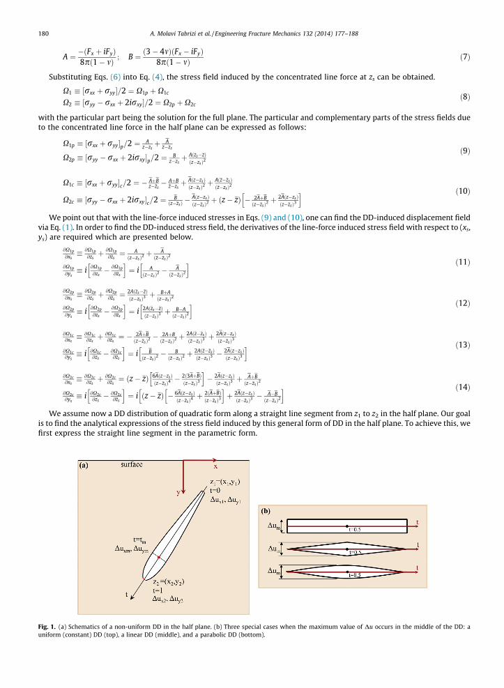
(a) Schematics of a non-uniform DD in the half plane. (b) Three special cases when the maximum value of Du occurs in the middle of the DD: a(constant) DD (top), a linear DD (middle), and a parabolic DD (bottom).

Fig. 2.Crouchhorizon

Table 1Maximuexact cl

N

Max

A. Molavi Tabrizi et al. / Engineering Fracture Mechanics 132 (2014) 177–188 181

x ¼ x1 þ ðx2 � x1Þty ¼ y1 þ ðy2 � y1Þt

ð15Þ

where t = 0 and 1 corresponds to (x,y) = (x1,y1) and (x2,y2), respectively. The length of the DD segment is

L ¼ffiffiffiffiffiffiffiffiffiffiffiffiffiffiffiffiffiffiffiffiffiffiffiffiffiffiffiffiffiffiffiffiffiffiffiffiffiffiffiffiffiffiffiffiffiffiffiffiðx2 � x1Þ2 þ ðy2 � y1Þ

2q

ð16Þ

In terms of the parameter t, the quadratic DD Duj can be assumed as

Duj ¼ 2ðajt2 þ bjt þ cjÞ; j ¼ x; y ð17Þ

where aj, bj, and cj are constants which can be determined from values of Duj at three arbitrary points along the discontinu-ity. In this paper, we consider the start and end points of the discontinuity and a point in between, so that

aj ¼Dujm�tmDuj2þtmDuj1�Duj1

2tmðtm�1Þ

bj ¼Duj2�Duj1

2 � Dujm�tmDuj2þtmDuj1�Duj12tmðtm�1Þ j ¼ x; y

cj ¼Duj1

2

ð18Þ

where Duj1, Dujm, and Duj2 are the magnitudes of the relative displacement at the start (t = 0), at an intermediate point(t = tm), and at the end point (t = 1) of the DD line, respectively. Note that tm varies between 0 and 1, and it does not needto correspond to the point with the maximum value of Duj. One special choice is tm = 0.5 which means that the relative dis-placement Dujm is at the midpoint. Equation (17) represents a general quadratic DD profile as illustrated in Fig. 1a whileFig. 1b shows three special cases where the maximum DD occurs at tm = 0.5 for the uniform (constant), linear, and quadraticdistributions of DD profiles.

Therefore, in terms of parameter t, the DD-induced displacement derivatives can be expressed as follows.

@uk@xs¼ 2npL

R 10

@rkpq

@zsþ @rk

pq

@�zs

h iðaqt2 þ bqt þ cqÞdt

@uk@ys¼ 2npL

R 10 i

@rkpq

@zs� i

@rkpq

@�zs

h iðaqt2 þ bqt þ cqÞdt

k ¼ x; y

p or q ¼ x; y

�ð19Þ

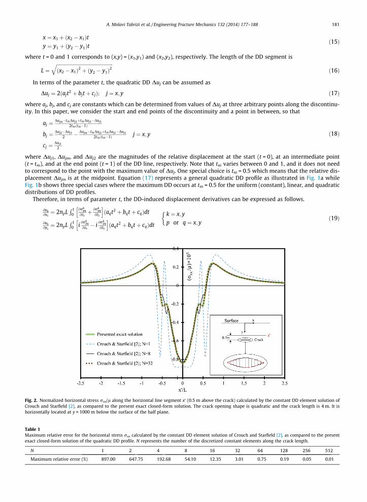
Normalized horizontal stress rxx/l along the horizontal line segment x0 (0.5 m above the crack) calculated by the constant DD element solution ofand Starfield [2], as compared to the present exact closed-form solution. The crack opening shape is quadratic and the crack length is 4 m. It istally located at y = 1000 m below the surface of the half plane.

m relative error for the horizontal stress rxx calculated by the constant DD element solution of Crouch and Starfield [2], as compared to the presentosed-form solution of the quadratic DD profile. N represents the number of the discretized constant elements along the crack length.

1 2 4 8 16 32 64 128 256 512

imum relative error (%) 897.00 647.75 192.68 54.10 12.35 3.01 0.75 0.19 0.05 0.01

182 A. Molavi Tabrizi et al. / Engineering Fracture Mechanics 132 (2014) 177–188

Note that for k = x, we set Fx = 1 and Fy = 0 while for k = y, Fx = 0 and Fy = 1. Thus, in terms of the components, the followingintegrals are needed in order to find the displacement derivatives in Eq. (19).

Fig. 3.The sur

Cmp;xs ¼ 2LR 1

0@Xmp

@xsðajt2 þ bjt þ cjÞdt ¼ 2L

R 10

@Xmp

@zsþ @Xmp

@�zs

h iðajt2 þ bjt þ cjÞdt

Cmp;ys¼ 2L

R 10

@Xmp

@ysðajt2 þ bjt þ cjÞdt ¼ 2iL

R 10

@Xmp

@zs� @Xmp

@�zs

h iðajt2 þ bjt þ cjÞdt

ð20Þ

Cmc;xs ¼ 2LR 1

0@Xmc@xsðajt2 þ bjt þ cjÞdt ¼ 2L

R 10 ½

@Xmc@zsþ @Xmc

@�zs�ðajt2 þ bjt þ cjÞdt

Cmc;ys¼ 2L

R 10

@Xmc@ysðajt2 þ bjt þ cjÞdt ¼ 2iL

R 10

@Xmc@zs� @Xmc

@�zs

h iðajt2 þ bjt þ cjÞdt

ð21Þ

The exact closed-form expressions for the functions Cmp,xs, Cmp,ys, Cmc,xs, and Cmc,ys are given in the Appendix. Using theconstitutive relation in Eq. (3), we can find the corresponding stress field. Note that the particular solution is the full-planesolution and the complementary solution approaches zero far from the surface. As a result, far from the surface the totalsolution approaches the full-plane solution.

3. Numerical examples

For a straight crack in a linear elastic medium, the relative opening displacements generally are non-uniform. Thus, usinga quadratic DD would in many cases yield satisfactory solutions with less discretization and shorter computer runtimes. Toinvestigate the utility of the quadratic DD, we apply our exact closed-form solutions to three DD cases in an isotropic elastichalf plane.

In the first numerical example, we calculate the normal stress field rxx induced by a quadratic DD. Similar to the work byMaerten et al. [25] and Crouch and Starfield [2], in order to approximate the quadratic DD profile, certain numbers ofconstant DD elements are needed. The results illustrated in Fig. 2 consider a horizontal opening-mode DD of length 4 m

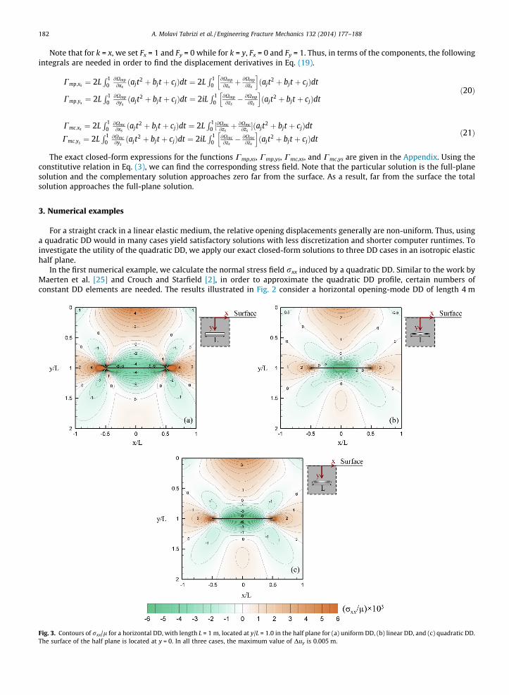
Contours of rxx/l for a horizontal DD, with length L = 1 m, located at y/L = 1.0 in the half plane for (a) uniform DD, (b) linear DD, and (c) quadratic DD.face of the half plane is located at y = 0. In all three cases, the maximum value of Duy is 0.005 m.

A. Molavi Tabrizi et al. / Engineering Fracture Mechanics 132 (2014) 177–188 183

in a half plane. The material properties for the half plane are l = 2 GPa and m = 0.25. The crack is 1000 m below the surface sothat the Crouch and Starfield [2] solution for the constant DD in the full plane can be applied. The DD profile is assumed to bequadratic, with the maximum opening being Duy = 0.005 m at the crack center and zero at its left and right tips. For simplic-ity, the horizontal component of the DD is assumed to be zero along the crack. For this case, our exact closed-form solutionsof the quadratic DD can be directly applied without requiring any discretization. To see the effect of discretization, we havealso applied the constant DD solution of Crouch and Starfield [2] to discretize the quadratic DD profile. Fig. 2 compares thevalues of rxx/l along a line which is 0.5 m above the crack (x0 line). In this figure, the dashed, dotted and thin solid curvescorrespond to the results using the Crouch and Starfield solution [2] with N = 1, 8 and 32 constant DD elements along thewhole length of the crack; the thick solid curve represents the exact closed-form solution of the quadratic DD presentedin this paper. In order to accurately predict the stress field induced by a quadratic DD, 32 constant DD elements are requiredfor a maximum relative error of 3% (Table 1). Table 1 further shows the relative error percentage of using different numbersof elements, as compared to the exact closed-form solutions of quadratic DD profile. For a maximum error less than 1%, 64constant elements are needed, indicating more computational times as compared to the exact closed-form solution pre-sented in this paper.

In the second example, we compare the stress fields of opening-mode DDs with uniform, linear, and quadratic relativedisplacement profiles, respectively. In this example, each horizontal DD line has a length of 1 m located 1 m below the sur-face. Along the DD line, we assume only the relative opening displacements and there is no tangential displacement discon-tinuity (i.e., Dux = 0). Fig. 3a illustrates the contours of the horizontal normal stress rxx induced by the DD where Duy isuniform and equals 0.005 m. Fig. 3b and c shows the contours of the stresses due to the linear and quadratic variations inDuy, with the maximum relative discontinuity being 0.005 m at the crack center and zero at its left and right tips. The mate-rial properties are set to l = 2 GPa and m = 0.25 in each case. The vertical normal stress ryy and shear stress rxy for these threeDD profiles are shown in Figs. 4 and 5, respectively. While Figs. 3–5 each show gross similarities, including a stress singu-larity at the tips of the DD, they differ in detail, especially along the DD. For instance, the stress singularity at the tips is stron-ger for constant DD than for the linear and quadratic ones, and the sign of the near-tip stress perturbation is moreheterogeneous as well. In addition, Fig. 5 demonstrates considerable difference between the shear stress rxy fields induced

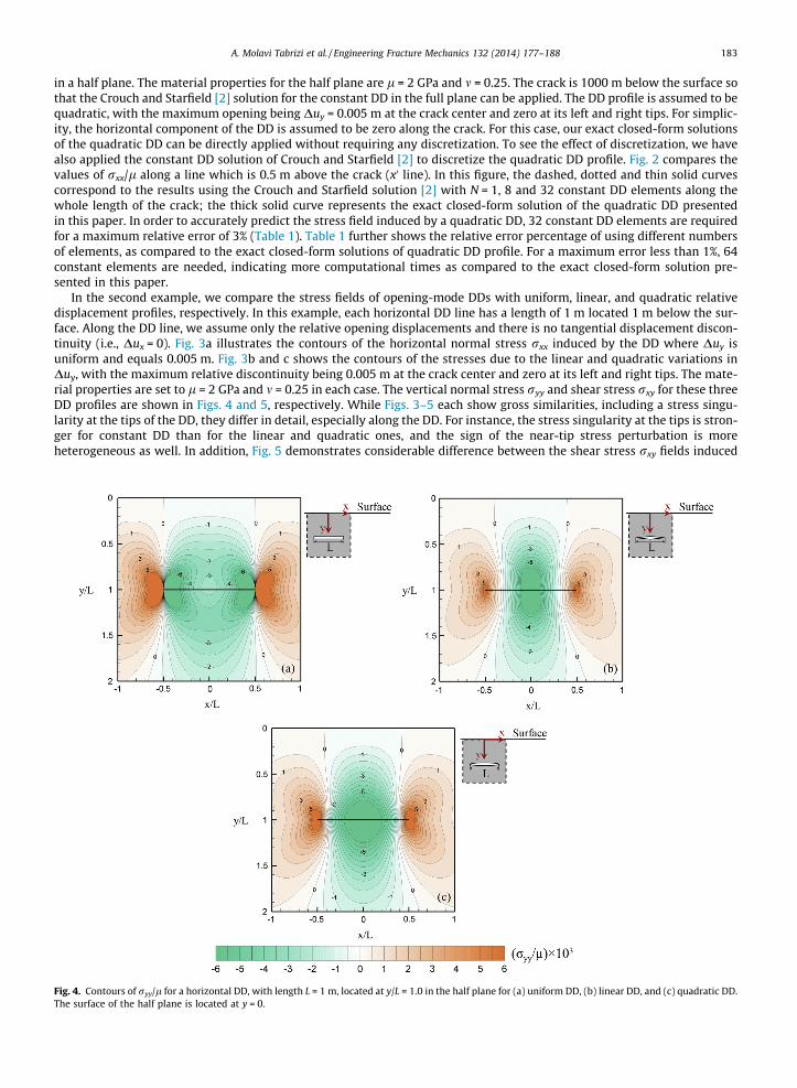
Fig. 4. Contours of ryy/l for a horizontal DD, with length L = 1 m, located at y/L = 1.0 in the half plane for (a) uniform DD, (b) linear DD, and (c) quadratic DD.The surface of the half plane is located at y = 0.

184 A. Molavi Tabrizi et al. / Engineering Fracture Mechanics 132 (2014) 177–188

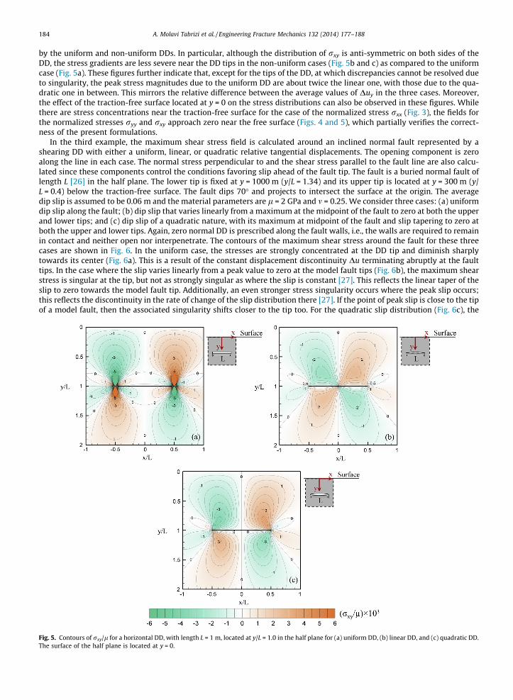
by the uniform and non-uniform DDs. In particular, although the distribution of rxy is anti-symmetric on both sides of theDD, the stress gradients are less severe near the DD tips in the non-uniform cases (Fig. 5b and c) as compared to the uniformcase (Fig. 5a). These figures further indicate that, except for the tips of the DD, at which discrepancies cannot be resolved dueto singularity, the peak stress magnitudes due to the uniform DD are about twice the linear one, with those due to the qua-dratic one in between. This mirrors the relative difference between the average values of Duy in the three cases. Moreover,the effect of the traction-free surface located at y = 0 on the stress distributions can also be observed in these figures. Whilethere are stress concentrations near the traction-free surface for the case of the normalized stress rxx (Fig. 3), the fields forthe normalized stresses ryy and rxy approach zero near the free surface (Figs. 4 and 5), which partially verifies the correct-ness of the present formulations.

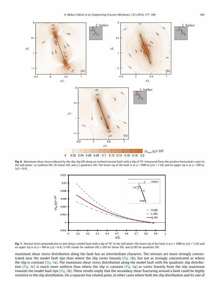
In the third example, the maximum shear stress field is calculated around an inclined normal fault represented by ashearing DD with either a uniform, linear, or quadratic relative tangential displacements. The opening component is zeroalong the line in each case. The normal stress perpendicular to and the shear stress parallel to the fault line are also calcu-lated since these components control the conditions favoring slip ahead of the fault tip. The fault is a buried normal fault oflength L [26] in the half plane. The lower tip is fixed at y = 1000 m (y/L = 1.34) and its upper tip is located at y = 300 m (y/L = 0.4) below the traction-free surface. The fault dips 70� and projects to intersect the surface at the origin. The averagedip slip is assumed to be 0.06 m and the material parameters are l = 2 GPa and m = 0.25. We consider three cases: (a) uniformdip slip along the fault; (b) dip slip that varies linearly from a maximum at the midpoint of the fault to zero at both the upperand lower tips; and (c) dip slip of a quadratic nature, with its maximum at midpoint of the fault and slip tapering to zero atboth the upper and lower tips. Again, zero normal DD is prescribed along the fault walls, i.e., the walls are required to remainin contact and neither open nor interpenetrate. The contours of the maximum shear stress around the fault for these threecases are shown in Fig. 6. In the uniform case, the stresses are strongly concentrated at the DD tip and diminish sharplytowards its center (Fig. 6a). This is a result of the constant displacement discontinuity Du terminating abruptly at the faulttips. In the case where the slip varies linearly from a peak value to zero at the model fault tips (Fig. 6b), the maximum shearstress is singular at the tip, but not as strongly singular as where the slip is constant [27]. This reflects the linear taper of theslip to zero towards the model fault tip. Additionally, an even stronger stress singularity occurs where the peak slip occurs;this reflects the discontinuity in the rate of change of the slip distribution there [27]. If the point of peak slip is close to the tipof a model fault, then the associated singularity shifts closer to the tip too. For the quadratic slip distribution (Fig. 6c), the

Fig. 5. Contours of rxy/l for a horizontal DD, with length L = 1 m, located at y/L = 1.0 in the half plane for (a) uniform DD, (b) linear DD, and (c) quadratic DD.The surface of the half plane is located at y = 0.

Fig. 6. Maximum shear stress induced by the dip-slip DD along an inclined normal fault with a dip of 70� (measured from the positive horizontal x-axis) inthe half plane: (a) uniform DD, (b) linear DD, and (c) quadratic DD. The lower tip of the fault is at y = 1000 m (y/L = 1.34) and its upper tip is at y = 300 m,(y/L = 0.4).

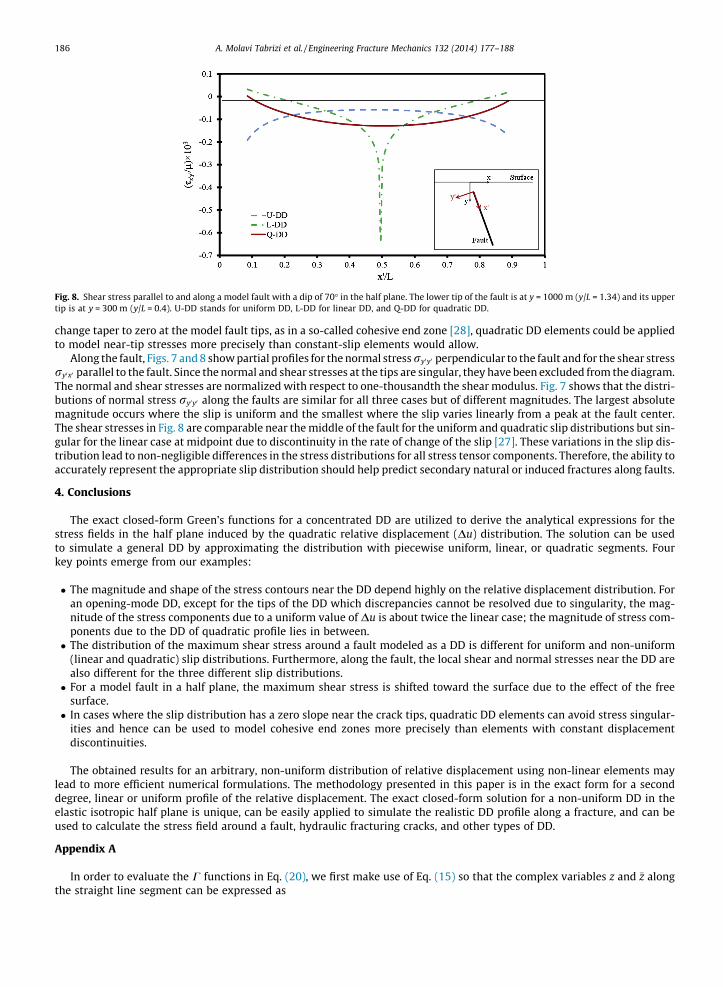
Fig. 7. Normal stress perpendicular to and along a model fault with a dip of 70� in the half plane. The lower tip of the fault is at y = 1000 m (y/L = 1.34) andits upper tip is at y = 300 m (y/L = 0.4). U-DD stands for uniform DD, L-DD for linear DD, and Q-DD for quadratic DD.

A. Molavi Tabrizi et al. / Engineering Fracture Mechanics 132 (2014) 177–188 185

maximum shear stress distribution along the fault has an intermediate character. The stresses are more strongly concen-trated near the model fault tips than where the slip varies linearly (Fig. 6b), but not as strongly concentrated as wherethe slip is constant (Fig. 6a). The maximum shear stress distribution along the model fault with the quadratic slip distribu-tion (Fig. 6c) is much more uniform than where the slip is constant (Fig. 6a) or varies linearly from the slip maximumtowards the model fault tips (Fig. 6b). These results imply that the secondary shear fracturing around a fault could be highlysensitive to the slip distribution. On a separate but related point, in other cases where both the slip distribution and its rate of

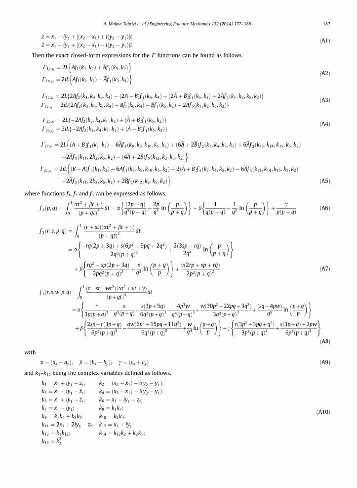
Fig. 8. Shear stress parallel to and along a model fault with a dip of 70� in the half plane. The lower tip of the fault is at y = 1000 m (y/L = 1.34) and its uppertip is at y = 300 m (y/L = 0.4). U-DD stands for uniform DD, L-DD for linear DD, and Q-DD for quadratic DD.

186 A. Molavi Tabrizi et al. / Engineering Fracture Mechanics 132 (2014) 177–188

change taper to zero at the model fault tips, as in a so-called cohesive end zone [28], quadratic DD elements could be appliedto model near-tip stresses more precisely than constant-slip elements would allow.

Along the fault, Figs. 7 and 8 show partial profiles for the normal stress ry0y0 perpendicular to the fault and for the shear stressry0x0 parallel to the fault. Since the normal and shear stresses at the tips are singular, they have been excluded from the diagram.The normal and shear stresses are normalized with respect to one-thousandth the shear modulus. Fig. 7 shows that the distri-butions of normal stress ry0y0 along the faults are similar for all three cases but of different magnitudes. The largest absolutemagnitude occurs where the slip is uniform and the smallest where the slip varies linearly from a peak at the fault center.The shear stresses in Fig. 8 are comparable near the middle of the fault for the uniform and quadratic slip distributions but sin-gular for the linear case at midpoint due to discontinuity in the rate of change of the slip [27]. These variations in the slip dis-tribution lead to non-negligible differences in the stress distributions for all stress tensor components. Therefore, the ability toaccurately represent the appropriate slip distribution should help predict secondary natural or induced fractures along faults.

4. Conclusions

The exact closed-form Green’s functions for a concentrated DD are utilized to derive the analytical expressions for thestress fields in the half plane induced by the quadratic relative displacement (Du) distribution. The solution can be usedto simulate a general DD by approximating the distribution with piecewise uniform, linear, or quadratic segments. Fourkey points emerge from our examples:

� The magnitude and shape of the stress contours near the DD depend highly on the relative displacement distribution. Foran opening-mode DD, except for the tips of the DD which discrepancies cannot be resolved due to singularity, the mag-nitude of the stress components due to a uniform value of Du is about twice the linear case; the magnitude of stress com-ponents due to the DD of quadratic profile lies in between.� The distribution of the maximum shear stress around a fault modeled as a DD is different for uniform and non-uniform

(linear and quadratic) slip distributions. Furthermore, along the fault, the local shear and normal stresses near the DD arealso different for the three different slip distributions.� For a model fault in a half plane, the maximum shear stress is shifted toward the surface due to the effect of the free

surface.� In cases where the slip distribution has a zero slope near the crack tips, quadratic DD elements can avoid stress singular-

ities and hence can be used to model cohesive end zones more precisely than elements with constant displacementdiscontinuities.

The obtained results for an arbitrary, non-uniform distribution of relative displacement using non-linear elements maylead to more efficient numerical formulations. The methodology presented in this paper is in the exact form for a seconddegree, linear or uniform profile of the relative displacement. The exact closed-form solution for a non-uniform DD in theelastic isotropic half plane is unique, can be easily applied to simulate the realistic DD profile along a fracture, and can beused to calculate the stress field around a fault, hydraulic fracturing cracks, and other types of DD.

Appendix A

In order to evaluate the C functions in Eq. (20), we first make use of Eq. (15) so that the complex variables z and �z alongthe straight line segment can be expressed as

A. Molavi Tabrizi et al. / Engineering Fracture Mechanics 132 (2014) 177–188 187

z ¼ x1 þ iy1 þ ½ðx2 � x1Þ þ iðy2 � y1Þ�t�z ¼ x1 � iy1 þ ½ðx2 � x1Þ � iðy2 � y1Þ�t

ðA1Þ

Then the exact closed-form expressions for the C functions can be found as follows.

C1p;xs ¼ 2L Af1ðk1; k2Þ þ Af 1ðk3; k4Þn o

C1p;ys¼ 2iL Af1ðk1; k2Þ � Af 1ðk3; k4Þ

n o ðA2Þ

C1c;xs ¼ 2Lf2Af2ðk3; k4; k6; k4Þ � ð2Aþ BÞf 1ðk6; k4Þ � ð2Aþ BÞf 1ðk5; k2Þ þ 2Af 2ðk1; k2; k5; k2ÞgC1c;ys

¼ 2iLf2Af2ðk3; k4; k6; k4Þ � Bf1ðk6; k4Þ þ Bf 1ðk5; k2Þ � 2Af 2ðk1; k2; k5; k2ÞgðA3Þ

C2p;xs ¼ 2Lf�2Af2ðk3; k4; k1; k2Þ þ ðAþ BÞf 1ðk5; k2ÞgC2p;ys

¼ 2iLf�2Af2ðk3; k4; k1; k2Þ þ ðA� BÞf 1ðk5; k2ÞgðA4Þ

C2c;xs ¼ 2L ðAþ BÞf 1ðk1; k2Þ � 6Af 3ðk8; k9; k10; k5; k2Þ þ ð6Aþ 2BÞf 2ðk7; k4; k5; k2Þ þ 6Af 3ðk13; k14; k15; k5; k2Þn�2Af 2ðk11;2k2; k5; k2Þ � ð4Aþ 2BÞf 2ðk12; k2; k5; k2Þ

oC2c;ys

¼ 2iL ðB� AÞf 1ðk1; k2Þ þ 6Af 3ðk8; k9; k10; k5; k2Þ � 2ðAþ BÞf 2ðk7; k4; k5; k2Þ � 6Af 3ðk13; k14; k15; k5; k2Þnþ2Af 2ðk11;2k2; k5; k2Þ þ 2Bf 2ðk12; k2; k5; k2Þ

oðA5Þ

where functions f1, f2 and f3 can be expressed as follows.

f 1ðp; qÞ ¼Z 1

0

at2 þ bt þ cðpþ qtÞ2

dt ¼ að2pþ qÞq2ðpþ qÞ þ

2pq3 ln

ppþ q

� �� �� b

1qðpþ qÞ þ

1q2 ln

ppþ q

� �� �þ c

pðpþ qÞ ðA6Þ

f 2ðr; s; p; qÞ ¼Z 1

0

ðr þ stÞðat2 þ bt þ cÞðpþ qtÞ3

dt

¼ a�rqð2pþ 3qÞ þ sð6p2 þ 9pqþ 2q2Þ

2q3ðpþ qÞ2þ 2ð3sp� rqÞ

2q4 lnp

pþ q

� �( )

þ brq2 � spð2pþ 3qÞ

2pq2ðpþ qÞ2þ s

q3 lnpþ q

p

� �( )þ cð2rpþ spþ rqÞ

2p2ðpþ qÞ2ðA7Þ

f 3ðr;s;w;p;qÞ¼Z 1

0

ðrþ stþwt2Þðat2þbtþcÞðpþqtÞ4

dt

¼ar

3pðpþqÞ3� s

q3ðpþqÞ�sð3pþ5qÞ6q2ðpþqÞ3

þ 4p3w

q4ðpþqÞ3þwð30p2þ22pqþ3q2Þ

3q3ðpþqÞ3þðsq�4pwÞ

q5 lnpþq

p

� �( )

þb2spþ rð3pþqÞ

6p2ðpþqÞ3�qwð6p2þ15pqþ11q2Þ

6q4ðpþqÞ3þw

q4 lnpþq

p

� �( )þc

rð3p2þ3pqþq2Þ3p3ðpþqÞ3

þ sð3pþqÞþ2pw

6p2ðpþqÞ3

( )

ðA8Þ

with

a ¼ ðax þ ayÞ; b ¼ ðbx þ byÞ; c ¼ ðcx þ cyÞ ðA9Þ

and k1–k15 being the complex variables defined as follows.

k1 ¼ x1 þ iy1 � zs; k2 ¼ ðx2 � x1Þ þ iðy2 � y1Þ;k3 ¼ x1 � iy1 � �zs; k4 ¼ ðx2 � x1Þ � iðy2 � y1Þ;k5 ¼ x1 þ iy1 � �zs; k6 ¼ x1 � iy1 � zs;

k7 ¼ x1 � iy1; k8 ¼ k1k7;

k9 ¼ k1k4 þ k2k7; k10 ¼ k2k4;

k11 ¼ 2x1 þ 2iy1 � zs; k12 ¼ x1 þ iy1;

k13 ¼ k1k12; k14 ¼ k12k2 þ k2k1;

k15 ¼ k22

ðA10Þ

188 A. Molavi Tabrizi et al. / Engineering Fracture Mechanics 132 (2014) 177–188

References

[1] Crouch S. Solution of plane elasticity problems by the displacement discontinuity method. I. Infinite body solution. Int J Numer Meth Engng1976;10:301–43.

[2] Crouch S, Starfield A. Boundary element methods in solid mechanics. London: Allen and Unwin; 1983.[3] Shou K, Crouch S. A higher order displacement discontinuity method for analysis of crack problems. Int J Rock Mech Min Sci Geomech

1995;32(1):49–55.[4] Fares N, Li VC. An indirect boundary element method for 2-D finite/infinite regions with multiple displacement discontinuities. Engng Fract Mech

1987;26:127–41.[5] Pan E, Amadei B. Fracture mechanics analysis of cracked 2-D anisotropic media with a new formulation of the boundary element method. Int J Fract

1996;77:161–74.[6] Pan E. A general boundary element analysis of 2-D linear elastic fracture mechanics. Int J Fract 1997;88:41–59.[7] Pan E, Yuan F. Boundary element analysis of three-dimensional cracks in anisotropic solids. Int J Numer Meth Engng 2000;48:211–37.[8] Azhdari A, Obata M, Nemat-Nasser S. Alternative solution methods for crack problems in plane anisotropic elasticity, with examples. Int J Solids Struct

2000;37:6433–78.[9] Hossaini Nasab H, Marji MF. A semi-infinite higher-order displacement discontinuity method and its application to the quasistatic analysis of radial

cracks produced by blasting. Mech Mater Struct 2007;2(3):439–57.[10] Ma G, An X, Zhang H, Li L. Modeling complex crack problems using the numerical manifold method. Int J Fract 2009;156:21–35.[11] Zhang H, Li L, An X, Ma G. Numerical analysis of 2-D crack propagation problems using the numerical manifold method. Engng Anal Boundary Elem

2010;34:41–50.[12] Kübbeler M, Roth I, Krupp U, Fritzen CP, Christ HJ. Simulation of stage I-crack growth using a hybrid boundary element technique. Engng Fract Mech

2011;78:462–8.[13] Gordeliy E, Piccinin R, Napier JA, Detournay E. Axisymmetric benchmark solutions in fracture mechanics. Engng Fract Mech 2013;102:348–57.[14] d’Alessio M, Martel SJ. Development of strike slip faults from dikes, Sequoia National Park, California. J Struct Geol 2005;27:35–49.[15] Maerten L, Willemse EJ, Pollard DD, Rawnsley K. Slip distributions on intersecting normal faults. J Struct Geol 1999;21:259–72.[16] Maerten L, Gillespie P, Pollard DD. Effects of local stress perturbation on secondary fault development. J Struct Geol 2002;24:145–53.[17] Meng C, Maerten F, Pollard DD. Modeling mixed-mode fracture propagation in isotropic elastic three dimensional solid. Int J Fract 2013;179(1–

2):45–57.[18] Martel SJ. Modeling elastic stresses in long ridges with the displacement discontinuity method. Pure Appl Geophys 2000;157:1039–57.[19] Muller J, Martel SJ. Numerical models of translational landslide rupture surface growth. Pure Appl Geophys 2000;157:1009–38.[20] Martel SJ. Mechanics of landslide initiation as a shear fracture phenomenon. Mar Geol 2004;203:319–39.[21] Soliva R, Maerten F, Petit JP, Auzias V. Field evidences for the role of static friction on fracture orientation in extensional relays along strike-slip faults:

comparison with photoelasticity and 3-D numerical modeling. J Struct Geol 2010;32(11):1721–31.[22] Pan E. Dislocation in an infinite poroelastic medium. Acta Mech 1991;87(1–2):105–15.[23] Timoshenko S, Goodier JN. Theory of elasticity. 3rd ed. New York: Mc Graw-Hill Book Company; 1953.[24] Muskhelishvili N. Some basic problems of the mathematical theory of elasticity: fundamental equations, plane theory of elasticity, torsion and

bending. 3rd ed. Leiden: Noordhoff International Publishing; 1953.[25] Maerten F, Maerten L, Cooke M. Solving 3D boundary element problems using constrained iterative approach. Comput Geosci 2010;14(4):551–64.[26] Martel SJ, Langley JS. Propagation of normal faults to the surface in basalt, Koae fault system, Hawaii. J Struct Geol 2006;28:2123–43.[27] Martel SJ, Shacat C. Mechanics and interpretations of fault slip. In: Earthquakes: Radiated Energy and the Physics of Faulting; 2006. p. 207–15.[28] Martel SJ. Effects of cohesive zones on small faults and implications for secondary fracturing and fault trace geometry. J Struct Geol

1997;19(6):835–47.