Page 1
Engineering the Implementation of Pumped Hydro
Energy Storage in the Arizona Power Grid
by
William Jesse J. Dixon
A Thesis Presented in Partial Fulfillment
of the Requirements for the Degree
Master of Science
Approved November 2014 by
the Graduate Supervisory Committee:
Gerald Heydt, Chair
Kory Hedman
George Karady
ARIZONA STATE UNIVERSITY
December 2014
Page 2
i
ABSTRACT
This thesis addresses the issue of making an economic case for bulk energy storage in the
Arizona bulk power system. Pumped hydro energy storage (PHES) is used in this study. Bulk
energy storage has often been suggested for large scale electric power systems in order to levelize
load (store energy when it is inexpensive [energy demand is low] and discharge energy when it is
expensive [energy demand is high]). It also has the potential to provide opportunities to avoid
transmission and generation expansion, and provide for generation reserve margins. As the level
of renewable energy resources increases, the uncertainty and variability of wind and solar
resources may be improved by bulk energy storage technologies.
For this study, the MATLab software platform is used, a mathematical based modeling
language, optimization solvers (specifically Gurobi), and a power flow solver (PowerWorld) are
used to simulate an economic dispatch problem that includes energy storage and transmission
losses. A program is created which utilizes quadratic programming to analyze various cases using
a 2010 summer peak load from the Arizona portion of the Western Electricity Coordinating
Council (WECC) system. Actual data from industry are used in this test bed. In this thesis, the full
capabilities of Gurobi are not utilized (e.g., integer variables, binary variables). However, the
formulation shown here does create a platform such that future, more sophisticated modeling may
readily be incorporated.
The developed software is used to assess the Arizona test bed with a low level of energy storage
to study how the storage power limit effects several optimization outputs such as the system wide
operating costs. Large levels of energy storage are then added to see how high level energy storage
affects peak shaving, load factor, and other system applications. Finally, various constraint
relaxations are made to analyze why the applications tested eventually approach a constant value.
Page 3
ii
This research illustrates the use of energy storage which helps minimize the system wide generator
operating cost by “shaving” energy off of the peak demand.
The thesis builds on the work of another recent researcher with the objectives of strengthening
the assumptions used, checking the solutions obtained, utilizing higher level simulation languages
to affirm results, and expanding the results and conclusions.
One important point not fully discussed in the present thesis is the impact of efficiency in the
pumped hydro cycle. The efficiency of the cycle for modern units is estimated at higher than 90%.
Inclusion of pumped hydro losses is relegated to future work.
Page 4
iii
ACKNOWLEDGEMENTS
I would like to share my sincere gratitude to my advisor, Dr. Gerald T. Heydt, for his
continuous support of my thesis, his patience, positive attitude, incredible wisdom, and guidance.
Without his motivation and enthusiasm, the completion of this thesis would not have been possible.
I could not have asked for a better advisor and mentor for my thesis and I am forever thankful and
in his debt. I would also like to thank Dr. Kory Hedman and Dr. George Karady for offering their
time and effort to be a part of my graduate supervisory committee.
I would like to acknowledge the Power Systems Engineering Research Center (PSERC), a
National Science Foundation ‘Industry – University Cooperative Research Center’ for their
financial assistance. The NSF center is a Generation III Engineering Research Center supported
by industry and the U.S. National Science Foundation under grant EEC-0968993.
Page 5
iv
TABLE OF CONTENTS
.......................................................................................................................................................... Page
LIST OF FIGURES .............................................................................................................................. vii
LIST OF TABLES ................................................................................................................................ ix
NOMENCLATURE .............................................................................................................................. xi
CHAPTER
1 OBJECTIVES RELATING TO PUMPED HYDRO ENERGY STORAGE IN POWER
TRANSMISSION SYSTEMS................................................................................................................ 1
1.1 Bulk Energy Storage in Arizona .................................................................................................. 1
1.2 Motivation for this Thesis ............................................................................................................ 1
1.3 Bulk Energy Storage Applications ............................................................................................... 2
Peak Shaving/Load Leveling .................................................................................................. 2
Transmission Expansion Deferral ......................................................................................... 3
Incorporating Renewable Energy Technology ...................................................................... 5
1.4 Bulk Energy Storage Technology - Pumped Hydro Energy Storage (PHES) ............................. 6
1.5 Optimization Method ................................................................................................................... 7
Economic Dispatch ................................................................................................................ 7
Economic Dispatch for a Thermal Unit Example .................................................................. 8
1.6 Organization of this Thesis ........................................................................................................ 10
2 TECHNICAL THEORETICAL BASIS OF BULK ENERGY STORAGE ..................................... 11
2.1 Large Scale (Bulk) Energy Storage in Power Systems .............................................................. 11
2.2 Economic Dispatch Methodology .............................................................................................. 11
2.3 Formulation of the Bulk Energy Storage Problem ..................................................................... 13
2.4 Problem Formulation Assumptions ........................................................................................... 17
Page 6
v
CHAPTER Page
2.5 Incorporating Transmission Line Losses ................................................................................... 18
An Alternative for the Incorporation of Transmission Line Losses ..................................... 21
3 APPLICATION OF BULK ENERGY STORAGE IN ARIZONA .................................................. 24
3.1 Description of the Arizona Test Bed.......................................................................................... 24
3.2 PHES Facility Locations ............................................................................................................ 26
Theoretical and Hypothetical PHES Locations ................................................................... 26
Currently Planned and Potential Future PHES Locations .................................................. 27
Longview Energy Exchange ................................................................................................. 28
Table Mountain Hydro ......................................................................................................... 29
3.3 Description of Test Cases .......................................................................................................... 29
3.4 Arizona Base Case – Summer 2010 ........................................................................................... 31
3.5 Arizona Pumped Hydro Energy Storage Cases ......................................................................... 32
3.5 Payback Period Calculation ....................................................................................................... 34
3.6 Summary of the Results ............................................................................................................. 37
Case 1 – E/P = 1, Unaltered Generator Cost Curves ............................................................... 37
Case 4 – E/P = 5, Unaltered Generator Cost Curves ............................................................... 39
Case 7 – E/P = 10, Unaltered Generator Cost Curves ............................................................. 41
3.7 Conclusions ................................................................................................................................ 43
4 SENSITIVITY STUDY OF GENERATION COSTS ...................................................................... 44
4.1 Deviation of Generator Cost Curves .......................................................................................... 44
4.2 Description of Sensitivity Study Cases ...................................................................................... 45
4.3 Sensitivity Study Results ........................................................................................................... 46
5 CONCLUSIONS AND FUTURE WORK ........................................................................................ 50
Page 7
vi
CHAPTER Page
5.1 Conclusions ................................................................................................................................ 50
5.2 Future Work ............................................................................................................................... 54
REFERENCES ..................................................................................................................................... 56
APPENDIX
A MATLAB CODE ............................................................................................................................. 59
A.1 MATLab Code: Formulate and Solve the Economic Dispatch for the Annual Cost ................ 60
A.2 MATLab Code: Extrapolate Generator Data and Export into a Form Usable by PowerWorld 69
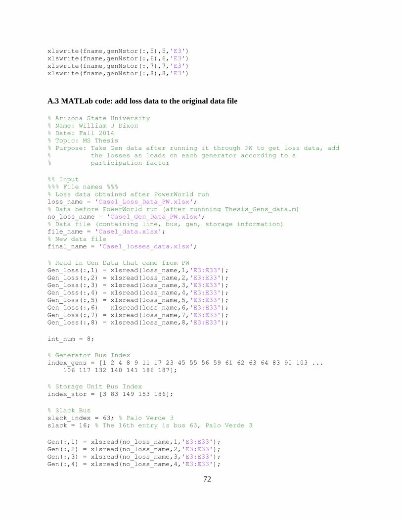
A.3 MATLab Code: Add Loss Data to the Original Data File ........................................................ 72
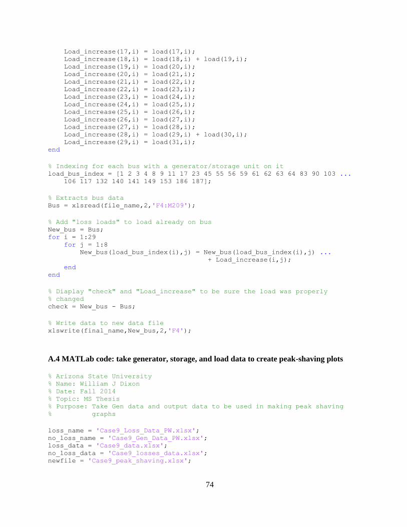
A.4 MATLab Code: Take Generator, Storage, and Load Data to Create Peak-Shaving Plots ........ 74
B CASE SPECIFIC PEAK-SHAVING DATA ................................................................................... 77
B.1 Peak-Shaving Data .................................................................................................................... 78
C GUROBI OPTIMIZER ..................................................................................................................... 85
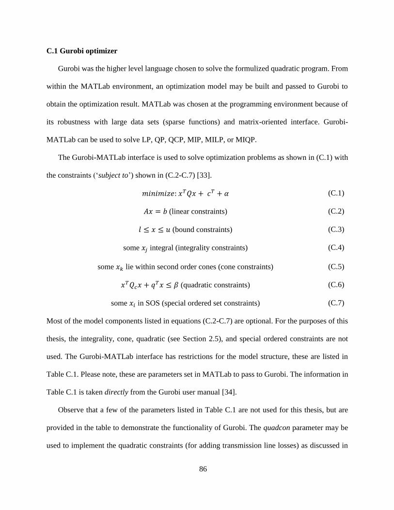
C.1 Gurobi Optimizer ...................................................................................................................... 86
Page 8
vii
LIST OF FIGURES
Figure Page
1.1 Peak Shaving General Diagram ........................................................................................................ 2
1.2 Load Leveling General Diagram ...................................................................................................... 3
1.3 A Simple PHES Facility Diagram .................................................................................................... 6
1.4 Simple Economic Dispatch Problem ................................................................................................ 8
1.5 Thermal Generator Unit Operating Cost Curve ............................................................................... 9
2.1 DC, lossless, lumped parameter transmission line model, used for power flow analysis .............. 20
3.1 Diagram of Concept of Adding PHES to Economic Dispatch Problem ........................................ 24
3.2 Arizona 2010 Summer Peak – Heavy Load Approximation using Piecewise Linear Segments ... 26
3.3 Arizona Map with PHES Locations ............................................................................................... 30
3.4 Case 1 - Lossless Peak-Shaving ..................................................................................................... 38
3.5 Case 1 – Losses Included Peak-Shaving ........................................................................................ 38
3.6 Case 4 – Lossless Peak-Shaving ..................................................................................................... 40
3.7 Case 4 – Losses Included Peak-Shaving ........................................................................................ 40
3.8 Case 7 – Lossless Peak-Shaving ..................................................................................................... 42
3.9 Case 7 – Losses Included Peak-Shaving ........................................................................................ 42
B.1: Case 1 – Lossless Peak-Shaving ................................................................................................... 78
B.2: Case 1 – Losses Included Peak-Shaving ...................................................................................... 79
B.3: Case 2 – Lossless Peak-Shaving ................................................................................................... 79
B.4: Case 2 – Losses Included Peak-Shaving ...................................................................................... 79
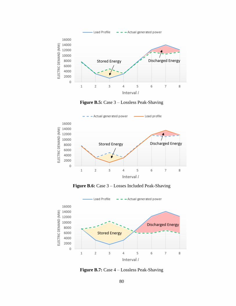
B.5: Case 3 – Lossless Peak-Shaving ................................................................................................... 80
B.6: Case 3 – Losses Included Peak-Shaving ...................................................................................... 80
B.7: Case 4 – Lossless Peak-Shaving ................................................................................................... 80
B.8: Case 4 – Losses Included Peak-Shaving ...................................................................................... 81
B.9: Case 5 – Lossless Peak-Shaving ................................................................................................... 81
Page 9
viii
Figure Page
B.10: Case 5 – Losses Included Peak-Shaving..................................................................................... 81
B.11: Case 6 – Lossless Peak-Shaving ................................................................................................. 82
B.12: Case 6 – Losses Included Peak-Shaving..................................................................................... 82
B.13: Case 7 – Lossless Peak-Shaving ................................................................................................. 82
B.14: Case 7 – Losses Included Peak-Shaving..................................................................................... 83
B.15: Case 8 – Lossless Peak-Shaving ................................................................................................. 83
B.16: Case 8 – Losses Included Peak-Shaving..................................................................................... 83
B.17: Case 9 – Lossless Peak-Shaving ................................................................................................. 84
B.18: Case 9 – Losses Included Peak-Shaving..................................................................................... 84
Page 10
ix
LIST OF TABLES
Table Page
2.1 Generator Cost Coefficients ........................................................................................................... 13
2.2 Simplified Cost Curve Coefficients ................................................................................................ 14
2.3 Assumptions used in Ruggiero Thesis ........................................................................................... 17
2.4 Assumptions used in this Thesis ..................................................................................................... 18
2.5 Assumptions made in PowerWorld ................................................................................................ 22
3.1 Test Bed Assumptions for this Thesis ............................................................................................ 25
3.2 System Profile: an Equivalenced System used for this Thesis ....................................................... 26
3.3 Theoretical PHES Projects ............................................................................................................. 27
3.4 Future Planned PHES Projects ....................................................................................................... 28
3.5 Simulated PHES Location Specific Information ............................................................................ 31
3.6 Case Numbering System ................................................................................................................ 33
3.7 Power and Energy Ratings of Selected PHES in the U.S. .............................................................. 33
3.8 PHES Case Scenarios ..................................................................................................................... 34
3.9 Assumed PHES Capital Costs ........................................................................................................ 35
3.10 PHES Facility Initial Investment Costs for Each Case ................................................................. 36
4.1 Simplified Cost Curve Coefficients Varied by +10% .................................................................... 45
4.2 Simplified Cost Curve Coefficients Varied by -10% ..................................................................... 45
4.3 Calculated System Annual Operating Costs (no Transmission Losses) ......................................... 47
4.4 Calculated System Annual Operating Costs (with Transmission Losses) ...................................... 47
4.5 Calculated System Annual Savings from Adding PHES (no Transmission Losses) ..................... 47
4.6 Calculated System Annual Savings from Adding PHES (with Transmission Losses) .................. 48
4.7 Minimum Payback Period (no Transmission Losses) .................................................................... 48
4.8 Minimum Payback Period (with Transmission Losses) ................................................................. 48
4.9 Maximum Payback Period (no Transmission Losses) ................................................................... 49
Page 11
x
Table Page
4.10 Maximum Payback Period (with Transmission Losses) .............................................................. 49
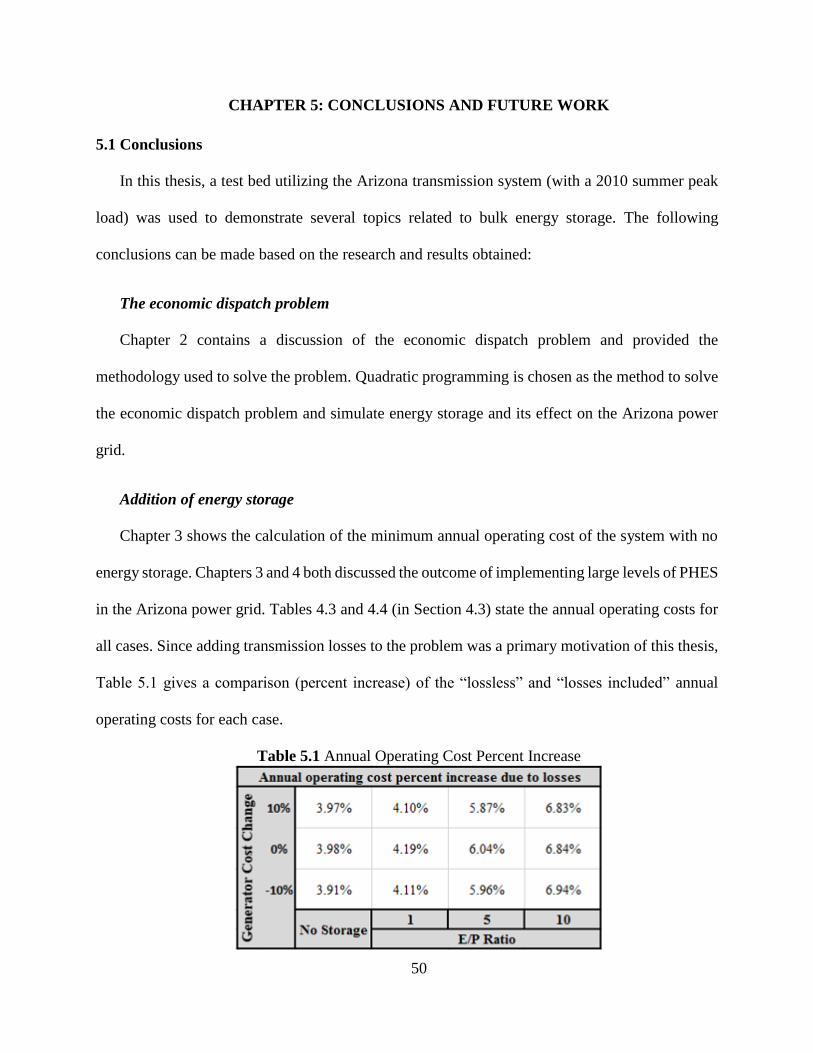
5.1 Annual Operating Cost Percent Increase ........................................................................................ 50
5.2 Best Case (Cheapest Storage Costs) Payback Period Percent Increase .......................................... 51
5.3 Worst Case (Most Expensive Storage Costs) Payback Period Percent Increase ............................ 51
5.4 Percent Increase of Annual Operating Cost from Deviating the Generator Costs ......................... 52
5.5 Percent Increase of Annual Operating Cost from Deviating the Generator Costs ......................... 52
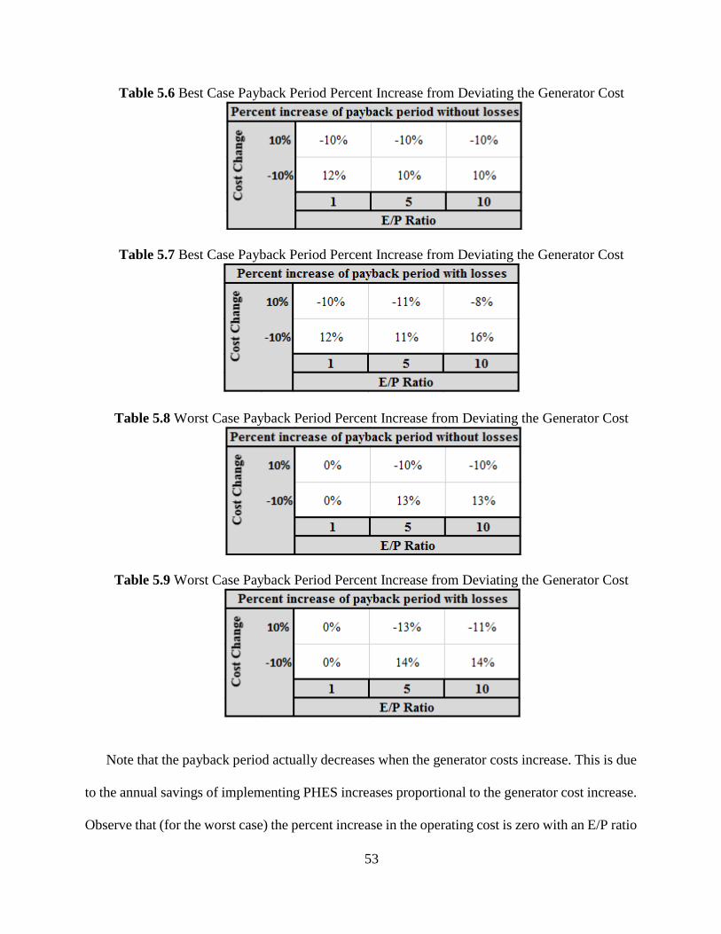
5.6 Best Case Payback Period Percent Increase from Deviating the Generator Cost .......................... 53
5.7 Best Case Payback Period Percent Increase from Deviating the Generator Cost .......................... 53
5.8 Worst Case Payback Period Percent Increase from Deviating the Generator Cost ........................ 53
5.9 Worst Case Payback Period Percent Increase from Deviating the Generator Cost ........................ 53
C.1 Gurobi-MATLab Interface Argument Descriptions ...................................................................... 87
Page 12
xi
NOMENCLATURE
a Quadratic Coefficient of the Approximation for the Cost of Generation
A Coefficient Matrix (m x n) of Inequality Constraints
A Uniform Amount per Interest Period
Aeq Coefficient Matrix (k x n) of Equality Constraints
Aquad Coefficient Matrix (j x n) of Quadratic Constraints
b Linear Coefficient of the Approximation for the Cost of Generation
b Vector (m x 1) of Inequality Right-Hand Side Constraints
beq Vector (k x 1) of Inequality Right-Hand Side Constraints
bquad Vector (j x 1) of Quadratic Right-Hand Side Constraints
Bk Susceptance of Transmission Element k
c No Load Coefficient of the Approximation for the Cost of Generation
c Coefficient of the Cost Function of Generator g
CT Combined Cycle Power Plant
Cg Linear Coefficient, b, of the Cost Function of Generator g
ED Economic Dispatch
E/P Ratio of Maximum Energy Stored in a Pumped Hydro Energy Storage Facility to
the Maximum Power (Rated Power). E is Usually in MWh and P in MW.
EPAct Energy Policy Act
Es Energy Stored in Storage Unit s in MWh
Es,max Maximum Energy Capacity of Storage Unit s in MWh
ET Total Energy Supplied in MWh
Fc Generator Fuel Cost in $/MBTU
Page 13
xii
g Generator Unit
GT Gas Turbine
i Interval Number (1, 2, 3, …, 8)
i Interest Rate per Interest Period
k(.,n) Set of Transmission Assets with n as the “From” Node
k(n,.) Set of Transmission Assets with n at the “To” Node
l Vector of Lower Bound Variables
LP Linear Programming
m,n Bus Number (Nodes)
MIP Mixed Integer Programming
MILP Mixed Integer Linear Programming
MIQCP Mixed Integer Quadratic Constraint Programming
MIQP Mixed Integer Quadratic Programming
n Number of Compounding Periods, or Expected Life of an Asset
P Present Worth, Value, or Amount
Pg Real Power Output of Generator g in MW
Pg,max Maximum Power Capacity of Generator g in MW
Pg,min Minimum Power Capacity of Generator g in MW
PHES Pumped Hydro Energy Storage
Pk Power Flow of Transmission Line k in MW
Pk,max Maximum Line Flow Rating of Transmission Element k in MW
Pl Active Power of Load l in MW
Page 14
xiii
Ppeak Peak Power Demand in MW
Ps Real Power Output of Storage Unit s in MW
Ps,max Maximum Power Capacity of Storage Unit s in MW
Ps,min Minimum Power Capacity of Storage Unit s in MW
PV Photovoltaic
Qg Quadratic Coefficient, a, of the Cost Function of Generator g
QCP Quadratic Constrained Programming
QP Quadratic Programming
Rg Ramp Rate Limit of Generator g in MW/h
RPS Renewable Portfolio Standard
s Storage Unit
SRP Salt River Project
ST Steam Turbine
T Time Period in Hours
u Vector of Upper Bound Variables
OM Generator Operation and Maintenance Costs in $/MWh
WAPA Western Area Power Administration
WECC Western Electricity Coordinating Council
x Vector of Generated System Variable Outputs
xj Variables that must be Integers
δk Bus Voltage Angle at Bus (Node) k
∆t Length of the Time Interval i in Hours
Page 15
1
CHAPTER 1: OBJECTIVES RELATING TO PUMPED HYDRO ENERGY
STORAGE IN POWER TRANSMISSION SYSTEMS
1.1 Bulk energy storage in Arizona
This research addresses a detailed investigation into the economic justification for bulk energy
storage while considering multiple goals which include cost, congestion, and peak shaving for
increasing levels of renewable resource penetration. The research specifically uses pumped hydro
energy storage (PHES) as the means for bulk energy storage. The test bed used is the Arizona
electric power transmission system.
1.2 Motivation for this thesis
A previous study was conducted in 2013 on energy storage for Arizona by Master’s candidate
John Ruggiero [1]. While the study showed that it was economically feasible to implement PHES
into the Arizona grid, many technical assumptions were made. The present thesis focuses on many
of those assumptions, and works to make improvements in order to increase the accuracy of the
results. A sensitivity study of the results on various assumptions is given. In particular, research
objectives for this work include:
strengthening the assumptions used
checking the solutions obtained
utilizing higher level simulation languages to affirm results
expanding the results and conclusions.
Page 16
2
1.3 Bulk energy storage applications
Peak shaving/load leveling
PHES can be used as the means of which to perform peak shaving and load leveling. Peak
shaving and load leveling are methods which utilize energy storage in an economic way (in order
to save money and resources) by reducing the amount of generation used during high demand
hours [2]. For example, electrical energy would be stored when the electrical load is low (cost is
low) and discharged when the electrical load is high (cost is high). By doing so, an entity may be
able to save money by storing energy (excess generation) when the demand is low and discharging
said energy when the demand is high [3].
Peak shaving stores energy during a time in which the system load is low and discharged to
remove only the peaks of the load. Peak shaving eliminates the need to use generation from
peaking power plants (power plants used only during peak hours). For most load profiles, the
system demand is low during morning hours and high in the evening (peak hours). Peak shaving
allows generation to be higher in the morning hours, storing the excess generation. This stored
energy is then discharged during peak hours so that the peak load is in effect reduced. Figure 1.1
illustrates this idea.
Figure 1.1 Peak Shaving General Diagram
Page 17
3
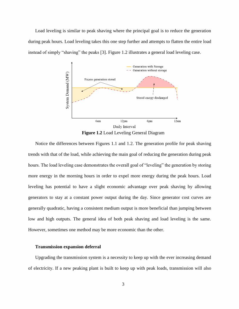
Load leveling is similar to peak shaving where the principal goal is to reduce the generation
during peak hours. Load leveling takes this one step further and attempts to flatten the entire load
instead of simply “shaving” the peaks [3]. Figure 1.2 illustrates a general load leveling case.
Figure 1.2 Load Leveling General Diagram
Notice the differences between Figures 1.1 and 1.2. The generation profile for peak shaving
trends with that of the load, while achieving the main goal of reducing the generation during peak
hours. The load leveling case demonstrates the overall goal of “leveling” the generation by storing
more energy in the morning hours in order to expel more energy during the peak hours. Load
leveling has potential to have a slight economic advantage over peak shaving by allowing
generators to stay at a constant power output during the day. Since generator cost curves are
generally quadratic, having a consistent medium output is more beneficial than jumping between
low and high outputs. The general idea of both peak shaving and load leveling is the same.
However, sometimes one method may be more economic than the other.
Transmission expansion deferral
Upgrading the transmission system is a necessity to keep up with the ever increasing demand
of electricity. If a new peaking plant is built to keep up with peak loads, transmission will also
Page 18
4
need to be built to support that new power plant. Another benefit to incorporating energy storage
into a grid is the ability to defer or eliminate transmission (and distribution) expansion [4]. A few
of these benefits are briefly described below [5].
Deferred transmission and distribution upgrade investment: A single year
transmission or distribution deferral benefit is the financial value associated with
deferring a utility transmission and distribution upgrade for one year. Essentially, the
financial carrying charges are avoided because the upgrade was deferred instead of
immediately taken. The savings may be used to finance energy storage support, which
later on will accumulate savings on its own.
Transmission and distribution equipment life extension: This is similar to that of a
transmission deferral. Use of energy storage reduces the maximum load or load swings
on transmission and distribution equipment. Essentially this results in an extension of
the equipment’s life, the magnitude of the benefit is roughly the same as that of a
transmission deferral.
Transmission support: Energy storage has the potential to improve the performance
of the transmission system. Energy storage support increases the load carrying capacity
of the transmission system (at any location). An accumulated benefit occurs if
additional load carrying capacity defers the need to add more transmission or
equipment.
Avoid transmission access charges: If a utility does not own transmission lines that
are utilized to delivery energy to a customer, they pay the owners of said transmission
lines for transmission “service”. These charges are called transmission access charges.
Page 19
5
Reduced cost for line losses: In most cases, a differential exists between transmission
and distribution resistive losses during on and off peak hours. In a purely hypothetical
example, if the resistive losses are 10% during peak hours and 6% off peak hours, the
avoided losses from implementing storage could be 4% (as long as the storage is
located in a reasonably close geographical distance). In effect, this reduces generator
fuel consumption and the need for generation and transmission expansion.
Incorporating renewable energy technology
Many of the US states have initiated renewable portfolio standards (RPS) in order to push the
development of renewable energy into their systems. Specifically, Arizona’s RPS requires that
15% of all its energy come from renewable resources by the year 2025 [6]. Therefore, it is
important to ensure that these renewable resources are reliable and efficient as possible.
Both solar photovoltaics (PV) and wind energy have variable and unpredictable (intermittent)
outputs. The sun does not always shine and the wind does not always blow at any given location.
This results in a very unlikely scenario that said resources be used as dispatchable (planned ahead
for use) generation. The variability of these resources leads to cause of concern regarding the
reliability of an electric grid that utilizes a large amount of intermittent resources [7].
Because of these concerns, there is a demand for construction of energy storage systems as an
essential component of future electric grids that rely heavily upon renewable energy [8, 9]. Some
wind farms have been shown to produce most of their energy during late night and early morning
hours (when there is a low demand for electricity) [10]. An energy storage plant (such as PHES)
could store this “excess” energy generated by wind farms for use in peak shaving and load leveling
cases. This would essentially transfer the energy generated by the wind farms to a more useful
hour.
Page 20
6
1.4 Bulk energy storage technology - pumped hydro energy storage (PHES)
PHES is one of many types of bulk energy storage technologies that are essential to building a
sustainable and efficient electric grid. PHES is currently the best storage technology based on the
amount of energy stored (the Castaic PHES facility in California can store water with the
equivalent of up to 12.4 GWh [11]). Figure 1.3 illustrates a basic overview of a PHES facility.
Figure 1.3 A Simple PHES Facility Diagram
A PHES facility essentially stores energy from the grid in the form of transporting water from
a low elevation to a high elevation (potential energy). When the electric demand is low (lower
cost, during off peak hours), or when there is excess generation available (e.g. renewable resources
generating more energy than needed), pump units at a PHES facility are turned on. Water is then
transferred from a lower reservoir (e.g. a river, or underground water source [12]) to an upper
reservoir (e.g. a lake). The upper reservoir will be located to provide a significant elevation
difference from the lower reservoir in order to create a large hydraulic head (pressure). When the
electric demand is high (higher cost, during peak hours), the water is transferred from the upper
Page 21
7
reservoir to the lower reservoir. The water flowing through the penstock operates turbines which
provide rotating kinetic energy to synchronous generators [13].
The storage capacity of a PHES facility is dependent on the volume of the reservoirs and the
hydraulic head (elevation). Potentially a facility can generate 10-4000MW at an efficiency of 70-
80%. Along with energy storage, PHES can be used for peak shaving, spinning reserve, help with
transmission expansion, and frequency regulation (in both pumping and generating phases).
1.5 Optimization method
Economic Dispatch
The purpose of economic dispatch (ED) is to minimize the generator cost under a specific set
of constraints [14]. According to EPAact, economic dispatch is defined as, “the operating of
generation facilities to produce energy at the lowest cost to reliably serve consumers, recognizing
any operating limits of generation and transmission facilities” [15]. To achieve this, the power
output of all generator units must meet the system load demand while conforming to the constraints
set on the system. Consequently, this is considered a constrained minimization problem in which
the operating cost of generation is minimized subject to constraints such as total generation
meeting the load while conforming to power flow rules. Additionally, the constraints include
operation within transmission line ratings, contractual and environmental limits. Figure 1.4
illustrates a basic economic dispatch problem. Shown is the input data and prime constraints that
minimize the operating cost of the generators.
Page 22
8
Figure 1.4 Simple Economic Dispatch Problem
Economic dispatch for a thermal unit example
For thermal units, the input-output characteristic is the operating cost function [14]. Fuel
consumption is measured in British Thermal Units per hour (BTU/h) or MBTU/h (1 MBTU = 106
BTU). The fuel cost multiplied by the generating fuel consumption is the operating cost, F, in
dollars per hour ($/h). F for a given generator is often expressed as a quadratic function of the
power output (MW) of the unit. The power output of a generator unit is expressed as PG. The
operating cost includes fuel, labor, maintenance, and transportation costs. Even if the generator is
not supplying power to a load the labor, maintenance, and transportation costs are still a factor and
are not a function of PG. Thus, these costs are represented as a fixed value, or no load cost. Figure
1.5 demonstrates the cost curve for a thermal generating unit.
Page 23
9
Figure 1.5 Thermal Generator Unit Operating Cost Curve
The term Pmin (minimum power output) for the thermal generator unit is defined by the
operating limits set on the boiler and turbine. The slope of the operating cost can be also called the
marginal cost ($/MWh). This is determined by taking the derivative (slope) of the quadratic
function used to describe the operating cost. An economic dispatch problem can be formulated via
Lagrange Relaxation [16, 17],
𝐿(𝑃𝑖 , 𝑃𝐷) = 𝐹(𝑃𝑖) − 𝜆 ∑(𝑃𝑖 − 𝑃𝐷)
𝑛
𝑖=1
(1.1)
where 𝜆 is the Lagrange multiplier, n generators, 𝑃𝑖 is the power at bus i, and 𝑃𝐷 is the total
power demand. In the absence of reaching endpoint limitations, and other nonanalytic
conditions, the optimum (economic) power output occurs when the derivative of L is zero,
𝜕𝐿
𝜕𝑃𝑖= 0 →
𝜕𝐹(𝑃𝑖)
𝜕𝑃𝑖= 𝜆, 𝑖 = 1, 2, … , 𝑛 (1.2)
𝜕𝐿
𝜕𝜆= 0 ⇒ ∑ 𝑃𝑖 − 𝑃𝐷 = 0.
𝑛
𝑖=1
(1.3)
Under the stated limitations, the optimum occurs when the incremental costs of all generators are
equal,
Page 24
10
𝑑𝐹1
𝑑𝑃𝐺1=
𝑑𝐹2
𝑑𝑃𝐺2= ⋯
𝑑𝐹𝑖
𝑑𝑃𝐺𝑖= 𝜆 (1.4)
where 𝑑𝐹1
𝑑𝑃𝐺1 is the incremental cost of generator i. Eq. (1.4) is called the equal incremental cost rule
and is true only when each generator is not in violation of its power limits (Pmin and Pmax). The
equal incremental cost rule states that at a minimum cost operating point of the system, the
incremental cost for all operating generators will be equal. When the demand changes, the
generator with the lowest incremental cost will adjust to meet the new demand. When the power
output of a generator reaches a limit, the generator is fixed for a demand that would require that
generator to violate its set limits. Thus, that generator is no longer a part of the equal incremental
cost rule. Generators that have not yet reached their limit will share the demand change based on
the equal incremental cost rule.
1.6 Organization of this thesis
This thesis is organized into five chapters and one appendix:
Chapter 2 delves into the economic dispatch problem and how to solve it.
Chapter 3 uses the algorithm from Chapter 2 to introduce large amounts of energy storage
into the Arizona test bed.
Chapter 4 discusses the uncertainties from the assumptions made in Chapter 3. A sensitivity
study is prepared to investigate effect of these assumptions.
Chapter 5 presents conclusions and suggests future work related to PHES in Arizona.
There are three appendices: Appendix A provides the MATLab code used for this research.
Appendix B contains graphs from Chapter 4 regarding peak-shaving. Appendix C includes
a brief description of Gurobi.
Page 25
11
CHAPTER 2: TECHNICAL THEORETICAL BASIS OF BULK ENERGY
STORAGE
2.1 Large scale (bulk) energy storage in power systems
The approach taken to determine whether PHES is a feasible means of bulk energy storage in
Arizona is relatively straightforward. The system topology (bus, generator, and line information)
for Arizona is known. Preliminary research was done to determine realistic locations for adding
PHES to the system. The PHES units are added to the system. Energy can now be stored and
discharged (utilizing peak shaving/load leveling, refer to Section 1.3) to optimize the total
operating cost (cost to run all the generators in the system). An economic dispatch problem is
formulated, and the operating cost is minimized to determine the savings from adding PHES to the
system. A payback period (number of years required to pay for the construction of the PHES
facilities) can be calculated from the savings of adding PHES. This payback period is used to help
determine the feasibility of such a project. This chapter discusses, in detail, the formulation of the
bulk energy storage problem used in this thesis.
2.2 Economic dispatch methodology
Numerous methods exist and can be used to solve economic dispatch problems. It was
determined to use Gurobi Optimizer as the mathematical solver to solve the economic dispatch
problem in this thesis. Gurobi was chosen for its numerous features and convenience. Gurobi is a
state-of-the-art solver for mathematical programming that includes the following solvers: linear
programming (LP), quadratic programming (QP), quadratically constrained programming (QCP),
mixed-integer linear programming (MILP), mixed-integer quadratic programming (MIQP), and
mixed-integer quadratically constrained programming (MIQCP).
Page 26
12
Gurobi has interfaces for C, MATLab, AMPL, and several other programs. This provided a
very small learning curve for using Gurobi as MATLab could be used to write the programs.
MATLab has easy-to-use matrix sparsity functions, so computational memory would not be an
issue (the base case system contains very large data sets that prevent the use of the 32-bit version
of AMPL). Gurobi quadratic programming was used to solve the economic dispatch problems in
this thesis. PowerWorld was used to incorporate the transmission losses. A discussion on Gurobi
appears in Appendix C.
The quadratic programming method contains a quadratic objective rather than a linear
objective (as is used in linear programming) [17],
𝑀𝑖𝑛: 𝑥𝑡𝑄𝑥 + 𝑥𝑡𝐶 + 𝛼 (2.1)
where Q is the quadratic objective matrix (quadratic cost terms), C is the linear objective vector
(linear cost terms), and 𝛼 is a set constant (for the purpose of this thesis, 𝛼 = 0). The objective is
accompanied with a set of linear constraints (quadratic constraints may be used, see section 2.5),
𝐴𝑒𝑞𝑥 = 𝑏𝑒𝑞
𝐴𝑥 ≤ 𝑏
𝑙𝑜𝑤𝑒𝑟 𝑙𝑖𝑚𝑖𝑡 ≤ 𝑥 ≤ 𝑢𝑝𝑝𝑒𝑟 𝑙𝑖𝑚𝑖𝑡.
(2.2)
These constraints govern the rules of the system (e.g. line limits, generator ramp rates, etc.). This
method is usually ideal for power system optimization because the generator cost function is often
modeled as a quadratic. The objective function is quadratic, thus, the quadratic programming
method was determined to be the best option. The formulation of the problem is explained in
section 2.3.
Page 27
13
2.3 Formulation of the bulk energy storage problem
To obtain an accurate economic dispatch of the system being modeled, a quadratic program is
used. The input-output characteristic (cost-curve) of a generating unit is non-linear. The cost curve
can be expressed as a quadratic function,
𝐹(𝑃𝑖) = (𝐴 + 𝐵𝑃𝑖 + 𝐶𝑃𝑖2)𝐹𝐶 + 𝑂𝑀𝑃𝑖
2 (2.3)
where A, B, and C are the coefficients of the input-output characteristic of generator operating with
a power output Pi [18]. Fc denotes the fuel cost ($/MBTU) and OM shows the variable operation
and maintenance costs ($/MWh). The coefficients depend on the type of generator and the constant
(A) is the fuel consumption of the generator at Pi = 0 (no-load cost). Table 2.1 shows the cost
coefficients for the different types of generators [18]. The following nomenclature is used in Table
2.1:
NG – Natural gas
GT – Gas turbine
ST – Steam turbine
CT – Combined cycle plant
Table 2.1 Generator Cost Coefficients
The values from Table 2.1 can be simplified to a quadratic formulation,
Page 28
14
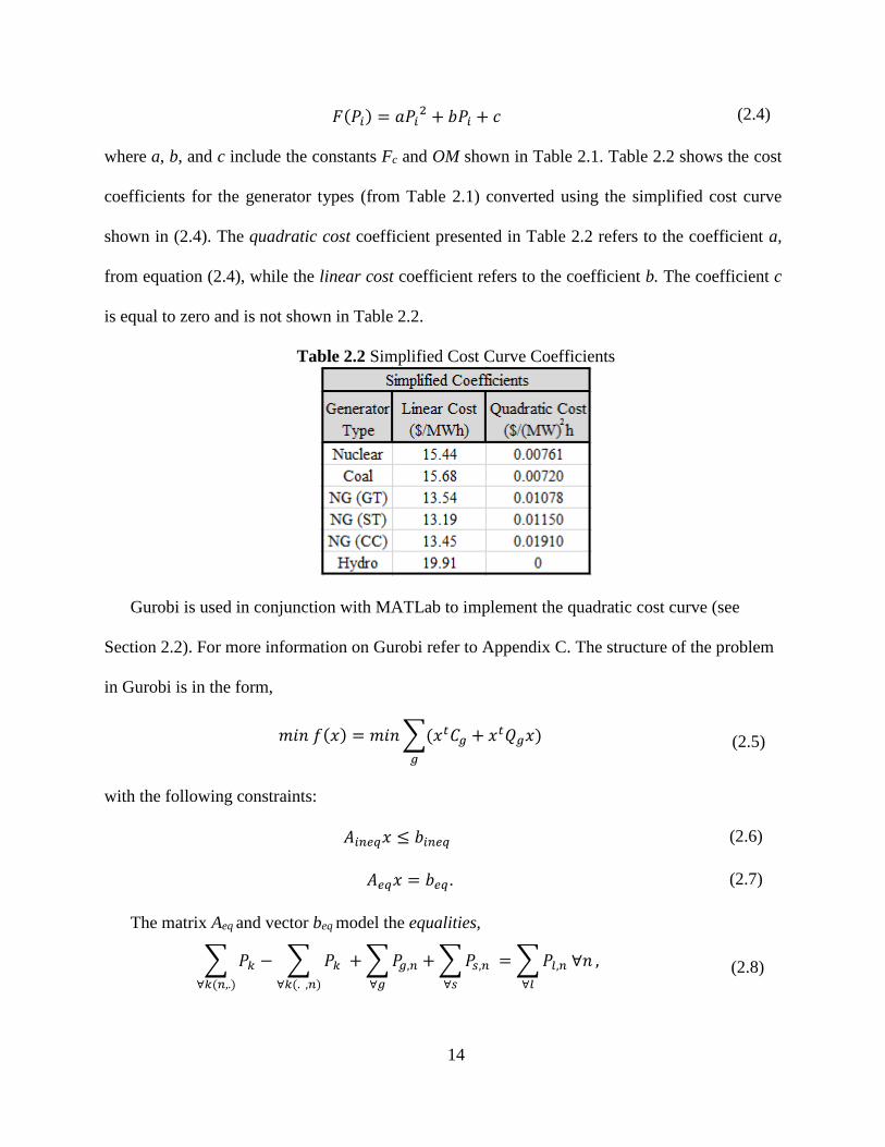
𝐹(𝑃𝑖) = 𝑎𝑃𝑖2 + 𝑏𝑃𝑖 + 𝑐 (2.4)
where a, b, and c include the constants Fc and OM shown in Table 2.1. Table 2.2 shows the cost
coefficients for the generator types (from Table 2.1) converted using the simplified cost curve
shown in (2.4). The quadratic cost coefficient presented in Table 2.2 refers to the coefficient a,
from equation (2.4), while the linear cost coefficient refers to the coefficient b. The coefficient c
is equal to zero and is not shown in Table 2.2.
Table 2.2 Simplified Cost Curve Coefficients
Gurobi is used in conjunction with MATLab to implement the quadratic cost curve (see
Section 2.2). For more information on Gurobi refer to Appendix C. The structure of the problem
in Gurobi is in the form,
𝑚𝑖𝑛 𝑓(𝑥) = 𝑚𝑖𝑛 ∑(𝑥𝑡𝐶𝑔 + 𝑥𝑡𝑄𝑔𝑥)
𝑔
(2.5)
with the following constraints:
𝐴𝑖𝑛𝑒𝑞𝑥 ≤ 𝑏𝑖𝑛𝑒𝑞 (2.6)
𝐴𝑒𝑞𝑥 = 𝑏𝑒𝑞. (2.7)
The matrix Aeq and vector beq model the equalities,
∑ 𝑃𝑘 − ∑ 𝑃𝑘 + ∑ 𝑃𝑔,𝑛 + ∑ 𝑃𝑠,𝑛 = ∑ 𝑃𝑙,𝑛 ∀𝑛
∀𝑙
,
∀𝑠∀𝑔∀𝑘(. ,𝑛)∀𝑘(𝑛,.)
(2.8)
Page 29
15
𝑃𝑘 − 𝐵𝑘(𝛿𝑛 − 𝛿𝑚) = 0 ∀𝑘, (2.9)
∑ 𝑃𝑠,𝑖 = 0 ∀𝑠.
∀𝑖
(2.10)
The matrix A and vector b model the inequalities,
−𝑃𝑘,𝑚𝑎𝑥 ≤ 𝑃𝑘 ≤ 𝑃𝑘,𝑚𝑎𝑥 ∀𝑘, (2.11)
𝑃𝑔,𝑚𝑖𝑛 ≤ 𝑃𝑔 ≤ 𝑃𝑔,𝑚𝑎𝑥; ∀𝑔, (2.12)
𝑃𝑠,𝑚𝑖𝑛 ≤ 𝑃𝑠 ≤ 𝑃𝑠,𝑚𝑎𝑥 ∀𝑠, (2.13)
0 ≤ 𝐸𝑠 ≤ 𝐸𝑠,𝑚𝑎𝑥 ∀𝑠, (2.14)
−𝑅𝑔 ≤𝑃𝑔,𝑖 − 𝑃𝑔,𝑖−1
∆𝑇≤ 𝑅𝑔 ∀𝑔; ∀𝑖 (2.15)
where the following notation is used:
Aeq Equality Constraint Matrix
Aineq Inequality Constraint Matrix
beq Equality Constraint Condition Vector
bineq Inequality Constraint Condition Vector
Bk Susceptance of Transmission Element k
Cg The Linear Coefficient, b, of the Cost Function of Generator g
Es The Energy Stored in Storage Unit s in MWh
Es,max Maximum Energy Capacity of Storage Unit s in MWh
f The Objective Function, Operating Cost
i Interval Number
k(.,n)
,n)
Set of Transmission Assets with n as the ‘FROM’ Node
k(n,.)
.)
Set of Transmission Assets with n as the ‘TO’ Node
m,n Bus Number (Nodes)
Page 30
16
Pg The Real Power Output of Generator g in MW
Pg,max Maximum Power Capacity of Generator g in MW
Pg,min Minimum Power Capacity of Generator g in MW
Pk The Power Flow of Transmission Line k in MW
Pk,max Maximum Line Flow Rating of Transmission Element k in MW
Pl The Active Power of Load l in MW
Ps The Real Power Output of Storage Unit s in MW
Ps,max Maximum Power Capacity of Storage Unit s in MW
Ps,min Minimum Power Capacity of Storage Unit s in MW
Qg The Quadratic Coefficient, a, of the Cost Function of Generator g
Rg Ramp Rate Limit of Generator g in 𝑀𝑊
ℎ𝑜𝑢𝑟
δk Bus Voltage Phase Angle at Node n or m
Δt Length of Interval i in Hours.
The vector x includes the bus voltage phase angles (δ), line flows (Pk), generator outputs (Pg), and
storage outputs (Ps) for each interval i. Note that most studies entail multiple time intervals (e.g.,
i = 1, 2, …, 24 for a one day study with each interval having a time span of Δt). Most of the
quantities listed above need to be specified for each individual time interval, and therefore the
notation indicated might also be written with an additional subscript, namely i. The equality
constraints in matrix Aeq and vector beq include the conservation of power at each bus (2.8), the
power flow across each line (2.9), and the charge/discharge of the storage elements (2.10). The
inequality constraints in matrix Aineq and vector bineq include the line flow limits (2.11), generator
Page 31
17
output limits (2.12), charging power storage limits (2.13), charging energy storage limits (2.14),
and the generator ramp rate limits (2.15).
Solving (2.8)-(2.15) gives the optimal x = x*, and also the optimal system wide operating
cost f(x) = f*.The operating cost then can be compared using two different models: one including
storage and another without storage to evaluate the effectiveness of storage in operating cost
reduction. The program is used with a model of the Arizona power grid to demonstrate the benefits
of adding pumped hydro energy storage to the system.
2.4 Problem formulation assumptions
In order to solve the economic dispatch problem, a set of assumptions were made in this thesis.
The following constraints (introduced in section 2.3) shown in Table 2.3 were observed in the
previous thesis by Ruggiero [1].
Table 2.3 Assumptions used in Ruggiero Thesis
Since the primary motivation of this thesis is to improve upon the accuracy of the referenced
thesis, a few of the assumptions were changed and included in the study. The key assumption
Page 32
18
changed was to include transmission line losses. The quadratic programming solver used in
Ruggiero’s thesis was Quadprog (a built-in MATLab function). Unfortunately, Quadprog has a
lot of limitations, the major one being that no quadratic constraints may be implemented into the
economic dispatch problem. Therefore, the mathematical solver Gurobi was substituted in for
Quadprog as it contained several more options that Quadprog did not provide. The main feature
of Gurobi that was of interest was the ability to implement quadratic constraints to the problem.
Refer to Appendix A for the code written in MATLab to utilize Gurobi as the mathematical
solver.
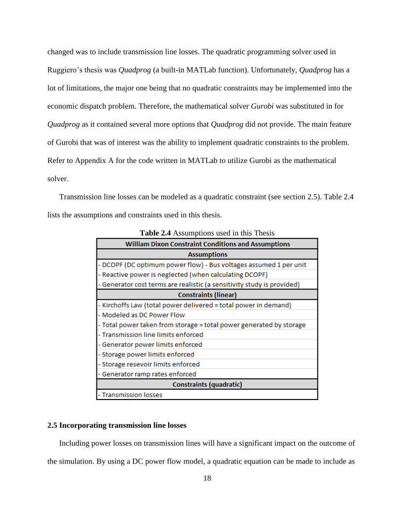
Transmission line losses can be modeled as a quadratic constraint (see section 2.5). Table 2.4
lists the assumptions and constraints used in this thesis.
Table 2.4 Assumptions used in this Thesis
2.5 Incorporating transmission line losses
Including power losses on transmission lines will have a significant impact on the outcome of
the simulation. By using a DC power flow model, a quadratic equation can be made to include as
Page 33
19
a quadratic constraint in the simulation. By creating this constraint, the simulation will take
transmission losses into account, making the final result more accurate. Please note: the following
derivation was originally going to be used to consider transmission losses into the system.
However, this method was found to not be compatible with Gurobi. The proceeding section
discusses the method eventually used to include transmission losses into the system. This
derivation is provided for purpose of future work in mind.
The quadratic programming method with Gurobi utilizing quadratic constraints is now used.
The objective function is still the same, restated below for convenience,
𝑀𝑖𝑛: 𝑥𝑡𝑄𝑥 + 𝑥𝑡𝐶 + 𝛼 (2.1)
where Q is the quadratic objective matrix (quadratic cost terms), C is the linear objective vector
(linear cost terms), and 𝛼 is a set constant (for the purpose of this thesis, 𝛼 = 0). The objective is
accompanied with a set of linear constraints,
𝐴𝑒𝑞𝑥 = 𝑏𝑒𝑞
𝐴𝑖𝑛𝑒𝑞𝑥 ≤ 𝑏𝑖𝑛𝑒𝑞
𝑙𝑜𝑤𝑒𝑟 𝑙𝑖𝑚𝑖𝑡 ≤ 𝑥 ≤ 𝑢𝑝𝑝𝑒𝑟 𝑙𝑖𝑚𝑖𝑡
(2.2)
and the constrained optimization is now augmented with a quadratic constraint,
𝑥𝑡𝐴𝑞𝑢𝑎𝑑𝑥 ≤ 𝑏𝑞𝑢𝑎𝑑 (2.16)
where the matrix Aquad contains the transmission line loss constraints. The contents to the Aquad
matrix is derived below.
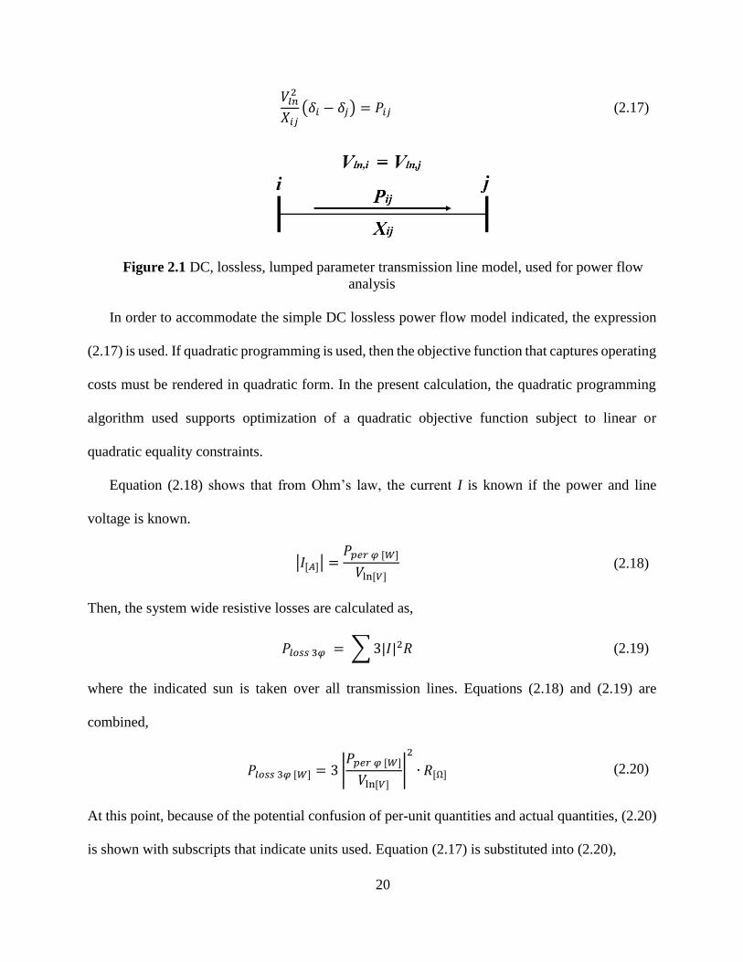
The basic DC power flow equation model [19, 20] is shown in equation (2.17). Figure 2.1
helps to illustrate (2.17). Note that this is a lossless, lumped parameter model of a transmission
line.
Page 34
20
𝑉𝑙𝑛2
𝑋𝑖𝑗(𝛿𝑖 − 𝛿𝑗) = 𝑃𝑖𝑗 (2.17)
Figure 2.1 DC, lossless, lumped parameter transmission line model, used for power flow
analysis
In order to accommodate the simple DC lossless power flow model indicated, the expression
(2.17) is used. If quadratic programming is used, then the objective function that captures operating
costs must be rendered in quadratic form. In the present calculation, the quadratic programming
algorithm used supports optimization of a quadratic objective function subject to linear or
quadratic equality constraints.
Equation (2.18) shows that from Ohm’s law, the current I is known if the power and line
voltage is known.
|𝐼[𝐴]| =𝑃𝑝𝑒𝑟 𝜑 [𝑊]
𝑉ln[𝑉] (2.18)
Then, the system wide resistive losses are calculated as,
𝑃𝑙𝑜𝑠𝑠 3𝜑 = ∑ 3|𝐼|2𝑅 (2.19)
where the indicated sun is taken over all transmission lines. Equations (2.18) and (2.19) are
combined,
𝑃𝑙𝑜𝑠𝑠 3𝜑 [𝑊] = 3 |𝑃𝑝𝑒𝑟 𝜑 [𝑊]
𝑉ln[𝑉]|
2
∙ 𝑅[Ω] (2.20)
At this point, because of the potential confusion of per-unit quantities and actual quantities, (2.20)
is shown with subscripts that indicate units used. Equation (2.17) is substituted into (2.20),
Page 35
21
𝑃𝑙𝑜𝑠𝑠 3𝜑 [𝑊] = 3𝑅[Ω] ∙1
𝑉ln [𝑉]2 ∙
(𝛿𝑖 − 𝛿𝑗)2
∙ 𝑉ln [𝑉]4
𝑋𝑖𝑗 [Ω]2 (2.21)
Equation (2.21) is then simplified, the units are changed to reflect megawatts (MW) instead of
watts (W), and the line-neutral voltage (Vln) is changed to line-line (Vll).
𝑃𝑙𝑜𝑠𝑠 3𝜑 [𝑀𝑊] = 3𝑅[Ω] ∙1
3∙ 𝑉ll [𝑉]
2(𝛿𝑖 − 𝛿𝑗)
2
𝑋𝑖𝑗 [Ω]2 ∙ 10−6 (2.22)
Finally, (2.22) is further simplified and the 10-6 term is removed by changing the units of the line-
line voltage from V to kV (the units are squared),
𝑃𝑙𝑜𝑠𝑠 3𝜑 [𝑀𝑊] = 𝑅[Ω] ∙ 𝑉ll[𝑘𝑉]2
(𝛿𝑖 − 𝛿𝑗)2
𝑋𝑖𝑗 [Ω]2 . (2.23)
The power loss equation is now in a quadratic form and may be used as a quadratic constraint in
the optimization software.
An alternative for the incorporation of transmission line losses
Due to a limitation in the Gurobi-MATLab interface, adding the quadratic constraints to the
program would cause an error because the Aquad matrix (containing the transmission line loss
quadratic constraints) was not a positive-semi-definite (PSD) matrix [21, 22]. The PSD attribute
of the Aquad matrix is required by Gurobi-MATLab for quadratic constraints, specifically because
Gurobi cannot solve non-convex constraints. PowerWorld Simulator (PW) was used as an
alternative solution to incorporate the losses. PW is a power system simulation package that
utilizes a robust Power Flow Solution engine capable of efficiently solving very large systems.
The PW user manual provides additional information on PW specifics [23].
In order to include the transmission losses in the economic dispatch problem, a combination
of the economic dispatch problem written in Gurobi-MATLab and PW is used. By forcing
generator power outputs to the pre-solved (no-loss) values, the total losses across the system are
Page 36
22
assumed to be picked up by the system slack bus. A list of assumptions for the PW configuration
are listed in Table 2.5.
Table 2.5 Assumptions made in PowerWorld
The following steps are taken to incorporate losses into the economic dispatch calculation:
1. A no-loss version of each case is solved for using the Gurobi-MATLab program
2. A PW case for each interval is created (containing the system topology [transmission
line and bus information])
3. The generator data (specifically the power output) for each time interval is taken from
step 1 and input into PW, the MW output for each generator is forced to not change
4. The generator per unit voltages are set to 1.15 for high load intervals and the reactive
power support for each generator is set to be in a realistic range (1 - 0.86 PF lagging)
5. The AC power flow is solved
6. Whatever the slack bus (at a Palo Verde bus) picks up is considered the total system
losses
7. Using a general participation factor for each load interval, the total system losses are
taken and dispatched as loads on each generator (and storage unit, if applicable for that
interval)
8. These “transmission loss loads” are added to the loads in each case, and the economic
dispatch is resolved using the Gurobi-MATLab program
Page 37
23
9. The result of the Gurobi-MATLab program now reflects transmission line losses
By following these steps, transmission losses can be incorporated iteratively into the economic
dispatch problem. This improves the accuracy of the results.
Page 38
24
CHAPTER 3: APPLICATION OF BULK ENERGY STORAGE IN ARIZONA
3.1 Description of the Arizona test bed
This chapter focuses on the presence of bulk energy storage (in the form of PHES) and
minimization of the total operating cost (subject to constraints) of the Arizona test bed. The effect
of energy storage on the minimization of the objective function (as stated in Section 2.3) is studied.
The Arizona electric grid is part of the Western Electricity Coordinating Council (WECC)
jurisdiction. Using the Arizona topology, generation limits, transmission limits, and the 2010
heavy summer load case, energy storage is added to appropriate buses in the system and operating
results are evaluated. The system data was provided by a state utility, Salt River Project (SRP).
The test bed used for this purpose is an equivalent system, including 115 kV and higher
transmission voltages.
The objective function (total operating cost in $/day) is minimized while the constraints and
formulation of the problem is the same as described in Chapter 2. Figure 3.1 illustrates the
principals of this concept.
Figure 3.1 Diagram of Concept of Adding PHES to Economic Dispatch Problem
Page 39
25
The quadratic programming algorithm explained in Section 2.3 is designed to optimize
generation while meeting the load demand at each interval and to schedule energy storage
appropriately (in the most economical way possible). The generation, line flow, and energy storage
(charging or discharging) schedule are control variables along with the bus voltage angles. These
values are calculated and the generation outputs are collaborated with the applicable generation
cost curves to determine the system wide operating costs.
The system load used is the Arizona 2010 summer peak, heavy load case. To approximate the
time variation of load in a day, the system wide load of 13,627 MW is multiplied by expression
(3.1) (this is the same method for approximating the load as was used by Ruggiero in the previous
thesis [1]),
0.45 cos (𝜋𝑡
12+ 0.5𝜋) + 0.55. (3.1)
Eight intervals of three hours each are used to replicate the common load profile during a 24
hour day, where t is the time at the beginning of each interval (e.g. t = 0, 3, 6,…, 21). This
approximate load profile is shown in Figure 3.2. The objective of the modeled system (depicted in
Figure 3.1) is to economically dispatch the available generation while optimally charging or
discharging the stored energy (utilizing peak shaving and/or load leveling as described in Section
1.3). The assumptions made for the described test bed are displayed in Table 3.1. The Arizona
system is an equivalenced system and this has the characteristics shown in Table 3.2.
Table 3.1 Test Bed Assumptions for this Thesis
Page 40
26
Figure 3.2 Arizona 2010 Summer Peak – Heavy Load Approximation using Piecewise
Linear Segments
Table 3.2 System Profile: an Equivalenced System used for this Thesis
The quadratic programming algorithm determines the total constrained optimum operating cost
of the system. The cost is then multiplied by 365 (days per year) to show the annual system wide
operating cost assuming the load modeled is the average over the entire year.
3.2 PHES facility locations
Since PHES was chosen as the form of energy storage for this thesis, preliminary research was
done to determine realistic locations for implementing PHES facilities in Arizona. There are two
types of locations that will be discussed: theoretical and currently planned.
Theoretical and hypothetical PHES locations
The theoretical (hypothetical, developed as examples assessed from the published literature)
locations were chosen for this thesis. Two of these locations are not currently being considered for
Page 41
27
PHES but the geographical properties (e.g. elevation differential, nearby water source, existing
reservoirs) of each location provide the opportunity to do so in the future. The facility sites were
chosen to be near existing hydroelectric dams in Arizona [24, 25].
There is a single pumped hydro facility in use in Arizona at the Horse Mesa Dam located in
Maricopa country [26]. The facility is operated by Salt River Project, and the level of energy
storage is low. The stated pumped storage power level is 130 MW. The engineering term used for
that facility is ‘pump back’ operation. Both Figure 3.3 and Table 3.5 in Section 3.3 give specific
information on the selected theoretical locations. Table 3.3 provides general information on each
project.
Table 3.3 Theoretical PHES Projects
Currently planned and potential future PHES locations
These locations were chosen since they are future projects currently awaiting approval from
FERC (Federal Energy Regulatory Commission) [27, 28]. Both indicated projects are in the
“Issued Preliminary Permits” stage. Both Figure 3.3 and Table 3.5 in Section 3.3 give specific
information on the future projects that were selected to model. Table 3.4 provides general
information on each project.
Page 42
28
Table 3.4 Future Planned PHES Projects
Longview Energy Exchange
This PHES project is currently in the “Issued Preliminary Permits” stage with FERC.
Located in Yavapai County, Arizona, the Longview project consists of constructing upper
reservoirs and a powerhouse. Around 650 acres of land would be used to host the upper
reservoir. Longview uses groundwater as the water source, thus a lower reservoir does not need
to be constructed. Underground tunnels will connect the ground water location to the upper
reservoir, these tunnels will not be visible above ground. The project reservoirs will be closed
loop, meaning that water in the reservoirs will be reusable [29]. The environmental concerns that
apply to the Longview project are briefly discussed below:
The source of water will be locally available ground water coming from the Big
Chino aquifer. This aquifer is used downstream by residents in Prescott, Prescott
Valley, and Chino Valley Arizona. There is general concern that the use of this water
by PHES will affect the water available for residents.
The Big Chino aquifer supplies 80% of the backflow of the Upper Verde River,
which is branded as one of the countries most endangered rivers because it is home to
many endangered species. There is concern that these species could be affected if the
PHES uses significant resources from that aquifer.
Page 43
29
Table Mountain Hydro
This PHES project is currently in the “Issued Preliminary Permits” stage with FERC.
Located in Mohave County, Arizona, the Table Mountain project consists of constructing a
concrete upper reservoir, lower reservoir, and powerhouse. The upper reservoir has the potential
to hold 5,280 acre-ft, with a water surface area of 66 acres. The lower reservoir has similar
values. The tunnel connecting both reservoirs is to be above ground. The proposed location will
be a closed loop orientation and the circulated reservoir will be reused [30]. An environmental
impact study has not yet been performed for this project.
3.3 Description of test cases
The Arizona transmission system described in Section 3.1 is tested using a few different cases.
The first case tested is without any energy storage added to the system. This case is analyzed to
determine a system wide operating cost that can be used to compare the operating cost of the cases
that include PHES.
The cases that include PHES look at locations in Arizona where PHES can be added (in some
circumstances, PHES is being already being considered at certain locations). Some of the chosen
locations to implement PHES are near existing hydroelectric dams in Arizona (e.g. Hoover
(Boulder) Dam, Glen Canyon Dam, and Horse Mesa Dam). PHES does not currently exist at these
locations and are used purely for simulation purposes. PHES is placed near existing dams because
of the high amount of water and elevation differential in the area. Figure 3.3 shows the locations
of the simulated PHES facilities on a map of Arizona.
Page 44
30
Specific information about these five PHES locations is provided in Table 3.5. These locations
were further discussed in Section 3.2. SRP designates the entity Salt River Project and WAPA
designates Western Area Power Administration.
Figure 3.3 Arizona Map with PHES Locations
Page 45
31
Table 3.5 Simulated PHES Location Specific Information
3.4 Arizona base case – summer 2010
The topology (described in Section 3.1) studied with no energy storage is considered the base
case (Case 0). The economic dispatch of the generators is determined by solving the quadratic
programming algorithm with the Gurobi-MATLab function. To reiterate, in order for the
constraints (listed in Section 3.1) to comply, reactive power is neglected (active power losses are
considered by the methods explained in Section 2.5). These constraints were previously shown in
Table 2.4, and is restated here for convenience.
The cost of ED of generation is calculated to be approximately $3.575 million per day, or
$1.305 billion per year. As expected, the total generation output matched the total system load
for each interval shown in Figure 3.2 (Section 3.1). The annual system operating cost from this
base case (Case 0) will be used for comparison with cases that include bulk energy storage.
Page 46
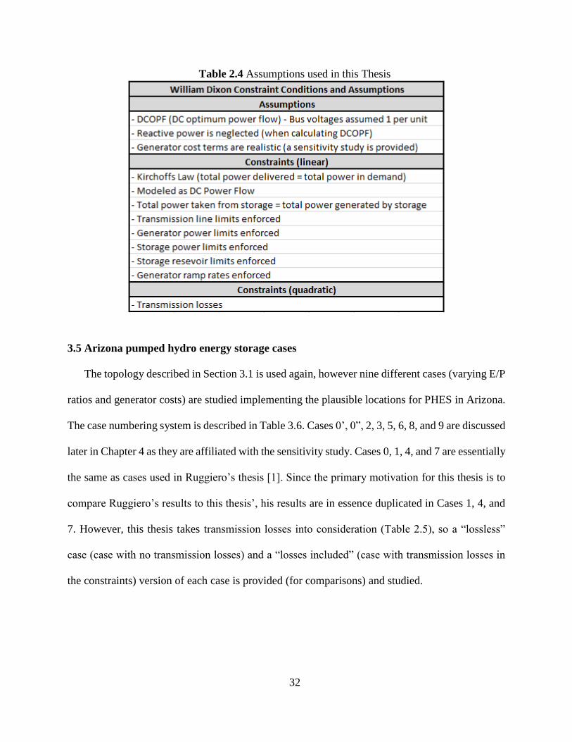
32
Table 2.4 Assumptions used in this Thesis
3.5 Arizona pumped hydro energy storage cases
The topology described in Section 3.1 is used again, however nine different cases (varying E/P
ratios and generator costs) are studied implementing the plausible locations for PHES in Arizona.
The case numbering system is described in Table 3.6. Cases 0’, 0”, 2, 3, 5, 6, 8, and 9 are discussed
later in Chapter 4 as they are affiliated with the sensitivity study. Cases 0, 1, 4, and 7 are essentially
the same as cases used in Ruggiero’s thesis [1]. Since the primary motivation for this thesis is to
compare Ruggiero’s results to this thesis’, his results are in essence duplicated in Cases 1, 4, and
7. However, this thesis takes transmission losses into consideration (Table 2.5), so a “lossless”
case (case with no transmission losses) and a “losses included” (case with transmission losses in
the constraints) version of each case is provided (for comparisons) and studied.
Page 47
33
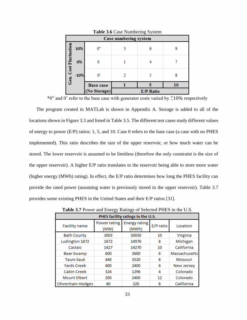
Table 3.6 Case Numbering System
*0” and 0’ refer to the base case with generator costs varied by 10%−
+ respectively
The program created in MATLab is shown in Appendix A. Storage is added to all of the
locations shown in Figure 3.3 and listed in Table 3.5. The different test cases study different values
of energy to power (E/P) ratios: 1, 5, and 10. Case 0 refers to the base case (a case with no PHES
implemented). This ratio describes the size of the upper reservoir, or how much water can be
stored. The lower reservoir is assumed to be limitless (therefore the only constraint is the size of
the upper reservoir). A higher E/P ratio translates to the reservoir being able to store more water
(higher energy (MWh) rating). In effect, the E/P ratio determines how long the PHES facility can
provide the rated power (assuming water is previously stored in the upper reservoir). Table 3.7
provides some existing PHES in the United States and their E/P ratios [31].
Table 3.7 Power and Energy Ratings of Selected PHES in the U.S.
Page 48
34
Table 3.8 shows the different cases studied in this thesis. Each E/P scenario shown is studied
for all storage facilities (active in the economic dispatch problem). These three cases are further
discussed in the sub-sections that follow.
Table 3.8 PHES Case Scenarios
3.5 Payback period calculation
The principal motivation of this thesis is to determine if PHES is an economically feasible
means of implementing energy storage into the Arizona electric grid. To determine this, the
payback period for building PHES systems into Arizona is of interest. The payback period will
give information regarding how long it would theoretically take to effectively “pay for” the PHES
facilities. The payback period compares the investment cost of the energy storage with the annual
savings. The time period calculated illustrates how long it would take to recover that initial
Page 49
35
investment. Since the economic dispatch problem will yield an annual operating cost number, the
annual savings (from adding bulk energy storage) can be calculated from the base case calculation
(Case 0, no energy storage, $1.305 per year). Using engineering economic principals equation
(3.2), the Uniform Series Present Worth equation, can be used to determine the payback period
given that the annual savings and initial investment is known [32].
(𝑃/𝐴, 𝑖%, 𝑛) =(1 + 𝑖)𝑛 − 1
𝑖(1 + 𝑖)𝑛 (3.2)
Equation (3.2) states that a present worth P (initial investment) can be calculated when the annual
payment A (annual operating cost savings), annual interest rate i, and number of compounding
periods n (years) is known. P, A, and i, are known, so n (the payback period), can be solved for.
For the purposes of this thesis, the annual interest rate, i, was assumed to be 0.25%.
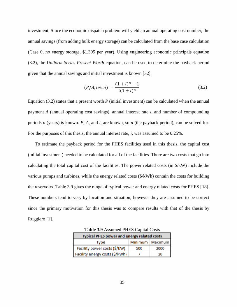
To estimate the payback period for the PHES facilities used in this thesis, the capital cost
(initial investment) needed to be calculated for all of the facilities. There are two costs that go into
calculating the total capital cost of the facilities. The power related costs (in $/kW) include the
various pumps and turbines, while the energy related costs ($/kWh) contain the costs for building
the reservoirs. Table 3.9 gives the range of typical power and energy related costs for PHES [18].
These numbers tend to very by location and situation, however they are assumed to be correct
since the primary motivation for this thesis was to compare results with that of the thesis by
Ruggiero [1].
Table 3.9 Assumed PHES Capital Costs
Page 50
36
Using the values from Tables 3.8 and 3.9, the capital cost of each PHES facility can be
calculated for each case. These values are shown in Table 3.10. Since a PHES facility already
exists at Horse Mesa Dam, the capital cost did not need to be calculated.
Table 3.10 PHES Facility Initial Investment Costs for Each Case
The total PHES capital cost for each case, annual savings for each case, along with equation
(3.2) is used to determine the payback period. The payback period for the three case scenarios is
later calculated in the proceeding sections after the annual operating savings is calculated for each
case.
Page 51
37
3.6 Summary of the results
In order to estimate the payback period and make progress towards determining the economic
value of PHES in Arizona, the annual operating costs of each case needed to be calculated. The
annual operating costs for each case was solved for by implementing the information presented in
the previous sections into Gurobi-MATLab (Appendix A).
Case 1 – E/P = 1, unaltered generator cost curves
In Case 1, the storage energy to power ratio (E/P) for each PHES facility was set to 1. Refer
back to Table 3.8 for specific information on how the E/P ratio effects the charging energy limit
for each PHES facility. The Case 1 data was input into the Gurobi-MATLab program, and the
steps outlined in Chapter 2 for implementing transmission losses into the problem were followed.
The annual operating cost without and with transmission losses was calculated to be $1.242 billion
and $1.305 billion respectively. Adding this PHES to the system resulted (when compared to the
base case, Case 0) in an annual savings of $63.0 million for both the lossless case and the case that
incorporated losses. The fact that the annual savings resulted in the same value for both cases is
simply a coincidence, as will be evident when the E/P ratio changes.
The results without incorporating losses are similar and in agreement with Ruggiero’s thesis
[1] findings. It is interesting to see that the annual operating cost of the system is increased by
4.02% (~$52 million) when incorporating losses into the problem. The importance of
incorporating transmission losses is reflected when the payback period is calculated from these
numbers (except for this case). The minimum payback period without and with transmission losses
was calculated to be 50 years for both cases. The maximum payback period was calculated to be
over 200 years.
Page 52
38
To really see the effect of adding PHES to the Arizona grid studied in this thesis, graphs were
created to illustrate the peak-shaving (or load-leveling) happening in the system. Refer back to
Section 1.3 for information on peak-shaving. Figure 3.4 shows the peak-shaving of Case 1 for the
lossless case (no transmission losses considered). Figure 3.5 shows the peak-shaving of Case 1 for
the case including losses (transmission losses considered).
Figure 3.4 Case 1 - Lossless Peak-Shaving
Figure 3.5 Case 1 – Losses Included Peak-Shaving
Page 53
39
It is difficult to visually inspect Figures 3.4 and 3.5 to determine the difference incorporating
losses has on peak shaving. Figure 3.4 (lossless case) can be seen to have slightly more energy
storage utilized for peak-shaving purposes. This is because it is more economical to do so as storing
more energy would increase the losses of the system. It is interesting to note that the system
automatically attempts to perform peak-shaving, without implementing any constraints in the
program that force it to do so. This proves that it is economically beneficial to perform peak-
shaving to a system.
Case 4 – E/P = 5, unaltered generator cost curves
In Case 4, the storage energy to power ratio (E/P) for each PHES facility was set to 5. Again,
the Case 4 data was input into the Gurobi-MATLab program. The annual operating cost without
and with transmission losses was calculated to be $1.192 billion and $1.264 billion respectively.
Adding this PHES to the system resulted (when compared to the base case, Case 0) in an annual
savings of $113.0 million and $93 million for the lossless case and the case that incorporated
losses, respectively. Now that the E/P ratio is not 1 (as it was in Case 1) it can be seen that the
annual savings for both the lossless case and losses included case is no longer the same value.
The results without incorporating losses are similar and in agreement with Ruggiero’s thesis
[1] findings. The annual operating cost of the system is increased by 5.70% (~$72 million) when
incorporating losses into the problem. Again, the importance of incorporating transmission losses
is reflected when the payback period is calculated from these numbers (except for this case). The
minimum payback period without and with transmission losses was calculated to be 29 years and
35 years respectively. The maximum payback period was calculated to be 128 years and 162 years
Page 54
40
respectively. Now it is apparent how much of an impact losses have on the system; the calculated
payback period ranges from 6 to 34 years longer when considering transmission losses.
Again, graphs were created to illustrate the peak-shaving (or load-leveling) happening in the
system. Figure 3.6 shows the peak-shaving of Case 4 for the lossless case (no transmission losses
considered). Figure 3.7 shows the peak-shaving of Case 4 for the case including losses
(transmission losses considered).
Figure 3.6 Case 4 – Lossless Peak-Shaving
Figure 3.7 Case 4 – Losses Included Peak-Shaving
Page 55
41
As was the same result from Case 1, Figure 3.6 (lossless case) can be seen to have slightly
more energy storage utilized for peak-shaving purposes than the case that incorporates losses
(Figure 3.7). It is interesting to note that Case 4 seems to perform more of a “load-leveling” method
than “peak-shaving” method (which was more apparent in Case 1). Again, this proves that it is
economically beneficial to perform peak-shaving (in this case, load-leveling) to a system.
Case 7 – E/P = 10, unaltered generator cost curves
In Case 7, the storage energy to power ratio (E/P) for each PHES facility was set to 10. Again,
the Case 7 data was input into the Gurobi-MATLab program. The annual operating cost without
and with transmission losses was calculated to be $1.185 billion and $1.266 billion respectively.
Note that the annual operating cost in the case that includes transmission losses has increased, not
decreased, when changing the E/P from 5 to 10. This is due to the program attempting to minimize
the cost due to losses. What can be concluded from this, is that a greater E/P ratio does not
necessarily correlate to a cheaper annual operating cost. But this was only determined by
considering transmission losses.
Adding this PHES to the system resulted (when compared to the base case, Case 0) in an
annual savings of $130.0 million and $91 million for the lossless case and the case that
incorporated losses, respectively (again note the difference of Case 4 and Case 7).
The results without incorporating losses are similar and in agreement with Ruggiero’s thesis
[1] findings. The annual operating cost of the system is increased by 6.40% (~$81 million) when
incorporating losses into the problem. Again, the importance of incorporating transmission losses
is reflected when the payback period is calculated from these numbers (except for this case). The
minimum payback period without and with transmission losses was calculated to be 29 years and
38 years respectively. The maximum payback period was calculated to be 126 years and 176 years
Page 56
42
respectively. Now it is apparent how much of an impact losses have on the system; the calculated
payback period ranges from 9 to 50 years longer when considering transmission losses.
Figure 3.8 shows the peak-shaving of Case 7 for the lossless case (no transmission losses
considered). Figure 3.9 shows the peak-shaving of Case 7 for the case including losses
(transmission losses considered).
Figure 3.8 Case 7 – Lossless Peak-Shaving
Figure 3.9 Case 7 – Losses Included Peak-Shaving
As was the same result from Case 1 and 4, Figure 3.4 and 3.6 (lossless cases) respectively can
be seen to have slightly more energy storage utilized for peak-shaving purposes. It is interesting
to note that Case 7 seems to overshoot a load-leveling condition, this is due to more storage being
Page 57
43
available (E/P = 10) than was in Case 4 (E/P = 5). Once again, this proves that it is economically
beneficial to perform peak-shaving (in this case, load-leveling) to a system.
3.7 Conclusions
In Section 3.6, the effects of implementing PHES was studied in 3 different cases (Cases 1, 4,
7). The lossless (transmission losses not considered) essentially reflect Ruggiero’s findings [1].
This thesis took the previous thesis one step further and implemented transmission losses into the
constraints. The results from Section 3.6 showed that incorporating transmission losses into the
calculations is important, as it had a large influence on the annual operating cost, and ultimately,
the payback period.
While these results are noteworthy and will assist in justifying the use of PHES in the Arizona
power grid, there are a lot of assumptions. One of the primary assumptions of Ruggiero’s thesis,
is that the generator cost curves for each unit type are realistic numbers. While this may be true, it
is impossible to know for certain since the cost curves are confidential and not given out by the
entities governing the generators. Chapter 4 provides a sensitivity study of the generator costs.
Page 58
44
CHAPTER 4: SENSITIVITY STUDY OF GENERATION COSTS
4.1 Deviation of generator cost curves
One of the primary goals of this thesis was to eliminate the amount of assumptions used.
Assumptions may yield results, but a slight tweak in the data (in this case, the generator cost
curves) may produce a completely different answer. In order to get a better understanding of the
possible effects of the generator cost curve numbers being incorrect, a sensitivity study has been
provided to determine how much the generator cost curves impact the economic dispatch problem.
In Section 2.3, Table 2.2 (restated here for convenience) provided the simplified (put into
quadratic form) cost curve coefficients for each generator type. The following nomenclature is
used in Table 2.2.
NG – Natural gas
GT – Gas turbine
ST – Steam turbine
CT – Combined cycle plant
Table 2.2 Simplified Cost Curve Coefficients
A sensitivity study is used to recalculate the data and the results for Cases 0, 1, 4, and 7. Both
the linear and quadratic cost coefficients were varied by 10%−+ . Tables 4.1 and 4.2 show the
Page 59
45
resultant cost curve coefficients for each type of generator. These new generator cost coefficients
(or cost curves) are used in this sensitivity study.
Table 4.1 Simplified Cost Curve Coefficients Varied by +10%
Table 4.2 Simplified Cost Curve Coefficients Varied by -10%
4.2 Description of sensitivity study cases
The topology described in Section 3.1 is used again. However, nine different cases (varying
E/P ratios and generator costs) are studied implementing the plausible locations for PHES in
Arizona. The case numbering system is described in Section 3.4 in Table 3.4, it is restated below
for convenience. Cases 2, 3, 5, 6, 8, and 9 are discussed here in the sensitivity study. Cases 1, 4,
and 7 are essentially the same as cases used in Ruggiero’s thesis [1] (the lossless cases), and were
discussed in Chapter 3. Since the primary motivation of this thesis is to compare Ruggiero’s
results, they are duplicated in Cases 1, 4, and 7. However, it is desirable to account for transmission
losses (Table 2.5). Therefore a “lossless” (case with no transmission losses) and a “losses
Page 60
46
included” (case with transmission losses in the constraints) version of each case is provided (for
comparisons) and studied. Refer back to Chapter 3 for specifics on the locations of the PHES
facilities (Section 3.3) and the methods used to solve each test case (Section 3.6).
Table 3.4 Case Numbering System
*0” and 0’ refer to the base case with generator costs varied by 10%−
+ respectively
4.3 Sensitivity study results
In order to determine the outcome of the sensitivity study and estimate the payback period, the
annual operating costs of each case needed to be calculated. The annual operating costs for each
case was solved for by implementing the information presented in the previous sections into
Gurobi-MATLab (Appendix A). Section 3.6 discussed specifics into the results of each case, a lot
of the comments made can be extrapolated and applied here. The graphs that describe the peak-
shaving for each case have been provided in Appendix B for desired reference, as they are very
similar to those that were presented in Section 3.6.
In each case, the storage energy to power ratio (E/P) for each PHES facility was varied
depending on the case; for cases 1-3: E/P = 1, for cases 4-6: E/P = 5, for cases 7-9: E/P = 10. The
case specific data were input into the Gurobi-MATLab program, and the steps outlined in Section
2.5 for implementing transmission losses into the problem were followed. The annual operating
cost without and with transmission losses was calculated for each case, shown in Tables 4.3 and
Page 61
47
4.4 in a convenient manor such that each cases numbers can be compared easily (including the
results from Cases 1, 4, and 7). Adding PHES to the system results in an annual savings when
compared to the base cases, namely Cases 0, 0’, and 0”. The annual savings for each case appear
in Tables 4.5 and 4.6.
Table 4.3 Calculated System Annual Operating Costs (no Transmission Losses)
Table 4.4 Calculated System Annual Operating Costs (with Transmission Losses)
Table 4.5 Calculated System Annual Savings from Adding PHES (no Transmission Losses)
Page 62
48
Table 4.6 Calculated System Annual Savings from Adding PHES (with Transmission Losses)
The annual savings can be used to calculate the payback period. Tables 4.7-4.10 provide the
calculated minimum and maximum payback period for each case studied.
Table 4.7 Minimum Payback Period (no Transmission Losses)
Table 4.8 Minimum Payback Period (with Transmission Losses)
Page 63
49
Table 4.9 Maximum Payback Period (no Transmission Losses)
Table 4.10 Maximum Payback Period (with Transmission Losses)
Page 64
50
CHAPTER 5: CONCLUSIONS AND FUTURE WORK
5.1 Conclusions
In this thesis, a test bed utilizing the Arizona transmission system (with a 2010 summer peak
load) was used to demonstrate several topics related to bulk energy storage. The following
conclusions can be made based on the research and results obtained:
The economic dispatch problem
Chapter 2 contains a discussion of the economic dispatch problem and provided the
methodology used to solve the problem. Quadratic programming is chosen as the method to solve
the economic dispatch problem and simulate energy storage and its effect on the Arizona power
grid.
Addition of energy storage
Chapter 3 shows the calculation of the minimum annual operating cost of the system with no
energy storage. Chapters 3 and 4 both discussed the outcome of implementing large levels of PHES
in the Arizona power grid. Tables 4.3 and 4.4 (in Section 4.3) state the annual operating costs for
all cases. Since adding transmission losses to the problem was a primary motivation of this thesis,
Table 5.1 gives a comparison (percent increase) of the “lossless” and “losses included” annual
operating costs for each case.
Table 5.1 Annual Operating Cost Percent Increase
Page 65
51
It makes sense that the difference between the “lossless” and “losses included” annual
operating costs increased with an increase of the E/P ratio. With an increase in the E/P ratio, the
amount of storage being utilized will increase, therefore the losses will increase. In Section 4.3,
Tables 4.7-4.10 showed the calculated payback periods for each case. Table 5.2 and 5.3 present
the percent increase of the “lossless” and “losses included” payback periods. This percent
difference data shows that including transmission losses in the problem formulation and
calculation is important. The payback period increased by ~28% in some cases.
Table 5.2 Best Case (Cheapest Storage Costs) Payback Period Percent Increase
Table 5.3 Worst Case (Most Expensive Storage Costs) Payback Period Percent Increase
This percent difference data shows that including transmission losses in the problem formulation
and calculation is important. The payback period increased by ~28% in some cases.
Page 66
52
Sensitivity study – generator cost deviation
One of the primary goals of this thesis was to alleviate the assumptions used. For example, a
small variation in generation cost data may result in different conclusions. In order to obtain a
better understanding of the effects of the generator cost inaccuracy, a sensitivity study was
provided in Chapter 4 to assess the impact on the economic dispatch problem.
After examining the results as indicated in Section 4.3, the percent increase from perturbing
the generator cost was calculated. Table 5.4 and 5.5 present the percent increase of the annual
operating cost from adjusting the generator costs. This percent increase data shows that fluctuating
the generator costs did exactly what was expected. When increasing all of the generator costs by
10% (Cases 3, 6, and 9), the annual operating costs increase by approximately 10% and vice-versa
for Cases 2, 5, and 8. The percent increase of the payback period due to changing the generator
costs was also calculated and is displayed in Tables 5.6-5.9.
Table 5.4 Percent Increase of Annual Operating Cost from Deviating the Generator Costs
Table 5.5 Percent Increase of Annual Operating Cost from Deviating the Generator Costs
Page 67
53
Table 5.6 Best Case Payback Period Percent Increase from Deviating the Generator Cost
Table 5.7 Best Case Payback Period Percent Increase from Deviating the Generator Cost
Table 5.8 Worst Case Payback Period Percent Increase from Deviating the Generator Cost
Table 5.9 Worst Case Payback Period Percent Increase from Deviating the Generator Cost
Note that the payback period actually decreases when the generator costs increase. This is due
to the annual savings of implementing PHES increases proportional to the generator cost increase.
Observe that (for the worst case) the percent increase in the operating cost is zero with an E/P ratio
Page 68
54
of 1. This is due to the payback period being out of range of the calculation (listed as 200+, or
unfeasible).
Final comments
The research supports the conclusion that the most feasible PHES scenario would be to have
an E/P ratio of about 5, as the payback period is the lowest (when including transmission losses).
The sensitivity study showed that if the assumed generator costs were inaccurate, the payback
period for each case will adjust proportional to the adjustment of the generator costs. For example,
if the assumed generation costs are too low (the actual generation costs are 10% higher) then the
resulting payback period would be approximately 10% lower than what was originally calculated.
5.2 Future work
In the research and tests performed for this thesis, the economic dispatch was studied using the
Arizona test bed with various simplifying assumptions. This thesis in particular, attempted to
remove some of the assumptions made by Ruggiero’s thesis [1]. However, some assumptions were
carried on from the previous thesis, particularly: modeling reactive power flows, energy storage
losses, system voltages and their limits. The present engineering study could be enhanced in the
following ways:
One important point not fully discussed in the present thesis is the impact of efficiency
in the pumped hydro cycle. The efficiency of the cycle for modern units is estimated
at higher than 90%. Inclusion of pumped hydro losses is relegated to future work.
Performing an ACOPF (unlike the one mentioned in Section 2.5) on the Arizona test
bed to model and incorporate bus voltage and transient system stability in an N-1
analysis
Page 69
55
Model reactive power in the system analysis and quantify its effects
Modeling the correct bus voltages in the system
Extending the analysis out to the entire WECC interconnection and determining PHES
locations in the larger system
Incorporation of examples of lowering the transmission line congestion in the system
with implementation of energy storage.
In this thesis, the full capabilities of Gurobi are not utilized (e.g., integer variables, binary
variables). However, the formulation shown here does create a platform such that future, more
sophisticated modeling may readily be incorporated.
Page 70
56
REFERENCES
[1] J. Ruggiero, “The cost and benefit of bulk energy storage in the Arizona power
transmission system,” M.S. thesis, Arizona State University, Tempe AZ, December 2013.
[2] B. Kang, H. Yoon, Su. Park, B. Lee, Se. Park, “Design and implementation of intelligent
energy storage service model for peak load shaving,” IEEE International Conference on
Consumer Electronics, 10-13 January 2014, Las Vegas, NV, pp. 548-549.
[3] R.J. Kerestes, G.F. Reed, A.R. Sparacino, "Economic analysis of grid level energy storage
for the application of load leveling," IEEE Power and Energy Society General Meeting,
22-26 July 2012, pp. 1-9.
[4] Z. Hu, F. Zhang, B. Li, “Transmission expansion planning considering the deployment of
energy storage systems,” IEEE Power and Energy Society General Meeting, 22-26 July
2012, pp. 1-6.
[5] D. Mears, H. Gotschall, T. Key, H. Kamath, “EPRI-DOE handbook of energy storage for
transmission and distribution applications,” EPRI, Palo Alto, CA, 2003.
[6] Arizona Corporation Commission, “Renewable energy standard & tariff,” available at:
http://www.azcc.gov/divisions/utilities/electric/environmental.asp
[7] P. Denholm, E. Ela, B. Kirby, M. Milligan, “The role of energy storage with renewable
electricity generation,” NREL, 2010, available at:
http://www.nrel.gov/docs/fy10osti/47187.pdf.
[8] K. Qian, Z. Li, C. Zhou, Y. Yuan, “Benefits of energy storage in power systems with high
level of intermittent generation,” IEEE 20th International Conference and Exhibition on
Electricity Distribution, 8-11 June 2009, pp. 1-4.
[9] D. Li-jie, W. Biao, Z. Hua, R. Zeng, Q. Xiao-yan, “The optimal allocation of pumped
storage station in wind farm,” IEEE Power and Energy Engineering Conference Asia-
Pacific, 27-29 March 2012, pp. 1-4.
[10] Bonneville Power Administration, “BPA balancing authority load and total wind, hydro,
and thermal generation, near-real-time,” available at:
http://transmission.bpa.gov/Business/Operations/Wind/baltwg.aspx
[11] DOE Global Energy Storage Database, “Castaic pumped-storage plant,” available at:
http://www.energystorageexchange.org/projects/185.
[12] W.F. Pickard, “The history, present state, and future prospects of underground pumped
hydro for massive energy storage,” Proceedings of the IEEE, February 2012, vol. 100, no.
2, pp. 473-483.
Page 71
57
[13] F. Barnes; J. Levine, Large energy storage systems handbook, CRC Press – Taylor &
Francis Group, Boca Raton, FL, 2011.
[14] J. Zhu, Optimization of power system operation, J Wiley and Sons, Piscataway, NJ, First
edition, 2009.
[15] W. Ongsakul, V. N. Dieu, Artificial intelligence in power system optimization, CRC Press,
Boca Raton, FL, 2013.
[16] N. M. Pindoriya, S.N. Singh, K.Y. Lee, "A comprehensive survey on multi-objective
evolutionary optimization in power system applications," IEEE Power and Energy Society
General Meeting, 25-29 July 2010, pp. 1-8.
[17] H. H. Happ, “Optimal power dispatch-a comprehensive survey,” IEEE Transactions on
Power Apparatus and Systems, May-June 1977, vol. 96, pp. 841-854.
[18] S. Eftekharnejad, “The Impact of increased penetration of photovoltaic generation on
smart grids,” PhD. dissertation, Arizona State University, Tempe AZ, December 2012, pp.
48.
[19] F. Li, R. Bo, “DCOPF-based LMP simulation: algorithm, comparison with ACOPF, and
sensitivity,” IEEE Transactions on Power Systems, November 2007, vol. 22, no. 4, pp.
1475-1485.
[20] B. Wollenberg, A. Wood, Power generation operation and control, J Wiley and Sons,
New York, Second edition, 1996, pp. 108.
[21] UC San Diego, Department of Mathematics, “Positive semidefinite matrices,” available
at:
http://www.math.ucsd.edu/~njw/Teaching/Math271C/Lecture_03.pdf
[22] Gurobi Optimization, “Gurobi MATLab reference manual,” available at:
http://www.gurobi.com/documentation/5.6/reference-manual/matlab_reference_manual
[23] PowerWorld, “PowerWorld Simulator 18 manual,” available at:
http://www.powerworld.com/WebHelp/.
[24] U.S. Department of the Interior – Bureau of Reclamation, “Upper Colorado region,”
available at:
http://www.usbr.gov/uc/rm/crsp/gc/index.html
[25] U.S. Department of the Interior – Bureau of Reclamation, “Hoover Dam facts and
figures,” available at:
http://www.usbr.gov/lc/region/pao/brochures/faq.html
Page 72
58
[26] Salt River Project, “Horse Mesa Dam,” available at:
http://www.srpnet.com/water/dams/horsemesa.aspx
[27] Federal Energy Regulatory Commission, “Hydropower Licensing: Preliminary Permits,”
Washington DC, available at:
http://www.ferc.gov/industries/hydropower/gen-info/licensing/pre-permits.asp
[28] Federal Energy Regulatory Commission, “Issued Preliminary Permits for Pumped
Storage Projects Map,” Washington DC, available at:
http://www.ferc.gov/industries/hydropower/gen-info/licensing/pump-storage/issued-
permits.pdf
[29] K. F. Kumli, “Application for preliminary permit for the Longview Pumped Storage
project,” available at:
http://longviewee.com/admins/wp-content/uploads/2012/02
/Application%20for%20Preliminary%20Permit.pdf.
[30] Table Mountain LLC, “Table Mountain Pumped Storage project: notice of preliminary
permit,” available at:
http://www.gpo.gov/fdsys/pkg/FR-2011-11-14/pdf/2011-29248.pdf.
[31] U. S. Department of Energy, “DOE international energy storage database: open loop
pumped hydro storage,” Washington DC, available at:
http://www.energystorageexchange.org/projects?utf8=%E2%9C%93&technology_type_s
ort_eq=Open+Loop++Pumped+Hydro+Storage&country_sort_eq=&state_sort_eq=&kW
=&kWh=&benefit_stream_inf=&ownership_model_eq=&status_eq=&siting_eq=&show
_unapproved=%7B%7D&order_by=&sort_order=&search_page=1&size_kw_ll=&size_
kw_ul=&size_kwh_ll=&size_kwh_ul=.
[32] Georgia Institute of Technology, “Engineering Economics,” Atlanta, GA, available at:
http://www-old.me.gatech.edu/jonathan.colton/me4210/fe_engineering_economics.pdf
[33] Gurobi Optimizer, “Solving models with the Gurobi MATLAB interface,” available at:
http://www.gurobi.com/documentation/5.6/reference-
manual/matlab_solving_models_with
[34] Gurobi Optimizer, “gurobi() reference manual,” available at:
http://www.gurobi.com/documentation/5.6/reference-manual/matlab_gurobi
Page 73
59
APPENDIX A
MATLAB CODE
Page 74
60
A.1 MATLab code: formulate and solve the economic dispatch for the annual cost
% ARIZONA STATE UNIVERSITY % M.S. Thesis Work % Student: William J. J. Dixon % Advisor: Gerald T. Heydt % Date: Fall 2014 % Purpose: This code puts real data (buses, lines, gens, etc.) into an % appropriate matrix form min: x^t*Q*x + C*x in order to calculate % a DCOPF. Numerous constraints are included (line limits, gen ramp % rates, etc.)
clear
%% Import data filename = 'Case0_losses_data.xlsx';
%Reads xlsx file with real network data A=xlsread(filename,'System data'); %Determines number of each category b=A(1,1); % b=# of buses l=A(1,2); % l=# of lines g=A(1,3); % g=# of generators s=A(1,4); % s=# of storage units int=A(1,5); % int=# of load intervals dT=A(1,6); % dT= delta t or hours per
interval d=A(1,7); % d=number of days B=xlsread(filename,'Bus data'); %Extracts bus data L=xlsread(filename,'Line data'); %Extracts line data G=xlsread(filename,'Generator data'); %Extracts generator data S=xlsread(filename,'Storage data'); %Extracts storage data
X=(3*b+l-1)*int; %Creates size of 'x' matrix
%% Generate Matrices
%% GENERATION OF THE Q MATRIX (QUADRATIC COSTS)
%Extracts generator quadratic cost terms and inputs into a matrix c=1; j=1; a=zeros(b,b); for k=1:1:g
a(G(c,1),G(c,1))=G(c,5)*2; c=c+1; j=j+1; end %Matrix of generator quadratic costs at each hour c=1; j=1; for k=1:1:int
Page 75
61
Q1(c:c+b-1,j:j+b-1)=a; c=c+b; j=j+b; end %Overall Q matrix with Q1 in the correct location Q=zeros(X,X); Q((b+l-1)*int+1:(2*b+l-1)*int,(b+l-1)*int+1:(2*b+l-1)*int)=Q1; Q=sparse(Q);
%% GENERATION OF THE C MATRIX (LINEAR COSTS)
%Extracts generator linear cost terms and inputs them into a matrix c=1; j=1; C1=zeros(1,b); for k=1:1:g
C1(1,G(c,1))=G(c,4); c=c+1; j=j+1; end %Repeats the linear costs over the amount of hours j=1; for k=1:1:int
CT(1,j:j+b-1)=C1; j=j+b; end %Inputs the total linear costs into the overall C matrix C=zeros(1,X); C(1,(b+l-1)*int+1:(2*b+l-1)*int)=CT; C=sparse(C);
%% GENERATION OF THE B MATRIX (INEQUALITY LIMITS)
%Generates vector of line limits c=1; j=1; b1=zeros(2*l*int,1); for k=1:1:l
b1(c:2*j*int,1)=L(j,6); c=c+2*int; j=j+1; end %Generates vector of generator limits i=1; j=1; b2=zeros(2*b*int,1); b2i=zeros(2*int,1); for k=1:1:g for u=1:1:int b2i(i,1)=G(j,3); b2i(i+1,1)=-G(j,2); i=i+2;
Page 76
62
end b2(2*G(j,1)*int-(2*int-1):2*G(j,1)*int,1)=b2i; j=j+1; i=1; b2i=zeros(2*int,1); end %Generates vector of storage charging power limits i=1; j=1; b3=zeros(2*b*int,1); b3i=zeros(2*int,1); for k=1:1:s for u=1:1:int b3i(i:i+1,1)=S(j,2); i=i+2; end b3(2*S(j,1)*int-(2*int-1):2*S(j,1)*int,1)=b3i; j=j+1; i=1; b3i=zeros(2*int,1); end %Generates vector of generator ramp rate limits i=1; j=1; b4=ones(2*b*(int-1),1)*10000; b4i=zeros(2*(int-1),1); for k=1:1:g for u=1:1:(int-1) b4i(i:i+1,1)=G(j,6); i=i+2; end b4(2*G(j,1)*(int-1)-(2*(int-1)-1):2*G(j,1)*(int-1),1)=b4i; j=j+1; i=1; b4i=zeros(2*(int-1),1); end %Generates vector of storage charging energy limits i=1; j=1; b5=zeros(2*b*int,1); b5i=zeros(2*int,1); for k=1:1:s for u=1:1:int b5i(i,1)=S(j,3); b5i(i+1,1)=0; i=i+2; end b5(2*S(j,1)*int-(2*int-1):2*S(j,1)*int,1)=b5i; j=j+1; i=1; b5i=zeros(2*int,1); end %Inputs 5 vectors (b1,b2,b3,b4 and b5) into overall b vector bT=zeros(2*int*(l+2*b)+2*b*(int-1)+2*b*int,1); bT(1:2*l*int,1)=b1; bT(2*l*int+1:2*int*(l+b),1)=b2; bT(2*int*(l+b)+1:2*int*(l+2*b),1)=b3;
Page 77
63
bT(2*int*(l+2*b)+1:2*int*(l+2*b)+2*b*(int-1),1)=b4; bT(2*int*(l+2*b)+2*b*(int-1)+1:2*int*(l+2*b)+2*b*(int-1)+2*b*int,1)=b5; bT=sparse(bT);
%% GENERATION OF THE beq MATRIX (EQUALITY LIMITS)
%Generates beq1 vector which contains the load value at each bus and each %interval c=1; j=1; m=1; beqa=zeros(int,1); beq1=zeros(b*int,1); for k=1:1:b p=5; for u=1:1:int beqa(c,1)=B(j,p); c=c+1; p=p+1; end c=1; beq1(m:int*j,1)=beqa; m=m+int; j=j+1; end %Inputs load values into the overall beq vector with zeros at every other %point beq=zeros((b+l)*int+b,1); beq(l*int+1:(l+b)*int,1)=beq1; beq=sparse(beq);
%% GENERATION OF THE A MATRIX (INEQUALITY CONSTRAINTS)
%Generates the A1 matrix(line inequalities) t=1; i=1; j=1; m=1; A1=zeros(2*l*int,l*int); %Sets up size of A1 matrix A1i=zeros(2*int,l*int); %Sets up size of inner A1i matrix for k=1:1:l for u=1:1:int A1i(i,j)=1; A1i(i+1,j)=-1; i=i+2; j=j+l; end A1(m:2*t*int,1:l*int)=A1i; %Inputs inner matrix of each m=m+2*int; %line into the larger A1 matrix t=t+1; i=1; j=t; A1i=zeros(2*int,l*int); end; %Generates the A2 matrix(generator inequalities) t=1;
Page 78
64
i=1; j=1; m=1; A2=zeros(2*b*int,b*int); %Sets up size of A2 matrix A2i=zeros(2*int,b*int); %Sets up size of inner A2i matrix for k=1:1:b for u=1:1:int A2i(i,j)=1; A2i(i+1,j)=-1; i=i+2; j=j+b; end A2(m:2*t*int,1:b*int)=A2i; m=m+2*int; t=t+1; i=1; j=t; A2i=zeros(2*int,b*int); end %Generates A3 matrix (storage inequalities) t=1; i=1; j=1; m=1; A3=zeros(2*b*int,b*int); %Sets up size of A3 matrix A3i=zeros(2*int,b*int); %Sets up size of inner A3i matrix for k=1:1:b for u=1:1:int A3i(i,j)=1; A3i(i+1,j)=-1; i=i+2; j=j+b; end A3(m:2*t*int,1:b*int)=A3i; %Inputs inner matrix of each m=m+2*int; %storage into the larger A3
matrix t=t+1; i=1; j=t; A3i=zeros(2*int,b*int); end; %Generates the A4 matrix(generator ramp rate inequalities) i=1; j=1; m=1; t=1; A4=zeros(2*b*(int-1),b*int); A4i=zeros(2*(int-1),b*int); for k=1:1:b for u=1:1:(int-1) A4i(i,j)=1/dT; A4i(i,j+b)=-1/dT; A4i(i+1,j)=-1/dT; A4i(i+1,j+b)=1/dT; i=i+2; j=j+b; end
Page 79
65
A4(m:2*t*(int-1),1:b*int)=A4i; m=m+2*(int-1); t=t+1; i=1; j=t; A4i=zeros(2*(int-1),b*int); end %Generates the A5 matrix (bulk energy storage limit on energy storage) i=1; j=1; t=0; z=1; f=1; y=int; A5=zeros(2*b*int,b*int); A5i=zeros(2*int,b*int); for k=1:1:b for m=1:1:int for u=1:1:y A5i(i+2*t,j)=dT; A5i(i+2*t+1,j)=-dT; i=i+2; end i=1; y=y-1; t=t+1; j=j+b; end A5(f:2*z*int,1:b*int)=A5i; y=int; f=f+2*int; z=z+1; j=z; t=0; A5i=zeros(2*int,b*int); end %Stores each of the smaller matrices (A1,A2,A3,A4, and A5) into the A matrix A=zeros(2*int*(l+2*b)+2*b*(int-1)+2*b*int,X); A(1:2*l*int,(b-1)*int+1:(b+l-1)*int)=A1; A(2*l*int+1:2*int*(l+b),(b+l-1)*int+1:(2*b+l-1)*int)=A2; A(2*int*(l+b)+1:2*int*(l+2*b),(2*b+l-1)*int+1:X)=A3; A(2*int*(l+2*b)+1:2*int*(l+2*b)+2*b*(int-1),(b+l-1)*int+1:(2*b+l-1)*int)=A4; A(2*int*(l+2*b)+2*b*(int-1)+1:2*int*(l+2*b)+2*b*(int-1)+2*b*int,(2*b+l-
1)*int+1:X)=A5; %A=sparse(A);
%% GENERATION OF THE AEQ MATRIX (EQUALITY CONSTRAINTS)
Aeq=zeros((b+l)*int+s,X); %Sets up the size of the Aeq matrix %GENERATION OF AEQ1A MATRIX(LINE DELTA VALUES) p=1; t=1; i=1; j=0; m=1;
Page 80
66
Aeq1a=zeros(l*int,b*int); %Sets up the size for the Aeq1a
matrix Aeq1ai=zeros(int,b*int); %Sets up the size for the Aeq1ai
matrix for k=1:1:l kV2=B(L(p,2),4)*B(L(p,3),4); for u=1:1:int if (L(p,2)< L(p,3)) Aeq1ai(i,L(p,2)+j)=-kV2/L(p,5); Aeq1ai(i,L(p,3)+j)=kV2/L(p,5); i=i+1; j=j+b; elseif (L(p,2) > L(p,3)) Aeq1ai(i,L(p,2)+j)=kV2/L(p,5); Aeq1ai(i,L(p,3)+j)=-kV2/L(p,5); i=i+1; j=j+b; end end Aeq1a(m:t*int,1:b*int)=Aeq1ai; m=m+int; t=t+1; Aeq1ai=zeros(int, b*int); i=1; p=p+1; j=0; end %Deletes the swing bus because it has an angle of zero i=1; j=0; for k=1:1:b if B(i,2)==3 for u=1:1:int Aeq1a(:,B(i,1)+j)=[]; j=j+b-1; end end i=i+1; end Aeq(1:l*int,1:(b-1)*int)=Aeq1a; %Stores the line delta values in the Aeq
matrix %GENERATION OF AEQ1B MATRIX (LINE POWER FLOW VALUES) m=1; i=1; j=1; t=1; Aeq1b=zeros(l*int,l*int); %Sets up the size for the Aeq1b
matrix Aeq1bi=zeros(int,l*int); %Sets up the size for the Aeq1bi
matrix for k=1:1:l for u=1:1:int Aeq1bi(i,j)=1; i=i+1; j=j+l; end Aeq1b(m:t*int,1:l*int)=Aeq1bi;
Page 81
67
m=m+int; t=t+1; j=t; i=1; Aeq1bi=zeros(int,l*int); end Aeq(1:l*int,(b-1)*int+1:(b+l-1)*int)=Aeq1b; %Stores the Aeq1b matrix into Aeq %GENERATION OF THE AEQ2A MATRIX(BUS POWER FLOW VALUES) i=1; j=0; t=1; e=1; m=1; Aeq2a=zeros(b*int,l*int); %Sets up the Aeq2a matrix size Aeq2ai=zeros(int,l*int); for k=1:1:b for u=1:1:l if ((L(i,2)== t) || (L(i,3) == t)) %Tests to see if a line contains
a bus number %Determines which way power is flowing based on order of buses for v=1:1:int if L(i,2)==t Aeq2ai(e,L(i,1)+j)=-1; elseif L(i,3)==t Aeq2ai(e,L(i,1)+j)=1; end e=e+1; j=j+l; end j=0; e=1; end i=i+1; end Aeq2a(m:t*int,1:l*int)=Aeq2ai; m=m+int; t=t+1; i=1; j=0; e=1; Aeq2ai=zeros(int,l*int); end Aeq(l*int+1:(l+b)*int,(b-1)*int+1:(b+l-1)*int)=Aeq2a; %Stores Aeq2a into
Aeq %GENERATION OF THE AEQ2B MATRIX (BUS GENERATION VALUES) i=1; j=1; t=1; m=1; Aeq2b=zeros(b*int,b*int); %Sets up the size of the Aeq2b
matrix Aeq2bi=zeros(int,b*int); for k=1:1:b for u=1:1:int Aeq2bi(i,j)=1; j=j+b; i=i+1;
Page 82
68
end Aeq2b(m:t*int,1:b*int)=Aeq2bi; m=m+int; t=t+1; i=1; j=t;
Aeq2bi=zeros(int,b*int); end Aeq(l*int+1:(l+b)*int,(b+l-1)*int+1:(2*b+l-1)*int)=Aeq2b; %Stores it in the
Aeq matrix %GENERATION OF THE AEQ2C MATRIX(BUS STORAGE VALUES) i=1; j=1; t=1; Aeq2c=zeros(b*int,b*int); %Sets up the size of the Aeq2c matrix %Aeqxi=zeros(int,b*int); for k=1:1:b for u=1:1:int Aeq2c(i,j)=-1; i=i+1; j=j+b; end t=t+1; j=t; end Aeq(l*int+1:(l+b)*int,(2*b+l-1)*int+1:(3*b+l-1)*int)=Aeq2c; %Stores the
Aeq2c matrix into Aeq %GENERATION OF THE AEQ3 MATRIX(STORAGE VALUES AT EACH HOUR) i=1; j=1; Aeq3=zeros(b,b*int); for k=1:1:b for u=1:1:int Aeq3(i,j)=1; j=j+b; end i=i+1; j=i; end Aeq((l+b)*int+1:(l+b)*int+b,(2*b+l-1)*int+1:(3*b+l-1)*int)=Aeq3; %Stores the
Aeq3 matrix into the Aeq matrix Aeq=sparse(Aeq);
%% Run Optimization
% Ensure sparsity Q = sparse(Q); A = sparse(A); C = full(C); Aeq = sparse(Aeq); bT = full(bT); beq = full(beq);
% Set up Gurobi model model.Q = 0.5*Q;
Page 83
69
model.obj = C; model.A = [A; Aeq]; model.rhs = [bT; beq]; model.sense = [repmat('<', size(A,1), 1); repmat('=', size(Aeq,1),1)]; model.objcon = 0;
% Set upper and lower bounds of X to +- infinity model.lb = -inf(size(A,2),1); model.ub = inf(size(A,2),1);
% Solver method
params.method = 0; % Primal Simplex Method (for MIQP)
% Solve Gurobi model result = gurobi(model);
Cost=result.objval*dT*d
x = result.x;
%Extracts line flows at each interval x1=x(int*(b-1)+1:int*(b-1)+l); x2=x(int*(b-1)+l+1:int*(b-1)+2*l); x3=x(int*(b-1)+2*l+1:int*(b-1)+3*l); x4=x(int*(b-1)+3*l+1:int*(b-1)+4*l); x5=x(int*(b-1)+4*l+1:int*(b-1)+5*l); x6=x(int*(b-1)+5*l+1:int*(b-1)+6*l); x7=x(int*(b-1)+6*l+1:int*(b-1)+7*l); x8=x(int*(b-1)+7*l+1:int*(b-1)+8*l); %Extracts generator output at each interval y1=x(int*(l+b-1)+1:int*(l+b-1)+b); y2=x(int*(l+b-1)+b+1:int*(l+b-1)+2*b); y3=x(int*(l+b-1)+2*b+1:int*(l+b-1)+3*b); y4=x(int*(l+b-1)+3*b+1:int*(l+b-1)+4*b); y5=x(int*(l+b-1)+4*b+1:int*(l+b-1)+5*b); y6=x(int*(l+b-1)+5*b+1:int*(l+b-1)+6*b); y7=x(int*(l+b-1)+6*b+1:int*(l+b-1)+7*b); y8=x(int*(l+b-1)+7*b+1:int*(l+b-1)+8*b); %Extracts storage output at each interval z1=x(int*(l+2*b-1)+1:int*(l+2*b-1)+b); z2=x(int*(l+2*b-1)+b+1:int*(l+2*b-1)+2*b); z3=x(int*(l+2*b-1)+2*b+1:int*(l+2*b-1)+3*b); z4=x(int*(l+2*b-1)+3*b+1:int*(l+2*b-1)+4*b); z5=x(int*(l+2*b-1)+4*b+1:int*(l+2*b-1)+5*b); z6=x(int*(l+2*b-1)+5*b+1:int*(l+2*b-1)+6*b); z7=x(int*(l+2*b-1)+6*b+1:int*(l+2*b-1)+7*b); z8=x(int*(l+2*b-1)+7*b+1:int*(l+2*b-1)+8*b);
A.2 MATLab code: extrapolate generator data and export into a form usable by
PowerWorld
% Arizona State University % Name: William J Dixon % Date: Fall 2014 % Topic: MS Thesis
Page 84
70
% Purpose: Take X data after running Dixon_LargeSystemv3edit.m % to get Gen and Storage data out of it
% Output file name fname = 'Case1_Gen_Data_PW.xlsx';
X=x; % x_vector_marginal_x % x_vector_no_losses % x_vector_losses
%% Initialize int_num = 8; % Number of integers bus_num = 206; % Number of buses i = 0; % Incrementing variable j = 0; % Incrementing variable
% Generator Bus Index index_gens = [1 2 4 8 9 11 17 23 45 55 56 59 61 62 63 64 83 90 103 ... 106 117 132 140 141 186 187];
% Storage Unit Bus Index index_stor = [3 83 149 153 186];
% Number of generators and storage units num_gens = size(index_gens,2); num_stor = size(index_stor,2);
%% Generators for int = 1:int_num for bus = 1:bus_num gens(bus,int) = X(3857+(bus-1)+(int-1)*bus_num); end end
for int = 1:int_num for index = 1:num_gens Gens(index,int) = gens(index_gens(index),int); end end
%% Storage for int = 1:int_num for bus = 1:bus_num storage(bus,int) = X(5505+(bus-1)+(int-1)*bus_num); end end
for int = 1:int_num for index = 1:num_stor Storage(index,int) = storage(index_stor(index),int); end end
Storage = Storage * -1;
Page 85
71
%% Total generation per interval
for int = 1:int_num Total_gen_int(int) = sum(Gens(:,int)); for i = 1:size(Storage,1) if Storage(i,int) > 0 Total_gen_int(int) = Total_gen_int(int) + Storage(i,int); end end end
Total_gen = sum(Total_gen_int);
%% Writes to Excel file in Power World format to calculate losses in PW
for j = 1:int_num genNstor(1,j) = Gens(1,j); genNstor(2,j) = Gens(2,j); genNstor(3,j) = Storage(1,j); genNstor(4,j) = Gens(3,j); genNstor(5,j) = Gens(4,j); genNstor(6,j) = Gens(5,j); genNstor(7,j) = Gens(6,j); genNstor(8,j) = Gens(7,j); genNstor(9,j) = Gens(8,j); genNstor(10,j) = Gens(9,j); genNstor(11,j) = Gens(10,j); genNstor(12,j) = Gens(11,j); genNstor(13,j) = Gens(12,j); genNstor(14,j) = Gens(13,j); genNstor(15,j) = Gens(14,j); genNstor(16,j) = Gens(15,j); genNstor(17,j) = Gens(16,j); genNstor(18,j) = Gens(17,j); genNstor(19,j) = Storage(2,j); genNstor(20,j) = Gens(18,j); genNstor(21,j) = Gens(19,j); genNstor(22,j) = Gens(20,j); genNstor(23,j) = Gens(21,j); genNstor(24,j) = Gens(22,j); genNstor(25,j) = Gens(23,j); genNstor(26,j) = Gens(24,j); genNstor(27,j) = Storage(3,j); genNstor(28,j) = Storage(4,j); genNstor(29,j) = Gens(25,j); genNstor(30,j) = Storage(5,j); genNstor(31,j) = Gens(26,j); end
xlswrite(fname,genNstor(:,1),1,'E3') xlswrite(fname,genNstor(:,2),2,'E3') xlswrite(fname,genNstor(:,3),3,'E3') xlswrite(fname,genNstor(:,4),4,'E3')
Page 86
72
xlswrite(fname,genNstor(:,5),5,'E3') xlswrite(fname,genNstor(:,6),6,'E3') xlswrite(fname,genNstor(:,7),7,'E3') xlswrite(fname,genNstor(:,8),8,'E3')
A.3 MATLab code: add loss data to the original data file
% Arizona State University % Name: William J Dixon % Date: Fall 2014 % Topic: MS Thesis % Purpose: Take Gen data after running it through PW to get loss data, add % the losses as loads on each generator according to a % participation factor
%% Input %%% File names %%% % Loss data obtained after PowerWorld run loss_name = 'Case1_Loss_Data_PW.xlsx'; % Data before PowerWorld run (after runnning Thesis_Gens_data.m) no_loss_name = 'Case1_Gen_Data_PW.xlsx'; % Data file (containing line, bus, gen, storage information) file_name = 'Case1_data.xlsx'; % New data file final_name = 'Case1_losses_data.xlsx';
% Read in Gen Data that came from PW Gen_loss(:,1) = xlsread(loss_name,1,'E3:E33'); Gen_loss(:,2) = xlsread(loss_name,2,'E3:E33'); Gen_loss(:,3) = xlsread(loss_name,3,'E3:E33'); Gen_loss(:,4) = xlsread(loss_name,4,'E3:E33'); Gen_loss(:,5) = xlsread(loss_name,5,'E3:E33'); Gen_loss(:,6) = xlsread(loss_name,6,'E3:E33'); Gen_loss(:,7) = xlsread(loss_name,7,'E3:E33'); Gen_loss(:,8) = xlsread(loss_name,8,'E3:E33');
int_num = 8;
% Generator Bus Index index_gens = [1 2 4 8 9 11 17 23 45 55 56 59 61 62 63 64 83 90 103 ... 106 117 132 140 141 186 187];
% Storage Unit Bus Index index_stor = [3 83 149 153 186];
% Slack Bus slack_index = 63; % Palo Verde 3 slack = 16; % The 16th entry is bus 63, Palo Verde 3
Gen(:,1) = xlsread(no_loss_name,1,'E3:E33'); Gen(:,2) = xlsread(no_loss_name,2,'E3:E33'); Gen(:,3) = xlsread(no_loss_name,3,'E3:E33'); Gen(:,4) = xlsread(no_loss_name,4,'E3:E33');
Page 87
73
Gen(:,5) = xlsread(no_loss_name,5,'E3:E33'); Gen(:,6) = xlsread(no_loss_name,6,'E3:E33'); Gen(:,7) = xlsread(no_loss_name,7,'E3:E33'); Gen(:,8) = xlsread(no_loss_name,8,'E3:E33');
% Find the total losses for each interval % AND the total generation (NOT including storage if in pumping stage) for i = 1:size(Gen,2) % for # intervals k = 1; for j = 1:size(Gen,1) % for # of generators if Gen(j,i) >= 0 % if the "generator" is producing power Gens(k,i) = Gen(j,i); % Put value into new variable, "Gens" k = k + 1; end end loss(i) = Gen_loss(slack,i) - Gen(slack,i); total_gen(i) = sum(Gens(:,i)); end
% Find the participation factor for each generator at each interval for i = 1:size(Gen,2) for j = 1:size(Gen,1) if Gen(j,i) >= 0 P_factor(j,i) = Gen(j,i)/total_gen(i); elseif Gen(j,i) < 0 P_factor(j,i) = 0; end end end
% Find the Gen contribution to the losses, or how much each generator % should generate in order to compensate for the losses for i = 1:size(Gen,2) for j = 1:size(Gen,1) load(j,i) = P_factor(j,i)*loss(i); end end
% Indexing for i = 1:8 Load_increase(1,i) = load(1,i); Load_increase(2,i) = load(2,i); Load_increase(3,i) = load(3,i); Load_increase(4,i) = load(4,i); Load_increase(5,i) = load(5,i); Load_increase(6,i) = load(6,i); Load_increase(7,i) = load(7,i); Load_increase(8,i) = load(8,i); Load_increase(9,i) = load(9,i); Load_increase(10,i) = load(10,i); Load_increase(11,i) = load(11,i); Load_increase(12,i) = load(12,i); Load_increase(13,i) = load(13,i); Load_increase(14,i) = load(14,i); Load_increase(15,i) = load(15,i); Load_increase(16,i) = load(16,i);
Page 88
74
Load_increase(17,i) = load(17,i); Load_increase(18,i) = load(18,i) + load(19,i); Load_increase(19,i) = load(20,i); Load_increase(20,i) = load(21,i); Load_increase(21,i) = load(22,i); Load_increase(22,i) = load(23,i); Load_increase(23,i) = load(24,i); Load_increase(24,i) = load(25,i); Load_increase(25,i) = load(26,i); Load_increase(26,i) = load(27,i); Load_increase(27,i) = load(28,i); Load_increase(28,i) = load(29,i) + load(30,i); Load_increase(29,i) = load(31,i); end
% Indexing for each bus with a generator/storage unit on it load_bus_index = [1 2 3 4 8 9 11 17 23 45 55 56 59 61 62 63 64 83 90 103 ... 106 117 132 140 141 149 153 186 187];
% Extracts bus data Bus = xlsread(file_name,2,'F4:M209');
% Add "loss loads" to load already on bus New_bus = Bus; for i = 1:29 for j = 1:8 New_bus(load_bus_index(i),j) = New_bus(load_bus_index(i),j) ... + Load_increase(i,j); end end
% Diaplay "check" and "Load_increase" to be sure the load was properly % changed check = New_bus - Bus;
% Write data to new data file xlswrite(final_name,New_bus,2,'F4');
A.4 MATLab code: take generator, storage, and load data to create peak-shaving plots
% Arizona State University % Name: William J Dixon % Date: Fall 2014 % Topic: MS Thesis % Purpose: Take Gen data and output data to be used in making peak shaving % graphs
loss_name = 'Case9_Loss_Data_PW.xlsx'; no_loss_name = 'Case9_Gen_Data_PW.xlsx'; loss_data = 'Case9_data.xlsx'; no_loss_data = 'Case9_losses_data.xlsx'; newfile = 'Case9_peak_shaving.xlsx';
Page 89
75
% Read in Gen Data that came from PW Gen_loss(:,1) = xlsread(loss_name,1,'E3:E33'); Gen_loss(:,2) = xlsread(loss_name,2,'E3:E33'); Gen_loss(:,3) = xlsread(loss_name,3,'E3:E33'); Gen_loss(:,4) = xlsread(loss_name,4,'E3:E33'); Gen_loss(:,5) = xlsread(loss_name,5,'E3:E33'); Gen_loss(:,6) = xlsread(loss_name,6,'E3:E33'); Gen_loss(:,7) = xlsread(loss_name,7,'E3:E33'); Gen_loss(:,8) = xlsread(loss_name,8,'E3:E33');
% Generator Bus Index index_gens = [1 2 4 8 9 11 17 23 45 55 56 59 61 62 63 64 83 90 103 ... 106 117 132 140 141 186 187];
% Storage Unit Bus Index index_stor = [3 83 149 153 186];
Gen(:,1) = xlsread(no_loss_name,1,'E3:E33'); Gen(:,2) = xlsread(no_loss_name,2,'E3:E33'); Gen(:,3) = xlsread(no_loss_name,3,'E3:E33'); Gen(:,4) = xlsread(no_loss_name,4,'E3:E33'); Gen(:,5) = xlsread(no_loss_name,5,'E3:E33'); Gen(:,6) = xlsread(no_loss_name,6,'E3:E33'); Gen(:,7) = xlsread(no_loss_name,7,'E3:E33'); Gen(:,8) = xlsread(no_loss_name,8,'E3:E33');
gen_int_sum = zeros(1,size(Gen,2)); storage_int_sum = zeros(1,size(Gen,2)); loss_gen_int_sum = zeros(1,size(Gen_loss,2)); loss_storage_int_sum = zeros(1,size(Gen_loss,2));
for j = 1:size(Gen,2) for i = 1:size(Gen,1) if i~=3 && i~=19 && i~= 27 && i~=28 && i~= 30 gen_int_sum(j) = gen_int_sum(j) + Gen(i,j); else storage_int_sum(j) = storage_int_sum(j) + Gen(i,j); end end for i = 1:size(Gen_loss,1) if i~=3 && i~=19 && i~= 27 && i~=28 && i~= 30 loss_gen_int_sum(j) = loss_gen_int_sum(j) + Gen_loss(i,j); else loss_storage_int_sum(j) = loss_storage_int_sum(j) + Gen_loss(i,j); end end end
total_power = gen_int_sum - storage_int_sum Load = xlsread(no_loss_data,2,'F210:M210')
loss_total_power = loss_gen_int_sum - loss_storage_int_sum Load_losses = xlsread(loss_data,2,'F210:M210')
Page 90
76
xlswrite(newfile,total_power,1,'A1'); xlswrite(newfile,Load,1,'A2'); xlswrite(newfile,loss_total_power,1,'A3'); xlswrite(newfile,Load_losses,1,'A4');
Page 91
77
APPENDIX B
CASE SPECIFIC PEAK-SHAVING DATA
Page 92
78
B.1 Peak-shaving data
Since it is difficult to visually determine the differences of each case peak-shaving graph, all
the peak-shaving graphs have been provided in this Appendix rather than in the chapters. Table
3.4, which describes the case numbering system, is provided here for convenience.
Table 3.4 Case numbering system
*0” and 0’ refer to the base case with generator costs varied by 10%−
+ respectively
Figure B.1: Case 1 – Lossless Peak-Shaving
Page 93
79
Figure B.2: Case 1 – Losses Included Peak-Shaving
Figure B.3: Case 2 – Lossless Peak-Shaving
Figure B.4: Case 2 – Losses Included Peak-Shaving
Page 94
80
Figure B.5: Case 3 – Lossless Peak-Shaving
Figure B.6: Case 3 – Losses Included Peak-Shaving
Figure B.7: Case 4 – Lossless Peak-Shaving
Page 95
81
Figure B.8: Case 4 – Losses Included Peak-Shaving
Figure B.9: Case 5 – Lossless Peak-Shaving
Figure B.10: Case 5 – Losses Included Peak-Shaving
Page 96
82
Figure B.11: Case 6 – Lossless Peak-Shaving
Figure B.12: Case 6 – Losses Included Peak-Shaving
Figure B.13: Case 7 – Lossless Peak-Shaving
Page 97
83
Figure B.14: Case 7 – Losses Included Peak-Shaving
Figure B.15: Case 8 – Lossless Peak-Shaving
Figure B.16: Case 8 – Losses Included Peak-Shaving
Page 98
84
Figure B.17: Case 9 – Lossless Peak-Shaving
Figure B.18: Case 9 – Losses Included Peak-Shaving
Page 99
85
APPENDIX C
GUROBI OPTIMIZER
Page 100
86
C.1 Gurobi optimizer
Gurobi was the higher level language chosen to solve the formulized quadratic program. From
within the MATLab environment, an optimization model may be built and passed to Gurobi to
obtain the optimization result. MATLab was chosen at the programming environment because of
its robustness with large data sets (sparse functions) and matrix-oriented interface. Gurobi-
MATLab can be used to solve LP, QP, QCP, MIP, MILP, or MIQP.
The Gurobi-MATLab interface is used to solve optimization problems as shown in (C.1) with
the constraints (‘subject to’) shown in (C.2-C.7) [33].
𝑚𝑖𝑛𝑖𝑚𝑖𝑧𝑒: 𝑥𝑇𝑄𝑥 + 𝑐𝑇 + 𝛼 (C.1)
𝐴𝑥 = 𝑏 (linear constraints) (C.2)
𝑙 ≤ 𝑥 ≤ 𝑢 (bound constraints) (C.3)
some 𝑥𝑗 integral (integrality constraints) (C.4)
some 𝑥𝑘 lie within second order cones (cone constraints) (C.5)
𝑥𝑇𝑄𝑐𝑥 + 𝑞𝑇𝑥 ≤ 𝛽 (quadratic constraints) (C.6)
some 𝑥𝑖 in SOS (special ordered set constraints) (C.7)
Most of the model components listed in equations (C.2-C.7) are optional. For the purposes of this
thesis, the integrality, cone, quadratic (see Section 2.5), and special ordered constraints are not
used. The Gurobi-MATLab interface has restrictions for the model structure, these are listed in
Table C.1. Please note, these are parameters set in MATLab to pass to Gurobi. The information in
Table C.1 is taken directly from the Gurobi user manual [34].
Observe that a few of the parameters listed in Table C.1 are not used for this thesis, but are
provided in the table to demonstrate the functionality of Gurobi. The quadcon parameter may be
used to implement the quadratic constraints (for adding transmission line losses) as discussed in
Page 101
87
Section 2.5. The parameter vtype may be used to add binary variables to the linear constraint matrix
A. This would be especially useful for adding a generator status constraint (online or offline).
Table C.1 Gurobi-MATLab Interface Argument Descriptions [34]