Engineering analysis error estimation when removing finite-sized features in nonlinear elliptic problems Ming Li * , Shuming Gao State Key Laboratory of CAD&CG, Zhejiang University, China Ralph R. Martin School of Computer Science & Informatics, Cardiff University, UK Abstract The paper provides novel approaches for a posteriori estimation of goal-oriented engineering analysis error caused by removing finite-sized negative features from a complex model, in the case of analysis of nonlinear elliptic physical phenomena. The features may lie within the model’s interior or along its boundary, and may be constrained with either Neumann or Dirichlet boundary conditions. The main use is for deciding whether detail design features can be removed from a model, to simplify meshing and engineering analysis, without unduly affecting analysis results. Error estimates are found using adjoint theory. Using a rigorous mathematical derivation, the error is first reformulated as a local quantity defined over the boundary of the feature to be suppressed, via linearization and Green’s theorem. This intermediate result still involves unknown terms, which we overcome in three ways. In one, an approximate upper bound of the error is obtained rigorously utilizing classical theories of differential operators; the others are heuristic practical approaches. Performance and effectivity of these three different approaches is examined on 2D and 3D internal and boundary features, with Neumann and Dirichlet boundary conditions. Key words: modification error, defeaturing, analysis-dependent simplification, semilinear elliptic equation, CAD/CAE integration 1. Introduction Engineering design and analysis are interlinked. Physical performance of an engineering design is verified via engi- neering analysis, and results of engineering analysis in turn drive design modifications. Achieving integration between engineering design and analysis is a challenging task, and is estimated to occupy 80% of the whole engineering analysis process. The core reasons behind this difficulty lie in both model complexity and the different geometric representa- tions used for design and analysis. Computer aided design (CAD) models typically use boundary representation (B- rep) giving a watertight volume bounded by a set of para- metric surfaces. Engineering analysis is usually performed on discrete volumetric meshes, allowing numeric approxi- mation to a boundary value problem (a set of PDEs con- strained by certain boundary conditions) via finite elemen- t analysis (FEA), finite differences, etc. Much effort has been devoted to converting CAD models into mesh mod- * Corresponding author: [email protected]els [18]. Recently, Hughes [12] proposed the novel concept of isogeometric analysis (IGA) allowing unification of de- sign and analysis representations, via NURBS or T-splines, overcoming the need for conversion. Integrating design and analysis for CAD/CAE (Comput- er Aided Engineering) typically involves more than mesh generation. Engineering analysis is often performed on ide- alized or simplified geometries, as (i) meshing is easier and less likely to fail, (ii) the meshes are simpler, needing few- er small elements to capture features, and (iii) as a con- sequence, analysis is quicker; it may also be more robust due to higher mesh quality. Consider the engine and the simplified version after certain detailed features have been removed in Fig. 1. The simplified mesh has less than 1/4 of the number of vertices, which could potentially reduce downstream analysis time by a factor of(1/4) 3 =1/64. Due to geometric complexity, and variability of physi- cal phenomena in sensitivity to geometric detail, the task of analysis-dependent geometry simplification is a time- consuming task; it is usually performed manually in indus- trial practice. It is estimated to account for 57% of overall Preprint submitted to Elsevier 21 June 2012
Transcript
Engineering analysis error estimation when removing finite-sized features innonlinear elliptic problems
Ming Li ∗, Shuming GaoState Key Laboratory of CAD&CG, Zhejiang University, China
Ralph R. MartinSchool of Computer Science & Informatics, Cardiff University, UK
Abstract
The paper provides novel approaches for a posteriori estimation of goal-oriented engineering analysis error caused by removingfinite-sized negative features from a complex model, in the case of analysis of nonlinear elliptic physical phenomena. The featuresmay lie within the model’s interior or along its boundary, and may be constrained with either Neumann or Dirichlet boundaryconditions. The main use is for deciding whether detail design features can be removed from a model, to simplify meshing andengineering analysis, without unduly affecting analysis results.
Error estimates are found using adjoint theory. Using a rigorous mathematical derivation, the error is first reformulated as alocal quantity defined over the boundary of the feature to be suppressed, via linearization and Green’s theorem. This intermediateresult still involves unknown terms, which we overcome in three ways. In one, an approximate upper bound of the error isobtained rigorously utilizing classical theories of differential operators; the others are heuristic practical approaches. Performanceand effectivity of these three different approaches is examined on 2D and 3D internal and boundary features, with Neumann andDirichlet boundary conditions.
Engineering design and analysis are interlinked. Physicalperformance of an engineering design is verified via engi-neering analysis, and results of engineering analysis in turndrive design modifications. Achieving integration betweenengineering design and analysis is a challenging task, and isestimated to occupy 80% of the whole engineering analysisprocess. The core reasons behind this difficulty lie in bothmodel complexity and the different geometric representa-tions used for design and analysis. Computer aided design(CAD) models typically use boundary representation (B-rep) giving a watertight volume bounded by a set of para-metric surfaces. Engineering analysis is usually performedon discrete volumetric meshes, allowing numeric approxi-mation to a boundary value problem (a set of PDEs con-strained by certain boundary conditions) via finite elemen-t analysis (FEA), finite differences, etc. Much effort hasbeen devoted to converting CAD models into mesh mod-
els [18]. Recently, Hughes [12] proposed the novel conceptof isogeometric analysis (IGA) allowing unification of de-sign and analysis representations, via NURBS or T-splines,overcoming the need for conversion.
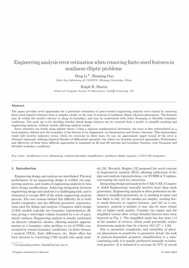
Integrating design and analysis for CAD/CAE (Comput-er Aided Engineering) typically involves more than meshgeneration. Engineering analysis is often performed on ide-alized or simplified geometries, as (i) meshing is easier andless likely to fail, (ii) the meshes are simpler, needing few-er small elements to capture features, and (iii) as a con-sequence, analysis is quicker; it may also be more robustdue to higher mesh quality. Consider the engine and thesimplified version after certain detailed features have beenremoved in Fig. 1. The simplified mesh has less than 1/4of the number of vertices, which could potentially reducedownstream analysis time by a factor of(1/4)3 = 1/64.
Due to geometric complexity, and variability of physi-cal phenomena in sensitivity to geometric detail, the taskof analysis-dependent geometry simplification is a time-consuming task; it is usually performed manually in indus-trial practice. It is estimated to account for 57% of overall
Preprint submitted to Elsevier 21 June 2012
(a) Original model (b) Simplified model
Fig. 1. An engine block and a simplified model.
analysis time, while mesh generation accounts for 23%; itis still not a fully solved problem [4,20,22,24].
In academia, geometry simplification for analysis hasbeen studied as a topic in both geometric modeling, andengineering analysis. The geometric modeling point of viewfocuses on geometric operations or algorithms to carry outsimplification, but usually ignores effects on analysis accu-racy. Criteria for guiding simplification are rooted in themodel’s geometry, and ignore physical properties and thephysical problem being solved. Such approaches cannot en-sure analysis will produce results of a desired accuracy.
Engineering analysis mainly focuses on the existence, u-niqueness, and accuracy of numerical solutions through apriori or a posteriori error estimates. Generally, two types oferrors have been studied. Numerical approximation errorsare incurred by computing discrete solutions for boundaryvalue problems [14]. Modeling errors are caused by usingsimplified mathematical equations to model physical phe-nomena [17]. Both approaches, however, assume that theunderlying geometry upon which analysis is performed isexact, while geometric simplification involves changes tothe underlying geometry.
The core issue in analysis-dependent geometry simplifi-cation is to quantitatively estimate the engineering analysiserror caused by defeaturing, or the modification error forshort. Solving an engineering analysis problem by utilizingsolutions of the defeatured model was first considered in1994 by Keller [13]. More recently, the work of Suresh etal [11,10,25] has made further progress on this topic, as haswork by Ferrandes et al [8] and Li et al [15]. However, theseprevious studies are mainly limited to linear problems, e.g.Poisson’s equation and linear elasticity, and are also lim-ited to features with (homogeneous) Neumann boundaryconditions (BCs).
Modification error estimation for nonlinear elliptic prob-lems was first studied in [16], which however only consid-ered Neumann BCs, using the dual weighted residual (D-WR) method. In this paper, we derive error estimates basedon adjoint theory, which can handle features with eitherNeumann BCs or Dirichlet BCs. Dirichlet BCs have beenlittle studied other than in [11], which only considers lin-ear Poisson equations with a special outer BC (solutionequal to zero). Here we build upon their idea in convert-ing goal-oriented modification error into a local quantitydefined over the boundary of the suppressed feature. This
idea was originally proposed for the Poisson equation; weextend it to the nonlinear elliptic case—see also Section 3.1.After this reformulation, we develop novel approaches forfeatures within the model’s interior or along its boundary.Our approach covers a wide range of situations, while theapproach in [11] for Neumann BC is essentially only appli-cable to a single internal feature, due to the use of exteriorapproximation, which is undefined for multiple features orfeatures lying on the boundary of an object.
Other related work on shape sensitivity analysis (SSA) [6]and topological sensitivity analysis (TSA) [23,2] mainly fo-cuses on infinitesimal geometry changes, while we considerfeatures of finite size. However, in this context, a rule-basedprinciple was also proposed by Russ et al [21] to simplifyCAD models to facilitate engineering analysis.
This paper proposes novel approaches for modificationerror estimation. Our methods cover a wide range of prac-tical industrial applications, many of which involve remov-ing finite-sized negative features within a model’s interi-or or on its boundary, with either Neumann or DirichletBCs, for nonlinear elliptic problems. The paper specificallyfocuses on semilinear elliptic equations, which represent awide range of physical phenomena, such as stationary heatconduction, wave propagation, and others [3]. Using a rig-orous mathematical derivation, the error is first expressedas a local quantity defined over the boundary of the fea-ture to be suppressed, by exploiting adjoint theory and alinearization approximation process. An approximate up-per bound for the modification error is obtained, and twoother heuristic numerical approaches are also presented forestimating the error, which are of use in practical computa-tions. These three different approaches are experimentallyvalidated for 2D and 3D internal and boundary features,with either Neumann or Dirichlet BCs.
The problem of estimating modification error is statedin Section 2. Concrete approaches for error estimation aredetailed in Section 3. Numerical experiments are presentedin Section 4, and conclusions are drawn in Section 5.
2. The problem of estimating modification error
Following [25,16], the problem of a posteriori goal-oriented modification error estimation is now described.
Unlike previous studies that focus on linear cases, we con-sider more challenging nonlinear elliptic engineering anal-ysis problems. We restrict our attention to a semilinearelliptic boundary value problem, namely equations wherethe nonlinearity involves the unknown function, but not itsderivatives. Semilinear elliptic equations are the first non-linear generalization of linear elliptic partial differential e-quations such as classical Laplace or Poisson equations [3].They have been studied for more than two hundred yearsand continue to attract researchers even today. Examplesthat fall into this important mathematical category can befound in a variety of contexts in physics, mechanics, engi-neering or life sciences, representing, for example, station-
2
ary heat conduction or wave conduction [3]. Nonlinearitymust be considered when slightly less restrictive assump-tions are made for modeling these physical phenomena. Ex-tension of the basic framework to other nonlinear ellipticproblems is discussed in Section 5.
The nonlinear problem is defined over an original com-plex geometry, whose corresponding field solutions are as-sumed hard to compute, or even intractable. By removinga set of features that form part of the original geometry, asimplified geometry is obtained, whose corresponding fieldsolutions are presumed to be much easier to determine. Ex-amples of an original complex geometry, and a correspond-ing simplified geometry, are shown in Fig. 1.
In this paper, we only study elimination of negative fea-tures (i.e. where material has been removed), which may becontained within the geometry’s interior or lie on its outerboundary. When only negative features exist, the originalgeometry is entirely contained within the simplified geom-etry, a useful property which no longer holds if positivefeatures are also present. Negative features are dominantin engineering components: many engineering componentsare created by removing materials from a blank such as ablock (again see Fig. 1). A heuristic approach to extendingthe approaches here to positive features could potentiallyfollow the ideas in [15]. The class of negative features con-sidered in this paper is quite general—they can be of finite-size, within the geometry’s interior or on its boundary, andsubject to either Neumann or Dirichlet BCs.
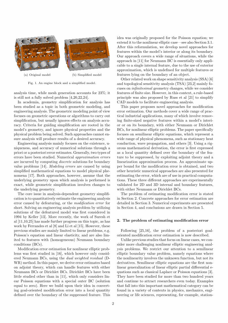
The problem is now described for a single internal fea-ture ω contained within the interior of the original geome-try Ω−ω in n-dimensional Euclidean space Rn, n = 2 or 3.See Fig. 2(a). Extension to boundary features or multiplefeatures is straightforward, and will be explained in Sec-tion 3.4. Removing ω from Ω− ω leaves a simplified geom-etry Ω as shown in Fig. 2(b). The boundary of Ω or ω isdenoted by ∂Ω or ∂ω respectively. As ω is fully containedwithin Ω, we have ∂(Ω − ω) = ∂Ω + ∂ω. We assume thatboth Ω−ω and Ω are bounded connected open regions withLipschitz boundaries [7], to ensure the validity of applica-tion of various classical results used in Section 3.
Over the original complex geometry Ω − ω, a nonlinearsecond order elliptic equation with solution u is defined:find the field solution u such that
Lu = f in Ω− ω,
Bu = b on ∂Ω,
Du = d or ud on ∂ω,
(1)
where L is an abstract nonlinear differential operator in aform as
Lu = −div(∇u) + g(u), (2)
for a continuous nonlinear function g(·). Boundary opera-tors B and D determine either Neumann or Dirichlet BCson the outer and inner boundaries ∂Ω and ∂ω. The lattermay be subject to either (a) Neumann or (b) Dirichlet BCs(if mixed, they can be considered separately): Du = d orud stands for
(a) Original geometry Ω − ω (b) Simplified geometry Ω
Fig. 2. Engineering analysis problems for original and simplified
geometries.
(a) ∂u/∂n = d, or (b) u = ud on ∂ω.
The problem and its BCs are characterized by the contin-uous functions f , b, d and ud.
Removing ω from Ω−ω leaves a simplified geometry withdifferent solution u0 satisfyingLu0 = f in Ω,
Bu0 = b on ∂Ω.(3)
The associated BCs Du = d over ∂ω have disappeared dueto the removal of the internal feature ω.
The geometric difference between the original geometryΩ − ω and its simplification Ω, essentially the differenceof the underlying computational domains, perturbs the en-gineering analysis problem defined over them. As in tra-ditional approaches to measuring approximation errors ormodeling errors, this solution difference, or modification er-ror for short, is described in terms of goal-oriented errorwhich records changes in quantities of particular engineer-ing or scientific interest. Compared to a global error mea-sure in an energy norm, goal-oriented error is much moreuseful in understanding effects on local values of interest,such as pointwise temperature or maximal stress over a cer-tain portion of the shape’s boundary.
Specifically, let us assume we are interested in a particu-lar local quantity of interest prescribed over a local regionS ∈ Ω− ω. In general form this may be written as follows:
Q(u) =
∫S
q(u) dS, (4)
where q(·) may be a linear or nonlinear function definedover S. We wish to estimate the difference in this localquantity caused by defeaturing, i.e.
δQ = e(Ω− ω,Ω) = Q(u)−Q(u0). (5)
It is permissible to use the solution u0 but we do not wantto explicitly use the solution u for the original geometry, asthis would defeat the purpose of defeaturing.
3. Error estimation
Our approach to estimating the modification error isbased on adjoint theory. The target quantity Q(u)−Q(u0)is reformulated as a local quantity defined over the bound-ary of the suppressed feature, by extending results for thePoisson equation in [11] to the nonlinear elliptic case. The
3
result, stated in Theorem 1, is the basis of the desired errorestimate but still involves unknown terms. Novel approxi-mate bounds for these unknown terms are then derived forfeatures with Neumann or Dirichlet BCs, and presented inTheorems 2 and 3. Following Theorem 1, we also proposetwo other novel heuristic approaches for providing modifi-cation error estimates in Section 3.4.
3.1. Error expressions based on adjoint theory
We first consider how to reformulate the target quantityQ(u) − Q(u0) as a local quantity defined over the bound-ary of the suppressed feature. The main steps are lineariza-tion and use of Green’s theorem with integration by parts.Specifically, we first build linear (approximate) governingequations of the solution error u−u0, and their adjoints, inLemma 1. The linearization process, in combination witha linear approximation to Q(u) − Q(u0), allows us to re-formulate the target modification error as a local quanti-ty defined over the boundary of the suppressed feature us-ing adjoint theory and Green’s theorem, following a similarprocedure to that used in [11].
We now briefly introduce adjoint theory. An adjoint solu-tion to an adjoint problem is defined with respect to an orig-inally defined prime problem. See, for example, (1) or (3).Adjoint solutions are typically used as weight factors in aposteriori goal-oriented error estimates in traditional FEapproximation [5] or modeling approximation [17]. Here,local residuals of the computed solutions are weighted bythe adjoint solutions, which measure the dependence of theerror on the local residual.
If the target functional Q(·) is linear, the adjoint formu-lation for a linear differential operator L in (1) may be de-scribed in a similar form to that for the prime problem byreplacing f (defined in (1)) by q (defined in (5)). Derivingsuch an adjoint operator for a nonlinear differential oper-ator L or target quantity Q(·) is not a trivial task, and isgenerally obtained using the primal-dual equivalence con-dition, as systematically studied by Giles and Suli [9].
For the specific nonlinear second order elliptic equationproblem in (1), the corresponding adjoint problem, withrespect to a linear or nonlinear target function Q(·), hasthe following form: find the solution p such that
−div(∇p) + g′(u)p = 0 in Ω− ω − S,
−div(∇p) + g′(u)p = q′(u) in S,
Bp = 0 on ∂Ω,
Dp = 0 on ∂ω.
(6)
Note that in the above adjoint formulation, the prime so-lution u is also involved in the first and second equations,and values of the BCs over the internal and outer bound-aries become zero. This occurrence of u only arises in non-linear cases, and makes the corresponding error estimationproblem much more challenging.
Similarly, the corresponding adjoint formulation for (3)is: find the solution p0 such that,
−div(∇p0) + g′(u0)p0 = 0 in Ω− S,
−div(∇p0) + g′(u0)p0 = q′(u0) in S,
Bp0 = 0 on ∂Ω.
(7)
In order to properly estimate the modification errorin (5), linear approximations to the governing equation ofboth the prime solution error e0 = u− u0, and the adjointerror ε0 = p − p0 are first built, which, together with alinearization of the local target quantity Q(u), linearizethe problem, as we now explain.
Firstly, approximate linear governing equations for e0, ε0are derived below.Lemma 1 The solution error e0 = u−u0 and adjoint errorε0 = p − p0 are approximately governed by the followinglinear equations with prescribed BCs,
−div(∇e0) + g′(u0)e0 = 0 in Ω− ω,
Be0 = 0 on ∂Ω,
De0 = d or ud −Du0 on ∂ω.
(8)
and −div(∇ε0) + g′(u0)ε0 = 0 in Ω− ω,
Bε0 = 0 on ∂Ω,
Dε0 = −Dp0 on ∂ω.
(9)
Proof: We only prove (8); (9) can be proved similarly.Thevalidity of the BCs over the outer and internal boundariesfollows directly. We now prove the first equation in (8) overthe interior Ω− ω. From Eqs. (1) and (3),
Lu = −div(∇u)+g(u) = f, Lu0 = −div(∇u0)+g(u0) = f.
Subtracting the above two equations, we have
Lu− Lu0 = −div(∇(u− u0)) + (g(u)− g(u0)) = 0.
The Taylor expansion of g(u)−g(u0) when u−u0 is small is
g(u)− g(u0) = g′(u0)(u− u0) +O(u− u0).
Discarding the higher order term gives
Lu− Lu0 = −div(∇(u− u0)) + g′(u0)(u− u0) = 0.
Hence, as required,
−div(∇e0) + g′(u0)e0 = 0.
2
From the above lemma, the modification error δQ =Q(u)−Q(u0) can be approximated via a linearization pro-cess, using adjoint theory. Specifically, after finding a linearapproximation to Q(u) − Q(u0), the adjoint solution canthen be introduced into the error expression. Then, follow-ing a similar procedure to one in [11], performing integra-tion by parts twice, and utilizing the relation between solu-tions u and u0 (they are governed by the same differentialoperator within the model interior and constrained by the
4
same BCs except on the internal feature boundary), themodification error can be ultimately expressed as a localquantity defined over the internal feature boundary. Thisis stated in the following theorem, followed by its proof.Theorem 1 The modification error δQ in (5) for an in-ternal feature ω can be estimated as a local quantity definedover the feature boundary ∂ω using adjoint solutions whenu− u0 is small:
δQ ≈ −∫∂ω
∇p0 · n(u− u0) dS +
∫∂ω
p0∇(u− u0) · n dS.
(10)Proof: Denote Ω = Ω − ω for simplicity. Using Taylor ex-pansion, a linear approximation to the target quantity δQcan be obtained when u− u0 is small:
δQ=
∫S
(q(u)− q(u0)) dV
=
∫S
(q′(u0)(u− u0) +O(u− u0)) dV.
Discarding the higher order term O(u− u0), and takinginto account (7), we have
δQ≈−∫S
(div(∇p0)− g′(u0)p0)(u− u0) dV
−∫
Ω−S(div(∇p0)− g′(u0)p0)(u− u0) dV.
After performing two steps of integration by parts, we get
δQ ≈ −∫∂Ω
∇p0 · n(u− u0) dS +
∫Ω
∇p0 · ∇(u− u0) dV
+
∫Ω
g′(u0)p0(u− u0)) dV
= −∫∂Ω
∇p0 · n(u− u0) dS +
∫∂Ω
p0∇(u− u0) · n dS
−∫
Ω
(div(∇(u− u0))p0 − g′(u0)p0(u− u0)) dV.
From (8), the third term in the above equation vanishes, so
A similar procedure shows that Theorem 1 also holdstrue for the case of a boundary feature. Later results in thispaper based on Theorem 1 do not explicitly assume internalfeatures, and thus also hold true for boundary features. Weparticularly note that the approximate equality in (10) onlyarises due to linearization of Q(u) −Q(u0) in (11), and ofthe governing equations for e0 and ε0. The equality in (10)holds exactly if L is linear and if Q(u) is linear.
Theorem 1 reformulates the modification error in termsof a local quantity defined over the feature boundary ∂ωusing adjoint solutions. This estimate cannot yet be com-puted directly since it still involves the unknown full solu-tion u. Consider (10). For Neumann BC on ∂ω, the valueof ∇(u−u0) ·n in the second term is known, and the valueof u− u0 in the first term is unknown. On the other hand,for Dirichlet BC on ∂ω, the value of u− u0 in the first ter-m is known, and value of (u− u0) · n in the second term isunknown. In either case, one term in (10) is unknown andneeds to be further estimated, which we now consider.
Before we start, three norms are introduced assumingthat g′(v) are always positive. These arethe energy norm:
‖v‖E =√α(v, v), forα(u, v) =
∫Ω−ω
(∇u·∇v+g′(u0)uv) dV,
(12)the Lp-norm:
‖v‖Lp(Ω) = (
∫∂ω
|v|p dS)1/p,
and the Hk-norm:
‖v‖Hk(Ω) = (∑|κ|≤k
‖Dκv‖2L2(Ω))1/2,
where κ is a multi-index, and
Dκv =∂|κ|v
∂xκ11 . . . ∂xκn
n.
3.2. Error estimation for features with Neumann BCs
In this section, we give a novel approach to further esti-mate the quantities in (10) when the internal feature ω hasNeumann BCs, ∇u ·n = d over ∂ω. In this case, the secondterm on the right hand side of (10) is known:∫
∂ω
p0∇(u− u0) · n dS =
∫∂ω
(d− d0)p0 dS (13)
for d0 = ∇u0 · n. We only need to estimate the first, un-known, term, as below.Theorem 2 When feature ω has Neumann BC, specifical-ly∇u ·n = d on ∂ω, the modification error in (5) is approx-imately bounded below by
|δQ| ≤ |∫∂ω
(d−d0)p0 dS|+C2N‖∇p0·n‖L2(∂ω)‖d−d0‖L2(∂ω),
(14)where d0 = ∇u0 · n, and CN is a constant only dependenton the geometry of Ω−ω, whose practical computation willbe discussed in Section 3.4.
5
Proof: We first estimate the energy norm of the solutionerror e0 = u − u0, and then use it to estimate δQ basedon (10).
Multiplying the first line of (9) by a functional v andperforming integration by parts gives the following weakform for e0: find solution e0 ∈ V such that∫
Ω−ω(∇e0 · ∇v + g′(u0)e0v) dV =
∫∂ω
(d− d0)v ds, v ∈ V,
(15)where V is the appropriate Sobolev space [7].
From the trace theorem (see [7]) and the equivalence ofthe H1 norm and the energy norm, a constant CN existssuch that
Thus, as e0 = u− u0, the first unknown term in (10) maybe estimated to be no more than the quantity below:
|∫∂ω
∇p0 · ne0 dS| ≤ ‖∇p0 · n‖L2(∂ω)‖e0‖L2(∂ω)
≤ ‖∇p0 · n‖L2(∂ω)CN‖e0‖E≤ C2
N‖∇p0 · n‖L2(∂ω)‖d− d0‖L2(∂ω).
By further taking into account Eqs. (13) and (10), the tri-angle inequality gives Theorem 2. 2
3.3. Error estimation for features with Dirichlet BCs
We next give a novel approach to further estimate thequantities in (10) when the internal feature ω has DirichletBCs, u = ud over ∂ω. In this case, the first term on theright side of (10) is known, so
−∫∂ω
∇p0 ·n(u−u0) dS = −∫∂ω
∇p0 ·n(ud−u0) dS, (17)
and we only need to further estimate the unknown, second,term. As a result, estimation of the modification error inthis case is given below.Theorem 3 When feature ω has Dirichlet BC, specificallyu = ud on ∂ω, the modification error in (5) is approximatelybounded below by:
|δQ| ≤ |∫∂ω
∇p0 · n(ud − u0) dS|
+CD‖p0‖L2(∂ω)(‖ud − u0‖L2(∂ω) + ν(e)), (18)
where ν(e) = ‖e‖L2(Ω−ω) +C0‖div(∇e)− g′(u0)e‖L2(Ω−ω),e is any function satisfying (19), and C0, CD are constantsonly dependent on the geometry of Ω − ω, whose practicalcomputation will be discussed in Section 3.4.Proof: This follows the proof for Neumann BC, but is morechallenging. A strategy of reformulating the Dirichlet ter-m with respect to e0 over the internal feature boundary∂ω using the source term of its governing equation is ap-plied. We first consider estimation of ‖e0‖L2(Ω−ω). Choosea function e satisfying the following BCs:
Be = 0 on ∂Ω, e = ud − u0 on ∂ω. (19)
Setting e = e0 − e, (8) gives the following equation for e:−div(∇e) + g′(u0)e = div(∇e)− g′(u0)e in Ω− ω,
Be = 0 on ∂Ω,
e = 0 on ∂ω.
H2-regularity of elliptic operators (see [7]) gives
By further taking into account Eqs. (17) and (10), the tri-angle inequality gives Theorem 3. 2
Function e can be obtained via interpolation techniques,such as radial basis functions, with a goal to minimize ν(e),or alternatively, by solving a simple linear boundary valueproblem, for example, the Poisson equation, over a coarsemesh for Ω − ω with prescribed BCs in (19). The latter isemployed in this paper for ease of implementation with asource term equal to 0.
6
3.4. Discussion
We now consider several further practical issues: settingsfor the constants CN , C0, CD discussed earlier, cases withmultiple features, and heuristic approaches to estimatingmodification error.
3.4.1. Constant settingsPractical use of the results in Theorems 2 and 3 for es-
timating modification error still depends on properly set-ting the constants CN , C0, CD. Essentially, no theoretical-ly sound approach exists for finding such constants excep-t in a very few special cases. A previous approach in [26]also utilized similar constants to simplify linear elasticityanalysis of perforated materials, but no explicit approachwas given for constant setting. In our problem, obtainingexact or tight values of CN , C0, CD is not very essential, s-ince the final modification error estimate also depends onthe known terms over the feature’s boundary (see Eqs. (14)and (18)), which usually account for a larger contributionto the overall estimated error. We now discuss a practicalnumerical approach for fining values for these constants.
The derivation of Theorem 2 shows that CN is best setso that (16) become an equality for solution error v = e0,that is,
CN =‖e0‖L2(∂ω)
‖e0‖E. (24)
However, the solution error e0 = u − u0 is actually un-known. The trace theorem tell us that CN only depends onthe geometry of Ω−ω. Taking into account that (16) is sat-isfied for all v ∈ V , we may thus use the space spanned bythe computed prime and adjoint solutions u0, p0 as a basespace, and in practice set CN to be
CN = maxs
‖(su0 ± p0/s)‖L2(∂ω)
‖su0 ± p0/s‖E.
This maximal value can be estimated by sampling the pa-rameter s in the range 0 to 1 with say 100 equally spacedsteps.
In a similar way, the constants C0, CD may be practicallydetermined using
C0 = maxs
‖su0 ± p0/s− e‖L2(Ω−ω)
‖div(∇e)− g′(u0)e‖L2(Ω−ω),
or simply taken as 1 in 2D cases, and
CD = maxs
‖∇(su0 ± p0/s)‖L2(∂ω)
‖(su0 ± p0/s)‖L2(Ω−ω) + ‖ud − u0‖L2(Ω−ω).
3.4.2. Multiple featuresThe results in Theorems 2 and 3 presume a single fea-
ture. We now consider multiple features. Suppose ωi, i =1, . . . , n, are a set of features to be suppressed within a ge-ometry Ω. Let Ω = Ω−Σiωi be the original geometry, andΩi = Ω − ωi be the geometry containing a single featureωi. The results in Theorems 1–3 do not make any assump-tion that only a single feature is present, and can thus be
applied directly to cases with multiple features. Specifical-ly, the modification error caused by removing all these fea-tures Ωi is simply their summation, that is,
e(Ω,Ω) = Σie(Ωi,Ω).
This allows efficient handling of multiple features as only asingle engineering analysis is needed on the fully simplifiedgeometry Ω.
3.4.3. Other heuristic approachesUtilizing the results in Theorems 2 and 3 involves proper
estimation of the involved constants, so we also suggestsome alternative heuristic approaches based on Theorem 1.While these are not particularly theoretically sound, theydo provide alternative, simple, practical approaches.
Consider the two terms in (10) in Theorem 1, for eitherNeumann or Dirichlet BC over ∂ω. In either case, one ter-m is known, and the other unknown. Estimates of the un-known terms essentially depend on estimates of u − u0 or∇(u− u0) · n along ∂ω.
A heuristic approach to providing them can be basedon a local computation strategy, building a local regionΘ surrounding ω, with a corresponding solution e0 as anapproximation to e0 = u−u0, assuming that u = u0 along∂Θ. Taking into account Eqs. (1) and (3) gives the followingequation for e0 = u− u0:
Le0 = 0 in Θ− ω,
Be0 = 0 on ∂Θ,
De0 = d (or ud)−Du0 on ∂ω,
(25)
Computing e0 only involves a small local region Θ, andis thus much cheaper to compute than computing e0 overΩ−ω. Once a solution e0 has been found, the modificationerror can be estimated using Theorem 1. Specifically, forNeumann BCs on ∂ω,
δQ ≈ −∫∂ω
∇p0 · ne0 dS +
∫∂ω
p0(d− d0) dS, (26)
while for Dirichlet BCs on ∂ω,
δQ ≈ −∫∂ω
∇p0 · n(ud − u0) dS +
∫∂ω
p0∇e0 · n dS. (27)
Since the expression in Theorem 10 only depends on thevalue of e0 along ∂ω, the particular choice of Θ does notgreatly change the value of the final estimated errors, andwe can thus arbitrarily select Θ in practice. The solutione0 can then be computed numerically via a traditional FEmethod. A similar approach based on local computationwas applied in [8] to estimate modification error measuredin the global energy norm during linear elasticity analysis.Unlike our approach that only involves the estimated valueon the boundary ∂ω, the approach in [8] estimated valuesover the whole model.
Another simple heuristic strategy to error estimation isto simply discard the unknown term in (10), resulting inerror estimates
7
δQ ≈∫∂ω
p0(d− d0) dS. (28)
for Neumann BCs, and
δQ ≈ −∫∂ω
∇p0 · n(ud − u0) dS. (29)
for Dirichlet BCs. The above result for Neumann BCs isconsistent with earlier results in [16] based on a differentapproach; the suggestion for Dirichlet BC is novel.
3.5. Extension to other nonlinear elliptic problems
The proposed approach can also be extended to nonlin-ear second-order elliptic problems. However, concrete ex-pressions for error estimation are very problem-dependent,and need to be derived for each specific case.
Specifically, a nonlinear second-order elliptic problemcan be represented in the following form over Ω− ω:
Lu =∑i
ai(x)∂2u
∂2xi+ g(∇u, u) (30)
for continuous functions ai(·) and nonlinear continuousfunction g(·, ·).
Following a similar procedure of linear approximationand integration by parts, a result corresponding to Theo-rem 1 can also be derived for this case without difficulty.This result can be guaranteed for any nonlinear second-order elliptic problem without requiring any additionalproperties, as long as the solution exists. Further error es-timation, as done in Theorems 2 and 3, are however highlydependent on the particular form of Lu. For example, ifg(u) = −u3, the solution uniqueness and existence are nolonger guaranteed and the energy norm in (12) is not prop-erly defined. Correspondingly, the error estimates have tobe re-derived based on the result in Theorem 1. The prob-lem of linear elasticity or nonlinear elasticity can be seenas a vector form of (30) and thus falls into the scope of theabove discussion.
4. Experimental results
The above approach to estimating modification errorshas been implemented using COMSOL [1], a commercialfinite-element based CAD/CAE system. Taking specifical-ly g(u) = u3, we have tested various cases: 2D internal andboundary features, 3D features, and multiple features witheither Neumann or Dirichlet BCs, the features having var-ious sizes and locations.
The accuracy of an error estimate is usually measured interms of effectivity index, or EI for short, the ratio betweenthe estimated error e and the ground truth error E, that is,
I = e/E.
An EI between 0.5 and 2.0 is often taken as reasonable forerror measured in a global energy norm. However, for goal-oriented error estimation as studied in this paper, obtaining
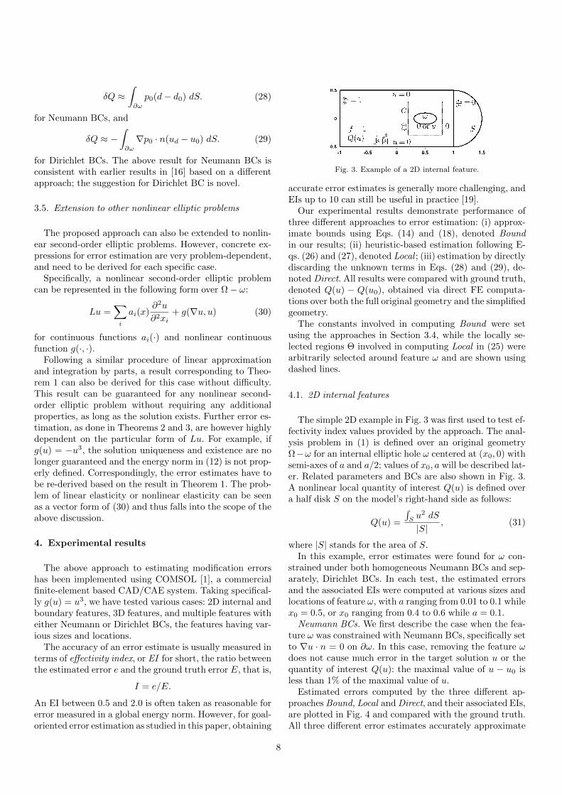
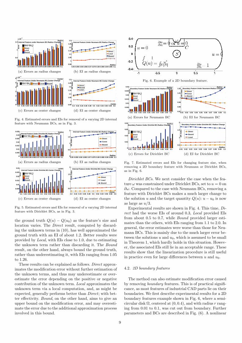
Fig. 3. Example of a 2D internal feature.
accurate error estimates is generally more challenging, andEIs up to 10 can still be useful in practice [19].
Our experimental results demonstrate performance ofthree different approaches to error estimation: (i) approx-imate bounds using Eqs. (14) and (18), denoted Boundin our results; (ii) heuristic-based estimation following E-qs. (26) and (27), denoted Local ; (iii) estimation by directlydiscarding the unknown terms in Eqs. (28) and (29), de-noted Direct. All results were compared with ground truth,denoted Q(u) − Q(u0), obtained via direct FE computa-tions over both the full original geometry and the simplifiedgeometry.
The constants involved in computing Bound were setusing the approaches in Section 3.4, while the locally se-lected regions Θ involved in computing Local in (25) werearbitrarily selected around feature ω and are shown usingdashed lines.
4.1. 2D internal features
The simple 2D example in Fig. 3 was first used to test ef-fectivity index values provided by the approach. The anal-ysis problem in (1) is defined over an original geometryΩ−ω for an internal elliptic hole ω centered at (x0, 0) withsemi-axes of a and a/2; values of x0, a will be described lat-er. Related parameters and BCs are also shown in Fig. 3.A nonlinear local quantity of interest Q(u) is defined overa half disk S on the model’s right-hand side as follows:
Q(u) =
∫Su2 dS
|S|, (31)
where |S| stands for the area of S.In this example, error estimates were found for ω con-
strained under both homogeneous Neumann BCs and sep-arately, Dirichlet BCs. In each test, the estimated errorsand the associated EIs were computed at various sizes andlocations of feature ω, with a ranging from 0.01 to 0.1 whilex0 = 0.5, or x0 ranging from 0.4 to 0.6 while a = 0.1.
Neumann BCs. We first describe the case when the fea-ture ω was constrained with Neumann BCs, specifically setto ∇u · n = 0 on ∂ω. In this case, removing the feature ωdoes not cause much error in the target solution u or thequantity of interest Q(u): the maximal value of u − u0 isless than 1% of the maximal value of u.
Estimated errors computed by the three different ap-proaches Bound, Local and Direct, and their associated EIs,are plotted in Fig. 4 and compared with the ground truth.All three different error estimates accurately approximate
Fig. 5. Estimated errors and EIs for removal of a varying 2D internal
feature with Dirichlet BCs, as in Fig. 3.
the ground truth Q(u) − Q(u0) as the feature’s size andlocation varies. The Direct result, computed by discard-ing the unknown terms in (10), has well approximated theground truth with an EI of about 1.2. Better results wereprovided by Local, with EIs close to 1.0, due to estimatingthe unknown term rather than discarding it. The Boundresult, on the other hand, always bound the ground truth,rather than underestimating it, with EIs ranging from 1.05to 1.26.
These results can be explained as follows. Direct approx-imates the modification error without further estimation ofthe unknown terms, and thus may underestimate or over-estimate the error depending on the positive or negativecontribution of the unknown term. Local approximates theunknown term via a local computation, and, as might beexpected, generally performs better than Direct ; with bet-ter effectivity. Bound, on the other hand, aims to give anupper bound on the modification error, and may overesti-mate the error due to the additional approximation processinvolved in this bound.
Boundary Feature Under Dirichlet BC: Radius Change
Direct
Bound
Local
(d) EI for Dirichlet BC
Fig. 7. Estimated errors and EIs for changing feature size, whenremoving a 2D boundary feature with Neumann or Dirichlet BCs,
as in Fig. 6.
Dirichlet BCs. We next consider the case when the fea-ture ω was constrained under Dirichlet BCs, set to u = 0 on∂ω. Compared to the case with Neumann BCs, removing afeature with Dirichlet BCs makes a much larger change tothe solution u and the target quantity Q(u): u− u0 is nowas large as u/3.
Experimental results are shown in Fig. 4. This time, Di-rect had the worse EIs of around 0.3, Local provided EIsfrom about 0.5 to 0.7, while Bound provided larger esti-mates than the others, with EIs ranging from 1.1 to 2.0. Ingeneral, the error estimates were worse than those for Neu-mann BCs. This is mainly due to the much larger error be-tween the solutions u and u0, which is assumed to be smallin Theorem 1, which hardly holds in this situation. Howev-er, the associated EIs still lie in an acceptable range. Theseresults show that the linearization procedure is still usefulin practice even for large differences between u and u0.
4.2. 2D boundary features
The method can also estimate modification error causedby removing boundary features. This is of practical signifi-cance, as most features of industrial CAD parts lie on theirboundaries. We first describe experimental results for a 2Dboundary features example shown in Fig. 6, where a semi-circular disk Ω, centered at (0, 0.4), and with radius r rang-ing from 0.01 to 0.1, was cut out from boundary. Furtherparameters and BCs are described in Fig. (6). A nonlinear
9
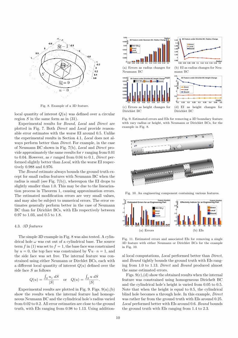
Fig. 8. Example of a 3D feature.
local quantity of interest Q(u) was defined over a circularregion S in the same form as in (31).
Experimental results for Bound, Local and Direct areplotted in Fig. 7. Both Direct and Local provide reason-able error estimates with the worse EI around 0.5. Unlikethe experimental results in Section 4.1, Local does not al-ways perform better than Direct. For example, in the caseof Neumann BC shown in Fig. 7(b), Local and Direct pro-vide approximately the same results for r ranging from 0.01to 0.04. However, as r ranged from 0.04 to 0.1, Direct per-formed slightly better than Local, with the worse EI respec-tively 0.988 and 0.976.
The Bound estimate always bounds the ground truth ex-cept for small radius features with Neumann BC when theradius is small (see Fig. 7(b)), whereupon the EI drops toslightly smaller than 1.0. This may be due to the lineariza-tion process in Theorem 1, causing approximation errors.The estimated modification errors are very small values,and may also be subject to numerical errors. The error es-timates generally perform better in the case of NeumannBC than for Dirichlet BCs, with EIs respectively between0.97 to 1.03, and 0.5 to 1.8.
4.3. 3D features
The simple 3D example in Fig. 8 was also tested. A cylin-drical hole ω was cut out of a cylindrical base. The sourceterm f in (1) was set to f = 1, the base face was constrainedby u = 0, the top face was constrained by ∇u · n = 1, andthe side face was set free. The internal feature was con-strained using either Neumann or Dirchlet BCs, each witha different local quantity of interest Q(u) defined over theside face S as follows
Q(u) =
∫Suz dS
|S|or Q(u) =
∫Su dS
|S|.
Experimental results are plotted in Fig. 9. Figs. 9(a),(b)show the results when the internal feature had homoge-neous Neumann BC and the cylindrical hole’s radius variedfrom 0.02 to 0.2. All error estimaties are close to the groundtruth, with EIs ranging from 0.98 to 1.13. Using addition-
0.02 0.04 0.06 0.08 0.1 0.12 0.14 0.16 0.18 0.20
0.005
0.01
0.015
0.02
0.025
0.03 Radius
Err
or 3D Feature under Neumann BC: Radius Change
Q(u)−Q(u0)
DirectLocalBound
(a) Errors as radius changes forNeumann BC
0.02 0.04 0.06 0.08 0.1 0.12 0.14 0.16 0.18 0.2
0.98
1
1.02
1.04
1.06
1.08
1.1
1.12
Radius
Eff
. In
dex
3D Feature under Dirichlet BC: Radius Change
DirectLocalBound
(b) EI as radius changes for Neu-mann BC
0.1 0.15 0.2 0.25 0.3 0.35 0.4 0.45 0.50
0.002
0.004
0.006
0.008
0.01
0.012
0.014 Height
Err
or
3D Feature under Dirichlet BC:Height Change
Q(u)−Q(u0) Direct Local Bound
(c) Errors as height changes for
Dirichlet BC
0.1 0.15 0.2 0.25 0.3 0.35 0.4 0.45 0.50
0.5
1
1.5
2
2.5
Height
Eff
. In
dex
3D Feature under Dirichlet BC:Height Change
DirectLocalBound
(d) EI as height changes for
Dirichlet BC
Fig. 9. Estimated errors and EIs for removing a 3D boundary featurewith vary radius or height, with Neumann or Dirichlet BCs, for the
example in Fig. 8.
Fig. 10. An engineering component containing various features.
Fig. 11. Estimated errors and associated EIs for removing a single3D feature with either Neumann or Dirichlet BCs for the example
in Fig. 10.
al local computations, Local performed better than Direct,and Bound tightly bounds the ground truth with EIs rang-ing from 1.0 to 1.13. Direct and Bound produced almostthe same estimated errors.
Figs. 9(c),(d) show the obtained results when the internalfeature was constrained using homogeneous Dirichelt BCand the cylindrical hole’s height is varied from 0.05 to 0.5.Note that when the height is equal to 0.5, the cylindricalblind hole becomes a through hole. In this example, Directwas rather far from the ground truth with EIs around 0.25.Local performed better with EIs around 0.6. Bound boundsthe ground truth with EIs ranging from 1.4 to 2.3.
10
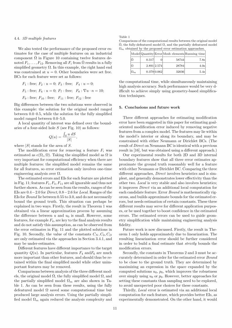
4.4. 3D multiple features
We also tested the performance of the proposed error es-timates for the case of multiple features on an industrialcomponent Ω in Figure 10 containing twelve features de-noted F1, . . . , F12. Removing all Fi from Ω results in a fullysimplified geometry Ω. In this example, the right hand endwas constrained at u = 0. Other boundaries were set free.BCs for each feature were set as follows:
F1 : free; F2 : u = 0; F3 : free; F4 : u = 0;
F5 : free; F6 : u = 0; F7 : free; F8 : ∇u · n = 10;
F9 : free; F10 : free; F11 : free; F12 : free
Big differences between the two solutions were observed inthis example: the solution for the original model rangedbetween 0.0–0.5, while the solution for the fully simplifiedmodel ranged between 0.0–5.0.
A local quantity of interest was defined over the bound-aries of a four-sided hole S (see Fig. 10) as follows:
Q(u) =
∫Su dS
|S|,
where |S| stands for the area of S.The modification error for removing a feature Fi was
estimated as e(Ωi,Ω). Taking the simplified model as Ω isvery important for computational efficiency when there aremultiple features: the simplified model remains the samefor all features, so error estimation only involves one-timeengineering analysis over Ω.
The estimated errors and EIs for each feature are plottedin Fig. 11; features F1, F3, F11 are all ignorable and thus notfurther shown. As can be seen from the results, ranges of theEIs are 0.4−2.0 for Direct, 0.8−2.6 for Local. Ranges of theEIs for Bound lie between 0.55 to 3.0, and do not necessarilybound the ground truth. This situation can perhaps beexplained in two ways. Firstly, the result in Theorem 1 wasobtained via a linear approximation process by assumingthe difference between u and u0 is small. However, somefeatures, for example F4, are key to the final analysis resultsand do not satisfy this assumption, as can be observed fromthe error estimates in Fig. 11 and the plotted solutions inFig. 10. Secondly, the value of the constants CN , C0, CDare only estimated via the approaches in Section 3.4.1, andmay be under-estimates.
Different features have different importance to the targetquantity Q(u). In particular, features F4 andF6 are muchmore important than other features, and should thus be re-tained within the final simplified model while other unim-portant features may be removed.
Comparisons between analysis of the three different mod-els, the original model Ω, the fully simplified model Ω, andthe partially simplified model Ωm are also shown in Ta-ble 1. As can be seen from these results, using the fullydefeatured model Ω saved some computational time butproduced large analysis errors. Using the partially simpli-fied model Ωm again reduced the analysis complexity and
Table 1Comparisons of the computational results between the original model
Ω, the fully-defeatured model Ω, and the partially defeatured model
Ωm obtained by the proposed error estimation approaches.
Model Quantity Error Mesh elements Running time
Ω 0.317 0 58744 7.8s
Ω 2.891 2.574 28784 4.0s
Ωm 0.379 0.062 32036 5.4s
the computational time, while simultaneously maintaininghigh analysis accuracy. Such performance would be very d-ifficult to achieve simply using geometry-based simplifica-tion techniques.
5. Conclusions and future work
Three different approaches for estimating modificationerror have been suggested in this paper for estimating goal-oriented modification error induced by removing negativefeatures from a complex model. The features may lie withinthe model’s interior or along its boundary, and may beconstrained with either Neumann or Dirichlet BCs. (Theresult of Direct on Neumann BC is identical with a previousresult in [16], but was obtained using a different approach.)
Our experimental results for both 2D and 3D internalboundary features show that all three error estimates ap-proximate the ground truth reasonably well for a featurewith either Neumann or Dirichlet BC. Comparing the threedifferent approaches, Direct involves heuristics and is sim-plest, and generally demonstrates lower effectivity than theother two. Local is very stable and also involves heuristics;it improves Direct via an additional local computation foreach candidate feature. Error Bound is mathematically rig-orous, and builds approximate bounds for the estimated er-rors, but needs estimation of certain constants. These threedifferent results may serve for different application purpos-es, or be used together to boost confidence in the estimatederrors. The estimated errors can be used to guide geom-etry simplification while maintaining engineering analysisfidelity.
Future work is now discussed. Firstly, the result in The-orem 1 only holds approximately due to linearization. Theresulting linearization error should be further consideredin order to build a final estimate that strictly bounds themodification errors.
Secondly, the constants in Theorems 2 and 3 must be ac-curately determined in order for the estimated error Boundto be close to the ground truth. They are determined bymaximizing an expression in the space expanded by thecomputed solutions u0, p0, which improves the robustnessover simply using u0 or p0. However, better approaches forsetting these constants than sampling need to be explored,to avoid unexpected poor choices for these constants.
Thirdly, Local error is estimated via an additional localcomputation for each feature, which provides better EIs, asexperimentally demonstrated. On the other hand, it would
11
be an improvement to avoid heuristics. Theoretically rigor-ous approaches need to be further developed to optimallyselect the region used, or to explore the effect of region s-election on the final estimated errors. Furthermore, by ap-propriately setting the values of u along the boundary Θ,we may build an error approximation with verified conver-gence, or even strict lower and upper bounds on the esti-mated errors. Extending the approach in [13] may achievethis. Note that the proposed approach of local region selec-tion is different from multigrid methods or domain decom-position methods in that the former aim to properly esti-mate the modification error, which may be small or large,while the latter aim to find the target exact solution, ig-noring numerical approximation error, via local iterativecomputation strategies.
Fourthly, the approach relies on the original model be-ing contained within the simplified model, which does nothold in the case of positive features. A heuristic approachvia local solution extension has been proposed in [15] to re-solve this issue, which can also be applied here for cases ofpositive features. However, this approach still lacks a rigor-ous theoretical verification, and deserves further researcheffort.
Lastly, applying the proposed approach to generating asimplified geometric model with engineering analysis errorcontrol is a non-trivial task and needs to be further ex-plored. More work is needed on estimation of the engineer-ing analysis error caused by removing multiple features,which may interact, and on optimal selection of features forremoval. Furthermore, geometric approaches are needed toautomatically detect candidate features to be suppressed,and to suppress them, in cases both where feature infor-mation is part of the model, and where it must be deducedfrom the geometry alone. An approach towards this goalcan be found in [20].
Acknowledgements
The work described in this paper was partially support-ed by the National Basic Research Program of China (No.2011CB302400), the NSF of China (No. 61103103). Wethank Dr. Kai Zhang for his helpful discussions on themanuscript, and Junzhe Zheng for implementing the tests.
Journal of Computing and Information Science in Engineering,11(2):021005–1:13, 2011.
[23] J. Sokolowski and A. Zochowski. On topological derivative inshape optimization. SIAM Journal of Control Optimization,37(4):1251–1272, 1999.
[24] A. Thakur, A. Banerjee, and S. Gupta. A survey of CAD
model simplification techniques for physics-based simulationapplications. Computer-Aided Design, 41(2):65–80, 2009.
[25] I. Turevsky, S. Gopalakrishnan, and K. Suresh. Defeaturing:A posteriori error analysis via feature sensitivity. InternationalJournal for Numerical Methods in Engineering, 76(9):1379–1401,
2008.[26] K. Vemaganti. Modelling error estimation and adaptive
modelling of perforated materials. International Journal forNumerical Methods in Engineering, 59(12):1587–1604, 2004.