ENGLISH AGRICULTURAL OUTPUT AND LABOUR PRODUCTIVITY, …

ENGLISH AGRICULTURAL OUTPUT AND LABOUR PRODUCTIVITY, 1250-

1850: SOME PRELIMINARY ESTIMATES

Alexander Apostolides, University of Warwick, [email protected] Broadberry, University of Warwick, [email protected]

Bruce Campbell, Queen’s University Belfast, [email protected] Overton, University of Exeter, [email protected]

Bas van Leeuwen, University of Warwick, [email protected]

26 November 2008File: AgricLongRun4.doc

Abstract: This paper provides annual estimates of English agricultural output and labourproductivity during the period 1250-1850, based on manorial records from the medievalperiod, probate inventories from the early modern period and farm accounts from themodern period. Agricultural labour productivity increased sharply in the immediateaftermath of the Black Death and remained at this higher level for the rest of the medievalperiod. There was a further increase between the mid-fifteenth and mid-sixteenthcenturies, with labour productivity remaining at this higher level until the earlyeighteenth century. These pre-modern increases in labour productivity were achievedwithout a substantial increase in output per unit of land. The early eighteenth century sawthe start of a continuous upward trend in both agricultural labour productivity and landproductivity.

Acknowledgements: This paper forms part of the project “Reconstructing the NationalIncome of Britain and Holland, c.1270/1500 to 1850”, funded by the Leverhulme Trust,Reference Number F/00215AR.

mailto:[email protected]





2

I. INTRODUCTION

Two very contrasting view of the development of the English economy between the late

medieval period and the Industrial Revolution co-exist. One view, which has been based

largely on real wage evidence, paints a bleak picture of long run stagnation from the late

thirteenth century to the middle of the nineteenth century, albeit with quite large

fluctuations over sustained periods (Phelps Brown and Hopkins, 1981). This view has

recently been supported by Clark (2005), who provides a real wage series which shows

less extreme fluctuations than that of Phelps Brown and Hopkins, but leaves the trend

unchanged. Furthermore, Clark (2007a) adds new time series for land rents and capital

income to arrive at a picture of long run stagnation in GDP per head. This view sits

uneasily with a second view, based largely on estimates of wealth and the appearance of

new products, which appears to show modest but sustained growth of living standards

between the middle ages and the Industrial Revolution (Overton, Whittle, Dean and

Haan, 2004; de Vries, 1994).

These two very different views of the long run development of the English

economy have been able to co-exist because of the absence of reliable and empirically

well grounded estimates of the output and labour productivity of the English economy

over much of this period. This paper forms part of a project to reconstruct the national

income of Britain and Holland between the late thirteenth century and the mid-nineteenth

century. Here, we focus on agriculture, the largest sector of the economy for much of the

period under consideration, providing annual estimates of agricultural output for England

3

over the long period 1270-1850 and putting them together with estimates of the

agricultural labour force to track the path of agricultural labour productivity.

The approach builds on the pathbreaking study of Overton and Campbell (1996),

which tracked long run trends in agricultural output and labour productivity, but was

restricted to estimates for a small number of benchmark years. To provide annual

estimates, we rely heavily on three data sets assembled for the medieval, early modern

and modern periods. For the medieval period, we analyse the Medieval Accounts

Database assembled by Campbell (2000; 2007), drawing upon the archival labours of a

number of other historians, including David Farmer, John Langdon and Jan Titow. The

information on arable yields and animal stocking densities is taken largely from manorial

accounts, but is supplemented by information on the non-manorial sector from tithes. For

the early modern period, we use the probate inventory database assembled by Overton,

Whittle, Dean and Hann (2004), which provides indirect estimates of arable yields and

animal stocking densities from the valuation of the assets left by farmers. From the early

eighteenth century on, we make use of the database on farm accounts assembled by

Turner, Beckett and Afton (2001).

The trends that emerge from these three datasets are broadly consistent, which

increases our confidence in the underlying data. Furthermore, the national accounting

perspective suggests other tests which can be conducted to demonstrate consistency.

4

The paper proceeds as follows. Section II provides a brief introduction to the main

data sources for the three periods. Estimates of output for the arable sector are then given

in section III, followed by estimates of pastoral sector output in section IV. The arable

and pastoral outputs are then combined in section V to provide estimates of overall

agricultural output. The index of overall agricultural output is then combined with

estimates of population and the agricultural labour force in section VI to provide an

overview of the path of agricultural labour productivity. Estimates from the output side

are then cross-checked against estimates from the income side and per capita

consumption of calories in section VII. Section VII concludes.

II. DATA SOURCES

1. The medieval period, c.1250 to c.1450

The most important data source for the medieval period is the Medieval Agricultural

Database assembled by Bruce Campbell (2000; 2007). This relies heavily on manorial

accounts, which were drawn up according to a common template by the reeve who

managed the demesne under the close supervision of the lord’s bailiff or steward

(Campbell, 2000: 2). These accounts provide detailed information on crops, animals and

livestock products and the purchase and maintenance of capital equipment. In some

cases, they also provide information on the labour services provided by villeins, which

can be used to estimate per worker labour productivity per task (Karakacili, 2004).

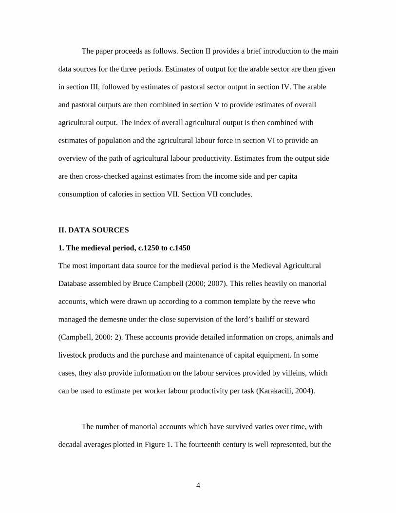
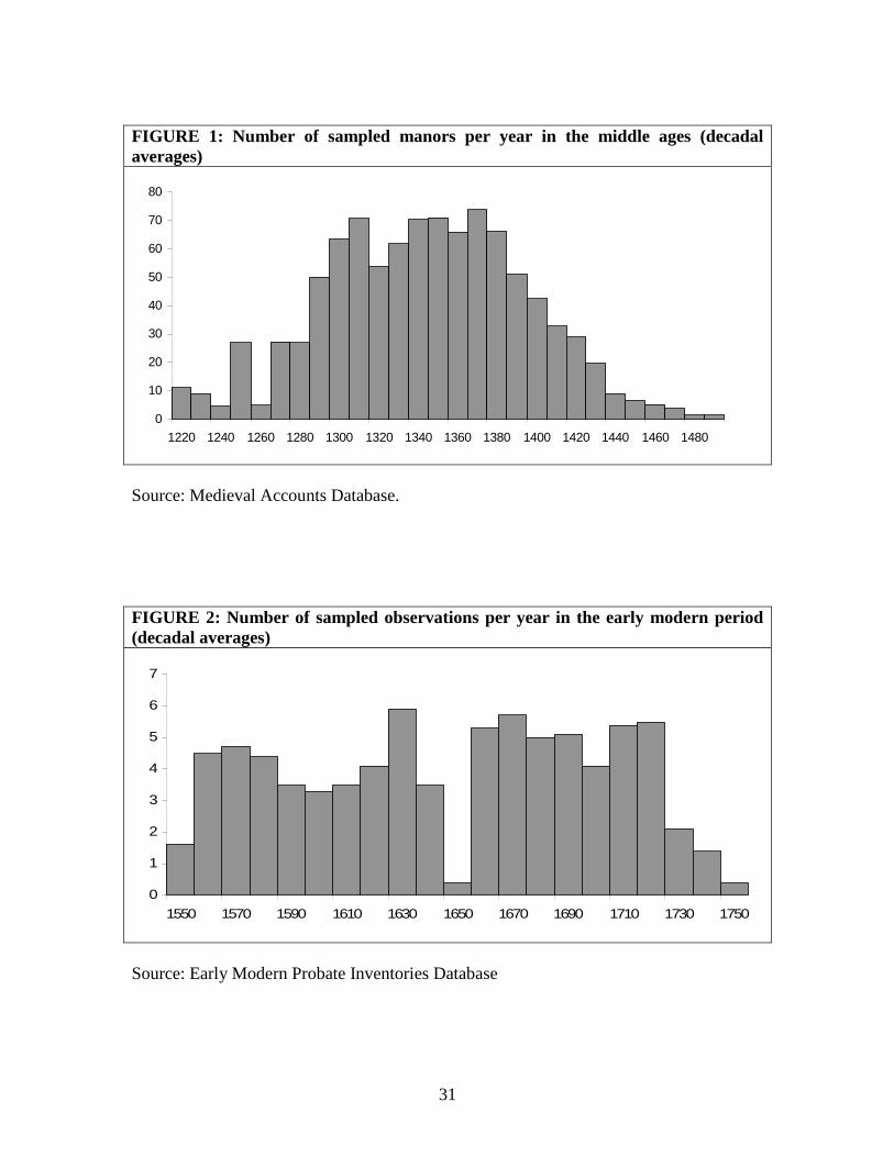
The number of manorial accounts which have survived varies over time, with

decadal averages plotted in Figure 1. The fourteenth century is well represented, but the

5

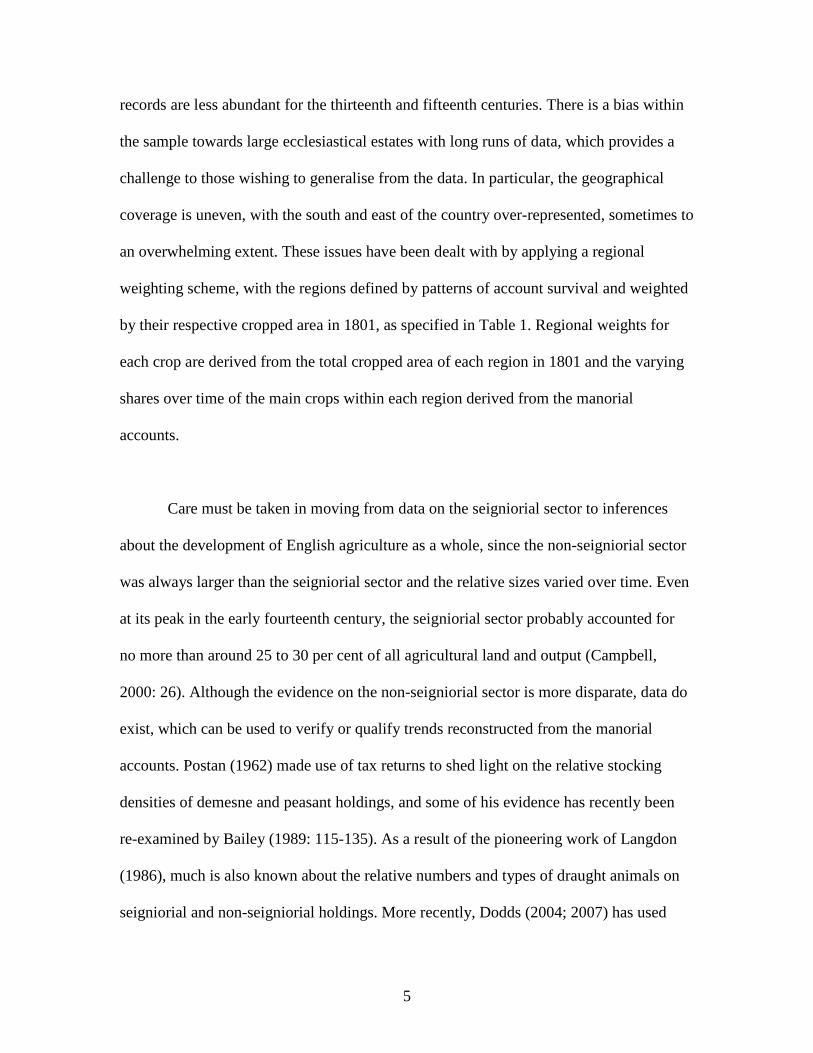
records are less abundant for the thirteenth and fifteenth centuries. There is a bias within

the sample towards large ecclesiastical estates with long runs of data, which provides a

challenge to those wishing to generalise from the data. In particular, the geographical

coverage is uneven, with the south and east of the country over-represented, sometimes to

an overwhelming extent. These issues have been dealt with by applying a regional

weighting scheme, with the regions defined by patterns of account survival and weighted

by their respective cropped area in 1801, as specified in Table 1. Regional weights for

each crop are derived from the total cropped area of each region in 1801 and the varying

shares over time of the main crops within each region derived from the manorial

accounts.

Care must be taken in moving from data on the seigniorial sector to inferences

about the development of English agriculture as a whole, since the non-seigniorial sector

was always larger than the seigniorial sector and the relative sizes varied over time. Even

at its peak in the early fourteenth century, the seigniorial sector probably accounted for

no more than around 25 to 30 per cent of all agricultural land and output (Campbell,

2000: 26). Although the evidence on the non-seigniorial sector is more disparate, data do

exist, which can be used to verify or qualify trends reconstructed from the manorial

accounts. Postan (1962) made use of tax returns to shed light on the relative stocking

densities of demesne and peasant holdings, and some of his evidence has recently been

re-examined by Bailey (1989: 115-135). As a result of the pioneering work of Langdon

(1986), much is also known about the relative numbers and types of draught animals on

seigniorial and non-seigniorial holdings. More recently, Dodds (2004; 2007) has used

6

tithe records to shed light on annual variations in grain output, and a few tithe series

contain wool output. Campbell (2007) shows that there is a close correlation between

year-on-year fluctuations in crop yields derived from manorial accounts and annual

changes in tithe receipts.

Seigniorial and non-seigniorial producers faced a common environment and

commercial opportunities and a common technology, while there was much overlap

between their labour forces. Hence, where peasants led, lords were likely to follow and

vice versa (Campbell, 2000: 1). However, there were important differences in scale of

production, capital resources, consumption priorities, vulnerabilities to risks and hazards

and methods of decision making. Between the mid-thirteenth century and the mid-

fourteenth century, factor costs and property rights encouraged lords to manage their

demesnes directly and concentrate on arable production. Following the Black Death,

however, lords found it increasingly difficult to obtain customary labour, and

increasingly expensive to hire wage labour, following a substantial increase in wage

rates. Those lords who continued to farm directly switched away from labour intensive

arable production to mixed husbandry and pastoral production, leaving arable production

to peasants who could rely mainly on family labour and were unburdened by

administrative overheads. Increasingly, lords thus found it more profitable to lease out

their demesnes, and by the mid-fifteenth century, very few demesnes were directly

managed.

7

In the calculations that follow, trends in grain yields per unit area on the demesne

lands are taken as representative of arable farming as a whole. Patterns of demesne

cropping are also treated as broadly representative of arable husbandry in general. The

total amount of land under crop at its maximum is based upon the equivalent area in

1801, with allowance made for net changes in the interim arising from reclamation and

enclosure on the one hand and the conversion of tillage to pasture on the other.

Deviations from that maximum pre and post c.1300 are determined from trends in

demesne sown areas and aggregate tithe receipts. Estimates of the amounts of grain

consumed in the production process as seed and fodder are based upon relevant

information contained in the manorial accounts. With these four items of information —

crop yields, crop proportions, crop areas, and grain used as seed and fodder — it is a

comparatively straightforward exercise to estimate the total net output of each crop each

year. Self evidently, in the absence of significant grain imports the total net output of

grain had to be sufficient, when converted into bread, pottage, and ale, to satisfy the

nation’s food and drink requirements at a time when grain probably supplied on average

at least 75 per cent of all kilocalories consumed.

Deriving equivalent estimates for livestock is more problematic, since it is less

likely that stocking densities and stock proportions within the seigniorial sector are

broadly representative of all classes of producer. On the contrary, there is good evidence

to suggest that significant differences existed between the relative numbers and types of

animals stocked on large demesne and small peasant holdings, Moreover, these

differences probably widened following the Black Death as contrasting factor costs lent

8

greater momentum to the shift away from arable farming within the demesne sector. This

applies in particular to sheep, where trends in the seigniorial and non-seigniorial sectors

were very different. The one certain fact about sheep is the numbers needed to produce

the fleeces exported as wool and woollen cloth recorded from 1275 in the annual customs

accounts. How many additional sheep were engaged in supplying wool to the domestic

market is then a matter of estimation. For these reasons, estimates for the pastoral sector

are subject to greater uncertainty than those for the arable and are likely to undergo

significant revision as further information becomes available.

2. The early modern period, c.1550 to c.1750

Between the mid-sixteenth and the mid-eighteenth centuries, we rely on probate

inventories for our basic information on agriculture. Probate inventories recorded the area

of major crops and the stock of farm animals, as well as their values at the time of a

farmer’s death. From this information, it is possible to derive the key magnitudes that

were recorded directly in the medieval manorial accounts: grain yields and animal

stocking densities. Probate inventories containing this information first became available

in the 1550s, but declined from the early eighteenth century as church courts no longer

kept the inventories once probate had been granted. The number of inventories in the

sample is plotted in decadal average form in Figure 2, for comparison with the manorial

accounts database. Perhaps surprisingly, the early modern period is less well served than

the medieval period for surviving records on the agricultural sector.

9

To derive grain yields from probate inventories, the starting point in Overton

(1979) is the identity v=py, where v is the valuation per acre of growing grain recorded in

probate inventories, p is the price per bushel after the harvest and y is the yield in bushels

per acre. The yield is thus obtained from the valuation and the price as:

y = v/p (1)

However, the calculations are more complex in practice because appraisers subtracted

10% of gross output for tithes, and care must also be taken to allow for the costs of

reaping (r), threshing (t) and carting (c), which affected the value that the appraisers

placed on a growing crop. Allen’s (1988) valuation equation, accepted by Overton (1990)

and Glennie (1991) thus becomes:

v = 0.9 (py - ty - c) –r (2)

Rearranging for comparison with equation (1), the yield becomes:

)(9.0

9.0

tp

crvy

(3)

A further complication concern the months used for the crop valuations, since appraisers

often valued crops in early months of the year by listing the costs incurred in bringing the

crop to its current condition, thus resulting in spuriously low yields. Allen (1988)

excludes these observations by setting a minimum yield of 5 bushels per acre, but this has

the disadvantage of also excluding genuinely bad harvests. We follow Overton (1979:

369) in restricting our attention to valuations in the months of June to August.

As in the medieval period, care must be taken in generalising to the national level

from individual farm observations. Although inventories have survived for a wide range

of farm sizes, the very largest and the very smallest farms are under-represented (Overton

10

and Campbell, 1992: 380). But perhaps most importantly, the geographical coverage of

the probate inventories sample is heavily skewed to the south of the country (Cornwall,

Durham, Hertfordshire, Kent, Lincolnshire, Norfolk, Suffolk and Worcestershire). These

issues have been dealt with in a similar fashion to those of the medieval period, by

applying a regional weighting scheme based on the total cropped area of each region in

1801 and the varying shares over time of the main crops within each region. Regional

shares of sown acreage are taken from Turner (1981), based on the 1801 crop returns and

the Early Modern Probate Inventories Database for other years.

In contrast to the medieval period, there are no continuous runs of data on

individual farms, but only one-off observations determined by the death of farmers. In

estimating grain yields and stocking densities, this is dealt with by assuming comparable

series in similar agricultural regions, hence introducing a time series aspect, as suggested

by Clark (2004). The animal sector was calculated on the basis of stocking densities

(animals per hundred sown acres) that can vary from 0 (no animals on a farm) to a very

high figure. A modification of Clark’s (2004) method was therefore necessary, using a

tobit regression in order to capture farms with a stocking density of 0. Because the

variance of farm size in the early modern period is considerably higher than that of the

domain sector in the medieval period, which has a strong impact on the stocking

densities, we introduced dummy variables to capture farm size.

It will be apparent that there remains a statistical dark age for grain yields and

animal stocking densities between the decline of the manorial sector in the late fifteenth

11

century and the systematic appearance of probate inventories in the mid-sixteenth

century. We propose to deal with this period by using information on prices and income

to estimate the demand for agricultural goods, as suggested by Crafts (1976; 1985) and

further explored for the modern period by Allen (1994; 2000). This can be done both by

projecting forwards on the basis of a medieval demand system and by projecting

backwards on the basis of an early modern demand system.

3. The modern period, c.1700 to c.1850

Perhaps surprisingly, the least well documented period is that nearest the present.

However, an important step forward has recently been taken with the collection by

Turner, Beckett and Afton (2001) of a sample of farm accounts from the 1720s to the

outbreak of World War I. These farm accounts are much less standardised than the

medieval manorial accounts, but they do provide crucial data on the amount of land in

use and crops sown and harvested, which allows the derivation of grain yields. Perhaps

disappointingly, data on numbers of farm animals were not systematically collected,

although there are some data on sales of animals.

As with the medieval and early modern samples, the modern sample of farm

records is uneven in both temporal and spatial coverage. Figure 3 sets out the

chronological distribution of the sampled farm records. Although the evidence is

relatively thin for the first half of the eighteenth century, this period can be bolstered by

the surviving probate inventories. The sample is stronger for the first half of the

nineteenth century. The spatial distribution of farm records is more even than for the

12

medieval and early modern periods, with the north and west of the country almost as well

represented as the south and east (Turner, Beckett and Afton, 2001: 64). Nevertheless, it

is still important to apply a regional weighting scheme, as for the earlier periods. There is,

of course, a danger that the surviving records are biased towards the better run farms,

since there was no requirement to keep farm accounts. However, the farm accounts data

are checked against the probate inventory data in the first half of the eighteenth century

and against the official output data from the late nineteenth century to gauge yield levels.

Given the lack of data on animal stocking densities in the farm accounts, animal

numbers have been gleaned from estimates by agricultural historians for benchmark

years, and interpolated using data on annual sales at Smithfield Market from Mitchell

(1988: 708). Pastoral sector outputs have also been checked against estimates using the

demand approach outlined in the previous section, the results of which are discussed in

Broadberry and van Leeuwen (2008).

III. ARABLE OUTPUT AND ITS COMPONENTS

1. Land use

The starting point for any estimate of the output of the arable sector is the total area under

crop, which is set out in Table 2A. For most benchmark years, the data are taken from

Overton and Campbell (1996). Firm estimates of land use only became available in the

agricultural returns for 1871, which therefore provides the starting point for the series.

For 1830, the figures come from the tithe files and for 1800, 1750 and 1700 from

estimates by contemporaries (Holderness, 1989). The estimates for 1600 have been

13

inferred by extrapolating backwards from these later figures. For the medieval period, the

starting point is the estimate for 1300, when the population attained its medieval peak.

Contrary to the claims of Clark (2007a: 124), it is unlikely that the sown area in 1300

could have been above the 1800 acreage. Estimates for 1420, 1380, and 1250 are

obtained by extrapolation from 1300 on the basis of trends in the cropped acreage on

demesnes and tithe data (Campbell et al., 1996). Total arable land in use fell across the

Black Death as population declined sharply, and increased continuously from a low point

in the fifteenth century.

Having obtained estimates of the overall arable acreage in use, the next step is to

allocate it between fallow and the major crops sown. This information is taken from the

three datasets described in section II. The amount of fallow land is first subtracted in

Table 2A, and the resulting sown area is allocated between the major crops in Table 2B.

The proportion in fallow was typically around one third in the medieval period, falling

below a quarter in the early modern period and to just 3.5 per cent by 1871. The regional

distribution of the crop totals contained in Table 2B is given in Table 3 for the seven

regional groupings adopted for structuring and weighting the available agricultural data.

These weightings are crucial to the process of aggregating to a national level from data

that are intrinsically local and of uneven geographical coverage. Each region’s share of

the national sown acreage is taken from the 1801 crop returns. Within each region, the

breakdown of crops is based upon information provided by the medieval and early

modern databases, and for later periods by Holderness (1989) and Overton (1996).

Amongst the principal winter-sown crops, wheat remained important throughout the

14

period, but rye and maslin (a mixture of wheat and rye) declined sharply during the early

modern period. Amongst the spring-sown crops, barley and dredge (a mixture of barley

and oats) remained important throughout the period, but oats declined in relative

importance. The biggest increase in the use of arable land was in potatoes and other

crops, particularly after 1700. The most rapid increase in other crops was in clover and

root crops such as turnips, parsnips and rape. Since clover fixes more nitrogen, its

growing use led to a substantial improvement in soil quality (Overton, 1996: 110). The

increasing share of turnips in sown acreage provided a more solid food base for the

animal stock in the winter and increased opportunities for manuring the land, since the

animals were allowed to graze on the land (Overton, 1996: 99-101).

2. Grain yields

To calculate the output from the estimated areas sown with each crop requires

information on grain yields per unit area, net of seed sown. For the medieval and modern

periods, direct information on the seed sown, areas sown and quantities of grain

harvested and threshed can be obtained from manorial accounts and farm records. For the

early modern period, grain yields have to be estimated indirectly from probate inventories

following the approach set out in Section II.2, based on the work of Overton (1979;

1990), Allen (1988) and Glennie (1991).

Generating aggregate trends in grain yields from the information obtained from

individual manors, probate inventories and farm accounts is not straightforward. The first

problem concerns the regional weightings. Given the extent of variation in yields across

15

individual units of observation, it is necessary to ensure an appropriate regional coverage

and to allow for the changing spatial composition of the sample. The available dataset has

therefore been subdivided into the seven regional groupings identified in Table 1.

Separate chronologies reconstructed for each of these regions have then been combined

into a single weighted master chronology for the country as a whole. The early modern

probate inventory data are necessarily one-off observations rather than time series, and

the time series are typically rather short and discontinuous in the modern farm accounts

and medieval manorial accounts databases. The chronologies are therefore derived using

regression analysis with dummy variables for each farm and for each year, as suggested

by Clark (2004). Since the dispersion of grain yields across farms is very high, it is

important to use a log-linear specification, otherwise a small percentage drop in output on

a high-yielding farm can outweigh a large percentage increase on a low-yielding farm.

Adjustment has also been made for tithes deducted at source and assumed to have been

10 per cent of the gross harvested crop.

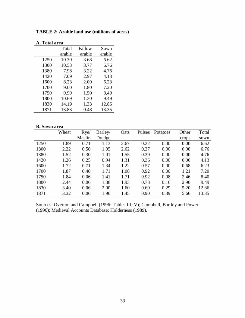
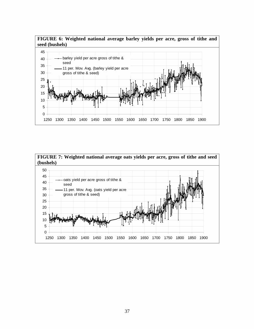
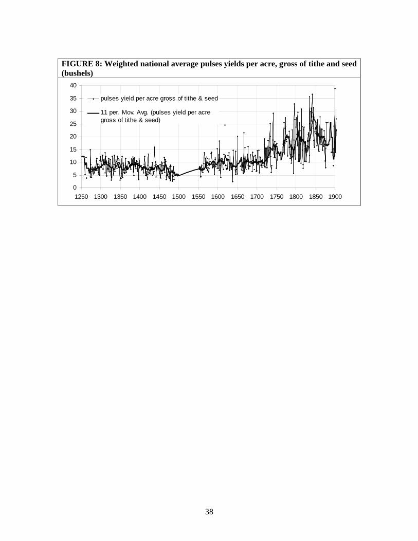
Annual variations and long-term trends in yields obtained in this way for wheat,

barley, rye, oats and pulses are shown in Figures 4 to 8. In addition, summary

information on gross yields per acre, seeding rates and net yields is presented in Table 4

as fifty-year averages, to abstract form short run fluctuations, which were very

pronounced. As will be observed, the crops differed in their overall levels of yield, with

rye delivering higher yields per acre than wheat in the medieval and early modern

periods, with barley also delivering higher yields than oats in the medieval and early

modern periods, and with pulses producing the lowest yields of all crops throughout the

16

period. Yields also varied a great deal from year to year and over longer periods of time.

Although there is an unfortunate gap between the late fifteenth century and the mid-

sixteenth century, the three data sets appear to tell a consistent story, with yields

declining during the late medieval period from around 1300, picking up again during the

early modern period from the mid-sixteenth century, and growing more rapidly during

the modern period from the early eighteenth century. Eleven year moving averages have

been shown as well as the annual data, to help to abstract from the high degree of short

run volatility.

3. Consumption by working animals

In addition to making allowance for grain used as seed, calculation of the net output of

the arable sector must take account of consumption of oats and pulses by animals

working on the farm. For pulses it is assumed, following Allen (2005), that half of output

was consumed by working farm animals and others, mainly swine, being fattened for

meat. Oats consumed as fodder has been derived by estimating the number of working

animals and consumption per animal.

For the medieval and early modern periods, respectively, estimates of the number

of working animals per 100 sown aces can be obtained from the medieval accounts and

probate inventory databases. For the early modern period, these stocking densities are

assumed to apply to the whole agricultural sector and hence are simply multiplied with

the sown acreage to produce estimates of the numbers of working animals. However, for

the medieval period, the demesne stocking densities have been converted into the

17

numbers of horses and oxen on all lands using Wrigley’s (2006: 449) assumption that the

stocking density of animals on non-seigniorial holdings was three-quarters that on the

demesnes. In making these estimates, allowance has been made for both the declining

share of demesne acreage and the lesser quantities of fodder consumed by immature

animals. For the modern period, direct estimates of animal numbers are taken from John

(1989) and Allen (2005), since data on stocking densities are unavailable.

As with the crop yields, a regional weighting scheme is needed to derive the

stocking densities for the country as a whole from the observations on individual

demesnes and farms. The regional groupings chosen are different from those used for

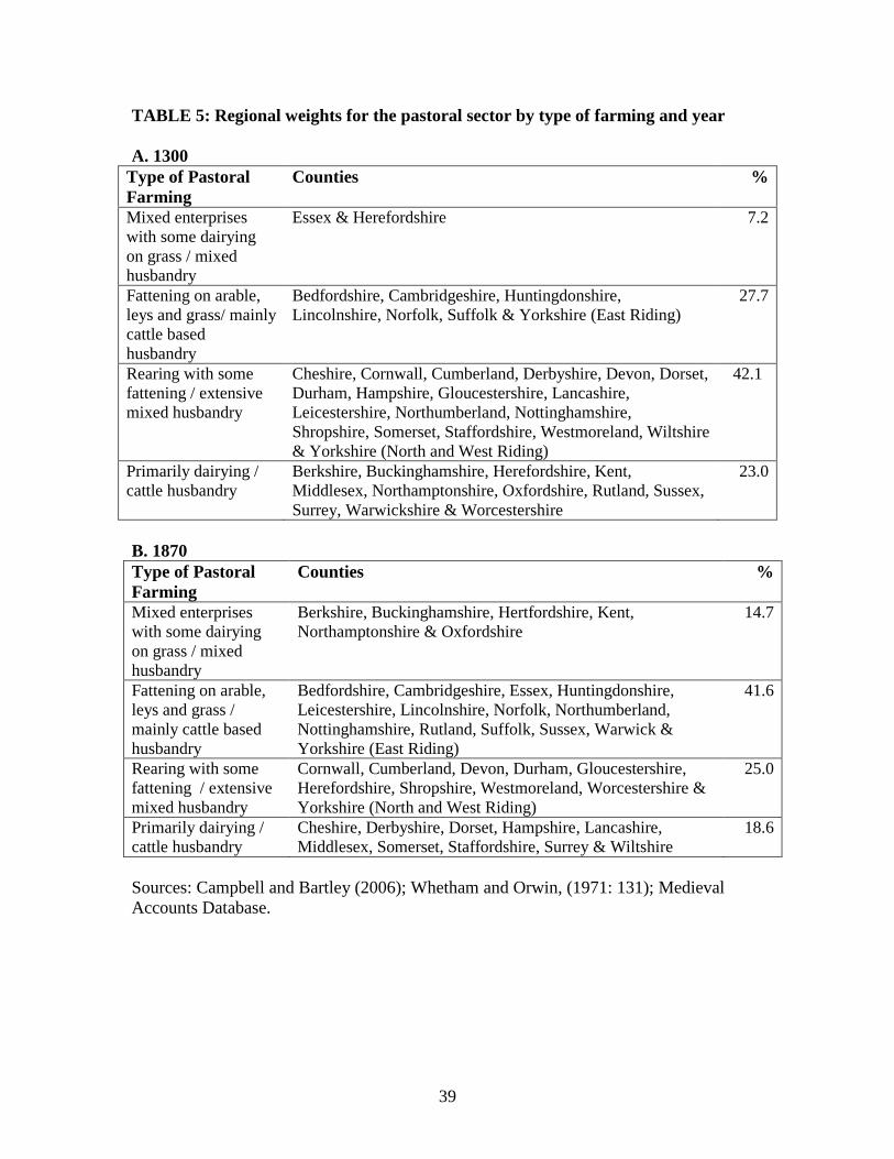
arable farming, reflecting the four main types of pastoral farming. Table 5 sets out the

regional weights for the pastoral sector in 1300 and 1870. It is noteworthy that although

by 1870 dairying had spread to counties where it had been scarce in 1300, the core

activities of farms, especially in the north-western counties, had shifted towards the

fattening of cattle.

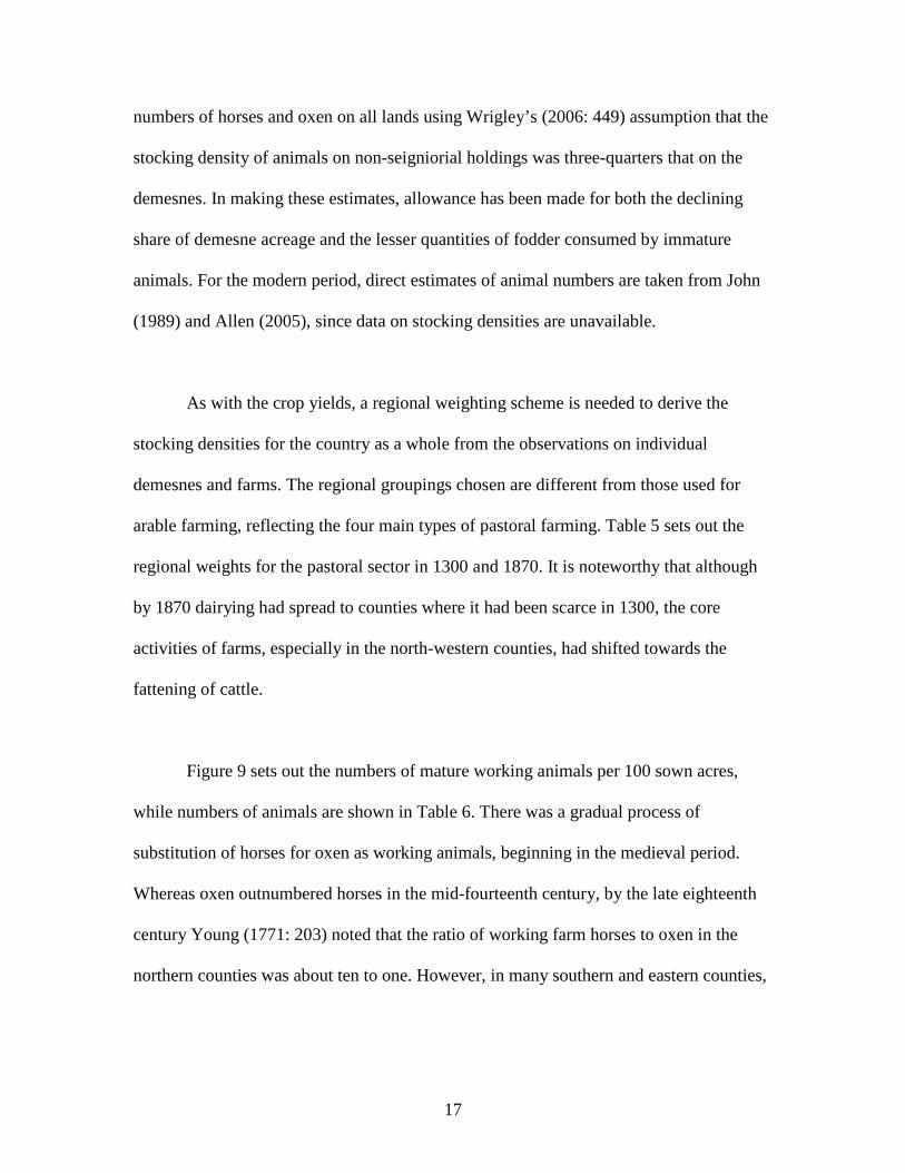
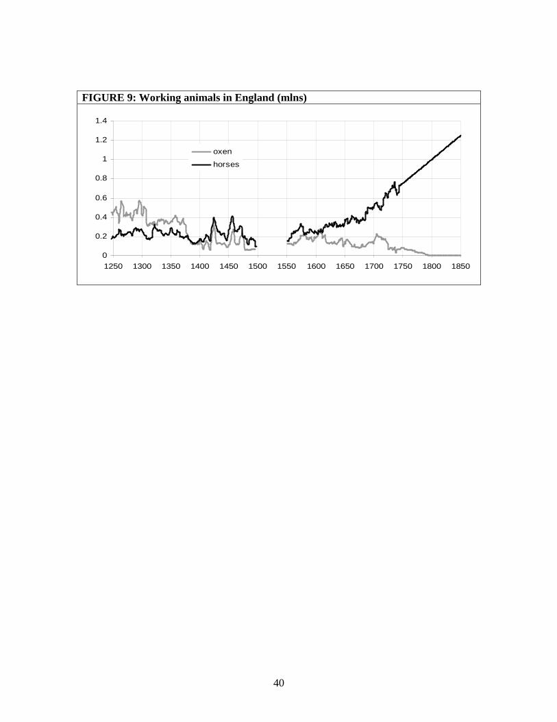
Figure 9 sets out the numbers of mature working animals per 100 sown acres,

while numbers of animals are shown in Table 6. There was a gradual process of

substitution of horses for oxen as working animals, beginning in the medieval period.

Whereas oxen outnumbered horses in the mid-fourteenth century, by the late eighteenth

century Young (1771: 203) noted that the ratio of working farm horses to oxen in the

northern counties was about ten to one. However, in many southern and eastern counties,

18

the ox had already been replaced by the horse several decades earlier (Perkins, 1975: 4).

The use of oxen had more or less died out by the nineteenth century.

Overton and Campbell (1996) estimate the total consumption of oats by animals

in 1800 as 70 percent of total net output. Assuming non-farm horses ate slightly more

oats than farm horses, dividing the share of output consumed by animals by the number

of animals results in an average consumption of 26 bushel per mature horse, since the

number of oxen was set to zero from 1800 onwards. This is consistent with the estimate

of Vancouver (1808) that a working horse consumed half a peck (one eighth of a bushel)

during winter and periods of intensive work, which would amount to roughly 200 days a

year. For both oxen and horses, immature animals are assumed to consume half the

amount of mature animals (Allen, 2005 and Langdon, 1982; 1986), and the share of

immature animals is assumed to be 35 percent (Wrigley, 2006). For the medieval period,

the proportion of oats consumed by animals is assumed to be 50 per cent in 1600 and at

most 30 per cent in 1300 (Overton and Campbell, 1996; Wrigley, 2006). Allowance is

also made for the lower consumption per animal on non-demesne lands in 1300, as

suggested by Langdon (1982), but with the difference disappearing by 1500 as the

demesne sector effectively disappeared. Consumption of oats per animal in 1300 was 16

bushels for a horse and 2.72 bushels for an ox on demesne lands (or 8 and 1.36 bushels,

respectively, on average across demesne and non-demesne lands).

4. Arable output net of seed and animal consumption

19

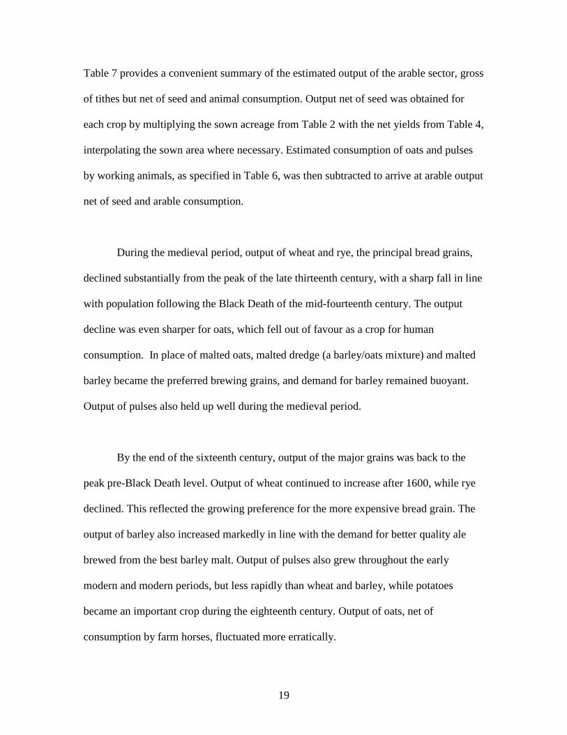
Table 7 provides a convenient summary of the estimated output of the arable sector, gross

of tithes but net of seed and animal consumption. Output net of seed was obtained for

each crop by multiplying the sown acreage from Table 2 with the net yields from Table 4,

interpolating the sown area where necessary. Estimated consumption of oats and pulses

by working animals, as specified in Table 6, was then subtracted to arrive at arable output

net of seed and arable consumption.

During the medieval period, output of wheat and rye, the principal bread grains,

declined substantially from the peak of the late thirteenth century, with a sharp fall in line

with population following the Black Death of the mid-fourteenth century. The output

decline was even sharper for oats, which fell out of favour as a crop for human

consumption. In place of malted oats, malted dredge (a barley/oats mixture) and malted

barley became the preferred brewing grains, and demand for barley remained buoyant.

Output of pulses also held up well during the medieval period.

By the end of the sixteenth century, output of the major grains was back to the

peak pre-Black Death level. Output of wheat continued to increase after 1600, while rye

declined. This reflected the growing preference for the more expensive bread grain. The

output of barley also increased markedly in line with the demand for better quality ale

brewed from the best barley malt. Output of pulses also grew throughout the early

modern and modern periods, but less rapidly than wheat and barley, while potatoes

became an important crop during the eighteenth century. Output of oats, net of

consumption by farm horses, fluctuated more erratically.

20

IV. PASTORAL OUTPUT

1. Numbers of non-working animals

The starting point for deriving the numbers of non-working animals is again the stocking

densities. As with the working animals, particular care must be taken for the medieval

period in moving from the stocking densities on the demesnes to the numbers of animals

in the country as a whole. Conversion of the seigniorial stocking densities into

corresponding national densities and numbers of animals is based on four key

assumptions. First, following Allen (2005), it has been assumed that due to their high unit

capital value, the density of cattle was one-third lower on the non-demesne lands.

Second, again following Allen (2005), mature cattle have been divided into milk and beef

animals in the ratio 53 to 47 percent. Third, swine, a quintessentially peasant animal, are

assumed to have been stocked at double the density by non-seigniorial producers

(Wrigley, 2006). Fourth, aggregate sheep numbers are assumed to have been stationary

in the long term, in contrast to their dynamic growth in the seigniorial sector. This is

consistent with trends in exports, inferred levels of domestic demand, and the decline in

average fleece weights noted by Stephenson (1988: 380). Total sheep numbers have been

set at 15 million in 1300, in line with the estimate of Wrigley (2006: 448). This was the

number of animals needed to supply the wool export trade as recorded by the customs

accounts (Britnell, 2004: 417) and a domestic consumption equivalent of 1.18 square

yards per head per annum, on the reckoning that domestic production supplied labourers

with 1 square yard of woollen cloth, substantial tenants with 2 square yards and

landowners with 8 square yards, weighting the different social classes according to the

21

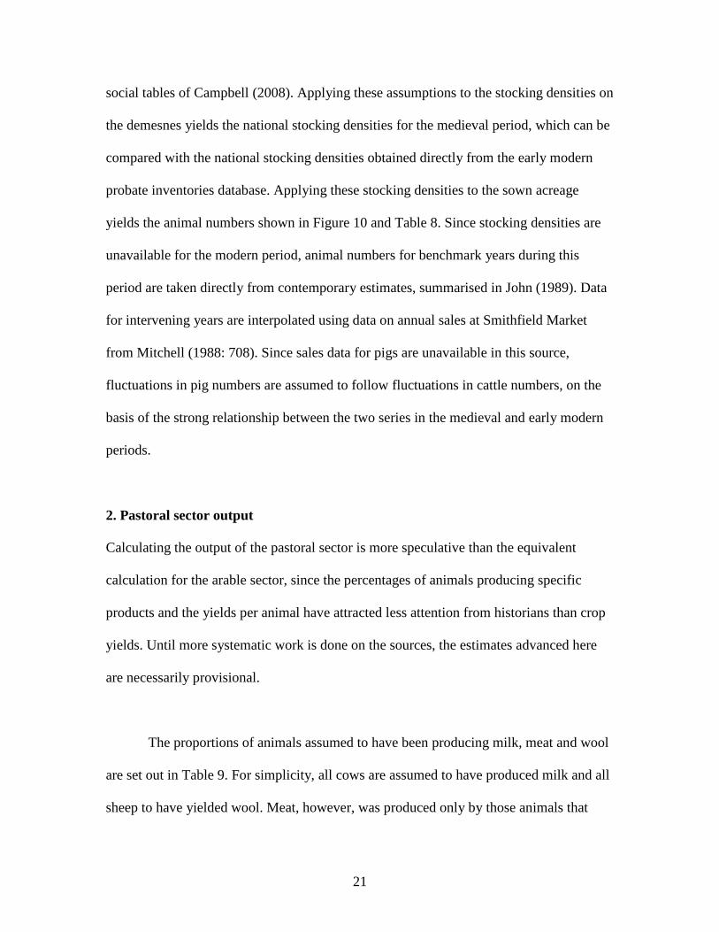
social tables of Campbell (2008). Applying these assumptions to the stocking densities on

the demesnes yields the national stocking densities for the medieval period, which can be

compared with the national stocking densities obtained directly from the early modern

probate inventories database. Applying these stocking densities to the sown acreage

yields the animal numbers shown in Figure 10 and Table 8. Since stocking densities are

unavailable for the modern period, animal numbers for benchmark years during this

period are taken directly from contemporary estimates, summarised in John (1989). Data

for intervening years are interpolated using data on annual sales at Smithfield Market

from Mitchell (1988: 708). Since sales data for pigs are unavailable in this source,

fluctuations in pig numbers are assumed to follow fluctuations in cattle numbers, on the

basis of the strong relationship between the two series in the medieval and early modern

periods.

2. Pastoral sector output

Calculating the output of the pastoral sector is more speculative than the equivalent

calculation for the arable sector, since the percentages of animals producing specific

products and the yields per animal have attracted less attention from historians than crop

yields. Until more systematic work is done on the sources, the estimates advanced here

are necessarily provisional.

The proportions of animals assumed to have been producing milk, meat and wool

are set out in Table 9. For simplicity, all cows are assumed to have produced milk and all

sheep to have yielded wool. Meat, however, was produced only by those animals that

22

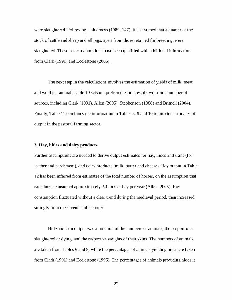
were slaughtered. Following Holderness (1989: 147), it is assumed that a quarter of the

stock of cattle and sheep and all pigs, apart from those retained for breeding, were

slaughtered. These basic assumptions have been qualified with additional information

from Clark (1991) and Ecclestone (2006).

The next step in the calculations involves the estimation of yields of milk, meat

and wool per animal. Table 10 sets out preferred estimates, drawn from a number of

sources, including Clark (1991), Allen (2005), Stephenson (1988) and Britnell (2004).

Finally, Table 11 combines the information in Tables 8, 9 and 10 to provide estimates of

output in the pastoral farming sector.

3. Hay, hides and dairy products

Further assumptions are needed to derive output estimates for hay, hides and skins (for

leather and parchment), and dairy products (milk, butter and cheese). Hay output in Table

12 has been inferred from estimates of the total number of horses, on the assumption that

each horse consumed approximately 2.4 tons of hay per year (Allen, 2005). Hay

consumption fluctuated without a clear trend during the medieval period, then increased

strongly from the seventeenth century.

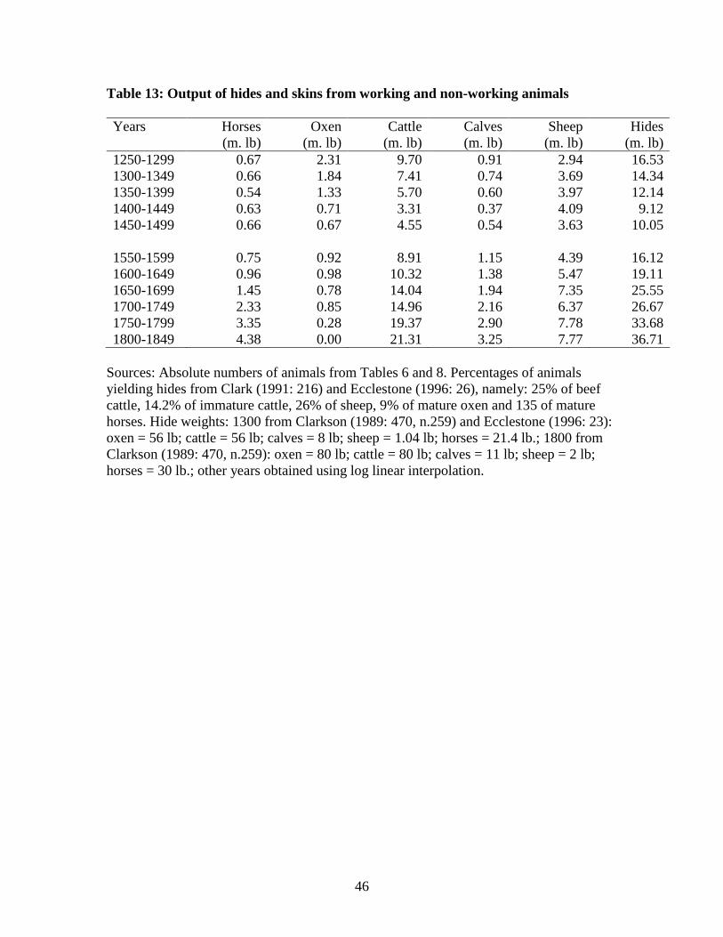
Hide and skin output was a function of the numbers of animals, the proportions

slaughtered or dying, and the respective weights of their skins. The numbers of animals

are taken from Tables 6 and 8, while the percentages of animals yielding hides are taken

from Clark (1991) and Ecclestone (1996). The percentages of animals providing hides is

23

assumed to be stable throughout the period, but hide weights changed over time with the

size of animals. Hide weights are established for benchmark years of 1300 and 1800 and

interpolated log-linearly. The hide weights for 1800 are based on the estimates of

Clarkson (1989), while those for 1300 rely also on the work of Ecclestone (1996). Total

output of hides and skins declined during the medieval period, although the supply of

skins from sheep remained relatively stable while the supply from cattle and oxen fell.

From the sixteenth century there was a clear upward trend in the supply of hides, with

strong growth from cattle as well as sheep. There was also a substantial increase in the

supply of hides from horses, reflecting the growing use of horses both on and off farms.

In the dairy sector, the bulk of the milk output in Table 11 was used on the farm

to produce butter and cheese. The breakdown of the total milk production between butter,

cheese and fresh milk is shown in Table 14. For the medieval period, the cheese to butter

ratio is based on Biddick’s (1989: Appendix 5) study of the estates of Bolton Priory in the

Pennine uplands of northern England. For the modern period, the division between fresh

milk, butter and cheese is taken from Holderness (1989: 169-170), who provides data for

1750, 1800 and 1850. The breakdown for other years is based on log-linear interpolation.

The output of the dairy sector as a whole is constrained to move in line with total milk

output in Table 11, declining during the medieval period but trending upwards strongly

from the sixteenth century. The share of fresh milk in total milk output was stable during

the medieval period, but increased from the late seventeenth century. The ratio of butter

to cheese also increased during the modern period, with butter becoming more important

over time. The high share of cheese in dairy output during the medieval period was a

24

result of the fact that butter spoils quickly, so that it was not a practical way of preserving

the nutrients of milk (Dyer, 1988). However, this changed from the early eighteenth

century as a result of improvements in hygiene and the introduction of the barrel churn,

mounted on a wooden stand so that it could revolve, and fitted with handles to turn it

(Fussell, 1963: 217).

V. TOTAL AGRICULTURAL OUTPUT

Multiplying the output volumes by their prices yields the total value of net output. The

price data are taken largely from Clark (2004), who synthesises the published data of

Beveridge (1939), Thorold Rogers (1866-1902: volumes 1-30) and the multi-volume

Agrarian History of England and Wales, as well as integrating new archival material,

principally from the unpublished papers of William Beveridge and David Farmer. To

this, have been added the prices of hides from Thorold Rogers (1866-1902: volumes 1-

30) and of rye from Farmer (1988; 1991). Where there are large gaps in the price data for

individual products, regression analysis has been used to interpolate the missing values.

Output can be valued in both current prices and in constant 1700 prices.

Figure 11 plots arable, pastoral and total agricultural output in constant prices on a

logarithmic scale, while Table 15 summarises the same information in growth rate form,

using 5-year averages. During the medieval period, arable output exhibited a downward

trend, while pastoral output showed long run stability. Agriculture as a whole thus

showed a modest decline in output. As a result of these trends, the pastoral sector

increased its share of output in constant price terms. The increasing share of the pastoral

25

sector during the medieval period can also be seen in current price terms in Figure 12 and

Table 16. The current price share is affected by the trend in the relative price of pastoral

to arable products, as well as the real growth rates of the two sectors, but during the

medieval period there was no long run shift in the relative price ratio (Figure 13). From

the mid-sixteenth century, arable and pastoral output grew at similar rates in real terms.

This resulted in a declining share of the pastoral sector in current price output because of

a fall in the relative price of pastoral products.

VI. AGRICULTURAL LABOUR PRODUCTIVITY

To see what happened to labour productivity, it is necessary to provide estimates of the

total population and the share working in agriculture. Although the population of England

has been reconstructed firmly by Wrigley and Schofield (1989) and Wrigley et al. (1997)

for the period since the compulsory registration of births, marriages and deaths, estimates

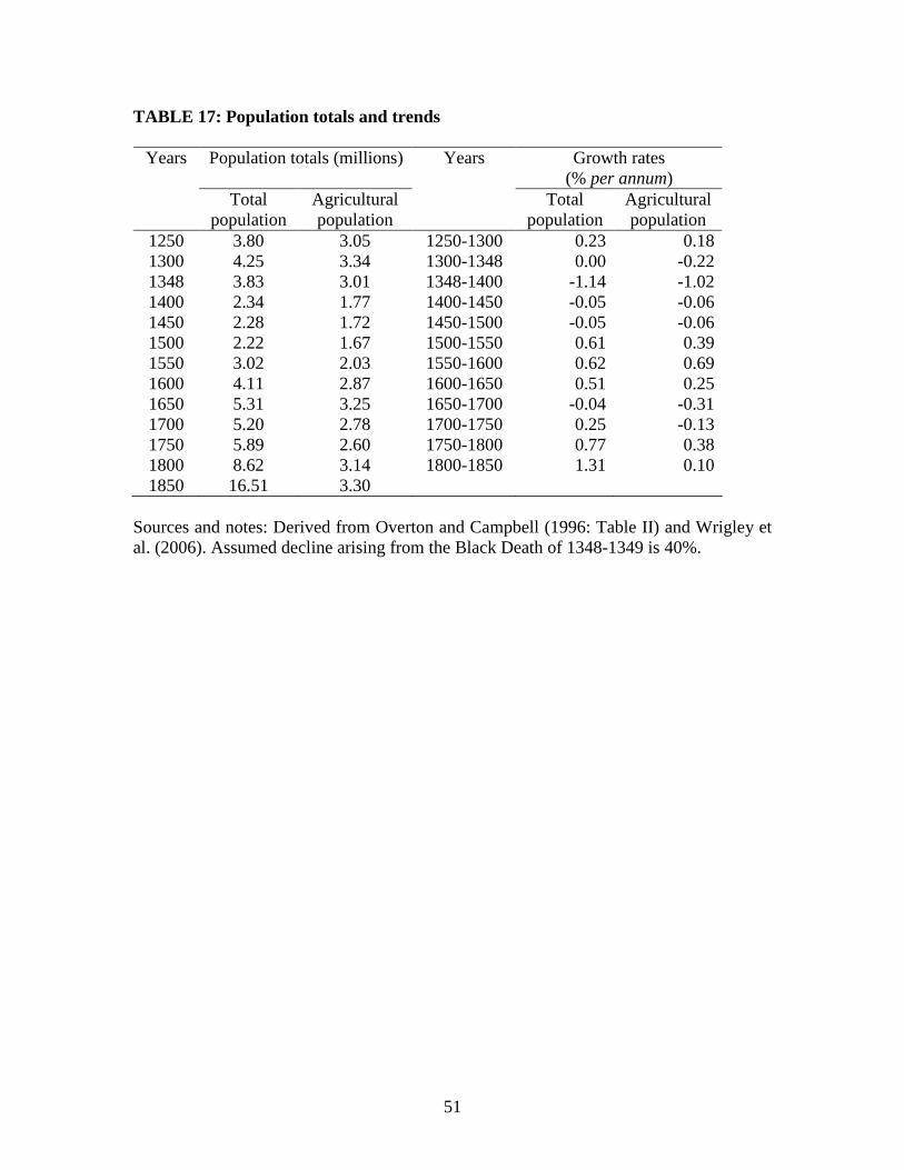
before 1541 are more speculative. The biggest controversy concerns the size of the

population before the Black Death, with the 1380 data more firmly grounded in the poll

tax returns. In Table 17, the population in 1300 is set at 4.25 million, following Overton

and Campbell (1996: Table II). This lies well below the 6 million suggested by Hatcher

(1977) and Smith (1991), but is better in accordance with the consumption data (see

section VII). Additional observations have been added between 1300 and 1380 by

interpolation using assumptions derived from the literature. This involves the assumption

of a slow rate of decline in the population, punctuated by the dramatic decline of the

Black Death years, 1348-51, and a number of smaller crises. The agricultural population

26

is obtained by subtracting estimates of the urban and rural non-agricultural population

from Overton and Campbell (1996: Table II).

Combining the agricultural output series with the agricultural population data

produces our estimates of agricultural output per labourer in Figure 14. Table 18 presents

the same material in growth rate form. The first main finding is that agricultural labour

productivity increased sharply in the immediate aftermath of the Black Death and

remained at this higher level for the rest of the medieval period, albeit with substantial

fluctuations. The second main finding is that there was a further step-up in agricultural

labour productivity between the mid-fifteenth and mid-sixteenth centuries, with labour

productivity remaining at this higher level until the early eighteenth century, but again

with substantial fluctuations. Contrary to the long run stagnationist view of writers such

as Phelps Brown and Hopkins (1981) and Clark (2007a), then, the English economy was

characterised by trend labour productivity growth through the medieval and early modern

periods, averaging out at nearly 0.2 per cent per annum between 1250 and 1700. England

on the eve of the Industrial Revolution was therefore a much richer and more developed

economy than pre-Black Death England. A third main finding is that the improvement in

labour productivity became a much more continuous process from the early eighteenth

century. Fourth, the rate of labour productivity growth slowed down substantially during

the second half of the eighteenth century before strong growth resumed during the first

half of the nineteenth century.

27

It should be noted that the increase in output per worker across the Black Death

resulted largely from an increase in land per worker rather than an increase in output per

unit of land, which is shown here in Figure 14. Although there is some evidence of a

small increase in output per acre between the medieval and early modern periods, the

main source of the rising output were worker was again an increase in land per worker as

the number of people working in agriculture continued to decline until the early sixteenth

century. The more continuous labour productivity growth from the early eighteenth

century was accompanied by strongly rising output per unit of land.

VII. CROSS-CHECKING THE OUTPUT ESTIMATES

1. Income and output based measures

Figure 16 charts the indexed daily real wage of an unskilled farm labourer between 1250

and 1850. In contrast to the upward trend of agricultural output per worker, daily real

wages in agriculture stagnated over the long run. Putting the two series together in Figure

17 inevitably raises the issue of their compatibility. Here, this issue is pursued within the

framework of historical national accounting, where the value of net output should equal

the value of factor payments to labour, land and capital.

Starting on the income side, data on daily wages and the number of days worked

are needed to calculate payments to labour. The agricultural population estimates from

Table 17 are converted into the number of agricultural families in panel A of Table 19 on

the assumption that the average family consisted of two adults and 2.5 children (Allen,

2005). Allen (2005) then calculates the number of days needed to produce the output and

28

divides this by the number of families to arrive at the days worked per family. Allen’s

figure for days worked per family in 1300 has to be increased in order to reconcile it with

the data and results presented here. In contrast, his estimate for 1500 requires substantial

adjustment downwards, for two reasons. First, the estimate of output in the late fifteenth

century presented here on the basis of the medieval accounts database is substantially

lower than that assumed by Allen, who finds that despite a halving of the population,

agricultural output increased between 1300 and 1500. Second, the substantial increase in

days worked per family which Allen requires to achieve that increase in output would be

hard to square with most accounts of the response to the Black Death, which suggest a

decline in labour intensity (Bowden, 1967: 593-594). On the evidence summarised in

Panel A of Table 19, there was a substantial decrease in the number of days worked per

family between 1270 and 1450, consistent with an “indolent revolution” in contrast to the

suggestion of an “industrious revolution” in the early modern period (de Vries, 1994).

The industrious revolution can be seen in the substantial increase in days worked per

family between the sixteenth and nineteenth centuries.

To estimate total rental income requires data on rents and total land in use, set out

in Panel B of Table 17. Rents are obtained from the data of Clark (2001) and Turner et

al., 1997). The total land in use has to include pasture and meadow as well as arable land,

and is taken from Table 2, but multiplied with the ratio of pasture and meadow to arable

land from Allen (2005). Capital costs and tithes and taxes are also taken from Allen

(2005). Adding together wages, rents, capital incomes and tithes and taxes yields the total

incomes in Panel C, which matches reasonably well the value of output.

29

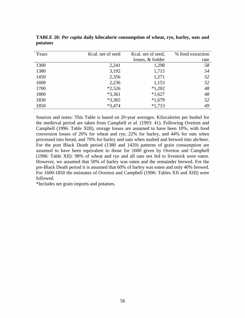
2. Consumption and output

An alternative way of assessing the credibility of the output estimates is to see what they

imply about the level and sufficiency of consumption per head. Converting the output of

the major grains in Table 7 to kilocalories and dividing by the population from Table 17

yields the per capita consumption levels shown in Table 20. Figures in this table are 20-

year averages, to abstract from short run fluctuations. It is reasonable to assume that in a

relatively poor and predominantly agrarian economy such as that of medieval England, at

least three-quarters of daily kilocalorie food requirements were on average supplied by

grain. Livi-Bacci (1991) believes that for a population to have been adequately fed

required an average food intake of 2,000 kilocalories per capita per day. Adult males

labouring on the land would have required about twice this. Net grain output in

agriculture when processed into pottage, bread and ale, thus needed to be able to deliver

at least 1,500 kilocalories per person per day to meet the basic subsistence needs of the

population until that population was sufficiently affluent to devote a larger share of its

budget to dairy produce, meat and fish or meet a substantial proportion of its food

requirements from imports.

The estimates suggest that grain output was sufficient to meet society’s needs

after the Black Death, but was significantly less so in 1300. The picture of English

society in the half century before the Black Death that emerges from this table is one of

an economy under pressure. Note also that it is hard to see how a population much above

the 4.25 million assumed her could have been sustained, given the grain yields and the

30

levels of land use underpinning the output estimates. Although per capita grain

consumption fell back subsequently, the growing share of the pastoral sector would have

provided a higher proportion of kilocalories in 1450 and 1600. By the eighteenth century,

the increase in population was once more putting pressure on the adequacy of the diet,

but by 1800, per capita consumption of kilocalories from grain production, supplemented

by potatoes and grain imports, was again above sufficiency.

VIII. CONCLUSIONS

This paper has provided the first annual estimates of English agricultural output and

labour productivity during the period 1250-1850. The estimates rest on a detailed

reconstruction of arable and pastoral farming, built up from manorial records during the

medieval period, probate inventories during the early modern period and farm accounts

during the modern period. Agricultural labour productivity increased sharply in the

immediate aftermath of the Black Death and remained at this higher level for the rest of

the medieval period. There was a further increase between the mid-fifteenth and mid-

sixteenth centuries, with labour productivity remaining at this higher level until the early

eighteenth century. These pre-modern increases in labour productivity were achieved

without a substantial increase in output per unit of land. The early eighteenth century saw

the start of a continuous upward trend in both agricultural labour productivity and land

productivity.

31

FIGURE 1: Number of sampled manors per year in the middle ages (decadalaverages)

0

10

20

30

40

50

60

70

80

1220 1240 1260 1280 1300 1320 1340 1360 1380 1400 1420 1440 1460 1480

Source: Medieval Accounts Database.

FIGURE 2: Number of sampled observations per year in the early modern period(decadal averages)

0

1

2

3

4

5

6

7

1550 1570 1590 1610 1630 1650 1670 1690 1710 1730 1750

Source: Early Modern Probate Inventories Database

32

FIGURE 3: Number of sampled observations per year in the modern period(decadal averages)

0

2

4

6

8

10

12

14

16

1720 1730 1740 1750 1760 1770 1780 1790 1800 1810 1820 1830 1840 1850 1860 1870

Source: Modern Farm Accounts Database

TABLE 1: Regional shares of the national sown area in 1801

Region Counties %East Anglia Norfolk and Suffolk: 15.3Eastern counties Bedfordshire, Cambridgeshire, Essex, Hertfordshire,

Huntingdonshire, & Lincolnshire:16.7

Southern counties Berkshire Gloucestershire, Hampshire, Herefordshire,Wiltshire, & Worcestershire:

15.5

Southwest Cornwall, Devon, Dorset, & Somerset: 8.9Southeast Kent, Middlesex, Surrey, & Sussex: 8.5Midlands Buckinghamshire, Leicestershire, Northamptonshire,

Oxfordshire, Rutland, & Warwickshire:9.1

North Cheshire, Cumberland, Derbyshire, Durham, Lancashire,Northumberland, Nottinghamshire, Shropshire, Staffordshire,Westmorland, & Yorkshire:

26.0

Source: Turner (1981: Table 1).

33

TABLE 2: Arable land use (millions of acres)

A. Total areaTotal

arableFallowarable

Sownarable

1250 10.30 3.68 6.621300 10.53 3.77 6.761380 7.98 3.22 4.761420 7.09 2.97 4.131600 8.23 2.00 6.231700 9.00 1.80 7.201750 9.90 1.50 8.401800 10.69 1.20 9.491830 14.19 1.33 12.861871 13.83 0.48 13.35

B. Sown areaWheat Rye/

MaslinBarley/Dredge

Oats Pulses Potatoes Othercrops

Totalsown

1250 1.89 0.71 1.13 2.67 0.22 0.00 0.00 6.621300 2.22 0.50 1.05 2.62 0.37 0.00 0.00 6.761380 1.52 0.30 1.01 1.55 0.39 0.00 0.00 4.761420 1.26 0.25 0.94 1.31 0.36 0.00 0.00 4.131600 1.72 0.71 1.34 1.22 0.57 0.00 0.68 6.231700 1.87 0.40 1.71 1.08 0.92 0.00 1.21 7.201750 1.84 0.06 1.41 1.71 0.92 0.08 2.46 8.401800 2.44 0.06 1.38 1.93 0.78 0.16 2.90 9.491830 3.40 0.06 2.00 1.60 0.60 0.29 5.20 12.861871 3.32 0.06 1.96 1.45 0.90 0.39 5.66 13.35

Sources: Overton and Campbell (1996: Tables III, V); Campbell, Bartley and Power(1996); Medieval Accounts Database; Holderness (1989).

34

TABLE 3: Regional weights for the arable sector by year and crop (%)

A. 1300Wheat Rye Barley Oats Pulses

East Anglia 9.2 25.2 41.3 5.8 32.5Eastern counties 24.2 5.2 1.9 19.3 10.9Southern counties 16.1 18.0 21.8 12.3 13.3Southwest 13.4 2.5 0.5 10.4 4.1Southeast 7.4 7.2 10.8 7.0 21.4Midlands 11.3 7.2 10.4 7.3 6.6North 18.5 34.6 13.3 37.9 11.2England 100.0 100.0 100.0 100.0 100.0

B. 1420Wheat Rye Barley Oats Pulses


C. 1600Wheat Rye Barley Oats Pulses


D. 1830Wheat Rye Barley Oats Pulses

East Anglia 15.8 NA 24.3 3.5 12.7Eastern counties 17.2 NA 17.7 13.6 29.5Southern counties 14.9 NA 16.9 9.8 12.9Southwest 8.3 NA 10.1 9.3 5.5Southeast 9.0 NA 5.6 11.3 10.6Midlands 8.6 NA 10.1 6.9 15.0North 26.1 NA 15.3 45.6 13.8England 100.0 100.0 100.0 100.0

Sources and notes: Regional shares of sown acreage from the 1801 crop returns (Turner, 1981);crop shares within each region for each year derived from the Medieval Accounts Database, theEarly Modern Probate Inventories Database and Overton (1996). The original shares for themedieval and early modern periods were calculated as 50 year averages.

35

TABLE 4:Mean yields per acre gross of tithesA. Yield per acre gross of seed (bushels)

Wheat Rye Barley Oats Pulses1250-1299 11.27 13.73 14.41 10.91 8.931300-1349 10.77 13.31 13.36 10.21 8.771350-1399 9.96 12.00 13.67 11.12 8.431400-1449 8.28 13.01 12.20 9.52 7.711450-1499 8.94 16.75 12.74 8.42 6.57

1550-1599 10.38 11.71 12.40 11.87 10.621600-1649 12.95 18.78 15.16 14.97 11.621650-1699 13.86 16.69 16.48 14.82 11.391700-1749 16.36 17.32 19.38 16.27 13.231750-1799 19.54 20.37 25.38 24.90 17.191800-1849 25.56 22.02 29.70 32.37 20.351850-1899 29.19 28.68 27.08 35.36 18.80B. Seed sown per acre (bushels)


1550-1599 2.50 2.50 4.00 4.00 3.001600-1649 2.50 2.50 4.00 4.00 3.001650-1699 2.50 2.50 4.00 4.00 3.001700-1749 2.57 2.50 4.30 4.00 3.001750-1799 2.27 2.50 3.50 4.00 3.001800-1849 2.41 2.50 3.80 4.00 2.501850-1899 2.50 2.50 3.27 4.00 2.50C. Yield per acre net of seed (bushels)


1550-1599 7.88 9.21 8.40 7.87 7.621600-1649 10.45 16.28 11.16 10.97 8.621650-1699 11.36 14.19 12.48 10.82 8.391700-1749 13.79 14.82 15.08 12.27 10.231750-1799 17.26 17.87 21.88 20.90 14.191800-1849 23.16 19.52 25.90 28.37 17.851850-1899 26.69 26.18 23.82 31.36 16.30

Sources and notes: Gross Yield per acre taken from the Medieval Accounts Database, the Early ModernProbate Inventories Database and the Modern Farm Accounts Database. Seed sown per acre from theMedieval and Modern Databases. Pulses for the modern period and all seeds sown for the early modernperiod are taken from Overton and Campbell (1996), Allen (2005).

36

FIGURE 4: Weighted national average wheat yields per acre, gross of tithe and seed(bushels)

0

5

10

15

20

25

30

35

40

45

1250 1300 1350 1400 1450 1500 1550 1600 1650 1700 1750 1800 1850 1900

wheat yield per acre gross of tithe & seed

11 per. Mov. Avg. (wheat yield per acre gross of tithe & seed)

FIGURE 5: Weighted national average rye yields per acre, gross of tithe and seed(bushels)

0

5

10

15

20

25

30

35

40

45

50

1250 1300 1350 1400 1450 1500 1550 1600 1650 1700 1750 1800 1850 1900

rye yield per acre gross of tithe & seed

11 per. Mov. Avg. (rye yield per acregross of tithe & seed)

37

FIGURE 6: Weighted national average barley yields per acre, gross of tithe andseed (bushels)

0

5

10

15

20

25

30

35

40

45

1250 1300 1350 1400 1450 1500 1550 1600 1650 1700 1750 1800 1850 1900

barley yield per acre gross of tithe &seed

11 per. Mov. Avg. (barley yield per acregross of tithe & seed)

FIGURE 7: Weighted national average oats yields per acre, gross of tithe and seed(bushels)

0

5

10

15

20

25

30

35

40

45

50

1250 1300 1350 1400 1450 1500 1550 1600 1650 1700 1750 1800 1850 1900

oats yield per acre gross of tithe &seed

11 per. Mov. Avg. (oats yield per acregross of tithe & seed)

38

FIGURE 8: Weighted national average pulses yields per acre, gross of tithe and seed(bushels)

0

5

10

15

20

25

30

35

40

1250 1300 1350 1400 1450 1500 1550 1600 1650 1700 1750 1800 1850 1900

pulses yield per acre gross of tithe & seed

11 per. Mov. Avg. (pulses yield per acregross of tithe & seed)

39

TABLE 5: Regional weights for the pastoral sector by type of farming and year

A. 1300Type of PastoralFarming

Counties %

Mixed enterpriseswith some dairyingon grass / mixedhusbandry

Essex & Herefordshire 7.2

Fattening on arable,leys and grass/ mainlycattle basedhusbandry

Bedfordshire, Cambridgeshire, Huntingdonshire,Lincolnshire, Norfolk, Suffolk & Yorkshire (East Riding)

27.7

Rearing with somefattening / extensivemixed husbandry

Cheshire, Cornwall, Cumberland, Derbyshire, Devon, Dorset,Durham, Hampshire, Gloucestershire, Lancashire,Leicestershire, Northumberland, Nottinghamshire,Shropshire, Somerset, Staffordshire, Westmoreland, Wiltshire& Yorkshire (North and West Riding)

42.1

Primarily dairying /cattle husbandry

Berkshire, Buckinghamshire, Herefordshire, Kent,Middlesex, Northamptonshire, Oxfordshire, Rutland, Sussex,Surrey, Warwickshire & Worcestershire

23.0

B. 1870Type of PastoralFarming

Counties %

Mixed enterpriseswith some dairyingon grass / mixedhusbandry

Berkshire, Buckinghamshire, Hertfordshire, Kent,Northamptonshire & Oxfordshire

14.7

Fattening on arable,leys and grass /mainly cattle basedhusbandry

Bedfordshire, Cambridgeshire, Essex, Huntingdonshire,Leicestershire, Lincolnshire, Norfolk, Northumberland,Nottinghamshire, Rutland, Suffolk, Sussex, Warwick &Yorkshire (East Riding)

41.6

Rearing with somefattening / extensivemixed husbandry

Cornwall, Cumberland, Devon, Durham, Gloucestershire,Herefordshire, Shropshire, Westmoreland, Worcestershire &Yorkshire (North and West Riding)

25.0

Primarily dairying /cattle husbandry

Cheshire, Derbyshire, Dorset, Hampshire, Lancashire,Middlesex, Somerset, Staffordshire, Surrey & Wiltshire

18.6

Sources: Campbell and Bartley (2006); Whetham and Orwin, (1971: 131); MedievalAccounts Database.

40

FIGURE 9: Working animals in England (mlns)

0

0.2

0.4

0.6

0.8

1

1.2

1.4

1250 1300 1350 1400 1450 1500 1550 1600 1650 1700 1750 1800 1850

oxen

horses

41

TABLE 6: Consumption of oats and pulses by working animals

A. Number of working animals (millions)Horses Oxen Livestock

Units* per100 Acres

Oxen per 100Horses

1250-1299 0.24 0.46 10.63 189.231300-1349 0.24 0.37 10.38 154.971350-1399 0.19 0.26 9.68 136.191400-1449 0.23 0.14 8.50 62.081450-1499 0.23 0.14 8.01 60.10

1550-1599 0.25 0.17 7.73 68.831600-1649 0.30 0.17 8.10 56.031650-1699 0.40 0.11 8.47 28.321700-1749 0.63 0.13 12.11 19.971750-1799 0.87 0.04 13.20 4.631800-1849 1.12 0.00 13.50 0.00

B. Total farm-animal consumption (million bushels)Oats Pulses

1250-1299 2.79 0.861300-1349 2.80 1.151350-1399 2.51 1.121400-1449 2.89 1.001450-1499 3.53 0.91

1550-1599 4.45 1.691600-1649 5.47 1.971650-1699 7.56 2.421700-1749 12.32 2.581750-1799 17.94 3.141800-1849 23.63 3.28

Sources and Notes: Derived from Medieval Accounts Database; Early Modern ProbateInventories Database; Allen (2005); John (1989 Tales III.1 and III.2). Livestock unitscompare different animals on the basis of relative feed requirements. Livestock Ratiosfrom Campbell (2000: 104-107): (Horses x 1) + (Oxen x 1.2).

42

TABLE 7: Arable output net of seed and animal consumption (million bushels)

Wheat Rye Barley Oats Pulses Potatoes1250-1299 17.83 6.66 11.62 16.58 0.86 NA1300-1349 16.37 4.45 9.77 11.91 1.15 NA1350-1399 11.60 2.89 9.78 9.54 1.12 NA1400-1449 7.68 2.87 8.15 5.84 1.00 NA1450-1499 8.95 5.82 7.96 4.18 0.91 NA

1550-1599 12.93 5.31 10.73 5.03 2.42 NA1600-1649 18.37 7.26 16.13 7.47 3.54 NA1650-1699 20.85 6.30 20.47 4.58 5.60 NA1700-1749 25.83 2.73 24.29 8.86 6.97 0.801750-1799 36.25 1.10 30.55 20.90 8.48 17.301800-1849 72.33 1.18 46.76 23.91 8.86 37.87

Source: Output gross of tithe and net of seed derived by multiplying sown area fromTable 2 with net yields from Table 4. The sown area from Table 2 was interpolated wherenecessary. Consumption by working animals is taken from Table 6.

FIGURE 10: Non-working livestock in England in Millions (5-year Average)

0

0.5

1

1.5

2

2.5

3

1250 1300 1350 1400 1450 1500 1550 1600 1650 1700 1750 1800 1850

Cattle & Pigs

0

5

10

15

20

25

30

Sheep

Cattle

Pigs

Sheep

43

TABLE 8:Non-working animals

A. Numbers of non-working animals in England (millions)Milkcattle

Beefcattle

Calves Sheep Swine LivestockUnites

per 100Acres

1250-1299 0.77 0.69 0.77 10.88 1.03 53.471300-1349 0.59 0.53 0.59 13.66 0.92 53.841350-1399 0.45 0.41 0.45 14.67 0.39 59.191400-1449 0.26 0.24 0.26 15.13 0.34 55.631450-1499 0.36 0.33 0.36 13.41 0.35 55.79

1550-1599 0.65 0.58 0.65 14.05 0.94 66.041600-1649 0.71 0.64 0.71 16.07 1.13 69.321650-1699 0.85 0.77 0.85 17.31 1.50 77.361700-1749 0.87 0.79 0.87 14.04 1.22 71.631750-1799 1.09 0.99 1.09 16.08 1.59 80.851800-1849 1.18 1.07 1.18 15.54 1.76 71.39

Sources and notes: Derived from Medieval Accounts Database; Early Modern ProbateInventory Database; Allen (2005); John (1989 Tales III.1 and III.2).* Livestock units compare different animals on the basis of relative feed requirements.Ratios from Campbell (2000: 104-107): (adult cattle for beef and milk x 1.2) + (immaturecattle x 0.8) + (sheep and swine x 0.1).

TABLE 9: Percentages of animals producing specific products

Milk Beef Veal Mutton Pork Wool1300 100 25 15.18 26 49 1001420 100 25 17.54 26 49 1001600 100 25 21.07 25 76.86 1001830 100 25 25 25 100 100

Sources: Holderness (1989: 147); Clark (1991); Ecclestone (1996).

44

TABLE 10: Yields per animal

Years Milk(gallons)

Beef(lb)

Veal(lb)

Mutton(lb)

Pork(lb)

Wool (lb)

1250-1299 100.00 168.00 29.00 22.00 64.00 1.531300-1349 107.01 177.90 30.73 23.17 65.29 1.771350-1399 122.69 199.73 34.54 25.75 67.99 1.621400-1449 140.67 224.23 38.83 28.60 70.81 1.381450-1499 161.28 251.74 43.65 31.78 73.74 1.32

1550-1599 212.01 317.30 55.15 39.22 79.97 1.791600-1649 243.07 356.23 61.99 43.57 83.28 2.081650-1699 278.69 399.93 69.68 48.41 86.73 2.421700-1749 319.52 449.00 78.33 53.78 90.32 2.811750-1799 366.34 504.08 88.05 59.74 94.06 3.271800-1849 420.02 565.93 98.98 66.37 97.96 3.80

Sources and notes: Beef, pork, milk, and mutton are obtained from Clark (1991: 216),while veal is taken from Allen (2005: Table 6). Wool yield index from Stephenson (1988:Table 3), with the benchmark of 1.4 lb in 1300 from Britnell (2004: 416). The missingyears were interpolated log-linearly.

TABLE 11: Total output in pastoral farming

Years Milk(m. gals)

Beef(m. lb)

Veal(m. lb)

Mutton(m. lb)

Pork(m. lb)

Wool(m. lb)

1250-1299 77.30 29.11 3.29 62.21 32.25 16.841300-1349 62.77 23.42 2.82 82.15 29.27 23.921350-1399 55.36 20.25 2.59 98.04 12.93 24.001400-1449 37.21 13.32 1.81 112.75 11.97 20.881450-1499 58.13 20.41 2.93 110.06 13.35 17.57

1550-1599 136.59 46.10 7.30 140.52 49.72 25.681600-1649 170.49 56.41 9.36 174.72 71.40 33.321650-1699 235.75 76.44 13.27 209.50 105.92 41.851700-1749 280.86 89.02 16.22 189.35 97.69 39.641750-1799 400.60 124.29 23.60 240.11 144.42 52.541800-1849 497.00 150.95 29.27 257.66 172.13 59.00

Source: Total output estimates are derived by multiplying animal numbers from Table 8with the percentage of animals producing in Table 9. The resulting numbers of producinganimals are then multiplied with the animal yields from Table 10.

45

TABLE 12: Consumption of hay by non-farm horses

Years Non-FarmHorses

(Million)

HayConsumption

(MillionTons)

HayConsumption

(£ Million)

1250-1299 0.05 0.11 0.011300-1349 0.05 0.11 0.031350-1399 0.04 0.09 0.021400-1449 0.04 0.10 0.031450-1499 0.04 0.11 0.03

1550-1599 0.05 0.12 0.121600-1649 0.06 0.15 0.331650-1699 0.09 0.22 0.531700-1749 0.16 0.37 0.941750-1799 0.33 0.79 2.971800-1849 0.67 1.60 8.51

Source: Non-farm horses for 1300 from Wrigley (2006: 448-450), and for 1700 onwardsfrom Allen (1994: 102) and Feinstein (1978: 70). All other years obtained byinterpolation on the basis of the number of farm horses.

46

Table 13: Output of hides and skins from working and non-working animals

Years Horses(m. lb)

Oxen(m. lb)

Cattle(m. lb)

Calves(m. lb)

Sheep(m. lb)

Hides(m. lb)

1250-1299 0.67 2.31 9.70 0.91 2.94 16.531300-1349 0.66 1.84 7.41 0.74 3.69 14.341350-1399 0.54 1.33 5.70 0.60 3.97 12.141400-1449 0.63 0.71 3.31 0.37 4.09 9.121450-1499 0.66 0.67 4.55 0.54 3.63 10.05

1550-1599 0.75 0.92 8.91 1.15 4.39 16.121600-1649 0.96 0.98 10.32 1.38 5.47 19.111650-1699 1.45 0.78 14.04 1.94 7.35 25.551700-1749 2.33 0.85 14.96 2.16 6.37 26.671750-1799 3.35 0.28 19.37 2.90 7.78 33.681800-1849 4.38 0.00 21.31 3.25 7.77 36.71

Sources: Absolute numbers of animals from Tables 6 and 8. Percentages of animalsyielding hides from Clark (1991: 216) and Ecclestone (1996: 26), namely: 25% of beefcattle, 14.2% of immature cattle, 26% of sheep, 9% of mature oxen and 135 of maturehorses. Hide weights: 1300 from Clarkson (1989: 470, n.259) and Ecclestone (1996: 23):oxen = 56 lb; cattle = 56 lb; calves = 8 lb; sheep = 1.04 lb; horses = 21.4 lb.; 1800 fromClarkson (1989: 470, n.259): oxen = 80 lb; cattle = 80 lb; calves = 11 lb; sheep = 2 lb;horses = 30 lb.; other years obtained using log linear interpolation.

47

TABLE 14: Output of processed dairy products

Years Fresh milk(m. gals)

Cheese(m. lb)

Butter(m. lb)

1250-1299 7.73 45.22 20.871300-1349 6.28 36.72 16.951350-1399 5.54 32.39 14.951400-1449 3.72 21.77 10.051450-1499 5.81 34.01 15.70

1550-1599 19.64 71.47 38.591600-1649 30.95 83.00 49.581650-1699 54.20 106.68 70.621700-1749 73.28 122.08 85.491750-1799 87.98 179.05 132.351800-1849 129.80 206.37 154.71

Source: The division of total milk production between cheese, butter and fresh milk forthe medieval period was derived from Biddick (1989). For the modern period, Holderness(1989: 169-170) provides estimates for 1750, 1800 and 1850. Other years are obtainedusing log linear interpolation.

Figure 11: Indexed output in arable and pastoral agriculture (1700=100, log scale)

1

10

100

1000

1250 1350 1450 1550 1650 1750 1850

Pasture

Arable

Total

48

TABLE 15: Output growth in agriculture in constant 1700 prices (5-year movingaverages)

Years Arable sector(% per annum)

Pastoral sector(% per annum)

Total agriculture(% per annum)

1265-1300 -0.14 0.12 -0.041300-1348 -1.05 -0.26 -0.681348-1400 -0.08 -0.52 -0.291400-1450 -0.22 0.27 0.021450-1475 0.76 0.09 0.421475-1555 0.04 0.39 0.221555-1600 0.44 0.48 0.471600-1650 -0.55 0.56 0.141650-1700 0.90 0.02 0.321700-1750 0.66 0.51 0.571750-1800 0.85 0.65 0.731800-1850 1.05 0.51 0.76

1250-1348 -0.56 -0.02 -0.321250-1700 0.03 0.24 0.131250-1850 0.23 0.32 0.271700-1850 0.86 0.58 0.70

Sources: Derived from Medieval Accounts Database; Early Modern Probate InventoriesDatabase; Modern Farm Accounts Database.

49

FIGURE 12: Percentage share of pastoral output in total agriculture output (atcurrent prices)

0

0.1

0.2

0.3

0.4

0.5

0.6

0.7

0.8

0.9

1

1250 1350 1450 1550 1650 1750 1850

FIGURE 13: Index of ratio of pastoral to arable prices (1700=100)

0

50

100

150

200

250

300

350

400

450

500

1250 1350 1450 1550 1650 1750 1850

50

TABLE 16: Agricultural output weights in current prices, 20-year averages (%)

A. Arable productsYear Wheat Rye Barley Oats Pulses Potatoes Total arable

products1300 20.1 2.5 6.7 6.1 1.1 0.0 36.41380 17.7 2.0 13.2 5.8 1.5 0.0 40.21420 11.8 1.8 8.3 2.9 1.1 0.0 25.91600 12.9 4.6 6.4 2.1 2.2 0.0 28.21700 22.5 3.4 11.2 1.0 3.6 0.0 41.81800 24.9 0.4 9.0 4.8 3.0 2.8 44.81850 28.6 0.3 9.6 2.9 2.5 6.7 50.6

B. Pastoral productsYear

Dairy Beef Pork Mutton Hay Wool Hides

Totalpastoralproducts

1300 8.1 2.2 21.4 13.9 0.7 15.8 1.3 63.61380 6.4 2.0 11.9 19.4 0.9 18.6 0.7 59.81420 4.6 1.3 14.9 29.1 1.6 20.7 1.9 74.11600 12.5 3.4 31.9 10.6 1.2 10.3 1.9 71.81700 13.9 3.8 19.0 10.6 3.1 6.5 1.4 58.21800 18.5 5.8 10.4 8.0 8.3 3.4 0.8 55.21850 19.4 4.2 9.8 5.4 7.4 2.7 0.5 49.4

Sources: Derived from Medieval Accounts Database; Early Modern Probate InventoriesDatabase; Modern Farm Accounts Database.

51

TABLE 17: Population totals and trends

Population totals (millions) Growth rates(% per annum)

Years

Totalpopulation

Agriculturalpopulation

Years

Totalpopulation

Agriculturalpopulation

1250 3.80 3.05 1250-1300 0.23 0.181300 4.25 3.34 1300-1348 0.00 -0.221348 3.83 3.01 1348-1400 -1.14 -1.021400 2.34 1.77 1400-1450 -0.05 -0.061450 2.28 1.72 1450-1500 -0.05 -0.061500 2.22 1.67 1500-1550 0.61 0.391550 3.02 2.03 1550-1600 0.62 0.691600 4.11 2.87 1600-1650 0.51 0.251650 5.31 3.25 1650-1700 -0.04 -0.311700 5.20 2.78 1700-1750 0.25 -0.131750 5.89 2.60 1750-1800 0.77 0.381800 8.62 3.14 1800-1850 1.31 0.101850 16.51 3.30

Sources and notes: Derived from Overton and Campbell (1996: Table II) and Wrigley etal. (2006). Assumed decline arising from the Black Death of 1348-1349 is 40%.

52

FIGURE 14: Indexed agricultural output per agricultural worker (1700 = 100)

0

50

100

150

200

250

300

1250 1350 1450 1550 1650 1750 1850

FIGURE 15: Index of arable output per acre at constant prices (1700=100)

0

50

100

150

200

250

300

350

1250 1350 1450 1550 1650 1750 1850

53

TABLE 18: Average annual growth rate of agricultural output per agriculturalworker

Years Growth rate(% per annum)

1265-1300 -0.271300-1348 -0.321348-1400 0.611400-1450 0.081450-1475 0.481475-1555 -0.051555-1600 -0.161600-1650 -0.111650-1700 0.641700-1750 0.701750-1800 0.371800-1850 0.63

1250-1348 -0.221250-1700 0.151250-1850 0.261700-1850 0.58

Sources: Derived from Tables 15 and 17.

54

FIGURE 16: Indexed daily real wage of an unskilled farm worker (1700=100)

0

20

40

60

80

100

120

140

160

180

200

1250 1300 1350 1400 1450 1500 1550 1600 1650 1700 1750 1800 1850

FIGURE 17: Indexed daily real wage of an unskilled farm worker and agriculturaloutput per agricultural worker (11-year moving averages; 1700=100)

0

50

100

150

200

250

1250 1300 1350 1400 1450 1500 1550 1600 1650 1700 1750 1800 1850

index farm wage (11-year MA)

index output per agricultural worker(11-year MA)

55

TABLE 19: Income and output values in agriculture (5 year averages)

A. Annual wage bill:Years Agricultural

families(millions)

Daysworked per

family

Total daysworked

(millions)

Wage(d. per day)

Wage bill(£m.)

1250 0.68 315 213 1.13 1.001300 0.74 381 282 1.26 1.481380 0.40 331 132 2.93 1.611450 0.38 266 102 3.40 1.441600 0.64 404 258 6.22 6.681700 0.62 405 249 8.94 9.291800 0.69 473 327 16.04 21.891850 0.73 539 396 18.07 29.83B. Rents and other non-wage incomes:Years Rent

(s. per acre)Acres

(millions)Total rent

(£m.)Capital costs

(£m.)Tithes and

taxes (£m.)1250 0.945 12.30 0.58 0.22 0.321300 0.941 12.53 0.59 0.30 0.451380 0.931 10.73 0.50 0.30 0.301450 0.922 11.09 0.51 0.27 0.201600 6.588 15.21 5.01 2.17 1.051700 11.731 18.98 11.13 2.88 2.131800 22.579 28.13 31.76 10.46 5.441850 31.292 30.03 46.99 17.62 3.97C. Income and output values (£m.):Years Total incomes Value of output1250 2.13 2.061300 2.82 2.991380 2.71 2.741450 2.42 2.261600 14.91 15.501700 25.43 25.871800 69.54 69.751850 98.41 98.76

Sources and notes: Wage per day is taken from Clark (2007b). Following Burnett (2004),we assume that the female wage was 45% of the male wage. Women worked 13.6 percent of total hours worked. Hence the average male and female wage should be0.864*male wage+0.136*0.45*male wage. Rents from Clark (2001), and after 1750 fromTurner et al. (1997), capital costs and tithes and taxes from Allen (2005).

56

TABLE 20: Per capita daily kilocalorie consumption of wheat, rye, barley, oats andpotatoes

Years Kcal. net of seed Kcal. net of seed,losses, & fodder

% food extractionrate

1300 2,241 1,298 581380 3,192 1,715 541450 2,356 1,271 521600 2,236 1,153 521700 *2,526 *1,202 481800 *3,361 *1,627 481830 *3,365 *1,679 521850 *3,474 *1,713 49

Sources and notes: This Table is based on 20-year averages. Kilocalories per bushel forthe medieval period are taken from Campbell et al. (1993: 41). Following Overton andCampbell (1996: Table XIII), storage losses are assumed to have been 10%, with foodconversion losses of 20% for wheat and rye, 22% for barley, and 44% for oats whenprocessed into bread, and 70% for barley and oats when malted and brewed into ale/beer.For the post Black Death period (1380 and 1420) patterns of grain consumption areassumed to have been equivalent to those for 1600 given by Overton and Campbell(1996: Table XII): 98% of wheat and rye and all oats not fed to livestock were eaten.However, we assumed that 50% of barley was eaten and the remainder brewed. For thepre-Black Death period it is assumed that 60% of barley was eaten and only 40% brewed.For 1600-1850 the estimates of Overton and Campbell (1996: Tables XII and XIII) werefollowed.*Includes net grain imports and potatoes.

57

REFERENCES

Allen, R.C. (1988), “Inferring Yields from Probate inventories”, Journal of EconomicHistory, 48, 117-125.

Allen, R.C. (1994) “Agriculture During the Industrial Revolution”, in Floud, R. andMcCloskey, D. (eds.), The Economic History of Britain since 1700, SecondEdition. Volume 1:1700-1860, Cambridge: Cambridge University Press, 96-122.

Allen, R.C. (2000), “Economic Structure and Agricultural Productivity in Europe, 1300-1800”, European Review of Economic History, 3, 1-25.

Allen, R.C. (2005) “English and Welsh Agriculture 1300-1850: Output, Inputs andIncome”, Nuffield College, Oxford,http://www.nuffield.ox.ac.uk/users/allen/unpublished/AllenE&W.pdf.

Bailey, M. (1989), A Marginal Economy? East-Anglian Breckland in the Later MiddleAges, Cambridge: Cambridge University Press.

Beveridge, W. (1939), Prices and Wages in England from the Twelfth to the NineteenthCentury, Vol. I, Price Tables: Mercantile Era, London: Longmans, Green.

Biddick, K. (1989), The Other Economy: Pastoral Husbandry on a Medieval Estate,Berkeley: University of California Press.

Bowden, P. (1967), “Agricultural Prices, Farm Profits, and Rents”, in Thirsk, J. (ed.), TheAgrarian History of England and Wales, Volume IV: 1500-1640, Cambridge:Cambridge University Press, 593-695.

Britnell R. H. (2004), Britain and Ireland 1050-1530: Economy and Society, Oxford:Oxford University Press.

Broadberry, S. and van Leeuwen, B. (2008), “British Economic Growth and the BusinessCycle, 1700-1850: Annual Estimates”, University of Warwick,http://www2.warwick.ac.uk/fac/soc/economics/staff/faculty/broadberry/wp.

Burnett, J. (2004), “The Wages and Employment of Female Day-Labourers in EnglishAgriculture, 1740-1850”, Economic History Review, 57, 664-690.

Campbell, B.M.S. (2000), English Seigniorial Agriculture, 1250-1450, Cambridge:Cambridge University Press.

Campbell, B.M.S. (2007), Three centuries of English crop yields, 1211-1491 [WWWdocument]. URL http://www.cropyields.ac.uk.

http://www.nuffield.ox.ac.uk/users/allen/unpublished/AllenE&W.pdf

http://www2.warwick.ac.uk/fac/soc/economics/staff/faculty/broadberry/wp

http://www.cropyields.ac.uk/

58

Campbell, B.M.S. (2008), “Benchmarking Medieval Economic Development: England,Wales, Scotland, and Ireland, c.1290”, Economic History Review, 61, 896-945.

Campbell, B.M.S. and Bartley, K.C. (2006), England on the Eve of the Black Death: AnAtlas of Lay Lordship, Land and Wealth, 1300-49, Manchester: ManchesterUniversity Press.

Campbell, B. M. S., Bartley, K.C. and Power, J. P. (1996), “The Demesne-FarmingSystems of Post Black Death England: A Classification”, Agricultural HistoryReview, 44, 131-79.

Campbell, B.M.S., Galloway, J.A., Keene, D.J., and Murphy, M. (1993), A MedievalCapital and its Grain Supply: Agrarian Production and Distribution in theLondon Region c.1300, London: Institute of British Geographers.

Clark. G. (1991), “Labour Productivity in English Agriculture, 1300-1860”, in CampbellB.M.S and Overton, M. (eds.), Land, Labour and Livestock: Historical Studies inEuropean Agricultural Productivity, Manchester: Manchester University Press,211-235.

Clark, G. (2001), “Microbes and Markets: Was the Black Death an EconomicRevolution?”, University of California, Davis,http://www.econ.ucdavis.edu/faculty/gclark/research.html.

Clark, G. (2004), “The Price History of English Agriculture, 1209-1914”, Research inEconomic History, 22, 41-125.

Clark, G. (2005), “The Condition of the Working-Class in England, 1209-2004”, Journalof Political Economy, 113, 1307-1340.

Clark, G. (2007a), A Farewell to Alms: A Brief Economic History of the World,Princeton: Princeton University Press.

Clark, G. (2007b), “The Long March of History: Farm Wages, Population and EconomicGrowth, England 1209-1869”, Economic History Review, 60, 97-135.

Clarkson, L.A. (1989), “The Manufacture of Leather”, in Mingay, G.E. (ed.), TheAgrarian History of England and Wales, Volume VI: 1750-1850, Cambridge:Cambridge University Press, 466-485.

Crafts, N.F.R. (1976), “English Economic Growth in the Eighteenth Century: A Re-examination of Deane and Cole’s Estimates”, Economic History Review, 29, 226-235.

Crafts, N.F.R. (1985), British Economic Growth during the Industrial Revolution,Oxford: Oxford University Press.

http://www.econ.ucdavis.edu/faculty/gclark/research.html

59

Dodds, B. (2004), “Estimating Arable Output Using Durham Priory Tithe Receipts,1341-1450”, Economic History Review, 57, 245-85.

Dodds, B. (2007), Peasants and Production in the Medieval North-East: The Evidencefrom Tithes 1270-1536, Woodbridge: Boydell & Brewer.

Dyer, C. (1988), “Changes in Diet in the Late Middle Ages: The Case of HarvestWorkers”, Agricultural History Review, 36: 21-38.

Ecclestone, M. J. (1996), “Dairy Production on the Glastonbury Abbey Demesnes 1258-1334”, unpublished M.A. dissertation, University of Bristol.

Farmer, D. L. (1988), “Prices and Wages”, in Hallam, H.E. (ed.), The Agrarian History ofEngland and Wales, Volume II: 1042-1350, Cambridge: Cambridge UniversityPress, 715-817.

Farmer, D. L. (1991), “Prices and Wages, 1350-1500”, in Miller, E. (ed.), The AgrarianHistory of England and Wales, Volume III: 1348-1500, Cambridge: CambridgeUniversity Press, 431-525.

Feinstein, C.H. (1978), “Capital Formation in Great Britain”, in Mathias, P. and Postan,M.M. (eds.), The Cambridge Economic History of Europe, Volume VII, TheIndustrial Economies: Capital, Labour and Enterprise, Part I: Britain, Fraince,Germany and Scandinavia, Cambridge: Cambridge University Press, 28-96.

Fussell, G. E. (1963), “The Evolution of Farm Dairy Machinery in England”,Agricultural History, 37: 217-224.

Glennie, P. (1991), “Measuring Crop Yields in Early Modern England”, in Campbell,B.M.S. and Overton, M. (eds.), Land, Labour and Livestock: Historical Studies inEuropean Agricultural Productivity, Manchester: Manchester University Press,255-283.

Hatcher, J. (1977), Plague, Population and the English Economy, 1348-1530, London:Macmillan.

Holderness, B.A. (1989), “Prices, Productivity, and Output”, in Mingay, G.E. (ed.), TheAgrarian History of England and Wales, Volume VI: 1750-1850, Cambridge:Cambridge University Press, 84-189.

John A.H. (1989), “Statistical Appendix”, in Mingay G. E. (ed.), The Agrarian History ofEngland and Wales, Volume VI: 1750-1850, Cambridge, Cambridge UniversityPress, 972-1155.

Karakacili, E. (2004), “English Agrarian Labor Productivity Rates Before the BlackDeath: A Case Study”, Journal of Economic History, 64, 24-60.

60

Langdon, J. (1982), “The Economics of Horses and Oxen in Medieval England”,Agricultural History Review, 30, 31-40.

Langdon, J. (1986), Horses, Oxen and Technological Innovation: The Use of DraughtAnimals in English Farming from 1066 to 1500, Cambridge: CambridgeUniversity Press.

Livi-Bacci, M. (1991), Population and Nutrition, Cambridge: Cambridge UniversityPress.

Mitchell, B.R. (1988), British Historical Statistics, Cambridge: Cambridge UniversityPress.

Overton, M. (1979), “Estimating Crop Yields from Probate Inventories: An Examplefrom East Anglia, 1585-1735”, Journal of Economic History, 39, 363-378.

Overton, M. (1990), “Re-estimating Crop Yields from Probate Inventories: A Comment”,Journal of Economic History, 50, 931-935.

Overton, M. (1996), Agricultural Revolution in England: The Transformation of theAgrarian Economy 1500-1850, Cambridge: Cambridge University Press.

Overton, M. and Campbell, B.M.S. (1992), “Norfolk Livestock Farming 1250-1740: AComparative Study of Manorial Accounts and Probate Inventories”, Journal ofHistorical Geography, 18, 377-396.

Overton, M. and Campbell, B.M.S. (1996), “Production et productivité dans l’agricultureanglais, 1086-1871”, Histoire et Mesure, 11, 255-297.

Overton, M., Whittle, J., Dean, D. and Haan, A. (2004), Production and Consumption inEnglish Households, 1600-1750, London: Routledge.

Perkins, J.A. (1975), “The Ox, the Horse and English Farming, 1950-1850”, WorkingPaper in Economic History, University of New South Wales.

Phelps Brown, H. and Hopkins, S.V. (1981), A Perspective of Wages and Prices,London: Methuen.

Postan, M. M. (1962), “Village Livestock in the Thirteenth Century”, Economic HistoryReview, 15, 219-49.

Smith, R.M. (1991), “Demographic Developments in Rural England, 1300-1348: ASurvey”, in Campbell, B.M.S. (ed.), Before the Black Death: Studies in the“Crisis” of the Early Fourteenth Century, Manchester: Manchester UniversityPress, 25-77.

61

Stephenson, M. J. (1988), “Wool Yields in the Medieval Economy”, Economic HistoryReview, 61, 368-91.

Thorold Rogers, J.E. (1866-1902), A History of Agriculture and Prices in England,Volumes 1-6, Oxford: Clarendon Press.

Turner, M.E. (1981), “Arable in England and Wales: estimates of the 1801 Crop Return”,Journal of Historical Geography, 7, 291-302.

Turner, M.E., J.V. Beckett, and B. Afton (1997), Agricultural Rent in England, 1690-1914, Cambridge: Cambridge University Press.

Turner, M.E., J.V. Beckett, and B. Afton (2001), Farm Production in England 1700-1914, Oxford: Oxford University Press.

Vancouver, C. (1808), General View of Agriculture of the County of Devon. Drawn upfor the Consideration of the Board of Agriculture, London: Richard Phillips.

de Vries, J. (1994), “The Industrial Revolution and the Industrious Revolution”, Journalof Economic History, 54, 249-270.

Whetham, E. H. and Orwin C. S, (1971) History of British Agriculture, 1846-1914, (2nd

edition), Newton Abbot : David and Charles.

Wrigley, E.A. (2006), “The Transition to an Advanced Organic Economy: Half aMillennium of English Agriculture”, Economic History Review, 59, 435-480.

Wrigley, E.A. and Schofield, R.S. (1989), The Population History of England, 1541-1871: A Reconstruction, Cambridge: Cambridge University Press.

Wrigley, E.A., Davies, R.S., Oeppen, J.E. and Schofield, R.S. (1997), English PopulationHistory from Family Reconstitution, 1580-1837, Cambridge: CambridgeUniversity Press.

Young, A. (1771), A Six Months’ Tour through the North of England: Volume IV, SecondEdition, London: Strahan and Nicoll.

Date post:	31-Mar-2022
Category:	Documents
Upload:	others
View:	10 times
Download:	0 times

ENGLISH AGRICULTURAL OUTPUT AND LABOUR PRODUCTIVITY, …

Documents