FSI-95-TN43 ENHANCEMENTS TO HEAT TRANSFER AND SOLIDIFICATION SHRINKAGE MODELS IN FLOW-3D® M. R. Barkhudarov Flow Science, Inc. July 1995 I. INTRODUCTION This work outlines recent developments in heat transfer, conduction and solidification algorithms of the general purpose CFD code FLOW-3D, which resulted from efforts to improve its performance and accuracy. Section II describes a new, fully implicit treatment of heat fluxes in the fluid and obstacle energy equations. Section III concerns the Rapid Solidification Shrinkage (RSS) model, which in many cases offers a substantial increase in computational efficiency compared to the existing dynamic shrinkage model without loss of accuracy. Special sub-time-stepping during implicit calculations maintains accuracy even when large time step sizes are employed. Finally, Section IV outlines enhancements to the fluid/obstacle heat transfer algorithm that lead to improved accuracy. All these additions are illustrated by simple examples at the end of each section. II. IMPLICIT TREATMENT OF HEAT TRANSFER AND CONDUCTION 1. Overview FLOW-3D solves the energy equation which includes terms describing conduction and fluid/obstacle heat transfer. These terms are numerically evaluated explicitly giving a simple and accurate solution procedure but also requiring the time step size to be kept below a certain 1
Transcript
FSI-95-TN43
ENHANCEMENTS TO HEAT TRANSFER
AND SOLIDIFICATION SHRINKAGE MODELS
IN FLOW-3D®
M. R. BarkhudarovFlow Science, Inc.
July 1995
I. INTRODUCTION
This work outlines recent developments in heat transfer, conduction and solidificationalgorithms of the general purpose CFD code FLOW-3D, which resulted from efforts to improveits performance and accuracy.
Section II describes a new, fully implicit treatment of heat fluxes in the fluid and obstacleenergy equations. Section III concerns the Rapid Solidification Shrinkage (RSS) model, whichin many cases offers a substantial increase in computational efficiency compared to the existingdynamic shrinkage model without loss of accuracy. Special sub-time-stepping during implicitcalculations maintains accuracy even when large time step sizes are employed. Finally, SectionIV outlines enhancements to the fluid/obstacle heat transfer algorithm that lead to improvedaccuracy.
All these additions are illustrated by simple examples at the end of each section.
II. IMPLICIT TREATMENT OF HEAT TRANSFER AND CONDUCTION
1. Overview
FLOW-3D solves the energy equation which includes terms describing conduction andfluid/obstacle heat transfer. These terms are numerically evaluated explicitly giving a simple andaccurate solution procedure but also requiring the time step size to be kept below a certain
1
limiting value to prevent numerical instability. For example, in a uniform one-dimensional meshwith cell size ~, the time step size must satisfy the limiting condition
I1t ~ CONHT· min ( ~:' 2f) (1)
where a = p~ is the diffusion coefficient and p= :c in which p, C, k and h are the density,
specific heat, thermal conductivity and heat transfer coefficient, respectively. CONHT is asafety factor used in FLOW-3D to ensure stability of two- and three-dimensional transientsolutions and usually equals to 0.45 [1]. Since the minimum on the right-hand side ofEq. (1) isestimated over the whole mesh, it is obvious that this time step size limitation could be toosevere to allow an efficient numerical solution. This may be the case in highly·distorted mesheswhere the time step size is controlled by the stability limit in the smallest cell, even though thetemperature may not be changing in this region.
The existing optional locally implicit treatment of the heat fluxes in FLOW-3D, employed bysetting IMPHTC=l [1], is based on an implicit representation of only the temperature of the cellfor which the equation is currently being solved, while leaving all other temperatures used tocompute the fluxes explicit. This algorithm yields a diagonal solution matrix and does notrequire iterations to obtain the solution. Despite its simplicity and unconditional stability, thelocally implicit method is known to be inaccurate. One of its main drawbacks is that truncationerrors in the numerical evaluation of the fluxes, which are first order with respect to ~t,
accumulate with each tilne step possibly leading to significant errors in the final solution [2].Therefore it can be used to advantage only in a limited number of situations.
In this note we present a modification to FLOW-3D that eliminates the numerical stabilitycondition expressed by Eq. (1) and provides an accurate solution. The modification consists ofmaking the heat fluxes fully implicit functions of the new-time temperatures. Since implicitfluxes are not always needed, this addition has been added to the code as an option that can beselected by the user through input data (IMPHTC=2).
A more detailed discussion of the differences between explicit and implicit approximationsand iterative convergence of implicit solution methods can be found in [3] which describes animplicit algorithm for viscous stresses in the Navier-Stokes equations.
Addition of implicit fluxes in the energy equation means that these terms, which previouslywere explicit and only needed to be computed once per time step, must now be made part of aniterative solution strategy. The complete solution procedure is outlined below, including somelimitations with respect to other options in the FLOW-3D code.
2
2. Implicit Solution Outline
Let us consider a one-dimensional linear heat conduction equation for temperature T with aconstant coefficient of heat diffusion k (see [3])
(2)
where E(T) is the fluid energy, which for an incompressible fluid is a linear function oftemperature. Err) may also include heat of transformation and a second fluid component for twofluid problems. An unconditionally stable finite-difference approximation for this second orderdifferential equation is
in which & and !1t are space and time increments [2]. A superscript n denotes the time t = nf1/,
while a subscript i denotes the space location x = i&.
Although this difference equation could be solved directly by a tri-diagonal solver, such directsolutions are not always possible in two- and three-dimensional cases. Solutions are thereforesought by iterative techniques. A simple way of setting an iteration scheme is given by
(5)
Here we have used a superscript k to denote the iteration level. Level k=O corresponds to timelevel nf1/. As k increases, one hopes the iteration process will converge to a steady state inwhich the values of T are no longer changing. When this happens, the resulting values are thedesired solution at time (n + 1)11/ ofEq. (3). Since Err) is a linear function, Eq. (5) offers asimple way of obtaining temperatures at iteration level k+1 using values at level k. In thesimplest case of
E=pCT (6)
(7)
Eq. (7) constitutes a Jacobi iteration process. The new iteration value is entirely based on the
previous iteration values. It can be shown that for finite values of p~ this iteration procedure
converges to a unique solution [3,4].
3
3. Convergence Criterion and Time Step Control
A solution is considered converged when
max 1Tk+1 - Tkl < EPSIHT
where
EPSIHT= EPSHTC· max(0.001 dTk+1,0.0001 '1'+.1)mIn
dTk+l = _1 max IEk+1 -EnlpC
yk+.1 = min(Tk+1)mIn
(8)
(9)
(10)
(11)
EPSHTC is a user specified constant (defaults to 1.0). Min and max in Eqs. (8), (10) and (11)are evaluated over the entire mesh including obstacles and boundaries. The use of energy,instead of temperature, on the right-hand side ofEq. (10) takes into account the stabilizing natureof latent heat in cases with phase transformation. That is, energy may change significantlybetween times (' and ('+1 due to latent heat release during solidification, but at the same timetemperature may vary little. For example, for pure material solidification the cell temperaturestays constant while the solidification front passes through it. Equation (10) then ensures thatfewer iterations will be needed in that case to reach temperature solution convergence.
The presence of the Tm;n in the right-hand side of Eq. (9) ensures that the code does notiterate excessively to reach an accuracy too fine compared with the minimum temperature in thedomain. Here the cutoff is suggested to be 0.0001· EPSHTC· Tmin. It is implicitly assumedthat the value of T min is somehow related to the actual magnitude of temperature variation in theflow. If, for example, the minimum temperature is 1000 degrees, then a cell temperaturevariation of one degree will be considered insignificant. If this is not the case, then the user canadjust the cutoff parameter by adjusting the value EPSHTC.
Since the value of EPSIHT varies from time step to time step, its value is printed out to theHD30UT.DAT file, together with other diagnostics 'data, at time intervals specified by SPRTDT[1 ].
As in all other iteration processes in FLOW-3D, such as pressure and viscous iterations, aparameter that specifies the maximum number of iterations allowed for the implicit heat transferalgorithm is provided in the input namelist LIMITS. That limit is ITHTMX which defaults to200. In addition, the input parameter IDTHT (namelist LIMITS, defaults to 50) is used tocontrol the time step size. If the number of temperature iterations in a time cycle, ITHTC, isgreater than IDTHT, then the time step size for the next cycle will be decreased proportionally tothe ratio of IDTHT and ITHTC. This ensures efficient and accurate solution.
4
4. Examples
A simple one-dimensional heat flow example is described in this section to demonstrate theimplicit algorithm. The properties of the fluid were assumed to be constant during the simulationand close to those of liquid aluminum,
Density: p=2,500 kg/m3;
Specific Heat: C=1000 J/kgK;Thermal Conductivity: k=100 W/mK.
The problem involved a transient conductive heat flux from a boundary at xb=O.O at a constanttemperature of Tb=1000oK into the fluid which was initially at a uniform temperatureT;n=300oK. The fluid region extended from x}=O.O to x]=1.0 m. No phase transformation wasincluded in this problem. The solution was sought for 0< t <500 s for a number of time stepsizes. Computed temperature histories at xo=0.08 m are compared with the analytical solutionand with an explicit numerical solution
The right boundary of the fluid, x], is sufficiently far from the hot wall to assume that thefluid region is effectively semi-infinite for «500 s. The analytical solution at xo=O.08 m isthen
(12)
where the error function erf is defined as
2 fZ 2erf(z) = ,fit Jo e-t dt
The mesh in the x-direction consists of 100 equally sized cells with ax=O.OI m (Fig. la)l. Inthis case the explicit stability limit given by Eq. (1) is the same in every cell,
~tmax =0.5625 s
To make computations simpler we used ~t = ~texp =0.5 s for the explicit computation and asa minimum time step for the implicit simulations.
The explicit solution at xo=0.08 m is practically identical to the analytical one with the error
AT - ITexp-Tan I 10-3tl exp - <
Tb-Tin
The actual mesh is two-dimensional. Three cells were used in the direction along theboundary so that the results in these cells could be checked to confirm that the solution wasone-dimensional.
5
(13)
When plotted together these two solutions are indistinguishable so that only the analyticalsolution will be used below for comparisons with the implicit results.
For the series of implicit calculations the time step size was varied from y = ~timp = 1 toil exp
y=1000. Two aspects of the implicit solution were observed, the accuracy and the efficiency.The former was analyzed by comparison to the analytical (or explicit) solution and the latter bycomparing the required CPU time with that used by the explicit algorithm. Obviously theunconditional stability of the implicit algorithm suggests using large time steps. However, oneshould be aware of solution errors that grow with the time step size.
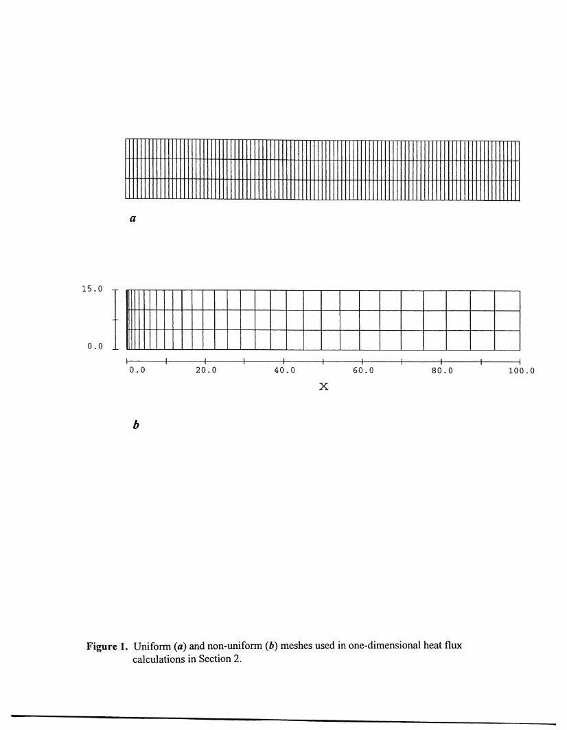
First, a comparison is made of the 'locally' implicit solution for Y=1.0 with the fully implicitone for y=1 and y=IO. Figure 2 shows that the fully implicit method is more accurate than the'locally' implicit one, even with a ten times larger time step. Also note that the fully implicitresult with y=I is not as accurate as the explicit one. This is typical of implicit solutionmethods.
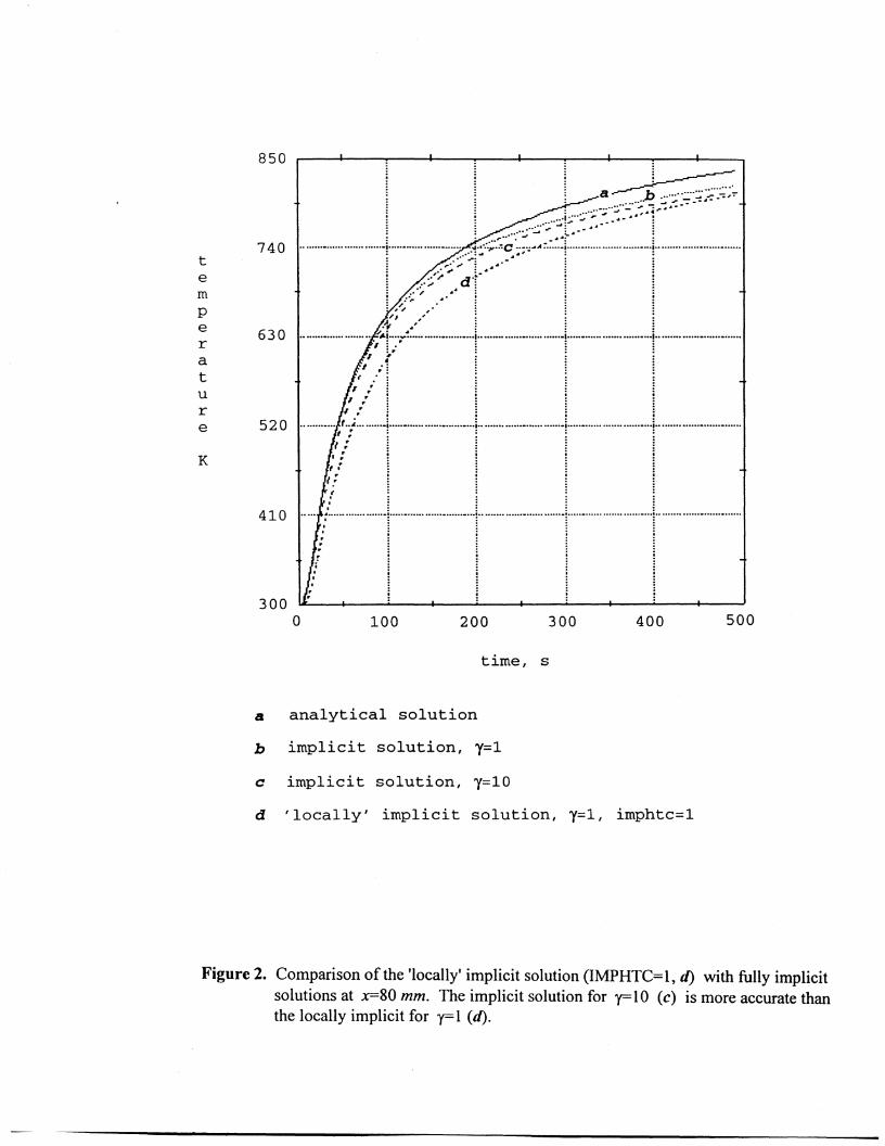
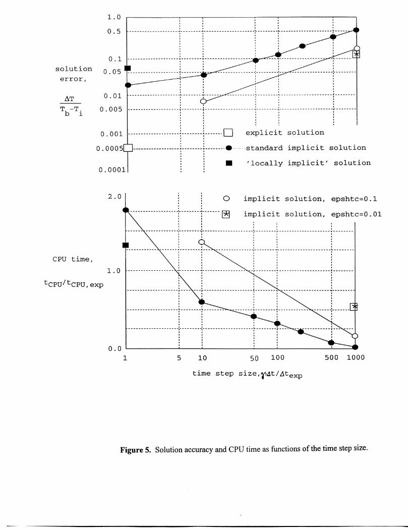
Figure 3 shows the influence of the value of the convergence criterion on the accuracy of theimplicit solution with y=10. The value of the criterion is altered using EPSHTC. AlthoughEPSHTC=O.I gives a more accurate solution than when the default value of 1.0 is used, theefficiency is worse than that of the original explicit simulation due to additional iterations neededto satisfy the criterion (see Fig. 5).
Figure 4 demonstrates the deterioration of accuracy of the implicit solution with the increaseof the time step. When the largest time step size was used, y=1000, only one time step wasrequired to complete the solution2
•
Figure 5 shows the dependence of the relative error, ~Timp, computed according to Eq. (13)and the CPU time (normalized to the CPU time of the explicit simulation, (CPU,exp) on the size ofthe normalized time step, y. The following can be concluded for this sample case:
1) The suggested convergence criterion, Eqs. (8)-(11), gives 95% to 90% accuracy fortime steps 10 to 50 times larger than the explicit time step size.
2) All simulations with yc.lO ran faster than the explicit solution.
3) Reduced values of EPSHTC give a more accurate solution but require more CPUtime. The gain in accuracy becomes smaller as EPSHTC decreases (11000). Obviouslythere is an optimum combination of the time step size and the convergence criterion toachieve acceptable accuracy and efficiency.
2 In cases when a steady state solution is required, the solution could be found iterativelyby using a large time step size. The accuracy of the steady state solution can be improved bydecreasing EPSHTC.
6
The maximum time step size that ensures a numerically stable transient explicit solution canbe interpreted as a period of time over which a heat wave propagates in space by no more thanone cell. When larger time steps are used in the implicit algorithms, these waves are allowed totravel farther in one time step. Over that period of time several heat waves may pass through thesame location in the flow, therefore, fluid energy and temperature at this location may experiencea complicated transient behavior over that same period of time. However, the temporal partialderivative in the energy equation is approximated with a first order differencing scheme (e. g. Eq.(3)) which effectively assumes linear energy variation during one time step. Therefore the useof large time steps in the implicit scheme leads to smoothing, or diffusing, of the solution and toa loss of accuracy in the transient solution.
The explicit stability limit does not only ensure stability, but also accuracy of transientsolutions. However, one could easily imagine a situation when the time step limit is small onlyin a small region of the mesh and is much larger elsewhere3
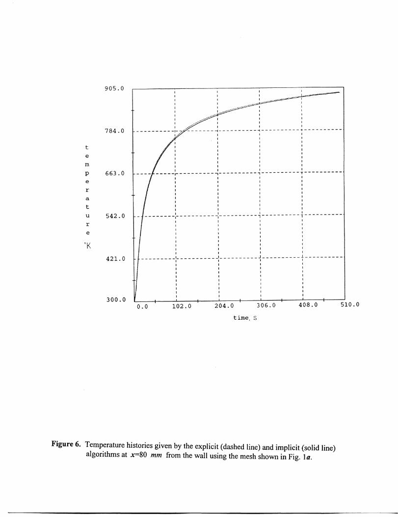
• Additionally, if temperatures arenot changing significantly in this region, then there is no need for a small time step size to ensureaccuracy there. In this case the use of the explicit time step stability limit is a shear waste ofcomputational effort. The implicit method could then be employed with a time step size close tothe stability limit in the larger part of the mesh, where the solution is transient, whilesignificantly exceeding the minimum stability limit. A sufficient accuracy would then beachieved throughout the mesh. Such a case can be generated by changing the mesh in thepresented example from the one shown in Fig. la to the one given in Fig. lb. In that case theexplicit stability limit is ~tmax = 0.0225 s. Running an implicit calculation at dl = 1.0 s (145)makes the calculation more than 17 times faster with little loss of accuracy as shown in Fig. 6.
5. Conclusions
The new, fully implicit, heat transfer algorithm adds flexibility to FLOW-3D in allowing theuser to run problems with heat transfer and conduction more efficiently by using large time steps.The convergence criterion is set automatically. The additional input variables, EPSHTC(namelist XPUT) and ITHTMX (namelist LIMITS), are designed to let the user adjust theconvergence criterion and the maximum iteration number, respectively, to achieve the bestresults in accuracy and efficiency of the solution. However, the default values of theseparameters are set to give the optimum results in most cases.
Users must be aware of possible significant truncation errors introduced by using time stepsconsiderably larger than the stability limit.ofthe explicit method, ~tmax. An input variableCONHT allows the user to limit the ratio of ~t/~tmax to the value of CONHT [1].
This could be, for example, because of non-uniformity of the mesh.7
3. RAPID SOLIDIFICATION SHRINKAGE MODEL
1. Overview
In recent years, more and more applications have been found for FLOW-3D in the castingindustry, where it is used to model such processes as high pressure injection, gravity and tiltpours, and centrifugal and squeeze castings. One such application is modeling volumetricshrinkage during solidification, which is a common cause of porosity defects leading to poormechanical properties of the final product. Here the code provides an efficient way to helpdesign a cost effective process that would minimize the occurrence of these defects.
The existing dynamic shrinkage model (DS) in FLOW-3D involves the solution of the fullsystem of fluid flow equations including Navier-Stokes equations (used when ISHRNK=l [1]).The model accounts for pressure and fluid flow changes in the liquid metal as it shrinks due tophase transformation. The occurrence and amount of porosity is controlled by a user specifiedvalue of the critical pressure, peA v, which effectively is the gas pressure in the cavities.
Despite being an accurate tool to study the porosity formation phenomena, the DS modelmay be computationally costly because at each time step th~ numerical algorithm involvesmomentum advection, viscous stress evaluation, velocity-pressure iterations, free surfaceadvection and, finally, heat transfer and conduction. The size of the time step, controlled byvarious stability criteria associated with fluid flow, may also be small compared to the totalsolidification time of the casting. The latter could be as long as hours for large sand castings.
The Rapid Solidification Shrinkage (RSS) model was recently added to FLOW-3D to providea simple tool to perform quick (rapid !) simulations of shrinkage in complicated castings. It isbased on the solution of only fluid and obstacle energy equations. No fluid flow equations aresolved by the model. Porosity is predicted by evaluating the volume of the solidificationshrinkage in each isolated liquid region in the casting at each time step. This volume is thensubtracted from the top of the liquid region in accordance to the amount of liquid metal availablein the cells from which the fluid is removed. The 'top' of a liquid region is defined by thedirection of gravity.
The feeding is defined by the value of the solidification drag force, F=Ku, where u is thelocal liquid metal velocity and K is the solidification drag coefficient. The latter is a function ofthe local solid fraction and its gradient. If the drag coefficient multiplied by the time step size,K~t, is above 106
, then no feeding occurs. Otherwise the shrinkage that occurred during theperiod of ~t is fully fed. This feeding criterion can be controlled by using the input variableTSDRG which is used as a multiplier when c.omputing K and defaults to 106
•
The amount of porosity, t1 V, is solely defined by the liquid and solid phase densities,PI and ps, respectively,
8
(14)
where ~ is the initial volume of liquid metal. If the densities are equal, no volumetric shrinkagewill occur.
The RSS model uses the following assumptions:
1) Metal volume can only decrease. For common metals and alloys, for which ps > PI, thismeans that phase transformation proceeds in the direction from liquid to solid. No volumewill be added to the metal in case of remelting.
2) Liquid metal free surfaces are flat and normal to the direction of gravity. This direction hasto be aligned with one of the coordinate axes.
3) Feeding occurs instantaneously during one time step.
4) Internal cavities open immediately when a liquid region is separated from the feeder.
5) Shrinkage in liquid regions attached to boundaries of type 3, 5 and 6 (continuitive, pressureand velocity boundaries, respectively) are always fed through these boundaries if the fluidtemperature at the boundaries is above solidus (TS 1), irrespective of the orientation of theboundaries relative to the feeding direction.
6) The amount of porosity is only controlled by the shrinkage; no gas evolution is included inthe model.
There are no limitations on the actual casting shape or configuration and metal and moldproperties in the RSS model. The main advantage of this model is that is it fast since it does notsolve any fluid flow equations. Its accuracy depends on how important the advective heattransfer is compared to thermal conduction, and whether significant gas evolution in the metal ispresent. The larger the role of the thermal conduction the better the accuracy of the model.Since no fluid flow equations are solved, fluid velocities are assumed to be zero. No dynamicfluid flow phenomena can therefore be modeled with the RSS model.
The RSS option is used if the value of ISHRNK is 2, in which case the heat-flow-onlyoption flag, IHONLY, is automatically set to 2 [1]. The direction of the feeding is chosen bythe code according to the values of the input variables GX, GY and GZ which denote gravityvector components. Only the maximum of the three is used, with the other two ignored. IfGX=GY=GZ=O.O (default), then the gravity is assumed in the negative z-direction.
9
2. Sub-time Stepping Algorithm for Implicit Option
When the implicit algorithm, described in Section 2, is employed the use of a large time stepmay cause significant inaccuracy in the predictions of the RSS model. This can be explained byconsidering the example of a one-dimensional plane solidification front moving in the positivex-direction. Since there is a sharp boundary between liquid and solid phases, all the volumetricshrinkage occurring at the front will be fed by the liquid ahead of the front.
In the numerical approximation we divide the domain into small control volumes (cells). Inour example when the solidification front is inside of a control volume, the cell behind the frontis already solid, while the one ahead of the front is still liquid. Therefore each solidifying cellwill have a fully liquid neighbor from which it can be fed. If we restrict the front to advance atmost one cell during each time step, then all shrinkage in each control volume will be fed. Thiswill be a physically sound solution. However, if the time step is large, then the solidificationfront may advance a few cells in one time step and some of those cells may have no adjacentliquid cells to feed them at the time of solidification. This will lead to porosity in these cellswhich obviously is not correct.
A sub-time stepping procedure for the RS~ option has been developed to reduce the effect ofa large time step on porosity predictions. This is only used in conjunction with the implicit heattransfer algorithm. The essence of the procedure is to use a linear interpolation between theprevious and the current values of energy, En and En+l , respectively, to compute the solidfraction, volumetric shrinkage and feeding in each control volume at each sub-time step betweentimes t n and t n+ I .
The default size of the sub-time step is chosen to be equal to the explicit stability limit givenby Eq. (1) since it provides a good measure of the time scale of the energy fluxes in the system.The user may vary this setting by specifying an additional input variable CONSHR which servesas a multiplier for the min function in Eq.(I) (the default value is 0.45).
The condition
(15)
where ~T is the temperature difference between two neighboring cells and L is the latent heat,states that the conductive heat flux from a cell over the time period ~ts does not exceed the totallatent heat contained in the cell. This condition ensures that the solidification front does notadvance more than one cell in the period of time equal to the sub-time step ~ts. Equation (15) isnot a stability condition but is necessary to maintain the accuracy of the porosity predictions. If~ts is equal to the stability limit, Eq. (1), then Eq. (15) transforms to
(16)
10
2. Sub-time Stepping Algorithmfor Implicit Option
When the implicit algorithm, described in Section 2, is employed the use of a large time stepmay cause significant inaccuracy in the predictions of the RSS model. This can be explained byconsidering the example of a one-dimensional plane solidification front moving in the positivex-direction. Since there is a sharp boundary between liquid and solid phases, all the volumetricshrinkage occurring at the front will be fed by the liquid ahead of the front.
In the numerical approximation we divide the domain into small control volumes (cells). Inour example when the solidification front is inside of a control volume, the cell behind the frontis already solid, while the one ahead of the front is still liquid. Therefore each solidifying cellwill have a fully liquid neighbor from which it can be fed. If we restrict the front to advance atmost one cell during each time step, then all shrinkage in each control volume will be fed. Thiswill be a physically sound solution. However, if the time step is large, then the solidificationfront may advance a few cells in one time step and some of those cells may have no adjacentliquid cells to feed them at the time of solidification. This will lead to porosity in these cellswhich obviously is not correct.
A sub-time stepping procedure for the RS~ option has been developed to reduce the effect ofa large time step on porosity predictions. This is only used in conjunction with the implicit heattransfer algorithm. The essence of the procedure is to use a linear interpolation between theprevious and the current values of energy, En and En+l , respectively, to compute the solidfraction, volumetric shrinkage and feeding in each control volume at each sub-time step betweentimes tn and t n+1 .
The default size of the sub-time step is chosen to be equal to the explicit stability limit givenby Eq. (1) since it provides a good measure of the time scale of the energy fluxes in the system.The user may vary this setting by specifying an additional input variable CONSHR which servesas a multiplier for the min function in Eq.(I) (the default value is 0.45).
The condition
(15)
where f!T is the temperature difference between two neighboring cells and L is the latent heat,states that the conductive heat flux from a cell over the time period f!ts does not exceed the totallatent heat contained in the cell. This condition ensures that the solidification front does notadvance more than one cell in the period of time equal to the sub-time step f!ts • Equation (15) isnot a stability condition but is necessary to maintain the accuracy of the porosity predictions. Iff!ts is equal to the stability limit, Eq. (1), then Eq. (15) transforms to
(16)
10
where in the liquid, I1T can be approximated as the difference between the metal liquidus andsolidus temperatures,
(17)
For most metals the specific heat in the freezing range, C(T[- Ts ), constitutes less than 20% ofthe total latent heat, therefore the condition given by Eq. (16) is likely to ensure the accuracy ofthe sub-time stepping algorithm. However, there could be situations where Eq. (16) is notsatisfied because !1T is significantly larger than the estimate of Eq. (17). This could be the caseat metal/mold interfaces.
An additional input variable, NSTSHR (namelist LIMITS), is provided for the user to set themaximum number of sub-time steps. It defualts to 100. The use of this variable prevents thecode from spending too much time on sub-time stepping when I1ts becomes very small. In thatcase !1ts is increased to IINSTSHR of the actual time step.
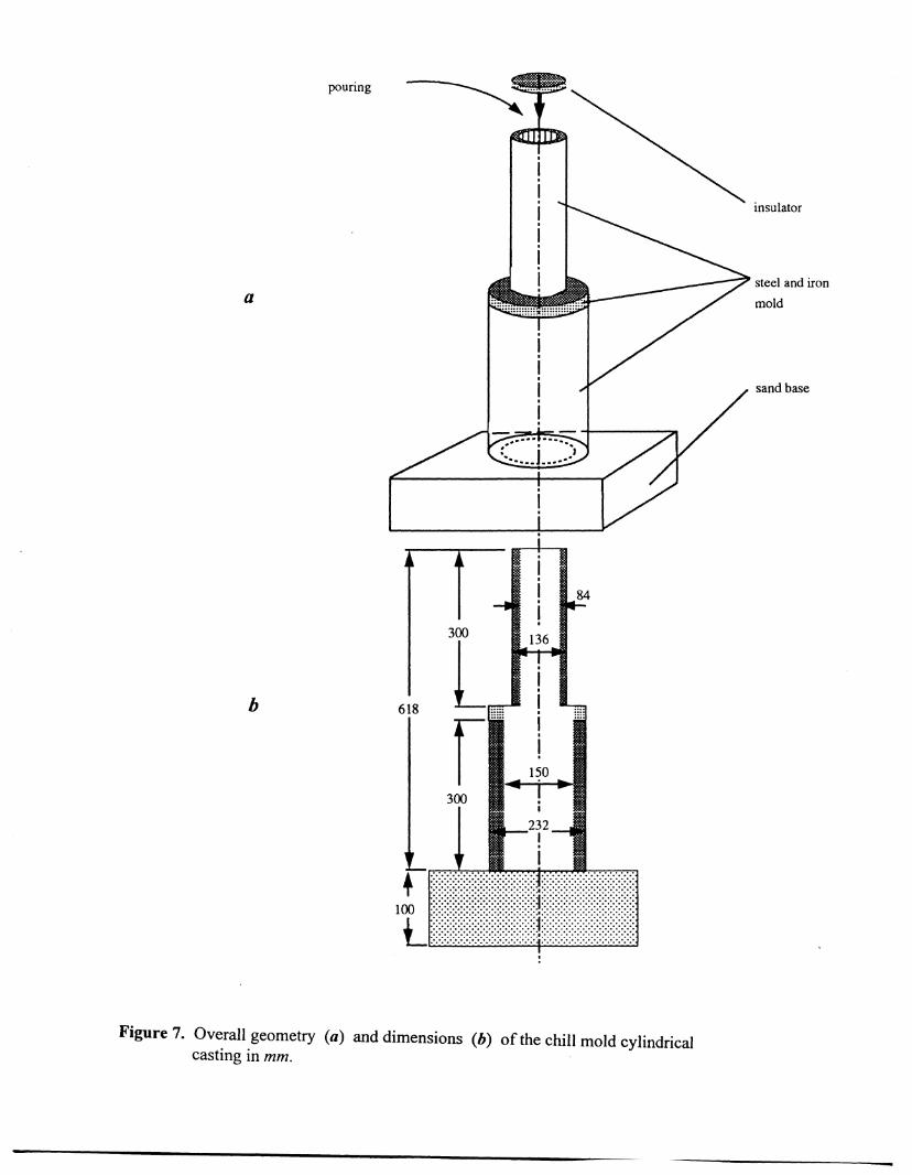
The test casting is a pure iron cylindrical ingot, the dimensions of which are shown in Fig. 7.The sides of the mold are made of steel with a sand pad at the bottom and an insulating lid at thetop. The pouring stage is omitted assuming uniform initial metal temperature at 1850°K andmold at 7500 K. The fluid properties and boundary conditions are
metal/chill heat transfer coefficient: 40000 W/m2K;metal/sand heat transfer coefficient: 1000 W/m2K;
chill mold constant temperature: 75ooK;
sand conductivity: 0.6 WlmK;sand density-specific heat product: 150000 Jim 3K.
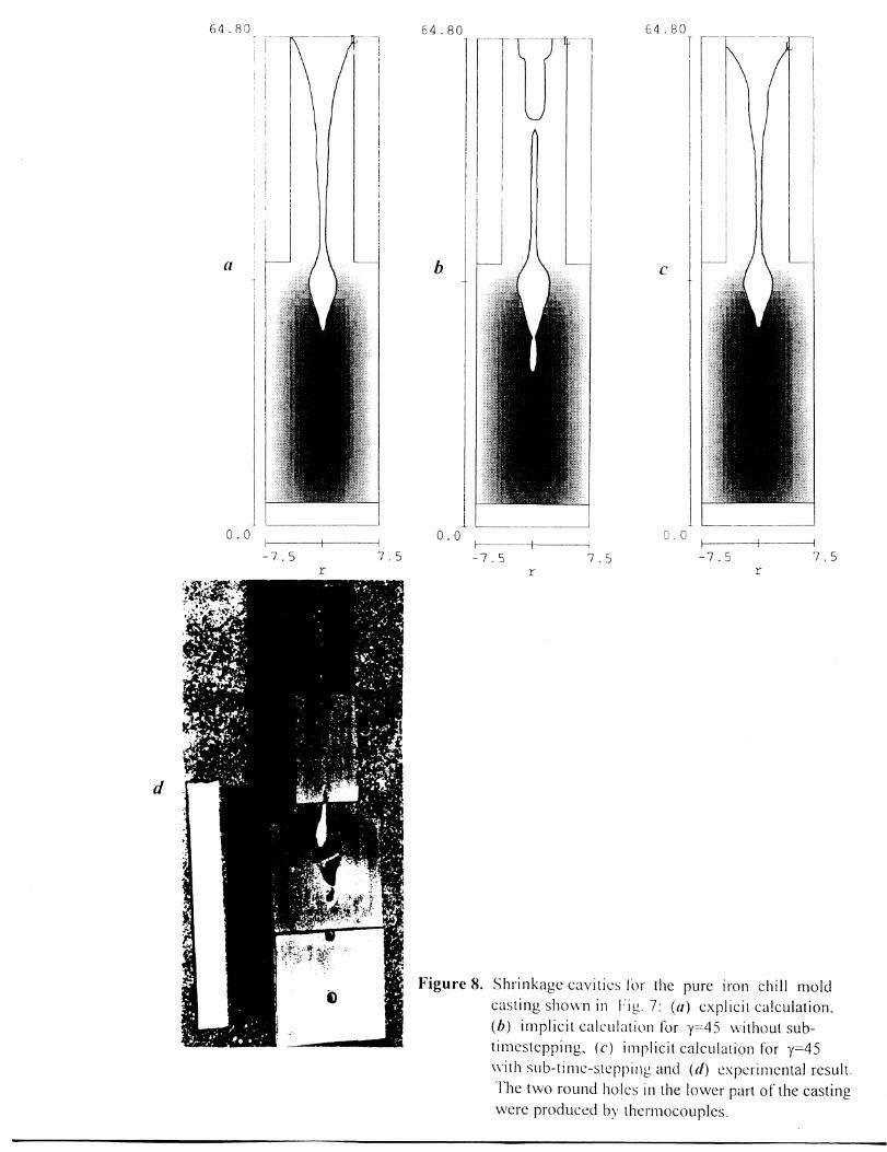
Figures 8a-8e show results of three simulations using the RSS model compared with anexperimental casting, Fig. 8d. The first simulation was run with the explicit algorithm. Thepredicted shrinkage cavity, Fig. 8a, is very similar to the experimental result, Fig. 8d. The timestep used was equal to 0.495 s (stability limit). Figure 8b shows the result of an implicitsimulation with !1t = 15 s and no sub-time stepping for the RSS model. The predicted cavity isdistorted in shape and extends much deeper than the explicit calculation result. Finally, Fig. 8eshows the result of an implicit simulation with the same time step as in the previous one but with
11
sub-time stepping at ~ts = 0.495 s. The predicted cavity in this case is very similar to the onegiven by the explicit simulation.
The explicit simulation took 53 CPU seconds to complete. The implicit simulation withoutsub-time stepping took 26 CPU seconds and the third simulation required 33 seconds. Despitethe fact that the RSS model had to be sub-cycled more than 30 times during each normal timestep in the third calculation, it took only 27% more time to compute than the implicit calculationwithout sub-time stepping.
3. Conclusions
The RSS model allows users to do efficient and accurate simulations of solidificationshrinkage porosity. Feeding occurs as a combined effect of gravity and conditions at meshboundaries. The latter takes into account possible feeding through the gating system of thecasting, e. g. due to an applied pressure at the gates in high pressure die castings. A sub-timestepping algorithm used in conjunction with the implicit heat transfer option ensures accuracy ofthe RSS model results even when large time step sizes are used to solve the energy equation.
4. HEAT TRANSFER AND CONDUCTION
1. Overview
Care must be taken to resolve areas where the flow variables have steep gradients.Discontinuity surfaces and internal boundaries represent such areas. The VOF method, forexample, allows one to resolve a free surface boundary inside a computational mesh cell and setboundary conditions in the cell according to the amount of fluid in it and the surface orientation[5]. Another example is the use of the FAVOR method to describe the obstacle surfaces insidemesh cells [6,7]. The FAVOR method requires fewer cells to r~present a sphere, for example,than if a stepwise approach were employed.
An extension of the FAVOR method has been made to improve the accuracy of metaVmoldheat transfer calculations, taking into account that cell-centered nodes do not, in general, lie onthe interface. The idea of the new addition is to use linear interpolation of the temperaturebetween a cell node and the location of the metal/mold interface to obtain metal and moldtemperatures at the interface. These temperatures can then be used to compute the heat flux atthe interface.
2. Outline of The Improved Algorithm
The accuracy of the present algorithm for metal/mold heat transfer is improved by assuming alinear profile of the temperature between the interface and the nearest cell node in the normaldirection to the interface.
12
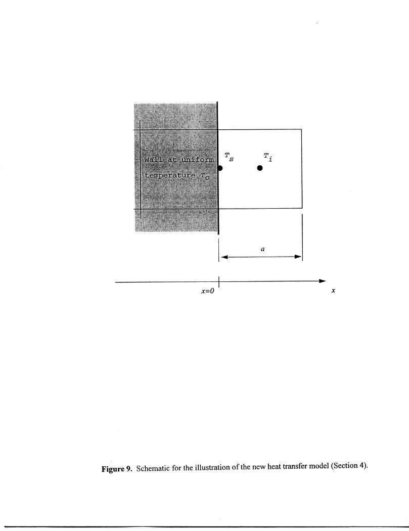
Let us consider a heat flow between a fluid cell i of size a and a wall. The wall has a fixedtemperature To. Suppose for simplicity that the fluid/wall interface lies exactly on the left cellface as shown in Fig. 9. For the heat balance in these two cells we have
dT j 2kPCa- == -(T - T·)dt Q S I
(18)
where T; is the cell-centered fluid temperature and T\. the fluid temperature at the interface.Fluxes in Eq. (18) are computed per unit area. The first ofEq. (18) describes conductive heattransfer between cell node i and the fluid/wall interface with the first order numerical
approximation of the temperature gradient, ~~. The second equation states the continuity o~ theinterfacial heat flux.
Equation (18) yields the temperature ofthejluid side of the interface
2kT - hTo+{iT;S - h+'l:!
a
and for the nodal temperature of cell i we have
where
(19)
(20)
(21)
Continuity of heat flux at the interface allowed us to exclude the surface temperature, Ts,
from the equations. This resulted in a modified expression for the heat transfer coefficient. Thevalue of heff is smaller than that of h since it takes into account the thermal resistance of thefluid layer between the interface and the cell node. This results in a larger value of the time stepstability limit for the explicit interfacial heat transfer algorithm. The distance a can be referredto as the distance that the heat has to penetrate into the cell to reach its center (the heatpenetration depth).
To check the accuracy of the modified expression for the interfacial heat flux, let us assumethat
(22)
13
is the exact heat flux through the interface since both To and Tsare surface temperatures. Usingthe Taylor expansion for Tj about x=O, which marks the location of the interface, we have forthe original expression for the heat flux, Q"
where equation
(24)
was used. Equation (23) shows that QI is first order accurate with respect to the cell size a.For liquid lead for which
h=17,000 W/m2K,k=15.4 W/mK
and a cell size a=2 mm the first order term is of the same order of magnitude as the zeroth orderterm, that is the error in the flux evaluation given by Eq. (23) of is about 100% of the actual flux.If the fluid represents sand for which the typical values are
h=I,OOO W/m2K,k=O.75 W/mK,a=5 mm
the first order term is more than three times larger than the zeroth order term. The basicalgorithm in the form of Eq. (23) effectively represents the interface by a row of cells with anon-zero volume. Therefore the interface has a thermal capacity proportional to the cell layerthickness and the fluid specific heat. Since interfacial cell sizes and interface geometry may varyacross the computational domain, the value of Ql becomes strongly mesh dependent.
If heff, given by Eq. (21), is used in Eq. (23) instead of h, then the heat flux, Q2 becomes
(25)
with a second order truncation error.
In general, the larger the value of ~ the more accurate is the modified method compared tothe original one. The higher order accuracy for the new method also implies reduced dependenceof the computed heat flux on the cell size a.
Generally, the first and second derivatives of temperature at the interface have opposite signs,therefore, the lowest order truncation errors in QI and Q2' Eqs. (23) and (25), are also ofopposite signs: QI overestimates the flux and Q2 underestimates it.
14
-----------------------------------------
For partially blocked cells the procedure is similar. However, instead of using thecell-centered temperature, Tj, the conductive heat flux is evaluated between the interface and thegeometrical center of the fluid region in the cell. In a one-dimensional case this results inreplacing the heat penetration depth a in Eq. (21) with aVF, where VF is the open volumefunction in the cell.
Only the fluid side of the interface has been considered so far. A similar procedure applied toboth open and blocked parts of an interfacial cell yields the effective heat transfer coefficient,hejf,
(26)
where indices 1 and 2 refer to the metal and mold at the interface and aJ and a2 denote heatpenetration depths in the two materials. Equation (26) implies the net heat transfer is limited bythe largest of the thermal resistances of the metal, mold and interface.
Conductive terms in the fluid and obstacle energy equations are also modified to accountmore accurately for temperature gradients in partially blocked cells.
3. Examples
As a simple test for the modification, a problem of transient one-dimensional heat flux into asemi-infinite sand mold has been considered. The boundary of the sand is at x=O and theboundary condition at it is
h[To - T(O, t)] = -k~~Ix=o (27)
where h and k are constant parameters and To is a constant ambient temperature. Initially thesand is at a uniform temperature Till. The analytical solution for T(x,t), t >0 and x >0 is [8]
For the numerical simulation the length of the sand domain was set at 200 mm, which was agood approximation of semi-infinity during the first hour of the simulation for
Density: p=1,500 kg/m3;
Specific Heat: C=1675 J/kgK;Thermal Conductivity: k=O.75 W/mK;Heat Transfer Coefficient: h=l,OOO W/m2K.
15
--~ --------------------------------------
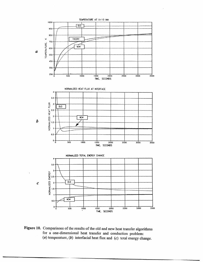
A uniform mesh with a 20 mm spacing was employed to solve the energy equation in thesand. The coarseness of the mesh was used to magnify the differences between the results of theold and new methods.
Figure lOa shows temperature histories computed at the center of the interfacial cell (at x=IOmm from the interface) compared with the analytical solution. The result of the old heat transfer
method is obviously less accurate. More over, it does not even converge to the analyticalsolution at the end of the simulation at (=3500 s. In contrast, the temperature predicted usingthe modified algorithm is much closer to the analytical solution and practically coincides with itat the end of the simulation.
Figure lOb shows the ratio of predicted to analytical heat fluxes (i.e. normalized heta flow) atthe interface. It can be seen that the old method largely overpredicts the heat flux at the initialstage of the simulation, « 150 S, while the new one underestimates it in the same period oftime.
Finally, predicted, normalized total energies fluxed through the interface are plotted in Fig.IOc. The result of the new method converges to the analytical solution much faster as thesimulation progresses than the one computed using the old method. At the end of the simulation,(=3500 S, the energy predicted by the old method is still 30% above the analytical solution,while the new method is practically identical to the theoretical result.
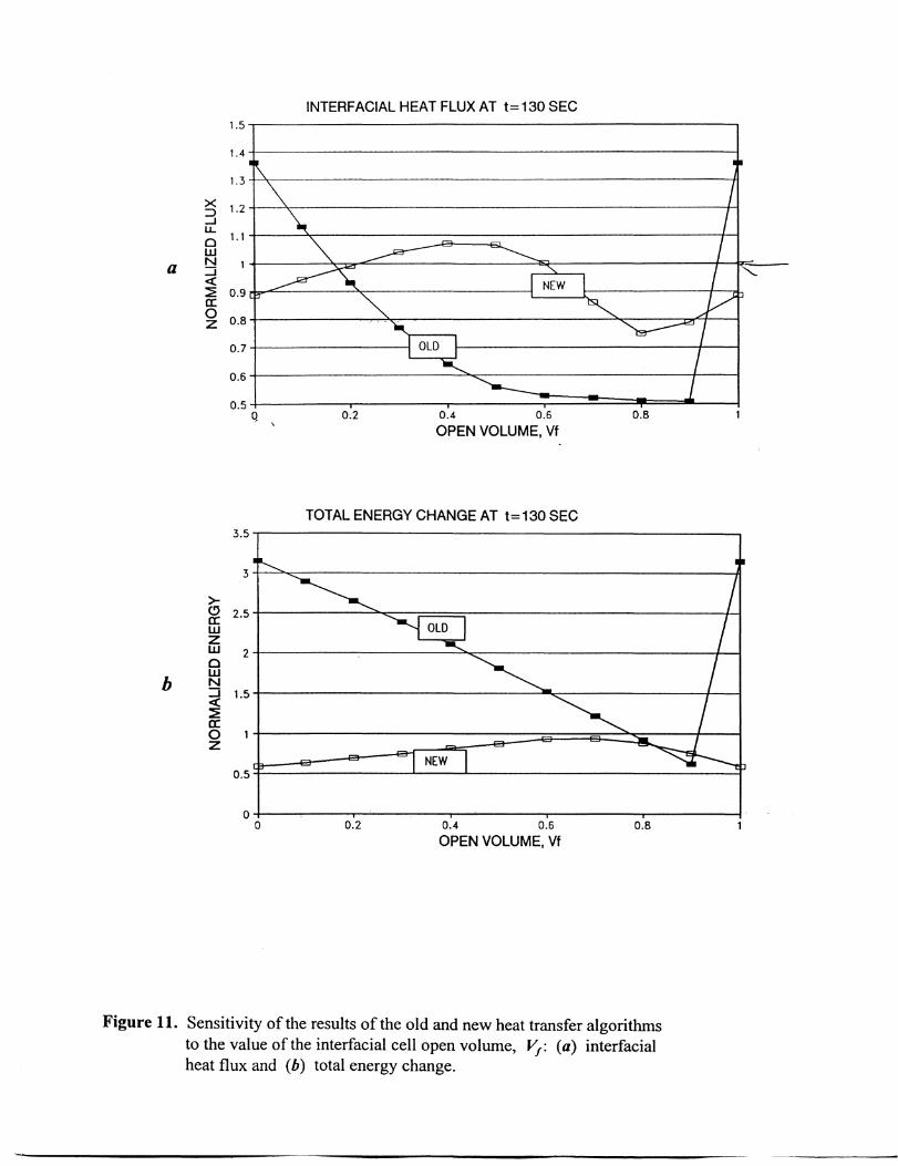
The results in this section are computed for a case when the fluid/wall interface lies exactly ona mesh face. What happens if we place the interface inside a mesh cell and keep the sameresolution? Figures Iia and lIb show the interfacial heat flux and the total energy fluxedthrough the interface at (=130 S from the beginning of the simulation, as predicted by the twomethods and compared with the analytical solution, as a function of the fractional open volumein the cell, VF• It can be seen that the results of the old method for the heat flux vary by than50%, compared to the analytical solution, as VF changes between 0 and 1. At the same time thenew method predictions vary by about 15%, a significant impr9vement in accuracy.
The error is still substantial with the improved method because of the coarseness of the meshused for this test, tu = 20 mm. These errors can be significantly reduced by using a finer mesh.A more typical grid spacing employed when computing heat fluxes in sand are in the range of 2to 5 mm. According to Eq. (25), truncation errors in evaluating the interfacial heat flux decreaseas tu2 , therefore, by changing tu from 20 to 5 mm the maximum error should be decreasedfrom 15% to less than 1%. For tu = 2 mm the maximum error should be 0.15%. An actualsimulation for the latter case gave an error of 0.45%. It is larger than the estimated 0.15% due toadditional truncation errors introduced by the first-order discretization method employed in thecode for the conductive terms in the energy equation.
16
a
15.0
0.0
0.0
h
20.0 40.0
x60.0 80.0
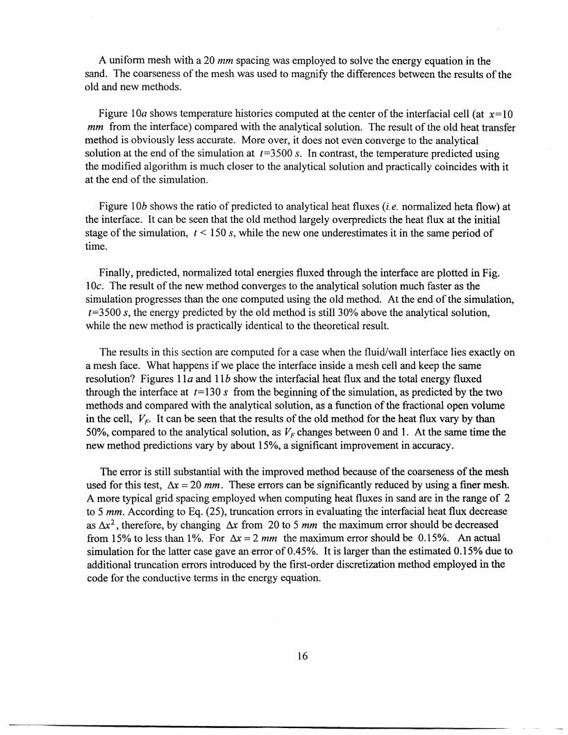
Figure 1. Uniform (a) and non-uniform (b) meshes used in one-dimensional heat fluxcalculations in Section 2.
.. ......•... t ..;..........•i............ . : : .t : :
1 : iI : ~t .p :
I.: ~t. ./ "\" ·················r , , .
. . . .
:/ iii I
520
300o
410
740
630
K
temperature
time, s
a analytical solution
b implicit solution, y=l
c implicit solution, y=10
d 'locally' implicit solution, y=l, imphtc=l
Figure 2. Comparison of the 'locally' implicit solution (IMPHTC=1, d) with fully implicitsolutions at x=80 mm. The implicit solution for y=10 (c) is more accurate thanthe locally implicit for y=1 (d).
500400300200100
.............. ···..··..····· ·· ·..·1 r- .
~ !~ ;
I :
.-:' --
• I; ••••••••••••••1" .
.. ~ : ~:::.-·::::::::·:...:.:·.·.·~.·.·.·r:: ~ .
./~).I: 1·· ;!. :
P",
:'" ::/~l..······..·..············..·1 : : ..
o300
410
850
740tempe
630rature
K
time, s
analytical solution
implicit solution,
implicit solution,
o-=10, epshtc=1.0
a=10, epshtc=O.l
Figure 3. Influence of the value of the convergence criterion on the implicit solutionaccuracy at x=80 mm. The convergence criterion is ten times smaller forthe more accurate solution (dashed line).
Figure 6. Temperature histories given by the explicit (dashed line) and implicit (solid line)algorithms at x=80 mm from the wall using the mesh shown in Fig. lao
pouring
a
h
300
618 L..... ....
r 150
300
insulator
steel and iron
mold
sand base
232I.I
Figure 7. Overall geometry (a) and dimensions (b) of the chill mold cylindricalcasting in mm.
64.80
a
0.0
64.80
b
0.0
64.80
c
0.0
-7.5r
7.5 -7.5r
7.5 -7.5r
7.5
d
Figure 8. Shrinkage cavities for the pure iron chill nloldcasting sho\vn in Fig. 7: (a) explicit calculation.,(b) inlpl icit calculation for y==45 \vithout subtinlestepping., (c) iJllplicit calculation for y==45\vith sub-tinlc-stepping and (ll) cxperinlcntal result.'rhe two round ho~es in the lower part of the casting\vere produced by thernlocouplcs.
x=o
T T.s ~
e
a
x
Figure 9. Schematic for the illustration of the new heat transfer model (Section 4).
3S0030002S001S00 2000
TIME, SECONDS1000SOO
2S0o
350 'I I
950
TEMPERATURE AT X= 10 MM1050-----r--I-----rt----,----,j----.,---I-----,;-------,
Figure 10. Comparisons of the results of the old and new heat transfer algorithmsfor a one-dimensional heat transfer and conduction problem:(a) temperature, (b) interfacial heat flux and (c) total energy change.
INTERFACIAL HEAT FLUX AT t=130 SEC1.5-----------------------------,
Figure 11. Sensitivity of the results of the old and new heat transfer algorithmsto the value of the interfacial cell open volume, VI: (a) interfacialheat flux and (b) total energy change.
4. Conclusions
The modified method is more accurate than the original one because it resolves thetemperature profile in the interfacial cells by a linear function, instead of the uniform temperatureused previously. In addition, the results of the new method are less dependent on the position ofthe fluid/obstacle interface inside mesh cells. This is important for accurate evaluation of theinterfacial heat fluxes for complicated obstacle geometries.
The main assumptions in the new algorithm are:
1) The interface has no heat capacity, i. e. heat fluxes on both sides of the interface areequal;
2) The temperature profile between the interface and the center of the cell open (orblocked) volume is linear as a consequence of the first order numericalapproximation for the heat conduction terms at the boundaries.
The linear interpolation allows one to have two temperatures, fluid and obstacle, exactly at theinterface. No differential equations have to be solved for these temperatures. As a consequence,this modification of the basic FLOW-3D algorithm does not require any additionalcomputational effort. The modified heat transfer coefficients are automatically precomputed atthe preprocessor level since the geometry does not change during a simulation involving heattransfer.
3. C.W. Hirt and C.L.Bronisz, 'On the Computation of Righly Viscous Flows,' Flow ScienceTechnical Note #31, Los Alamos, August 1991 (FSI-91-TN31).
4. J.M.Ortega and W.C.Rheinboldt, 'Iterative Solution ofNonlinear Equations in SeveralVariables,' Academic Press, New York, 1970.
5. C.W. Rirt and B.D. Nichols, 'Volume of Fluid (VOF) Method for the Dynamics of FreeBoundaries,' Journal of Computational Physics, 39, pp 201-225,1981.
6. C.W. Rirt and J.M. Sicilian, 'A Porosity Technique for the Definition of Obstacles inRectangular·Cell Meshes,' Fourth International Conference on Ship Hydrodynamics,Washington, DC, September 1985.