HAL Id: lirmm-00539838https://hal-lirmm.ccsd.cnrs.fr/lirmm-00539838

Submitted on 6 Dec 2010

HAL is a multi-disciplinary open accessarchive for the deposit and dissemination of sci-entific research documents, whether they are pub-lished or not. The documents may come fromteaching and research institutions in France orabroad, or from public or private research centers.

L’archive ouverte pluridisciplinaire HAL, estdestinée au dépôt et à la diffusion de documentsscientifiques de niveau recherche, publiés ou non,émanant des établissements d’enseignement et derecherche français ou étrangers, des laboratoirespublics ou privés.

Enhancing PKM Accuracy by Separating Actuation andMeasurement: A 3DOF Case Study

David Corbel, Olivier Company, Sébastien Krut, François Pierrot

To cite this version:David Corbel, Olivier Company, Sébastien Krut, François Pierrot. Enhancing PKM Accuracy bySeparating Actuation and Measurement: A 3DOF Case Study. Journal of Mechanisms and Robotics,American Society of Mechanical Engineers, 2010, 2 (3), pp.0310008. 10.1115/1.4001779. lirmm-00539838

Enhancing PKM accuracy by separating actuation and

measurement. A 3-dof case study.

David Corbel, Olivier Company, Sebastien Krut and Francois Pierrot∗

LIRMM, Univ. Montpellier 2, CNRS

161, rue Ada, 34392 Montpellier, France

Abstract

This paper propose an approach for enhancing PKM accuracy by separating actua-

tion and measurement. The interest of Separation Actuation & Measurement concept

(SAM) is exposed and a definition of sensor redundancy used for designing the mea-

surement device is given. Then, the design of a parallel Machine-Tool (MT) prototype

with a independent measuring system, MoM3, is presented as well as the optimiza-

tion of its measuring system. Finally, the control schemes used on the prototype are

presented and the experimental results show the efficiency of SAM applied to a MT.

1 Introduction

Designing a fast, accurate and stiff Machine-tool (MT) is really a hard task. To take up

this challenge, MT designers took their inspiration from recent advances in robot kinematic

architectures, in particular Parallel Kinematics Machines (PKMs) [1]. PKMs are already

used with success in some industrial domains1.

Nowadays, two well known types of PKMs are transferred to the MT industry:

∗Corresponding author: pierrot@lirmm.fr1http://www.parallemic.org/WhosWho/CompPKM.html

1

• The hexapods, where six variable length struts link a traveling plate to a base. The

first PKM belonging to this family was proposed by Gough [2].

• The Delta robot, invented by Prof Clavel [3], which is a lower mobility PKM (displace-

ments of the traveling plate are restricted to three translations).

The Variax was the first MT inspired by the hexapod architecture [4], and until today,

a lot of industrial machines based on this architecture are built: Octahedral Hexapod by

Ingersoll, the P1000/P2000/P3000 Hexapods by PRSCO, or the HexaM by Toyoda (even

though HexaM is not strictly speaking an ”hexapod” since it is not made with 6 telescopic

legs). Concerning the Delta kinematics, its version with linear actuators is used on MTs

as for UraneSX [5] that can reach up to 5g in its workspace or Quickstep by Krause &

Mauser [6].

The main interest for using parallel architecture on MTs is to take advantage of their

high dynamical capabilities. These architectures can reach high accelerations because of the

light weight of their movable elements compared to serial architectures.

However, whatever the architecture is, geometrical calibration is required to get the best

accuracy. The calibration tries to identify model parameters that enhance the machine

accuracy [7]. Once these parameters are identified, the model runs ”open loop”, ie the

machine behavior is expected to be the one that has been modeled and identified whatever

the stresses in machine components are. For Cartesian classical MTs, the identification

can be done axis per axis. Parameter identification can be very accurate as the problem

is decoupled. Identifying PKM parameters according to this principle is not possible as all

axes are coupled in the model. A full calibration of the model must be done, but it always

2

ends in a compromise between the number of parameters and the numerical stability [8].

Moreover, for MTs based on parallel architecture, geometrical calibration is not sufficient.

To benefit from the high dynamics of the parallel architecture, the use of light elements is

necessary and therefore the stiffness of the machine can sometimes be low [9]. This low

stiffness of parallel mechanisms is a drawback when they are used in MTs. One solution

consists to add redundancy in the architecture [10]. Another solution consists in modeling

the deformations using an elastic model of the structure [11] [12] [13]. This solution is

interesting to compensate the gravity effects or when the efforts on the end-effector are

known but it is seldom the case.

The basic problem in machining is to impose accurate end-effector positioning regarding

the part to be machined. The best way to deal with accuracy is to always be able to know

the end-effector pose (position and orientation) relative to the part accurately, ie with a

quality as close as possible to the metrological one. This can be done by measuring directly

the end-effector pose. One way to proceed is to use non-contact full pose measurement

system, like vision system [14]. According to [15], 3D visual servoing reduces the complexity

of parallel robot Cartesian control. But there is still ongoing research on this topic and, even

if algorithms are available, they are not able today to guarantee the requested resolution on

the whole workspace of the machine. Moreover, the refreshment rate is not high enough for

the control loop, but it is still a promising way of research for the future.

However, visual servoing illustrates the idea of having independence between the mea-

surement chain and the actuation chain. The principle of Separation between Actuation

and Measurement (SAM) relies on this independence. SAM allows to guarantee the exact

measurement of the end-effector pose therefore a very accurate end-effector positioning.

3

First, the principle of SAM is explained in section 2. To prove the feasibility and the

efficiency of this concept an actuated PKM (a Delta robot) combined with a passive mea-

suring PKM (a Gough platform) is presented in section 4. Then, the optimization of the

Gough platform is recalled in section 5. Finally, the control laws used on the mechanism are

described (section 6) and the experimental results are shown (section 7).

2 Separation between actuation and measurement

2.1 Motivations

On classical serial or parallel MTs, measuring systems are close to actuators (e.g.: encoders

attached to the motors) or close to guideways (e.g.: linear scale on a prismatic joint) (Fig.

1a and 2a). In most cases, these measuring systems do not give any information about

(i) assembly errors (Fig. 1b and 2b) or (ii) deformations of the structure (Fig. 1c, 2c).

Fig. 3 illustrates this problem for the general case: on a classical machine, with serial

or parallel kinematics, most components involved in the measurement chain have to sustain

loads coming from the process (e.g.: cutting forces) and suffer from the same assembly errors

or thermal effects because they belong to the very same force and motion transmission chain.

The concept of SAM comes from these observations. The idea is to create a measur-

ing system as independent as possible from the force transmission system and as sensitive

as possible to the assembly errors and deformations of the mechanical structure. Ideally,

the measuring system must be linked only to the ground and the end-effector to insure

this independence (Fig. 4). This concept is not completely new: it has been described in

4

(a) (b) (c)

Figure 1: (a) Classical serial MT, (b) with assembly errors, (c) with deformations

(a) (b) (c)

Figure 2: (a) Parallel MT, (b) with assembly errors, (c) with deformations

earlier works. David used this concept for the design of a Coordinate Measuring Machine

(CMM) [16]; in seminal work by Hale and Slocum several important principles and tech-

niques to design precision machines were proposed [17] [18], among which the SAM concept

for high precision machine-tools; Lahousse [19] resorted to the same principle for designing

a measuring device with nanometer resolution.

5

Figure 3: Classical association of actuation and measurement on robots

Figure 4: Metrology of robots with SAM

6

2.2 Actuation chain

Following the concept of SAM, the main function of the actuation chain is to generate and

transmit forces to move the end-effector.

As the position and orientation of the traveling plate are measured directly by an in-

dependent measuring system, even if some machining or assembly errors exist, they do not

influence the accuracy of the machine, as long as a control loop relying on these measures

can compensate for the errors.

However, the displacement resolution of the end-effector must be compatible with the

defined task and so backlashes and friction effects must by sufficiently low to insure this

compatibility.

2.3 Measurement chain

Some features concerning the measurement chain must be taken into account during the

design phase:

(i) The measuring system must measure directly (or almost directly) the end-effector pose.

(ii) The acquisition frequency must be compatible with real-time control needs (typically:

above 1kHz).

(iii) The positioning capabilities (resolution, repeatability and accuracy) of the measuring

system must be compatible with the positioning capabilities required for the task to

be achieved.

(iv) The measuring system must transmit no force.

7

(v) The measuring system must not interfere with the actuated mechanism.

Measurement systems can be split into two categories:

• without contact; this could be LASER based sensors or cameras for artificial vision;

• with contact; this could be serial measurement arms or systems with parallel kinemat-

ics.

A key question regarding the measuring system is: how many pieces of information are

necessary to control accurately the machine? Answering this question requires the definition

of sensor redundancy.

3 Sensor redundancy

3.1 Definition

Let us define :

• C is the sensor space dimension. It corresponds to the number of independent measures

given by the set of sensors.

• M is the dimension of space wherein the end-effector evolves.

• D is the number of the robot degrees of freedom (dof ).

• O is the spatiality2 of the traveling plate.

2Number of independent relative velocities between the base and end-effector of the machine [20]

8

Definition : The degree of sensor redundancy (dosr) is equal to C − (M − O +D).

Then, three cases can be distinguished :

• dosr < 0, the mechanism is ”under-measured”;

• dosr = 0, the mechanism is ”iso-measured”;

• dosr > 0, the mechanism is ”over-measured”, and so, there is a sensor redundancy.

One important aspect of this definition is how the variable M is considered. Two cases

have to be analyzed: ”perfect” case and ”imperfect” case. In the ”perfect” case, M is equal

to the spatiality of the mechanism, O. In the ”imperfect case”, M is larger than O. Let’s

take some examples to illustrate the definition.

3.2 Examples

3.2.1 1D example

Fig. 5 shows a solid which moves along a prismatic joint (D = 1, O = 1). In the ”perfect”

case, only 1 measure (M = 1) is sufficient to have an ”iso-measured” mechanism: dosr

= 1 − (1 − 1 + 1) = 0. In an ”imperfect” case, the solid may evolve not only along x axis

but have some parasitical movements along y axis (Fig. 5b). Then, M would be equal to 2

and dosr becomes negative. In such a case, additional measures should be added to recover

”iso-measurement”.

9

(a) ”perfect” case (b) ”non perfect” case

Figure 5: Solid along a prismatic joint

3.2.2 Kinematic redundancy

The definition of the sensor redundancy given in this paper can deal with kinematically

redundant mechanisms and mechanisms with actuation redundancy. Let’s start with kine-

matically redundant mechanisms.

First, the definition of kinematic redundancy is recalled: kinematic redundancy appears

when, for a given end-effector velocity and a given pose, there is an infinite number of

corresponding joint velocities.

Figure 6: Kinematically redundant parallel manipulator

As an example, Fig. 6 shows a kinematically redundant mechanism with 4 dof and a

10

end-effector spatiality equal to 3 (D = 4, O = 3). The ”perfect” case is considered here

(M = O) and only the actuated revolute joint are measured (C = 4). For this mechanism,

the dosr is equal to 0. So, in the ”perfect” case, this kinematically redundant mechanism is

”iso-measured”, even though it is equipped with more sensors than its spatiality.

3.2.3 Actuation redundancy

The definition of actuation redundancy is the following: actuation redundancy appears when,

for a given force/wrench acting on the end-effector and a given pose, there is an infinite

number of corresponding joint forces/torques.

Figure 7: Parallel manipulator with actuation redundancy

As an example, Fig. 7 shows a mechanism with actuation redundancy with 3 dof and

a end-effector spatiality equal to 3 (D = 3, O = 3). The ”perfect” case is considered here

(M = O) and only the actuated revolute joints are measured (C = 4). For this mechanism,

the dosr is equal to 1. So, in the ”perfect” case, this mechanism with actuation redundancy

is ”over-measured”.

11

3.3 Conclusion

It will often be necessary to consider thatM is equal to 6 (position and orientation of the end-

effector in space) since it is difficult to cancel all the errors which cause parasitical movements.

But, if the parasitical movements are negligible compared with the required accuracy, then

the perfect case can be applied (M = O). Of course, the definition of dosr given here is

just a first indication of what is needed in terms of number of sensors. Designers have to

guarantee that the measures are independent and sensitive to the considered displacements

in order to provide an efficient control.

4 MoM3 : Parallel Machine-Tool with Independent

Measuring System

Fig. 2 has shown that PKM suffer from the same problems than their serial counterparts:

links and joints suffering from deformations due to process forces are included into the mea-

surement chain. It turns out that PKM might be good candidates for designing systems

relying on SAM. This section introduces a parallel machine which has been designed re-

specting the considerations exposed above.

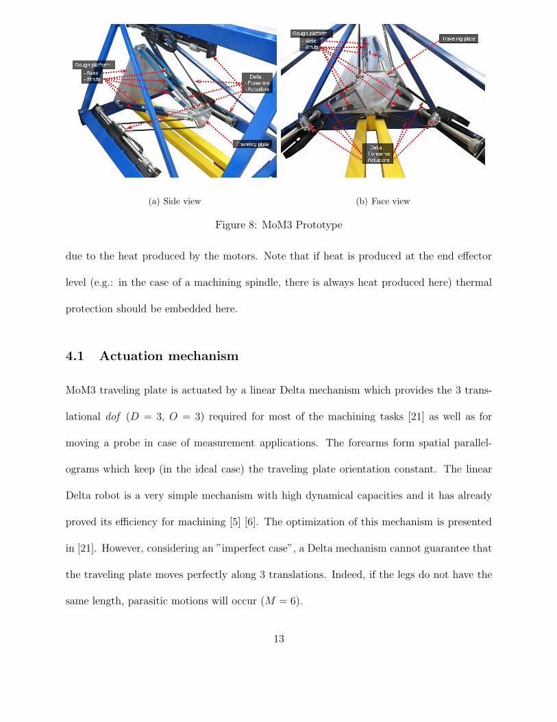
MoM3 is composed of a 3-dof actuated linear Delta mechanism and a 6-dof measuring

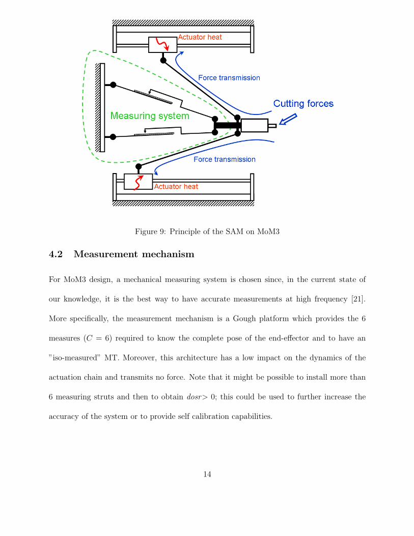
passive Gough platform (see prototype in Fig. 8). Figure 9 shows how SAM works on MoM3.

The forces applied on the end-effector are transmitted to the ground by the actuated chains

while the Gough platform measures directly the end-effector pose without transmitting any

force due to the process. The measurement device is also protected from the thermal effects

12

(a) Side view (b) Face view

Figure 8: MoM3 Prototype

due to the heat produced by the motors. Note that if heat is produced at the end effector

level (e.g.: in the case of a machining spindle, there is always heat produced here) thermal

protection should be embedded here.

4.1 Actuation mechanism

MoM3 traveling plate is actuated by a linear Delta mechanism which provides the 3 trans-

lational dof (D = 3, O = 3) required for most of the machining tasks [21] as well as for

moving a probe in case of measurement applications. The forearms form spatial parallel-

ograms which keep (in the ideal case) the traveling plate orientation constant. The linear

Delta robot is a very simple mechanism with high dynamical capacities and it has already

proved its efficiency for machining [5] [6]. The optimization of this mechanism is presented

in [21]. However, considering an ”imperfect case”, a Delta mechanism cannot guarantee that

the traveling plate moves perfectly along 3 translations. Indeed, if the legs do not have the

same length, parasitic motions will occur (M = 6).

13

Figure 9: Principle of the SAM on MoM3

4.2 Measurement mechanism

For MoM3 design, a mechanical measuring system is chosen since, in the current state of

our knowledge, it is the best way to have accurate measurements at high frequency [21].

More specifically, the measurement mechanism is a Gough platform which provides the 6

measures (C = 6) required to know the complete pose of the end-effector and to have an

”iso-measured” MT. Moreover, this architecture has a low impact on the dynamics of the

actuation chain and transmits no force. Note that it might be possible to install more than

6 measuring struts and then to obtain dosr> 0; this could be used to further increase the

accuracy of the system or to provide self calibration capabilities.

14

4.3 Measurement technology

The measuring struts are composed of telescopic legs with two parts: one mobile part and

one fixed part. A linear scale is placed on the mobile part and a scanning head is placed on

the fixed part (Fig. 10a). The linear scales have a resolution of 1 µm for this first prototype

but higher resolution scales are available on the market and could be installed as well. The

struts are linked to the base and end-effector by magnetic spherical joints which provide low

friction and very low positioning errors (below 1 µm).

One very important point is that the calibration of the Gough platform is very simple

thanks to the use of these measuring struts. Indeed, the struts can be calibrated one by one

with a calibration artefact (Fig. 10c). Moreover, the position of the spherical joint centers

can be determined accurately with a CMM, since both the Gough platform fixed plate and

the traveling plate are small parts which can easily be dismounted and placed on a CMM.

(a) Gough platform strut sketch (b) Gough platform strut in the calibration arte-

fact. This equipment has been designed following

our specifications by Symetrie Co. Nımes, France.

Figure 10: Gough platform strut and calibration device

15

5 Optimization of the Gough platform

5.1 Introduction

This section presents the optimization of the Gough platform. The features studied here

are the positioning capabilities of the Gough platform. As explained before, the measuring

system must have good positioning capabilities: repeatability, resolution and accuracy. These

capabilities depend on several factors. Some factors can be controlled during the design

process while others cannot. Let’s see this for each positioning capability.

First of all, repeatability is extremely dependent on the realization of the joints, the

choice of the mechanical elements and the quality of the control. Backlash or friction on the

joints can decrease repeatability.

Concerning the machine accuracy, calibration is required to eliminate the positioning

errors due to manufacturing and assembly errors. On the designed Gough platform, the

calibration is very simple as explained above. Other sources of errors exist as compliance

which can be modeled and identified [13]. In our case, the compliance of the Gough platform

is neglected since the elements of Gough platform are supposed not to be stressed (except

the weight of the struts which is neglected).

Finally, the last capability is the resolution of the mechanism. The first elements which

get involved in the mechanism resolution are the active-joint encoders resolution and the

controller quality. An other element is the mechanism architecture which is determined

during the design phase. Indeed, the transformation between the actuator and end-effector

movements depends on the dimensions of the mechanical elements. So, the mechanism

theoretical resolution can be improved by an optimization of these dimensions.

16

The goal of the optimization is to improve the measurement resolution at the tool level.

In other words, considering the resolution of the leg encoders, the resolution at the tool level

is the minimal displacement of the tool which can be detected by the measuring device. The

objective is to have a measuring device which can detect the smallest possible displacement

of the tool. The optimization consists in finding the dimensions of the Gough platform which

allow to reach this objective. As far as we know, the term “resolution” is correctly defined

only for mono-dimensional problems and has, so far, no universally accepted definition for

multi-dof cases. We try in the following section to propose a “worst case view” of this issue

which will give an upper bound of the smallest possible tool displacement.

5.2 Modeling of the Gough platform

Fig. 11 shows the parameters of the Gough platform. Points Ai (Bi, respectively) which

represent the centers of the spherical joints on the base (on the traveling plate) are placed

on a circle of radius rb (rtp). Then, three lines passing by the base center O and the traveling

plate center Eh and separated by an angle α0 are defined. Points Ai (Bi) are then located

symmetrically to these lines, two by two, with an angle of αb (αtp).

The measured-joint variables are defined by the Gough platform strut lengths noted li

(i ∈ [1, 6]). The pose xh of the platform is defined by the coordinates xh,yh,zh of the traveling

plate center Eh in the base frame Rb together with 3 angles (yaw, pitch, and roll) ψh,θh,φh

that allow to calculate the rotation between the base frame Rb and the traveling plate frame

Rtp.

For the optimization of the Gough platform, the positioning errors ∆xh and the length

17

(a) 3D view (b) Top view

Figure 11: Geometrical parameters of the Gough platform

measurement errors ∆l are supposed to be small enough to write an approximation of the

error model such as:

∆xh ≈ Jh(P ,xh)∆l, (1)

where P = [rb, rtp, αb, αtp]T is the vector of the geometrical parameters and Jh(P ,xh) is

the Jacobian matrix of the Gough platform. Only the inverse of the Jacobian matrix has an

analytical form which can be calculated as follows:

J−1h =

u1 −u1 × B1Eh

......

u6 −u6 × B6Eh

, (2)

with

ui =AiBi

li. (3)

18

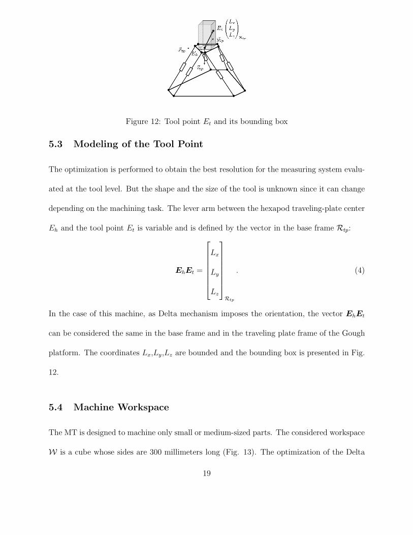
Figure 12: Tool point Et and its bounding box

5.3 Modeling of the Tool Point

The optimization is performed to obtain the best resolution for the measuring system evalu-

ated at the tool level. But the shape and the size of the tool is unknown since it can change

depending on the machining task. The lever arm between the hexapod traveling-plate center

Eh and the tool point Et is variable and is defined by the vector in the base frame Rtp:

EhEt =

Lx

Ly

Lz

Rtp

. (4)

In the case of this machine, as Delta mechanism imposes the orientation, the vector EhEt

can be considered the same in the base frame and in the traveling plate frame of the Gough

platform. The coordinates Lx,Ly,Lz are bounded and the bounding box is presented in Fig.

12.

5.4 Machine Workspace

The MT is designed to machine only small or medium-sized parts. The considered workspace

W is a cube whose sides are 300 millimeters long (Fig. 13). The optimization of the Delta

19

Figure 13: MT workspace W (300 × 300 × 300 mm3)

robot and the Gough platform is performed for this workspace.

5.5 Optimization criterion

Two phases are distinguished concerning the Gough platform optimization. First of all,

the optimization problem is analyzed considering the tool point as known. Then, the tool

bounding box will be considered.

5.5.1 Leg Encoder Errors

Any small displacement of the Gough platform traveling plate, in position ∆ph and orienta-

tion ∆rh, results in a small displacement of the considered tool point can be approximated

by ∆pt; this displacement is evaluated at first order as follows:

∆pt = ∆ph + ∆rh × EhEt, (5)

with

∆xh =

∆ph

∆rh

. (6)

20

From (1), the relation mapping the length measurement errors ∆l to the corresponding tool

positioning errors ∆pt can be written:

∆pt = JhP(P ,xh)∆l + JhR

(P ,xh)∆l × EhEt, (7)

with

Jh(P ,xh) =

JhP(P ,xh)

JhR(P ,xh)

. (8)

To simplify (7), the second term of its right member is rearranged as follows:

JhR∆l × EhEt = −EhEt × JhR

∆l

= −EhEtJhR∆l,

(9)

where EhEt represents the cross-product matrix.

A small change in the length of the six hexapod struts is mapped into a displacement for

the considered tool point by the following relation:

∆pt = Jt∆l, (10)

where

Jt = JhP− EhEtJhR

, (11)

is a 3×6 matrix.

Looking for the ’worst case’ requires to find the largest value of ‖∆pt‖ (Euclidean norm

of the vector ∆pt) when each measuring leg encoder suffers from an uncertainty of ε equal

to their resolution:

−ε < ∆li < ε. (12)

21

Due to the linearity of the system (10), for a given point of the workspace and for a given

tool point, the maximal value of ‖∆pt(P,Xh)‖ corresponds to the 26 possible combinations

corresponding to vectors ∆l whose components can be equal to +ǫ or −ǫ.

5.5.2 Unknown Tool Size

Now, for a given ∆l belonging to the 26 combinations, the fact that the tool point is consid-

ered inside a bounding box has to be taken into account.

Equation (10) can be developed as follows:

∆pt =

6∑

i=1

J1i∆li +6

∑

i=1

J5i∆liLz−6

∑

i=1

J6i∆liLy

6∑

i=1

J2i∆li +6

∑

i=1

J6i∆liLx−6

∑

i=1

J4i∆liLz

6∑

i=1

J3i∆li +6

∑

i=1

J4i∆liLy−6

∑

i=1

J5i∆liLx

, (13)

where Jji is the element at j-th row and i-th column of Jh.

The norm of ∆pt is given by:

‖∆pt‖ =(

(S1 + S5Lz − S6Ly)2

+ (S2 + S6Lx − S4Lz)2 + (S3 + S4Ly − S5Lx)

2)

1

2

,

(14)

with

Sj =6

∑

i=1

Jji∆li. (15)

The squared norm is then studied as a function of Lx,Ly and Lz:

f(Lx, Ly, Lz) = ‖∆pt‖2. (16)

Finding the maxima of function ‖∆pt‖ is equivalent to finding the maxima of function

‖∆pt‖2.

22

Briot [22] presents the mathematical background necessary to study this function. He

classifies four types of maximum (first, second, third and fourth kind) which are respectively

in the whole bounding box, or on the faces, or on the edges or on the corners of the bounding

box. Finally, the following functions must be studied:

f1 : (Lx, Ly, Lz) → f(Lx, Ly, Lz), f2 : (Ly, Lz) → f(Lxmin, Ly, Lz),

f3 : (Ly, Lz) → f(Lxmax, Ly, Lz), f4 : (Lx, Lz) → f(Lx, Lymin

, Lz),

f5 : (Lx, Lz) → f(Lx, Lymax, Lz), f6 : (Lx, Ly) → f(Lx, Ly, Lzmin

),

f7 : (Lx, Ly) → f(Lx, Ly, Lzmax), f8 : (Lz) → f(Lxmin

, Lymin, Lz),

f9 : (Lz) → f(Lxmin, Lymax

, Lz), f10 : (Lz) → f(Lxmax, Lymin

, Lz),

f11 : (Lz) → f(Lxmax, Lymax

, Lz), f12 : (Ly) → f(Lxmin, Ly, Lzmin

),

f13 : (Ly) → f(Lxmin, Ly, Lzmax

), f14 : (Ly) → f(Lxmax, Ly, Lzmin

),

f15 : (Ly) → f(Lxmax, Ly, Lzmax

), f16 : (Lx) → f(Lx, Lymin, Lzmin

),

f17 : (Lx) → f(Lx, Lymax, Lzmax

), f18 : (Lx) → f(Lx, Lymin, Lzmin

),

f19 : (Lx) → f(Lx, Lymax, Lzmax

),

where Lxmin, Lxmax

, Lymin, Lymax

, Lzmin, Lzmax

designate the minimal and the maximal

values of Lx, Ly, Lz.

The first function f1 reaches a maximum when its gradient is null and when its hessian

matrix is negative definite. The system of equations which described that the gradient is

23

null is:

S6(S2 + S6Lx − S4Lz) − S5(S3 + S4Ly − S5Lx) = 0

−S6(S1 + S5Lz − S6Ly) + S4(S3 + S4Ly − S5Lx) = 0

S5(S1 + S5Lz − S6Ly) − S4(S2 + S6Lx − S4Lz) = 0

(17)

The three equations of this system are not independent. This system represents the equation

of a line. Now, it is necessary to study the hessian matrix to qualify the critical points of

the function which belong to this line:

H(f1) =

2S52 + 2S62 −2S5S4 −2S6S4

−2S5S4 2S42 + 2S62 −2S6S5

−2S6S4 −2S6S5 2S42 + 2S52

. (18)

This matrix is constant whatever Lx, Ly and Lz. The determinant of this matrix is null and

its eigenvalues are σ1 = 0 and σ2 = σ3 = 2S46 + 2S2

5 + 2S24 . The matrix H(f1) is positive

semi-definite and the function f has no maximum of the first kind.

Then, the functions f2, . . . , f19 are treated as the first one, that is, analyzing their gradi-

ents and hessian matrix. It is determined that there is neither maximum of the second kind

nor maximum of the third kind.

Finally, only a maximum of the fourth kind exists and is on one of the eight corners of

the tool bounding box.

5.5.3 Global Optimization Criterion

Let ΩLx, ΩLy

, ΩLz, Ωl0 , Ωl1 , Ωl2 , Ωl3 , Ωl4 , Ωl5 be the spaces defined by:

24

ΩLx= Lxmin

, Lxmax, ΩLy

= Lymin, Lymax

,

ΩLz= Lzmin

, Lzmax, Ωl0 = l0 − ε, l0 + ε,

Ωl1 = l1 − ε, l1 + ε, Ωl2 = l2 − ε, l2 + ε,

Ωl3 = l3 − ε, l3 + ε, Ωl4 = l4 − ε, l4 + ε,

Ωl5 = l5 − ε, l5 + ε.

(19)

Let Λ = ΩLx×ΩLy

×ΩLz×Ωl0 ×Ωl1 ×Ωl2 ×Ωl3 ×Ωl4 ×Ωl5 be the cartesian product of

the spaces defined above.

Finally, the optimization criterion is given by:

Copt = max(xh,yh,zh)∈W

Cint, (20)

Cint = maxλ∈Λ

‖∆pt(P ,xh, λ)‖. (21)

Then, the optimization consists in finding the vector of parameters P∗ which minimize

the criterion Copt.

5.6 Gough platform parameters

The Gough platform optimization has to take into account the Delta geometry to avoid

collisions. The distance between the center of both mechanisms is chosen such as it is the

smallest possible to minimize the size and the weight of the traveling plate. This distance

is equal to 0.1 m. The Gough platform leg lengths can vary between two bounds chosen by

the designers (li ∈ [634 mm, 1080 mm]) [23].

The final values of Gough platform are presented in Table 1. Only the final value of rtp

is equal to the maximal bound of the interval defined for the optimization. This maximal

25

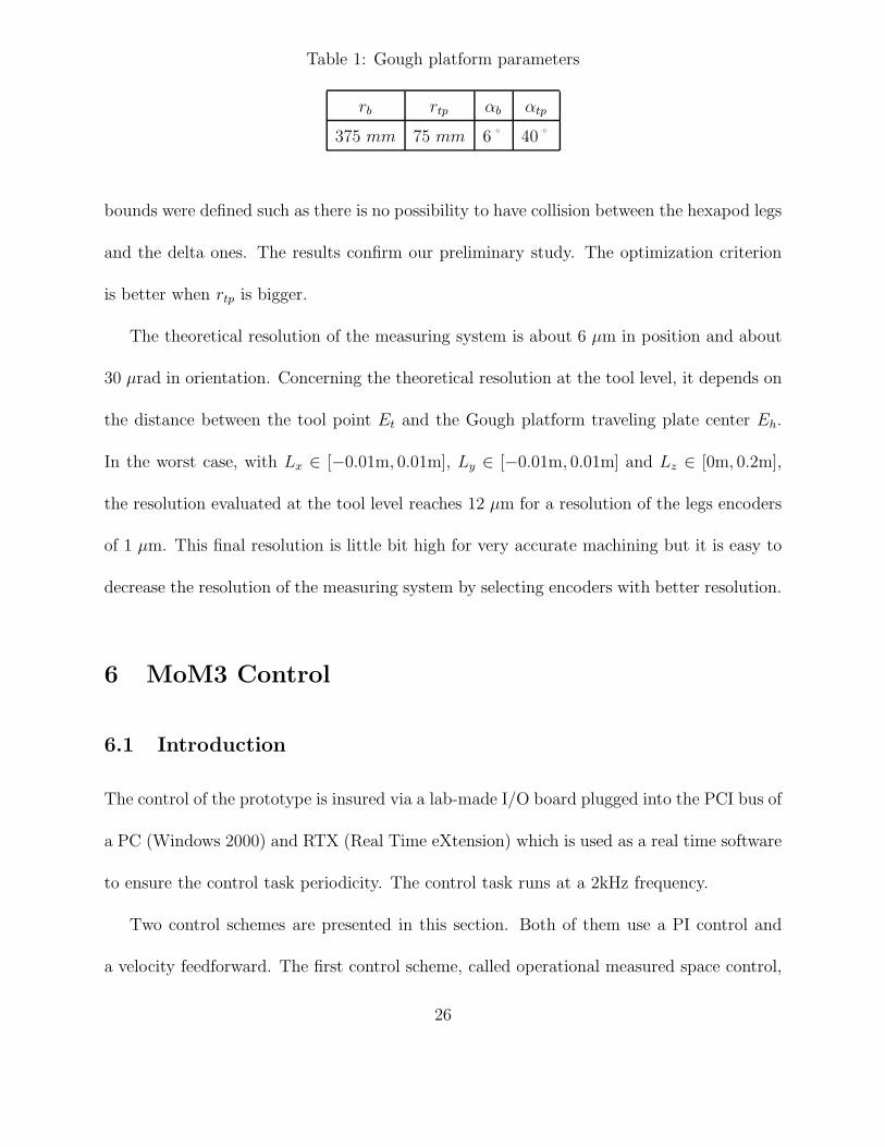
Table 1: Gough platform parameters

rb rtp αb αtp

375 mm 75 mm 6˚ 40˚

bounds were defined such as there is no possibility to have collision between the hexapod legs

and the delta ones. The results confirm our preliminary study. The optimization criterion

is better when rtp is bigger.

The theoretical resolution of the measuring system is about 6 µm in position and about

30 µrad in orientation. Concerning the theoretical resolution at the tool level, it depends on

the distance between the tool point Et and the Gough platform traveling plate center Eh.

In the worst case, with Lx ∈ [−0.01m, 0.01m], Ly ∈ [−0.01m, 0.01m] and Lz ∈ [0m, 0.2m],

the resolution evaluated at the tool level reaches 12 µm for a resolution of the legs encoders

of 1 µm. This final resolution is little bit high for very accurate machining but it is easy to

decrease the resolution of the measuring system by selecting encoders with better resolution.

6 MoM3 Control

6.1 Introduction

The control of the prototype is insured via a lab-made I/O board plugged into the PCI bus of

a PC (Windows 2000) and RTX (Real Time eXtension) which is used as a real time software

to ensure the control task periodicity. The control task runs at a 2kHz frequency.

Two control schemes are presented in this section. Both of them use a PI control and

a velocity feedforward. The first control scheme, called operational measured space control,

26

uses the Gough platform as a “black box” in the feedback loop which gives the TCP pose

(Tool Center Point, equivalent to the end-effector controlled point). In the second control

scheme, called sensor space control, the strut length measurements are directly used for the

feedback. These control schemes are respectively equivalent to the position-based visual

servoing (PBVS) and the image-based visual servoing (IBVS) [24].

6.2 Modeling and notations

Several models, derived in [21], are used in the control schemes: the direct kinematic model-

ing of the Gough platform (DKMGP), the inverse kinematic modeling of the Gough platform

(IKMGP), the Delta robot jacobian matrix Jd and the Gough platform jacobian matrix Jh.

On the control schemes, the matrix Jt represents the matrix which maps a small change

in the length of Gough platform struts to a small displacement of the TCP. Matrices tTh

(respectively hTt) represent the rigid transformation between the TCP frame and the Gough

platform frame (respectively between the Gough platform frame and the TCP frame).

Some notations are used in the control schemes:

• ptdesand ptmes

are the desired and measured position of the TCP,

• xh is the pose of the Gough platform traveling plate,

• l is the vector of the Gough platform strut lengths. ldes represents the vector of the

desired lengths in the case of the sensor space control,

• qd is the Delta joint velocity.

27

Figure 14: Control scheme of MoM3 in operational measured space

6.3 Operational measured space control

In the operational measured space control, the DKMGP appears explicitly (Fig. 14). This

model is calculated with a Newton-Raphson algorithm even though Daney showed that this

method may yield numerical instabilities [25]. However, the orientation of the traveling plate

is very small and there is no singularities in the workspace, so, in this case, the use of the

Newton-Raphson algorithm is acceptable. However, it seems more rigorous to make a control

scheme without the Gough platform DKM. That’s why a sensor space control is proposed.

6.4 Sensor space control

As explained before, sensor space control is equivalent to IBVS when the measuring system

is a camera. In this control scheme (Figure 15), the feedback is made in the sensor space,

here on the Gough platform strut lengths. Then, the matrix Jt transforms the length errors

el in TCP pose errors eptwhich are the inputs of the PI control.

The difficulty of this control scheme is at level of the trajectory generation. Indeed,

as the Delta robot is only a 3-dof mechanism, the parasitical orientation of the traveling

plate cannot be compensated. So, the desired strut lengths ldes cannot be reached since

28

Figure 15: Control scheme of MoM3 in sensor space

they correspond to an unreachable null orientation of the traveling plate. That’s implies el

is never null. To reach eptequal to 0 nevertheless, the matrix Jt must be calculated for

the real pose of the Gough platform. If the matrix Jt is calculated at the desired pose of

the Gough platform an error of about some microns remains. That’s why the pose error of

the Gough platform exhused for the calculation of matrix Jt is estimated. This estimation

allows to cancel the static pose error.

Operational measured space control and sensor space control give similar results but

in order to avoid the possible instabilities of the DKMGP, the second one is used for the

experimentations.

7 Experimental results

7.1 Validation of the measuring system

Before testing the sensor space control, the measuring system must be validated. To do that,

an external measuring system, a laser distancemeter is used. The goal is to show that, when a

29

Figure 16: Experimental set-up for the measuring system validation with end-effector load

load is applied on the actuation chain, the measuring system can measure the displacement

of the end-effector due to the structure deformation. So, the measurement made by the

Gough platform and by the laser distancemeter are compared to see if the Gough platform

is efficient to measure these small displacements.

7.1.1 End-effector perturbation

Figure 16 shows the experimental set-up with an external force applied on the end-effector.

The experimental device is composed of:

• a surface plate with a absolute flatness lower than 1.6 µm,

• a Keyence laser distancemeter with a resolution of 0.2 µm,

• a 80 N to 110 N force generator.

The validation consists in applying a load at the end-effector level and to verify that the

Gough platform detects the Delta mechanism deformation. To do that, the Delta robot is

30

Table 2: Displacement along y axis between a controlled point Pi (i = 1, 2, 3), reached by

the robot without load, and the same point with a 110 N force applied on the end-effector.

Displacement in µm seen by P1 P2 P3

the Delta robot 0.3 1 0.6

the Gough platform 73.7 73.1 70.9

the laser distancemeter 80.4 74.4 76.1

controlled from a classical Cartesian control and moved to a point above the surface plate.

Measurements from the distancemeter and from the Gough platform (using the DKMGP)

are taken and the end-effector pose is calculated from the Delta robot DKM. Then, a 110 N

force is applied on the traveling plate and the displacement detected by the three systems

(the distancemeter, the Gough platform, the Delta robot) are recorded. Table 2 shows the

results for three measurement points.

First of all, the results show the Delta robot control cannot “see” the deformations implied

by the load. The Gough platform detects displacements of about 70 µm when a force is

applied on the end-effector. These measurements are confirmed by the distancemeter. The

measurements made by the Gough platform and the distancemeter are very close and the

little differences can be explained by the resolution of the Gough platform evaluated at about

6 microns.

7.1.2 Delta mechanism frame perturbation

A second validation was made with a load applied on the frame (Figure 17). A 850 N force is

applied on the Delta frame by a person seated on the top of the frame. Then, the procedure

31

is the same than above. Table 3 shows the results for three measurement points.

These results confirm the first ones obtained with the load applied on the end-effector.

The Gough platform is validated on y axis and considering the symmetry of Gough platform,

these results can be extrapolated to z axis and x axis.

Figure 17: Experimental set-up for the measuring system validation with frame load

Table 3: Displacement along y axis between a controlled point Pi (i = 1, 2, 3), reached by

the robot without load, and the same point with a 850 N force applied on the Delta frame

Displacement in µm seen by P1 P2 P3

the Delta robot 1 0.35 1

the Gough platform 70.1 69.2 64.8

the laser distancemeter 65.7 54.8 54.9

32

These results show equally that the Gough platform can detect the Delta frame defor-

mation and thus they can be compensated with control.

7.2 Sensor space control with external force on the end-effector

In this section, the sensor space control is tested. Two different control are compared: the

classical Cartesian Delta mechanism control and the sensor space control. To understand

the interest of SAM, a load is applied on the end-effector and the results obtained with the

two different control strategies are compared (Fig. 18).

To see the influence of the load, the Delta robot is calibrated (details are available in [23]).

Figure 19 shows the results. Sensor space control gives better results (Fig. 19b) than the

classical Cartesian control (Fig. 19a) even if the Delta robot is calibrated. Therefore, thanks

to SAM, the calibration of the actuation chain is no longer necessary. Moreover, it can be

seen from Fig. 19a plots that when the classical Cartesian control is used a 140 N load

doubles the end effector position errors. This does not happen when the sensor space control

is used (Fig. 19b). So SAM allows to maintain the accuracy of the robot whatever the forces

applied on the actuation chain.

Figure 18: 140 N load applied on the MoM3 traveling plate

33

0 20 40 60 80 100 1200

0.05

0.1

0.15

0.2

0.25

Measure number

Pos

ition

err

or (

mm

)

Without loadWith a 140 N load

(a) Classical cartesian control of the calibrated Delta robot

0 20 40 60 80 100 1200

0.05

0.1

0.15

0.2

0.25

Measure number

Pos

ition

err

or (

mm

)

Without loadWith a 140 N load

(b) Sensor space control

Figure 19: Comparison of the classical cartesian control and the sensor space control

34

8 Conclusion

Designing and testing Mom3 has shown the interest of separating Measurement and Actu-

ation when it is applied to parallel mechanisms. In fact, using only well established mech-

anisms (Delta mechanism for the actuation, Gough-platform for measurement), relying on

technologies already in use in precision engineering (magnetic ball joints; linear scale) it has

been possible to propose a system offering the following advantages: (i) the measurement

chain is independent from the process load, (ii) it can compensate for many deformations

encountered in the actuation chain. This has been done thanks to understanding the need of

a number of sensors larger than the actuation dof (while keeping an “iso-measurement” in

our views), optimizing the measurement sub-system so that it can deliver the best resolution

(in a “worst case” point of view) and imagining a control strategy which really takes advan-

tage of the system. Based on such advantages, a designer can create machines whose frame

or mechanism are not machined or assembled with high precision and can even suffer from

permanent deformation. The only requirement would be to guarantee a stiffness suitable for

the process. In some cases, a frame, and even a mechanism with most parts made of wood

can thus be envisioned, as shown in Fig. 20.

9 Acknowledgement

This work has been partially funded by the European project NEXT, “Next Generation of

Production Systems”, Project No. IP 011815.

35

Figure 20: Prototype of MoM3 with a wooden frame and arms

References

[1] Merlet, J.-P., 2006, Parallel Robots, Springer.

[2] Gough, V. E., 1956-1957, “Contribution to discussion of papers on research in automo-

tive stability, control and tyre performance,” Proc. Auto Div. Inst. Mech. Eng., Institute

of mechanical engineering, pp. 392–394.

[3] Clavel, R., Thurneysen, M., Giovanola, J., and Schnyder, M., 2002, “A new 5 dof parallel

kinematics for production applications,” Proc. of the IEEE International Symposium on

Robotics (ISR’02), Stockholm, Sweden, pp. 227–232.

[4] Sheldon, P., 1995, Six axis machine tool, US5388935.

[5] Company, O., Pierrot, F., Launay, F., and Fioroni, C., 2000, “Modelling and preliminary

design issues of a 3-axis parallel machine-tool,” Proc. of the International Conference

on Parallel Kinematic Machines PKM’2000, Ann Arbor, USA, pp. 14–23.

[6] Krause, E. and Co, 2000, Machining system with movable tool head, US6161992.

36

[7] Mooring, B. W., Roth, Z. S., and Driels, M. R., 1991, Fundamentals of Manipulator

Calibration, John Wiley & Sons, Inc., New-York.

[8] Andreff, N., Renaud, P., Martinet, P., and Pierrot, F., 2004, “Vision-based kinematic

calibration of a H4 parallel mechanism: Practical accuracies,” Industrial Robot Inter-

national Journal, 31(3), pp. 273–283.

[9] Tlusty, J., Ziegert, J., and Ridgeway, S., 2000, “A comparison of stiffness characteristics

of serial and parallel machine tools,” Journal of Manufacturing Systems, 2(2), pp. 67–76.

[10] Marquet, F., 2002, Contribution a l’etude de l’apport de la redondance en robotique

parallele, Ph.D. thesis, Universite Montpellier II, Montpellier, France.

[11] Gosselin, C. M. and Zang, D., 2002, “Stiffness analysis of parallel mechanisms using a

lumped model,” International Journal of Robotics and Automation, 17(1), pp. 17–27.

[12] Ecorchard, G. and Maurine, P., 2005, “Self-calibration of delta parallel robots with

elastic deformation compensation,” Proc. of the IEEE International Conference on In-

telligent Robots and Systems (IROS’05), Edmonton, Alberta, Canada, pp. 1283– 1288.

[13] Deblaise, D., Hernot, X., and Maurine, P., 2006, “A systematic analytical method

for pkm stiffness matrix calculation,” Proc. of the IEEE International Conference on

Robotics and Automation (ICRA’06), Orlando, Floride, USA, p. 42134219.

[14] Shirai, Y. and Inoue, H., 1973, “Guiding a robot by visual feedback in assembling tasks,”

Pattern Recognition, 5, pp. 99–106.

37

[15] Dallej, T., Andreff, N., Mezouar, Y., and Martinet, P., 2006, “3D pose visual servoing

relieves parallel robot control from joint sensing,” Proc. of the IEEE International Con-

ference on Intelligent Robots and Systems (IROS’06), Beijing, China, pp. 4291–4296.

[16] David, J., 1989, Machine a Mesurer par Coordonnees, FR2627582.

[17] Hale, L., 1999, Principles and techniques for designing precision machines, Ph.D. thesis,

University of California, Livermore, California, USA.

[18] Slocum, A., 1992, Precision Machine Design, Prentice-Hall, Inc.

[19] Lahousse, L., David, J., Leleu, S., Vailleau, G.-P., and Ducourtieux, S., 2005, “Appli-

cation d’une nouvelle conception d’architecture a une machine de mesure de resolution

nanometrique,” Revue francaise de metrologie, 4(4), pp. 35–43.

[20] Gogu, G., 2005, “Mobility and spatiality of parallel robots revisited via theory of linear

transformations,” European Journal of Mechanics - A/Solids, 24(4), pp. 690–711.

[21] Corbel, D., Company, O., and Pierrot, F., 2008, “Optimal design of a 6-dof parallel

measurement mechanism integrated in a 3-dof parallel machine-tool,” Proc. of the IEEE

International Conference on Intelligent Robots and Systems (IROS’08), Nice, France,

pp. 1970–1976.

[22] Briot, S. and Bonev, I., 2007, “Accuracy analysis of 3-DOF planar parallel robots,”

Mech. Mach. Theory, doi:10.1016/j.mechmachtheory.2007.04.002.

[23] Corbel, D., 2008, Contribution a l’amelioration de la precision des robots paralleles,

Ph.D. thesis, Universite Montpellier II, Montpellier, France.

38

[24] Chaumette, F. and Hutchinson, S., 2006, “Visual servo control, part i: Basic ap-

proaches,” IEEE Robotics and Automation Magazine, 13(4), pp. 82–90.

[25] Daney, D., 1999, “Self calibration of the gough platform using leg mobility constraints,”

10th World Congress on the theory of machine and mechanisms, Oulu, Finland, pp.

104–109.

39