Ensuring Corporate Social and Environmental Responsibility through Vertical Integration and Horizontal Sourcing Adem Orsdemir School of Business Administration, University of California Riverside, Riverside, CA 92521, [email protected]Bin Hu, Vinayak Deshpande Kenan-Flagler Business School, University of North Carolina at Chapel Hill, Chapel Hill, NC 27599, bin [email protected], vinayak deshpande@kenan-flagler.unc.edu Taylor Guitars purchased an ebony mill in Cameroon to ensure corporate social and environmental respon- sibility (CSER) in sourcing, and shared the responsibly-sourced supply of ebony with competitors through horizontal sourcing. Inspired by this case, we investigate vertical integration as an alternative strategy for CSER in sourcing in which a firm can vertically integrate with its supplier in order to ensure responsible practices in the supply chain. In a competitive setting, an exposed CSER violation in one supply chain may increase the competing supply chain’s demand (positive externalities) due to substitution, or decrease the competing supply chain’s demand (negative externalities) due to the public’s suspicion about an industry’s social and environmental practices. Furthermore, NGOs’ scrutiny and reporting policies may influence the likelihood of a violation exposure, as well as demand externalities between the competing supply chains. We examine horizontal sourcing as a potential strategy for mitigating the impact of a CSER externality from a competing supply chain. When horizontal sourcing is infeasible, we find that higher violation exposure externalities better induce CSER, but overly intensive violation scrutiny alongside strongly negative exter- nalities may backfire and impede CSER. By contrast, when horizontal sourcing is feasible, intensive violation scrutiny better induces CSER, but strongly positive externalities may impede industry-wide CSER. These findings have instructive implications for firms pursuing CSER in their supply chain, as well as for NGOs’ violation scrutiny and reporting policies. Key words : responsible sourcing, CSER, NGO, demand externalities 1. Introduction In recent years, several corporate social and environmental responsibility (CSER) violations have come under public scrutiny. Daily Mail (2011) revealed that workers in Nike’s Taiwanese-operated overseas plant were only paid 50 cents per hour, and were mentally and physically abused by their supervisors. Nike had faced similar controversies about their suppliers treating workers poorly since 1
Transcript
Ensuring Corporate Social and Environmental Responsibility
through Vertical Integration and Horizontal Sourcing
Adem OrsdemirSchool of Business Administration, University of California Riverside, Riverside, CA 92521,
sourcing. On the other hand, more positive externalities can better induce responsible sourcing.
Next, we allow the integrated firm to provide responsible supply to the competing firm through
horizontal sourcing, which eliminates risks of violation exposures in both supply chains. With the
possibility of horizontal sourcing, the firms’ behaviors become different. Now NGOs’ more intensive
scrutiny always better induce responsible sourcing, but strongly positive externalities may drive
the integrated firm away from sharing responsible supply, thus impeding industry-wide CSER.
Comparing the two models, we find that in general, the possibility of horizontal sourcing greatly
improves industry-wide CSER.
Our analyses show that NGOs’ scrutiny and reporting policies have a non-straightforward impact
on a firms’ responsible sourcing behavior. NGOs should consciously consider whether their reports
foster positive or negative externalities, and whether horizontal sourcing is feasible in the relevant
industry to avoid unintended consequences. Our findings suggest that when horizontal sourcing is
infeasible, NGOs should refrain from publishing broadly indicting reports that may yield highly
negative externalities, and be cautious about overly intensive scrutiny. On the other hand, with the
possibility of horizontal sourcing, more intensive scrutiny induces better CSER, but NGOs should
refrain from being overly specific in their reports to avoid creating strongly positive externalities,
which discourage the sharing of responsible supply.
A buying firm’s integration with a supplier for CSER often leads to improved pay, added value
and opportunities of economic growth in an underdeveloped region. However, it typically requires
fixed investments and leads to increased sourcing costs for the buying firm. Therefore, it is a priori
unclear whether promoting vertical integration is a viable strategy by which NGOs may stimulate
economic growth in developing nations. Our study shows that despite the costs, vertical integration
for CSER can be economically justifiable for the buying firm, which suggests that NGOs may
indeed promote vertical integration as an approach to improve the livelihood of people in developing
nations.
The rest of this paper is organized as follows. In Section 2 we survey the related literature. The
general model is introduced in Section 3. It is first analyzed without horizontal sourcing in Section
4, then with this option in Section 5, where we also compare the two cases. We next investigate
7
several model extensions in Section 6.1 and confirm the robustness of the base model’s insights,
before concluding our findings in Section 7. The Appendix contains additional results and all proofs.
2. Literature
A relatively new but rapidly growing literature exists on CSER in sourcing. Plambeck and Taylor
(2015) investigate the mechanisms that may incentivize suppliers to comply with responsibility
standards. Chen and Lee (2014) design contracts to screen and identify unethical suppliers. Kim
(2014) studies a manufacturer’s disclosure decision for environmental noncompliance incidences.
Alizamir and Kim (2015) investigate the asymmetric relationship between a supplier and a buyer
in the event of a public disclosure. Xu et al. (2015) analyze policies that may discourage child labor.
Lin (2016) are similarly inspired by Taylor Guitars and investigate co-production in a sustainabil-
ity context. Aral et al. (2014) study the value of third-party sustainability auditing in sourcing
auctions, and conclude that the value of auditing does not necessarily increase for less sustainable
supplier pools. These papers focus on mechanisms to induce CSER in a single decentralized supply
chain. In comparison, we consider CSER in a market with two competitive supply chains. Kraft
et al. (2013a) and Kraft et al. (2013b) investigate the removal of a potentially hazardous substance
from a product in a competitive environment, from the manufacturer’s and NGOs’ perspectives,
respectively. Their models assume that the manufacturer has full control over all aspects of pro-
duction. By contrast, in our model whether to obtain full control of the supply chain is a costly
decision by the manufacturer (through vertical integration). Belavina and Girotra (2014) study the
role of supply network structure in responsible supplier behaviors. Our consideration of vertical
integration is related to supply chain structures, but our model setting is vastly different from
their relational (long-term) sourcing setting. In addition, Belavina and Girotra (2014) consider
supply network structure as an exogenous input, whereas we endogenize the supply chain structure
decision. Chen et al. (2015) study the interaction of whether a firm releases its supplier list with
NGOs’ auditing efforts and suppliers’ compliance efforts, whereas we focus on vertical integration
as an alternative strategy to auditing when the latter is ineffective. Agrawal and Lee (2015) study
how competing manufacturers can use sourcing policies to influence their suppliers’ adoption of
sustainable practices. They implicitly assume that manufacturers can perfectly verify suppliers’
sustainable practices, whereas we focus on situations where this cannot be done unless a supply
chain is vertically integrated. Caro et al. (2015) and Fang and Cho (2015) investigate two new
types of auditing mechanisms, namely joint and shared audits. Particularly, Fang and Cho (2015)
model positive and negative externalities of social responsibility violations similarly to our model.
8
The main difference is that these papers investigate auditing mechanisms, whereas we focus on
situations where audits may be ineffective, and study vertical integration as an alternative strategy,
thus complementing these papers. Guo et al. (2016) study a buyer’s sourcing decision between a
responsible supplier and another supplier who poses potential CSER risks when selling to a socially
conscious market segment. Although this paper has similarities with our work, mainly in that a
firm can choose whether to ensure CSER in sourcing, there are key differences. First, they consider
an isolated supply chain whereas we consider two competing supply chains. Moreover, they assume
a pre-existing responsible supplier, whereas we require vertical integration with a supplier before
a firm can ensure CSER in sourcing. Finally, we consider a vertically integrated firm supplying a
competing firm—a strategy irrelevant in an isolated supply chain.
Our work can be regarded as mitigating CSER violation risks, thus is remotely related to the
literature on strategies to mitigate supply risks. Prominent examples of strategies considered in
this literature include inventory (Tomlin 2006), financial mechanisms (Swinney and Netessine 2009,
Babich 2010, Dong and Tomlin 2012), backup production capability (Yang et al. 2009), diversifica-
tion (Tomlin 2009), and guaranteed delivery contracts (Hu and Kostamis 2015). Our work differs
from this stream of literature in two significant ways. First, in these papers the risks impact the
supply side, whereas in our paper the risk impacts the demand side (due to consumers response to
exposed violations). Second, a key component of our model is the (possibly positive or negative)
externalities of CSER violations, which are absent in the supply risk management setting.
Vertical integration as a strategy has been studied from various perspectives. Perry (1989) pro-
vides a comprehensive review and lists three main drivers of vertical integration: technological
economies, transactional economies, and market imperfections. The first two captures that vertical
integration may lead to various forms of economies of scale. The third one captures that vertical
integration may improve efficiency by eliminating market imperfections such as information asym-
metry. In our paper, we study a new driver of vertical integration, namely that vertical integration
may ensure a firm’s CSER in sourcing. In order to isolate CSER as a new driver, we eliminate the
aforementioned known drivers of vertical integration in our model: we do not assume economies
of scale (in our model vertical integration and ensuring CSER actually causes sourcing costs to
increase) or asymmetric information. Such a model allows us to conclude that CSER, independent
of other known drivers, can drive vertical integration, thus contributing to the vertical integration
literature.
Finally, we discuss the connection and distinction between CSER and product quality manage-
ment. A CSER violation by itself may not involve inferior product quality. For example, a guitar
9
built with illegally sourced wood can have the exact same quality as one built with responsibly-
sourced wood. Therefore, product inspection, a popular tool for quality control, is not applicable
to CSER; the latter requires proper management of the sourcing and production process. On the
other hand, relatively minor quality issues may not have significant social impacts. For example, a
low-quality component’s impact may be limited to increased warranty costs, but does not neces-
sarily raise any concerns about the entire industry. However, serious quality issues, especially when
threatening consumer health and safety, can have significant social impacts, in which case the qual-
ity issue escalates into a CSER violation. A case in point is the 2008 Chinese baby formula scandal,
in which one company’s contaminated products caused 54,000 children to suffer from kidney stones
(Mooney 2008). After the news broke out, consumers avoided all Chinese baby formula brands
(Ramzy 2008). The majority of the product quality management literature does not consider the
social impact of quality issues. For example, Chao et al. (2009) investigate how product recall cost
sharing contracts between suppliers and buyers can induce improved product quality, and Babich
and Tang (2012) explore deferred payment as a means to prevent suppliers from cutting corners. In
comparison, we focus on the social impacts of CSER violations by modeling their (possibly positive
and negative) externalities. To a certain extent, our research sheds light on product quality issues
that are serious enough to have significant social impacts.
3. Model
We model two competing firms selling products in their respective shares of the same market. Each
firm has its own supplier, and the status quo is that neither supply chain is vertically integrated.
We refer to a non-vertically-integrated firm as a buyer. We use A and B to respectively denote the
two supply chains and their members. We assume that currently, each buyer can sell Q units of
its product at a fixed retail price p. Each unit of a buyer’s product requires one unit of a critical
component sourced from its supplier at market wholesale price w. As explained in Section 1, we
aim to study vertical integration as an alternative when conventional approaches, such as auditing,
are ineffective. Accordingly, we assume that a supplier’s compliance with CSER codes cannot be
guaranteed unless a buyer obtains full control of the supplier through vertically integration and
ensures CSER. We denote by σ ∈ (0,1) the probability that a CSER violation will be exposed at
each supplier3, and that the exposure probabilities for the two suppliers are independent (correlated
exposure probabilities are investigated in Section 6.1). This single parameter captures the CSER
risks embedded in this industry’s current common practices. All parties are risk-neutral.
3 There are two sources of uncertainty contributing to a violation exposure: whether a supplier violates CSER codes,and whether the violation gets exposed. Our parameter σ captures their combined effect.
10
If a violation is exposed at one supplier, its buyer’s demand would be negatively affected (see
the examples in Section 1). To be specific, we assume that the demand drops to (1 +α)Q, where
α ∈ (−1,0) captures a violation’s direct demand impact. Furthermore, as we discussed in Section
1, the CSER violation exposure may positively or negatively impact the competing firm’s demand.
Accordingly, we assume that the competing firm’s demand becomes (1 + β)Q, where β ∈ (α,−α).
The assumption that β may be positive or negative captures the possibly positive and negative
externalities of a CSER violation exposure. The assumption of |β|< |α| reflects the intuition that a
violation exposure’s direct impact should be stronger than its indirect impact. Finally, if violations
are exposed at both suppliers, we assume both supply chains’ demands decrease to (1 +α)Q.
We offer two notes about the demand model before moving on. First, we directly assume the
demand changes after a CSER violation exposure instead of modeling consumer behavior which
leads to such demand changes. We do so because the exact market mechanism behind the demand
changes is not our focus, and that a descriptive model is simple yet general enough for us to study
our problem. Such descriptive models are often adopted in the CSER literature (Boyaci and Gallego
2004, Kraft et al. 2013a,b); in particular, Fang and Cho (2015) adopt a setup very similar to ours
to capture externalities of CSER violations. Second, we consider the market size in terms of volume
(demand) for simplicity, while keeping the retail price p fixed—a setting also adopted by Boyaci
and Gallego (2004) and Huang et al. (2015), among others. In practice, firms may adjust their
retail prices to mitigate a violation exposure’s demand impacts. However, even with responsive
pricing, the firms’ revenue changes are likely qualitatively similar to the demand changes in our
model, thus our structural results should not depend on this simplifying assumption.
Of the two buyers, we make the assumption in the main model that only one can ensure CSER
by vertically integrating with its supplier. (In Section 6.5 we investigate the case where both firms
can vertically integrate, and obtain similar insights to those from the main model. We have also
analyzed a model where ensuring CSER is an option after integration, and found that all important
structural results are retained. The analysis is available from the authors.) The assumption that
only one buyer can integrate with its supplier reflects the reality in many industries that vertical
integration requires the buyer to have substantial knowledge about the supplier’s operations and
the environment wherein the supplier resides. For example, Taylor Guitars had had many years of
experience sourcing ebony from Cameroon before purchasing its own mill there (White 2012), and
remained the first and only (as of December 2013) vertically integrated supply chain in the musical
instrument industry (Arnseth 2013). We assume that buyer A incurs a fixed cost f to integrate
with supplier A and ensure CSER. (Along this line, the assumption that buyer B cannot integrate
11
with supplier B can be interpreted as it having a prohibitively high fixed cost for integration.)
Furthermore, consistent with the case of Taylor Guitars, once buyer A integrates with supplier A
and ensures CSER, the component sourcing cost becomes cr > w. This assumption reflects that
suppliers in developing economies often depend on very thin margins which make it economically
infeasible to ensure CSER and improve worker conditions by themselves. The increased sourcing
cost after vertical integration and ensuring CSER reflects the necessary investments and efforts
to rectify irresponsible practices, which often improve the local residents’ livelihood. In Taylor
Guitars’ case, they overcame great difficulties navigating a highly complex legal system to obtain
all required permits, expanded power grid, and doubled worker salaries (White 2012). In exchange,
firm A eliminates its own violation exposure risk (σ = 0). However, even in this case firm A may
still be indirectly affected by an exposed violation at supplier B. This is because consumers may
not be aware of a firm’s CSER efforts, and furthermore may not trust a firm’s CSER claims if a
violation at a similar supplier has just been exposed.
Finally, an integrated firm A may set wholesale price w′ to supply responsibly sourced compo-
nents to buyer B through horizontal sourcing, thus eliminating violation exposure risks at both
supply chains (see Section 1 for relevant examples). In the base model, we assume that buyer B
can choose to source components from either supplier B or firm A, but not both. (In Section 6.4 we
relax this assumption and show that all important structural results are retained.) Since horizontal
sourcing is not ubiquitous in all industries, we first study the model without horizontal sourcing
in Section 4, then with this option in Section 5, which also allows us to compare these two cases.
Buyer A decides whether to integrate
Violation exposure realized
Firm A sets w’
Buyer B decides whether to source from
firm A or supplier B
Production and sales take place
If buyer A integrates and horizontal sourcing possible
Figure 1 Sequence of events in the model.
The general sequence of events is presented in Figure 1. First, buyer A decides whether to ensure
CSER by vertically integrating with supplier A. Next, if horizontal sourcing is feasible, a vertically
12
Symbol Definitionp > 0 Retail pricew> 0 Component wholesale price from a supplierw′ > 0 Endogenous component wholesale price through horizontal sourcingcr >w Unit cost of responsibly sourced componentsf > 0 Fixed cost of vertical integrationQ> 0 Current market size of each firm
α∈ (−1,0) Direct impact of an exposed violationβ ∈ (α,−α) Indirect impact (externalities) of an exposed violationσ ∈ (0,1) Probability of a violation exposure
Table 1 Parameters and Decision Variables
integrated firm A sets wholesale price w′ for buyer B, who decides whether to source from firm A
or supplier B. The random violation exposures are then realized. Before integration, each supplier
has independent probability σ to be exposed of a violation. (The case with correlated violation
exposure risks is investigated in Section 6.1.) Finally, the firms purchase components and make
products to satisfy the demands. Table 1 summarizes all parameters and decision variables.
4. Analysis without horizontal sourcing
We first analyze the model assuming horizontal sourcing is infeasible (i.e., an integrated firm
A cannot supply buyer B). In practice, horizontal sourcing is not ubiquitous for a number of
potential reasons. First, if the component in consideration is highly customized to one firm’s specific
requirements, it will be difficult for another firm to use the same component. Second, firms in
industries where competition is intensive may have psychological resistance to horizontal sourcing.
For example, in recent years, Apple has sought to replace Samsung, a long-time supplier but also
a major competitor in the smart phone and tablet markets, with other suppliers (Luk 2014).
Therefore, it is important to analyze the model without horizontal sourcing. This section’s analysis
also serves as a basis of comparison in Section 5, where we analyze the model with horizontal
sourcing, and highlight the different insights between the two cases.
Our goal is to understand whether the buyer A would integrate with supplier A (and hence
ensure CSER) or stay disintegrated (and hence maintain conventional practices). We use I and
D to respectively denote buyer A’s decision to integrate with supplier A or stay disintegrated.
Therefore, buyer A has two possible strategies, D and I. Let πiX denote buyer i’s expected profit
when buyer A follows strategy X. Below are the expressions of the expected profits (recall that σ
We assume a sufficiently small fixed cost f and a sufficiently small cost of responsibly sourced
component (cr < −[α(p − 2w) + 2(1−√α+ 1
)(p − w)]/α, recall that −1 < α < 0) such that D
does not dominate I. (The specific threshold for f can be found in the Online Supplement.) These
assumptions rule out uninteresting cases; we also know that these assumptions may be satisfied in
practice from the documented examples of vertical integration for CSER such as Taylor Guitars
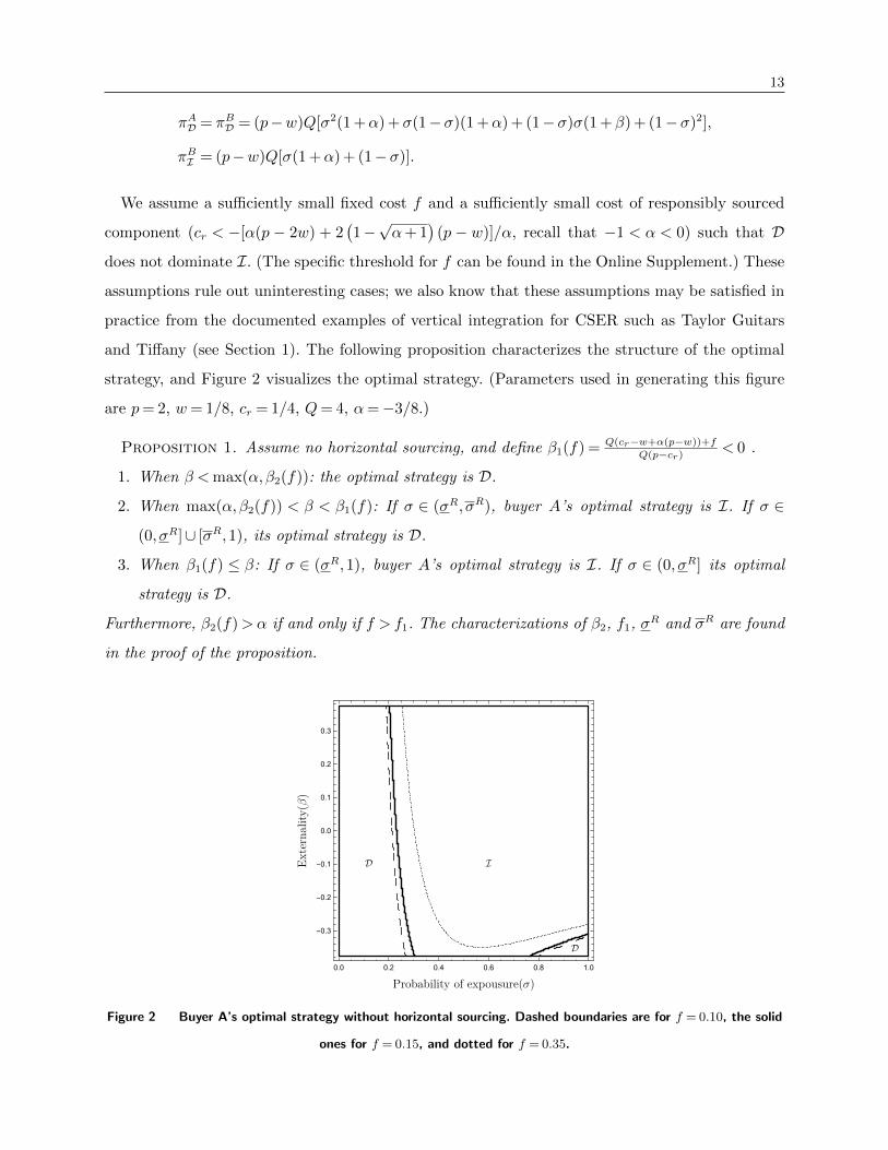
and Tiffany (see Section 1). The following proposition characterizes the structure of the optimal
strategy, and Figure 2 visualizes the optimal strategy. (Parameters used in generating this figure
are p= 2, w= 1/8, cr = 1/4, Q= 4, α=−3/8.)
Proposition 1. Assume no horizontal sourcing, and define β1(f) = Q(cr−w+α(p−w))+f
Q(p−cr)< 0 .
1. When β <max(α,β2(f)): the optimal strategy is D.
2. When max(α,β2(f)) < β < β1(f): If σ ∈ (σR, σR), buyer A’s optimal strategy is I. If σ ∈
(0, σR]∪ [σR,1), its optimal strategy is D.
3. When β1(f) ≤ β: If σ ∈ (σR,1), buyer A’s optimal strategy is I. If σ ∈ (0, σR] its optimal
strategy is D.
Furthermore, β2(f)>α if and only if f > f1. The characterizations of β2, f1, σR and σR are found
in the proof of the proposition.
0.0 0.2 0.4 0.6 0.8 1.0
-0.3
-0.2
-0.1
0.0
0.1
0.2
0.3
Figure 2 Buyer A’s optimal strategy without horizontal sourcing. Dashed boundaries are for f = 0.10, the solid
ones for f = 0.15, and dotted for f = 0.35.
14
Let us understand buyer A’s optimal strategy. One can see that if the violation exposure proba-
bility is sufficiently low, firm A stays disintegrated and maintains conventional practices, which is
intuitive. This observation reflects the basic trade-off between avoiding one’s own violation expo-
sures, and reducing sourcing costs. What is less intuitive is that, with strongly negative exposure
externalities, high probabilities of violation exposure can also drive firm A to stay disintegrated
and maintain conventional practices rather than to become vertically integrated and ensure CSER.
The cause of this behavior is the negative externalities. While an integrated firm A can eliminate
its own violation risks through vertical integration, it is still vulnerable to negative externalities if
a violation is exposed at supplier B. When externalities are strongly negative, and exposure prob-
abilities are high, firm A’s own CSER efforts become futile as its demand is likely to be negatively
impacted by an exposed violation at the other firm anyway. As a result, firm A chooses to remain
disintegrated instead.
The above observations have managerial implications for NGOs focusing on CSER. They can
influence the violation exposure probabilities to some extent by adjusting the resources dedicated
to scrutinizing firms, and it is easy to assume that more intensive scrutiny is more likely to “scare”
firms into ensuring CSER in sourcing (Baron et al. 2011, Greenhouse 2013). Nevertheless, our
analysis suggests that in scenarios where externalities are strongly negative, such NGOs’ scrutiny
efforts may backfire and drive firms away from CSER.
On the other hand, note that the I region grows as the externalities become more positive. This
observation is formalized in the following proposition.
Proposition 2. Assume no horizontal sourcing. The range of probabilities of exposure σ where
buyer A’s optimal strategy is I grows as externality β increases.
Recall our discussion in Section 1 that NGOs can influence exposure externalities by choosing
how they report violations: a report can broadly indict an industry or a region and foster negative
externalities, or be more specific about firms directly involved in a violation while exonerating
uninvolved firms and foster positive externalities. Proposition 2 suggests that, without horizontal
sourcing, higher externalities may be more in line with inducing CSER. (Interestingly, if horizontal
sourcing is feasible, this is no longer the case; see Section 5.)
So far we have discussed the CSER behaviors. Next we investigate the firms’ profits. One might
intuitively think that for buyer B, who sources from a conventional supplier and faces direct viola-
tion exposure risks, an increase in the exposure probability would decrease its profit. Interestingly,
this is not always true, as presented in the next proposition.
15
Proposition 3. Assume β < 0, and buyer A’s optimal strategy is D, then increasing σ by τ ∈
(τ c, τ c) shifts the optimal strategy to I and increases buyer B’s profit. The characterizations of ∆1,
τ c and τ c are found in the proof of the proposition.
With negative exposure externalities, buyer B may actually benefit from an increased probability
of a violation exposure, because when it pushes firm A into vertical integration, buyer B will be
free of any negative externalities due to firm A’s violations.
To summarize, without horizontal sourcing, our analysis of the model suggests that the external-
ities of exposed CSER violations significantly influence firms’ behaviors. In general, a firm is more
likely to ensure CSER through vertical integration with higher externalities, but when externalities
are strongly negative, overly intensive scrutiny may backfire and drive a firm away from CSER.
These findings provide instructive implications for NGOs to strategically influence the externalities
and violation exposure probabilities to induce CSER in sourcing.
5. Analysis with horizontal sourcing
In this section, we analyze the model with horizontal sourcing. We continue to use the notations
from Section 4, where D and I respectively represent buyer A’s strategy of staying disintegrated
and maintaining conventional practices, and integrating with supplier A and ensuring CSER. Addi-
tionally, we use subscripts S and N on I to respectively denote whether or not buyer B sources
from the integrated firm A through horizontal sourcing. We denote by w′ the horizontal sourcing
wholesale price set by an integrated firm A. Using backward induction, we solve the three-stage
(integration, pricing, procurement) sequential game (as shown in Figure 1). The following propo-
sition characterizes the equilibrium.
Proposition 4. Assume horizontal sourcing is feasible. There exists a threshold 0 ≤ β3(f) <
w−cr−α(p−w)
p−cr such that
1. When β ≤ β3(f): If σ ∈ (0, σ1], the equilibrium is D. If σ ∈ (σ1,1), it is IS.
2. When β3(f)<β < w−cr−α(p−w)
p−cr : If σ ∈ (0, σR], the equilibrium is D. If σ ∈ (σR, σ2], it is IN . If
σ ∈ (σ2,1), it is IS.
3. When w−cr−α(p−w)
p−cr ≤ β: If σ ∈ (0, σR], the equilibrium is D. If σ ∈ (σR,1), it is IN .
The equilibrium horizontal sourcing wholesale price is w′ =w+ασ(w−p). The threshold β3(f) is a
continuous increasing function of f characterized in the proof of the proposition. The characteriza-
tion of σR is found Proposition 1, and those of σ1 and σ2 are found in the proof of the proposition.
16
0.0 0.2 0.4 0.6 0.8 1.0
-0.3
-0.2
-0.1
0.0
0.1
0.2
0.3
Figure 3 Firms’ equilibrium strategy with horizontal sourcing. Dashed boundaries are for f = 0.10, the solid
ones for f = 0.15, and dotted for f = 0.35.
Figure 3 illustrates the equilibria generated with the same parameters as in Figure 2. An imme-
diate observation about Figure 3 is that higher violation exposure probabilities drive firm A into
vertical integration and CSER. This is in stark contrast to Proposition 1 and Figure 2 (the case
without horizontal sourcing), where higher exposure probabilities may drive firm A away from
CSER. As we explained in Section 4, when horizontal sourcing is infeasible, scrutiny may discour-
age firm A’s CSER efforts because the negative externalities of buyer B’s violation exposures may
make the efforts futile. When horizontal sourcing is feasible, however, firm A can eliminate nega-
tive externalities by sharing responsible supply with buyer B, thus scrutiny always drives CSER.
Furthermore, when firm A is integrated and ensures CSER (in the I regions), higher exposure
probabilities drive firm A to share responsible supply with buyer B (equilibrium shifting from INto IS), expanding CSER to the entire industry. This is because under more intensive scrutiny,
buyer B is willing to pay more premium for responsible supply, strengthening the incentive for
firm A to share it.
We then investigate the impact of externalities. Interestingly, higher externalities cause the D
and IN regions to grow against the IS region; this can be observed in Figure 3, and we provide an
analytical characterization as well:
Proposition 5. Assume that horizontal sourcing is feasible, then the range of violation exposure
probabilities σ where IS is the equilibrium shrinks as externality β increases.
In addition, once again in stark contrast to Proposition 2 and Figure 2, strongly positive exter-
nalities actually impair industry-wide CSER in sourcing: Proposition 5 and Figure 3 show that
17
within the I regions where firm A is integrated and ensures CSER, when externalities are strongly
positive, firm A stops sharing responsible supply with buyer B (equilibrium shifting form IS to IN).
The explanation is that, positive externalities mean that firm A benefits from buyer B’s violation
exposures, which is a disincentive for the former to share responsible supply with the latter. Note
that this issue is nonexistent without horizontal sourcing. Therefore, interestingly, while horizontal
sourcing resolves the complication that hinders the effectiveness of scrutiny, it creates a new com-
plication in externalities’ impacts on industry-wide CSER. These observations suggest that NGOs
should consciously consider whether horizontal sourcing is feasible in the relevant industries when
choosing their scrutiny and reporting policies, so as to avoid unintended consequences.
Next we investigate the firms’ profits. Interestingly, we find that both firms may benefit from
more intensive scrutiny.
Proposition 6. Assume β < 0 and σ1−∆2 <σ≤ σ1 so that the equilibrium is D, then increas-
ing σ by τ ∈ [τ r, τ r] shifts the equilibrium to IS and increases both firm A and buyer B’s profits.
The characterizations of ∆2, τ r and τ r are found in the proof of the proposition.
Actually, in the case presented in Proposition 6, not only do both firms earn more profits, the
industry is also transformed from fully conventional to fully responsible. Therefore, the society also
benefits in terms of CSER, making this a win-win-win situation.
As a final note, we compare the CSER outcomes when horizontal sourcing is infeasible (Section 4)
with those when horizontal sourcing is feasible (Section 5), to appraise the CSER value of horizontal
sourcing. Because horizontal sourcing is an additional lever that benefits the social responsibility
outcome, the possibility of horizontal sourcing strictly improves CSER:
Proposition 7. I ⊂ {IN⋃IS}.
Moreover, when one compares Figures 2 and 3, it is apparent that horizontal sourcing brings CSER
to the entire industry in a significant parameter region. Thus, horizontal sourcing greatly improves
industry-wide CSER.
To summarize, when horizontal sourcing is feasible, intensive scrutiny drives CSER, but strongly
positive externalities may backfire and discourage an integrated firm from sharing responsible sup-
ply with competitors. These observations contrast starkly with those in Section 4 when horizontal
sourcing is infeasible, where higher externalities provide the right incentives, but overly intensive
scrutiny may backfire. In general, the possibility of horizontal sourcing greatly improves CSER.
18
6. Extensions
Thus far we have adopted a base model which allowed us to derive structural properties and reveal
insights. It is important to verify that the key insights are not driven by specific assumptions in
the base model. In this section we investigate various extensions of the base model and show that
the key insights remain unchanged, and in some cases also make new observations pertaining to
the extensions.
6.1. Correlated violation exposure risks
In the base model we have assumed independent violation exposure probabilities for the two sup-
pliers. In practice, they may be correlated to some extent, either positively or negatively. A case
of a positive correlation may be that an exposed violation at one supplier triggers more intensive
scrutiny of other similar suppliers. On the other hand, observing an exposed violation at one sup-
plier, other suppliers may take proactive measures to rectify and/or conceal malpractices, leading
to negatively correlated violation exposure risks. In this section, we investigate our model with
correlated violation exposure probabilities. We carry out the investigation by means of a numerical
study as outlined below.
Recall that in the main model, we assume that each supplier faces an independent violation
exposure probability σ. To introduce correlations without changing the marginal probabilities
(namely each supplier still has probability σ to be exposed of a violation), we adopt the correlated
bi-variant Bernoulli model in Hu and Kostamis (2015) as described below. We denote the joint
probabilities of four possible exposure scenarios by q00, q01, q10 and q11, where 1 represents a
violation exposure and 0 represents no exposure, at suppliers A and B. For example, q10 represents
the probability of a violation exposure at supplier A but not at supplier B. Using a parameter
r ∈ [−1,1] to indicate correlation, we define (q00, q01, q10, q11) = (rσ(1− σ) + (1− σ)2, (1− r)σ(1−
σ), (1−r)σ(1−σ), r(1−σ)σ+σ2) for r≥ 0, and (q00, q01, q10, q11) = (rσ2 +(1−σ)2, σ−(r+1)σ2, σ−
(r + 1)σ2, (r + 1)σ2) for r < 0. As r is increased from −1 to 0 to 1, the two suppliers’ violation
exposure risks change from never occurring simultaneously (q11 = 0) to being independent to always
occurring simultaneously (q01 = q10 = 0).
Figures 4 and 5 depict buyer A’s optimal strategies when horizontal sourcing is infeasible and
feasible, respectively, for representative values of r. The other parameters are p = 2, w = 1/8,
cr = 1/4, Q= 4, α=−3/8, and f = 0.1, as in all previous figures. Case (a)’s of Figures 4 and 5 have
positive correlations, and are structurally similar to Figure 2 and Figure 3, thus confirming that
the main insights in Section 4 and 5 continue to hold with positively correlated violation exposure
risks. Case (b)’s of Figures 4 and 5 have negative correlations. In Figure 4, Case (b) does not share
19
similar structures as the D region in the lower-right corner of Figure 2 does not exist in the lower
panel of Figure 4. However, we note that Case (b)’s do not cover the entire range of exposure
probabilities, but are limited to σ . 0.53. This is because high exposure probabilities cannot be
negatively correlated. For example, if each of suppliers A and B has marginal probability 0.9 of a
violation exposure, then they will almost always be exposed of violations simultaneously, thus must
be strongly positively correlated. Therefore, (b) of Figure 4 and 5 is not completely comparable to
Figure 2 and Figure 3; and where comparable (σ. 0.53), they are structurally similar.
0.0 0.2 0.4 0.6 0.8 1.0
-0.3
-0.2
-0.1
0.0
0.1
0.2
0.3
(a) r= 0.2 and r= 0.4
0.0 0.1 0.2 0.3 0.4 0.5
-0.3
-0.2
-0.1
0.0
0.1
0.2
0.3
(b) r= −0.4 and r= −0.2
Figure 4 Buyer A’s optimal strategy with correlated violation exposure probabilities, no horizontal sourcing.
The solid (dotted) boundaries are for r= 0.2 and r= −0.4 (r= 0.4 and r= −0.2)
An interesting question that would have important managerial implications is how CSER out-
comes change with the correlation between violation exposure risks. We find that with positive
externalities, the integration regions where buyer A integrates with supplier A (I/IS/IN) grow
when the correlation increases (algebraically, rather than in absolute magnitude); and with neg-
ative externalities, the integration regions shrink when the correlation increases. The intuition is
as follows. A higher correlation means that the world is less likely to be in the state where only
one of the two suppliers is exposed of a violation. Consequently, a disintegrated buyer A is less
likely to experience violation exposure externalities. Therefore, with positive (negative) externali-
ties, higher correlation makes conventional practices less (more) attractive, causing the integration
regions to grow (shrink). The above insight may be instructive for NGOs in choosing their scrutiny
20
0.0 0.2 0.4 0.6 0.8 1.0
-0.3
-0.2
-0.1
0.0
0.1
0.2
0.3
(a) r= 0.2 and r= 0.4
0.1 0.2 0.3 0.4 0.5 0.6
-0.3
-0.2
-0.1
0.0
0.1
0.2
0.3
(b) r= −0.4 and r= −0.2
Figure 5 Firms’ equilibrium strategies with correlated violation exposure probabilities, with horizontal sourcing.
The solid (dotted) boundaries are for r= 0.2 and r= −0.4 (r= 0.4 and r= −0.2)
policies. NGOs may influence violation exposure correlations to some extent. For example, when
a violation is exposed, NGOs can focus resources on the involved supplier, reducing correlations,
or allocate more resources to other similar suppliers, increasing correlations. Our results suggest
that NGOs should consider the nature of externalities in the relevant industry, and foster higher
(lower) correlations with positive (negative) externalities.
6.2. Non-exclusive suppliers
In the main model we assumed that each buyer has its exclusive supplier. In this section, we extend
the base model to allow buyers to choose one of two available suppliers, and thus, they may end up
sourcing from a shared supplier. In particular, for both no horizontal and horizontal sourcing cases,
we assume that if buyer A decides to stay disintegrated, then the buyers simultaneously choose the
supplier to source from (either supplier A or B). In this case, if the buyers choose to source from
a shared supplier, a violation exposure at this supplier affects both buyers’ demands at the same
time (i.e. demands drop to (1 +α)Q). We denote the equilibrium of both buyers sharing a supplier
with DC , and that of the buyers sourcing from different suppliers with DU . We first present the
case without horizontal sourcing in Proposition 8 and Figure 6. The figure is generated using the
same parameters as in Figure 2 and f = 0.1.
Proposition 8. Assume no horizontal sourcing.
1. When β ≤ β1(f): The optimal strategy is D.
21
2. When β1(f)<β < 0: If σ ∈ (0, σ3], the equilibrium is DC. Otherwise, if σ ∈ (σ3,1), it is I.
3. When 0≤ β: If σ ∈ (0, σR], the equilibrium is DU . If σ ∈ (σR,1), it is I.
The threshold σ3 is a continuous decreasing function of β and its characterization is found in the
proof of the proposition. The characterizations of σR and β1(f) are found in Proposition 1.
0.0 0.2 0.4 0.6 0.8 1.0
-0.3
-0.2
-0.1
0.0
0.1
0.2
0.3
Figure 6 Equilibria with non-exclusive suppliers without horizontal sourcing.
Note that when externality is nonnegative, all the equilibria are the same as in the base model
since the buyers source from different suppliers. However, with negative externalities, the buyers’
sourcing behaviors change compared to the base model because they source from a shared supplier.
Consequently, the region where buyer A stays disintegrated for high probabilities of exposure
in Proposition 1 (the D region in the lower right corner of Figure 2) disappears. The reason
is that with strong negative externalities buyer A benefits more from sharing a supplier with
buyer B and avoiding the externality than from integrating with its supplier and facing strong
negative externalities. Thus, when we allow non-exclusive suppliers, higher probabilities of exposure
always drive CSER. As for the impact of externality on the equilibrium structure, Proposition 8
implies that higher externalities always drive CSER. This trend is unchanged from the base model
(Proposition 2).
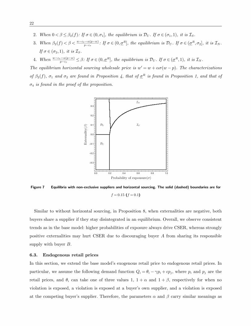
Next, we present and illustrate the case with horizontal sourcing. Figure 7 uses the same param-
eters as Figure 2 and f = 0.1.
Proposition 9. Assume horizontal sourcing is feasible, and define σ4 = 2Q(cr−w)+f
2αQ(w−p) .
1. When β ≤ 0: If σ ∈ (0, σ4], the equilibrium is DC. If σ ∈ (σ4,1), it is IS.
22
2. When 0<β ≤ β2(f): If σ ∈ (0, σ1], the equilibrium is DU . If σ ∈ (σ1,1), it is IS.
3. When β2(f)< β < w−cr−α(p−w)
p−cr : If σ ∈ (0, σR], the equilibrium is DU . If σ ∈ (σR, σ2], it is IN .
If σ ∈ (σ2,1), it is IS.
4. When w−cr−α(p−w)
p−cr ≤ β: If σ ∈ (0, σR], the equilibrium is DU . If σ ∈ (σR,1), it is IN .
The equilibrium horizontal sourcing wholesale price is w′ = w+ασ(w− p). The characterizations
of β2(f), σ1 and σ2 are found in Proposition 4, that of σR is found in Proposition 1, and that of
σ4 is found in the proof of the proposition.
0.0 0.2 0.4 0.6 0.8 1.0
-0.3
-0.2
-0.1
0.0
0.1
0.2
0.3
Figure 7 Equilibria with non-exclusive suppliers and horizontal sourcing. The solid (dashed) boundaries are for
f = 0.15 (f = 0.1)
Similar to without horizontal sourcing, in Proposition 8, when externalities are negative, both
buyers share a supplier if they stay disintegrated in an equilibrium. Overall, we observe consistent
trends as in the base model: higher probabilities of exposure always drive CSER, whereas strongly
positive externalities may hurt CSER due to discouraging buyer A from sharing its responsible
supply with buyer B.
6.3. Endogenous retail prices
In this section, we extend the base model’s exogenous retail price to endogenous retail prices. In
particular, we assume the following demand function Qi = θi− γpi + εpj, where pi and pj are the
retail prices, and θi can take one of three values 1, 1 + α and 1 + β, respectively for when no
violation is exposed, a violation is exposed at a buyer’s own supplier, and a violation is exposed
at the competing buyer’s supplier. Therefore, the parameters α and β carry similar meanings as
23
in the base model. The parameters γ and ε measure a product’s demand sensitivities to its own
price and the competing product’s price. Due to this model’s complexity, we resort to numerical
studies. We focus on the non-trivial cases where both buyers’ outputs are positive, and consistently
observe that the model behaves qualitatively similar to our base model. This is evident in the
representative examples (for both no horizontal sourcing and with horizontal sourcing) we provide
in Figure 8, which are generated with parameters α=−3/8, w = 1/8, cr = 1/4, γ = 0.6, f = 0.1,
and ε= 0.1.
0.0 0.2 0.4 0.6 0.8 1.0
-0.3
-0.2
-0.1
0.0
0.1
0.2
0.3
(a) No horizontal sourcing
0.0 0.2 0.4 0.6 0.8 1.0
-0.3
-0.2
-0.1
0.0
0.1
0.2
0.3
(b) With horizontal sourcing
Figure 8 Equilibria with endogenous retail prices. The solid (dashed) boundaries are for f = 0.015 (f = 0.01)
6.4. Capacitated horizontal sourcing
In this section, we consider a scenario in which the integrated firm A has enough capacity C for
itself, but not enough to also provide all the needed supply for buyer B through horizontal sourcing,
namely Q < C < 2Q. In this case, we assume that in equilibrium IS, buyer B purchases C −Q
units of (responsible) supply from firm A and the rest 2Q−C units from (conventional) supplier
B to fulfill demand Q. In other words, buyer B dual-sources from responsible and conventional
sources in equilibrium IS. Recall that a violation may be exposed at the conventional supplier B
with probability σ, which still supplies buyer B (even though only partially), thus buyer B faces
the same violation exposure probability σ in equilibrium IS. However, the demand impacts of such
a violation exposure may be lower because only a portion of buyer B’s products are involved. To
model this effect, we define direct and indirect proportional demand impact parameters respectively
24
as αs = (2Q−C)α/Q, βs = (2Q−C)β/Q. We also define k=C −Q as firm A’s capacity in excess
of its own demand that can be sold to buyer B. Proposition 10 characterizes the equilibria of this
model extension.
Proposition 10. Assume horizontal sourcing is feasible and f < f2. There exist thresholds
β4(f) and k1(f,β) satisfying β(f)<β4(f)<β(f)< 0 and k(β, f)<k1(f,β)<k(β, f), such that
1. When β < β4(f) and k < k1(f,β): If σ ∈ (0, σ5]∪ [σ6,1), the equilibrium is D. If σ ∈ (σ5, σ6),
it is IS.
2. When β4(f)≤ β ≤ β3(f), or β < β4(f) and k≥ k1(f,β): If σ ∈ (0, σ5], the equilibrium is D. If
σ ∈ (σ5,1), it is IS.
3. When β3(f)<β < w−cr−α(p−w)
p−cr : If σ ∈ (0, σR], the equilibrium is D. If σ ∈ (σR, σ2], it is IN . If
σ ∈ (σ2,1), it is IS.
4. When w−cr−α(p−w)
p−cr ≤ β: If σ ∈ (0, σR], the equilibrium is D. If σ ∈ (σR,1), it is IN .
The equilibrium horizontal sourcing wholesale price is w′ = w+ασ(w− p). The characterizations
of β2(f) and σ2 are found in Proposition 4, that of σR is found in Proposition 1, and those of σ5,
σ6, β, β, k and k are found in the proof of the proposition.
0.0 0.2 0.4 0.6 0.8 1.0
-0.3
-0.2
-0.1
0.0
0.1
0.2
0.3
(a) C = 4.1
0.0 0.2 0.4 0.6 0.8 1.0
-0.3
-0.2
-0.1
0.0
0.1
0.2
0.3
(b) C = 7.9
Figure 9 Equilibrium when firm A’s capacity is less than the total demand, i.e., C < 2Q
Figure 9, generated with the same parameters as before (i.e., p= 2, w = 1/8, cr = 1/4, Q= 4,
f = 0.1), illustrates Proposition 10 with low and high capacities. When an integrated firm A’s
capacity is low, horizontal sourcing does not substantially reduce buyer B’s violation exposure
25
risks. As a result, the equilibrium structure of Figure 9(a) resembles that of Figure 2 in Section
4 without horizontal sourcing. On the other hand, when an integrated firm A’s capacity is high
enough to meaningfully reduce buyer B’s violation exposure risks through horizontal sourcing,
the equilibrium structure of Figure 9(b) resembles that of Figure 3 in Section 5 with horizontal
sourcing. This trend is expected, and confirms that our insights are useful in understanding the
impact of horizontal sourcing even with limited capacities.
6.5. Both buyers can vertically integrate
In this extension we allow both buyers to vertically integrate and ensure CSER. (This is equivalent
to assuming that both buyers have low fixed costs for vertical integration.) Let tuple (k; l) denotes
that buyer A plays strategy k and buyer B plays strategy l; e.g., (I;D) denotes that only buyer
A is vertically integrated. When both buyers can vertically integrate and ensure CSER, horizontal
sourcing becomes unnecessary. Therefore, we do not consider horizontal sourcing in this extension.
Proposition 11. Assume both firms can vertically integrate and no horizontal sourcing.
1. When β ≤max(α,β2(f)): the optimal strategy is D.
2. When max(α,β2(f))β < β1(f): If σ ∈ (σR, σR), (I,I) is an equilibrium. If σ ∈ (0, σR]∪ [σR,1),
(D,D) is an equilibrium.
3. When β1(f)≤ β ≤ 0: If σ ∈ (σR,1), (I,I) is an equilibrium. If σ ∈ (0, σR], (D,D) is an equi-
librium.
4. When 0< β: If σ ∈ (σ7,1), (I,I) is an equilibrium. If σ ∈ (σR, σ7], either (I,D) or (D,I) is
an equilibrium. If σ ∈ (0, σR], (D,D) is an equilibrium.
Furthermore, β2(f)>α if and only if f > f1. The characterizations of σR, σR, β1 and β2 are found
in Proposition 1 and that of σ7 is found in the proof of the proposition.
One can see that Proposition 11 where both buyers can vertically integrate is very similar to
Proposition 1 where only buyer A can vertically integrate. In addition, the base model’s property
that higher externalities drive vertical integration and thus CSER (Proposition 2) also carries over:
Proposition 12. In the equilibrium described in Proposition 11, the range of σ where at least
one firm plays the strategy I grows as β increases.
In summary, all main results in Section 4 where only buyer A can vertically integrate carry over
to this extension where both buyers can vertically integrate.
26
7. Conclusion
In an increasingly socially- and environmentally-conscious world, when a supplier’s CSER violation
is exposed, its client often suffers market consequences. In addition, competing firms may benefit
from the exposure due to substitution, or suffer from it due to consumer suspicion about general
practices in the industry. The rapid globalization makes managing CSER in sourcing ever more
challenging, and in some cases conventional approaches such as auditing may be ineffective.
On the other hand, many NGOs attempt to promote CSER through the combined power of
media and markets by exposing violations to socially- and environmentally-conscious consumers.
In this process, they can choose the resources allocated to scrutinizing suppliers, as well as the
way violations are publicized. The former choice affects the likelihood of a violation being exposed,
whereas the latter choice influences whether an exposed violation benefits or hurts other compet-
ing firms. The complex interactions make it non-straightforward for NGOs in determining what
violation scrutiny and reporting policies best induce CSER in the industry.
Inspired by the case of Taylor Guitars, we investigated vertical integration as an alternative
strategy for CSER in sourcing when conventional approaches such as auditing are ineffective,
and the impact of horizontal sourcing on the strategy. We modeled two competing firms, one
of which may vertically integrate with its supplier which ensures CSER. An exposed violation
impacts the demand of the involved firm, but may also positively or negatively impact that of the
competing firm. We first investigated the model assuming horizontal sourcing is infeasible, then
allow horizontal sourcing through which a vertically integrated firm can supply the other buyer,
and compare the results.
Our findings indicate that firms’ optimal/equilibrium integration and CSER decisions are non-
trivial, and differ with and without horizontal sourcing. We first show that vertical integration can
be a viable strategy for CSER in sourcing, hence identifying a new driver of vertical integration—
corporate social and environmental responsibility considerations. We then analyze whether hor-
izontal sourcing can be an effective strategy to mitigate CSER externalities from a competing
supply chain. Our analysis shows that firms’ behaviors differ based on whether horizontal sourcing
is feasible. When horizontal sourcing is infeasible, higher violation exposure externalities improve
CSER, but overly intensive violation scrutiny alongside strongly negative externalities may backfire
and discourage CSER. When horizontal sourcing is feasible, however, these trends are inverted:
intensive violation scrutiny improves CSER, but strongly positive externalities may discourage an
integrated firm from sharing responsible supply with competitors, impairing industry-wide CSER.
In general, horizontal sourcing can greatly improve CSER in an industry. These findings have
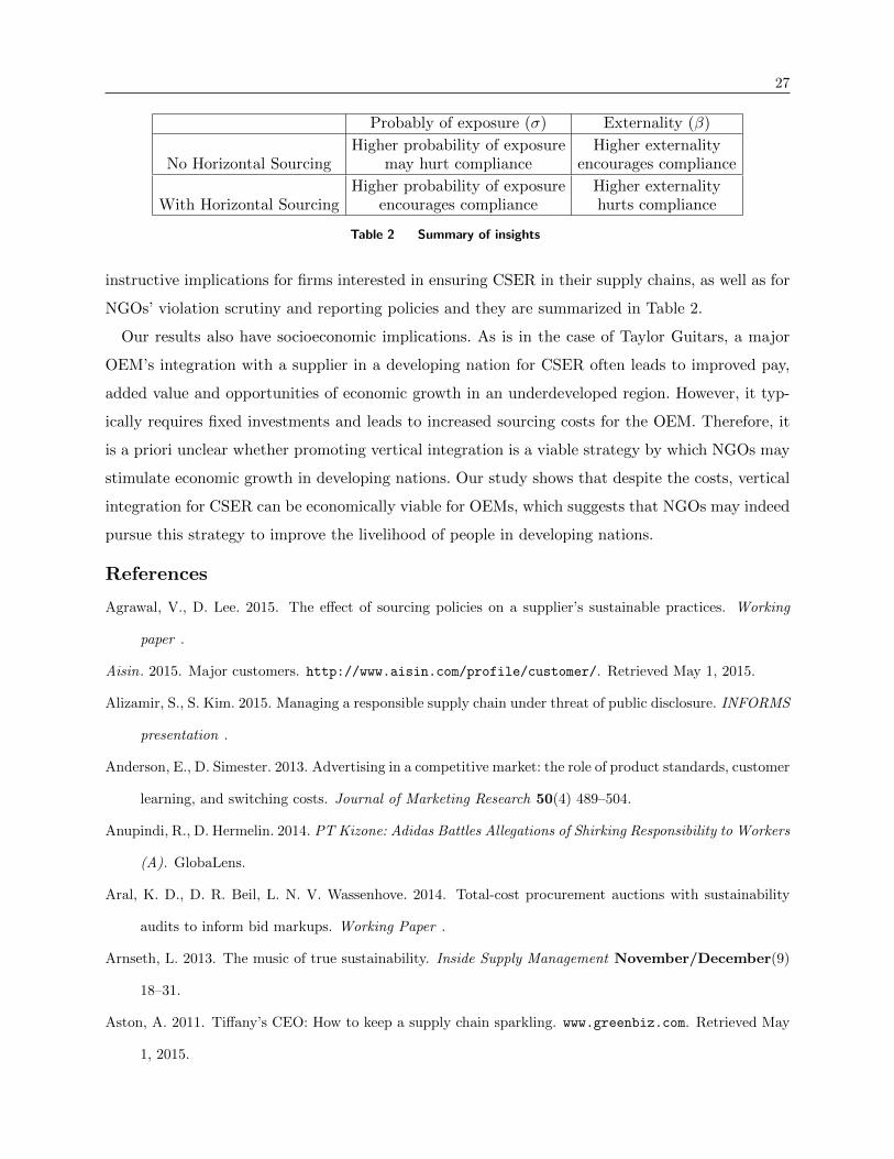
27
Probably of exposure (σ) Externality (β)
No Horizontal SourcingHigher probability of exposure
may hurt complianceHigher externality
encourages compliance
With Horizontal SourcingHigher probability of exposure


![[Shiseido’s Corporate Social Responsibility] · Shiseido's Corporate Social Responsibility Back Issues 2010 [Shiseido’s Corporate Social Responsibility] "Beautiful Society, Bright](https://static.documents.pub/doc/80x56/5f170ccfbe73e76f437bb14c/shiseidoas-corporate-social-responsibility-shiseidos-corporate-social-responsibility.jpg)


