Entanglement and Non Local Correlations

Entanglement and Non Local Correlations:

Quantum Resources for Information Processing

Ph.D. Thesis

Ph.D. Candidate:

Giuseppe Prettico

Thesis Supervisor:

Dr. Antonio Acın

ICFO - Institut de Ciences Fotoniques

2

A zia Rita e zio Mimino, per averci insegnatoche l’umilta e la semplicita possono rendere

immortale l’essere umano.

4

Acknowledgements

This work represents a great achievement of my life that could not havebeen possible without the help of many of you. I believe it is fundamentalto start with the person who offered me the chance of a PhD in his groupfive years ago. Muchisima gracias Toni! Beloved boss, available person, andfun friend. Thank you for the amount of patience you have had in theseyears with me, for the interesting Physics I’ve learnt with you... for havingshowed me that success and modesty can coexists only in special people.

Special thanks go to my collaborators, Dani, Remik, Junu, Chirag andGonzalo with which I learnt many interesting aspects of the Quantum In-formation World.

A big thank goes also to the whole QIT group which I’ve seen chang-ing and expanding in these years: Ale, Stefano, Artur, Dani, Mafi, Mario(Leandro), Augusto, Planeta, Chirag, Jonatan, Anthony, Tobias, Gonzalo,Rodrigo, Lars, Belen, Elsa, Ariel ...

Thank you for all kind of interesting discussions we had...I guess inthe future will be very hard to have colleagues so open-minded like you. Iwant to add that I’ll never forget the nice conferences, barbecues, and otherevents that we have enjoyed together in these years. Thanks.

Thanks to the HR and KTT staff of Icfo for the intense work thatthey do to give us a better life (without boring bureaucracy, through niceevents...) in particular to Mery and Marta.

It is a pleasure to say thank you to the people at the Dipartimento diEnergetica in Rome, in particular to A. Belardini and F. Michelotti whichgave me through their teachings a great stimulus to start a PhD programme.

5

Per terminare, vorrei ringraziare i miei genitori per essere stati un sup-porto fondamentale in questi anni... nonostante i chilometri che ci separanoe gli occhi lucidi che sempre appaiono ogni volta che ci si dice� A presto!�Grazie, per darmi quelle possibilita che a voi non sono state date. Siete voii veri Dottori!

Y un fuerte agradecimiento va a la senora Encarna, el senor Antonio, aCeleste, Jordi y Albert para acogerme tan calurosamente en su bella familia.

Y dulcis in fundo, gracias a ti mi querida Noelia. Tu, que me hasacompanado en este largo y maravilloso camino juntos. Tu, que eres elresultado mas deseado que un italiano cabezon del sur podria obtener ensu doctorado. Gracias por ser tan preciosa.

6

List of Publications

- Chirag Dhara, Giuseppe Prettico and Antonio Acın.Maximal randomness in Bell tests,arXiv:1211.0650 , submitted to Physical Review Letters;

- Giuseppe Prettico and Antonio Acın.Can bipartite classical information resources be activated?,arXiv:1203.1445, accepted in QIC;

- Giuseppe Prettico and Joonwoo Bae.Superactivation, unlockability, and secrecy distribution of bound in-formation,arXiv:1011.2120, Phys. Rev. A 83, 042336 (2011);

- Remigiusz Augusiak, Daniel Cavalcanti, Giuseppe Prettico and An-tonio Acın.Perfect Quantum Privacy Implies Nonlocality,arXiv:0911.3274, Physical Review Letters 104, 230401 (2010).

7

8

Contents

Abstract 11

1 Introduction 151.1 Introduction . . . . . . . . . . . . . . . . . . . . . . . . . . . 151.2 Motivations and Results . . . . . . . . . . . . . . . . . . . . 16

1.2.1 Outline of the Thesis . . . . . . . . . . . . . . . . . . 21

2 Background 232.1 Historical remarks . . . . . . . . . . . . . . . . . . . . . . . 232.2 Quantum Entanglement . . . . . . . . . . . . . . . . . . . . 27

2.2.1 Bipartite Scenario . . . . . . . . . . . . . . . . . . . 272.2.2 Quantifying and Distilling Entanglement . . . . . . . 292.2.3 Multipartite Scenario . . . . . . . . . . . . . . . . . 31

2.3 Secret Correlations . . . . . . . . . . . . . . . . . . . . . . . 322.3.1 Link between entanglement and secret key-agreement 37

2.4 Non-Local Correlations . . . . . . . . . . . . . . . . . . . . . 382.4.1 Bipartite scenario . . . . . . . . . . . . . . . . . . . 382.4.2 Multipartite scenario . . . . . . . . . . . . . . . . . . 402.4.3 Link between entanglement and non-locality . . . . . 41

2.5 Randomness . . . . . . . . . . . . . . . . . . . . . . . . . . . 422.5.1 Definitions . . . . . . . . . . . . . . . . . . . . . . . 442.5.2 Link between Randomness and Non-locality . . . . . 46

9

CONTENTS

3 Can bipartite classical information resources be activated? 493.1 Quantum Activation . . . . . . . . . . . . . . . . . . . . . . 51

3.1.1 Quantum States . . . . . . . . . . . . . . . . . . . . 523.1.2 Protocol for Quantum Activation . . . . . . . . . . . 53

3.2 Classical Activation . . . . . . . . . . . . . . . . . . . . . . 543.2.1 Probability Distributions . . . . . . . . . . . . . . . 553.2.2 Protocol for Classsical Activation . . . . . . . . . . . 64

3.3 Conclusions . . . . . . . . . . . . . . . . . . . . . . . . . . . 67

4 Superactivation, unlockability, and secrecy distribution ofbound information 694.1 Introduction . . . . . . . . . . . . . . . . . . . . . . . . . . . 704.2 The Smolin State . . . . . . . . . . . . . . . . . . . . . . . . 71

4.2.1 Quantum superactivation with finite copies . . . . . 724.3 Bound information . . . . . . . . . . . . . . . . . . . . . . . 74

4.3.1 Bound information and the unlockability . . . . . . . 754.3.2 Classical superactivation with finite copies . . . . . . 77

4.4 Distribution of entanglement and secrecy . . . . . . . . . . 804.4.1 Quantum scenario . . . . . . . . . . . . . . . . . . . 814.4.2 Classical scenario . . . . . . . . . . . . . . . . . . . . 83

4.5 Conclusions . . . . . . . . . . . . . . . . . . . . . . . . . . . 84

5 All private state are non-local 855.1 Private states . . . . . . . . . . . . . . . . . . . . . . . . . . 86

5.1.1 Cryptographically secure states . . . . . . . . . . . . 875.2 All private states are nonlocal . . . . . . . . . . . . . . . . . 88

5.2.1 Bipartite case (d = 2) . . . . . . . . . . . . . . . . . 915.2.2 Bipartite case (d > 2) . . . . . . . . . . . . . . . . . 925.2.3 Multipartite case . . . . . . . . . . . . . . . . . . . . 93

5.3 Conclusion . . . . . . . . . . . . . . . . . . . . . . . . . . . 94

6 Maximal randomness from Bell tests 976.1 Introduction . . . . . . . . . . . . . . . . . . . . . . . . . . . 976.2 Preliminaries . . . . . . . . . . . . . . . . . . . . . . . . . . 99

10

CONTENTS

6.2.1 Bell tests and quantum distributions . . . . . . . . . 996.2.2 Randomness . . . . . . . . . . . . . . . . . . . . . . 100

6.3 Symmetries, uniqueness and randomness . . . . . . . . . . . 1016.3.1 Chained inequalities . . . . . . . . . . . . . . . . . . 1026.3.2 Two bits of randomness for (2,M, 2) for odd M . . . 1036.3.3 Mermin inequalities . . . . . . . . . . . . . . . . . . 1046.3.4 Full randomness of N -bits from Mermin inequalities

of odd N . . . . . . . . . . . . . . . . . . . . . . . . 1056.3.5 N − 1 bits of randomness from a Mermin inequality

of even N . . . . . . . . . . . . . . . . . . . . . . . . 1066.3.6 Maximum global randomness cannot be certified for

non-signalling distributions . . . . . . . . . . . . . . 1076.4 Uniqueness . . . . . . . . . . . . . . . . . . . . . . . . . . . 1086.5 Conclusions . . . . . . . . . . . . . . . . . . . . . . . . . . . 109

7 Overview and future perspective 111

A Bipartite Bound Information 113A.1 Schematic representation of the probability distribution Q 116A.2 Advantage distillation details . . . . . . . . . . . . . . . . . 117

B Multipartite Bound Information 119B.1 Derivation of (4.3.2) . . . . . . . . . . . . . . . . . . . . . . 119B.2 The full distribution of (4.10) . . . . . . . . . . . . . . . . . 120

C Bell’s inequalities for multipartite states 123

D NS, Quantum and Local sets of correlations 125D.1 No-Signaling Set . . . . . . . . . . . . . . . . . . . . . . . . 126D.2 Quantum Set . . . . . . . . . . . . . . . . . . . . . . . . . . 127D.3 Local Set . . . . . . . . . . . . . . . . . . . . . . . . . . . . 128D.4 Bell’s inequalities . . . . . . . . . . . . . . . . . . . . . . . . 128

Bibliography 132

11

CONTENTS

12

Abstract

Quantum Information Theory studies how information can be processedand transmitted when encoded on quantum states. New information appli-cations become possible when resorting to intrinsically quantum properties.Here we focus on the relations among some of these quantum properties.More precisely, we establish connections between entanglement distillationand secret-key extraction, quantum privacy and non-locality and, finally,between non-locality and certified quantum randomness.

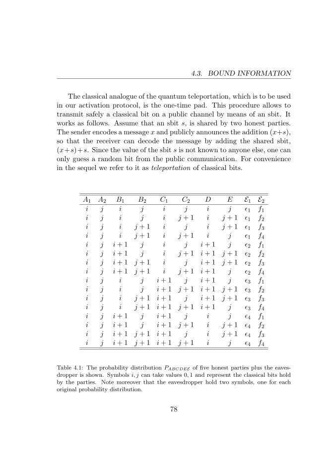
The connection between information-theoretic key agreement and quan-tum entanglement purification has led to several analogies between the twoscenarios. The most intriguing open question is the conjectured existenceof bound information, a classical analog of bound entanglement. It refers toclassical correlations that, despite containing some intrinsic secrecy, do notallow its extraction by means of any protocol based on local operations andpublic communication between two honest parties. Despite some evidenceof its existence in the bipartite scenario, a proof is still missing. By exploit-ing the analogies between the quantum and classical scenario, we providetwo probability distributions that are not key-distillable by two-way com-munication protocols and therefore may have bound information. Then,we show that the combination of these two distributions leads to a positivesecret-key rate. This result thus supports the idea that the secret-key rate,a fully classical information concept, may be a non-additive quantity.

Moving to the multipartite scenario, the freedom offered by consider dif-ferent bipartitions of the honest parties considerably simplifies the problemand allows showing that bound information indeed exists. We have shown

13

CONTENTS

that several properties of bound entanglement, such as superactivation orunlockability, can be translated to bound information. We also provide an-other common feature of both resources. Although non-distillable, they canhelp to distribute pure state entanglement and multipartite secret correla-tions, respectively, when a new party is added to the considered scenario.

We move later to deepen the connection between privacy and non-locality. With this aim, we consider the private states, that is, those quan-tum states from which two or more honest parties can extract a secret key.We show that all private states are non local, in the sense that they al-ways violate the CHSH inequality. The proof is completely general since itapplies for any dimension and any number of parties.

Finally, we study the relation between non-locality and randomness cer-tification. It is well known that non-local correlations must have randomoutcomes to be compatible with the no-signalling principle. Thus, within ano-signalling theory, the violation of a Bell’s inequality can be considereda certificate of randomness. Still, it is not known under which circum-stances one can certify maximal randomness. We show that the symmetryof a Bell’s inequality plus the uniqueness of the probability distributionmaximally violating it can be used to certify maximal randomness. Theadvantage of our method relies on the fact that simple analytical consider-ations can bring insightful results on randomness certification via quantumnon-locality without the need of any heavy numerical computation.

The dissertation ends up with an overview of the obtained results andpossible follow-up research directions.

14

Chapter 1

Introduction

This chapter presents the context and main results obtained during the PhDThesis. While the formal treatment will be given in the next chapters, wegive here the questions and the motivations that have led to the work thatwe report in this thesis. Finally, a graphical scheme is sketched representingthe connections analysed in this dissertation.

1.1 Introduction

Quantum Information Theory (QIT) can be understood as the effort to gen-eralise Classical Information Theory to the quantum world. The fact thatvery-small scale Physics differs considerably from that of macroscopic ob-jects implies a richer structure of the new theory. Although its formulationlacks the intuition common to the old theories of Nature, the accurate pre-dictions of quantum phenomena do of Quantum Mechanics a fundamentaltool of investigation.

Among others, phenomena as entanglement and the existence of non-local correlations make this theory very special, since these effects are notpossible for classical systems. Although intrinsically non-intuitive, thesestrange effects have been shown to lead to intriguing applications with noclassical analogue. In particular, the comparison of the same task based

15

1.2. MOTIVATIONS AND RESULTS

on classical and quantum technology has almost always seen a significantadvantage of the latter over the former. To cite only few, the possibilityof sharing a secret key [BB84, Eke91], to teleport the unknown state of aquantum particle [BBC+93] and to factorise huge numbers in a polynomialtime [Sho94] is something possible at a quantum level. But this is just asmall sample of the new range of possibilities offered by the introduction ofQuantum Physics in the Information world.

Despite the vast amount of successes achieved by QIT in these years,many interesting fundamental questions are left unanswered. Being a fieldunder current development, many powerful resources appear whose rela-tions are still not completely understood. At a more foundational level,and despite the great effort by the scientific community, simple questionsremain unanswered, leaving the feeling that very novel ideas are required.

1.2 Motivations and Results

Quantum Information Theory, like Classical Information Theory, is mostlya theory about resources: quantum effects are seen as resources for informa-tion processing. But the new theory is richer than its classical counterpartand new resources appear in the formalism, such as quantum bits, entangledqubits, private quantum bits, non-local correlations or intrinsic randomness.The main scope of this thesis is to establish qualitative and quantitativeconnections among these different quantum information resources. In whatfollows, we introduce the questions addressed in this work.

Q1. Is the secret key rate an additive quantity?Among the many weird effects that quantum systems present, the non-additivity concept plays an important role. In the quantum realm, the jointprocessing of two quantum resources is often better than the sum of the tworesources. Activation is the strongest manifestation of non-additivity. Sucha process can be understood as the capability of two objects to achieve agiven task that is impossible for each of them when considered individually.

16

CHAPTER 1. INTRODUCTION

Figure 1.1: Scheme of the thesis. The drawing above shows the connections analysed inthis dissertation. In chapters 3 and 4 the likely correspondence between entanglement andsecret-key agreement is discussed providing some evidence among bound entanglementand bound information (R1, R2). In chapters 5 a general proof is given that states whichprovide secret correlations are non-local (R3). Finally in chapter 6, the non-locality ofquantum distribution is used to certify the presence of genuine randomness (R4).

17


Many examples are known nowadays of activation of quantum resources:the entanglement of formation, the distillable entanglement and the classi-cal and private capacities of a quantum channel can be activated. From aclassical point of view, while additivity is known to hold for the capacity ofclassical channels, it is unknown whether there may be classical informa-tion resources that can be activated. Here we study whether the classicalsecret-key rate can be activated. That is, is it possible to combine classicalresources obtaining a positive secret-key rate, despite no secrecy can beextracted from them individually?

R1We provide two probability distributions conjectured to have bound in-formation, hence from which it is conjectured that no secret key can beextracted (even by two-way communication protocols), when taken individ-ually, but that lead to a positive secret-key rate when combined. In order toprove this result we exploit the close connection between the information-theoretic key agreement and the quantum entanglement scenario.

Q2. Can bound information be super-activated and unlocked?Entanglement is one of the key resources that distinguishes Quantum Infor-mation Theory from its classical counterpart. The impossibility for remoteparties to create an entangled state between particles that never inter-acted in the past, makes this feature really unique for communication pur-poses. The presence of pure entanglement constitutes the main ingredientfor devising protocols that allow distant users to share secrecy. In the key-agreement scenario, several parties, including a possible adversary, sharepartially correlated classical information. The goal of the honest parties isto share secret correlations from the given initial ones, in such a way thatno information is known to the malicious party. The two scenarios sharethereby many interesting similarities. Despite the natural expectation thatall noisy entangled states can be brought to a pure form, the existence ofnon-distillable (bound) entangled states was shown. From the analogy be-tween the entanglement and key-agreement scenario, Gisin and Wolf gave

18


evidence for the existence of a classical analog of bound entanglement, theso-called bound information. Bound information refers to classical corre-lations that do contain some intrinsic secrecy but that cannot be distilledinto a pure secret key by means of any protocol. It is known that boundentanglement can be super-activated and unlocked. Given the existing con-nections between the two scenarios, do the same properties also hold forbound information?

R2We present the analogs of finite copy super activation and unlockabilityof bound entanglement for classical secret correlations. In order to do so,we provide examples of multipartite classical probability distributions withbound information and prove that they can be super-activated and un-locked. Additionally, we provide a new property that is shared by boundentanglement and information. Bound entanglement (information) can beused for distributing pure state entanglement (secret correlations) by Lo-cal Operation and Classical Communication (LOCC) (Local Operation andPublic Communication, LOPC). More precisely, in the quantum scenario,we show that the a tripartite entangled pure state can be extended byLOCC to a four partite entangled state with the help of a bound entan-gled state shared among all the parties. The classical analog follows: whenbound information is shared by four parties a secret bit of three parties canbe distributed among the four using LOPC protocols.

Q3. What is the relation between privacy and non-locality?A common future to every successful theory concerns the possibility of inter-conversion between apparently different kind of resources. Two key topics inQuantum Information Science are Quantum Key Distribution (QKD) andNon-Locality. Both rely on the existence of shared entanglement betweentwo or more separated parties. Private states are those entangled statesfrom which a perfectly secure cryptographic key can be extracted. An ex-ample of such a state is a maximally entangled state, but there are otherprivate states that are not maximally entangled. Actually, while a maxi-

19


mally entangled state violates a Bell’s inequality, this is not known a priorifor the whole set of private states. Understanding their non local propertieswould thus bring to a better comprehension of the relation between secret-key extraction and violation of Bell’s inequalities in the quantum regime.Thus, are all private states non-local? If so, what kind of non-locality dothey show?

R3We show that all states belonging to the class of private states violate theCHSH-Bell inequality. This result is general, as our proof works for any di-mension and any number of parties. Private states, then, not only representthe unit of quantum privacy, but also allow two distant parties to establisha different quantum resource, namely non-local correlations. These statescontain the strongest form of entanglement as they can give raise to cor-relations with no classical analogue. More in general, our findings pointout an intriguing connection between two of the most intrinsic quantumproperties: privacy and non-locality.

Q4. How can we certify genuine randomness?Non-locality and genuine intrinsic randomness have been the subject of ac-tive interest since the early days of quantum physics. Initially, this interestwas mainly derived from their foundational and fundamental implicationsbut recently it also has acquired a practical aspect. Recent developments indevice independent applications have heightened the need to quantify boththe randomness and non-locality inherent in quantum systems. A key pointis the guarantee that randomness does not originate from a mere lack ofknowledge of the observed system. This allows one to certify that the quan-tified randomness holds for all observers irrespective of their knowledge ofthe system. To do it more concrete, classical systems can exhibit at mostpseudo randomness since they can always, in principle, be simulated by amixture of deterministic systems. This result is no longer valid for systemswhose correlations violate a Bell inequality. Non-locality is a necessarycondition, then, for certifying the presence of true intrinsic randomness.However, which Bell tests are necessary to certify maximal randomness?

20


R4We provide a simple recipe to detect Bell tests that allow the certificationof maximal randomness. These arguments exploit the symmetries of Bellinequalities and assume the uniqueness of the quantum probability distribu-tion maximally violating it. We show how these arguments can be appliedto intuit the randomness intrinsic in a probability distribution without re-sorting to numerical calculations. In particular, we use these argumentsto provide Bell tests based on two-outcome measurements that allow thecertification of two random bits, the highest randomness attainable in thisscenario.

1.2.1 Outline of the Thesis

The thesis in exam is organized as follows. Chapter 2 introduces the ba-sic concepts to understand the results presented in the following chapters.Quantum entanglement, secret correlations, non-local correlations and ran-domness are briefly explained focusing especially on those features thatare relevant to our findings. In chapter 3 we provide an evidence for theactivation of the secret-key rate in the bipartite scenario. In chapter 4the one-to-one correspondence between bound entanglement and bound in-formation is presented. We show that superactivation, unlockability andpurification assistance of the Smolin state do have a classical analog. Inchapter 5 we show the general proof of the non-locality of private states.In chapter 6 we move to the certification of maximal quantum randomnessin Bell tests. Chapter 7 concludes the thesis reviewing briefly our findingsand presenting future perspective. Lastly, several appendices are providedto explain technical issues in more detail.

21


22

Chapter 2

Background

The aim of this section is to present four strictly related concepts thatwill be used in the next chapters, namely, quantum entanglement, secretcorrelations, non-local correlations and random bits. As already stated, themain goal of this thesis is to establish connections among them helping tobetter understand their role for information purposes.

In this chapter after a brief historical review, we give the necessarybackground for discussing the technical results shown in this dissertation.We will present the definitions, notations and techniques that will be usedin later chapters, as well as several clarifying examples.

2.1 Historical remarks

The first decades of the twentieth century saw an emerging contrast be-tween the experimental results shown by the atomic world and the predic-tions inferred from the existing framework of classical theory of Science.What many brilliant physicists understood very soon was that a changeof paradigm was needed to explain those astonishing facts. What perhapsthey did not know was that the required change was so radical.

A counter intuitive concept as that of wave-particle duality was shownto be an intrinsic feature of matter and radiation. As a consequence the su-

23

2.1. HISTORICAL REMARKS

perposition principle was straightforwardly extended to what was definedas the wave function (or state) of a quantum system. But this was notall. A distinct feature was still missing: in 1927 W. Heisenberg provided anheuristic argument showing a fundamental limit on the precision with whichcertain pairs of physical properties of a particle (such as position and mo-mentum) could be simultaneously known. The uncertainty relations markedanother fundamental difference between classical and quantum mechanics:the one-to-one correspondence between the physical properties of the con-sidered object (and thus the entities of the physical world) and their formaland mathematical representation in the theory came to a sudden end.

The main pillar of the novel view, known as Copenaghen interpretation,was constituted by the fact that a quantum system could not be thought ofas possessing individual properties independently of the experimental ar-rangements. In a nutshell, Bohr and coworkers were destroying the intuitiveand consolidate concept of reality, deeply rooted in the minds of scientistsand layman alike. This was enough to stimulate an immediate reply to theunacceptable conception that the new Physics seemed to require.

In 1935, A. Einstein, B. Podolsky and N. Rosen (EPR) published aseminal paper [EPR35] whose main claim was to show the incompletenessof the quantum theory. In the same year, Schrodinger coined the term ”ver-schranckter Zustand” (entangled state), to refer to the highly singular stateused by EPR. He immediately emphasized its non-classical implications:

When two systems, of which we know the states by their respec-tive representatives, enters into a temporary physical interactiondue to known forces between them, and when after a time of mu-tual influence the system separate again, then they can no longerbe described in the same way as before, viz. by endowing eachof them with a representative of its own. I would not call thatone but rather the characteristic trait of quantum mechanics,the one that enforces its entire departure from classical lines ofthought.

On the other hand the answer of Bohr to EPR did not take much to arrive.It was the beginning of a long and enlightening debate between two of the

24

CHAPTER 2. BACKGROUND

greatest scientists of the 20th century.In the meanwhile, in Computer Science, another revolution was tak-

ing place. In the the ’40s, Claude Shannon published seminal remarkablepapers laying the foundations for the modern theory of information andcommunication. The key step taken by Shannon was to mathematicallydefine the concept of information. Two main questions were predominant:first, what kind of resources is required to send information over a commu-nication channel? Second, could information be transmitted reliably whensent over a noisy channel?

The answer to the first question was provided in his noiseless channelcoding theorem, which quantifies the amount of physical resource neededto store the output from an information source. The second answer, thenoisy channel coding theorem, instead, identifies the maximal noise that anerror correcting code can afford in order to protect and then conserve theoriginal sent information. Many devices we use daily strongly rely on theachievements of the classical theory of information.

If the long debate between Bohr and Einstein brought many insight-ful results, the key question of EPR remained unanswered. The break-through came only in 1964, when John Bell, formulating the EPR dilemmain form of assumptions, showed that measurements on an entangled stateled manifestly to a contradiction of the assumptions. With Werner’s words[WW01b], the Bell’s theorem was so crucial that:

It is hardly possible to underrate the importance of this discov-ery, which made it possible to rule out not just a particularscientific theory, but the very way scientific theories had beenformulated for centuries.

Despite its importance, it took almost thirty years for the scientific com-munity to really exploit the importance of Bell’s theorem: a practical ap-plication was needed to attract a widespread attention.

Almost in the same period moved by a better understanding of howphysics constrains our ability to use and manipulate information, Landau-rer came to the conclusion that Information is physical [Lan61, Lan92].

25

2.1. HISTORICAL REMARKS

The main argument discussed, was that information is not a disembodiedabstract entity, but it is always tied to a physical representation. In otherwords, the mathematical terms in which a given theory is expressed aresubject to the limitations (and benefits) of our physical world.

Quantum mechanics had a chance.Unlike classical physics, the act of acquiring information about a quan-

tum system inevitably disturbs the state of the system. The first conse-quence (the cons) of this fact is that a reliable cloning of quantum infor-mation is impossible [WZ82]. The second (the pro) is that the security of akey-distribution protocol could be guaranteed by it. An eavesdropper couldbe intercepted by the honest parties due to his/her inevitable introductionof errors in the channel [BB84]. Another remarkable consequence of no-cloning was represented by the impossibility of sending information fasterthan the speed of light (signalling) between remote parties.

Einstein’s relativity was safe.

Since the ’80s many of the central results of classical information theorywere shown to have more powerful quantum analogs [CT91, NC00]. Quan-tum Information Theory has since then emerged as a vigorous research fieldcombining concepts and tools from Physics, Computer Science, Mathemat-ics and Engineering. New quantum algorithms [Sho94] have been foundproviding an efficient solution to problems (integer factorization and dis-crete logarithm) for which there is no known efficient classical algorithm.These algorithms take classical inputs (such as the number to be factored)and yield classical outputs (the factors), but obtain their speedup by usingquantum interference among computation paths during the intermediatesteps . In quantum communication, entanglement has been shown funda-mental for the teleportation of quantum states [BBC+93] and for super-dense coding [BW92]. Moreover, entanglement is a key ingredient for theachievement of security in cryptographic scenarios and necessary for theviolation of Bell’s inequalities.

In fact, the connection between cryptography and non-locality was verysmartly addressed by Ekert in 1991 [Eke91]. He showed that the securityof the protocol could be guaranteed by the violation of a Bell’s inequality.

26


This result was the missing application which made clear the importance ofthe Bell’s theorem and from which many interesting ideas and applicationsborn under the label Device Independent.

Device-Independent Quantum Information Processing can be consid-ered nowadays as a new paradigm for quantum information processing.The goal is to design protocols for solving relevant information tasks with-out relying on any assumption on the devices used in the protocol. Forinstance, device-independent key distribution can certify shared secrecy be-tween two honest users independently of the devices that have been used inthe distribution (DIQKD). Another successful application allowed by thisapproach is the generation of genuine randomness (DIRNG). While it iswell known that no real randomness can be generated through determinis-tic procedures, the correlations exhibited performing certain measurementson entangled states, necessarily certify the randomness of the obtained out-comes. The certificate in this case is again provided by the violation of aBell’s inequality.

2.2 Quantum Entanglement

The deep way that quantum information differs from classical informationinvolve the properties, implications and uses of quantum entanglement. Thevast majority of quantum information applications are mainly based on thecreation and manipulation of entangled states shared by remote parties.This section presents the main features of entangled states, including thebasic tools and problems behind their definition.

2.2.1 Bipartite Scenario

A composite pure system |Ψ〉AB, belonging to two distant parties A and B(also called Alice and Bob in the sequel) is said to be entangled wheneverit cannot be written in a factorized (or product) form, that is

|Ψ〉AB 6= |ψ〉A ⊗ |ψ〉B, (2.1)

27

2.2. QUANTUM ENTANGLEMENT

where |ψ〉A and |ψ〉B represent states in A and B locations.Being the pure state description limited by the presence in Nature of

decoherence processes, the density matrix formalism is used to fully charac-terize any quantum (mixed) state. In contrast to a pure state |Ψ〉AB, whichis represented as a vector in a Hilbert space H = HA ⊗HB, a mixed stateis described by a density matrix, i.e. a hermitian, positive-definite linearoperator of trace one, acting on the same Hilbert space. In this case aquantum state is said entangled whenever it cannot be written as a convexcombination of projectors on product states [Wer89]:

ρAB =k∑i=1

pi|ψi〉〈ψi|A ⊗ |ψi〉〈ψi|B. (2.2)

Beyond this mathematical definition, an entangled state has a clear oper-ational meaning. While two distant observers can prepare a global state(2.2) by performing Local Operations (LO) on their subsystems and ex-changing Classical Comunications (CC) among them, an entangled staterequires a joint preparation. In other words, LOCC protocols cannot create(or increase) entanglement.

A maximally entangled state (or Bell pair) of two qubits represents themost representative example of a bipartite entangled state and is an essen-tial ingredient in many applications of quantum information theory [Ben95].Various equivalences are known: one shared Bell pair plus two bits of clas-sical communication can be used to teleport one qubit [BBC+93] and, con-versely, one shared Bell pair plus a qubit can be used to send two bitsof classical communication via superdense coding [BW92]. It is formallydefined (in the computational basis {|0〉, |1〉}) as:

|φ+〉 =1√2

(|00〉+ |11〉)AB (2.3)

and its relevance for communication purposes is due essentially to two mainfacts: first, for each projective measurement by one of the observers, thereexists another measurement by the other observer giving perfectly corre-lated results. Second, being a pure state, no third party can be corre-lated with it. State (2.3) represents the basic unit of entanglement and is

28


also known as ebit, for entangled bit. This is because an asymptoticallylarge number of copies of an arbitrary pure entangled state can be con-verted into another asymptotically large number of ebits in a reversibleway [BBPS96, LP99]. For example, suppose that Alice and Bob have alarge number N of pairs of particles, each pair in some pure non-maximallyentangled state, |ψ〉 =

√p|00〉+

√1− p|11〉, where 0 < p < 1/2. By acting

locally and communicating on a classical channel, they can end up with asmaller number of pairs each in the maximally entangled state (2.3). Thisnumber correspond to NE(ψ), where E(ψ) is the entropy of entanglementof state ψ:

E(ψ) = −trρA log ρA = −trρB log ρB (2.4)

where ρA, ρB are the reduced density matrix of the state ψ for A and Brespectively:

ρA (ρB) =(p 00 1− p

)This process is known in literature as concentration of entanglement. Theinverse process, of transforming NE(ψ) ebits in N pairs of ψ is also possibleand known as dilution. Remarkably, the entropy of entanglement providean exact quantification of the pure state entanglement, and moreover asclear from the previous example, this quantity is conserved in the processesof concentration and dilution. In the mixed state scenario other measures ofentanglement have been proposed. To better clarify this point, the followingsection lists some well known quantifiers and problems of the theory ofentanglement.

2.2.2 Quantifying and Distilling Entanglement

As soon as one consider the more realistic scenario of converting pairs ofmixed states into pure maximally entangled states, the answer becomesharder.

A generalization of the dilution process can be stated as follows. Let usconsider the case in which two (or more) separated parties aim at preparingm copies of a state ρ by LOCC. The answer to the question of how many

29

2.2. QUANTUM ENTANGLEMENT

ebits they need in order to obtain m copies of the state ρ is provided by theentanglement cost. In particular, the entanglement cost [HHT01], denotedby Ec, quantifies the number of ebits per copy asymptotically needed forthe formation of the given quantum state by LOCC. For pure states Eccoincides with the entropy of entanglement previously defined.

The inverse problem is known as distillability problem and is a gen-eralization of the concentration process. A composite mixed state ρABisdistillable whenever Alice and Bob can transform k copies of it into a statearbitrarily close to the maximally entangled state (2.3) by LOCC. Thereby,the entanglement of distillation [BDSW96], denoted by ED, quantifies theamount of ebits per copy (of the given state) that can be obtained from itby LOCC.

For a state ρAB, Ec(ρAB) > 0 implies that the state is entangled, whileED(ρAB) > 0 indicates that some pure entanglement can be extracted fromit. Clearly, it holds that Ec ≥ ED, as one cannot extract from a state moreentanglement than needed for its preparation. Note that in the pure statecase, Ec = E = ED, due to the reversibility of the concentration anddilution processes.

Interestingly, there are states that display an intriguing form of irre-versibility: despite having a positive entanglement cost (Ec > 0), they arenon-distillable (ED = 0). These states are called bound entangled [HHH98].Consequently, the whole set of entangled states is composed of distillable,or free entangled states, and bound entangled states.

As said, detecting whether a given state is non-distillable is in principle avery hard question, as one has to prove that no LOCC protocol acting on anarbitrary number of copies of the state is able to extract any pure entangle-ment. However, a very useful result derived in [HHH98] shows that a quan-tum state that remains Positive under Partial Transposition [Per96] (PPT)is non-distillable. Whether Non-Positivity of the Partial Transposition, orNegative Partial Transposition (NPT), is sufficient for entanglement distill-ability is probably the main open question at the moment in EntanglementTheory. Evidence [DCLB00, DSS+00] has been given for the existence ofNPT states that are bound entangled (see however [Wat04]). Note that theexistence of these states would imply that the set of non-distillable states

30


is not convex and that entanglement of distillation is non-additive [SST01].A necessary and sufficient condition for the distillability of a quantum stateis provided by the following

Theorem 1. A state ρ acting on H = HA ⊗HB is distillable if and onlyif there exist a finite integer number n ≥ 1 and two dimensional projectorsP : H⊗nA → C2 and Q : H⊗nB → C2 such that the state

ρ′ = (P ⊗Q)ρ⊗n(P ⊗Q)† (2.5)

is entangled.

Actually, since the resulting state acts on C2 ⊗ C2, this is equivalent todemand that ρ′ is NPT, as this condition is necessary and sufficient forentanglement in the two-qubit case [HHH96]. Furthermore, it is worthmentioning here that, if such a projector exists for some number k of copies,the state is said to be k − distillable.

2.2.3 Multipartite Scenario

Characterizing the entanglement in a multipartite scenario, in which moreparties are provided with some arbitrary quantum state ρ, is quite morecomplex than in the previous case. This difficulty is connected with thefact that, in the multipartite scenario, one can have many partitions of theremote parties, so the quantum state can be entangled with respect to someof them, while separable in the remaining ones. As before, a straightforwarddefinition of full separability is easily generalized. A quantum state ρ of Nparticles which can be factorized into local states:

ρ =∑i=1

piρi1 ⊗ ρi2 . . .⊗ ρiN (2.6)

is called completely separable. As announced, for a complete characteriza-tion of multipartite entanglement is necessary to consider all possible group-ings of particles of the total system and study the entanglement among suchgroups. Consider an N -partite quantum state ρ and a possible partition

31

2.3. SECRET CORRELATIONS

P={p1, p2, . . . , pk} of the same, where k ≤ N . The state ρ is said k-separablein the P partition if it can be written as:

ρ =∑i=1

piρ1i ⊗ ρ2

i . . .⊗ ρki (2.7)

where ρj i represent the quantum state of the jth group of particles in theP partition. If the N -partite quantum state does not admit any sort ofdecomposition (2.7), this means that all particles are entangled with eachother, so the state is said genuine multipartite entangled.

Another difficulty in the multipartite scenario comes from the fact thatit is not known whether it is possible to define a unit of multipartite entan-glement [LPSW05]. The question of which is the minimal set of states thatN parties should share in order to generate any N -partite pure state byusing LOCC in the asymptotic scenario in a reversible manner is still open.This set it has been termed MREGS from minimal reversible entanglementgenerating set. In the (asymptotic) tripartite scenario, for example, the set

G3 = {|GHZ〉ABC , |EPR〉AB, |EPR〉AC , |EPR〉BC}

where |EPR〉ij is the ebit (2.3) between party i and j and |GHZ〉 is thestate:

|GHZ〉 =1√2

(|000〉+ |111〉) (2.8)

shared by ABC in the computational basis, was conjectured to be a goodcandidate for generating all tripartite pure states. Unfortunately, in Ref.[AVC03] a counterexample was provided falsifying this conjecture. Actually,it is even known whether an MREGS consisting of a finite number of statesexists.

2.3 Secret Correlations

The main scope of this section is to introduce the secret-key agreement sce-nario together with the natural concept of secret correlations. This scenario

32


consists of two honest parties, again Alice and Bob, who have access to cor-related information, described by two random variables X and Y . Thesevariables are also correlated to a third random variable Z that belongs toan adversarial party, the eavesdropper Eve, denoted by E. All the correla-tions among the three parties are described by the probability distributionP (XY Z). The aim of the honest parties is to map their initial correlationsinto a secret key by Local Operations and Public Communications(LOPC),which is the natural set of operations at their disposal.

They will share a perfect secret bit whenever P (XY Z) is such that theeavesdropper is factored out, P (XY )× P (Z), and their variables (X,Y =0, 1), are perfectly correlated and random, P (X = Y = 0) = P (X = Y =1) = 1/2. This scenario is defined as the classical analogue of the entangle-ment scenario. Here, a secret bit represents the equivalent of a maximallyentangled state. This analogy is mainly based on the fact that secret cor-relations cannot be created by LOPC protocols, in the same fashion asentanglement cannot be created by LOCC protocols.

Additionally, other reasonable analogies have been shown in [CP02]. Asin the quantum scenario, if the parties share N copies of a classical resourcedistributed according to:

P (X = i, Y = j, Z = k) = δijpiP (Z = k) (2.9)

they can transform it reversibly in a new distribution Q(X = i, Y = j, Z =k) = δijqiQ(Z = k). This is the classical equivalent of the concentrationor dilution process. This follows from the fact that (2.9) can be obtainedby measuring a pure quantum bipartite in its Schmidt basis. Since theentanglement concentration process is performed in the Schmidt bases, thequantum protocol directly translates into a classical protocol for distribu-tions (2.9). As for the quantum case, the entropy of secrecy, quantifies theamount of sbit, qi = 1/2, that can be produced per copy of the originaldistribution pi as follows:

K

N= −

∑i

pi log2 pi

33


The picture becomes harder when considering correlations P (X = i, Y =j, Z = k) in which the eavesdropper is not factored out. This case isanalogous to the mixedness of a pure state under the decoherence effects ofthe environment (see eq. (2.1)). Similarly as above, the goal in this case isto quantify its secrecy content.

The classical analogue of Ec is the information of formation, denotedby If [RW03]. It is said that the probability distribution P (XY Z) containssecret correlations (or secret bits) whenever If (P (XY Z)) > 0. For distil-lation, the natural classical analog is the secret-key rate [MW99], denotedby S(X : Y ‖Z), which quantifies the number of secret bits that can bedistilled from given correlations by LOPC. Thus, given the three randomvariables (X,Y, Z), if Bob’s random variable Y provides more informationabout Alice’s X than Eve’s Z does (or vice versa), then this advantage canbe exploited for generating a secret key. This can be expressed as:

S(X : Y ||Z) ≥ max{I(X : Y )− I(X : Z), I(Y : X)− I(Y : Z)} (2.10)

where I(P : Q) is the mutual information among two random variables Pand Q:

I(P : Q) = H(P ) +H(Q)−H(PQ) (2.11)

and H(S) is the Shannon Entropy of the random variable S. Althoughin Ref. [CK78], the positivity of the relation (2.10) was shown to be asufficient condition for one-way communication secret-key agreement, newprotocols were later devised able to give a positive secret key rate even forthose cases in which the left hand side of (2.10) is negative.

In [Mau93], Maurer introduced the advantage distillation (AD) proto-col, which allows two honest parties to extract a secret key even in casesin which Bob has less information than Eve about Alice’s symbols. Crucialto achieve this task is feedback, that is, two way communication betweenthe honest parties. The general structure of an AD protocol is as follows[AGS03] (without loss of generality we assume that Alice’s and Bob’s vari-ables have the same size d): Alice first generates randomly a value ζ. Shechooses a vector of N symbols from her string of data, a = (a1, . . . , aN ),and publicly announces their positions to Bob. Later she sends him the

34


N -dimensional vector a whose components ak are such that ak ⊕ ak = ζholds ∀k. Here, ⊕ is the sum modulo d. Bob sums a to his correspond-ing symbols. If he obtains always the same value χ, then he accepts (thismeans that with very high probability χ = ζ) otherwise both discard theN symbols.

Although its yield is very low with increasing N , AD protocols allow thehonest parties to distill a key even in a priori disadvantageous situationsin which Eve has more information than Bob on Alice’s symbols. Suchprotocols are used in what follows to estimate the distillability propertiesof the given correlations. Obviously, the fact that one is unable to mapsome correlations into a secret key by AD protocols does not mean thatthese correlations are non-distillable. At best, it can be interpreted assome evidence of non-distillability.

The protocols introduced so far give us a lover bound on the secret-keyrate in the one and two-way communication scenario, respectively. We nowmove to describe known upper bounds on the secret-key rate. Intuitively,the fact that no secret key can be derived by the honest parties wheneverBob’s information is independent from Alice’s random variable, given Eve’sinformation is captured by the inequality:

S(X : Y ||Z) ≤ I(X : Y |Z).

If Alice’s and Bob’s symbols are uncorrelated I(X : Y |Z) = 0, henceS(X : Y ||Z) = 0. However, it was realized that this bound is not tight.The possibility for an adversary to process her variable Z, i.e., to send Zover some channel characterized by P(Z|Z), can lead to situations in whichI(X : Y |Z) < I(X : Y |Z). To take this in account, the intrinsic informa-tion [MW99] must be used. It is defined as the minimal mutual informa-tion between X and Y conditioned on Z, where Z is the best (from theeavesdropper’s point of view) mapping of the random variable Z that theeavesdropper can perform, i.e. Z → Z:

I(X;Y ↓ Z) := minPZ|Z

[I(X;Y |Z) : PXY Z =

∑z

PXY Z · PZ|Z

](2.12)

35


In Ref [CRW03] it was shown that there is no loss of generality in consider-ing the output alphabet Z of the same size of the input alphabet Z. Thismeasure plays a relevant role in key-agreement scenarios since it allows tobound the two main quantifiers previously defined:

S(X;Y ‖Z) ≤ I(X;Y ↓ Z) ≤ If (X;Y |Z) (2.13)

Along the connection with entanglement theory, a main open questionwas risen in Ref. [GW00]: is it possible to characterize classical correlationswhich cannot be distilled but which are shown to contain strictly positiveinformation of formation, or simply I(X;Y ↓ Z) > 0? A distributionP (XY Z) is said to contain bound information if the following relationshold:

S(X : Y ||Z) = 0 I(X;Y ↓ Z) > 0. (2.14)

In a nutshell, although these correlations cannot be distributed by LOPCthey would not allow the honest parties to distill secrecy by LOPC, evenwhen sharing an infinite number of instances of P (XY Z).

If shown, these correlations would constitute a classical cryptographicanalog of bound entanglement [GW00]. Compared to the entanglementscenario, identifying a single example of non-distillable correlations is muchharder, due to the lack of a simple mathematical criterion, as the PartialTransposition [Per96], to detect it. In a multipartite scenario, say of threehonest parties plus an eavesdropper, the possibility of splitting the honestparties into different bipartitions hugely simplifies the problem and, indeed,there are examples of correlations that require secret bits for the preparationand from which no secret bits can be extracted [ACM04]. The problemremains open for two honest parties, although evidence has been providedfor the existence of bound information [GW00].

Finally, another concept that we will use in the sequel is that of bina-ryzation, which can be understood as the classical analog of the quantumprojection onto 2-qubit subspaces used in Theorem 1. As in the quantumcase, Alice and Bob agree on two possible values, not necessarily the same,

36


and discard all instances in which their random variables take different val-ues. Then, they project their initial distribution onto a smaller (and usuallysimpler) two-bit distribution.

2.3.1 Link between entanglement and secret key-agreement

It is clear from the previous discussion that the entanglement and secret-key agreement scenarios have a similar formulation. One can go furtherand establish connections between the entanglement of bipartite quantumstates and the tripartite probability distributions that can be derived fromthem [GW00]. Not surprisingly, the transition from quantum states toclassical probabilities is through measurements (on the quantum states).Note also that, while in the quantum case the state between Alice andBob also specifies the correlations with the environment, possibly undercontrol of the eavesdropper, in the classical cryptographic scenario it isessential to define the correlations with the eavesdropper for the problemto be meaningful.

As mentioned, if Alice and Bob share a state ρAB, the natural way ofincluding Eve is to assume that she owns a purification of it. In this waythe global state of the three parties is a pure tripartite |ψABE〉 such thatρAB = trE (|ψABE〉〈ψABE |). After this purification, measurements by thethree parties, MX , MY and MZ , respectively, map the state into a tripartiteprobability distribution:

P (X,Y, Z) = tr (MX ⊗MY ⊗MZ |ψABE〉〈ψABE |) (2.15)

It has been shown that: i) if the initial quantum state is separable, thereexists a measurement by the eavesdropper such that the probability distri-bution (2.15) has zero intrinsic information for all measurements by Aliceand Bob [GW00, CLL04] and also zero information of formation [AG05]and ii) if the initial state is entangled, there exist measurements by Aliceand Bob such that the probability distributions (2.15) has strictly positiveintrinsic information for all measurements by Eve [AG05].

37

2.4. NON-LOCAL CORRELATIONS

2.4 Non-Local Correlations

While the question of EPR [EPR35] led immediately Shrodinger [Sch35] torecognize the intrinsic novelty of the entanglement, it took almost thirtyyears to rule out, at least theoretically, the basic hypothesis of a theory ala EPR.

In 1964 J. S. Bell [Bel64] provided a mathematical argument demon-strating that the probabilities of the outcomes obtained when applyingsuitable measurements on some entangled states could not be explained bya local realistic model as the one suggested by EPR.

2.4.1 Bipartite scenario

To illustrate the elegant theorem provided by Bell, it is sufficient to con-sider two distant observers (A and B) able to perform m possible localmeasurements (x, y = 1 . . .m) of r possible results, (a, b = 1 . . . r), on thepart of a shared physical system ρ which they can access to. As in a blackbox approach, it is enough to say that for each run of the experiment, Aliceand Bob can freely choose between a finite number m of settings x and y,obtaining always one outcome each, a and b, among d possible results.

After a sufficient large number of runs, they can thus estimate theirconditional probability distribution P (ab|xy)ρ. Moreover, two additionalrequirements are needed: (i) each local measurement defines space-like sep-arated events, and (ii) the choice of the measurement setting at each sideis made at the moment of measuring. The observed correlations P (ab|xy)ρare compatible with a local realistic theory [Bel64] when they can be de-rived by averaging over some hidden (classical) variable λ the product ofthe two local distributions PA(a|x, λ), PB(b|y, λ):

PL(ab|xy)ρ =∫PA(a|x, λ)PB(b|y, λ)σ(λ)dλ, (2.16)

where σ(λ) refers to the probability measure according to which λ is dis-tributed. The locality condition imposes that the local distributions PA(a|x, λ),PB(b|y, λ) can only depend on the chosen setting and on the hidden-variable λ, on which no restrictions are generally imposed. Model (2.16) was

38


shown to be equivalent to the existence of a joint probability distributionP (a(1), . . . , a(m), b(1), . . . , b(m)) involving all local measurements (from 1 tom), such that the marginal probabilities reproduce the observed measuredoutcomes of the given experiment [Fin82].

The distribution P (ab|xy)ρ (obtained by measurements on some physi-cal system ρ) is said non-local, if it does not admit a local description (2.16).If ρ is a quantum state shared by two distant observers, the distributionP (ab|xy)ρ reads:

PQ(ab|xy)ρ = tr(ρMa|x ⊗Mb|y), (2.17)

where the positive operators Ma|x and Mb|y satisfy the completeness rela-tion,

∑kMk|x = I, for k = a, b.

Bell showed that the correlations arising when certain measurements aremade on a composite system of two spins-1/2 particles in a singlet state1:

|ψ−〉 =1√2

(|01〉 − |10〉)AB (2.18)

with |0〉 and |1〉 representing the state up and down of the spin of a par-ticle, could not be expressed as (2.16). This was the evidence, at leasttheoretically, that quantum mechanics cannot be a local realistic theory.

But another step was still missing. Bell’s theorem in his original formu-lation was not directly testable in a lab, so in 1969, Clauser, Horne, Shimonyand Holt addressed this problem, deriving an inequality, nowadays knownas the CHSH [CHSH69] inequality, that could confirm experimentally thetheoretical result of Bell. Consider an experiment where two separated par-ties measure one of two possible observables, {A1, A2} and {B1, B2} withoutcomes ±1. For any local theory (2.16), the following inequality:

|〈A1B1〉+ 〈A1B2〉+ 〈A2B1〉 − 〈A2B2〉| ≤ 2 (2.19)

is bounded by 2. A violation of the CHSH inequality thus is sufficient forcertifying the presence of nonlocal correlations.

1Note that this state is unitarily equivalent to the state (2.3). Together with the twostates |ψ+〉 = 1√

2(|01〉+ |10〉) and |φ−〉 = 1√

2(|00〉 − |11〉) they form an orthonormal

basis on C2 ⊗ C2 known as Bell basis (or Bell states).

39

2.4. NON-LOCAL CORRELATIONS

The state (2.18), with opportune measurements can violate the CHSHinequality, up to 2

√2, showing then the non local character of quantum

mechanics. In particular, in the ’80s, it was shown by Tsirelson [Tsi80] thatthis is the maximal bound achievable by quantum mechanics. It is somhowsurprising that considering states on Hilbert spaces of higher dimensiondoes not lead to any improvement on this bound.

2.4.2 Multipartite scenario

The extension of a local model as (2.16) to the multipartite case, is ratherstraightforward:

PL(a1 . . . aN |x1 . . . xN ) =∫PA1(a1|x1, λ) . . . PAN (aN |xN , λ)σ(λ)dλ

(2.20)But, as already observed for multipartite entanglement, the presence ofmore parties implies a richer structure for the arising correlations. As aconsequence of that, it is not enough to talk only of local or non-localcorrelations, but the class of partially (non-)local correlations has to betaken in account. Partially local correlations are those that can be obtainedfrom an N -partite system in which subsets of the N parties form extendedsystems, which however behave local with respect to each other. Assumingthat parties 1, . . . , k form such a subset and the remaining parties k +1, . . . , N form the other, the partially local correlations can be written as:

PpL(a1 . . . aN |x1 . . . xN ) =∫P (a1 . . . ak|x1 . . . xk, λ)P (ak+1 . . . aN |xk+1 . . . xN , λ)σ(λ)dλ (2.21)

A model is said to have partially local correlations when the correlationsare of the form (2.21) or when they can be written as a convex combinationof the r.h.s. of (2.21) for different possible partitions of the N parties intotwo subsets. To make this more clear, we report in the following the earlymodel considered by Svetlichny [Sve87]. For N = 3, only three different

40


partitions are possible. Model (2.21) is thus extended to the form:

PpL(a1a2a3|x1x2x3) =∫dλ(P (a1|x1, λ)P (a2, a3|x2, x3, λ)p1σ1(λ)

+ P (a2|x2, λ)P (a1, a3|x1, x3, λ)p2σ2(λ)+ P (a3|x3, λ)P (a1, a2|x1, x2, λ)p3σ3(λ)) (2.22)

where P (a1, a2|x1, x2, λ) and the other two joint probability terms can beany probability distributions 2. Models whose correlations cannot be writ-ten in this form are said to contain genuine tripartite non-locality. Thegeneralization to more than three parties is straightforward.

2.4.3 Link between entanglement and non-locality

Given a separable state (2.6) it is always possible to construct a model whichreproduces correlations compatible with eq. (2.20). Let us show this forthe bipartite case. The N -partite generalization follows straighforwardlyfrom the bipartite proof. Consider the separable state (see eq. (2.2)):

ρAB =k∑i=1

piρiA ⊗ ρiB, (2.23)

on which two parties, A and B, can perform local measurements Ma|x,Mb|y. As already said the conditional probability distribution that A getsoutcome a when measuring x and B gets outcome b when measuring yreads:

pQ(ab|xy)ρ = tr(ρABMa|x ⊗Mb|y). (2.24)

2Recently it has been shown that even though these terms can be signalling, they needto respect a time order sequence [GWAN11].

41

2.5. RANDOMNESS

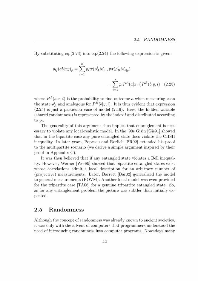
By substituting eq.(2.23) into eq.(2.24) the following expression is given:

pQ(ab|xy)ρ =k∑i=1

pitr(ρiAMa|x)tr(ρiBMb|y)

=k∑i=1

piPA(a|x, i)PB(b|y, i) (2.25)

where PA(a|x, i) is the probability to find outcome a when measuring x onthe state ρiA and analogous for PB(b|y, i). It is thus evident that expression(2.25) is just a particular case of model (2.16). Here, the hidden variable(shared randomness) is represented by the index i and distributed accordingto pi.

The generality of this argument thus implies that entanglement is nec-essary to violate any local-realistic model. In the ’90s Gisin [Gis91] showedthat in the bipartite case any pure entangled state does violate the CHSHinequality. In later years, Popescu and Rorlich [PR92] extended his proofto the multipartite scenario (we derive a simple argument inspired by theirproof in Appendix C).

It was then believed that if any entangled state violates a Bell inequal-ity. However, Werner [Wer89] showed that bipartite entangled states existwhose correlations admit a local description for an arbitrary number of(projective) measurements. Later, Barrett [Bar02] generalized the modelto general measurements (POVM). Another local model was even providedfor the tripartite case [TA06] for a genuine tripartite entangled state. So,as for any entanglement problem the picture was subtler than initially ex-pected.

2.5 Randomness

Although the concept of randomness was already known to ancient societies,it was only with the advent of computers that programmers understood theneed of introducing randomness into computer programs. Nowadays many

42


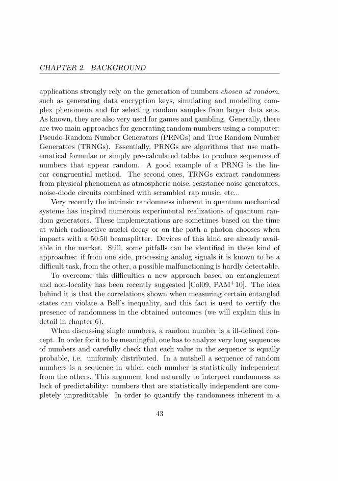
applications strongly rely on the generation of numbers chosen at random,such as generating data encryption keys, simulating and modelling com-plex phenomena and for selecting random samples from larger data sets.As known, they are also very used for games and gambling. Generally, thereare two main approaches for generating random numbers using a computer:Pseudo-Random Number Generators (PRNGs) and True Random NumberGenerators (TRNGs). Essentially, PRNGs are algorithms that use math-ematical formulae or simply pre-calculated tables to produce sequences ofnumbers that appear random. A good example of a PRNG is the lin-ear congruential method. The second ones, TRNGs extract randomnessfrom physical phenomena as atmospheric noise, resistance noise generators,noise-diode circuits combined with scrambled rap music, etc...

Very recently the intrinsic randomness inherent in quantum mechanicalsystems has inspired numerous experimental realizations of quantum ran-dom generators. These implementations are sometimes based on the timeat which radioactive nuclei decay or on the path a photon chooses whenimpacts with a 50:50 beamsplitter. Devices of this kind are already avail-able in the market. Still, some pitfalls can be identified in these kind ofapproaches: if from one side, processing analog signals it is known to be adifficult task, from the other, a possible malfunctioning is hardly detectable.

To overcome this difficulties a new approach based on entanglementand non-locality has been recently suggested [Col09, PAM+10]. The ideabehind it is that the correlations shown when measuring certain entangledstates can violate a Bell’s inequality, and this fact is used to certify thepresence of randomness in the obtained outcomes (we will explain this indetail in chapter 6).

When discussing single numbers, a random number is a ill-defined con-cept. In order for it to be meaningful, one has to analyze very long sequencesof numbers and carefully check that each value in the sequence is equallyprobable, i.e. uniformly distributed. In a nutshell a sequence of randomnumbers is a sequence in which each number is statistically independentfrom the others. This argument lead naturally to interpret randomness aslack of predictability: numbers that are statistically independent are com-pletely unpredictable. In order to quantify the randomness inherent in a

43

2.5. RANDOMNESS

given process the concept of predictability hence turns out to be useful.

2.5.1 Definitions

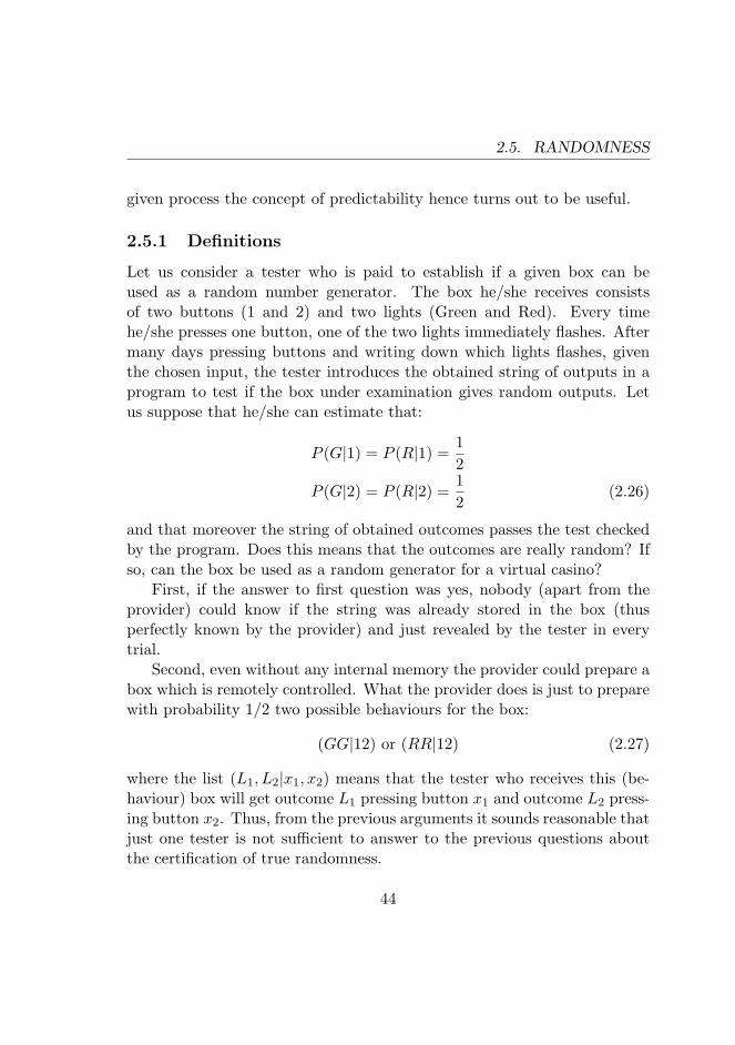
Let us consider a tester who is paid to establish if a given box can beused as a random number generator. The box he/she receives consistsof two buttons (1 and 2) and two lights (Green and Red). Every timehe/she presses one button, one of the two lights immediately flashes. Aftermany days pressing buttons and writing down which lights flashes, giventhe chosen input, the tester introduces the obtained string of outputs in aprogram to test if the box under examination gives random outputs. Letus suppose that he/she can estimate that:

P (G|1) = P (R|1) =12

P (G|2) = P (R|2) =12

(2.26)

and that moreover the string of obtained outcomes passes the test checkedby the program. Does this means that the outcomes are really random? Ifso, can the box be used as a random generator for a virtual casino?

First, if the answer to first question was yes, nobody (apart from theprovider) could know if the string was already stored in the box (thusperfectly known by the provider) and just revealed by the tester in everytrial.

Second, even without any internal memory the provider could prepare abox which is remotely controlled. What the provider does is just to preparewith probability 1/2 two possible behaviours for the box:

(GG|12) or (RR|12) (2.27)

where the list (L1, L2|x1, x2) means that the tester who receives this (be-haviour) box will get outcome L1 pressing button x1 and outcome L2 press-ing button x2. Thus, from the previous arguments it sounds reasonable thatjust one tester is not sufficient to answer to the previous questions aboutthe certification of true randomness.

44


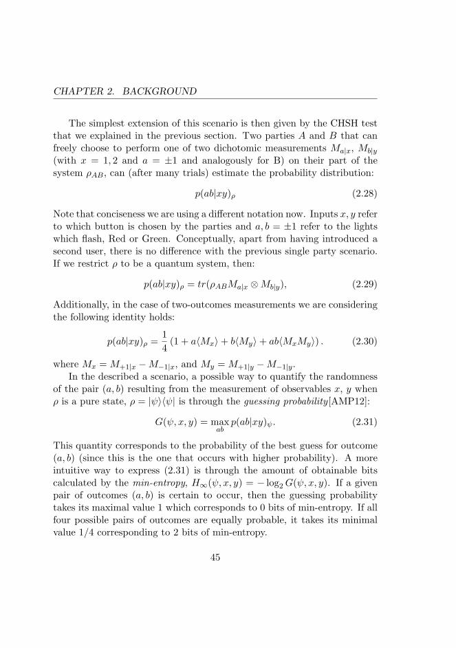
The simplest extension of this scenario is then given by the CHSH testthat we explained in the previous section. Two parties A and B that canfreely choose to perform one of two dichotomic measurements Ma|x, Mb|y(with x = 1, 2 and a = ±1 and analogously for B) on their part of thesystem ρAB, can (after many trials) estimate the probability distribution:

p(ab|xy)ρ (2.28)

Note that conciseness we are using a different notation now. Inputs x, y referto which button is chosen by the parties and a, b = ±1 refer to the lightswhich flash, Red or Green. Conceptually, apart from having introduced asecond user, there is no difference with the previous single party scenario.If we restrict ρ to be a quantum system, then:

p(ab|xy)ρ = tr(ρABMa|x ⊗Mb|y), (2.29)

Additionally, in the case of two-outcomes measurements we are consideringthe following identity holds:

p(ab|xy)ρ =14

(1 + a〈Mx〉+ b〈My〉+ ab〈MxMy〉) . (2.30)

where Mx = M+1|x −M−1|x, and My = M+1|y −M−1|y.In the described a scenario, a possible way to quantify the randomness

of the pair (a, b) resulting from the measurement of observables x, y whenρ is a pure state, ρ = |ψ〉〈ψ| is through the guessing probability [AMP12]:

G(ψ, x, y) = maxab

p(ab|xy)ψ. (2.31)

This quantity corresponds to the probability of the best guess for outcome(a, b) (since this is the one that occurs with higher probability). A moreintuitive way to express (2.31) is through the amount of obtainable bitscalculated by the min-entropy, H∞(ψ, x, y) = − log2G(ψ, x, y). If a givenpair of outcomes (a, b) is certain to occur, then the guessing probabilitytakes its maximal value 1 which corresponds to 0 bits of min-entropy. If allfour possible pairs of outcomes are equally probable, it takes its minimalvalue 1/4 corresponding to 2 bits of min-entropy.

45

2.5. RANDOMNESS

If system ρAB is in a mixed state, the maximization runs over all thepure-state decompositions as follows:

G(ρ, x, y) = maxqm,ψm

∑qmG(ψm, x, y) (2.32)

where ρ =∑

m qm|ψm〉〈ψm|.The definitions given so far are both state dependent and as we will see

can lead to an unwanted incongruence. To overcome that a more generaldefinition can be given which is independent from its quantum realization:

G(P, x, y) = max{ρ,M}7→P

G(ρ, x, y) (2.33)

where {ρ,M} is any quantum realization that is P-compatible, namelyP = tr(ρM) and M = Ma|x ⊗Mb|y. Similarly, a realization-independentguessing probability can be defined for the single party G(P, x) whose min-entropy can vary between 0 and 1. Note that in the previous definitionsno assumption is made about the dimension of the Hilbert space on whichρ and M are defined. This approach is the key idea behind the deviceindependent scenario paradigm.

2.5.2 Link between Randomness and Non-locality

A probability distribution is said local deterministic if every outcome ob-tained locally by the parties is generated deterministically by the value ofthe chosen input. If a measurement v (w) is made by party A (B) thena = f(v) (b = g(y)), where f(g) is a deterministic function of the input v(w). Note that due to the no-signalling condition the output of the partiescan just depend on the local choice of their input. It is thus clear that theguessing probability is equal to 1 in this case. Interestingly this is true forany local distribution.

As proven by Fine [Fin82], every local distribution can be written as aconvex combination of local deterministic distributions (see Appendix D).It is a trivial exercise to find a pure-state (and measurement) representationthat give deterministic outcomes. Thus, each term G(ψm, x, y) appearing

46


in eq. (2.32) is equal to 1 and together with∑

m qm = 1 this implies thatthe guessing probability G(P, x, y) is equal to 1 for any local distribution.Analogously in order for the min-entropy H∞(P, x, y) to be different from0 the probability distribution in exam has to violate a Bell’s inequality(see Appendix D). Thus, a violation of a Bell’s inequality is a necessarycondition for H∞(P, x, y) > 0.

In the following we provide some example to clarify the definitions givenabove. Consider the following probability distribution:

p(ab|xy) =14∀a, b. (2.34)

In what follows, we study different quantum realizations of it. A first wayto fulfil (2.34) is by measuring the maximally entangled state, ψ = (|00〉+|11〉)/

√2 choosing Ax = σx and By = σz. Since ψ is a pure state definition

(2.31) can be used, which gives H∞(ψ, xy) = 2 bits. An alternative way tofulfil (2.34) is by measuring the state ρ = (|00〉〈00|+ |11〉〈11|)/2) with thesame observables Ax, By defined above. Since the state is mixed, definition(2.32) must be used. A straightforward calculation shows that under theprevious decomposition of ρ the value H∞(ρ, xy) = 1 bit is obtained. Notethat one could in principle look for better decompositions of ρ which couldgive H∞(ρ, xy) < 1.

Let us consider a new example. Let p(ab|xy) be the distribution arisingby measuring the maximally entangled state, ψ = (|00〉 + |11〉)/

√2 with

A1 = B1 = σz and A2 = B2 = σx. The choice of settings (1, 2) could inprinciple contain some randomness since the distribution p(ab|12) is equal to1/4 for each a, b. But, it is immediately observed that the whole probabilitydistribution derived in this way does not violate the CHSH inequality (2.19).In fact, there must exist a separable state and some measurements repro-ducing the whole distribution. The guessing probability for this quantumrealization is equal to 1 even for the input’s choice (1, 2) ( H∞(P, 12) = 0).In fact, the separable state and measurements which accomplish that arethe following:

ρAB =14

1∑ij=0

(|ij〉〈ij|A ⊗ |ij〉〈ij|B) (2.35)

47

2.5. RANDOMNESS

A1 = B1 = σz ⊗ I, A2 = B2 = I⊗σx. (2.36)

All these examples show how, given a probability distribution p(ab|xy),different quantum realizations lead to different values of the guessing prob-ability. The realization-independent definition (2.33) avoids all these incon-sistencies.

48

Chapter 3

Can bipartite classicalinformation resources beactivated?

Non-additivity is one of the distinctive traits of Quantum Information The-ory: the combined use of quantum objects may be more advantageous thanthe sum of their individual uses. Non-additivity effects have been proven,for example, for quantum channel capacities, entanglement distillation orstate estimation. In this chapter we consider whether non-additivity ef-fects can also be found in Classical Information Theory. We work in thesecret-key agreement scenario in which two honest parties, having accessto correlated classical data that are also correlated to an eavesdropper,aim at distilling a secret key. Exploiting the analogies between the entan-glement and the secret-key agreement scenario, we show that correlationswith (conjectured) bound information become secret-key distillable whencombined.

49

Introduction

Classical communication systems are governed by classical information the-ory, a vast discipline whose birth coincides with a seminal paper of ClaudeShannon [Sha48]. Among his contributions, Shannon introduced the con-cept of channel capacity, which quantifies the maximum communicationrate that can be achieved over a classical channel. One key feature of thechannel capacity is its additivity: the total capacity of several channels usedin parallel is simply given by the sum of their individual capacities. Thisfact implies thus that the channel capacity completely specifies channel’sability to convey classical information.

Moving to the quantum domain, the quantum channel capacity capturesthe ability of a quantum channel to transmit quantum information. Smithand Yard [SY08] proved recently that the quantum capacity is not additive.In particular, they provide examples of two channels with zero quantum ca-pacity that define a channel with strictly positive quantum capacity whencombined. This intriguing quantum effect is known as activation and cangenerally be understood as follows: the combined use of quantum objectscan be more advantageous than the sum of their individual uses. In thelast years, an intense effort has been devoted to the study of non-additivityeffects in Quantum Information Theory. Classical and private communica-tion capacity of quantum channels were later shown not to be additive inRefs [Has09, LWZG09]. Nowadays, non-additivity is considered to be oneof the distinctive traits of Quantum Information Theory.

Before the results by Smith and Yard, however, non-additivity effectshad also been observed in Entanglement Theory in the context of entan-glement distillation. There, one is interested in the problem of whetherpure-state entanglement –pure entanglement in what follows– can be ex-tracted from a given state shared by several observers using local operationsand classical communication (LOCC). In Ref. [SST03], the authors provideexamples of multipartite states that (i) are non-distillable (bound) whenconsidered separately but (ii) define a distillable state when taken together.Moving to the case of two parties, and leaving aside activation-like resultsas those of [HHH99], it remains unproven whether entangled states can

50

CHAPTER 3. CAN BIPARTITE CLASSICAL INFORMATIONRESOURCES BE ACTIVATED?

be activated. There is however some evidence of the existence of pairs ofbound (non-distillable) entangled states that give a distillable state whencombined [SST01, VW02].

In this chapter we are interested in the question of whether non-additivityeffects can be observed in Classical Information Theory. As mentioned,classical channel capacities are known to be additive. Therefore, we moveour considerations to distillation scenarios. In particular, we focus on theclassical secret-key agreement scenario in which two honest parties, havingaccess to correlated random variables, also correlated with an adversary,aim at establishing a secret key by local operations and public communi-cation (LOPC). While the activation of classical resources has been shownin a multipartite key-agreement scenario in [ACM04, PB11], here we con-sider the more natural case of two honest parties. In our study, we exploitthe analogies between the secret-key agreement and entanglement scenarionoted in [GRW02]. Based on the results of [VW02], we provide evidencethat activation effects may be possible in the completely classical bipartitekey-agrement scenario. Our findings, therefore, suggest that the classicalsecret-key rate is non-additive.

This chapter is structured as follows. Section 3.1 introduces the quan-tum scenario, namely the quantum states and the protocol of activation.In section 3.2 we derive their classical analog. Section 3.3 concludes with adiscussion on how our findings are related to other results and conjecturesin the field.

3.1 Quantum Activation

As mentioned, we start by presenting the example of activation of distillableentanglement given in Ref. [VW02]. After introducing the states involvedin this example, we review their distillability properties and the quantumprotocol that attains the activation.

51

3.1. QUANTUM ACTIVATION

3.1.1 Quantum States

States that are invariant under a group of symmetries play a relevant role inthe study of entanglement. The two classes of symmetric states consideredhere are Werner states [Wer89] and the symmetric states of Ref. [VW01,VW02], named in what follows symmetric states for the sake of brevity.

Werner States

Acting on an Hilbert space H = HA ⊗ HB with dimensions dim(HA) =dim(HB) = d, and commuting with all unitaries U ⊗ U , Werner states canbe expressed as:

ρW (p) = pAd

tr(Ad)+ (1− p) Sd

tr(Sd)(3.1)

where Ad = (1 − Πd)/2, Sd = (1 + Πd)/2 are the projector operatorsonto the antisymmetric and symmetric subspaces, Πd is the flip operatorand tr(Ad) = d(d− 1)/2, tr(Sd) = d(d+ 1)/2. It is known that states (3.1)are entangled and NPT iff p > ps = 1/2. Moreover they are distillable,actually 1− distillable, if p > p1d = 3τ/(1 + 3τ), where τ = tr(Ad)/tr(Sd).The states are conjectured to be bound entangled for ps < p ≤ p1d.

Symmetric States

Acting on an Hilbert space H = HA1 ⊗HA2 ⊗HB1 ⊗HB2, the symmetricstates under consideration commute with all unitaries of the form W =(U ⊗ V )A ⊗ (U ⊗ V ∗)B (where V ∗ is the complex conjugate of V ). Thesestates can be represented in a compact form as [VW01]:

σ =4∑i=1

λiPi/tr[Pi]

where P1 = A(1)d ⊗ P

(2)d , P2 = S(1)

d ⊗ P(2)d , P3 = A(1)

d ⊗ (1− Pd)(2), P4 =S(1)d ⊗(1− Pd)(2). Pd and 1−Pd represent the projector onto the maximally

52


entangled state |ψ+d 〉 = 1/

√d∑d

i=1 |ii〉, and its orthogonal complement,respectively. In Ref. [VW02] the authors identify a region in the spaceof parameters λi so that the state σ (i) is bound entangled but (ii) givesa distillable state when combined with a Werner state in the conjecturedregion of bound entanglement. Among all the states with these properties,we focus here on:

σ(q) = qAd

tr(Ad)⊗ Pd + (1− q) Sd

tr(Sd)⊗ (1− Pd)tr(1− Pd)

(3.2)

where q = 1/(d+ 2). This state is a universal activator, in the sense that itdefines a distillable state when combined with any entangled Werner state.It is also relevant for what follows to study the distillability properties ofstates (3.2) for any value of q and d = 3. These states are NPT and 1-distillable for q > 1/5. The latter follows from the fact that in this region,there exist local projections on two-qubit subspaces mapping states (3.2)onto an entangled two-qubit state. The qubit subspaces are spanned by|00〉, |01〉 on Alice’s side and |10〉, |11〉 on Bob’s. Figure 3.1 summarizes themain entanglement properties of these states.

3.1.2 Protocol for Quantum Activation

As already announced, any entangled Werner state, and in particular anyconjectured bound entangled Werner state, gives a distillable state whencombined with the universal activator σ(q) with q = 1/(d + 2), simplydenoted as σ. If initially the two parties are sharing a Werner state ρ actingon H0 = HA0⊗HB0 and a symmetric state σ acting on H1,2 = HA1⊗HA2⊗HB1 ⊗ HB2 , each party applies a projection onto a maximally entangledstates on HA0 ⊗ HA1 and HB0 ⊗ HB1 respectively. The resulting state isan isotropic state ρiso acting on HA2 ⊗HB2 . Recall that isotropic state areU ⊗ U∗ invariant and defined by the convex combination of a maximallyentangled state and white noise, I /d2. One can see that the resultingisotropic state has an overlap with a maximally entangled state, tr(ρisoPd),larger than 1/d for any entangled Werner state. As shown in [HH99], thiscondition is sufficient for distillability.

53

3.2. CLASSICAL ACTIVATION

Figure 3.1: Entanglement properties of Werner, ρW , and symmetric state, σ(q), for thequtrit case (d = 3). In the region between separability and 1-distillability, ρW is NPPTand conjectured bound. The point q = 0.2 represents the extremal value for which statesσ(q) are PPT, thus not distillable. For larger values of q the states are distillable (inparticular, 1-distillable).

3.2 Classical Activation

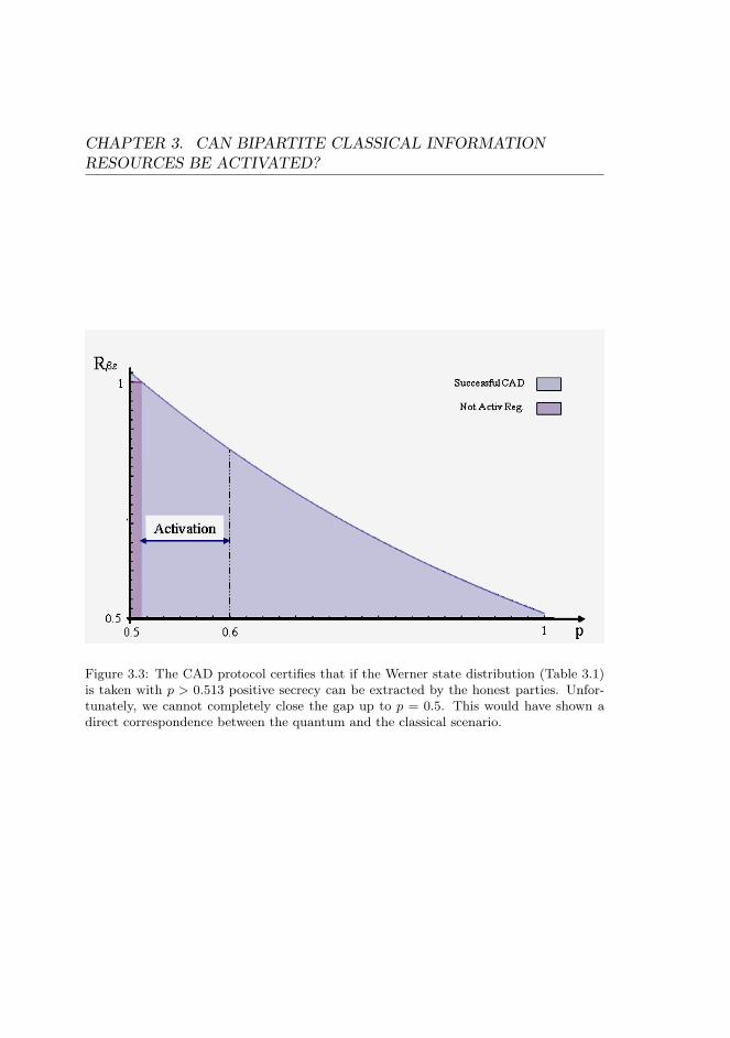
This section presents our main results. Exploiting the analogies betweenthe entanglement and secret-key agreement scenarios, we study whetherit is possible to derive a cryptographic classical analog of the activationof distillable entanglement between bipartite quantum states given aboveRef. [VW02]. We map the involved quantum states onto probability distri-butions and study their secrecy properties. After applying classical distil-lation protocols, we show how the honest parties are able to distill a secretkey from each of the distributions for the same range of parameters as inthe quantum regime (ED > 0). Finally, we introduce a distillation protocolanalogue to the one used for the quantum activation. We prove that thisprotocol activates probability distributions containing conjectured boundinformation, although we cannot completely recover the quantum region.

We first associate probability distributions to all the previous quan-tum states. In order to do so, we purify the initial bipartite noisy quan-tum states ρAB by including an environment, and then map the tripar-

54


tite quantum states |ψABE〉 onto probability distributions by performingsome local measurements, see (2.15). The procedure to choose these mea-surements is always the same: computational bases for the honest parties,and general measurements for Eve. More precisely, denoting by X and Ythe result obtained by Alice and Bob, this effectively projects Eve’s sys-tem onto the pure state |eXY 〉 = 〈XY |ψABE〉 with probability P (XY ) =〈XY |ρAB|XY 〉. Given that, the measurement that Eve applies is the onethat minimizes her error probability when distinguishing the states in theensemble {|eXY 〉, P (XY )}. Note that this choice of measurement may notnecessarily be optimal from Eve’s point of view in terms of the secret corre-lations between Alice and Bob, but it seems a natural choice. This proce-dure is applied to the two family of states, namely Werner and symmetric.Because of the symmetries of these states, the measurements minimizingEve’s error probability can be analytically determined using the results ofRefs [Hel76, EF01].

In order to characterize the secrecy properties of the obtained proba-bility distributions, we compute the intrinsic information when numericallypossible and use AD protocols for distillability. We stress that the con-sidered protocols distill a secret key in the same region of parameters inwhich entanglement distillation was possible for the initial quantum states.Finally, we introduce a quantum-like activation protocol that maps the twoprobability distributions into a new distribution in which Alice and Bobeach have a bit. We then prove that an AD protocol allows distilling asecret key for some value of the parameters in which the initial quantumstates were non-distillable. However, we are unable to close all the gapbetween entanglement and 1-distillability for the Werner state.

3.2.1 Probability Distributions

We map now quantum states to probability distributions through measure-ments on them (as discussed in section 2.3).

55


Werner states distribution

We start by mapping the Werner states of two qutrits onto a probabilitydistribution PXY Z following the recipe explained in the previous section. Inthis way, we get a one-parameter family of probability distributions PXY Z ,(see Table 3.1 for details), which depends just on the same parameter pdefining the initial Werner state (3.1). The resulting distributions are givenin Table 3.1. The indices for Eve’s symbols specify her guess on Alice’s andBob’s symbols or, in other words, if Eve outcome is Z = zij , the mostprobable outcomes for Alice and Bob are X = i and Y = j.

0 1 2

0 λ1 (z00) λ1+λ22

{δZ (z10)

1− δZ (z01)λ1+λ2

2

{δZ (z20)

1− δZ (z02)

1 λ1+λ22

{δZ (z01)

1− δZ (z10)λ1 (z11) λ1+λ2

2

{δZ (z21)

1− δZ (z12)

2 λ1+λ22

{δZ (z02)

1− δZ (z20)λ1+λ2

2

{δZ (z12)

1− δZ (z21)λ1 (z22)

Table 3.1: Tripartite probability distributions derived from Werner states (3.1). Theparameters in the table are as follows: λ1 = (1 − p)/6, λ2 = p/3 and δZ = (

√λ1 −√

λ2)2/(2(λ1 + λ2)). Rows (columns) represent Alice’s (Bob’s) symbols. Eve’s symbolsare shown in parenthesis. For example, the cell (X = 0, Y = 1) shows that whenever Aliceand Bob get (0,1) (which happen with probability (λ1 +λ2)/2), Eve correctly guesses thesymbol z01 with probability 1− δZ , and makes an error (symbol z10) with probability δZ .

As done for entanglement, we now characterize these distributions interms of their secret correlations. Recall that for the quantum case andqutrits, the state was entangled for p > ps = 1/2 and conjectured non-distillable for p ≤ p1d = 3/5. As we show next, the same values appear forthe analogous classical distributions. Concerning the point ps, we compute

56


the intrinsic information of the distributions in Table 3.1 by numerical opti-mization over all possible channels by Eve. Of course, one can never excludethe existence of local minima and, therefore, that the intrinsic information isstrictly smaller than what numerically obtained. One may wonder why thiscomputation is necessary. For instance, at the point p = ps the quantumstate is separable and, then, it is known that there exists a measurementby Eve such that the intrinsic information between Alice and Bob is zerofor all measurements. Note however that in terms of intrinsic information,the optimal measurement by Eve is the one that prepares on Alice andBob the ensemble of product states compatible with the separable stateAlice and Bob share. This measurement is not necessarily the same as theone minimizing Eve’s error probability when Alice and Bob measure in thecomputational bases. The same applies to the entanglement region. Whilethere are measurements such that Alice and Bob share secret correlationsno matter which measurement Eve performs, these measurements are noton the computational bases.

Using the numerical insight, we find a conjectured optimal channel thatreproduces the numerical results. The optimal channel gives zero intrinsicinformation exactly at the point p = ps. It maps Eve’s symbols zii onto zijwith i 6= j with equal probability (i, j = 0, 1, 2). Its easy form leads to thefollowing analytical expression for I(X;Y ↓ Z):

I(X;Y ↓ Z) = − log(1− x2)− x log

(1 + x

1− x

√τ − 2xτ + 2x

)+

τ

4log (τ2 − 4x2) +

(1− τ

2

)log(2− τ)

where τ = 1 + p, x =√

2p(1− p). Figure 3.2 shows the behavior of thisquantity in the region of interest.

Moving to the distillability properties, we study AD protocols and iden-tify a value of p for which positive secret-key rate can be obtained by thetwo honest parties through these protocols. The considered protocol is the

57


Figure 3.2: Behaviour of the intrinsic information for the PXY Z relative to the Wernerstate. Note that: i) I(X;Y ↓ Z) is equal to 0 at point p = 0.5 which corresponds to thelast point of separability for the Werner state; ii) I(X;Y ↓ Z) is strictly positive at pointp = 0.6 which corresponds to the extreme value of p for which it is 1-copy distillable.

quantum analogue of the quantum one and uses a binaryzation. Alice andBob first discard one (but the same) of their symbols. Then, one of theparties, say Bob, applies a local permutation to his symbols. For example,if they agreed on discarding symbol 2, then Bob applies 0 ↔ 1. Alice andBob now apply AD to the resulting two-bit distribution. This distributionis shown in Table 3.2.

From the obtained table, it is possible to estimate the dependence ofBob’s and Eve’s errors on the size of the blocks used for AD, denoted by N .Recall that in the case of bits the protocols works as follows: Alice generatesa random bit ζ and chooses N symbols a from her list of data. She thensends to Bob the information about these symbols and the vector a suchthat ai ⊕ ai = ζ,∀i. Bob takes the symbols in his list corresponding tothose chosen by Alice, b, and accepts only when χ = bi⊕ ai,∀i. Bob’s errorprobability βN is now easy to compute. Denote by β the error probabilityin the initial two-bit probability distribution, β = P (X 6= Y ) = 2λ1/(3λ1 +λ2). Bob accepts a bit whenever either all his N symbols are identical to

58


those of Alice, which happens with probability (1− β)N , or all his symbolsare different, whose probability is βN . Thus, the probability of accepting awrong bit conditioned on acceptance is given by:

βN =βN

βN + (1− β)N6

(β

1− β

)N. (3.3)

The upper bound becomes tight in the limit N →∞.

0 1

0 λ1+λ22

{δZ (z11)

1− δZ (z00)λ1 (z01)

1 λ1 (z10) λ1+λ22

{δZ (z00)

1− δZ (z11)

Table 3.2: Two-bit distribution resulting from projecting the initial distribution of Ta-ble 3.1 on the space X,Y = 0, 1 and after Bob permutes his symbol. For the sakeof clarity, we apply a permutation also on the second index of Eve’s symbols, that iszij → zi1−j . All the terms in the table should be normalized by a factor 3λ1 + λ2.

We now move to the estimation of Eve’s error εN . As her informationis probabilistic, there is always a non-zero probability that she makes amistake. For the estimation we compute a lower bound on the error givenby all the cases in which the N symbols observed by Eve do not provideher any information about the value of the bit generated by Alice. In thecomputation, it is simpler to use Eve’s probabilities conditioned on the factthat Alice and Bob have made no mistake after AD (which means that nomistake has occurred for any of the N symbols). Or in other words, we onlyconsider the terms in the diagonal of Table 3.2. This does not make anydifference for what follows as in the limit N → ∞ the probability of Bobaccepting a wrong symbol goes to zero. After Bob’s acceptance, Eve knows

59


that the actual string a used by Alice is either equal to a (the one sent onthe public channel) when ζ = 0, or a′ (the permuted one, that is, a′i = 1−ai)when ζ = 1. Clearly, all the events in which the N symbols observed byEve, Z(i), are such that P (Z(1).. Z(N)|a = a) = P (Z(1).. Z(N)|a = a′) donot give her any information about ζ. In these cases, Eve has to randomlyguess Alice’s symbol and makes an error with probability 1/2. Due to thesymmetry in the diagonal of Table 3.2, that is, P (Z = z00|X = 0) = P (Z =z11 = 1|X = 1) and P (Z = z11|X = 0) = P (Z = z00|X = 1), all the eventswhere Eve has exactly N/2 of her symbols equal to z00 and N/2 equal to z11

satisfy the previous condition and, thus, contribute to her error. Countingall the possible ways of distributing these cases leads to the following lowerbound on Eve’s error probability [GW99]:

εN >12

(NN/2

)δN/2Z (1− δZ)N/2 (3.4)

where δZ is the probability for Eve to guess wrongly conditioned on thosecases in which Alice and Bob’s symbols coincide (this value is made ex-plicit in the caption of Figure 3.1). The asymptotic behavior of (3.4), afterapplying the Stirling’s approximation (n!)2 ' (2n)!/22n and expanding thebinomial coefficient can be expressed as:

εN > c(2√δZ(1− δZ))N , (3.5)

with c being a positive constant.By comparing Eqs. (3.3) and (3.5) one concludes that whenever

β

1− β< 2√δZ(1− δZ) (3.6)

key distillation is possible. This follows from the fact that, if this conditionholds, Bob’s error is exponentially smaller than Eve’s with N . This in turnimplies that it is possible to choose a value of N such that Alice-Bob mutualinformation is larger than Alice-Eve and one-way distillation techniques candistill a secret key (we show this in appendix A ). From (3.5) one gets thatAD works whenever p > 3/5, as for 1-distillability in the quantum case.

60


Before concluding this part, we would like to mention that the same rangeof parameters for distillation is obtained if one applies the generalized ADprotocol of Ref. [AGS03].

Symmetric states distribution

We apply the same machinery to the symmetric states σ(q). Again, thesymmetries of the states allow the explicit computation of the measurementby Eve minimizing her error probability for any value of q. The obtaineddistributions, denoted by QX1,Y 1,X2,Y 2,Z , is significantly more complex andshown in Appendix A. It consists of two trits for Alice, (X1, X2) and twotrits for Bob, (X2, Y2), while Eve’s variable can take 63 possible values. It isnow much harder to estimate the secrecy properties of the distribution. Forinstance, we did not make any attempt to compute the intrinsic information.However, we are able to show that Alice and Bob can distill a secret keywhenever q > 1/5 as in the quantum regime.

To simplify our task, we exploit again the concept of binaryzation. In-spired by the quantum projections used for the distillation of σ(q), Aliceand Bob select two outcomes on each side, namely 00, 01 for Alice and 10, 11for Bob. The obtained two-bit distribution is shown in Table 3.3.

They apply the standard bit AD protocol to this distribution. As before,Bob’s error can be easily computed, getting the same as in Eq. (3.3), butnow with β equal to 3(1−q)/(5+11q). The estimation of Eve’s error is muchmore cumbersome. As above, the main idea is to derive a lower bound onit based on those instances in which Eve’s symbols do not provide her anyinformation about the symbol ζ Alice used for AD. Again, one can restrictthe analysis to the terms in the diagonal of Table 3.3. The main differencein comparison with the simple case discussed above is the larger number ofsymbols for Eve. However, given the symmetry of the distribution 3.3 it is

61


0 [10] 1 [11]

0 [00] 1+7q5+11q

PG (z0100)

PL (z0111)

PL (z0122)

PB (z1000)

PH (z1011)

PH (z1022)

3(1−q)2(5+11q)

1/2 (z0101)

1/2 (z1001)

1 [01] 3(1−q)2(5+11q)

1/2 (z0110)

1/2 (z1010)1+7q5+11q

PL (z0100)

PG (z0111)

PL (z0122)

PH (z1000)

PB (z1011)

PH (z1022)

Table 3.3: Two-bit distribution obtained as a result of the binaryzation applied toQX1,Y 1,X2,Y 2,Z . Note that we have relabeled the old symbols (shown in square brakets)

by 0 and 1, in the following we use X, Y to refer to them. The parameters in the tableare as follows: α =

p8q/(1 + 7q) and γ =

p(1− q)/(2(1 + 7q)), PG = (α + 2γ)2/6,

PB = (−α+ 2γ)2/6, PL = (α− γ)2/6, PH = (α+ γ)2/6.

62


enough to consider Eve’s symbols pair-wise:

P (Z = z0100|XY = 00) = P (Z = z0111|XY = 11) = δ1

P (Z = z0100|XY = 11) = P (Z = z0111|XY = 00) = η1

P (Z = z1000|XY = 00) = P (Z = z1011|XY = 11) = δ2

P (Z = z1000|XY = 11) = P (Z = z1011|XY = 00) = η2

where we have used X, Y to denote the re-labeling of Alice and Bob’ssymbols. Note that the last two subindexes of Eve’s symbols are thosethat give her information about Alice’s (and Bob’s) symbol. Symbols z∗∗22

give her no information about Alice’s symbols, so we sum them, their totalprobability being δ3. Given the public string aN , one can see that all thosecases for which Eve has the same number n1 of z0100 and z0111 and the samenumber n2 of z1000 and z1011, with N = 2n1 + 2n2 + 2n3 and where 2n3 isthe total number of symbols z∗∗22, contribute to her error. Thus, countingall these cases leads to the following lower bound on Eve’s error:

εN >12

∑n1,n2,n3

N !(2n1)!(2n2)!(2n3)!

(2√δ1η1

)2n1(

2√δ2η2

)2n2

(δ3)2n3

(3.7)where δi and ηi are the probabilities shown above but normalized (sinceas already stated we are considering the asymptotic case). After Stirling’sapproximation and summing eq. (3.7) the following compact form is ob-tained:

εN > c(

2√δ1η1 + 2

√δ2η2 + δ3

)Nwith c being a positive constant. Comparing the scaling of the errors, onehas that AD works whenever

β

1− β< 2√δ1η1 + 2

√δ2η2 + δ3 (3.8)

63


where the right hand side is equal to (α+ γ)2/3 (the values of α and γ arereported in the caption of Table 3.3). Simple algebra shows that eq. (3.8)is satisfied whenever q > q = 0.2, as announced.

3.2.2 Protocol for Classsical Activation

Inspired by the quantum activation example of Ref. [VW02], we considerthe following classical protocol. Alice and Bob have access to the tritsX and Y , whose correlations are described by PXY Z , and the two trits(X1, X2) and (Y1, Y2) correlated according to QX1,Y 1,X2,Y 2,Z . Alice (Bob)keeps X2 (Y2), and only X2 (Y2), whenever X = X1 (Y = Y1); otherwisethey discard all the symbols. This filtering projects the initial probabilityinto a slightly simpler two-trit distribution. The new probability distribu-tion Q∗(X2, Y2, E) reads:

Q∗(X2, Y2, E) =2∑

x,y=0

P (X = x, Y = y, Z)Q(X1 = x, Y1 = y,X2, Y2, Z)

(3.9)where E = [Z, Z] is the collection of Eve’s ymbols. Finally Alice and Bobbinaryze their symbols by discarding one of the three values (the same forboth), say 2. The resulting distribution is shown in Table 3.4.

As above, we use AD protocols to estimate the value of p for whichAlice and Bob can extract a positive secret key rate if they are sharingpairs of bits distributed according to Table 3.4. We are able to prove thatwhenever p > pc ' 0.513 an AD protocol allows distilling a secret key fromthe distribution in Table 3.4 and, thus, a form of activation is possible.Unfortunately, we are unable to reach the point p = 0.5, as in the quantumscenario. However, our analysis suggests that the secret key rate is non-additive for some values of p. In the following we summarize the key stepsleading to this result.

As mentioned, the values of interest for PXY Z and QX1,Y 1,X2,Y 2,Z are,0.5 < p 6 0.6 and q = 0.2, respectively. The distribution Q∗(X2, Y2, E)resulting from the local filtering by the honest parties depends on the pa-rameter p. In order to estimate Eve’s error we follow a similar argument


Figure 3.3: The CAD protocol certifies that if the Werner state distribution (Table 3.1)is taken with p > 0.513 positive secrecy can be extracted by the honest parties. Unfor-tunately, we cannot completely close the gap up to p = 0.5. This would have shown adirect correspondence between the quantum and the classical scenario.


0 1

0

λ1(1−q)72cN

2/3 (zii, zii00)

1/6 (zii, zii11)

1/6 (zii, zii22)

λ1(1−q)48cN

1 (z00, z0001)

1 (z11, z1101)

1 (z22, z2201)

ΛsN

δZPG + (1− δZ)PB (zts, zst00)

δZPL + (1− δZ)PH (zts, zst11)


δZPB + (1− δZ)PG (zts, zts00)

δZPH + (1− δZ)PL (zts, zts11)


δZPB + (1− δZ)PG (zst, zst00)

δZPH + (1− δZ)PL (zst, zst11)


δZPG + (1− δZ)PB (zst, zts00)

δZPL + (1− δZ)PH (zst, zts11)


Λ(1−q)96cN

1/2 (z01, z0101)

1/2 (z01, z1001)

1/2 (z10, z0101)

1/2 (z10, z1001)

1/2 (z02, z0201)

1/2 (z02, z2001)

1/2 (z20, z0201)

1/2 (z20, z2001)

1/2 (z12, z1201)

1/2 (z12, z2101)

1/2 (z21, z1201)

1/2 (z21, z2101)

1

λ1(1−q)48cN

1 (z00, z0010)

1 (z11, z1110)

1 (z22, z2210)

λ1(1−q)72cN

1/6 (zii, zii00)

2/3 (zii, zii11)

1/6 (zii, zii22)

Λ(1−q)96cN

1/2 (z01, z0110)

1/2 (z01, z1010)

1/2 (z10, z0110)

1/2 (z10, z1010)

1/2 (z02, z0210)

1/2 (z02, z2010)

1/2 (z20, z0210)

1/2 (z20, z2010)

1/2 (z12, z1210)

1/2 (z12, z2110)

1/2 (z21, z1210)

1/2 (z21, z2110)

ΛsN


δZPG + (1− δZ)PB (zts, zst11)



δZPB + (1− δZ)PG (zts, zts11)



δZPB + (1− δZ)PG (zst, zst11)



δZPG + (1− δZ)PB (zst, zts11)


Table 3.4: The initial probability distributions PXY Z and QX1,Y 1,X2,Y 2,Z are mappedthrough the classical protocol to the new probability distribution Q∗(X2, Y2, E) shownabove. From it we derive the minimum value of p for which positive secret key can beextracted by A and B. The parameters appearing above are expressed as a function of pand q: Λ = (λ1+λ2)/2, cN = (λ1+λ2)(5+11q)/48+5λ1(1−q)/24, sN = (1+7q)/(144cN ),i, s, t = 0, 1, 2 with s 6= t and s < t. The optimal q corresponds to 1/5.


as for QX1,Y 1,X2,Y 2,Z , now adapted to this slightly more complex case. De-spite the big amount of symbols on Eve’s side (see Table 3.4), the symmetryin the distribution leads to six main classes that are relevant for the ADanalysis (appendix A further clarifies this point). These arguments lead tothe following bound on Eve’s error:

εN >12

∑n1,n2...n6

N !(2n1)! . . . (2n6)!

(6√δ1 η1

)2n1

. . .(

6√δ5 η5

)2n5

δ2n66

(3.10)where

∑6i=1 2ni = N . Note that as before the terms δiηi with i = 1 . . . 5

take into account those cases in which Eve has ni symbols that coincidewith the public string sent by Alice and ni symbols that are opposite tothose appearing in the public string. The last term, δ6, as before, refers tothe sum of probabilities for which Eve has no information at all (see detailsin appendix A). In the asymptotic case we are treating here, Eq. (3.10)converges to a multinomial distribution, namely:

εN > c(

6(√

δ1 η1 + . . .√δ5 η5

)+ δ6

)N(3.11)

with c being a positive constant. Bob’s error is much easier to compute,getting β = (3λ1 + λ2)(1 − q)/(16cN ). Putting these two terms together,we have that the AD protocols works whenever:

β

1− β< 6

(√δ1 η1 + . . .

√δ5 η5

)+ δ6 (3.12)

Figure 3.3 shows the ratio between the left hand side and the right handside, Rβε, as a function of the parameter p. As above, whenever Rβε < 1,the AD protocol succeeds. The point at which Rβε = 1 corresponds top = 0.513, as already announced.

3.3 Conclusions

Non-additivity is an ubiquitous phenomenon in Quantum Information The-ory due to the presence of entanglement. In this work, we provide some

67

3.3. CONCLUSIONS

evidence for the existence of similar effects for secret classical correlations.Exploiting the analogies between the entanglement and secret-key agree-ment scenario, we have shown that two classical distributions from whichno secrecy can be extracted by AD protocols can lead to a positive secretkey rate when combined.

The evidence we provide is somehow similar to the conjectured exampleof activation for bipartite entangled states. Note however that, in the quan-tum case, one of the two states is provably bound. As mentioned severaltimes, it could well happen that one, or even the two probability distri-butions considered here are key-distillable. Indeed, there exist examples ofbound entangled states from which one can obtain probability distributionswith positive secret-key rate [HHHO05]. Note however that all the knownexamples of bound entangled states with non-zero privacy are based onthe existence of ancillary systems on the honest parties, known as shields,that prevent Eve from having the purification of the systems Alice and Bobmeasure to construct the key. If any of the probability distributions con-structed here were key distillable, they would constitute a novel exampleof secret correlations from a bound entangled state that does not fit in theconstruction of [HHHO05].

68

Chapter 4

Superactivation,unlockability, and secrecydistribution of boundinformation

Bound information, a cryptographic classical analogue of bound entangle-ment, is defined as secret classical correlations that despite containing se-crecy, do not allow separate parties to extract it. The existence of this kindof correlations was conjectured in the bipartite case and later shown in themultipartite case. In this chapter, we provide a new example of boundinformation in the four-partite scenario. Later, we prove that this boundinformation shares the same properties as the original quantum state fromwhich it is derived, namely, superactivation in a finite-copy scenario andunlockability. We also show that the bound entangled state in exam, andalso the derived bound information, can be used to distribute multipartitepure-state entanglement and secret correlations, respectively.

69

4.1. INTRODUCTION

4.1 Introduction

Following the analogy between entanglement and secret-key agreement,Gisin and Wolf conjectured and gave evidence for the existence, in the bi-partite scenario, of a classical analog of bound entanglement, the so-calledbound information. Despite firstly defined as a bipartite concept, the boundinformation can unambiguously generalised to more honest parties plus aneavesdropper. In the four partite case, for example, P (A,B,C,D, E) it issaid to contain bound information if i) no pair of honest parties, even withthe help of the other ones, can generate a secret key from any instances ofP (A,B,C,D, E), ii) P (ABCDE) cannot be distributed by LOPC opera-tions.

Remarkably, while only conjectured in the bipartite case, a proof ofbound information was provided in the three-partite case. This result waspossible due to the possibility to consider different bipartitions for which theintrinsic information is zero (see below). The probability distribution wasderived directly by measuring a bound entangled state in the computationalbasis of the separated parties and then shown to be bound by means ofclassical tools. Additionally it was proved that such a bound informationcould be activated in the asymptotic case of many copies, analogously tothe entanglement scenario.

In this chapter we provide a novel example of multipartite bound infor-mation, which in contrast with the previous example, can be activated inthe finite copy scenario. As a consequence of that, no advantage distillationprotocols are needed to show the positivity of the key rate of the combineddistributiions. Additionally, we show that as for the quantum case, theobtained bound information is shown to be unlockable. All these findingsare based on the interesting properties of the Smolin state introduced inRef. [Smo01] that we could translate to the classical scenario.

Finally, we provide another useful feature of the correlations in exam todistribute pure-state entanglement and multipartite sbits. In the quantumscenario, we show that the tripartite GHZ state can be extended to the four-partite GHZ state using LOCC, given that a four-partite bound entangledstate is shared among parties. As expected, we show this to be true for the

70

CHAPTER 4. SUPERACTIVATION, UNLOCKABILITY, ANDSECRECY DISTRIBUTION OF BOUND INFORMATION

classical analogue too: when bound information is shared by four parties,an sbit of three parties can be distributed over the four parties using LOPC.

This chapter is organized as follows. Sec. 4.2, briefly defines and reviewsthe properties of the Smolin states. In Sec. 4.3, the existence of boundinformation is shown and the properties of unlockability and superactivationare translated from the quantum to the classical case. In Sec. 4.4, itis shown that bound entangled state (bound information) together withLOCC (LOPC) can be used to extend GHZ states (sbits) from three tofour parties.

4.2 The Smolin State

Let us first briefly review the properties of the Smolin state presented inRef. [Smo01]. The Smolin state is a four-partite bound entangled state,shared by, say Alice, Bob, Clare and David:

ρABCD =14

∑i

|ψi〉AB〈ψi| ⊗ |ψi〉CD〈ψi|, (4.1)

where |ψ1〉 = (|00〉 + |11〉)/√

2, |ψ2〉 = (|00〉 − |11〉)/√

2, |ψ3〉 = (|01〉 +|10〉)/

√2, and |ψ4〉 = (|01〉 − |10〉)/

√2. This state has been exploited

to derive intriguing effects of bound entanglement such as the unlockabilityand the superactivation in a finite-copy scenario [Smo01]. Let us summarizethe properties in the following.

i) Invariance under permutations. The state is symmetric under anyexchange of parties, i.e. ρABCD = ρABDC = ρADBC .

ii) Undistillability. Looking at the bipartite splitting AB : CD in thestate in Eq. (4.1), it is clear that the state is separable across the cut.Then, from the property i), it follows that the state is separable inall bipartitions across two parties versus the others, such as AC : BDand AD : BC. This already shows that no pair of parties can distillentanglement, and therefore the state is undistillable.

71

4.2. THE SMOLIN STATE

iii) Unlockability. An important property of the state is the unlockabilityof entanglement. This can be seen when two parties among the fourjoin together and apply collective operations to discriminate amongthe four Bell states. Announcing the measurement outcome, the twojoined parties can allow the other two parties to know which Bell statethey share. Consequently, applying local unitaries depending on theannounced outcome, they can finally distill the Bell state |ψ1〉. Thisshows that the Smolin state is entangled, and also bound entangledtogether with the property ii).

4.2.1 Quantum superactivation with finite copies

As said, one of the intriguing effects shown in entanglement theory is thatof activation of bound entangled states. It is based on the fact that thecombination of two (or more) bound entangled states, thus per se non-distillable, can be brought to a state which is indeed distillable. The Smolinstate was in particular exploited to show a stronger version of such an effect.Termed superactivation, it refers to the superadditivity of the distillableentanglement: given two mixed states ρ1, ρ2, ED(ρ1 ⊗ ρ2) > 0 despite thefact that ED(ρ1) = ED(ρ2) = 0. This was shown in Ref. [SST03] withoutthe restrictions of the earlier types of activation of bound entanglement[DC00]. The quantum activation protocol works as follows. Suppose that,now including a fifth party, Elena, two copies of the Smolin state are sharedby the five parties in the following way,

ρA1C1B1D ⊗ ρA2B2C2E , (4.2)

where the first and the second copies are labeled. Then, David and Elenadistill an ebit, applying the following protocol, see also Fig. 4.1. First, Aliceteleports her qubit state of A2 to Clare sacrificing the unknown Bell stateshared between A1 and C1. Clare is then with two qubits C

′1 and C2 where

C′1 is in the teleported state from A2. Next, Bob teleports his qubit state

of B2 to D using the unknown Bell state shared between B1 and D. Then,David is now with D

′in the teleported state from B2. Finally, due to the

72


Alice Bob

DavidClare

Elena

2A

1A

1C

1B

D

2B

E2C

Alice Bob

DavidClare

Elena

'1C

1B

D

2B

E2C

Alice Bob

DavidClare

Elena

'1C 'D

E

2C

(I)(II)

(III) (IV)Alice Bob

DavidClare

Elena

'D

E

Figure 4.1: The activation protocol for both the quantum and classical scenarios is shown.For the quantum scenario, two Smolin states ρA1C1B1D and ρA2B2C2E are drawn withthe dashed and solid lines, respectively. For the classical scenario, the Smolin states aresimply replaced with the bound information in (4.5). In both cases, the first step in theprotocol (shown in I→II) is that Alice teleports her state in the system A2 to C1 using thecorrelation between A1C1. In the second step (shown in II→III), Bob teleports the stateof his system B2 to D sacrificing the correlation existing in B1D. Then, the resultingdistribution over the remaining three parties, Clare holding two systems, David, andElena is in fact the Smolin state if the scenario is with quantum systems, or the boundinformation in (4.5) if it is with classical systems. Finally (shown in III→IV ), Claremeasures her systems and announces the outcomes, so that David and Elena distill anebit or an sbit.

73

4.3. BOUND INFORMATION

structure of the Smolin state, the state C′1C2D

′E shared by Clare, David,

and Elena results in the Smolin state. Since Clare holds two qubits C′1 and

C2, she can discriminate among Bell states and announces the result, bywhich David and Elena can distill an ebit.

A possible extension of the previous ideas is obtained by symmetrizingthe state in Eq. (4.2) with more copies as follows,

ρABCD ⊗ ρABCE ⊗ ρABDE ⊗ ρACDE ⊗ ρBCDE . (4.3)

Any two parties among the five can in this fashion distill ebits among eachother. When ebits are shared by every two parties, it follows that mul-tipartite pure entangled states can be distilled. This finally shows thatmultipartite bound entangled states can be superactivated. It is worth not-ing that in this activation scenario, the distillable entanglement defined inthe asymptotic limit becomes immediately positive with a finite number ofcopies.

4.3 Bound information

Even though originally defined for the bipartite case, the concept of boundinformation can be unambiguously defined also for the multipartite case.Given a probability distribution P (A,B,C,D, E), in which we have nowincluded an eavesdropper which holds the random variable E (see chapter2), P (A,B,C,D, E) it is said to contain bound information if i) no pairof honest parties, even with the help of the other ones1, can generate asecret key from any instances of P (A,B,C,D, E)2 ii) P (ABCDE) cannotbe distributed by LOPC operations. More precisely, a large number ofrealizations of the random variable A, B, C and D distributed according toP (A,B,C,D), the reduced probability distribution, cannot be distributed

1It is worth specifying, the meaning of this statement. The others parties can providehelp to say pair A,B communicating publicly the outcome they obtained, etc... but it isimportant that this help is provided through the public channel.

2Note that when we refer to number of copies (or instances) of a given P (A,B, ...) wemean the number of samples which are distributed according to P (A,B, ...).

74


among the honest parties if the broadcasted messages can contain at mostthe information of the E variable.

As mentioned in chapter 2, a useful tool to show that the secret-key rateis zero (for example in the bipartition AB : CD), is given by the intrinsicinformation:

S(AB;CD‖E) ≤ I(AB;CD ↓ E) = 0 (4.4)

In the following sections, using these arguments, we show that measure-ments on the Smolin states in the computational basis in fact give boundinformation. We then show that bound information can be superactivatedin a finite-copy scenario, analogously to the quantum case.

4.3.1 Bound information and the unlockability

The existing link between entanglement and secret-key agreement scenariohas been already discussed in section 2.3. Accordingly, the entanglementproperties can be related to the cryptographic properties of the proba-bility distributions that are obtained by measuring given quantum states.Without loss of generality, one assume that Eve has access to the rest oflegitimate parties, and this is expressed by the fact that Eve holds the pu-rification. When the Smolin state ρABCD is shared, one can find a state|ψ〉ABCDE such that ρABCD = trE |ψ〉〈ψ|ABCDE . In this way, Eve is natu-rally included and her correlations with the legitimate parties are readilyshown. Denoted by positive operator Mα of party α, the probability distri-bution PABCDE of the five parties reads,

P (ABCDE) = tr[MA ⊗MB ⊗MC ⊗MD ⊗ME |ψ〉〈ψ|ABCDE ].

In the hypothesis in which the measurements applied by the honest partiesare in the computational basis. The probability distribution is explicitly

75


given by,A C B D E PACBDE0 0 0 0 ε1 1/80 0 1 1 ε2 1/81 1 0 0 ε2 1/81 1 1 1 ε1 1/80 1 0 1 ε3 1/80 1 1 0 ε4 1/81 0 0 1 ε4 1/81 0 1 0 ε3 1/8

. (4.5)

In what follows, we show that the distribution (4.5) contains boundinformation which is also unlockable. These features are thereby shown tobe in a one-to-one correspondence with those shown by the quantum state4.1.

i’) Invariance under permutations. The distribution (4.5) is invariantunder permutations of parties, i.e. PACBDE = PABCDE = PADBCE .

ii’) Undistillability. The distribution P (A,C,B,D, E) is undistillable inevery bipartition across two parties versus the others. That is, forinstance in the bipartition between AC and BD, it holds that

I(AC : BD ↓ E) = 0, (4.6)

where Eve’s local mapping is given by, ε2 → ε1 and ε3 → ε4. Fromthe relation in 4.4, it follows that S(AC : BD‖E) = 0. Then, thepermutational invariance in (i’) implies S(AB : CD‖E) = S(AD :BC‖E) = 0, and therefore none of two parties can distill an sbit.

iii’) Unlockability. The secret correlations existing in (4.5) are unlockable.Suppose two parties, for instance B and D, join together and post-select either case in which they got the same outcome or those inwhich they got the opposite one. Let us now restrict to the case thatB and D accept when they share the same bit values. Then, the

76


distribution is given by

A C B D E PACBDE0 0 0 0 ε1 1/40 0 1 1 ε2 1/41 1 0 0 ε2 1/41 1 1 1 ε1 1/4

. (4.7)

This means that an sbit is distilled between A and C, since it isclear in the distribution (4.7) that i) PAC(0, 0) = PAC(1, 1) = 1/2and ii) PACE(a, c, e) = PAC(a, c)PE(e). For the other case that Band D accept whenever they share different bit values, applying thebit-flip operation either A and C, Alice and Clare can distill an sbit.From the symmetry property in (i’), it immediately follows that anytwo parties who join and collaborate to identify the shared state canallow the other two parties to distill an sbit. As an sbit is distilled, thisalso means that the probability distribution in (4.5) consists of secretcorrelations. Together with the undistillability in (ii’), it is shownthat the distribution in (4.5) indeed contains bound information.

4.3.2 Classical superactivation with finite copies

In this subsection, we show that bound information can be superactivatedin a finite-copy scenario. We first show that an sbit can be distilled by twoparties when two instances of bound information (4.5) are shared betweenfive parties as done in the quantum protocol.

Let us consider the following probability distribution:

PABCDE = PA1C1B1D PA2B2C2E , (4.8)

where each four-partite distribution is shown in Eq. (4.5) and the first andthe second copies are labeled. Note that the distribution in Eq. (4.8) canalso be obtained by directly measuring the tensored state in (4.2) in thecomputational basis. Expressing Eq. (4.5) in the simpler form, shown inthe appendix B.1, the distribution in Eq. (4.8) is reported in table 4.3.2.

77


The classical analogue of the quantum teleportation, which is to be usedin our activation protocol, is the one-time pad. This procedure allows totransmit safely a classical bit on a public channel by means of an sbit. Itworks as follows. Assume that an sbit s, is shared by two honest parties.The sender encodes a message x and publicly announces the addition (x+s),so that the receiver can decode the message by adding the shared sbit,(x+s)+s. Since the value of the sbit s is not known to anyone else, one canonly guess a random bit from the public communication. For conveniencein the sequel we refer to it as teleportation of classical bits.

A1 A2 B1 B2 C1 C2 D E E1 E2

i j i j i j i j ε1 f1

i j i j i j + 1 i j + 1 ε1 f2

i j i j + 1 i j i j + 1 ε1 f3

i j i j + 1 i j + 1 i j ε1 f4

i j i+ 1 j i j i+ 1 j ε2 f1

i j i+ 1 j i j + 1 i+ 1 j + 1 ε2 f2

i j i+ 1 j + 1 i j i+ 1 j + 1 ε2 f3

i j i+ 1 j + 1 i j + 1 i+ 1 j ε2 f4

i j i j i+ 1 j i+ 1 j ε3 f1

i j i j i+ 1 j + 1 i+ 1 j + 1 ε3 f2

i j i j + 1 i+ 1 j i+ 1 j + 1 ε3 f3

i j i j + 1 i+ 1 j + 1 i+ 1 j ε3 f4

i j i+ 1 j i+ 1 j i j ε4 f1

i j i+ 1 j i+ 1 j + 1 i j + 1 ε4 f2

i j i+ 1 j + 1 i+ 1 j i j + 1 ε4 f3

i j i+ 1 j + 1 i+ 1 j + 1 i j ε4 f4

Table 4.1: The probability distribution PABCDEE of five honest parties plus the eaves-dropper is shown. Symbols i, j can take values 0, 1 and represent the classical bits holdby the parties. Note moreover that the eavesdropper hold two symbols, one for eachoriginal probability distribution.

78


The activation protocol is obtained by translating the quantum one,and works as follows, see also Fig. 4.1. First, Alice teleports her bit in A2

to Clare, using the sbit A1C1. The new value in the register of Clare is thusupdated to C

′1 = C1 +A1 +A2, and the probability distribution is mapped

to:B1 B2 C

′1 C2 D E E1 E2

i j j j i j ε1 f1

i j j j + 1 i j + 1 ε1 f2

i j + 1 j j i j + 1 ε1 f3

i j + 1 j j + 1 i j ε1 f4

i+ 1 j j j i+ 1 j ε2 f1

i+ 1 j j j + 1 i+ 1 j + 1 ε2 f2

i+ 1 j + 1 j j i+ 1 j + 1 ε2 f3

i+ 1 j + 1 j j + 1 i+ 1 j ε2 f4

i j j + 1 j i+ 1 j ε3 f1

i j j + 1 j + 1 i+ 1 j + 1 ε3 f2

i j + 1 j + 1 j i+ 1 j + 1 ε3 f3

i j + 1 j + 1 j + 1 i+ 1 j ε3 f4

i+ 1 j j + 1 j i j ε4 f1

i+ 1 j j + 1 j + 1 i j + 1 ε4 f2

i+ 1 j + 1 j + 1 j i j + 1 ε4 f3

i+ 1 j + 1 j + 1 j + 1 i j ε4 f4

. (4.9)

Next, Bob teleports his value in B2 to David sacrificing the sbit B1D. Davidholds a new value D′ = D+B1 +B2, for which the probability distributionof the four parties is now given by

C′1 C2 D

′E E1 E2

j j j j εm f1

j j + 1 j j + 1 εm f2

j j j + 1 j + 1 εm f3

j j + 1 j + 1 j εm f4

(4.10)

where m = 1, 2, 3, 4. The explicit form of the distribution of Eq. (4.10) isshown in the appendix B.2. Now, the distribution in Eq. (4.10) is identical

79

4.4. DISTRIBUTION OF ENTANGLEMENT AND SECRECY

to the bound information in Eq. (4.5). Remind that the secret correlationsin (4.5) are unlockable, as shown in section 4.3.1. The nice things now isthat the bits C

′1 and C2 are known to the same party, Clare. She thus can

announces if her two values are the same or not. Conditioned on that, byapplying local operations David and Elena can share a secret bit. If it isannounced that C

′1 and C2 are equal they have it already. In the case in

which C′1 6= C2, either David or Elena applies the bit-flip operation. This

shows that an sbit can be distilled between D and E.Analogously to what discussed for the quantum case, by symmetrizing

the distribution in Eq. (4.8) as follows:

PABCDE1PABCEE2PABDEE3PACDEE4PBCDEE5 , (4.11)

any two parties among the five can distill sbits against an eavesdropper whoholds the five random variables E1E2E3E4E5. This fact is enough to allowthem to share multipartite secrecy.

4.4 Distribution of entanglement and secrecy

In this section, we show a usefulness of undistillable correlations for dis-tributing multipartite distillable correlations in the quantum and classicalscenario,respectively. In the quantum scenario, we consider distribution ofmulti-partite GHZ state,

|φN 〉 = (|0〉⊗N + |1〉⊗N )/√

2.

We show that tripartite GHZ state can be deterministically extended intofour parties using LOCC when the Smolin state is shared by the four parties.

We also derive a classical analogue of the quantum state distribution.Multipartite sbits ofN parties, say A1, · · · , AN , is a classical analogue of theN -partite GHZ state, being defined as the following probability distribution

PA1,··· ,AN(a1, · · · , aN ) = δa1,a2δa2,a3 · · · δaN−1,aN /2,

PA1,··· ,AN ,E(a1, · · · , e) = PA1,··· ,AN(a1, · · · , aN )PE(e).

80


We then show that the tripartite sbit can be extended into four partiesusing LOPC when the bound information in Eq. (4.5) is shared by the fourparties. Note that in both quantum and classical scenarios the distributionscheme works deterministically.

4.4.1 Quantum scenario

Suppose that Alice, Bob, Clare, and David share the Smolin state, andthat only three of them, say Alice, Bob, and Clare, additionally share atripartite GHZ state as follows

µABCD = |η〉〈η|ABCD ⊗ ρABCD (4.12)

where |η〉ABCD = |φ3〉ABC ⊗ |+〉D and |+〉D = (|0〉 + |1〉)/√

2. Let Λαfor α = A,B,C,D denote the local operation performed by the party α.The goal is now to show that the state µABCD can be transformed to |φ4〉using some local operations Λα. To this end, the local operation, Λα : C2⊗C2 → C2, mapping from two-qubit to a single qubit states, can be explicitlyconstructed in terms of the Kraus operators, Kα

0 = |0〉〈00| + |1〉〈11| andKα

1 = |0〉〈01|+ |1〉〈10| as follows

Λα(·) =∑i=0,1

Kαi (·)Kα†

i . (4.13)

Now, if the four parties apply the local operation (4.13) to the state in(4.12) the probability of getting measurement outcomes (iA, jB, kB, lD) isgiven by:

tr[µABCDKA†iAKAiA⊗KB†

jBKBjB⊗KC†

kCKCkC⊗KD†

lDKDlD

],

In this case the state post-projection is

|φv〉 = 1A ⊗ 1B ⊗ 1C ⊗ (σxD)v|φ4〉, (4.14)

where v = iA + jB + kB + lD and σxD denotes the Pauli matrix σx in theDavid’s side. By means of classical communication the four parties cancompute v = iA + jB + kC + lD. If v is an even number, this means thatthe four-partite GHZ state is already shared. Otherwise, David applies theσx operation to his qubit, and the four-partite GHZ state is obtained.

81

4.4. DISTRIBUTION OF ENTANGLEMENT AND SECRECY

Alice Bob DavidClare

LOCC

Figure 4.2: Distribution of multipartite pure entanglement and secret key: Four partiesshare the Smolin states (dashed line) and are allowed to apply LOCC. Then, the tripartiteGHZ state (solid line) can be distributed over the four parties using LOCC. The classicalanalogue also follows: the tripartite sbit can be distributed over the four using LOPCwhen the four-partite bound information in Eq. (4.5) is shared.

82


4.4.2 Classical scenario

On the classical side, suppose now that the four parties share the boundinformation distributed according to (4.5) and that only three of them, sayAlice, Bob, and Clare, share an sbit in the unknown value s, s ∈ {0, 1}. Letik denote the bit value of the k-th party, k = A,B,C,D . The goal hereis to extend the sbit from three to four parties by only using LOPC. As aresult of that, David will be sharing a secret bit with the rest of the honestparties, A,B,C.

The distribution protocol works as follows, see also Fig. 4.2. Each ofthe three parties sharing the sbit s, individually and locally computes theparity of the two bits in their posses, the sbit s and the other from thebound information ik for k = A,B,C. The distribution (4.5), written inthe compact form (B.1), is hence modified as follows

A C B D E PABCDEs+ i s+ i s+ i i ε1 1/8s+ i s+ i s+ i+ 1 i+ 1 ε2 1/8s+ i s+ i+ 1 s+ i i+ 1 ε3 1/8s+ i s+ i+ 1 s+ i+ 1 i ε4 1/8

. (4.15)

Afterwards, each of them publicly announces the parity bit s+ ik, so thatDavid can compute the sum vD =

∑k=A,B,C(s + ik). He thus can add vD

to his bit iD,

A C B D E PABCDEs+ i s+ i s+ i i+ vD ε1 1/8s+ i s+ i s+ i+ 1 i+ 1 + vD ε2 1/8s+ i s+ i+ 1 s+ i i+ 1 + vD ε3 1/8s+ i s+ i+ 1 s+ i+ 1 i+ vD ε4 1/8.

(4.16)

From the relation holding for the distribution (4.5),∑

k=A,B,C,D ik = 0,it is immediate to check that

83

4.5. CONCLUSIONS

iD +∑

k=A,B,C

s+ ik = s. (4.17)

for each iD. This shows that a multipartite sbit can be distributedsecurely via bound information together with LOPC.

4.5 Conclusions

We have shown a case of four-partite bound information and its properties,unlockability and superactivation. All these are obtained by deriving classi-cal analogues of the Smolin state and its quantum effects, super-activationand unlockability in bound entangled states. It would be interesting toinvestigate which properties of quantum correlations can or cannot havetheir classical counterparts. For instance, existence of bipartite bound in-formation remains open and is a challenging issue. Finally, we have showna usefulness of undistillable correlations: bound entanglement and boundinformation can be used to distribute a multipartite GHZ state and multi-partite sbits in quantum and classical scenarios, respectively.

84

Chapter 5

All private state arenon-local

Private states are those quantum states from which a perfectly secure cryp-tographic key can be extracted. They represent the basic unit of quantumprivacy. In this chapter we show that all states belonging to this class vio-late a Bell inequality. This result establishes a connection between perfectprivacy and nonlocality in the quantum domain.

Introduction

A key step when comparing and quantifying resources consists of the iden-tification of the basic unit for each of them. It is well established that a Bellstate, that is, a two-qubit maximally entangled state, represents the basicunit of entanglement, known as e-bit (see section 2.2 [BBPS96]) . Movingto secret correlations, Horodecki et al. showed that private states are thebasic unit of privacy in the quantum domain [HHHO05, HHHO09]. Clearly,all these states are entangled, as entanglement is a necessary condition forsecure key distribution [CLL04, AG05]. However, a Bell state is just thesimplest state belonging to the larger class of private states. This impliesthat the distillation of privacy from quantum states is not equivalent to

85

5.1. PRIVATE STATES

entanglement distillation, as it was commonly believed. Indeed, key (en-tanglement) distillation from a quantum state ρ can be understood as theprocess of extracting copies of private (Bell) states out of many copies ofρ. This nonequivalence is behind the existence of bound entangled statesthat, though not allowing for distillation of the Bell states [HHH98], are aresource for secure key distillation [HHHO05, HHHO09].

Beyond these results, however, the principles allowing for secure keydistillation from quantum resources, a crucial question in QIT, are hardlyunderstood. In order to achieve this, it is essential to identify the quantumproperties common to all private states. It is well known that Bell statesare nonlocal since they violate the Clauser-Horne-Shimony-Holt (CHSH)Bell inequality [CHSH69]. Moved by this fact, one could ask whether allprivate states violate a Bell inequality. This is a priori unclear, as privatestates may exhibit radically different entanglement properties [HHHO09].

In this chapter we address the above question and show that all privatestates are indeed nonlocal. This result is general, as our proof works forany dimension and any number of parties. Private states, then, not onlyrepresent the unit of quantum privacy, but also allow two distant parties toestablish a different quantum resource, namely, nonlocal correlations. Thesestates contain the strongest form of entanglement as they can give rise tocorrelations with no classical analogue. More generally, our findings pointout an intriguing connection between two of the most intrinsic quantumproperties: privacy and nonlocality.

5.1 Private states

Before proceeding with the proof of our results, we recall in what followsthe notions of private states [HHHO05, HHHO09, HA06, AH09a].

In general, these are N–partite states that can be written as

Γ(d)

AA′=

1d

d−1∑i,j=0

(|i〉〈j|)⊗NA ⊗ UiρA′U†j , (5.1)

where ρA′ is some density matrix, {Ui} a set of unitary operations, and A =

86

CHAPTER 5. ALL PRIVATE STATE ARE NON-LOCAL

A1 . . . AN and A′ = A′1 . . . A′N are multi–indices referring to subsystems.

The subsystem marked with the subscript A consists of N qudits and iscalled the key part. The remaining subsystem is the shield part and isdefined on some arbitrary finite-dimensional product Hilbert space H′ =H′1 ⊗ . . . ⊗ H′N . Party i holds one particle from the key part Ai and onefrom the shield part A′i. The key point behind the private states is thatlog2 d bits of perfectly secure bits of cryptographic key can be extractedfrom Γ(d)

AA′ [HHHO05, HPHH08].

5.1.1 Cryptographically secure states

In order to clarify the relevance which private states have in the crypto-graphic scenario it is worth recalling here some useful definitions.

Definition: A state ρABA′B′ on a Hilbert spaceHA⊗HA′⊗HB⊗HB′ is calledsecure with respect to a basis B = {|ei〉A|fj〉B}

di,j=1 if the state obtained via

measurement on AB subsystem of its purification in the B basis followedby tracing out A′B′ subsystem is product with Eve’s subsystem: d−1∑

i,j=0

pij |eifj〉〈eifj |AB

⊗ ρE (5.2)

Moreover if the distribution is such that pij = 1/d δij the state ρABA′B′ issaid to have a B-key: (

d−1∑i=0

1d|eifi〉〈eifi|AB

)⊗ ρE (5.3)

The states previously introduced are often referred as ccq state to indicatethe fact that parties A and B did a measurement so obtaining a classicaloutcome while on the eavesdropper’s side the state is still at a quantumlevel, namely no measurement has been still performed. Additionally, it ispossible to express the state (5.1) in the easier form (where we consider just

87

5.2. ALL PRIVATE STATES ARE NONLOCAL

two parties for sake of clarity):

ρABA′B′ = UP+AB ⊗ σA′B′U

† (5.4)

where P+AB is the projector on a d-dimensional maximally entangled state,∑

i 1/√d|eifi〉 and U is the twisting unitary defined in [HHHO09]:

U =d−1∑k,l=0

|ekfl〉〈ekfl|AB ⊗ UklA′B′ (5.5)

Now, from Theorem 1 in [HHHO09] it is known that two states whichare related by a twisting operation U , i.e. ρABA′B′ = UξABA′B′U

†, havethe same ccq state, namely ρABE = σABE . Thereby, taking ξABA′B′ =P+AB ⊗ σA′B′ it is clear, that the obtained ccq state is a B-key as shown

in (5.3), so it is ρABA′B′ . From this, it directly follows that log2 d bits ofperfectly secure bits of cryptographic key can be extracted.

Regard the non-locality feature shown by some given correlations weremind to section 2.4 for a brief overview.

5.2 All private states are nonlocal

We are in position to prove our main result. We divide the proof intotwo parts. First, following the ideas of Ref. [HA06], we show that usinglocal quantum operations (represented by appropriately chosen quantumchannels) without any use of classical communication, the key part of anyprivate state (subsystem A), can be brought to the form

%(d)N =

d−1∑k,l=0

αkl(|k〉〈l|)⊗N (5.6)

with αkk = 1/d and at least one off-diagonal element nonzero; i.e., thereexists a pair of indices k < l such that αkl 6= 0. Note that the shield partis discarded during this process. Second, we show that any state of the

88


form (5.6) with αkl 6= 0 is nonlocal. Finally, the fact that local operationswithout classical communication cannot produce a nonlocal state from alocal one implies that all private states are nonlocal.

Let us now proceed with the first part of the proof. For this aim weassume that the ith party performs, on its subsystems Ai and A′i, thequantum operation represented by the following quantum channel

Λ(i)(·) = V (i)(·)V (i)† +W (i)(·)W (i)†, (5.7)

where the Kraus operators V (i) and W (i) are given by

V (i) =∑k

|k〉〈k|Ai⊗ V (i)

k , W (i) =∑k

|k〉〈k|Ai⊗ W (i)

k ,

The operators V (i)k and W (i)

k act on the shield part belonging to the ith party(the A′i subsystem) and are chosen so that they define a proper quantummeasurement. Precisely, given V (i)

k we define the second Kraus operator tobe W (i)

k = (I−V (i)†k V

(i)k )1/2, with I being the identity matrix acting on the

A′i subsystem. Application of all the channels Λ(i) to Γ(d)

AA′results in the

following state

N⊗i=1

Λ(i)(Γ(d)

AA′) =

1d

d−1∑k,l=0

|k〉〈l|⊗N ⊗2N∑n=1

X(n)k Uk%A′U

†l X

(n)†l ,

where matricesX(n)k are defined as members of the 2N–element set {V (i)

k , W(i)k }

⊗N .Explicitly, one has X(1)

k = V(1)k ⊗ . . .⊗ V (N)

k , X(2)k = V

(1)k ⊗ . . .⊗ V (N−1)

k ⊗W

(N)k , and so on. Tracing now the shield part we get the promised state

(5.6) with αkl given by

αkl = tr

[N⊗i=1

(V

(i)†l V

(i)k + W

(i)†l W

(i)k

)Uk%U

†l

]. (5.8)

One also finds that, since by construction V (i)†k V

(i)k + W

(i)†k W

(i)k = I for any

i, the diagonal elements αkk of this state are equal to 1/d.

89


Now we need to show that at least one of the above coefficients isnonzero. In other words, for some fixed pair of k and l (k < l) we need tochoose the operators V (i)

k and V (i)l in such a way that αkl is nonzero. To this

aim we simplify a little our considerations by assuming that the operatorsV

(i)k and V

(i)l corresponding to ith party are positive and diagonal in the

same basis. Thus, we can write these particular operators in the form

V(i)k =

∑m

v(i)m |e

(i)m 〉〈e(i)

m |, V(i)l =

∑m

v(i)m |e

(i)m 〉〈e(i)

m |,

where we assume that the eigenvalues satisfy v(i)m , v

(i)m ∈ [0, 1] and the eigen-

vectors |e(i)m 〉 are orthonormal, i.e., 〈e(i)

m |e(i)n 〉 = δmn (note that the fixed

indices k, l we are interested in are omitted in the right–hand side of theprevious expression). This, in turn means that the operators W (i)

k and W (i)l

are also diagonal in the basis {|e(i)m 〉}, and have eigenvalues (1 − v(i)2

m )1/2

and (1 − v(i)2m )1/2, respectively. As a consequence the operator appearing

in parenthesis in Eq. (5.8) simplifies to

V(i)†l V

(i)k + W

(i)†l W

(i)k =

∑m

β(i)m |e

(i)m 〉〈e(i)

m |, (5.9)

where its eigenvalues are given by β(i)m = v

(i)m v

(i)m + (1− v(i)2

m )1/2(1− v(i)2m )1/2

and obviously satisfy 0 ≤ β(i)m ≤ 1. Now, putting Eq. (5.9) to Eq. (5.8), we

get

αkl =∑

m1,...,mN

β(1)m1. . . β(N)

mN

×〈e(1)m1 | . . . 〈e

(N)mN |UkρU

†l |e

(1)m1〉 . . . |e

(N)mN 〉. (5.10)

Finally, to prove that αkl 6= 0 it suffices to notice that for any nonzeromatrix X (and in particular UkρU

†l ) there always exists at least one N

partite product vector |ψ〉 = |ψ1〉 . . . |ψN 〉 such that 〈ψ|X|ψ〉 is nonzero.Otherwise, if for all such vectors 〈ψ|X|ψ〉 = 0, the matrix X has to be thezero matrix (see Lemma 2 of Ref. [idZHSL98]).

90


As just discussed, there exists a product vector |ψ〉 such that 〈ψ|UkρU †l |ψ〉 6=0 for a pair of indices k < l. Therefore we can always chose V (i)

k and V(i)l

for each party in such way that |ψ〉 is one of the product vectors appearingin Eq. (5.10) (more precisely, |ψi〉 can be set as one of eigenvectors of V (i)

k

and V (i)l ). Now, we can use the freedom in the numbers β(i)

m in such a waythat αkl 6= 0, which is exactly what we wanted to prove. Actually, we canalways choose V (i)

k(l) so that at least one of the coefficients α’s in each row

and column of %(d)N is nonzero.

Let us move to the second part of the proof. In what follows we showthat any state of the form (5.6) is nonlocal. First we will consider thebipartite case and then we will move to the multipartite scenario.

5.2.1 Bipartite case (d = 2)

A generic form of the simplest example of bipartite private states (two–qubit key part) reads (zeros denote null matrices of adequate dimension)

Γ(2)AA′ =

12

U0ρA′U

†0 0 0 U0ρA′U

†1

0 0 0 00 0 0 0

U1ρA′U†0 0 0 U1ρA′U

†1

. (5.11)

After applying the previous local quantum operations to this state the par-ties are left with a two-qubit state:

%(2)2 =

1/2 0 0 α01

0 0 0 00 0 0 0α∗01 0 0 1/2

. (5.12)

Since we already know that α01 6= 0, it follows from the criterion pro-posed in Ref. [HHH95] that the above state violates the CHSH-Bell inequal-ity [CHSH69] (here written in the equivalent Clauser-Horne form [CH74])

P (A1B1) + P (A2B1) + P (A1B2)− P (A2B2)− P (A1)− P (B1) ≤ 0. (5.13)

91


Here P (AiBj) denotes the probability that Alice and Bob obtain the firstresult upon the measurement of observables Ai and Bj (i, j = 1, 2). Recallthat the CHSH test involves the measurement of two dichotomic observablesper site.

5.2.2 Bipartite case (d > 2)

For higher dimensional bipartite private states we use the fact that theinequality (5.13) only involves one measurement outcome for each of theobservables. For this purpose, let us first assume that some αkl is nonzeroand rewrite %(d)

2 (cf. Eq. (5.6)) as

%(d)2 =

. . ....

...· · · 1/d · · · αkl · · ·

.... . .

...· · · α∗kl · · · 1/d · · ·

......

. . .

. (5.14)

The marked 2×2 submatrix can be seen, up to a normalization factor 2/d, asa two-qubit state like the one given in Eq. (5.12). As we have just shown,any such two-qubit state with nonzero off-diagonal element is nonlocal.Therefore, to prove nonlocality of %(d)

2 we can design the observables Ai andBi (i = 1, 2) so that their first outcomes correspond to one-qubit projectors(embedded in Cd) leading to the violation of (5.13) by the correspondingtwo-qubit state. Precisely, we take the projectors P(i)

A = |ψi〉〈ψi| and P(i)B =

|ψi〉〈ψi| (i = 1, 2), where the pure states |ψi〉 and |ψi〉 are of the generalone-qubit form a|k〉 + b|l〉. The remaining outcomes (which are irrelevantfrom the point of view of the inequality (5.13)) of the involved observablesAi(Bi) can just correspond to projectors I−P(i)

A(B) (i = 1, 2).Now, by using these settings in the CHSH test (5.13), one sees that the

state (5.14) leads to almost the same violation as for the two-qubit statein Eq. (5.12) with the only difference being the normalization factor 2/d.Clearly, this does not cause any problem since the same factor appears in

92


all the terms of the inequality. Therefore it does not change the sign of theCHSH parameter (5.13). As a conclusion the CHSH-Bell inequality for anybipartite state %(d)

2 is also violated.

5.2.3 Multipartite case

We now move to the multipartite case. In order to prove the nonlocalityof the states (5.6) for an arbitrary number of parties we exploit the factthat, given a generic N -partite state, ρN , if local projections of N − mparticles onto a product state leave the remaining m particles in a nonlocalstate, ρm, necessarily the initial state ρN has to be nonlocal. This followsfrom the fact that one cannot produce a nonlocal state from a local onein this way. This reasoning was firstly used in Ref. [PR92] in the contextof proving the nonlocality of general multipartite pure entangled states (inthe appendix C we give a simple argument that allows to prove the nonlocality of a multipartite state).

Indeed, denote by Ai (i = m+ 1, . . . , N) the local measurements (withoutcomes ai) by the previous N −m parties such that for one of the out-comes, say 0, the state ρm shared by the remaining m parties is nonlo-cal. For the sake of simplicity we assume that the nonlocality of thism-partite state can be proven with only two measurements per site, Aiand A′i with outcomes ai and a′i (i = 1, . . . ,m) (our reasoning can betrivially adapted to Bell tests involving more measurements). Accordingto Fine’s result (see section 2.4), there cannot exist a joint probabilitydistribution P (a1, a

′1, . . . , am, a

′m|am+1 = 0, . . . , aN = 0) reproducing the

observed outcomes for the m parties conditioned on the fact that the mea-surement result for the remaining N − m parties was equal to 0. Now,consider a Bell test for the initial N -partite state ρN where the partiesapply all the previously introduced measurements. Assume that the ob-tained statistics can be described by a local model. Then, there exists ajoint probability distribution P (a1, a

′1, . . . , am, a

′m, am+1, . . . , a

′N ). But this

would immediately imply the existence of the joint probability distributionP (a1, a

′1, . . . , am, a

′m|am+1 = 0, . . . , aN = 0), which is in contradiction with

the fact that %m is nonlocal. Thus, the initial state ρN has to be nonlocal.

93

5.3. CONCLUSION

Using this argument, in order to prove the nonlocality of multipartitestates %(d)

N it is enough to build local projections mapping these states into anonlocal state of a fewer number of particles. Consider the local projectionsPφ onto |φ〉 = (1/

√d)(|0〉 + . . . + |d− 1〉). Projecting an arbitrary subset

of N − m particles of %(d)N onto Pφ the remaining m parties are left with

following m–partite state

%(d)m =

d−1∑k,l=0

αkl(|k〉〈l|)⊗m. (5.15)

Thus, ifN−2 parties apply the projector Pφ to the state (5.6), the remainingtwo parties are left with a bipartite private state %(d)

2 . However, we havejust shown that this state is nonlocal. Thus, %(d)

N must also be nonlocal.

5.3 Conclusion

Private states play a relevant role in QIT because they represent perfectlysecure bits of cryptographic key [HHHO05, HHHO09, AH09a]. Knowingtheir entanglement properties is crucial to understand the mechanism al-lowing for secure key distribution from quantum states. In general, privatestates are thought to have a weaker form of entanglement than Bell states.However, we have shown here that all private states are nonlocal. Theyhave, then, the strongest form of quantum correlations, since the resultsof local measurements on these states cannot be reproduced by classicalmeans.

Finally, it would be interesting to study how our findings can be re-lated to the Peres conjecture [Per99], a long-standing open question inquantum information theory. This conjecture states that bound entan-gled states do not violate any Bell inequality. The intuition is that thesestates have a very weak form of quantum correlations. Then, all the cor-relations obtained from these states should have a classical description.Note, however, that there exist bound entangled states with positive par-tial transposition which are arbitrarily close (in the trace norm) to private

94


states [HHHO05, HHHO09, HPHH08, AH09a, AH09b]. This is indeed thereason why these examples of bound entangled states have nonzero distil-lable cryptographic key. But, as shown here, all private states are nonlo-cal. One would then be tempted to conclude that these bound entangledstates are also nonlocal. Interestingly, the situation is subtler than ini-tially thought. In fact, recall that the nonlocality of private states has beenproven here by showing the violation of the CHSH-Bell inequality. Unfor-tunately, this inequality cannot be violated by bound entangled states withpositive partial transposition [WW00]. This implies that the violation ofthis inequality by private states arbitrarily close to bound entangled stateshas to be very small. In view of all these findings it appears interestingto analyze the nonlocal properties of bound entangled states with positivedistillable secret key.

95

5.3. CONCLUSION

96

Chapter 6

Maximal randomness fromBell tests

Among the remarkable features of quantum mechanics, its non-local char-acter and its intrinsic randomness play a crucial role. The non-local corre-lations exhibited when measuring entangled particles can be used to certifythe presence of genuine randomness in Bell’s test experiments. However, ithas recently been shown that, while non-locality is necessary for random-ness certification, it is unclear when and why non-locality certifies maximalrandomness. We provide here a simple argument to certify the presence ofmaximal genuine randomness based on symmetries of a Bell’s inequality andthe existence of a unique quantum probability distribution that maximallyviolates it. Using our findings, we show that maximal randomness can becertified through Mermin type inequalities and from certain bipartite Belltests.

6.1 Introduction

Non-locality and intrinsic randomness inherent in quantum correlations goto the very heart of quantum weirdness. They have been the subject ofkeen interest since the early days of quantum physics. This interest, which

97

6.1. INTRODUCTION

was initially derived from its foundational implications has recently alsoacquired a practical aspect due to the rapid developments of the deviceindependent paradigm. In the past few years, developments in device inde-pendent quantum key distribution and randomness generation have height-ened the need to quantify both non-locality and randomness inherent inquantum systems.

The existence of genuine randomness is intimately related to the notionof non-locality, the exact relationship between the two quantities has notyet been characterized. Recently, it was shown how the CHSH inequalitycould be used to bound the randomness shown by probability distributionsarising from measurements on quantum entangled states [PAM+10].

These results were moreover extended to non-tight Bell inequalities in[AMP12]. There, the authors proved that the probability distribution max-imally violating the CHSH inequality (see section 2.4) contains locally themaximum possible one bit of randomness irrespective for every party andevery measurement setting. However, there is strictly less than 2 randombits globally (1, 23 bits). Furthermore, they proved that the quantum dis-tribution saturating the non-tight inequality Iα = α〈A1B1〉 + α〈A1B2〉 +〈A2B1〉 − 〈A2B2〉 also contain a maximum local randomness of 1 bit forparty A, but remarkably, it is possible to obtain asymptotically close to 2random bits, by measuring state arbitrarily close to product states. Thisis reminiscent of the behaviour of other quantities of interest such as thedetection efficiency [Ebe93]. Still, it is difficult to develop an intuitive graspof the probability distributions from which one may expect the highest ran-domness. A priori it is thus unclear when and why maximal randomnessis certified by a given Bell inequality. Our present work is an attempt tofurther understanding this subtle relation.

We approach this question from an operational point of view so our re-sults can be relevant under a cryptographic perspective. As such, not onlyis quantification important, but also the certification. We require that therandomness is guaranteed not to originate from a mere lack of knowledgeabout the system. We make this more concrete with the observation that,strictly speaking, classical systems can exhibit at most pseudo randomnesssince they can always, in principle, be simulated by a mixture of determin-

98

CHAPTER 6. MAXIMAL RANDOMNESS FROM BELL TESTS

istic systems. Those systems whose correlations cannot be so simulated, doviolate a Bell inequality [Bel64] hence are guaranteed to contain genuineintrinsic randomness. As well known, the correlations shown by certainmeasurements on entangled quantum states violate a Bell inequality, henceensuring the randomness of the produced outcomes.

Despite some works [PAM+10, Col09, AMP12] investigated the existingrelation between non-locality and randomness, it is still unclear when non-locality certifies maximal randomness. In this chapter we demonstrate thatin several important cases, simple arguments combining the symmetry of aBell inequality and the uniqueness of the quantum probability distributionthat maximally violates it can give interesting insights in that direction.

These arguments are extremely useful to intuit the intrinsic randomnessthat can be obtained in a given scenario. Once the probability distributionis known, no numerical calculations are generally required. This makesthem powerful tools to study randomness, always under the assumption ofuniqueness mentioned above.

After presenting the basic background and a simple explanation of ourmethod for the CHSH case, we tackle more complex scenarios, showing thevalidity of our approach. In the last section we discuss the assumptionof uniqueness and the possible limitations for no-signalling post-quantumtheories.

6.2 Preliminaries

This section briefly introduces the main definitions and techniques used inthe rest of the chapter. For a more exhaustive explanation see section 2.5.

6.2.1 Bell tests and quantum distributions

A general Bell test (N,M, d) consists of N separated parties owing part ofa system on which they can freely make one of M possible measurements.Each measurement has d possible outcomes. Along this device independentapproach, the relevant quantities are thus the conditional probabilities of

99

6.2. PRELIMINARIES

outcomes given a chosen measurement string (without reference to the un-derlying states and dimension): P (a1, . . . , aN |x1, . . . , xN ) where ai is theoutcome of a measurement xi by party 1 ≤ i ≤ N . We consider only quan-tum distributions unless specified otherwise. In other words, P has at leastone quantum representation comprising a quantum state ρ in an arbitrarydimensional Hilbert space H1 ⊗H2 ⊗ · · · ⊗ HN and a set of measurementoperators M(ai|xi) summing to unity on Hi for i ∈ {1, N} such that,

P (a1, . . . , aN |x1, . . . , xN ) = tr[ρMa1|x1. . .MaN |xN

] (6.1)

6.2.2 Randomness

We aim at certifying randomness in a joint probability distribution indepen-dent of its quantum realization (see Sec. 2.5 for more details). To this end,we adopt an operational approach where randomness is related to guess-ing correctly the outcome of some joint measurement, ~x = (x1, x2, . . . , xN ).Since the best one can do is to simply output the most probable outcomestring, we quantify randomness with the guessing probability,

G(P ; ~x) = max~a

P (~a|~x) (6.2)

where ~a = (a1, a2, . . . , aN ). The guessing probability can be expressed inbits with the min-entropy defined as

H∞(P ; ~x) = − log2G(P ; ~x) (6.3)

The min-entropy can be analogously defined for any subset of parties.If d = 2, i.e. dichotomic measurements, then each party locally can

have at most 1 bit of randomness and globally there can be at most N bitsof randomness. The larger the value G(P ; ~x), the lower the randomnesssince a higher probability of guessing the outcomes intuitively correspondsto lower randomness. In Ref. [AMP12] it was made clear that random-ness and non-locality are intimately related although inequivalent physicalquantities. As pointed out in the same reference, the violation of someBell inequality is a necessary and sufficient condition for G(P, ~x) < 1 orequivalently H∞(P, ~x) > 0 (see Sec. 2.5).

100


For (N,M, d) = (2, 2, 2), the largest possible amount of randomnesscorresponds to 2 bits, which is obtained when G(P ;x0, y0) = 1/4 for aninput pair (x0, y0). From the existing relation:

P (a, b|x, y) =14

(1 + a〈Ax〉+ b〈By〉+ ab〈AxBy〉)

this implies that for the input pair (x0, y0), 〈Ax0〉 = 〈By0〉 = 〈Ax0By0〉 = 0.

6.3 Symmetries, uniqueness and randomness

In this section we demonstrate explicitly that, for (2, 2, 2) the symmetry ofthe CHSH inequality:

I ≡ 〈A1B1〉+ 〈A1B2〉+ 〈A2B1〉 − 〈A2B2〉 ≤ 2

and the uniqueness of the quantum distribution maximally violating it, cer-tify genuine randomness. We achieve this in two steps.

First, let P∗ be a distribution that saturates the maximum quantum vio-lation of the CHSH, I(P∗) = 2

√2. Applying the symmetry transformation

Ts, a1,2 7→ −a1,2 and b1,2 7→ −b1,2 (where ai, bj ∈ [−1, 1]), a new distri-bution P∗∗ = Ts(P∗) is obtained which also maximally violates the sameCHSH and differs from P∗ only in the marginals, namely 〈Ai〉∗∗ = −〈Ai〉∗,〈Bj〉∗∗ = −〈Bj〉∗. Note that under the transformation Ts the coefficientsappearing in the CHSH inequality are left unchanged.

Second, we invoke the uniqueness of the distribution saturating CHSH[AMP12], implying that P∗ = P∗∗. Consequently all marginals are zeroimplying G(P ;x) = G(P ; y) = 1/2 which, from (6.3), certifies that everyparty obtains 1 bit of local randomness.

In what follows, we systematically apply this procedure. Firstly, we lookfor transformations that do not change the given Bell’s inequality. Later,we apply this transformations to the distribution that maximally violatesthe inequality. By imposing the uniqueness of this distribution, we inferthe existence of maximal randomness.

101

6.3. SYMMETRIES, UNIQUENESS AND RANDOMNESS

Figure 6.1: A slice of the local and quantum set, L and Q, are shown for the (2,2,2)Bell scenario. The point P ∗ represents the maximal quantum violation of the CHSHinequality, known as the Tsirelson bound. There is a unique quantum realization forthese correlations (see Sec. 2.4 and the Appendix D for more details.)

6.3.1 Chained inequalities

In the following, we demonstrate that this simple idea can be extendedto more complex scenarios. The chained Bell inequalities, which is an ex-tension of the CHSH inequality to more settings per party [BC56], can becompactly represented as:

CMd =M∑i=1

〈[Ai −Bi]d〉+ 〈[Bi −Ai+1]d〉 > d− 1 (6.4)

where Ai and Bi are measurement choices for Alice and Bob and by defini-tion AM+1 = A1 + 1. The square brakets denote sum modulo d. Next, weshow that all measurement outcomes are maximally random at the pointof maximal quantum violation.

As first step, we consider the transformation: ai 7→ ai+1 and bi 7→ bi+1for every i.

Second, for a distribution P maximally violating CMd , such a transfor-mation will map say P (0|A)→ P (1|A),P (1|A)→ P (2|A) . . . P (d−1|A)→P (0|A) and the same on Bob’s side.

102


Third, assuming that the two distributions must coincide since P isunique, lead to P (0|A) = P (1|A) = · · · = P (d−1|A) = 1/d. In other words,Alice and Bob locally have a uniform outcome distribution correspondingto the 1-dit of local randomness.

6.3.2 Two bits of randomness for (2, M, 2) for odd M

From now on, even though we are going to consider more complex scenarios,the number of outcomes for each setting will be restricted to d = 2. Asalready anticipated, in this case the probability distributions can be fullyparametrized in terms of correlators:

P (~a|~x) =1

2N(1 +

N∑i=1

ai〈Ai〉+∑i<j

aiaj〈AiAj〉+∑i<j<k

aiajak〈AiAjAk〉+

+ · · ·+ a1a2 . . . aN 〈A1A2 . . . AN 〉) (6.5)

where all the correlators have values in the interval [−1, 1].

In order to certify maximal randomness for a given input ~x = ~x0, oneneeds to show that the distribution P (~a| ~x0) is uniform. It is straightforwardto see that this condition is satisfied when all the correlators in (6.5) areidentically equal to zero. Using that, we will show that for certain inputpairs (specified below), the maximum of 2 bits can be certified by the maxi-mal violation of the chained inequality. Expression (6.4), for M dichotomicmeasurements (with ai, bj ∈ [−1, 1]) can be rewritten as follows:

CM2 =

∣∣∣∣∣M∑i=1

〈AiBi〉+M−1∑i=1

〈Ai+1Bi〉 − 〈A1BM 〉

∣∣∣∣∣ (6.6)

Our arguments apply to the case of odd number of measurements M (M =2k+ 1 with k ∈ N). In this case, symmetry arguments and the assumptionof a unique distribution maximizing (6.6) lead to 2 bits of certified random-ness.

103


Consider the distribution P that maximally violates (6.6). Once again,we would like to identify a transformation that leaves the coefficients ofCM2 invariant and such that allows us to put at least one full correlator say〈AkBl〉 equal to zero (together with 〈Ak〉, 〈Bl〉). Here, we give the proof for〈A1Bη〉 with η = k + 1. Generally, for a odd number M of measurements,this can be shown for all the correlators of the form 〈AiBi+k〉 for all i,i < M .

The following transformation satisfy the conditions specified above:

1. a1 7→ −a1 and no change in bη.

2. B1 ↔ BM

3. AM ↔ A2

4. B2 ↔ BM−1

and so on up to Ak+1 ↔ Ak+2. Here the symbol ↔ is used to indicatea change of labelling for the input of the new distribution. The assump-tion that the distribution that maximally violates (6.6) is unique leadsto 〈A1Bη〉 = −〈A1Bη〉, ergo 〈A1Bη〉 = 0. This, combined with the re-sults obtained in the previous section, 〈A1〉 = 0 = 〈Bη〉, implies that,P (a, b|x = 1, y = η) = 1

4(1 + a〈A1〉 + b〈Bη〉 + ab〈AaBη〉) = 1/4 and from(6.3), H∞(P (a, b|x = 1, y = η)) = 2. So that 2 bits of randomness arecertified.

6.3.3 Mermin inequalities

Mermin inequalities [Mer90] of N parties are defined recursively as,

MN =12MN−1(AN +A′N ) +

12M ′N−1(AN −A′N ) (6.7)

where M2 is the CHSH inequality and M ′N−1 is obtained from MN−1 byexchanging all Aj and A′j . These inequalities have been studied extensivelyand are very relevant candidate inequalities to study certified randomness.

104


We are able to show up to the maximum possible randomness of N bitsfor these inequalities. However, before providing the general proof it willbe useful to restrict it to the tripartite case. Expression (6.7) in this casereads:

M3 = 〈A′1A2A3〉+ 〈A1A′2A3〉+ 〈A1A2A

′3〉 − 〈A′1A′2A′3〉 6 2 (6.8)

Analoguous to the chained inequalities, one can show full global random-ness for those measurement combinations not appearing in M3. For in-stance, let us consider 〈A1A2A3〉 (as well as all marginals) in the probabil-ity distribution P that maximally violates M3. Under the transformation:a1 7→ −a1, a′2 7→ −a′2, a′3 7→ −a′3, M3 remains unchanged while 〈A1〉P 7→−〈A1〉P, 〈A1A2〉P 7→ −〈A1A2〉P, 〈A1A3〉P 7→ −〈A1A3〉P and 〈A1A2A3〉P 7→−〈A1A2A3〉P. Hence, the existence of uniqueness implies all these correla-tors in P to be equal to zero. A similar reasoning (a2 7→ −a2, a′1 7→ −a′1and a′3 7→ −a′3 and then a3 7→ −a3, a′1 7→ −a′1 and a′2 7→ −a′2) canbe used to show that 〈A2〉P = 〈A3〉P = 〈A2A3〉P = 0 as required forG(P;A1, A2, A3) = 1/8 or H∞ = 3. This shows that violating maximallythe Mermin inequality M3, 3 bits of full global randomness can be certi-fied. In the following we generalize this proof to the case of arbitrary odd N .

6.3.4 Full randomness of N-bits from Mermin inequalitiesof odd N

Let MN denote a Mermin inequality of N = 2J + 1 sites. There is a choicebetween two dichotomic measurements Ai and A′i at site i. We fix theconvention that Ai corresponds to the setting of even parity and A′i to oddparity 1. Let P be the quantum distribution saturating the inequality, i.e.MN (P) = 2N−1. The property of interest to us is that a Mermin inequalityof odd sites contains only correlators having the same parity. In particularif MN is of odd parity then every correlator appearing in it consists of anodd number of primed observables (see Eq. (6.8) for instance).

1Note that in this notation, the unprimed term corresponds to 0 (mod 2) and primedterm to 1 (mod 2)

105


As before, one can see that every correlator of P not appearing in theMN (those of even parity) is identically zero.

To see this, let us assume that MN contains all the odd parity full cor-relator terms and consider an even parity full-correlator, 〈X1X2 . . . XN 〉Pwhere Xi = Ai or A′i. We would like to show that every correlator andmarginal consisting of a subset ofK = {X1, X2, . . . , XN} is zero. To do this,we need to consider a transformation that flips their sign while keeping MN

fixed. Let us denote the outcome of Xi by xi and denote by Corr(Xi0)P theset of every marginal and full-correlator containing Xi0 ∈ K. Notice thatS1 : {xi0 7→ −xi0 ;xjunchanged∀1 ≤ j 6= i0 ≤ N} is a transformation un-der which Corr(Xi0)P 7→ −Corr(Xi0)P. We show below that MN remainsunchanged if we complement S1 with S2 : {x′j 7→ −x′j∀1 ≤ j 6= i0 ≤ N}with the definition (a′)′ = a. Since X ′j /∈ Corr(Xi0), this set is unmodifiedunder S2. Moreover, every term of MN is unchanged under S2 ◦ S1.

For the original even parity term we started with, S2◦S1(〈X1X2 . . . XN 〉) =−〈X1X2 . . . XN 〉. Every odd parity full-correlator can be obtained from〈X1X2 . . . XN 〉 by swapping inputs at an odd number of places. However,the transformation S2 ◦S1 is such at every site, either the outcome of Ai orA′i flips sign but not both. Hence, every local swap at any location intro-duces an additional factor of −1. All the desired correlators can be shownto be zero by running the argument for 1 ≤ i0 ≤ N .

6.3.5 N − 1 bits of randomness from a Mermin inequality ofeven N

By the recursion relation defined in Eq.(6.7), a Mermin inequality of evenparties N , can be expressed in terms of Mermin inequalities of odd N − 1parties. Assuming MN−1 contains only the odd parity terms and M ′N−1 theeven parity terms, let PN−1 be the unique distribution satisfyingMN−1(PN−1) =Qmax. From the previous section, every full even parity correlator in PN−1

vanishes. Let one of them be 〈X1X2 . . . XN−1〉 ∈ PN−1. If we take PN todenote the unique distribution satisfying MN (PN ) = Qmax and consider thesame correlator 〈X1X2 . . . XN−1〉 ∈ PN , we can use symmetry arguments

106


to show that this must be identically zero as well.

〈X1X2 . . . XN−1〉 ∈ M ′N−1. From the previous section, any symmetrytransformation S leading to x1x2 . . . xN−1 7→ −x1x2 . . . xN−1 can be com-plemented by another symmetry transformation S1 involving only the firstN − 1 parties under which M ′N−1 7→ −M ′N−1 and MN−1 7→ MN−1. Usingthe recursion relation (6.7) and making the transformation S1◦S, we obtain

BN 7→ BN−1(AN +A′N )−B′N−1(AN −A′N ) (6.9)

The further transformation AN ↔ A′N gives the rest.

Bell’s InequalitiesQuantum

UniquenessLocal Global

CHSH (2,2,2) 1-bit – anlCGLMP (2,M ,d) 1-dit – numChain (2,M ,2) 1-bit 2-bits numMermin (Nodd,2,2) 1-bit N -bits anlMermin (Neven,2,2) 1-bit (N − 1)bits anl

6.3.6 Maximum global randomness cannot be certified fornon-signalling distributions

We briefly touch on non-signalling (NS) correlations in this section. Asdiscussed in the Appendix D, the NS set of correlations comprise a largerset than the quantum one. We show by construction that certification offull global randomness for NS distributions is impossible, as a principle, incertain cases. For any general full correlator inequality, let us construct aprobability distribution with marginal correlators zero. In this case, pos-itivity is always respected no matter what value is assigned to the fullcorrelators including, in particular, those points that maximally violatethe chosen Bell inequality. Since certification requires the full correlatorsto vanish, this simple observation precludes certifying full ramdomness inthese cases.

107

6.4. UNIQUENESS

In order to do this more concrete let us consider the simplest case onceagain, the (2, 2, 2). In general, the requirement of positivity of the proba-bilities constrains the feasible non-signalling points to a strict subset of the8-dimensional hypercube parametrized by 4 correlators and 4 marginalseach with values lying in [−1,+1] where

P (a, b|x, y) =14

(1 + a〈Ax〉+ b〈By〉+ ab〈AxBy〉) ≥ 0

P (a|x) =12

(1 + a〈Ax〉) ≥ 0

P (b|y) =12

(1 + b〈By〉) ≥ 0 (6.10)

Now with reference to the CHSH inequality, we can easily construct a distri-bution with all marginals zero which maximally violates it. In this case, Eq(6.10) is trivially satisfied for any value of the correlator 〈AxBy〉, includingthe extremal ones of ±1. Since global randomness requires certifying that〈AxBy〉 = 0 for some x = x0, y = y0, no such certificate is possible eitherby symmetry arguments or otherwise.

Indeed, the extremal points of the NS set for (2,M, 2) and (2, 2, d) and(3, 2, 2) are characterized [JM05, BLM+05, PBS11] and one sees explicitlythat in no case full global randomness can be certified.

6.4 Uniqueness

In the previous sections we assumed the uniqueness of the probability dis-tribution maximally violating a Bell inequality. In this, we will show thatthis is true in several cases and that such an assumption can be justified inothers.

(2, 2, 2): It is known that all extremal correlations of (2, 2, 2) have aunique quantum representation [Tsi87, FFW11]. Moreover, for any Bellexperiment of at most 2 dichotomic measurements per party, it has beenshown that every probability distribution in the quantum set Q allowsa representation in terms of qubits and projective measurements [Mas06,

108


AMP12]. In particular the Bell states under given measurements are knownto maximally violate the CHSH inequality.

(N, 2, 2): It has been shown that the P maximally violating a B-K(in particular, Mermin) inequality is extremal and has a unique quantumrepresentation [FFW11, WW01a]. The GHZ state of N qubits is known tobe the unique state which maximally violate it [Che04, GBP98, SG01].

(2,M, 2): For M = 3, all extremal correlations are guaranteed to havea unique quantum representation [Tsi87, FFW11]. We also have numericalevidence that the distribution saturating the Chained inequality is unique.Unfortunately, for M > 3, we do not have any direct evidence of uniqueness.

6.5 Conclusions

We have demonstrated that simple arguments of symmetry can be used toreach significant conclusions regarding the randomness encoded in quantumprobability distributions in a device independent manner. In particular, wecan show full global randomness in the experimentally feasible scenario ofthe Mermin inequalities. The only ingredients used are the symmetry, thechosen Bell inequality and the uniqueness of the distribution saturating it.In several important cases, we point out that uniqueness is already knownto exist or state the case for it.

However, in some cases uniqueness does not exist. One example are theso-called lifted Bell inequalities. A tight Bell inequality of a smaller spacecan be lifted in a sense made precise in [Pir05] to a tight Bell inequality in ahigher space, either with more parties, measurements or outcomes. For ex-ample, (CHSH−2)AB⊗C1 ≤ 0 is a tight Bell inequality of (3, 2, 2) in whichon one setting of party C appears. In this case, a family of distributionsP(C2) saturate this inequality for any value of C2.

109

6.5. CONCLUSIONS

110

Chapter 7

Overview and futureperspective

The results reported in this dissertation contribute to a better identifica-tion and characterisation of several resources appearing in the quantumframework. In particular, we tried to go a step forward in the clarificationof the existing connections among secrecy, entanglement, non-locality andrandomness.

We first asked if non-additivity effects, typical from the quantum sce-nario, could exist even in the classical framework. We provided some ev-idence for the existence of similar effects for secret classical correlations.Exploiting the analogies between the entanglement and secret-key agree-ment scenario, we have shown that two classical distributions from whichno secrecy can be extracted by AD protocols can lead to a positive secretkey rate when combined. The evidence we gave is somehow similar to theconjectured example of activation for bipartite entangled states. The dif-ference being here that we cannot ensure that any of the two distributionsis really bound. Of course, it still remains open a proof of the existence ofbipartite bound information, which is connected to the search for criteriaable to detect the non-distillability of classical tripartite correlations.

Additionally, we have shown a case of four-partite bound information

111

and its properties, unlockability and superactivation. In this more generalcase, a proof of the existence of bound information was possible due to thefreedom one has to consider different set of bipartitions. All the propertiesare obtained by deriving classical analogues of the Smolin state and itsquantum effects as super-activation and unlockability. We have also showna usefulness of undistillable correlations: bound entanglement and boundinformation can be used to distribute pure multipartite state (GHZ) andmultipartite sbits in quantum and classical scenarios, respectively. As anopen question, it would be interesting to investigate which properties ofquantum correlations can or cannot have their classical counterparts.

Later, we asked about the non-local features of those states (privatestates) which represent perfectly secure bits of cryptographic key. We haveshown that all private states are nonlocal. In particular, that they violatethe CHSH-Bell inequality. It would be interesting to further study thisquestion in the multipartite scenario and understand whether all multipar-tite private states contain genuine multipartite non-locality.

Finally, we have demonstrated that simple arguments of symmetry canbe used to reach significant conclusions regarding the randomness encodedin quantum probability distributions in a device independent manner. Inparticular, we have shown that full global randomness can be certified in theexperimentally feasible scenario of the Mermin inequalities. The only ingre-dients used are the symmetry of a given Bell inequality and the assumptionon the uniqueness of the quantum distribution maximally violating it. Itwould be interesting to study how these findings generalize to general non-signalling correlations and whether maximal randomness certification is alsopossible in this scenario.

112

Appendix A

Bipartite Bound Information

After the advantage distillation (AD) has been performed by the honestparties, they are left with one bit for which the probability of error can bewritten as:

εB . λBµNB (A.1)

where λB is a positive constant and µB is the initial error which scales withN , with N the length of the block used in the AD protocol.

On Eve’s side, her error can be also expressed compactly as:

εE & λEµNE (A.2)

where we recall that it has been estimated (in particular, lower bounded)counting those cases in which she has to guess with probability one half thesymbol which Alice and Bob are sharing.

With this in mind, we want to show that if µB < µE then exists an Nfor which the bound

I(A : B)− I(A : E) (A.3)

becomes positive. This condition is sufficient to let the honest parties ex-changing a secret key by one-way protocol. As expressed in the main text,this bound represent the mutual information between Alice-Bob and Alice-Eve, respectively. The first element is easily calculated and corresponds

113

to:I(A : B) = 1− h(εB) (A.4)

where h(εB) is the binary entropy, h(εB) = −εB log εB−(1−εB) log(1−εB).The second element is given by:

I(A : E) = H(A)−H(A|E) = 1−∑e

P (E = e)H(A|E = e) (A.5)

where H(A) is the Shannon entropy of the random variable A and the sumruns over all possible symbols (e = i1 . . . iN ) Eve can obtain, conditionedto those composing the block of N . Additionally, the term H(A|E) can bedecomposed as follows:

H(A|E) =∑eb

P (E = eb)H(A|E = eb) +∑er

P (E = er)H(A|E = er)

(A.6)where eb, refers to all those sequences for which Eve has no information(PEveguess = 1/2) and er refers to the remaining sequences. If we conservativelyassume that in the remaining ones she has full information, the previousexpression reduces to:

H(A|E) =∑eb

P (E = eb) (A.7)

since the elements H(A|E = eb) = 1 and H(A|E = er) = 0 (becauseP (A = 0|E = eb) = P (A = 1|E = eb) = 1/2 and P (A = 0|E = er) =P (A = 1|E = er) = 1 ). Generally, the previous expression represents alover bound on H(A|E), so that:

H(A|E) ≥∑eb

P (E = eb) (A.8)

furthermore, from what already said:

12

∑eb

P (E = eb) ≥ λEµNE (A.9)

114

APPENDIX A. BIPARTITE BOUND INFORMATION

since in our estimation of the lover bound of Eve’s error we tried to take inaccount those cases for which PEveguess = 1/2.

By using the previous relations, eq.(A.3) hence reads:

I(A : B)− I(A : E) ≥ −εB| log εB|+ (1− εB) log(1− εB) + 2λEµNE (A.10)

What we are interested in now is to show that exists some N big enoughsuch that the l.h.s. of eq. (A.10) becomes positive. Firstly, for N largesince εB goes to zero, (1− εB) log(1− εB) goes also to zero. Given that, byeq. A.1) we can write the l.h.s. of (A.10) as:

2λEµNE

(1−

λBµNB (N | logµB|+ | log λB|)

2λEµNE

)(A.11)

It is thus evident that, from the fact that µB < µE and for large N the lastexpression tends to 2λEµNE which is indeed a positive number. This endsthe proof.

115

A.1. SCHEMATIC REPRESENTATION OF THE PROBABILITYDISTRIBUTION Q

A.1 Schematic representation of the probabilitydistribution Q

This appendix shows the probability distribution obtained by Alice, Boband Eve after measuring the symmetric state (3.2). Being the table very bigwe try to give here a schematic representation of it which can be equivalentlyuseful to the reader to follow our arguments. It reads:

00 01 02 10 11 12 20 21 22

00 (1u) + + (2u) ∗ ∗ (2w) ∗ ∗01 + (1u) + ∗ (2u) ∗ ∗ (2w) ∗02 + + (1u) ∗ ∗ (2u) ∗ ∗ (2w)

10 (2u) ∗ ∗ (1v) + + (2v) ∗ ∗11 ∗ (2u) ∗ + (1v) + ∗ (2v) ∗12 ∗ ∗ (2u) + + (1v) ∗ ∗ (2v)

20 (2w) ∗ ∗ (2v) ∗ ∗ (1w) + +21 ∗ (2w) ∗ ∗ (2v) ∗ + (1w) +

22 ∗ ∗ (2w) ∗ ∗ (2v) + + (1w)

Table A.1: Schematic view of the distribution QX1,Y 1,X2,Y 2,Z . Due to the lack of space,cells have been grouped in terms of probability distributions and number of elements(symbols) as explained below.

The joint probabilities P (X1 = i, Y1 = k,X2 = j, Y2 = l) between thehonest parties are distributed as follows:

- cells of type (1i), with i = u, v, w are equal to 1−q72

- cells of type (2i), with i = u, v, w, are equal to 1+7q144 ;

- cells of type ∗ , are equal to 1−q48 ;

116

APPENDIX A. BIPARTITE BOUND INFORMATION

- cells of type + , are equal to 1−q96 ;

Concerning Eve’s side (see caption of Table 3.1 for more details about howto read the tables):

- cells of type (1i), with i = u, v, w contain three elements. Theterms that play a role in her discrimination are indicated by thesame number and subindex letter. For example, consider the cellX1 = 0, Y1 = 0, X2 = 0, Y2 = 0. The label 1u is used for thiscell (the same one indicates X1 = 0, Y1 = 0, X2 = 1, Y2 = 1 andX1 = 0, Y1 = 0, X2 = 2, Y2 = 2). The three elements here are thethree probability distributions:

P (0, 0, 0, 0, z00,00), P (0, 0, 0, 0, z00,11), P (0, 0, 0, 0, z00,22).

P (0, 0, 0, 0, z00,00) refers to the probability that Eve guesses correctly,the remaining two P (0, 0, 0, 0, z00,11), P (0, 0, 0, 0, z00,22) refers to theprobability she guesses wrongly.

- cells of type (2i), with i = u, v, w, contain six elements;

- cells of type ∗ , contain two elements distributed with probability onehalf (in this cases, she knows nothing about A and B symbols) ;

- cells of type + , contains only one term since in this case Eve’s symbolis perfectly correlated with those of A and B;

A.2 Advantage distillation details

In this second appendix, we clarify why it is enough to consider six classesof distributions in the AD analysis of section 3.2.2. From Table 3.4 the

117

A.2. ADVANTAGE DISTILLATION DETAILS

following relations hold:

P (E = [zii, zii00]|X2Y2 = 00) = P (E = [zii, zii11]|X2Y2 = 11) = δ1

P (E = [zii, zii11]|X2Y2 = 00) = P (E = [zii, zii00]|X2Y2 = 11) = η1

P (E = [zts, zst00]|X2Y2 = 00) = P (E = [zts, zst11]|X2Y2 = 11) = δ2

P (E = [zts, zst11]|X2Y2 = 00) = P (E = [zts, zst00]|X2Y2 = 11) = η2

P (E = [zts, zts00]|X2Y2 = 00) = P (E = [zts, zts11]|X2Y2 = 11) = δ3

P (E = [zts, zts11]|X2Y2 = 00) = P (E = [zts, zts00]|X2Y2 = 11) = η3

P (E = [zst, zst00]|X2Y2 = 00) = P (E = [zst, zst11]|X2Y2 = 11) = δ4

P (E = [zst, zst11]|X2Y2 = 00) = P (E = [zst, zst00]|X2Y2 = 11) = η4

P (E = [zst, zts00]|X2Y2 = 00) = P (E = [zst, zts11]|X2Y2 = 11) = δ5

P (E = [zst, zts11]|X2Y2 = 00) = P (E = [zst, zts00]|X2Y2 = 11) = η5

and δ6 is the sum of all the P (E = [z∗∗, z∗∗22]|X2 = Y2). As already statedin the caption of Table 3.4, i, s, t = 0, 1, 2 with s 6= t and s < t. In thecomputation, it is simpler to use Eve’s probabilities conditioned on the factthat Alice and Bob have made no mistake after AD, so this means that weonly need to consider the terms in the diagonal of Table 3.4. For this reasonthe δi, ηi appearing in eq. (3.10) are the previous ones but normalized.The complete expression is then derived according to the argument alreadypresented at page 63.

118

Appendix B

Multipartite BoundInformation

B.1 Derivation of (4.3.2)

By individual measurement to each copy of two Smolin states in (4.2), thefive parties share measurement data such that Alice, Bob, and Clare possesstwo values labeled 1 and 2 and David and Elena keep single values. Boththe first and the second distributions in the form in (4.5) can be written ina simpler form as follows. For the first copy,

A1 C1 B1 D1 E1 PA1B1C1DEi i i i ε1 1/8i i i+ 1 i+ 1 ε2 1/8i i+ 1 i i+ 1 ε3 1/8i i+ 1 i+ 1 i ε4 1/8

(B.1)

119

B.2. THE FULL DISTRIBUTION OF (4.10)

where i = 0, 1, and for the second copy of A2, B2, C2 and E, assuming Eveholding the second parameter fk, k = 1, 2, 3, 4,

A2 B2 C2 E E2 PA2B2C2DEj j j j f1 1/8j j j + 1 j + 1 f2 1/8j j + 1 j j + 1 f3 1/8j j + 1 j + 1 j f4 1/8

(B.2)

for j = 1, 2. The full probability obtained by measuring the state in (4.2)is then shown in (4.3.2).

B.2 The full distribution of (4.10)

The full distribution of (4.10) is explicitly shown as follows, for differentvalues of E1,

C′1 C2 D

′E E1 E2

j j j j ε1 f1

j j + 1 j j + 1 ε1 f2

j j j + 1 j + 1 ε1 f3

j j + 1 j + 1 j ε1 f4

j j j j ε2 f1

j j + 1 j j + 1 ε2 f2

j j j + 1 j + 1 ε2 f3

j j + 1 j + 1 j ε2 f4

j + 1 j j + 1 j ε3 f1

j + 1 j + 1 j + 1 j + 1 ε3 f2

j + 1 j j j + 1 ε3 f3

j + 1 j + 1 j j ε3 f4

j + 1 j j + 1 j ε4 f1

j + 1 j + 1 j + 1 j + 1 ε4 f2

j + 1 j j j + 1 ε4 f3

j + 1 j + 1 j j ε4 f4

. (B.3)

120

APPENDIX B. MULTIPARTITE BOUND INFORMATION

For cases when Eve is with ε3 or ε4, the distribution in (4.10) can beobtained by replacing j with j + 1 in (B.3).

121

B.2. THE FULL DISTRIBUTION OF (4.10)

122

Appendix C

Bell’s inequalities formultipartite states

It is straightforward to construct a multipartite Bell’s inequality that isviolated by any pure multipartite entangled state. In the simplest case ofthree parties sharing a state ΨABC , a measurement on, say, C projects theresulting bipartite state on ΨAB with probability P (c|z). Thus, if the mea-surement on C is chosen such that the projected state on AB is entangled,the generalized Bell’s inequality:∑

abxy

cabxyP (ab|xy, cz) ≤ L (C.1)

is violated by ΨABC because of Gisin’s theorem.Using the following identity:

P (abc|xyz) = P (ab|xy, cz)P (c|xyz) = P (ab|xy, cz)P (c|z) (C.2)

where the last term is obtained by imposing no-signalling between anyparty, the tripartite inequality is easily obtained multiplying both sides in(C.1) by P (c|z): ∑

abxy

cabxyP (abc|xyz) ≤ LP (c|z) = L (C.3)

123

Note that, party C is just measuring one observable, namely Mz, and thata violation of the obtained inequality does not provide information aboutthe ”type” of non locality in the state ΨABC .

124

Appendix D

NS, Quantum and Local setsof correlations

The formulation adopted by Bell to show his famous theorem definitelyinspired a new approach to discriminate between different kinds of possiblecorrelations. A scenario constituted by two parties (A and B) which repeata huge number of times the experiment of freely choose to ”push a button”(x and y) between m possible ones1 and which in every instance get anoutcome (a and b) between d likely straightforwardly defines a probabilitydistribution P (ab|xy). In order for it to be a well defined probability dis-tribution two conditions have to be satisfied:

Normalization ∑ab

P (ab|xy) = 1 ∀x, y (D.1)

PositivityP (ab|xy) ≥ 0 ∀a, b, x, y (D.2)

1Note that, we are assuming here that the parties, have the same number m of settings,and the same number d of outcomes for each setting. The more general (asymmetrical)case can be tackled in the same way.

125

D.1. NO-SIGNALING SET

The set obtained in this way has an interesting structure. First, it isconvex set: convex combinations of correlations are still legitimate corre-lations. Second, there are only a finite number of extremal correlations.Consequently, any correlation can be decomposed into a (not necessarilyunique) convex combination of such extremal correlations.

For the case in exam, a total of D = m2d2 different probability distri-butions exists,which are labeled by the different [abxy]. When this proba-bility distributions are considered as points in a D−dimensional real space,this set forms a convex polytope with a finite number of extremal ver-tices. This polytope is the convex hull of the extreme points. From theconstraints (D.1) (D.2) imposed above the more general set of correlationis given, which comprise the set of probability distributions which allowinstant communication (signalling) between the parties. More interestingfrom a physical point of view is the set of probability distributions whichfulfil the no-signalling principle.

D.1 No-Signaling Set

The set of no-signaling distributions, is a subset of the previous one andconsist of those probability distributions which do not allow instant com-munication between the parties. A compact way to define this constraintis through the following equation:

No-Signaling B → A

P (a|xy) =∑b

P (ab|xy) =∑b′

P (ab′|xy′) = P (a|xy′) = P (a|x) ∀a, x, y, y′

(D.3)which imposes that a different input choice on Bob’s side does not influencethe local probability distribution on Alice’s side. A similar condition holdsfor the opposite case:

126

APPENDIX D. NS, QUANTUM AND LOCAL SETS OFCORRELATIONS

No-Signaling A→ B

P (b|xy) =∑a

P (ab|xy) =∑a′

P (a′b|x′y) = P (b|x′y) = P (b|y) ∀b, x, x′, y

(D.4)This conditions thus identify the no-signaling polytope to which we referas PNS(ab|xy).

D.2 Quantum Set

Probability distributions which are obtained by general measurements onquantum states can be written, accordingly to Born’s rule as follows:

PQ(ab|xy)ρ = tr(ρABMa|x ⊗Mb|y). (D.5)

Here ρ is a quantum state (i.e. a unit trace semidefinite positive operator)on a Hilbert space H = HA ⊗HB where HA and HB are the state space ofthe system held by A and B respectively. The sets {Ma|x, andMb|y} definewhat is called a positive operator valued measure (POVM), i.e. a set ofpositive operators satisfying

∑aMa|x = I (

∑bMb|y = I). POVM operator

measurements include as a special case the ordinary Von Neumann mea-surements that use so-called projection valued measures (PVM) where allpositive operators are orthogonal projection operators2. Quantum correla-tions are no-signaling thereby they are a subset of the no-signaling polytopebefore introduced. But in contrast while, the quantum set is still convex itis not a polytope since the number of extremal points is not finite.

2Note that in order to describe the full measurements process it is necessary to spec-ify the set of so-called Kraus operators {Ka|x} that correspond to the POVM element{Ma|x}, where Ma|x = Ka|x(Ka|x)†. The reason for including the Kraus formalism, isdue to the fact that the POVM description alone does not provide any answer about thestate of the system after the measurement is performed.

127

D.3. LOCAL SET

D.3 Local Set

Finally, the set of local (classical) correlations consists of those probabilitydistributions which are described by a model a la EPR:

PL(ab|xy)ρ =∫PA(a|x, λ)PB(b|y, λ)σ(λ)dλ, (D.6)

where σ(λ) refers to the probability measure according to which λ is dis-tributed. The locality condition imposes that the local distributions PA(a|x, λ),PB(b|y, λ) can only depend on the chosen setting and on the hidden-variableλ, on which no restrictions are generally imposed. Furthermore, it is worthmentioning that the distribution σ does not depend neither on the outcomesnor on the settings of the remote parties. This is sometimes called the ”free-will assumption”, and in some way stress that the variable λ containsinformation about correlations between the two subsystem established inthe past. Let us review what is known about the set of local correlations.

It is also a polytope whose vertices correspond to local deterministicdistributions [WW01a], i.e. P (ab|xy) = δa,f(x)δb,g(y) where the functionf(x) (g(y)) determines the outcome a (b) given the setting x (y). Thusfor each set of settings (x, y) there is a unique set of outcomes a = f(x),b = g(y) for which P (ab|xy) = 1.

The local polytope is known to be constrained by two types of facets.The first are trivial facets and derive from the positivity condition (D.2).The second kind of facets are non trivial and separate correlations explain-able by model (D.6) from those which cannot. Quantum correlations andmore general no-signaling correlations fall on the other side of this facets,known as tight Bell’s inequalities, thereby are termed non-local.

D.4 Bell’s inequalities

As already said, in order to distinguish among the different kinds of cor-relations previously introduced, Bell’s inequalities are shown to be a verypowerful tool. From the previous geometrical explanation of the sets of

128


correlations it is straightforward to understand the role of a Bell’s inequal-ity. It is an hyperplane in the space of probabilities, which divides theno-signalling polytope in halves. If the inequality is a tight one then it di-vides local correlations from non-local ones. If it is not then it divides somenon-local correlations from the rest. Any Bell’s inequality in the bipartitescenario can be written as:∑

abxy

cabxyP (ab|xy) ≤ β (D.7)

where the coefficients cabxy are reals and β represents the maximal boundachievable by the kind of correlations in exam. It is in principle possibleto distinguish a different bound β for each of the different sets aforemen-tioned. Sometimes, instead of dealing directly with probabilities, productexpectation values are used which simplify the investigation considerably.These are defined in the usual way as the weighted sum of the products ofthe outcomes:

〈AxBy〉 =∑ab

abP (ab|xy). (D.8)

While projection (D.8) is a one-to-one mapping in the case of two outcomesper setting, it is not in general. This implies that even though it is easier towork with expectation values, some information about the structure of thecorrelations is unequivocally lost, when the scenario consist of more thentwo outcomes per setting..

It is worth mentioning that, as soon as the number of parties, settingsand outcomes increase, determining whether a point lies within the localpolytope, i.e. whether it does not violate a Bell’s inequality is in generalvery hard to test. In ’89 Pitowsky showed that this problem is related withanother known problem in computational complexity which it is known tobe NP-complete.

Local Correlations. One of the best known case so far is the simplestnon trivial scenario of two parties with two dichotomic observables (2.19).As said, in an experiment where two separated parties measure one of

129

D.4. BELL’S INEQUALITIES

two possible observables, {A1, A2} and {B1, B2} with outcomes ±1, thefollowing inequality:

|〈A1B1〉+ 〈A1B2〉+ 〈A2B1〉 − 〈A2B2〉| (D.9)

is bounded by 2 if their system is compatible with the predictions of a localrealistic theory. The product expectation values are easily obtained, e.g.〈A1B1〉 = P (+1+1|11)+P (−1−1|11)−(P (+1−1|11)+P (−1+1|11)), etc...

The local polytope is the convex hull in R4 of the 8 extreme points of theform:

(1, 1, 1, 1), (−1,−1,−1,−1), (1, 1,−1,−1), (−1,−1, 1, 1),(1,−1, 1,−1), (−1, 1,−1, 1), (1,−1,−1, 1), (−1, 1, 1,−1) (D.10)

This polytope is enclosed between 16 facets, 8 of which are trivial ones:

−1 ≤ 〈A1B1〉 ≤ 1, − 1 ≤ 〈A1B1〉 ≤ 1, (D.11)−1 ≤ 〈A2B1〉 ≤ 1, − 1 ≤ 〈A2B2〉 ≤ 1, (D.12)

and 8 which are all equivalent to the CHSH inequality (D.9):

|(−1)γ〈A1B1〉+ (−1)γ+β〈A1B2〉+(−1)γ+α〈A2B1〉+ (−1)γ+β+α+1〈A2B2〉| ≤ 2 (D.13)

where α, β, γ ∈ {0, 1} Thereby correlations which satisfy the previous in-equalities can be described by model (D.6).

Quantum Correlations. Given the previous inequalities, Tsirelsonshowed that for quantum mechanical systems the maximal achievable bound(Tsirelson bound) for (D.13) is equivalent to 2

√2. Interestingly, he proved

that this bound is already reached by Pauli measurements on a singlet stateso there is no advantage in considering quantum states on higher dimen-sional Hilbert spaces. As already shown by Bell, Tsirelson confirmed that

130


the space of local correlations is strictly contained in that of quantum cor-relations.

NS Correlations. In ’94 Popescu and Rorlich [PR94] assuming rela-tivistic causality and non-locality, in the sense of Bell’s theorem, fund thatquantum mechanics is not the more non-local theory (compatible with theno-signaling principle). No-signaling correlations can violate the Tsirelsonbound and saturate the CHSH inequality up to its algebraic maximum,|CHSH| = 4. The probability distribution that achieves this reads:

P (ab|x = 1, y = 1) =12δa,b, P (ab|x = 1, y = 1) =

12δa,b,

P (ab|x = 2, y = 1) =12δa,b, P (ab|x = 2, y = 2) =

12− 1

2δa,b. (D.14)

where δa,b = 1 if a = b and 0 otherwise. Distribution (D.14) , is termed PRbox and is an extremal point of the no-signaling polytope for the case oftwo dichotomic observables per party. An interesting fact is given by theexistence of a one-to-one correspondence between the non-local extremepoints and the facets of the local polytope given by the CHSH inequalities(D.13). In terms of products expectations values these 8 boxes are givenby:

(−1, 1, 1, 1), (1,−1,−1,−1), (1,−1, 1, 1), (−1, 1,−1,−1),(1, 1,−1, 1), (−1,−1, 1,−1), (1, 1, 1,−1), (−1,−1,−1, 1). (D.15)

131

D.4. BELL’S INEQUALITIES

132

Bibliography

[ACM04] A. Acın, J. I. Cirac, and Ll Masanes, Multipartite bound infor-mation exists and can be activated, Phys. Rev. Lett. 92 (2004),107903.

[AG05] Antonio Acın and Nicolas Gisin, Quantum correlations andsecret bits, Phys. Rev. Lett. 94 (2005), 020501.

[AGS03] A. Acın, N. Gisin, and V. Scarani, Security bounds in quantumcryptography using d-level systems, Quant. Inf. Comp. 3 (2003),563.

[AH09a] Remigiusz Augusiak and Pawe l Horodecki, Multipartite se-cret key distillation and bound entanglement, Phys. Rev. A 80(2009), 042307.

[AH09b] , W-like bound entangled states and secure key distilla-tion, EPL 85 (2009), 50001.

[AMP12] Antonio Acın, Serge Massar, and Stefano Pironio, Random-ness versus nonlocality and entanglement, Phys. Rev. Lett. 108(2012), 100402.

[AVC03] A. Acın, G. Vidal, and J. I. Cirac, On the structure of a re-versible entanglement generating set for three–partite states,Quant. Inf. Comp. 3 (2003), 55.

133

BIBLIOGRAPHY

[Bar02] J. Barrett, Nonsequential positive-operator-valued measure-ments on entangled mixed states do not always violate a bellinequality, Phys. Rev. A 65 (2002), 042302.

[BB84] C. H. Bennett and G. Brassard, Quantum cryptography: Pub-lic key distribution and coin tossing, Proceedings of the IEEEInternational Conference on Computers, Systems, and SignalProcessing (Bangalore, India), 1984, p. 175.

[BBC+93] C. H. Bennett, G. Brassard, C. Crepeau, R. Jozsa, A. Peres,and W. K. Wootters, Teleporting an unknown quantum statevia dual classical and einstein-podolsky-rosen channels, Phys.Rev. Lett. 70 (1993), 1895.

[BBPS96] Charles H. Bennett, Herbert J. Bernstein, Sandu Popescu, andBenjamin Schumacher, Concentrating partial entanglement bylocal operations, Phys. Rev. A 53 (1996), 2046–2052.

[BC56] S.L. Braunstein and C.M. Caves, Wringing out better bell in-equalities, Annals of Physics 202 (22-56), 1990.

[BDSW96] Charles H. Bennett, David P. DiVincenzo, John A. Smolin, andWilliam K. Wootters, Mixed-state entanglement and quantumerror correction, Phys. Rev. A 54 (1996), 3824–3851.

[Bel64] J. Bell, On the einstein-podolsky-rosen paradox, Rev. Mod.Phys. 1 (1964), 195.

[Ben95] Charles Bennett, Quantum information and computation,Phys. Today 48 (1995), 24.

[BLM+05] J. Barrett, N. Linden, S. Massar, S. Pironio, S. Popescu, andD. Roberts, Nonlocal correlations as an information-theoreticresource, Phys. Rev. A 71 (2005), 022101.

[BW92] Charles H. Bennett and Stephen J. Wiesner, Communicationvia one- and two-particle operators on einstein-podolsky-rosenstates, Phys. Rev. Lett. 69 (1992), 2881–2884.

134

BIBLIOGRAPHY

[CH74] John F. Clauser and Michael A. Horne, Experimental conse-quences of objective local theories, Phys. Rev. D 10 (1974),526–535.

[Che04] Zeqian Chen, Bell-klyshko inequalities to characterize maxi-mally entangled statesof n qubits, Phys. Rev. Lett. 93 (2004),110403.

[CHSH69] J. F. Clauser, M. A. Horne, A. Shimony, and R. A. Holt, Pro-posed experiment to test local hidden-variable theories, Phys.Rev. Lett. 23 (1969), no. 15, 880.

[CK78] I. Csiszar and J. Korner, Broadcast channels with confidentialmessages, IEEE Transactions on Information Theory IT-24(1978), 339 348.

[CLL04] Marcos Curty, Maciej Lewenstein, and Norbert Lutkenhaus,Entanglement as a precondition for secure quantum key distri-bution, Phys. Rev. Lett. 92 (2004), 217903.

[Col09] Roger Colbeck, Quantum and relativistic protocols for securemulti-party computation, arXiv 0911.3814v2 (2009), 150.

[CP02] Daniel Collins and Sandu Popescu, Classical analog of entan-glement, Physical Review A 65 (2002), no. 3, 032321–.

[CRW03] M. Christandl, R. Renner, and S. Wolf, A property of the in-trinsic mutual information, Proceedings of International Sym-posium on Information Theory (2003), 1.

[CT91] T. M. Cover and J. A. Thomas, Elements of information the-ory, Wiley, New York, 1991.

[DC00] W. W. Dur and J. I. Cirac, Activating bound entanglementin multiparticle systems, Physical Review A 62 (2000), no. 2,022302–.

135

BIBLIOGRAPHY

[DCLB00] W. Dur, J. I. Cirac, M. Lewenstein, and D. Bruß, Distillabilityand partial transposition in bipartite systems, Phys. Rev. A 61(2000), 062313.

[DSS+00] David P. DiVincenzo, Peter W. Shor, John A. Smolin, Bar-bara M. Terhal, and Ashish V. Thapliyal, Evidence for boundentangled states with negative partial transpose, Phys. Rev. A61 (2000), 062312.

[Ebe93] Philippe H. Eberhard, Background level and counter efficien-cies required for a loophole-free einstein-podolsky-rosen experi-ment, Phys. Rev. A 47 (1993), R747–R750.

[EF01] Y. C. Eldar and J. D. Forney, On quantum detection andthe square-root measurement, IEEE Trans. Inform. Theory 47(2001), 858–872.

[Eke91] A. K. Ekert, Quantum cryptography based on bell’s theorem,Phys. Rev. Lett. 67 (1991), 661.

[EPR35] A. Einstein, B. Podolsky, and N. Rosen, Can quantum-mechanical description of physical reality be considered com-plete?, Phys. Rev. 47 (1935), 777.

[FFW11] T. Franz, F. Furrer, and R. F. Werner, Extremal quantumcorrelations and cryptographic security, Phys. Rev. Lett. 106(2011), 250502.

[Fin82] A. Fine, Hidden variables, joint probability, and the bell in-equalities, Phys. Rev. Lett. 48 (1982), 291.

[GBP98] N. Gisin and Bechmann-Pasquinucci, Bell inequality, bell statesand maximally entangled states for n qubits, Phys. Lett. A 246(1998), 1.

[Gis91] N. Gisin, Bell’s inequality holds for all non-product states,Phys. Lett. A 154 (1991), 201.

136

BIBLIOGRAPHY

[GRW02] N. Gisin, R. Renner, and S. Wolf, Linking classical and quan-tum key agreement: Is there a classical analog to bound entan-glement?, Algorithmica 34 (2002), 389–412.

[GW99] N. Gisin and S. Wolf, Quantum cryptography on noisy chan-nels: Quantum versus classical key-agreement protocols, Phys.Rev. Lett. 83 (1999), 4200–4203.

[GW00] , Linking classical and quantum key agreement: Is therebound information?, Advances in Cryptology - Proceedings ofCrypto 2000, Lecture Notes in Computer Science, 1880 (2000),482–500.

[GWAN11] R. Gallego, L. E. W§rflinger, A. Acın, and M. Navascues,An operational framework for nonlocality, arXiv 1112.2647(2011), 4.

[HA06] Pawe l Horodecki and Remigiusz Augusiak, Quantum statesrepresenting perfectly secure bits are always distillable, Phys.Rev. A 74 (2006), 010302.

[Has09] M. B. Hastings, Superadditivity of communication capacity us-ing entangled inputs, Nature Physics 5 (2009), 255.

[Hel76] C. W. Helstrom, Quantum detection and estimation theory,Academic Press, New York, 1976.

[HH99] M. Horodecki and P. Horodecki, Reduction criterion of separa-bility and limits for a class of distillation protocols, Phys. Rev.A 59 (1999), 4206.

[HHH95] R. Horodecki, P. Horodecki, and M. Horodecki, Violating bellinequality by mixed spin-1/2 states: necessary and sufficientcondition, Physics Letters A 200 (1995), 340–344.

[HHH96] Michal Horodecki, Pawel Horodecki, and Ryszard Horodecki,Separability of mixed states: necessary and sufficient condi-tions, Physics Letters A 223 (1996), no. 1, 1 – 8.

137

BIBLIOGRAPHY

[HHH98] Micha l Horodecki, Pawe l Horodecki, and Ryszard Horodecki,Mixed-state entanglement and distillation: Is there a “bound”entanglement in nature?, Phys. Rev. Lett. 80 (1998), 5239–5242.

[HHH99] PaweA? Horodecki, MichaA? Horodecki, and RyszardHorodecki, Bound entanglement can be activated, Physical Re-view Letters 82 (1999), no. 5, 1056–1059.

[HHHO05] Karol Horodecki, Micha l Horodecki, Pawe l Horodecki, andJonathan Oppenheim, Secure key from bound entanglement,Phys. Rev. Lett. 94 (2005), 160502.

[HHHO09] , General paradigm for distilling classical key fromquantum states, IEEE Trans. Inform. Theory 55 (2009), 1898.

[HHT01] Patrick M. Hayden, Michal Horodecki, and Barbara M. Ter-hal, The asymptotic entanglement cost of preparing a quantumstate, MATH.GEN. 34 (2001), 6891.

[HPHH08] K. Horodecki, L. Pankowski, M. Horodecki, and P. Horodecki,Low-dimensional bound entanglement with one-way distillablecryptographic key, Information Theory, IEEE Transactions on54 (2008), no. 6, 2621–2625.

[idZHSL98] K. Zyczkowski, P. Horodecki, A. Sanpera, and M. Lewenstein,Volume of the set of separable states, Phys. Rev. A 58 (1998),883.

[JM05] Nick S. Jones and Lluis Masanes, Interconversion of nonlocalcorrelations, Phys. Rev. A 72 (2005), 052312.

[Lan61] R. Landauer, Irreversibility and heat generation in the com-puting process, IBM Journal of Research and Development 5(1961), 183–191.

[Lan92] , Information is physical, Physics and Computation,1992. PhysComp ’92., Workshop on, oct 1992, pp. 1 –4.

138

BIBLIOGRAPHY

[LP99] Hoi-Kwong Lo and Sandu Popescu, Classical communicationcost of entanglement manipulation: Is entanglement an inter-convertible resource?, Phys. Rev. Lett. 83 (1999), 1459–1462.

[LPSW05] N. Linden, S. Popescu, B. Schumacher, and M. Westmoreland,Reversibility of local transformations of multiparticle entangle-ment, Quantum Information Processing 4 (2005), no. 3, 241–250.

[LWZG09] K. Li, A. Winter, X. Zou, and G. Guo, Private capacity ofquantum channels is not additive, Phys. Rev. Lett. 103 (2009),120501.

[Mas06] Lluis Masanes, Asymptotic violation of bell inequalities and dis-tillability, Phys. Rev. Lett. 97 (2006), 050503.

[Mau93] U. M. Maurer, Secret key agreement by public discussion fromcommon information, IEEE Transactions of Information The-ory 39 (1993), 733–742.

[Mer90] N. D. Mermin, Extreme quantum entanglement in a superpo-sition of macroscopically distinct states, Phys. Rev. Lett. 65(1990), 1838.

[MW99] U. Maurer and S. Wolf, Unconditionally secure key agreementand the intrinsic conditional information, IEEE Transactionsof Information Theory 45 (1999), 499–514.

[NC00] M. A. Nielsen and I. L. Chuang, Quantum computationand quantum information, Cambridge University Press, Cam-bridge, 2000.

[PAM+10] S. Pironio, A. Acın, S. Massar, A. Boyer de la Giroday, D. N.Matsukevich, P. Maunz, S. Olmschenk, D. Hayes, L. Luo, T. A.Manning, and C. Monroe, Random numbers certified by bell’stheorem, Nature 464 (2010), 1021.

139

BIBLIOGRAPHY

[PB11] Giuseppe Prettico and Joonwoo Bae, Superactivation, unlock-ability, and secrecy distribution of bound information, Phys.Rev. A 83 (2011), 042336.

[PBS11] S. Pironio, J. D. Bancl, and V. Scarani, Extremal correlationsof the tripartite no-signaling polytope, J. Phys. A: Math. Theor.44 (2011), 065303.

[Per96] Asher Peres, Separability criterion for density matrices, Phys.Rev. Lett. 77 (1996), 1413–1415.

[Per99] A. Peres, All the bell inequalities, Found. Phys. 29 (1999), 589.

[Pir05] S. Pironio, Lifting bell inequalities, Journal of MathematicalPhysics 46 (2005), 062112.

[PR92] S. Popescu and D. Rohrlich, Generic quantum nonlocality,Phys. Lett. A 166 (1992), 293.

[PR94] S. Popescu and R. Rohrlich, Quantum nonlocality as an axiom,Found. Phys. 24 (1994), 379.

[RW03] R. Renner and S. Wolf, New bounds in secret-key agreement:the gap between formation and secrecy extraction, Advances inCryptology, EUROCRYPT 2003, Lecture Notes in ComputerScience 2656 (2003), 562.

[Sch35] E. Schrodinger, Die gegenwa rtige situation in der quanten-mechanik, Naturwissenschaften 23 (1935), 807.

[SG01] V. Scarani and N. Gisin, Spectral decomposition of bell’s oper-ators for qubits, J. Phys. A: Math. Gen. 34 (2001), 6043.

[Sha48] C. E. Shannon, A mathematical theory of communication, BellSystem Technical Journal 27 (1948), 379–423, 623–656.

[Sho94] P. W. Shor, Polynomial-time algorithms for prime factoriza-tion and discrete logarithms on a quantum computer, SIAM J.Sci. Statist. Comput. 26 (1994), 1484.

140

BIBLIOGRAPHY

[Smo01] J. A. Smolin, Four-party unlockable bound entangled state,Phys. Rev. A 63 (2001), 032306.

[SST01] Peter W. Shor, John A. Smolin, and Barbara M. Terhal, Non-additivity of bipartite distillable entanglement follows from aconjecture on bound entangled werner states, Phys. Rev. Lett.86 (2001), 2681–2684.

[SST03] P. W. Shor, J. A. Smolin, and A. V. Thapliyal, Superactivationof bound entanglement, Phys. Rev. Lett. 90 (2003), 107901.

[Sve87] G. Svetlichny, Distinguishing three-body from two-body nonsep-arability by a bell-type inequality, Phys. Rev. D 35 (1987), 3066.

[SY08] G. Smith and J. Yard, Quantum communication with zero-capacity channels, Science 321 (2008), 1812.

[TA06] Geza Toth and Antonio Acin, Genuine tripartite entangledstates with a local hidden-variable model, Phys. Rev. A 74(2006), 030306.

[Tsi80] Boris. S. Tsirelson, Quantum generalization of bell’s inequality,Lett. Math. Phys. 4 (1980), 93.

[Tsi87] B.S. Tsirelson, Quantum analogues of the bell inequalities. thecase of two spatially separated domains., Journal of SovietMathematics 36 (1987), 557.

[VW01] K. G. H. Vollbrecht and R. F. Werner, Entanglement measuresunder symmetry, Phys. Rev. A 64 (2001), 062307.

[VW02] Karl Gerd H. Vollbrecht and Michael M. Wolf, Activating dis-tillation with an infinitesimal amount of bound entanglement,Phys. Rev. Lett. 88 (2002), 247901.

[Wat04] John Watrous, Many copies may be required for entanglementdistillation, Phys. Rev. Lett. 93 (2004), 010502.

141

BIBLIOGRAPHY

[Wer89] Reinhard F. Werner, Quantum states with einstein-podolsky-rosen correlations admitting a hidden-variable model, Phys.Rev. A 40 (1989), 4277–4281.

[WW00] R. F. Werner and M. M. Wolf, Bell’s inequalities for states withpositive partial transpose, Phys. Rev. A 61 (2000), 062102.

[WW01a] , All-multipartite bell-correlation inequalities for two di-chotomic observables per site, Phys. Rev. A 64 (2001), 032112.

[WW01b] , Bell inequalities and entanglement, Quantum Infor-mation and Computation 1 (2001), 1–25.

[WZ82] W. K. Wootters and W. H. Zurek, A single quantum cannot becloned, Nature 299 (1982), no. 5886, 802–803.

142

Date post:	07-Dec-2021
Category:	Documents
Upload:	others
View:	2 times
Download:	0 times

Entanglement and Non Local Correlations

Documents