Entrants’ reputation and industry dynamics∗

by Bernardita Vial† and Felipe Zurita‡

December 22, 2015

forthcoming in the International Economic Review

Abstract

This paper introduces the analysis of entry-exit decisions in a market where reputation deter-mines the price that firms may charge. It does so by developing a rational-expectations modelof competition in a non-atomic market under heterogeneous reputations. A crucial distinction ismade between a seller and its name. Names, that can be kept or discarded, are vehicles for infor-mation transmission. The analysis focuses on the class of name-switching reputational equilibria,in which a firm discards its name if and only if its reputation falls below the entrants’ reputation.The main technical result is the existence of a unique steady-state equilibrium within this class.This equilibrium generates a rich steady-state industry dynamics, largely on agreement with thefindings in the empirical literature. In addition, the paper studies the determinants of the entrants’reputation.

JEL Classification: C7, D8, L1Keywords: reputation, industry dynamics, free entry, exit and entry rates

1 Introduction

It has long been recognized that consumer trust, or reputation, constitutes a valuable–even determi-nant–asset to a firm (Tadelis, 1999). Firms with good names are able to charge higher prices, expandmore easily and live longer. Conversely, a bad name may be an obstacle to firm survival and expansion(Cabral and Hortacsu, 2010), and as such, it may be worth changing (McDevitt, 2011, Wu, 2010).This paper presents a theoretical model of a competitive market in which reputation is the drivingforce behind entry, exit, name changing and pricing decisions. Firms with better reputations chargehigher prices; entrants, in turn, are willing to sell below cost with the expectation that building a∗We are grateful to the editor Hanming Fang and the three anonymous referees for their careful revision and insightful

comments; we are also grateful to Axel Anderson, Luís Cabral, Francesc Dilme, Juan Dubra, Mehmet Ekmekci, JuanEscobar, Hugo Hopenhayn, David K. Levine, César Martinelli, Steve Thompson, Rodrigo Wagner, and Federico Wein-schelbaum, to conference participants at the Association for Public Economic Theory, the European and Latin Americanmeetings of the Econometric Society, the European Association for Research in Industrial Economics annual conference,International Industrial Organization Conference, International Workshop of the Game Theory Society, Jornadas deEconomía del Banco Central del Uruguay, Jornadas Latinoamericanas de Teoría Económica, Midwest Economic The-ory Meetings, Sociedad de Economía de Chile, Spain-Italy-Netherlands Meeting on Game Theory, World Congress ofthe Game Theory Society, and seminar participants at Universidad de Santiago, Universidad de Chile, and PontificiaUniversidad Católica de Chile. This paper shares content with an earlier manuscript entitled “On Reputational Rentsas an Incentive Mechanism in Competitive Markets.” Financial support from FONDECYT grant #1121096 is gratefullyacknowledged.†Instituto de Economía, Pontificia Universidad Católica de Chile. E-mail:bvial@uc.cl‡Instituto de Economía, Pontificia Universidad Católica de Chile. E-mail:fzurita@uc.cl

1

reputation will allow them to recover those initial losses. When reputation matters, free entry has anadditional consequence besides keeping prices low; namely, if the entrants’ reputation is high enoughsome existing firms may wish to discard their names by exiting the market and re-enter under a newname. The explicit consideration of this option is the distinctive feature of our analysis.The model predicts that older firms have stochastically larger reputations than new firms, that theirexit rates are smaller and their prices higher as well. At the industry-wide level, it predicts thatindustries in which ability can be lost more easily will have higher entry-level reputations. Yet, higherentry-level reputations will not necessarily translate into higher turnover ratios.The predominant explanation for firm dynamics in the literature is based on technological shocks.Firms exit either because others drove them out through product and process innovation, as in thecreative destruction hypothesis (see the seminal paper by Hopenhayn, 1992), or because of adverseshocks that increased their production costs. While such shocks are certainly a key factor in theobserved dynamics, some evidence suggests that reputation-driven exit is also at play. For instance,there is evidence that exit is more likely subsequent to poor consumer reviews or complaints in someindustries (McDevitt, 2011; Cabral and Hortacsu, 2010). The literature also finds that a significantnumber of firms of different sizes change their names rather than leave the market. As changing namesis a strategy aimed at affecting consumer beliefs rather than controlling costs, the interplay betweenreputation and firm decisions seems worth exploring. A reputational theory of industry dynamics mustalso confront the fact that there is considerable heterogeneity across industries. McDevitt (2011) findsthat about 8% of residential plumbing services firms in Illinois changed names within one year, whileWu (2010) finds that this frequency is much smaller among CRSP-listed companies: about 0.5% peryear on average in the 1925-2000 period.To address these issues, we develop an adverse selection model with imperfect public monitoring alongthe lines of Mailath and Samuelson (2001). There are two types of firm: competent and inept. Thereis perfect competition in the sense of Gretsky et al. (1999): There is a continuum of price-taking firms,a continuum of consumers, and entry is free. The incumbents’ reputation is the Bayesian update of acommon prior given an observed history of (imperfect, public) signals; the entrants’ reputation µE isalso a consistent belief. The equilibrium price function is increasing in the seller reputation.In equilibrium, firms exit when their reputations fall below µE . As competent firms obtain stochas-tically larger signals than inept firms, their expected present value is higher at each reputation level.As a result, competent firms always want to participate, either with their old names or new ones. Inthe steady state, there may be exit and entry flows even if the industry as a whole is stagnant. Exitprobability is found to depend on firms’ characteristics, like type and age. In particular, the reputa-tion of competent firms stochastically dominates that of inept firms and the reputation of older firmsdominates that of younger firms as well. Yet there is always heterogeneity both within and betweencohorts; in fact, the reputation distributions for all cohorts have full support.The entry-level reputation provides an endogenous lower bound on reputations, which is jointly deter-mined with the steady-state reputation distribution. The support of the reputation distribution at thetrading stage is affected by the entrant’s reputation. Reciprocally, the fraction of competents amongentrants depends on how many competent firms choose to change their names, which is determinedby the reputation distribution. Using a fixed-point argument, we show that there is a unique pairconsisting of a mutually consistent entry-level reputation and a steady-state reputation distribution.The relationship between the entry-level reputation and the equilibrium exit rate is non-trivial: Achange in a parameter that increases µE may also shift the reputation distributions such that firmsfall below µE less often, reducing the equilibrium turnover rate. Thus, treating µE and the reputa-tion distribution as exogenous may be misleading. The endogenization of the entry-level reputationhas proven to be important in other contexts; for instance, Atakan and Ekmekci (2014) and Jullienand Park (2014) find that entrants’ reputation affects, respectively, the equilibrium assignment in asearch market with bargaining, and the equilibrium announcement strategy in a reputation model withpre-trade communication. On the other hand, µE emerges as a determinant of the equilibrium price

2

level, as potential entrants that would enjoy a reputation µE if they enter must be indifferent betweenentering or staying out.Firms are subject to the possibility that their types change exogenously. Our analysis shows that akey determinant of entrants’ reputation is the type-change probability. Indeed, a smaller probabilitythat a competent firm becomes inept implies a lower entry-level reputation. The explanation is purelyinformational: If competence is more persistent, then the fraction of competents among entrants isreduced since the likelihood that their histories of signals are bad enough to motivate an exit from themarket is lower, as they have probably been competent–obtaining larger signals than inept firms in astochastic sense–for a long period of time.

Related literature

There is a growing empirical literature on the dynamics of firms within an industry. Among the mostsalient patterns that have consistently been found are1: (1) The presence of sizable entry and exitrates even in industries that are scarcely growing, with significant heterogeneity across industries; (2)younger firms are–ceteris paribus–more likely to exit and also (3) more likely to charge lower prices;(4) the probability that a given seller will exit the market increases as its reputation worsens; and (5)the firms that are more likely to change names or exit are those with worse or shorter track records.The theoretical literature has investigated a number of possible explanations for these patterns. Onestrand asks whether such dynamics might be the result of individual productivity shocks in a perfectlycompetitive market for a homogeneous good (the seminal paper of Hopenhayn, 1992, stands out).A related strand looks at the combination of productivity shocks and financial frictions (Cooley andQuadrini, 2001, Albuquerque and Hopenhayn, 2004, Clementi and Hopenhayn, 2006) or labor marketfrictions (Hopenhayn and Rogerson, 1993). While (1) and (2) are consistent with this view, the lawof one price is at odds with (3). Also, the empirical concepts of reputation and track records do nothave a theoretical counterpart in this setting. The same is true in Fishman and Rob (2003), in whichindustry dynamics are driven by consumer inertia in a context of search costs and older firms sell morebecause they have a larger customer base.On the other hand, there is a theoretical literature that looks at the creation and maintenance of firms’reputations in markets for experience goods (e.g., Klein and Leffler, 1981, Fudenberg and Levine, 1989,and Mailath and Samuelson, 2001, to name just a few; Mailath and Samuelson, 2006, and Bar-Isaac andTadelis, 2008, present comprehensive expositions of the literature.) This literature discusses primarilythe monopoly case. In spite of this, some papers still manage to look at entry and exit decisions. Forinstance, Bar-Isaac (2003) assumes that the firm has the option to leave the market. When the firmknows its own type, in equilibrium the high-quality firm never leaves, while the low-quality firm playsa strictly mixed strategy at low levels of reputation–i.e., below some threshold. The mixed strategy issuch that the post-exit reputation of any firm that has crossed the threshold becomes the threshold.Having a strictly positive probability of exiting, the low-quality type eventually leaves; this implies thatthere is complete separation in the long run. Board and Meyer-ter Vehn (2010) extend this analysis byincorporating moral hazard and the possibility of entry, and focus their analysis on the investment andexit decisions over the life cycle of the firm. In this equilibrium, the entry-level reputation coincideswith the threshold as well.Within the literature that looks at reputation dynamics in competitive markets, some papers focuson markets in which the information flow to potential customers is quite limited and fundamentallydifferent from that to existing customers–namely, private monitoring; Hörner (2002) and Rob andFishman (2005) stand out. Instead, we want to examine markets where information–albeit imperfect–flows constantly to potential customers as well; for instance, the eBay feedback system (Cabral and

1See Section 7. The empirical literature has also given a great deal of attention to firm growth and firm size. We willabstract from this issue by assuming that all firms have a capacity constraint of one unit.

3

Hortacsu, 2010), or the complaint record of plumbing firms (McDevitt, 2011). Indeed, Internet-relatedtechnological progress moves an increasing number of markets into this category by providing meansof communication among customers; one example of this is the role of TripAdvisor, Expedia, etc. inthe travel industry.Tadelis (1999) is one of the first papers to formally analyze competition under imperfect public moni-toring. It presents an adverse-selection model with a continuum of firms. However, the author focuseson an equilibrium where firms leave the market after one bad outcome; this means that active firmseither don’t have any history (they are new), or they must have impeccable records. Tadelis (2002)develops a similar model, under moral hazard. While this kind of model can explain certain stylizedfacts of industry dynamics, like the differences in pricing and probability of exit between cohorts, itcannot explain the observed heterogeneity in these variables after controlling by age: All firms of thesame age must have the same records and reputation. In particular, it cannot account for observations(4) and (5) beyond age.Our paper contributes to recent literature on reputation under competition that features heterogeneousreputations. Some papers do not consider entry (e.g., Vial, 2010); some use entry-level reputation as anexogenous parameter (e.g., Ordoñez, 2013), while others obtain it independently from the reputationdistributions because of their focus on mixed strategies (e.g., Atkeson et al., 2015). In our paperentry-level reputation is endogenously determined and depends only on informational variables; theprice function fulfills the market-clearing role. In contrast, in Bar-Isaac (2003), Board and Meyer-terVehn (2010) and Atkeson et al. (2015), the price function is determined by consumer valuations andµE adjusts to clear the market, through a zero-profit condition.The rest of the paper is organized as follows: Section 2 presents the model and Section 3 introducesthe equilibrium concept. Section 4 discusses the existence and uniqueness of the consistent reputationdistribution and entry-level reputation. Section 5 presents the comparative statics results while Sec-tion 6 analyzes the dynamics of the industry in the steady state. Section 7 discuses robustness andextensions, and Section 8 concludes. All proofs are contained in the Appendix.

2 The model

We consider an infinite-horizon model in which, at every stage or date t ∈ N, a market for a givenservice opens. A continuum of long-run firms faces an infinite sequence of generations of non-atomicconsumers. Each generation of consumers is of mass 1. In contrast, the mass of potential firms is 1+κ,with κ > 0. Consumers choose whether to buy one unit of the service–and from which seller–or noneat all. Firms may be active at t (i.e., produce one unit) and sell under their old name (action a = O)or sell under a new name (a = N), or be inactive, i.e., not produce at all (a = I). Thus, firms’ actionspace is A = O,N, I.The service is an experience good as per Nelson (1970): Its quality is ex ante unobservable to buyers.There are two types of firms, indexed by τ ∈ H,L. Competent firms (τ = H) can only produce ahigh-quality service, while inept firms (τ = L) can only produce a low-quality one. Types are privatelyobserved–hence, this is a pure adverse selection model.There is no communication among consumers. Since they only live for one period, the informationeach one obtains as a result of consuming the service is not transferred to the next generation, butlost altogether; nevertheless, an imperfect signal s of the quality provided becomes publicly available.For an active firm (i.e., a firm that chooses at ∈ O,N) the signal is r ∈ (0, 1); if at = I, however,the firm doesn’t provide the service and therefore its signal is empty (s = ∅).2

2For instance, if the firm were an eBay seller, r could be the feedback score; if the firms were schools, r could bethe score percentile on a standardized test; if the firms were health care providers, r could be their medical malpracticetrack records; if the firms were car makers, r could be consumer reports, and so on.

4

The cdf of signal r for a type-τ firm is denoted by F τ . We assume that FH and FL are differentiableprobability distributions with densities fH and fL, and that they are mutually absolutely continuouswith common full support in the unit interval; hence, no level of r will ever be perfectly informative.The likelihood ratio fH(r)

fL(r) is a monotonically increasing bijection from (0, 1) to (0,∞)–hence, invertible.

Consumers can keep track of events through firms’ names: there is perfect recall of signals and actionsonly while the firm produces under the same name. The prior public history of a firm at the beginningof stage t is denoted by ht. After choosing an action at the interim public history becomes

ht =

(ht, at) if at = O,

at if at ∈ N, I.(1)

Thus, when a firm keeps its name (at = O) this action is added to its public history. In contrast, if afirm either changes its name (at = N) or chooses inactivity (at = I), its prior public history is erasedand the interim public history consists solely of this latter action. The addition of the realization ofthe signal st to the interim public history yields the next period’s prior public history:3

ht+1 = (ht, st). (2)

Types are subject to the possibility of changing exogenously: The probability that a firm of currenttype τ will be of type τ ′ in the next period is denoted by λττ′ ≡ Pr (τt+1 = τ ′| τt = τ) ∈ (0, 1). Wedenote by Λ the corresponding transition matrix:

Λ ≡(λHH λLH

λHL λLL

). (3)

This transition matrix applies to all firms, active or inactive, after the signals become available. Weassume that λLH < λHH and also that κ < κ, where

κ ≡ λHL

λLH(λHH − λLH). (4)

This upper bound on κ ensures that the mass of (active or inactive) firms that become competentremains small enough so that the adverse selection problem is non-trivial.A firm’s reputation is the consumers’ belief about the firm’s type, i.e., the probability that the firm iscompetent, conditional on all available information. Consumers have common priors and observe thesame events, hence they have common beliefs. The prior reputation µt and the interim reputation µt,respectively, are defined by

µt ≡Pr(H|ht) andµt ≡Pr(H|ht).

The timeline for each stage is shown in Figure 1. At the beginning of the stage, each firm is endowedwith a type τt and a public history ht attached to its name. Firms choose actions at ∈ A, leading toupdated histories ht. The market opens. After trading, the signals rt are added to the public historiesof active firms, and the type-change process occurs. The stage ends.Let c ≥ 0 be the production cost. A firm that sells at a price pt receives a profit of (pt − c) at t, andzero if it does not sell. Then, the flow payoff is

(pt − c)1at 6=I, (5)3Note that the three actions are available after every history; for instance, a firm that was inactive at t−1 can choose

to keep its name at t yielding ht = (I, ∅, O), or use a new one yielding ht = (N).

5

Stage t begins

Firms’ choice at(Public)

Trade

Signal st(Public)

Type change(Private)

Stage t ends

Prior ht, µt Interim ht, µt Posterior ht+1, µt+1

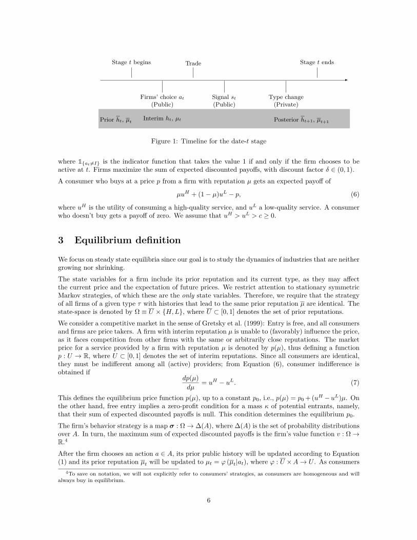
Figure 1: Timeline for the date-t stage

where 1at 6=I is the indicator function that takes the value 1 if and only if the firm chooses to beactive at t. Firms maximize the sum of expected discounted payoffs, with discount factor δ ∈ (0, 1).A consumer who buys at a price p from a firm with reputation µ gets an expected payoff of

µuH + (1− µ)uL − p, (6)

where uH is the utility of consuming a high-quality service, and uL a low-quality service. A consumerwho doesn’t buy gets a payoff of zero. We assume that uH > uL > c ≥ 0.

3 Equilibrium definition

We focus on steady state equilibria since our goal is to study the dynamics of industries that are neithergrowing nor shrinking.The state variables for a firm include its prior reputation and its current type, as they may affectthe current price and the expectation of future prices. We restrict attention to stationary symmetricMarkov strategies, of which these are the only state variables. Therefore, we require that the strategyof all firms of a given type τ with histories that lead to the same prior reputation µ are identical. Thestate-space is denoted by Ω ≡ U × H,L, where U ⊂ [0, 1] denotes the set of prior reputations.We consider a competitive market in the sense of Gretsky et al. (1999): Entry is free, and all consumersand firms are price takers. A firm with interim reputation µ is unable to (favorably) influence the price,as it faces competition from other firms with the same or arbitrarily close reputations. The marketprice for a service provided by a firm with reputation µ is denoted by p(µ), thus defining a functionp : U → R, where U ⊂ [0, 1] denotes the set of interim reputations. Since all consumers are identical,they must be indifferent among all (active) providers; from Equation (6), consumer indifference isobtained if

dp(µ)dµ

= uH − uL. (7)

This defines the equilibrium price function p(µ), up to a constant p0, i.e., p(µ) = p0 + (uH −uL)µ. Onthe other hand, free entry implies a zero-profit condition for a mass κ of potential entrants, namely,that their sum of expected discounted payoffs is null. This condition determines the equilibrium p0.The firm’s behavior strategy is a map σ : Ω→ ∆(A), where ∆(A) is the set of probability distributionsover A. In turn, the maximum sum of expected discounted payoffs is the firm’s value function v : Ω→R.4

After the firm chooses an action a ∈ A, its prior public history will be updated according to Equation(1) and its prior reputation µt will be updated to µt = ϕ (µt|at), where ϕ : U ×A→ U . As consumers

4To save on notation, we will not explicitly refer to consumers’ strategies, as consumers are homogeneous and willalways buy in equilibrium.

6

do not distinguish among entrants with new names (i.e., those who chose at = N) they will have thesame interim reputation µE , which is also constant over time. Given an interim reputation µt and asignal realization st, the posterior probability that the firm is competent is denoted by ϕ (µt|st), whereϕ : U× ((0, 1) ∪ ∅)→ U . Under these beliefs, the maximization of expected, discounted lifetime profitsin recursive form is associated with the following Bellman equation:

v (µ, τ) = maxσ∈∆(A)

(σO + σN )(p0 − c) + (uH − uL)(σOϕ(µ|O) + σNϕ(µ|N))

+ δ∑

τ ′∈H,L

λττ′(∫ 1

0

[σOv (ϕ(ϕ(µ|O)|r), τ ′) + σNv(ϕ(ϕ(µ|N)|r), τ ′)

]dF τ

+ σIv(ϕ(ϕ(µ|I)|∅), τ ′))

, (8)

where σa denotes the probability that the firm chooses action a, with∑a σa = 1. The resulting policy

function is denoted by σa(µ, τ) ≡ Pr(a|µ, τ).While firms may have heterogeneous and ever-changing reputations, in the steady state the reputationdistribution is constant over time. G denotes the cdf of prior reputations of active firms at thebeginning of each stage; mτ denotes the mass of type-τ firms in that group. Similarly, G denotes thecdf of interim reputations of active firms, and mτ the corresponding mass of type-τ firms. Thus, Gand G differ because some incumbents choose to exit, some to re-enter, and some inactive firms decideto enter.In equilibrium firms maximize their discounted expected profits, the market clears, consumers’ expec-tations are correct and satisfy Bayes’ rule whenever possible, and the population distributions of firms’reputations are constant over time:

Definition 1 (Equilibria). An equilibrium is a strategy σ∗, a price function p, and a belief system(ϕ,ϕ) with corresponding distributions (G,G) such that:

i. Optimality: σ∗ : Ω→ ∆(A) is the policy function associated with Equation (8);ii. Market clearing: The mass of active firms equals the mass of consumers: mH +mL = 1;iii. Consistency of beliefs: Firms’ reputations are derived from σ∗ using Bayes’ rule wheneverpossible;iv. Steady state: The reputation distributions of active firms G and G and the entrants’ reputa-tion are constant over time.

As is common in this kind of models, many equilibria may exist, supported by different beliefs. Wefocus on the class of reputational name-switching equilibria in which the entrants’ reputation acts asa “reservation reputation”: firms with reputations above µE keep their names, while any firm whosereputation falls below µE switches its name.

Definition 2 (Name-switching equilibria). An equilibrium where firms use the following strategyσ∗(µ, τ) is called name-switching equilibrium:

(σ∗O(µ, τ) σ∗N (µ, τ) σ∗I (µ, τ)) ≡

(

0 1 0)

if µ < µE ∧ τ = H,(0 ξ 1− ξ

)if µ < µE ∧ τ = L,(

1 0 0)

if µ ≥ µE ∧ (τ = H ∨ τ = L),

(9)

for some ξ ∈ (0, 1) and for some µE ∈ [0, 1].

7

In this equilibrium class competent firms always produce, as do inept firms with prior reputation aboveµE . Active firms sell under their old names if and only if their prior reputations are above µE . Ineptfirms with prior reputation below µE are indifferent between being active or inactive; they produceunder a new name with probability ξ, and stay inactive with probability 1− ξ. Observe that if µE ishigher than λLH there will be entry and exit flows in equilibrium; if, on the other hand, µE is lowerthan λHH , a positive mass of firms will keep their names, giving thus rise to a non-trivial industrydynamics. The next section shows that this is indeed the case.

4 Equilibrium characterization

4.1 Belief updating

Bayesian updating conditioning on a and µ yields

ϕ(µ|a) = σa (µ,H)µσa (µ,H)µ+ σa (µ,L) (1− µ) (10)

whenever σa(µ, τ) > 0 for some τ ∈ H,L. When µ ≥ µE , both types are expected to keep theirnames (a = O) so that the action is uninformative. On the other hand, a = O is a zero-probabilityevent when µ < µE ; in this case, we assume that such off-equilibrium move is also uninformative:

ϕ(µ|O) = µ ∀µ ∈ U (11)

When a ∈ N, I, h becomes unobservable, so that conditioning on µ is not possible. In this case,consistency of beliefs requires that the interim reputation for firms choosing each action be equal tothe fraction of competent firms in that group (if non-empty), given σ∗. Thus, the entrants’ reputationϕ(µ|N) satisfies

µE = mHG (µE |H) + λLHκ

G (µE)(12)

whenever G(µE) > 0. In fact, in the steady state the mass of entrants (i.e., new names) is equal to themass of firms that exit (i.e., the mass of lost names G(µE)); the competent “entrants”, in turn, arethe inactive firms that become competent (with mass λLHκ) plus the competents that exited in orderto change their names (with mass mHG(µE |H)). Similarly, the interim reputation of inactive firmsϕ(µ|I) is null as no competent chooses this action.Hence, there are two cases in which the interim reputation would differ from the prior: either the namechanged, or the action is perfectly revealing.Summarizing, the interim reputation is given by

ϕ(µ|a) =

µ if a = O,

µE if a = N ,0 if a = I.

(13)

After a signal r ∈ (0, 1) is realized, the interim reputation of an active firm is updated to

ϕ (µ|r) = λLH + (λHH − λLH) fH (r)µfH (r)µ+ fL (r) (1− µ) , (14)

which amounts to Bayes’ rule upon consideration of the possibility of type-change. Since fH andfL have full support, Equation (14) is well-defined for all µ ∈ [0, 1] and r ∈ (0, 1). Notice that the

8

assumption that (λHH − λLH) > 0 implies that the posterior reputation is strictly increasing in theinterim reputation.Regarding inactive firms, Bayes’ rule requires their posterior reputation to be

ϕ (µ|∅) = λLH (15)

as they are subject to the same type change process.

As the likelihood ratio fH(r)fL(r) is a monotonically increasing bijection from (0, 1) to (0,∞), it follows

that the range of prior reputations is U = [λLH , λHH ], and the range of interim reputations is U =[λLH , λHH ] ∪ 0, µE.Consistency of beliefs requires also that the mean prior and the mean interim reputation of activefirms are mH and mH respectively. Moreover, for any x ∈ U , the probability of being competentconditional on the firm’s prior reputation being x is exactly x. If the reputation distributions areabsolutely continuous, this translates into

mHg (x|H)g (x) = x, (16)

where g (·|τ) denotes the pdf of prior reputations conditional on current type τ , and g (·) denotes theunconditional pdf.

4.2 Optimality and market clearing in steady state

We now turn to requirements i and ii. Given the equilibrium beliefs, the value function in Equation(8) is given by

v (µ, τ) = maxσ∈∆(A)

(σO + σN )(p0 − c) + (uH − uL)(σOµ+ σNµE)

+ δ∑

τ ′∈H,L

λττ′(∫ 1

0

[σOv (ϕ(µ|r), τ ′) + σNv(ϕ(µE |r), τ ′)

]dF τ + σIv(λLH , τ ′))

)(17)

for a firm of prior reputation µ and current type τ . The flow payoff (σO+σN )(p0−c)+(uH−uL)(σOµ+σNµE) and the law of motion ϕ are continuous and non-decreasing functions in µ. On the other hand,the signal for a competent firm first-order stochastically dominates that of an inept one. It followsthat the value function is non-decreasing in µ for both types, and that the value for the competenttype is larger than the value for an inept type at any reputation level.5

The fact that the value function is non-decreasing in µ implies that any firm with prior reputationbelow µE that chooses to produce will sell under a new name; hence, σ∗O(µ, τ) = 0 is indeed optimalif µ < µE .On the other hand, as v (µ,H) > v (µ,L), it follows that market clearing (Requirement ii) amounts toa zero-profit condition that is binding only for inept entrants, namely,

v (µE , L) = 0. (18)

As the flow payoff is linear in p0, for each cost level c ∈ R+ there will be one p0 ∈ R such that Equation(18) holds. As a consequence, the policy function in Equation (9) is indeed optimal (Requirement i).

5Let N be the set of bounded, continuous, non-decreasing functions that map R2 into R, endowed with the sup norm.Let us associate type τ = L to the number 0, and type τ = H to 1. Then, the Bellman operator maps N into N , and asN is a closed subset of the set of continuous and bounded functions, its unique fixed point v also lies in this set. (See,for instance, Theorem 1.6, Lemma 1.8 and Lemma 1.10 in Chapter 12 of De la Fuente (2000)).

9

The levels of mH and mL are determined by the firms’ strategies and the market clearing condition(Requirement ii), taking into account the type-change process. The type-change process applied toactive firms yields (

mH

mL

)=(λHH λLH

λHL λLL

)(mH

mL

). (19)

The same transition matrix Λ applies to inactive firms; hence, after the mass of λLHκ of inactive firmsthat become competent enters the market, with the corresponding exit of an equal mass of inept firms,we obtain (

mH

mL

)=(mH

mL

)+(

λLHκ−λLHκ

). (20)

Solving for mH and taking into account that mH +mL = 1, we obtain

mH = λLH

λLH + λHL(1 + κ). (21)

The upper bound on κ in Equation (4) implies that mH < λHH . As consistency of beliefs implies thatmH is the mean interim reputation, this assumption rules out the case in which all firms change theirnames at all times.After all inept firms with µ < µE leave the market, the mass of inept potential entrants ismLG (µE |L)+λLLκ. Since the mass of inept firms with µ > µE is mL

(1−G (µE |L)

), then the equilibrium behavior

strategy ξ for inept firms under the threshold µE must satisfy

ξ(mLG (µE |L) + λLLκ

)+mL

(1−G (µE |L)

)= mL.

Rearranging and using Equation (20), we get

ξ = mLG (µE |L)− λLHκmLG (µE |L) + λLLκ

. (22)

4.3 Distributions and entrants’ reputation in steady state

Let r (x, µ) denote the signal that a firm with interim reputation µ needs to obtain a posterior repu-tation x, and µ (x, r) denote the interim reputation that a firm requires to get a posterior reputationx after a signal r. Both functions are defined implicitly by

x =ϕ(µ|r(x, µ)) and (23)x =ϕ(µ(x, r)|r), (24)

where ϕ is defined by Equation (14). Let γττ ′ ≡ mτ

mτ ′ λττ′ denote the fraction of type-τ ′ firms at

the beginning of any particular period that were type-τ in the previous period. We know that∑τ∈H,L γ

ττ′ = 1 and γHH > γHL. The prior reputation distribution for current type-τ ′ firms isa mixture of the posterior reputation distributions for previously type-H and type-L firms, where γHτ′

and γLτ′ are the corresponding mixture weights. Thus, the steady-state conditional distributions of

prior and interim reputations for active firms satisfy(G (x|H)G (x|L)

)=(γHH γLH

γHL γLL

)( ∫ r(x,µE)0 G (µ (x, r) |H) dFH∫ r(x,µE)0 G (µ (x, r) |L) dFL

). (25)

Equation (25) shows the prior reputation distributions of competent and inept active firms, respectively,as a function of the previous period’s interim reputation distributions. From each particular group of

10

firms, the firms with reputation smaller than or equal to x are those that in the previous period hadan interim reputation no greater than µ (x, r) whose signal realization was r; the measure of the groupthat originally was type-τ is

∫ r(x,µE)0 G (µ (x, r) |τ) dF τ . The integrals go from 0 to r (x, µE) because

a signal higher than r (x, µE) is required to reach a reputation x today only if the interim reputationwas smaller than µE .In turn, the distributions of interim reputations conditional on type τ are given by

G (x|τ) =

0 if x < µE ,1mτ

((mτ −mτ ) +mτG (x|τ)

)if x ≥ µE .

(26)

The interim distributions in Equation (26) take into consideration the strategy σ∗, and hence differfrom the prior distributions in two respects: (1) the entry of a mass λLHκ of inactive firms that becomecompetent, which replaces an equal mass of inept firms; and (2) the changing of names by firms withpriors lower than µE that remain active.The next theorem establishes that there is a unique consistent tuple of steady-state conditional distri-butions for active firms and entry-level reputation:

Theorem 1. There is a unique tuple(µE , G (·|H) , G (·|L)

)of entry-level reputation and steady-state

reputation distributions for active firms that jointly satisfy equations (25) and (26), and such that µEsatisfies Equation (12). The reputation distributions are absolutely continuous, with support [λLH , λHH ]for the prior reputation distributions G (·|τ) and [µE , λHH ] for the interim reputation distributionsG (·|τ), and µE ∈

(λLH ,mH

).

Theorem 1 asserts that the steady-state reputation distributions and the entry-level reputation areuniquely determined. Uniqueness is not only computationally useful but economically significant, asit implies that the level of p0 that solves the free-entry condition in Equation (18) is also uniquelydetermined. Therefore, the equilibrium is unique in its class.A sketch of the proof is as follows: First, think of µE as a parameter. Replacing Equation (26)in Equation (25), we see that the pair of prior distributions

(G (·|H) , G (·|L)

)is the fixed point of

an operator. Theorem 1 establishes the existence and uniqueness of this fixed point which dependscontinuously on µE , and also on the parameters of the transition matrix Λ and on κ. The limitingdistributions are absolutely continuous; hence, Equation (16) applies.Now, consider a fixed pair of reputation distributions for competent and inept firms. The fraction ofcompetent firms among entrants is given by the right-hand side of Equation (12), which we define asthe function ψ : (λLH , λHH ]→ [0,∞):

ψ (x) ≡ mHG (x|H) + λLHκ

G (x). (27)

Thus, Equation (12) says that any consistent entry-level reputation µE is a fixed point of the functionψ defined by Equation (27). Such a fixed point exists: The sets x : x < ψ (x) and x : x > ψ (x)are non-empty and ψ is continuous.6 On the other hand, observe that for any given cutoff value x,ψ (x) is the average reputation among entrants while x is the reputation of the marginal entrants.Then, the average reputation is increasing (resp., decreasing) if and only if the marginal reputation isabove (resp., below) it. It follows that ψ′ = 0 if and only if x = ψ (x) and therefore the fixed point isunique: There is a unique value of µE at which the cutoff point coincides with the expected fractionof competents in the group of entrants. This is illustrated with a numerical example in Figure 2.

6In fact, the function ψ (x) is constructed under the assumption that firms change their names if and only iftheir reputation falls below the cutoff x and all competents enter. Consider the value x∗ ∈ (λLH , λHH) that satisfiesmLG (x∗|L) = λLHκ; in that case, all entrants are competent and their reputation is the highest possible: ψ (x∗) = 1,and therefore x∗ ∈ x : x < ψ (x). On the other hand, at x = λHH all firms exit and ψ (x) = mH < λHH , so thatx : x > ψ (x) is also non-empty.

11

0 0.2 0.4 0.6 0.8 10

0.1

0.2

0.3

0.4

0.5

0.6

0.7

0.8

0.9

1

µ

ψ(µ)

Figure 2: Consistent entry-level reputation as a fixed pointNotes: fH (r) = Be (r|3, 2) and fL (r) = Be (r|2, 3). The parameters are λHL = 0.075, λLH =0.025 and κ = 1. The resulting µE is 0.26.

Notice that µE must be strictly larger than λLH , so that a positive mass of firms chooses to becomeinactive, making room for the entrants. At the same time, the mean interim reputation for active firmsmust be larger than µE , the minimum reputation in the support of the distribution; as consistency ofbeliefs implies that this mean reputation is mH , we conclude that µE ∈ (λLH ,mH).

Moreover, Equation (16) implies that g(x|H)g(x|L) is increasing in x and thus the ratio g(x|H)

g(x|L) is also increas-ing. In other words, consistency of beliefs implies that the monotone likelihood ratio property–whichis assumed for the distributions of signals conditional on types–extends to the distributions of repu-tations conditional on types in the population of active firms. As likelihood ratio dominance impliesfirst-order stochastic dominance, it follows that:

Corollary 1 (Reputation across types). The distribution of reputations (both prior and interim) ofcompetent firms first-order stochastically dominates that of inept firms. Formally, (∀x ∈ [λLH , λHH ]),

G (x|H) ≤ G (x|L) and G (x|H) ≤ G (x|L)

with strict inequality in the interior.

The proof of Theorem (1) goes beyond our previous discussion, in that it considers simultaneouslythe consistency of the entry-level reputation µE and the distributions (G (·|H) , G (·|L)). Clearly,µE affects the shape of the steady-state distributions: No firm would ever keep its name should itsreputation fall below that threshold, and the interim distributions would have a point mass at µEevery period (namely, the mass of firms that enter).

5 Comparative statics

The parameter λLH , the probability for an inept firm to become competent, measures the rate at whichcompetency is acquired–a sort of technical progress or product innovation. In our model, this rate isexogenous and homogeneous among firms; Section 7 below contains a brief discussion of endogeneityand heterogeneity. The parameter λHL, on the other hand, measures the depreciation rate of this skill.We are interested in how the rates of competency acquisition λLH and depreciation λHL, and out-side competitive pressure κ shape the equilibrium. Not only the steady-state distributions depend

12

continuously on them; the entry-level reputation does as well, as Proposition 1 asserts:

Proposition 1 (Continuous dependence on parameters). The tuple (µE , G (·|H) , G (·|L)) of entry-level reputation and steady-state reputation distributions depends continuously on the parameters ofthe transition matrix Λ and on κ.

As an immediate corollary, the exit rate G(µE) is also continuous on those parameters.The level of the entrants’ reputation is affected by κ and the transition parameters λHL and λLH ina non-trivial way, as they affect mτ and mτ differently. In particular, the effects of changes in λHL

and λLH over µE are not symmetric: While λHL only affects the transition matrix in Equation (19),λLH also affects the entry flow of new competent firms in Equation (20). What is symmetric, however,is that any change in parameters that results in higher values of γHL and γLH without reducing λLHκimplies a higher µE :

Proposition 2 (Comparative statics). The entry-level reputation µE increases after any change inthe parameters of the transition matrix Λ or κ that results in a increase in the mixture weights γHLand γLH without reducing the entry flow of new competent firms λLHκ.

Increasing γHL and γLH means that the gap between γHH and γHL shortens; therefore, the prior repu-tation distributions for competent and inept firms move closer to each other. By this mechanism, theadverse selection that entrants face is reduced, as the fraction of competent firms among those belowthe threshold increases. Hence, provided that λLHκ is not reduced, an increase in γHL and γLH causesµE to increase.Consider first an increase in λHL, which affects only active firms in equilibrium. Intuitively, a higherλHL implies a higher “depreciation rate” of information, as the weight of older signals in predictingthe current firm type decreases. Histories become less informative about types and the mixing weightsγHL and γLH are increased; hence, the composition of the pool of firms changing their names improves.Therefore, the effect of an increase in λHL over µE is unambiguous: the entrants’ reputation increasesafter an increase in λHL. The same result obtains if the increase in λHL is compensated, either by aproportional increase in λLH or by an increase in κ, so that mH remains fixed.The case of an isolated increase in λLH is different, however, because this type-change probability notonly affects active firms but also inactive ones. A higher λLH implies a higher mH as active inept firmsare more likely to become competent; the effect over mH is proportionally larger, however, becausea higher flow of new competent firms is added to mH at each period. This implies that the mixingweight γLH decreases after an increase in λLH , so that the sufficient condition in Proposition 2 is notmet.Finally, µE increases if λHL and λLH jointly increase while κ decreases so that the flow of new competentfirms λLHκ does not change, and both mH and mH remain constant. Figure 3 illustrates this case.Proposition 3 below summarizes these results:

Proposition 3. The sufficient conditions for an increase in µE from Proposition 2 are met in all thefollowing circumstances:

1. An increase in λHL;

2. A proportional increase in λHL and λLH;

3. An increase in λHL and κ so that mH remains constant;

4. An increase in λHL and λLH, and a reduction in κ such that mH and mH remain constant.

13

0 0.2 0.4 0.6 0.8 10

0.1

0.2

0.3

0.4

0.5

0.6

0.7

0.8

0.9

1

µ

G(µ|τ)

G(µ|H)

G(µ|L)

(a) Distributions G(µ|H) and G(µ|L)

0 0.2 0.4 0.6 0.8 10

0.1

0.2

0.3

0.4

0.5

0.6

0.7

0.8

0.9

1

µ

ψ(µ)

(b) Fraction of competents among entrants ψ(µ)

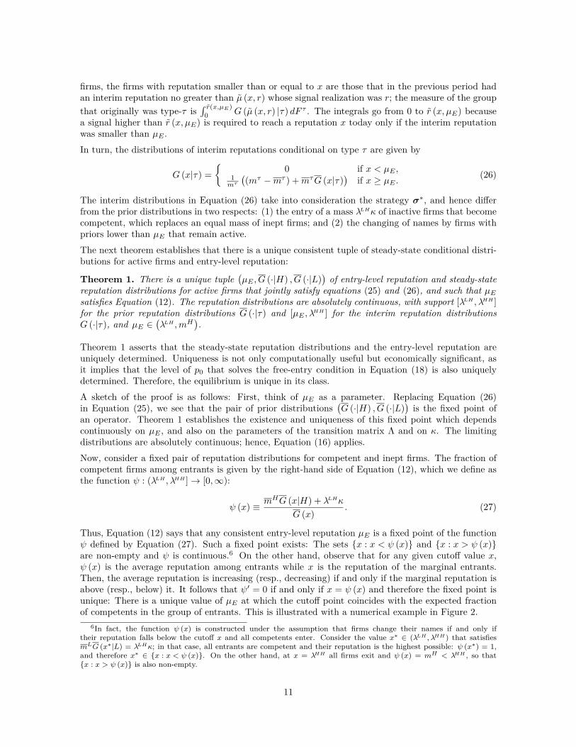
Figure 3: Distributions and entry-level reputation for different combinations of λLH , λHL and κ.Notes: fH (r) = Be (r|3, 2) and fL (r) = Be (r|2, 3). The parameters are λHL = 0.075, λLH = 0.025 and κ =1 (solid line) and λHL = 0.275, λLH = 0.225 and κ = 1/9 (dotted line), so that mH = 0.5 and mH = 0.475in both cases. The resulting µE is 0.26 in the first case and 0.43 in the second one.

6 Industry dynamics

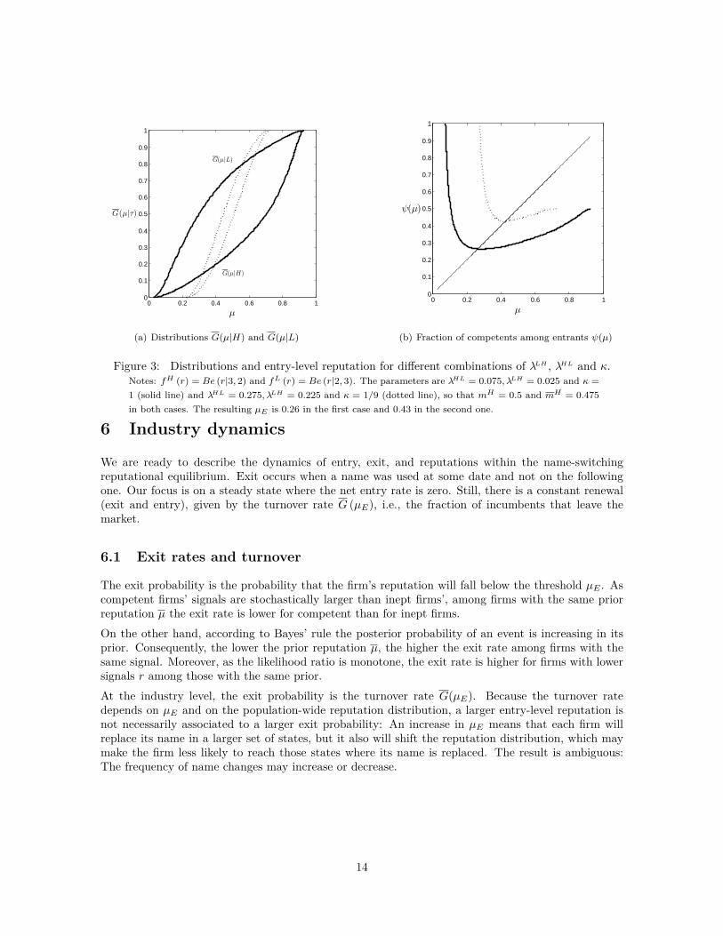
We are ready to describe the dynamics of entry, exit, and reputations within the name-switchingreputational equilibrium. Exit occurs when a name was used at some date and not on the followingone. Our focus is on a steady state where the net entry rate is zero. Still, there is a constant renewal(exit and entry), given by the turnover rate G (µE), i.e., the fraction of incumbents that leave themarket.

6.1 Exit rates and turnover

The exit probability is the probability that the firm’s reputation will fall below the threshold µE . Ascompetent firms’ signals are stochastically larger than inept firms’, among firms with the same priorreputation µ the exit rate is lower for competent than for inept firms.On the other hand, according to Bayes’ rule the posterior probability of an event is increasing in itsprior. Consequently, the lower the prior reputation µ, the higher the exit rate among firms with thesame signal. Moreover, as the likelihood ratio is monotone, the exit rate is higher for firms with lowersignals r among those with the same prior.At the industry level, the exit probability is the turnover rate G(µE). Because the turnover ratedepends on µE and on the population-wide reputation distribution, a larger entry-level reputation isnot necessarily associated to a larger exit probability: An increase in µE means that each firm willreplace its name in a larger set of states, but it also will shift the reputation distribution, which maymake the firm less likely to reach those states where its name is replaced. The result is ambiguous:The frequency of name changes may increase or decrease.

14

6.2 Age

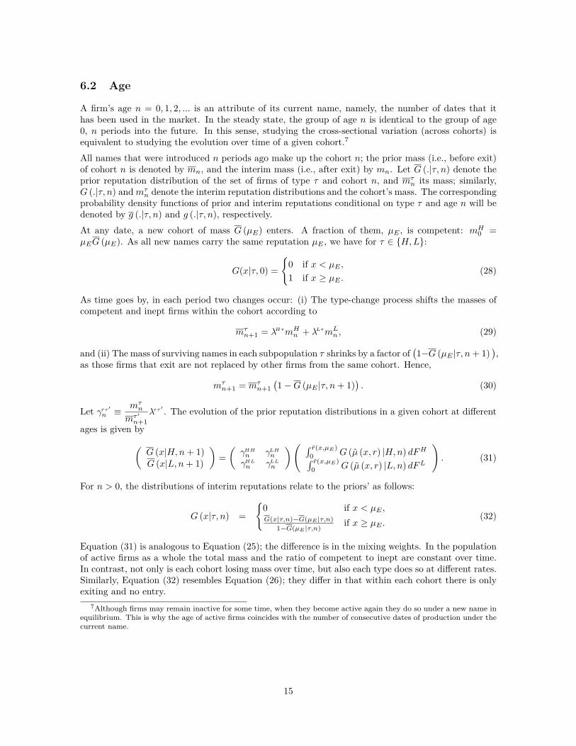
A firm’s age n = 0, 1, 2, ... is an attribute of its current name, namely, the number of dates that ithas been used in the market. In the steady state, the group of age n is identical to the group of age0, n periods into the future. In this sense, studying the cross-sectional variation (across cohorts) isequivalent to studying the evolution over time of a given cohort.7

All names that were introduced n periods ago make up the cohort n; the prior mass (i.e., before exit)of cohort n is denoted by mn, and the interim mass (i.e., after exit) by mn. Let G (.|τ, n) denote theprior reputation distribution of the set of firms of type τ and cohort n, and mτ

n its mass; similarly,G (.|τ, n) andmτ

n denote the interim reputation distributions and the cohort’s mass. The correspondingprobability density functions of prior and interim reputations conditional on type τ and age n will bedenoted by g (.|τ, n) and g (.|τ, n), respectively.At any date, a new cohort of mass G (µE) enters. A fraction of them, µE , is competent: mH

0 =µEG (µE). As all new names carry the same reputation µE , we have for τ ∈ H,L:

G(x|τ, 0) =

0 if x < µE ,

1 if x ≥ µE .(28)

As time goes by, in each period two changes occur: (i) The type-change process shifts the masses ofcompetent and inept firms within the cohort according to

mτn+1 = λHτmH

n + λLτmLn , (29)

and (ii) The mass of surviving names in each subpopulation τ shrinks by a factor of(1−G (µE |τ, n+ 1)

),

as those firms that exit are not replaced by other firms from the same cohort. Hence,

mτn+1 = mτ

n+1(1−G (µE |τ, n+ 1)

). (30)

Let γττ′n ≡

mτn

mτ ′n+1

λττ′ . The evolution of the prior reputation distributions in a given cohort at different

ages is given by(G (x|H,n+ 1)G (x|L, n+ 1)

)=(γHHn γLHnγHLn γLLn

)( ∫ r(x,µE)0 G (µ (x, r) |H,n) dFH∫ r(x,µE)0 G (µ (x, r) |L, n) dFL

). (31)

For n > 0, the distributions of interim reputations relate to the priors’ as follows:

G (x|τ, n) =

0 if x < µE ,G(x|τ,n)−G(µE |τ,n)

1−G(µE |τ,n)if x ≥ µE .

(32)

Equation (31) is analogous to Equation (25); the difference is in the mixing weights. In the populationof active firms as a whole the total mass and the ratio of competent to inept are constant over time.In contrast, not only is each cohort losing mass over time, but also each type does so at different rates.Similarly, Equation (32) resembles Equation (26); they differ in that within each cohort there is onlyexiting and no entry.

7Although firms may remain inactive for some time, when they become active again they do so under a new name inequilibrium. This is why the age of active firms coincides with the number of consecutive dates of production under thecurrent name.

15

6.2.1 Differences across types

Starting from the interim reputation distribution for new firms in Equation (28) and applying equations(31) and (32), it can be shown by induction that for all n ∈ N,

mHn g (x|H,n)mng (x|n) = x. (33)

Equation (33) is the analogous to Equation (16) when conditioning on age. Consistency of beliefs thusimplies the monotone likelihood ratio property of the distributions of reputations conditional on typeswithin cohorts, as the likelihood ratios g(x|H,n)

g(x|L,n) and g(x|H,n)g(x|L,n) are increasing in x. It follows that:

Proposition 4 (Reputation across types by cohort). Within each cohort n ≥ 1 the (prior, interim)reputation of competent firms first-order stochastically dominates the (prior, interim) reputation ofinept firms. Formally, (∀n ∈ N) (∀x ∈ [λLH , λHH ]),

G (x|H,n) ≤ G (x|L, n) and G (x|H,n) ≤ G (x|L, n) ,

with strict inequality in the interior.

In view of the linear connection between prices and interim reputations and the connection betweenexit rates and prior distributions, Proposition 4 implies:

Corollary 2. Competent firms charge higher prices (in a stochastic sense) and exit less often thaninept firms, both within each cohort and throughout the population.

6.2.2 Differences across cohorts

Clearly, the interim reputation of older cohorts first-order stochastically dominates that of the cohortof age 0. As the equilibrium price is a linear function of the firms’ interim reputation, the pricedistributions inherit the properties of the interim reputation distributions. In particular, the pricethat older cohorts charge first-order stochastically dominates that of entrants.On the other hand, the exit (or name-switching) decision is made in response to the prior reputation.The next proposition shows that the prior reputation of older cohorts also first-order stochasticallydominates that of age 1, which implies that the exit probability of older firms is smaller.

Proposition 5 (Reputation across cohorts). The prior reputation of firms of age 1 is first-orderstochastically dominated by the prior reputation of firms of any older cohort, both conditional andunconditional on types. Formally, (∀n ∈ N) (∀x ∈ [λLH , λHH ]):

G (x|τ, n) ≤ G (x|τ, 1) and G (x|n) ≤ G (x|1) ,

with strict inequality in the interior for n > 1.

Again, the connection between the prior distribution and the exit rate implies:

Corollary 3. Older firms exit less often than firms of age 1, both conditioning and not conditioningon type.

Figure 4 shows the family of prior reputation distributions by cohorts in a numerical example whereolder firms (i.e., names) have stochastically better reputations than younger ones. This means that exitrates are monotonically decreasing in age, and the price distributions are also ordered by first-orderstochastic dominance.

16

0 0.2 0.4 0.6 0.8 10

0.1

0.2

0.3

0.4

0.5

0.6

0.7

0.8

0.9

1

µ

n= 1

n= 2

n= 3

n= 4

n= 5

n= 6, 7, 8...

µE

G(µ|n)

Figure 4: Reputation distributions for different ages, G (µ|n)Notes: fH (r) = Be (r|3, 2) and fL (r) = Be (r|2, 3). The parameters are λHL = 0.075, λLH =0.025 and κ = 1. The resulting µE is 0.26.

6.3 Relation to empirical literature

The empirical literature on industry dynamics finds considerable heterogeneity among industries interms of entry and exit rates. Typically, gross entry and exit rates are similar within an industry(Dunne et al., 1988). The focus on the steady state is thus particularly suitable for analyzing thoseindustries.The analysis in Section 6.1 suggests that heterogeneity among firms within an industry should alsobe expected: The exit probability is higher for names with worse reputations and/or worse signals.The empirical literature is consistent with these predictions: Cabral and Hortacsu (2010), in a studyof eBay auctions, find that the probability that a name exits the market increases as its reputationdeclines (as defined by eBay’s reputation mechanism.) In turn, McDevitt (2011) studies the plumbingservices market in Illinois and finds that, all else being equal, the firms more likely to change namesor withdraw are those with worse track records–a variable that resembles the history of public signalsin our model.The analysis also shows that inept firms are more likely to leave the market than competent ones.Although types are unobservable to the econometrician, this proposition has testable implications: Asthe exit process is biased towards inept firms, older firms have (stochastically) larger reputations thanyounger firms, as Proposition 5 asserts. Moreover, since firms with better reputations charge higherprices, this implies that older firms charge (stochastically) larger prices. These predictions are alsoconsistent with the empirical literature, which finds systematic differences between firms of differentages: In Foster et al. (2008) younger firms are more likely to exit, and charge lower prices, than olderfirms. In the same vein, in McDevitt (2011) the exit probability is monotonically decreasing with age.Moreover, while these studies find a strong positive relation between survival and age, quality mayexplain the apparent correlation between those variables (Thompson, 2005).In view of these findings, one would expect a selected sample of old, highly reputable firms to changenames at a low rate; this is precisely what Wu (2010) finds when examining CRSP-listed companies.Correspondingly, an unbiased sample of firms within an industry should exhibit a (perhaps consider-ably) higher incidence of name-switching, just as McDevitt (2011) finds in the Illinois plumbing-serviceindustry.The previous discussion suggests that a reputation-based model can be very helpful in improving our

17

understanding of industry dynamics.

7 Discussion

The model developed in this paper is almost as simple as possible within the class of dynamic adverseselection models: There are two types, all long-run players use the same behavior strategy σ∗–whichdepends on the simplest state space–, and the attention is centered on the steady state. Imperfectpublic monitoring coupled with a type-change process results in a market with a continuum of firmswith different reputations charging different prices. Reputation heterogeneity is limited by strategicexit and entry: Firms have the option to reset their reputations by exiting the market and reenteringunder a new name.Many features of the model may be amended without essential effects on the equilibrium dynamics:Moral hazard. Probably the foremost real-world issue that was left aside is moral hazard. However,the dynamics studied here under the assumption that competent firms can only provide high qualityare the same as those of a model where competent firms choose to do so. The conditions under whichthey do are studied in Vial and Zurita (2013) in a similar setting.Long-lived consumers. In many real-world examples–some of which the cited literature describes–consumers purchase more than once. If long-lived consumers accumulate private information based ontheir experiences with suppliers, the belief homogeneity exploited in this paper breaks down, openingup the possibility of relationship-building. What is crucial to the results in a setting with a continuumof buyers and sellers, however, is the type of monitoring rather than the repeated interaction betweenthem. For instance, in Mailath and Samuelson (2001) consumers are long-lived, but monitoring remainspublic.8 Thus, our model can be interpreted as one with long-lived consumers and public monitoringas well.Type change vs. replacement. The effect of the type change process in our model is to permanently“replenish” the uncertainty about types, i.e., to put tighter upper and lower bounds on reputations.We could instead consider an exogenous replacement process with the same effect.9 By the replacementprocess, any name can pass from an old firm to a new one. Let’s define λ and θ so that λLH = λθ andλHL = λ (1− θ), while λLH + λHL = λ. Then λ could be interpreted as the probability that an activefirm is replaced (i.e., dies); if this event occurs, the name of the old firm is (randomly) assigned to anew competent firm with probability θ ∈ (0, 1) and to a new inept firm with probability 1− θ. As theconsequence of replacements and type-changes are identical from the consumer’s point of view, theinterim reputation would still be updated according to Bayes’ rule in Equation (14). So, if the prioris updated according to Equation (13), the value function for a firm of prior reputation µ and type τwould instead be given by

v (µ, τ) = maxσ∈∆(A)

(σO + σN )(p0 − c) + (uH − uL)(σOµ+ σNµE)

+ δ(1− λ)(∫ 1

0

[σOv (ϕ(µ|r), τ) + σNv(ϕ(µE |r), τ)

]dF τ + σIv(λLH , τ))

).

The policy functions, however, would not be affected: The strategy in Equation (9) is still optimal given8They assume that the ex post utility is the signal itself. If so, uτ would be the expected value of the signal conditional

on the quality that a type-τ seller provides, i.e., uH =∫ 1

0 rdFH and uL =∫ 1

0 rdFL. The condition uH > uL wouldfollow from stochastic dominance.

9We consider exogenous replacements. In contrast, Tadelis (1999) and Mailath and Samuelson (2001) study thepossibility of trading names when this trading is unobservable to consumers, while Wang (2011) and Hakenes and Peitz(2007) look at the observable trading case. Board and Meyer-ter Vehn (2013) and Dilmé (2012) consider the possibilityof choosing types.

18

consumers’ beliefs if p0 is such that v (µE , L) = 0. Moreover, as reputations and age are associated witha name and not with the identity of the firms that carry that name at different stages, the industrydynamics would not be affected. The only element of the name-switching equilibrium that would beaffected is the price function: The (unique) level of p0 that solves the free-entry condition v (µE , L) = 0would be lower under the type-changing process than under the replacement process, as firms have theoption to continue operating after a type change.Quality cost differentials. In our model, competent firms unambiguously profit more than ineptfirms of the same reputation. This follows from the monotone likelihood ratio property and theassumption that competent and inept firms have the same production cost. This assumption ensuresthat competent firms strictly prefer to enter when inept firms are merely indifferent, resulting in apool of entrants that is better than the pool of exiting firms. Instead, we could assume that competentfirms have higher costs than inept ones, as long as the advantage of having an easier road to higherreputations that the monotone likelihood ratio property entails outweighs the cost differential.The model showed the importance of the entry-level reputation as an equilibrating variable of themarket. This message is likely to extend to other environments. Further interesting extensions include:Differences between active and inactive firms. In our model, both active and inactive firmsare subject to the same type-change process. Let λLHa denote the type-change probability induced byaction a. There may be examples where the probability of becoming competent is different betweenactive and inactive firms: λLHO,N 6= λLHI . An interesting case occurs when the competency-acquisitionrate is positive only among active firms: λLHO,N > 0 and λLHI = 0. In that case, the adverse selectionproblem that entrants face is so acute that there are neither entry nor exit flows in equilibrium. Thisis due to the fact that the only competent entrants would be firms with bad histories that decidedto discard their names because their prior reputation was lower than µE , but consistency requiresthat the entrants’ reputation be the mean prior reputation in that group–a contradiction. Then, thegroup of entrants must be empty. In other words, names with a poor reputation are replaced by newnames if and only if λLHI > 0, as firms with poor reputation gain from pooling as new entrants withnew competents. Although two industries with the same mH would not differ in terms of the meanreputation of trading firms, their exit and entry flows would be completely different if λLHI > 0 in thefirst industry and λLHI = 0 in the second one.Endogenous types. A natural extension is giving firms the possibility of investing, or paying acost, to become competent prior to entry, as in Atkeson et al. (2015). The fact that competent firmshave an advantage over inept firms would generate a willingness-to-pay for an increased probabilityof becoming competent. The (endogenized) λLHI should adjust until the marginal firm is indifferentbetween investing or not. The adjustment would occur through the influence of λLHI on the entry-levelreputation and its effect on the payoff advantage of competent firms. Therefore, given equal productioncosts for both types of firms, λLHI > 0 would be an equilibrium outcome instead of an assumption.Furthermore, the type-change process may be endogenized by also enabling incumbent firms to invest,as in Board and Meyer-ter Vehn (2013): Firms may pay a cost to increase the probability of becomingcompetent in the next stage, λLHO,N . If most of the information that fosters innovative activity comes fromoutside the market, new firms would have an advantage over incumbent firms in acquiring competence;in contrast, if the main source of this information is nontransferable experience in the market, theadvantage would reverse.10

Entry or name-switching costs. Another interesting extension would be to consider an entrycost. If it were a sunk cost, it would create a wedge between the entry-level and exit-level reputations,as the value of entering would be smaller than the value of staying in the market, all else being equal.This would affect the turnover rate and the age distribution of firms, as the incentive for switchingnames would be reduced. The equilibrium price level would depend on the magnitude of the entrycost, as the free entry condition is binding for inept firms paying this cost. With moral hazard, this

10See Chapter 3 in Audretsch (1995).

19

would also have implications for efficiency, as discussed by Atkeson et al. (2015) and Garcia-Fontesand Hopenhayn (2000). A similar wedge would emerge if erasing the history (by changing names inour model) were costly (or risky); moreover, as the entry-level reputation is larger than the exit-levelreputation all entrants choose a new name in equilibrium. Thus, an entry cost is equivalent to aname-switching cost.

8 Conclusions

We presented a reputation model where industry dynamics is driven by the stochastic movement offirms’ reputations along with an option to change names. The constant renewal of names of disgracedfirms is prevalent in markets where identities can be changed or concealed at low cost; for instance, weobserve this with some Internet trading sites offering services such as home repair and maintenanceand with brick-and-mortar industries such as restaurants. Through a simple name-switching policy themodel rationalizes important features present in the data, like the positive correlation of reputationand price with age, and the negative correlation of reputation with exit.Beyond matching empirical findings, the model yields insight into the role of the different forces shapingthe equilibrium within a complex causality network. The preference parameters (consumers’ valuationsand firms’ discount factor and production costs) directly affect players’ choices, and through them, theequilibrium assignment and price function. For a given strategy profile, the informational variables (thedistribution of signals conditional on types, the parameters of the type-change process and the outsidecompetitive pressure) determine consumer beliefs. Still, the type-change process and the outsidecompetitive pressure are not merely informational variables, as they determine the composition offirms in the population. Since the price function solves a zero-profit condition that is binding formarginal entrants, it depends on the informational variables: While the entrants’ reputation affectstheir flow payoff, the expectation of future payoffs that stem from their subsequent reputations affecttheir continuation payoffs.The entrants’ reputation emerges as a key equilibrium variable that determines the name-switchingrate and therefore, the whole industry dynamics. The effect of the parameters of the transition processand the outside competitive pressure over the entry-level reputation is shown to depend crucially onits effect over the fraction of firms of a given type that were of the same type in the previous period:The lower this fraction, the closer to each other are the distributions for competent and inept firmsand the better the composition of the pool of name-switching firms is. Hence, industry dynamics aredriven by the endogenous name-switching process, while this is in turn determined by the exogenoustype-change process.While the results are obtained under a variety of simplifying assumptions, they are likely to be robust tothe consideration of important phenomena like moral hazard or differences in competency acquisitionand depreciation rates between active and inactive firms. Still, the analysis points towards manyinteresting questions for future research.

Appendix

A.1 Proof of Theorem 1We proceed in two steps. First, the entry-level reputation is assumed to be an exogenous parameter y ∈ (0, λHH). Underthis assumption, Lemma 1 shows that there is a unique steady-state distribution pair for competent and inept firms.

Second, the entry-level reputation y is endogenized by requiring it to be consistent: y = µE . Indeed, consistency impliesthat the fraction of competent firms among active firms with a given reputation µ is precisely µ, and similarly, that thefraction of competent firms among entrants (if any) is precisely µE . Lemma 2 shows that there is at least one consistententry-level reputation µE , while Lemma 3 shows that this entry-level reputation is unique.

20

Consider the system of integral equations defined by(Gt+1 (x|H)Gt+1 (x|L)

)≡(γHH γLH

γHL γLL

)( ∫ r(x,y)0 Gt (µ (x, r) |H) dFH∫ r(x,y)0 Gt (µ (x, r) |L) dFL

)(34)

and

Gt (x|τ) =

0 if x < y,1mτ

((mτ −mτ ) +mτGt (x|τ)

)if x ≥ y. (35)

Replacing Equation (35) in Equation (34) and rearranging, we get:(Gt+1 (x|H)Gt+1 (x|L)

)= λLHκ

(λHH

mH−λ

LH

mH

λHL

mL−λ

LL

mL

)(FH (r (x, y))FL (r (x, y))

)+

(λHH λLH mL

mH

λHLmH

mLλLL

)( ∫ r(x,y)0 Gt (µ(x, r)|H) dFH∫ r(x,y)0 Gt (µ(x, r)|L) dFL

). (36)

Alternatively, the change of variables µ = µ (x, r) and r = r (x, µ) (as defined in equations (24) and (23)) inside theintegral in Equation (36) allows it to be written as:(

Gt+1 (x|H)Gt+1 (x|L)

)= λLHκ

(λHH

mH−λ

LH

mH

λHL

mL−λ

LL

mL

)(FH (r (x, y))FL (r (x, y))

)−

(λHH λLH mL

mH

λHLmH

mLλLL

)( ∫ 1yGt (µ|H) fH (r(x, µ)) ∂r(x,µ)

∂µdµ∫ 1

yGt (µ|L) fL (r(x, µ)) ∂r(x,µ)

∂µdµ

). (37)

Define the right-hand side of Equation (36) (or alternatively, that of Equation (37)) as an operator T in the set of pairsof continuous and normalized functions

(G (·|H) , G (·|L)

)endowed with the following metric:11

ρ((G (·|H) , G (·|L)

),(G′ (·|H) , G′ (·|L)

))= max

ρ∞(G (·|H) , G′ (·|H)

), ρ∞

(G (·|L) , G′ (·|L)

),

where:ρ∞(G (·|τ) , G′ (·|τ)

)= supx∈[λLH ,λHH ]

∣∣Gτ (x|τ)−G′ (x|τ)∣∣

for τ ∈ H,L . The supremum is taken over x ∈ [λLH , λHH ] since the domains of G and G′ are always contained in thisinterval.

Note that equations (34) and (35) coincide with (25) and (26), respectively, in the steady state. As a consequence, thesteady-state reputation distributions G (·|H) and G (·|L) described in equations (25) and (26) are a fixed point of T .Since T depends parametrically on y, so do G (·|H) and G (·|L).

We start by establishing that:

Lemma 1. The operator T has a unique fixed point.

Proof. Notice that there are no firms with reputation either below y or above λHH after entry-exit decisions are made, andthat:

1. µ (x, r (x, y)) = y; this is to say, the previous reputation of a firm that obtained a signal r (x, y) that changedits reputation from y to x was y;

2. µ (x, r) < y ⇔ r > r (x, y): Those firms with a reputation x today and had a reputation lower than y in theprevious period are those that obtained signals of at least r (x, y); and

3. µ (x, r) > λHH ⇔ r < r (x, λHH): Those firms that had a higher reputation than λHH in the previous periodand have a reputation x today are those with signals lower than r (x, λHH).

Using these facts, the distance between Gt+1 (·|τ) and G′t+1 (·|τ) can be shown to be bounded as follows:

ρ∞(Gt+1 (·|τ) , G′t+1 (·|τ)

)≤ β · ρ

((Gt (·|H) , Gt (·|L)

),(G′t (·|H) , G′t (·|L)

)),

11As r(λLH , y) = 0, r(λHH , y) = 1, µ(λLH , r) = 0 and µ(λHH , r) = 1, if the functions Gt (·|τ) for τ ∈ H,L arenormalized, then Gt+1 (·|τ) are also normalized; i.e. Gt+1 (λLH |τ) = 0 and Gt+1 (λHH |τ) = 1.

21

where β ∈ (0, 1) is defined by

β = max

sup

x∈[λLH ,λHH ]

(FH (r (x, y))− FH

(r(x, λHH

))),

supx∈[λLH ,λHH ]

(FL (r (x, y))− FL

(r(x, λHH

))).

It follows that

ρ

((Gt+1 (·|H) , Gt+1 (·|L)

),(G′t+1 (·|H) , G′t+1 (·|L)

))≤ βρ

((Gt (·|H) , Gt (·|L)

),(G′t (·|H) , G′t (·|L)

)),

i.e., T is a contraction mapping with modulus β.

On the other hand, the set of continuous, bounded real functions endowed with the sup norm is complete. Moreover,the subset of normalized functions is closed, 12 and thereby complete. Then, by Banach’s fixed point theorem, T has aunique fixed point, which is a pair of continuous and normalized functions.

If y is consistent, G (x|H) and G (x|L) are increasing functions because G (x|H) and G (x|L) are non-negative in thewhole domain, while r (x, y) is increasing in x. Thus, G (x|H) and G (x|L) are not only normalized and continuous, butalso increasing. In other words, they are distribution functions.

The prior reputation distributions G (·|τ) have support [λLH , λHH ] because the likelihood ratio is onto; consequently, theinterim reputation distributions G (·|τ) have support [µE , λHH ]. All reputation distributions are absolutely continuousbecause the signal distributions are. Hence, Equation (16) applies. The parameter y affects the operator T , and thereforeaffects both the contraction modulus and the limiting distributions. Moreover, the limiting distributions are continuousin y, as they are the fixed point of a contraction.13 Similarly, the limiting distributions also depend continuously on theparameters κ and λττ′ for τ, τ ′ ∈ H,L. We write T y and Gy (x|τ) or T y;α and Gy;α (x|τ) to emphasize the dependenceof the operator and its fixed point in the cutoff level y or in any other parameter α when necessary.

We now endogenize the entry-level reputation y. Consider the function ψ : (λLH , λHH ]→ [0,∞) defined in Equation (27).Any consistent entry-level reputation must be a fixed point of ψ (see Equation (12)). When taking into considerationthe dependence of the distributions on y, ψ should be written as

ψ (x, y) =mHG

y (x|H) + λLHκ

mHGy (x|H) +mLG

y (x|L). (38)

Define the functionφ (µ) ≡ ψ (µ, µ) (39)

for µ ∈ (λLH , λHH ]. A consistent entry-level reputation satisfies µE = ψ (µE , y) for given distributions; now we need toverify that those distributions were generated by the same entry-level reputation: y = µE . In other words, we need toprove that φ (µ) has a unique fixed point. We begin by observing that:

Lemma 2. φ has at least one fixed point.

Proof. The function f (µ) ≡ Gµ (µ|L) is continuous, with f (λLH) = 0 and f (λHH) = 1. Then, by the Intermediate

Value Theorem there is at least one x∗ ∈ (λLH , λHH) such that f (x∗) = λLHκmL

, and so φ (x∗) = 1. We also know that φis continuous in its domain, and that φ (x∗)−x∗ = 1−x∗ > 0 and φ (λHH)−λHH = mH −λHH < 0 (as κ < κ as definedin Equation (4)). Also by the Intermediate Value Theorem, there is at least one µ ∈ (x∗, λHH) such that φ (µ)− µ = 0.As a consequence, there is at least one µE ∈ (λLH , λHH) such that ψ (µE , µE) = µE .

The next step is to establish uniqueness.

Lemma 3. φ′ (µE) = 0 if µE is a fixed point. Hence, the fixed point is unique.

Proof. We prove that ∂ψ∂x

= 0 and ∂ψ∂y

= 0 at x = y = µE , from which we deduce that φ′ (µE) = 0 since

φ′ (µE) dµE =∂ψ

∂xdx+

∂ψ

∂ydy.

12See Lemma 1 in Vial (2010) for a proof.13 See De la Fuente (2000), Chapter 2, Theorem 7.18.

22

Taking the derivative of Equation 38 we obtain

∂ψ

∂x(x, y) =

gy (x)Gy (x)

(mHgy (x|H)

gy (x)− ψ (x, y)

).

By Equation (16), mHgy(x|H)gy(x) = x. Moreover, at a fixed point ψ (x, y) = x. Hence, ∂ψ

∂x= 0 at x = y = µE . In words,

the entrants’ reputation ψ (x, y) increases when the exit reputation level increases if and only if the firms that leave andreenter after this change have a higher reputation than those that are already replacing their names. At the fixed point,however, those firms have exactly the same average reputation, so moving the cutoff point will have no effect on theentrants’ reputation.

As for y, it affects ψ through the distributions Gy (·|H) and Gy (·|L). Since the pair of steady-state distributions is

the fixed point of a contraction mapping in a complete metric space, it can be obtained as the limit of the sequenceGyt (·|H) , Gyt (·|L)

defined by iterating T y starting from any pair G0 (·|H) and G0 (·|L), where Gyt (·|H) and Gyt (·|L)

denote the t-th iteration of T y . Define ψt as ψt (x, y) ≡ mHGyt (x|H)+λLHκGyt (x)

. We will show that ψt (µE , y) is a constant

sequence when the starting point is Gy0 (·|τ) ≡ GµE (·|τ) with the associated interim distribution Gy0 (·|τ) ≡ GµE (·|τ)

(i.e., the steady-state distributions under TµE ) and y = µE +dy is infinitesimally different from µE ; hence ∂ψ∂y

= 0 whenevaluated at x = y = µE .

Let us define T y0 (x|τ) as

T y0 (x|τ) ≡ γHτ∫ r(x,y)

0Gy0 (µ (x, r) |H) dFH + γLτ

∫ r(x,y)

0Gy0 (µ (x, r) |L) dFL. (40)

After one iteration of T y we obtain

Gy1 (x|τ) = G

y0 (x|τ) +

∂T y0 (x|τ)∂y

∣∣∣∣y=µE

dy.

From direct computation of the derivative of the right-hand-side of Equation (40) (with fixed distributions),

∂T y0 (x|τ)∂y

∣∣∣∣y=µE

=∂r (x, y)∂y

(γHτGy0 (µE |H) fH (r (x, µE)) + γLτGy0 (µE |L) fL (r (x, µE))

). (41)

Taking into account that mHGy0 (µE |H)

Gy0 (µE)

= µE and mLGy0 (µE |L)

Gy0 (µE)

= 1− µE and rearranging, we obtain:

∂T y0 (x|τ)∂y

∣∣∣∣y=µE

= Gy0 (µE)

∂r (x, µE)∂y

λHτµEfH (r (x, µE)) + λLτ (1− µE) fL (r (x, µE))

mτ(42)

Moreover, using Equation (23) the pair(Gy1 (·|H) , Gy1 (·|L)

)can be written as(

Gy1 (·|H)

Gy1 (·|L)

)(x) =

(Gy0 (·|H)

Gy0 (·|L)

)(x) + ωy0 (x, y)

(xmH1−xmL

)(43)

with ωy0 (x, y) ≡ ∂r(x,y)∂y

Gy0 (µE)

(µEf

H (r (x, µE)) + (1− µE) fL (r (x, µE)))dy, while ψ1 (µE , y) can be written as

ψ1 (µE , y) =mHG

y0 (µE |H) + µEω

y0 (µE , y) + λLHκ

Gy0 (µE) + ωy0 (µE , y)

.

As mHGy0 (µE |H)+λLHκGy0 (µE)

= µE , we conclude that

ψ1 (µE , y) = ψ0 (µE , y) = µE .

We now look at higher iterations of T y . Applying the operator T y as defined from Equation (37) to(

Gyt (·|H)

Gyt (·|L)

)we

obtain (Gyt+1 (·|H)

Gyt+1 (·|L)

)(x) =

(Gyt (·|H)

Gyt (·|L)

)(x)−

(mHλHH

mHmLλLH

mH

mHλHL

mLmLλLL

mL

)

×

∫ 1

yωyt

(µ,y)µfH (r(x,µ)) ∂r(x,µ)∂µ

dµ

mH∫ 1

yωyt

(µ,y)(1−µ)fL(r(x,µ)) ∂r(x,µ)∂µ

dµ

mL

. (44)

23

where ωyt (x, y) ≡ −∫ 1yωyt−1 (µ, y)

(µfH (r (x, µ)) + (1− µ) fL (r (x, µ))

)∂r(x,µ)∂µ

dµ. Rearranging and using Equation(23), we get (

Gyt+1 (·|H)

Gyt+1 (·|L)

)(x) =

(Gyt (·|H)

Gyt (·|L)

)(x) + ωyt (x, y)

(xmH1−xmL

).

Accordingly,

ψt+1 (µE , y) =mHG

yt (µE |H) + µEω

yt (µE , y) + λLHκ

Gyt (µE) + ωyt (µE , y)

.

Hence, we can prove by induction on t that ψt (µE , y) = µE for all t: By assuming that ψt (µE , y) = µE , we deducethat ψt+1 (µE , y) = µE . Moreover, ψ1 (µE , y) = µE had already been established. Thus, ψt (µE , y) = ψ0 (µE , y) = µEfor all t > 0, and therefore ∂ψ

∂y(x, y) = 0 when x = y = µE .

Finally, we conclude that µE < mH :

Lemma 4. The consistent entry-level reputation is lower than the fraction of competents among active firms after theexit-entry process takes place: µE < mH .

Proof. Notice that ψ (µE , µE) = µE and ψ (λHH , µE) = mH . Moreover,

∂ψ

∂x(x, µE) =

(mHgµE (x|H) +mLgµE (x|I)

GµE (x)

)(x− ψ (x, µE)) .

This is strictly positive in the interval (µE , λHH). Hence, µE < mH .

A.2 Proof of Proposition 1

The tuple(µE , G (·|H) , G (·|L)

)contains the entry-level reputation, which is a fixed point of φ (as defined in Equation

(39)) and a pair of steady-state reputation distributions that are a fixed point of T (as defined in Equation (36)). AsG (·|τ) depends continuously on κ and the parameters of the transition matrix Λ for a given entry-level reputation,the dependence of φ on those parameters is also continuous. We will show that this implies that µE also dependscontinuously on on κ and the parameters of the transition matrix Λ.

Proof. Denote φκ (x) as the value of φ (x) when the mass of potential firms is 1 + κ. Define the function ν : (0, κ)) →(λLH ,mH) as ν(κ) =

x ∈(λLH ,mH

): x = φκ(x)

, which gives the fixed point µE as a function of κ. We know that

φκ(x) > x when x < ν(κ) and φκ(x) < x when x > ν(κ).

We will prove that ν is continuous. Assume instead that ν is not continuous at some κ0 ∈ (0, κ). Then, there is someε∗ > 0 such that for all δ > 0 we can find some κ (δ) ∈ (0, κ)) such that |κ0 − κ (δ)| < δ and |ν (κ0)− ν (κ (δ))| ≥ ε∗.Notice that we can make ε∗ arbitrarily small, in order that x ≡ ν (κ0) + ε∗ < λHH and x ≡ ν (κ0) − ε∗ > λLH . Then,|ν (κ0)− ν (κ (δ))| ≥ ε∗ implies that either φκ0 (x) < x < φκ(δ) (x) or φκ0 (x) > x > φκ(δ) (x). Hence, there is someε′ ≡ min x− φκ0 (x) , φκ0 (x)− x > 0 such that for all δ > 0 there is some κ (δ) ∈ (0, κ)) that satisfies |κ0 − κ (δ)| < δ

and∣∣φκ(δ) (x)− φκ0 (x)

∣∣ ≥ ε′ or ∣∣φκ(δ) (x)− φκ0 (x)∣∣ ≥ ε′. As this implies that φκ(x) is discontinuous in κ for some x,

we arrive at a contradiction.

The proof of the continuity of µE in the parameters of the transition matrix Λ is analogous to that of the continuity inκ, except that the domain of ν is different since λLH ∈ (0, λHH) and λHH ∈ (λLH , 1).

A.3 Proof of Proposition 2

We will show that a sufficient condition for µE to increase when a given parameter α increases is that γHH ≡ mHλHH

mH

and γLL ≡ mLλLL

mLare reduced while λLHκ is not, where mH = λLH (1+κ)

λLH+λHL = 1−mL, and mH = mH −λLHκ = 1−mL.

Proof. Let α denote any parameter affecting the entry-level reputation. We want to look at the effect of an increasein α on the fixed point of the function φ (µ) defined in Equation 39. As φ′ (µE) = 0, the change in α affects µE onlythrough its potential direct effect on ψ and the indirect effect on the distributions G (·|H) and G (·|L).

Consider an initial value α0, and the associated pair of conditional steady-state distributions Gy0;α0 (·|τ) for τ ∈ H,L,where y0 is the consistent entry-level reputation when α = α0. As in the proof of Lemma 3, we analyze the sequence

24

of distributionsGy0t (·|H) , Gy0

t (·|L)

defined by iterating the operator T y0;α starting from Gy00 (·|τ) ≡ G

y0;α0 (·|τ)with the associated interim distribution Gy0

0 (·|τ) ≡ Gy0;α0 (·|τ), and the associated sequence ψt (y0, y0) defined by

ψt (x, y0) ≡ mHGy0t (x|H)+λLHκGy0t (x)

when α = α0 + dα is infinitesimally larger than α0. We will show that a sufficient

condition for limt→∞

ψt (y0, y0) > y0 is that ∂γHH

∂α< 0 and ∂γLL

∂α< 0 while ∂(λLHκ)

∂α≥ 0.

Let us define T y0;α0 (x|τ) as:

T y0;α0 (x|τ) ≡ γHτ (α)

∫ r(x,y0;α)

0Gy0

0 (µ (x, r;α) |H) dFH + γLτ (α)∫ r(x,y0;α)

0Gy0

0 (µ (x, r;α) |L) dFL, (45)

where γHτ + γLτ = 1. After one iteration of the operator T y0;α we obtain

Gy01 (x|τ) = G

y00 (x|τ) +

∂T y0;α0 (x|τ)∂α

∣∣∣∣α=α0

dα. (46)

Taking the derivative of the right-hand side of Equation (45) (with fixed distributions) and rearranging, we get

∂T y0;α0 (x|τ)∂α

∣∣∣∣α=α0

=∂γHτ

∂α

(∫ r(x,y0)

0Gy0

0 (µ (x, r) |H) dFH −∫ r(x,y0)

0Gy0

0 (µ (x, r) |L) dFL)

+∂r (x, y0)

∂α

(γHτ∫ r(x,y0)

0Gy0

0 (y0|H) dFH + γLτ∫ r(x,y0)

0Gy0

0 (y0|L) dFL)

+γHτ∫ r(x,y0)

0

∂µ (x, r)∂α

gy00 (µ (x, r) |H) dFH + γLτ

∫ r(x,y0)

0

∂µ (x, r)∂α

gy00 (µ (x, r) |L) dFL

As the distributions Gy00 (·|τ) for τ ∈ H,L are steady-state distributions, then Gy0

0 (x|τ) = T y0;α00 (x|τ). Hence:

Gy00 (x|L)−Gy0

0 (x|H) =(γHH − γHL

)(∫ r(x,y0)

0Gy0

0 (µ (x, r) |L) dFL −∫ r(x,y0)

0Gy0

0 (µ (x, r) |H) dFH)

and also

gy00 (x|τ) =

∂r (x, y0)∂x

(γHτ∫ r(x,y0)

0Gy0

0 (y0|H) dFH + γLτ∫ r(x,y0)

0Gy0

0 (y0|L) dFL)

+γHτ∫ r(x,y0)

0

∂µ (x, r)∂x

gy00 (µ (x, r) |H) dFH + γLτ

∫ r(x,y0)

0

∂µ (x, r)∂x

gy00 (µ (x, r) |L) dFL.

From the definitions of r (x, y) and µ (x, r), by taking derivatives and rearranging we obtain

∂r (x, y)∂α

(∂r (x, y)∂x

)−1=−

(∂λLH

∂α

(λHH − xλHH − λLH

)+∂λHH

∂α

(x− λLH

λHH − λLH

))=∂µ (x, r)∂α

(∂µ (x, r)∂x

)−1.

Using these results and noticing that gy00 (x|H) = gy0

0 (x) xmH

and gy00 (x|L) = gy0

0 (x) 1−xmL

we finally obtain(Gy01 (·|H)

Gy01 (·|L)

)(x) =

(Gy00 (·|H)

Gy00 (·|L)

)(x) + υα0 (x, y0)

(− ∂γ

HH

∂α

− ∂γHL

∂α

)+ ωα0 (x, y0)

(xmH1−xmL

),

where υα0 (x, y0) ≡ Gy00 (x|L)−Gy0

0 (x|H)γHH−γHL > 0 and ωα0 (x, y0) ≡ −

(∂λLH

∂α

(λHH−x

λHH−λLH

)+ ∂λHH

∂α

(x−λLH

λHH−λLH

))gy0

0 (x).

Repeatedly iterating the operator T y0;λ as defined in Equation (37), noticing that

λHHµfH (r (x, µ)) + λLH (1− µ) fL (r (x, µ))x

= µfH (r (x, µ)) + (1− µ) fL (r (x, µ))

=λHLµfH (r (x, µ)) + λLL (1− µ) fL (r (x, µ))

1− x,

and after rearranging, we obtain(Gy0;λt+1 (·|H)

Gy0;λt+1 (·|L)

)(x) =

(Gy0;λt (·|H)

Gy0;λt (·|L)

)(x) + υαt (x, y0)

(1mH

− 1mL

)+ ωαt (x, y0)

(xmH1−xmL

)

25

for all t > 0, where υαt and ωαt are defined as:

υα1 (x, y0) ≡∫ 1

y0

υα0 (µ, y0)(∂γHH

∂α

(λHH − x

)mHfH (r (x, µ))

+∂γHL

∂α

(λLH − x

)mLfL (r (x, µ))

)∂r (µ, y0)

∂µdµ,

ωα1 (x, y0) ≡∫ 1

y0

(υα0 (µ, y0)

(∂γHH

∂αmHfH (r (x, µ)) +

∂γHL

∂αmLfL (r (x, µ))

)− ωα0 (µ, y0)

(µfH (r (x, µ)) + (1− µ) fL (r (x, µ))

))∂r (x, µ)∂µ

dµ,

and

υαt (x, y0) ≡−∫ 1

y0

υαt−1 (µ, y0)((

λHH − x)fH (r (x, µ))

+(x− λLH

)fL (r (x, µ))

)∂r (x, µ)∂µ

dµ,

ωαt (x, y0) ≡−∫ 1

y0

(υαt−1 (µ, y0)

(fL (r (x, µ))− fH (r (x, µ))

)+ ωαt−1 (µ, y0)

(µfH (r (x, µ)) + (1− µ) fL (r (x, µ))

))∂r (x, µ)∂µ

dµ.

As x ∈ (λLH , λHH) and ∂r(µ,y0)∂µ

< 0, a sufficient condition for υαt (x, y0) > 0 ∀t is that ∂γHH

∂α< 0 and ∂γHL

∂α> 0.

For all t > 0, ψt (y0, y0;λ) can be written as

ψt (y0, y0) =ψt−1 (y0, y0)Gy0;α

t−1 (y0) + υt−1 (y0, y0) + y0ωt−1 (y0, y0) + d (λLHκ)Gy0;αt−1 (y0) + ωt−1 (y0, y0) .

Since ψ0 (y0, y0) = y0, recursive substitution yields

ψt (y0, y0) =y0 + υα0 (y0, y0)

(− (1− y0) ∂γ

HH

∂αmH + y0

∂γHL

∂αmL

Gy0;αt (y0)

)+

∑t

j=1 υj (y0, y0)

Gy0;αt (y0)

+ d(λLHκ

).

Hence, ψt (y0, y0) > y0 + υα0 (y0, y0)(− (1− y0) ∂γ

HH

∂αmH + y0

∂γHL

∂αmL)

for all t > 0 if ∂γHH

∂α< 0 and ∂γHL

∂α> 0; this

implies that limt→∞

ψt (y0, y0) > y0. Therefore, φ (y0) > y0 when any parameter α increases infinitesimally if ∂γHH

∂α< 0

and ∂γHL

∂α> 0, while λLHκ is not reduced. We conclude that the consistent entry-level reputation obtained under this

new value of α is strictly larger than y0 if these sufficient conditions are met.

A.4 Proof of Proposition 3We will prove that the sufficient conditions for an increase in µE from Proposition 2 are met after: (1) an increase inλHL; (2) a proportional increase in λHL and λLH ; (3) an increase in λHL and κ so that mH remains constant; or (4) anincrease in λHL and λLH with a reduction in κ so that mH and mH remain constant.

Proof. (1) The effect of an increase in λHL is directly obtained by taking derivatives and rearranging:

∂γHH

∂λHL= −

(mH

mH

)21− λLHκ

1 + κand

∂γLL

∂λHL= −

(mH

mH

)21 + λLHκ

1 + κ.

(2) If both λHL and λLH increase in the same proportion, then the mean interim reputation mH remains fixed. Hence,λLH can be written as λLH = λHLmH

1−mH+κ . After replacing on γHH and γLL, by taking the derivatives with respect to λHL

and rearranging we obtain in this case:

∂γHH

∂λHL= −

(mH

mH

)2mL

mL + κand

∂γLL

∂λHL= −

(mH

mL

)2mL

mH.

26

(3) If the increase in λHL is compensated by an increase in κ so that mH remains constant, then κ can be written as:κ = mH (λLH+λHL)−λLH

λLH. After replacing on γHH and γLL, by taking the derivatives with respect to λHL and rearranging

we obtain in this case:∂γHH

∂λHL= −

(mH

mH

)2λLHmL

mHand

∂γLL

∂λHL= −

(mH

mL

)2λLLmL

mH.

(4) If λHL and λLH increase but κ is reduced so that both the mean interim reputationmH and the mean prior reputation

mH remain fixed, then λLH = mH−mH(1−λHL)mL

and κ = (mH−mH)mLmH−mH(1−λHL) ; hence, λ

LHκ does not change. By taking

the derivatives with respect to λHL we obtain in this case:

∂γHH

∂λHL= −

mH

mHand

∂γLL

∂λHL= −

mH

mL.

A.5 Proof of Proposition 5

As G (µ (x, r) |τ, n) ≤ G (µ (x, r) |τ, 0), we obtain an upper bound for G (x|τ, n+ 1) in Equation (31) as follows:

G (x|τ, n+ 1) ≤ γHτn

∫ r(x,µE)

0G (µ (x, r) |H, 0) dFH + γLτn

∫ r(x,µE)

0G (µ (x, r) |L, 0) dFL

= G (x|τ, 1) +(γHτn − γHτ0

)(∫ r(x,µE)

0G (µ (x, r) |H, 0) d

(FH − FL

)).

Evaluating the integral, we find that

G (x|τ, n+ 1) ≤ G (x|τ, 1) +(γHτn − γHτ0

) (FH (r (x, µE))− FL (r (x, µE))

).

However,(γHτn − γHτ0

)> 0⇔ mHn

mn> µE ; but as

mHnmn

= E [µ|n], then mHnmn

> µE . As FH (r (x, µE))−FL (r (x, µE)) < 0we conclude that G (x|τ, n+ 1) ≤ G (x|τ, 1).

ReferencesAlbuquerque, R. and H. A. Hopenhayn, “Optimal Lending Contracts and Firm Dynamics,” TheReview of Economic Studies 71 (2004), pp. 285–315.

Atakan, A. E. and M. Ekmekci, “Bargaining and reputation in search markets,” The Review ofEconomic Studies 81 (2014), 1–29.

Atkeson, A., C. Hellwig and G. Ordoñez, “Optimal Regulation in the Presence of ReputationConcerns,” The Quarterly Journal of Economics 130 (2015), 415–464.

Audretsch, D. B., Innovation and industry evolution (MIT Press, 1995).

Bar-Isaac, H., “Reputation and Survival: Learning in a Dynamic Signalling Model,” The Review ofEconomic Studies 70 (2003), pp. 231–251.

Bar-Isaac, H. and S. Tadelis, “Seller reputation,” Foundations and Trends R© in Microeconomics4 (2008), 273–351.

Board, S. and M. Meyer-ter Vehn, “A Reputational Theory of Firm Dynamics,” TechnicalReport, UCLA, 2010.

———, “Reputation for Quality,” Econometrica 81 (November 2013), 2381–2462.

Cabral, L. and A. Hortacsu, “The Dynamics of Seller Reputation: Evidence from eBay,” TheJournal of Industrial Economics 58 (2010), 54–78.

27

Clementi, G. L. and H. A. Hopenhayn, “A Theory of Financing Constraints and Firm Dynamics,”The Quarterly Journal of Economics 121 (2006), pp. 229–265.

Cooley, T. F. and V. Quadrini, “Financial Markets and Firm Dynamics,” The American EconomicReview 91 (2001), pp. 1286–1310.

De la Fuente, A., Mathematical methods and models for economists (Cambridge University Press,2000).

Dilmé, F., “Building (and Milking) Trust: Reputation as a Moral Hazard Phenomenon,” Universityof Pennsylvania, 2012.

Dunne, T., M. J. Roberts and L. Samuelson, “Patterns of Firm Entry and Exit in U.S. Manu-facturing Industries,” The RAND Journal of Economics 19 (1988), pp. 495–515.

Fishman, A. and R. Rob, “Consumer inertia, firm growth and industry dynamics,” Journal ofEconomic Theory 109 (2003), 24 – 38.

Foster, L., J. Haltiwanger and C. Syverson, “Reallocation, Firm Turnover, and Efficiency:Selection on Productivity or Profitability?,” The American Economic Review 98 (2008), pp. 394–425.

Fudenberg, D. and D. K. Levine, “Reputation and Equilibrium Selection in Games with a PatientPlayer,” Econometrica 57 (1989), 759–778.

Garcia-Fontes, W. and H. Hopenhayn, “Entry restrictions and the determination of quality,”Spanish Economic Review 2 (2000), 105–127.

Gretsky, N., J. Ostroy and W. Zame, “Perfect Competition in the Continuous AssignmentModel,” Journal of Economic Theory 88 (1999), 60–118.

Hakenes, H. and M. Peitz, “Observable Reputation Trading,” International Economic Review 48(2007), 693–730.

Hopenhayn, H. and R. Rogerson, “Job Turnover and Policy Evaluation: A General EquilibriumAnalysis,” Journal of Political Economy 101 (1993), pp. 915–938.

Hopenhayn, H. A., “Entry, Exit, and firm Dynamics in Long Run Equilibrium,” Econometrica 60(1992), pp. 1127–1150.

Hörner, J., “Reputation and Competition,” The American Economic Review 92 (2002), 644–663.

Jullien, B. and I.-U. Park, “New, Like New, or Very Good? Reputation and Credibility,” TheReview of Economic Studies 81 (2014), 1543–1574.

Klein, B. and K. B. Leffler, “The Role of Market Forces in Assuring Contractual Performance,”The Journal of Political Economy 89 (1981), 615–641.

Mailath, G. and L. Samuelson, Repeated games and reputations: long-run relationships (OxfordUniversity Press, USA, 2006).

Mailath, G. J. and L. Samuelson, “Who Wants a Good Reputation?,” The Review of EconomicStudies 68 (2001), 415–441.

McDevitt, R. C., “Names and Reputations: An Empirical Analysis,” AEJ: Microeconomics 3 (2011),193–209.

Nelson, P., “Information and Consumer Behavior,” The Journal of Political Economy 78 (1970),311–329.

28

Ordoñez, G. L., “Fragility of reputation and clustering of risk-taking,” Theoretical Economics 8(2013), 653–700.

Rob, R. and A. Fishman, “Is Bigger Better? Customer Base Expansion through Word-of-MouthReputation,” Journal of Political Economy 113 (2005), pp. 1146–1162.

Tadelis, S., “What’s in a Name? Reputation as a Tradeable Asset,” The American Economic Review89 (1999), 548–563.

———, “The Market for Reputations as an Incentive Mechanism,” The Journal of Political Economy110 (2002), 854–882.

Thompson, P., “Selection and firm survival: evidence from the shipbuilding industry, 1825–1914,”Review of Economics and Statistics 87 (2005), 26–36.

Vial, B., “Walrasian Equilibrium and Reputation under Imperfect Public Monitoring,” The BE Jour-nal of Theoretical Economics, Advances 10 (2010).

Vial, B. and F. Zurita, “Incentives and Reputation when Names Can Be Replaced: Valjean Rein-vented as Monsieur Madeleine,” Instituto de Economía, Working Paper 447 (2013).

Wang, T., “The Dynamics of Names: A Model of Reputation,” International Economic Review 52(November 2011), 1039–1058.

Wu, Y., “What’s in a Name? What Leads a Firm to Change its Name and What the New NameForeshadows,” Journal of Banking & Finance 34 (2010), 1344 – 1359.

29