Entropygeneration

analysis

303

International Journal of NumericalMethods for Heat & Fluid Flow

Vol. 19 Nos. 3/4, 2009pp. 303-328

# Emerald Group Publishing Limited0961-5539

DOI 10.1108/09615530910938308

Received 28 February 2007Revised 6 February 2008

Accepted 20 February 2008

Entropy generation analysis forthe free surface turbulent flow

during laser material processingDipankar Chatterjee

Department of Mechanical & Mining Machinery Engineering,Indian School of Mines University, Dhanbad, India, and

Suman ChakrabortyDepartment of Mechanical Engineering,

Indian Institute of Technology Kharagpur, Kharagpur, India

Abstract

Purpose – The purpose of this paper is to carry out a systematic energy analysis for predicting the firstand second law efficiencies and the entropy generation during a laser surface alloying (LSA) process.Design/methodology/approach – A three-dimensional transient macroscopic numerical model isdeveloped to describe the turbulent transport phenomena during a typical LSA process andsubsequently, the energy analysis is carried out to predict the entropy generation as well as the firstand second law efficiencies. A modified k–" model is used to address turbulent molten metal-poolconvection. The phase change aspects are addressed using a modified enthalpy-porosity technique. Akinetic theory approach is adopted for modelling evaporation from the top surface of the molten pool.Findings – It is found that the heat transfer due to the strong temperature gradient is mainly responsiblefor the irreversible degradation of energy in the form of entropy production and the flow and masstransfer effects are less important for this type of phase change problem. The first and second lawefficiencies are found to increase with effective heat input and remain independent of the powder feed rate.With the scanning speed, the first law efficiency increases whereas the second law efficiency decreases.Research limitations/implications – The top surface undulations are not taken care of in this modelwhich is a reasonable approximation.Practical implications – The results obtained will eventually lead to an optimized estimation of laserparameters (such as laser power, scanning speed, etc.), which in turn improves the process control andreduces the cost substantially.Originality/value – This paper provides essential information for modelling solid–liquid phasetransition as well as a systematic analysis for entropy generation prediction.Keywords Thermodynamic properties, Modelling, Turbulent flow, Heat transferPaper type Research paper

The current issue and full text archive of this journal is available atwww.emeraldinsight.com/0961-5539.htm

Nomenclature

aP , aP0 ¼Discretization equation

coefficients

b ¼ Small number to avoiddivision by zero

c ¼ Specific heat

C ¼ Species concentration

D ¼ Species massdiffusion coefficient

fl ¼Liquid fraction of the solute

g ¼Acceleration due to gravity

gi ¼Chemical potential

h ¼Convective heat transfercoefficient

H ¼Total enthalpy

J ¼Vaporization flux

k ¼Turbulent kinetic energy

K ¼Thermal conductivity

kB ¼Boltzmann constant

kp ¼Partition coefficient

Km ¼Morphological constant

HFF19,3/4

304

L ¼Latent heat of fusion

Lv ¼Latent heat of vaporization

m ¼Mass per atom

mf ¼Powder feedrate

_mm ¼Mass flux

Ns ¼Entropy generation number

n ¼Normal direction

P ¼Pressure

PS ¼Partial pressure

Q ¼Actual power input

rq ¼Radius of heat input

R ¼Universal gas constant

S ¼Entropy

s ¼ Specific entropy

T ¼Temperature

T0 ¼ Initial substrate temperature

t ¼Time

u ¼ x-component of velocity

uscan ¼Laser scanning speed

VS ¼Evaporating surface velocity

v ¼ y-component of velocity

vn ¼ Interface velocity

w ¼ z-component of velocity

x,y,z ¼Co-ordinates fixed to the lasersource

Greek variables

�T ¼Coefficient of volumetricexpansion of heat

�C ¼ Coefficient of volumetricexpansion of solute

� ¼Laser efficiency

�I ¼First second law efficiency

�II ¼ Second law efficiency

�t ¼Eddy viscosity

�eff ¼Effective diffusion coefficient ingeneral transport equation

�H ¼Latent enthalpy

" ¼Dissipation rate

"r ¼Emissivity

� ¼General scalar variable

�sur ¼ Surface tension

�t ¼Turbulent Prandtl number

�c ¼Turbulent Schmidt number

�rad ¼ Stefan–Boltzmann constant

� ¼Density

�v ¼Density of metal vapour

� ¼Molecular viscosity

& ¼ Source term

Superscript

n ¼ Iteration level

Subscripts

k ¼Phase

l ¼Liquid region

max ¼Maximum value

m ¼Mushy region

n ¼Normal direction

old ¼Old iteration value

p ¼Nodal coefficient

r ¼Reference

s ¼ Solid region

IntroductionLaser surface alloying (LSA) finds extensive applications in various types ofindustries, such as automotive, aerospace, power industries, etc. This surfaceengineering technique offers an excellent scope for tailoring the surface microstructureand/or composition of a component. This involves melting of a pre-deposited layer orconcomitantly added alloying elements/compounds with a part of the underlyingsubstrate by the directed energy laser beam to form an alloyed zone confined to ashallow depth within a very short interaction time. From the macroscopic point of

Entropygeneration

analysis

305

view, the entropy generation and second law efficiency are strongly dependent on thethermal histories in the fusion zone and the nearby-unmelted region. Also, moltenmetal flow is known to have a considerable effect on these thermal histories andsolidification processes. Therefore, in order to predict the second law efficiency of theprocess accurately, it is very important to have a thorough knowledge of the transportmechanism inside the laser molten pool, which leads to a final resolidifiedmicrostructure.

Efficiency analysis of the thermal systems is an important issue to the thermalsystem designers as the optimal design criteria of such systems depends on the idea ofminimizing entropy generation in the systems. During the pulse or continuous beamlaser heating process, energy is stored inside the substrate material when the laserbeam is impinged on it and it is removed when the beam is removed. The rate of theseenergy storage and removal processes ultimately governs the morphology of thematerial. Consequently, the exergy analysis of the laser heating process may becomefruitful in optimizing the laser parameters, which in turn improves the process controland reduces the cost substantially. To achieve these goals, a number of researchersworked on the efficiency analysis of thermal systems in the past (Mathiprakasam andBeeson (1984), Krane (1987), Bejan (1982a, b, 1987), Haddad et al. (2000), Shuja et al.(2002, 2007)). Krane (1985) introduced the concept of entropy generation number. Badaret al. (1993) investigated the thermoeconomics of the sensible heat thermal energysystem. Bejan (1982a, b) applied the second law analysis to the thermal energy storagesystem. His approach is based on minimizing the destruction of thermodynamicavailability as opposed to maximizing the total amount of thermal energy storage.Yilbas (1999) developed a three-dimensional laser-heating model along with theentropy generation consideration following the electron-kinetic theory approach.However, any mathematical model pertaining to the energy analysis for a coupledturbulent momentum, heat and mass transfer in presence of a dynamically changinginterface is yet to be reported in the literature, till date, to the best of the authors’knowledge.

Accordingly, the aim of the present work is to carry out a systematic energyanalysis for predicting the first and second law efficiencies and the entropy generationduring an LSA process. A modified enthalpy-porosity technique is used to model thedynamic solid–liquid phase transition. A modified k–" model is used to address theturbulent transport. The source terms of both k and " equations are so devised that asmooth transition from a completely solid state to a fully liquid state can be achievedby the same set of equations. On validation the model shows good matching with theavailable experimental results.

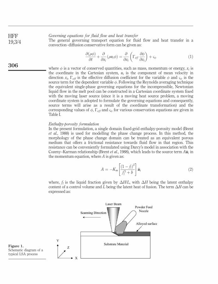
Mathematical formulationPhysical description of the problemThe physical problem involves melting of thin layer of a substrate with a continuousbeam laser moving with a constant scanning speed uscan in the negative x-direction andsimultaneously feeding an alloying element inside the laser generated melt pool (referto Figure 1). The intense heat from the laser beam creates a large temperature gradientin the substrate which induces a strong surface tension driven flow. As soon as thelaser moves resolidification occurs which leads to the final alloyed microstructure. Theflow and thermo-solutal histories are essential to predict the microstructuralcomposition and entropy generation in the process.

HFF19,3/4

306

Governing equations for fluid flow and heat transferThe general governing transport equation for fluid flow and heat transfer in aconvection–diffusion conservative form can be given as:

@ ��ð Þ@tþ @

@xi

�ui�ð Þ ¼ @

@xi

�eff

@�

@xi

� �þ &� ð1Þ

where � is a vector of conserved quantities, such as mass, momentum or energy, xi isthe coordinate in the Cartesian system, ui is the component of mean velocity indirection xi, �eff is the effective diffusion coefficient for the variable � and &� is thesource term for the dependent variable �. Following the Reynolds averaging techniquethe equivalent single-phase governing equations for the incompressible, Newtonianliquid flow in the melt pool can be constructed in a Cartesian coordinate system fixedwith the moving laser source (since it is a moving heat source problem, a movingcoordinate system is adopted to formulate the governing equations and consequently,source terms will arise as a result of the coordinate transformation) and thecorresponding values of �, �eff and &� for various conservation equations are given inTable I.

Enthalpy-porosity formulationIn the present formulation, a single domain fixed-grid enthalpy-porosity model (Brentet al., 1988) is used for modelling the phase change process. In this method, themorphology of the phase change domain can be treated as an equivalent porousmedium that offers a frictional resistance towards fluid flow in that region. Thisresistance can be conveniently formulated using Darcy’s model in association with theCozeny–Karman relationship (Brent et al., 1988), which leads to the source term A�uui inthe momentum equation, where A is given as:

A ¼ �Km1� flð Þ2

f 3l þ b

" #�uui ð2Þ

where, fl is the liquid fraction given by �H/L, with �H being the latent enthalpycontent of a control volume and L being the latent heat of fusion. The term �H can beexpressed as:

Figure 1.Schematic diagram of atypical LSA process

Entropygeneration

analysis

307

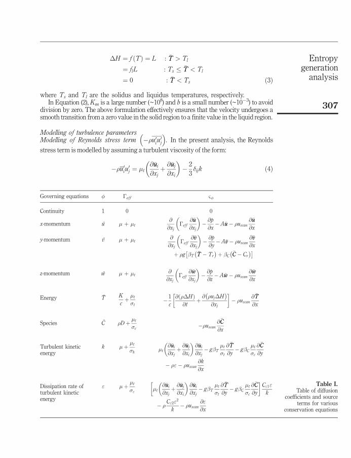
�H ¼ f ðTÞ ¼ L : �TT > Tl

¼ flL : Ts � �TT < Tl

¼ 0 : �TT < Ts ð3Þ

where Ts and Tl are the solidus and liquidus temperatures, respectively.In Equation (2), Km is a large number (~108) and b is a small number (~10�3) to avoid

division by zero. The above formulation effectively ensures that the velocity undergoes asmooth transition from a zero value in the solid region to a finite value in the liquid region.

Modelling of turbulence parametersModelling of Reynolds stress term ��u0iu

0j

� �. In the present analysis, the Reynolds

stress term is modelled by assuming a turbulent viscosity of the form:

��u0iu0j ¼ �t

@�uui

@xj

þ @�uuj

@xi

� �� 2

3�ijk ð4Þ

Governing equations � �eff &�

Continuity 1 0 0

x-momentum u � þ �t

@

@xj

�eff@�uu

@xj

� �� @p

@x� A�uu� �uscan

@�uu

@x

y-momentum v � þ �t@

@xj

�eff

@�vv

@xj

� �� @p

@y� A�vv� �uscan

@�vv

@x

þ �g �T�TT � Tr

� �þ �C

�CC � Cr

� ��

z-momentum w � þ �t@

@xj

�eff@�ww

@xj

� �� @p

@z� A�ww� �uscan

@�ww

@x

Energy T K

cþ �t

�t� 1

c

@ ��Hð Þ@t

þ@ �uj�H� �@xj

�� �uscan

@ �TT

@x

Species C �D þ �t

�c��uscan

@�CC

@x

Turbulent kineticenergy

k �þ �t

�k�t

@�uui

@xj

þ @�uuj

@xi

� �@�uui

@xj

� g�T�t

�t

@ �TT

@y� g�C

�t

�c

@�CC

@y

� �"� �uscan@k

@x

Dissipation rate ofturbulent kineticenergy

" �þ �t

�" �t@�uui

@xj

þ @�uuj

@xi

� �@�uui

@xj

� g�T�t

�t

@ �TT

@y� g�C

�t

�c

@�CC

@y

�C"1"

k

� �C"2"2

k� �uscan

@"

@x

Table I.Table of diffusion

coefficients and sourceterms for various

conservation equations

HFF19,3/4

308

where

�t ¼ffiffiffifl

pC��k2

"ð5Þ

In Equation (5), C� is a constant, whose value has been determined from shear-flowexperiments (Komatsu and Matsunaga, 1986). It is reported that C� varies from 0.08 to0.09 (Chen and Law, 1998). For the present study C� is taken to be 0.09. It is importantto note that in a standard high Reynolds number k� " model, the term

ffiffiffifl

pdoes not

appear. In the present problem, the whole domain is not composed of a single phaseso the formulation should ensure a reduction of eddy viscosity, thermal conductivityand mass diffusivity so that the effective diffusivity approaches to their respectivemolecular values along the solid–liquid interface, and merge with single-phaseturbulent flow conditions in the fully liquid region. It can be seen from Equation (5) theeddy viscosity goes to zero in the solid phase as liquid fraction is identically zero insolid and in liquid phase the eddy viscosity assumes the standard expression forsingle-phase flow problems as

ffiffiffifl

pis identically unity in liquid.

Modelling of turbulent heat flux ��u0iT0

� �. Following the same analogy as the

Reynolds stress, the turbulent heat flux (Reynolds heat flux) can be written as:

�u0iT0 ¼ t

@T

@xi

ð6Þ

where, t is the eddy thermal diffusivity. From the analogy of laminar flow, t can beexpressed as:

t ¼�t

��tð7Þ

where �t is turbulent Prandtl number. It has been proposed that �t varies from 0.8 to0.9.In the present work, �t ¼ 0.9.

Modelling of turbulent mass flux ð��u0iC0Þ. Following the same analogy as the

Reynolds stress, the turbulent mass flux (Reynolds mass flux) can be written as:

�u0iC0 ¼ c

@C

@xi

ð8Þ

where, c is the eddy mass diffusivity. From the analogy of laminar flow, c can beexpressed as:

c ¼�t

��cð9Þ

where, �c is turbulent Schmidt number. It has been proposed that �c varies from 0.8 to0.9.In the present work, �c ¼ 0.9.

Modelling evaporationA kinetic theory-based approach is adopted for modelling evaporation from the surfaceof the molten pool. The liquid surface layer formed by laser heating penetrates into the

Entropygeneration

analysis

309

solid at a rate determined by the quantity of vapour expelled. As the temperature of theliquid increases, the cohesive force in the liquid molecules decreases. As a result, thelatent heat of vaporization decreases with the temperature until the criticaltemperature is reached. The latent heat of vaporization can be given as:

Lv ¼ L0 1� TS

TC

� �2" #

ð10Þ

where L0 is the latent heat of vaporization at absolute zero and TS, TC are the surfacetemperature and critical temperature, respectively. The evaporating surface velocitycan be obtained from the surface velocity (Yilbas, 1997) as:

VS ¼kBT

2m

� �1=2

exp � Lv

kBT

� �ð11Þ

where m and kB are the mass per atom and Boltzmann constant, respectively.In the present model only heat loss due to vaporization is considered, however,

material reduction is not considered. The vaporization flux can be obtained from theevaporating surface velocity as:

J ¼ �vVS ¼PSVS

RTð12Þ

where, �v, PS are the density of the metal vapour and partial pressure, respectively.The net heat flux due to evaporation is given by JLv. In the calculations this amount

of heat loss from the top surface is added to heat loss due to other modes of heattransfer, i.e. convective heat loss, radiative heat loss. The vapour pressure is a functionof temperature and the function depends on the type of material.

Boundary conditionsThe boundary conditions for the thermal, solutal and flow variables with reference tothe work piece can be stated as follows:

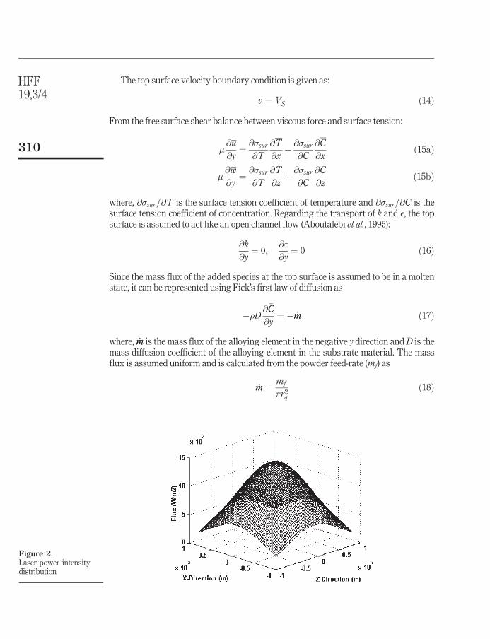
Top surfaceThe laser power intensity distribution is assumed to be Gaussian across the heatedspot, as shown in Figure 2. Considering convective, radiative and evaporative loss, theheat flux at the top surface can be given as:

�K@ �TT

@y

top

¼ � �Q

r2q

exp �f x2 þ z2� �

r2q

" #þ h �TT � T1� �

þ "r�rad�TT4 � T4

1� �

þ JLv

ð13Þ

where, Q is the total arc power, rq corresponds to the distance from the origin to thelocation where the power is reduced to 5 per cent of its maximum value, � is the powerefficiency, the sign of the heat flux corresponds to the heat flux is in negative ydirection, "r is the emissivity of the top surface and �rad is the Stefan–Boltzmannconstant.

HFF19,3/4

310

The top surface velocity boundary condition is given as:

v ¼ VS ð14Þ

From the free surface shear balance between viscous force and surface tension:

�@u

@y¼ @�sur

@T

@T

@xþ @�sur

@C

@C

@xð15aÞ

�@w

@y¼ @�sur

@T

@T

@zþ @�sur

@C

@C

@zð15bÞ

where, @�sur=@T is the surface tension coefficient of temperature and @�sur=@C is thesurface tension coefficient of concentration. Regarding the transport of k and �, the topsurface is assumed to act like an open channel flow (Aboutalebi et al., 1995):

@k

@y¼ 0;

@"

@y¼ 0 ð16Þ

Since the mass flux of the added species at the top surface is assumed to be in a moltenstate, it can be represented using Fick’s first law of diffusion as

��D@�CC

@y¼ � _mm ð17Þ

where, _mm is the mass flux of the alloying element in the negative y direction and D is themass diffusion coefficient of the alloying element in the substrate material. The massflux is assumed uniform and is calculated from the powder feed-rate (mf) as

_mm ¼ mf

r2q

ð18Þ

Figure 2.Laser power intensitydistribution

Entropygeneration

analysis

311

Side facesThe four side faces are subjected to convective heat transfer boundary condition:

�K@T

@n¼ hðTwall � TÞ ð19Þ

where, n is the direction of outward normal to the surface concerned and h is theconvective heat transfer coefficient.

Bottom facesThe face being insulated, the temperature boundary condition is:

@T

@y¼ 0 ð20Þ

Solid–liquid interfaceRegarding interface conditions, it is apparent that the solid/liquid interface in thisproblem acts as a wall, and the same needs to be treated appropriately. However,according to the enthalpy-porosity formulation, one does not need to track the interfaceseparately and impose velocity or temperature boundary conditions on the same, sincethe interface comes out as a natural outcome of the solution procedure itself. However,the evolving interface locations are important inputs for k and " equations, since thevalues of k and " are to be specified for near wall points with the help of suitable wallfunctions, which lead to satisfaction of the following conditions at the solid/liquidinterface:

k ¼ 0 ð21aÞ@"

@n¼ 0 ð21bÞ

It can be noted here that the alloying element added to the pool subsequently mixeswith the molten base metal by convection and diffusion. However, at the solidificationinterface, only a part of solute kp

�CC goes into the solid phase, where kp is the partitioncoefficient. Thus, the solute flux balance at the solidification front is given by(Flemings, 1974):

�D@�CC

@n¼ vn

�CCð1� kpÞ ð22aÞ

where n is the direction of outward normal, and vn is the interface velocity in thatdirection. Similarly, the boundary condition at the fusion front can be written as(Flemings, 1974):

�D@�CC

@n¼ vn

�CC ð22bÞ

HFF19,3/4

312

Entropy generation analysisThe entropy generation is estimated following the solution of entropy transportequation along with entropy boundary conditions.

Second law as a transport equationThe second law for an equivalent single-phase can be represented in a form similar toEquation (1), but it includes an inequality, rather than equality, because entropy istypically produced, rather than only conserved.

_PPs �@S

@tþr �� � 0 ð23Þ

where _PPs; S and � are the entropy production rate, entropy and the entropy flux,respectively. Expressing the entropy flux in terms of advective and diffusivecomponents, Equation (23) becomes:

D �sð ÞDt¼ r � KrT

T

� �þr �

Xi

gi_JJi

T

!þ _PPs ð24Þ

where s, gi and _JJi are specific entropy, chemical potential and species flux ofconstituent i.

Local rate of entropy productionInvoking the Gibbs equation and the entropy transport equation (Naterer and Roach,1998), the general expression for the rate of local entropy generation in a flow field withboth heat and mass transfer can be written as:

_PPs ¼K

T2rTð Þ2þ �

T�� 1

T

Xi

_JJi � rgi þ1

T2

Xi

gi_JJi � rT ð25Þ

where, � represents the viscous dissipation for a convective flow. For a three-dimensional situation � is given as:

� ¼ 2@u

@x

� �2

þ @v

@y

� �2

þ @w

@z

� �2" #

þ @v

@xþ @u

@y

�2

þ @w

@yþ @v

@z

�2

þ @u

@zþ @w

@x

�2

� 2

3

@u

@xþ @v

@yþ @w

@z

�2

ð26Þ

From Fick’s law of mass diffusion, the species flux of i-th species can be given by�DirCi where, Di is the mass diffusion coefficient of the i-th species. The chemicalpotential gradient can be rewritten asrgi � rCi.

Entropygeneration

analysis

313

Total entropy generation and entropy generation numberThe total entropy generation is calculated as follows:

Ps ¼ððð

V

�sdV ð27Þ

The first law efficiency of the process may be written as:

�I ¼Actual energy stored in the system

Energy supplied the system by laser beam¼

ÐÐÐV

� cT þ�Hð Þ dV

�Q �tð28Þ

where, � is the efficiency of laser heating, Q represents the total laser power and �t isthe laser heating time. From the definition, the first law efficiency can be viewed as aratio of two energies and it reflects the energy losses as a low-grade heat.

For description of the second law efficiency, the entropy generation number (Bejan,1987) needs to be introduced.

Ns ¼Total availability destroyed during the process

Total availability that enters the system during the process¼ T0Ps

�Qð29Þ

where T0 is the initial temperature of the substrate material.Following the above description of the entropy generation number, the second law

efficiency may be expressed as:

�II ¼ 1� Ns ð30Þ

Numerical implementationDiscretization of conservation equationsThe governing equations are discretized using the control volume method, where awhole rectangular computational domain is divided into small rectangular controlvolumes. A scalar grid point is located at the centre of each control volume, storing thevalues for scalar variables such as pressure, enthalpy and entropy. In order to ensurethe stability of numerical calculation, velocity components are arranged on differentgrid points, staggered with respect to scalar grid points. Discretized equations for avariable are formulated by integrating the corresponding governing equation over thethree-dimensional control volumes. The final discretized equation takes the followingform (Patankar, 1980):

aP�P ¼Xnb

anb�nbð Þ þ a0P�

0P þ &U �V ð31Þ

where, subscript P represents a given grid point, while subscript nb represents theneighbours of the given grid point P, � is a general variable such as velocity orenthalpy, a is the coefficient calculated based on the power law scheme, �V is thevolume of the control volume, a0

P and �0P are the coefficient and value of the general

variable at the previous time step, respectively. The coefficient aP is defined as:

HFF19,3/4

314

aP ¼Xnb

anb þ a0P � &P�V ð32Þ

The terms &U and &P are used in the source term linearization as:

& ¼ &U þ &P�P ð33Þ

The coupled conservation equations are then solved iteratively on a line-by-line basisusing a tri-diagonal matrix algorithm following a pressure-based finite volume methodaccording to the SIMPLER algorithm (Patankar, 1980). The latent heat content of eachcontrol volume is updated using the temperature field obtained from energy equation,as outlined in Brent et al. (1988).

Discretization of second law of thermodynamicsIntegrating Equation (23) over a control volume and time step, one can write

ðV

ðtþ�t

t

@S

@tdt dV þ

ðtþ�t

t

ðV

r ��ð ÞdV dt � 0 ð34Þ

Performing the integration in Equation (34) for a discrete volume �V and following animplicit formulation over the time step �t ¼ tnþ1 � tn, one obtains:

_PPs �Snþ1

i � Sni

�t

!�V þ

Xnb

�nb

" #nþ1

� 0 ð35Þ

The Gibbs equation is invoked here to represent the transient entropy derivative inEquation (35) in terms of variables obtained from solution of the conservationequations, such as temperature and liquid fraction.

Snþ1i � Sn

i

�t¼ �c

Tni

Tnþ1i � Tn

i

�t

!þ ��Sf

f nþ1l;i � f n

l;i

�t

!ð36Þ

where, �Sf ¼ sl � ss refers to the entropy of fusion (approximately equal to the heat offusion divided by the phase change temperature).

Discretization of entropy equation of stateAn entropy equation of state is also required for the implementation of the second law.Considering entropy as a function of temperature and concentration a piecewiselogarithmic equation of state following Gibbs equation for an incompressiblesubstance is assumed.

s T;Cð Þ ¼ sr;k þ Cr;k lnT

Tr;k

� �ð37Þ

where, the subscripts r and k denote reference and phase respectively. The followingreference values are used depending on the computed value of the liquid fraction.

Entropygeneration

analysis

315

sr;s ¼ 0

Cr;s ¼ Cs

Tr;s ¼ Te

9>=>; for fl ¼ 0

sr;m ¼ Cs ln Ts=Teð Þ

Cr;m ¼CsTl � ClTs

Tl � Ts

� �þ Cl � Cs þ�Sf

ln Tl=Tsð ÞTr;m ¼ Ts

9>>>=>>>;

for 0 < fl < 1 ð38Þ

sr;l ¼CsTl � ClTs

Tl � Ts

� �ln

Tl

Ts

� �þ Cs ln

Ts

Te

� �þ Cl � Cs þ�Sf

Cr;l ¼ Cl

Tr;l ¼ Tl

9>>>=>>>;

for fl ¼ 1

where, the subscripts s, l, m and e denote the solid, liquid, mushy (two-phase) regionand eutectic composition.

Entropy boundary conditionIntroducing the entropy equation of state closes the entropy equations for interiorcontrol volumes. However, closure is still required for the boundary control volumes.The inflow and outflow of entropy are required to be computed for closure of thesecond law in the boundary control volumes.

The boundary entropy production rate is directly computed from Equation (25)using the spatial derivatives of temperature, velocity and concentration. The interfacialentropy balance can be given as:

Ps;i ¼�s

�l

�Sf �L

T

� �þ Kl

�lVl

dT

dn

l

1

Tl

� 1

Ts

� �� 0 ð39Þ

Grid spacing and time stepIn order to capture the top surface velocity originating from surface tension gradients,the choice of grid-size should be judicious. This also ensures indirectly that thecalculations for velocity gradients are accurate enough, so that the turbulent sourceterms can be properly evaluated. In order to capture sufficient flow details inside thesurface tension driven boundary layer at the top surface, at least a few (typically five)grid points are accommodated inside the same. In order to specify the diffusioncoefficients near the wall using wall conditions (Chen and Law, 1998), it is necessary tocontrol the grid size in the vicinity. Otherwise, it can be possible that the grid pointsimmediately next to the wall will fall beyond the ‘‘near wall’’ regime. Accordingly, wechoose a depth of 4.0 � 10�6 m for the topmost grids. Just below this, the grid depthsare taken as 8.0 � 10�6 m, followed by a depth of three grid spacing of 1.2 � 10�5 m.Then 2.4 � 10�5 m, 4.1 � 10�5 m, 4.9 � 10�5 m, 5.3 � 10�5 m and 9.8 � 10�5 m,respectively, in negative y direction. Thereafter a uniform grid depth of 3.75 � 10�4 mis employed for most of the remaining part of the pool. The grid spacing is madecoarser in y-direction gradually. Outside the molten pool, a non-uniform coarse grid ischosen. In the x and z direction, an optimized grid size near the wall is found to be

HFF19,3/4

316

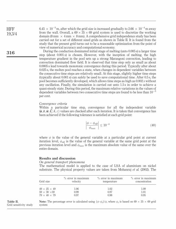
6.45 � 10�5 m, after which the grid size is increased gradually to 2.66 � 10�4 m awayfrom the wall. Overall, a 69� 35� 69 grid system is used to discretize the workingdomain (8 mm � 4 mm � 8 mm). A comprehensive grid independence study has beencarried out for a set of different sized grids as shown in Table II. It is found from thestudy that the present grid turns out to be a reasonable optimization from the point ofview of numerical accuracy and computational economy.

During the conduction dominated initial stage of melting (unto 0.005 s) a larger timestep (about 0.001 s) is chosen. However, with the inception of melting, the hightemperature gradient in the pool sets up a strong Marangoni convection, leading toconvection dominated flow field. It is observed that time step only as small as about0.0005 s lead towards monotonic convergence during this period. Typically after about0.025 s, the molten pool reaches a state, when changes in dependent variables betweenthe consecutive time steps are relatively small. At this stage, slightly higher time steps(typically about 0.001 s) can safely be used to save computational time. After 0.5 s, thepool becomes sufficiently developed, which allows time steps as high as 0.002 s withoutany oscillation. Finally, the simulation is carried out unto 1.5 s in order to achieve aquasi-steady state. During this period, the maximum relative variations in the values ofdependent variables between two consecutive time steps are found to be less than 10�5

per cent.

Convergence criteriaWithin a particular time step, convergence for all the independent variable(�uu;�vv; �ww; �CC; k; "Þ values are checked after each iteration. It is taken that convergence hasbeen achieved if the following tolerance is satisfied at each grid point:

�� �old

�max

� 10�4 ð40Þ

where � is the value of the general variable at a particular grid point at currentiteration level, �old is the value of the general variable at the same grid point at theprevious iteration level and �max is the maximum absolute value of the same over theentire domain.

Results and discussionOn general transport phenomenaThe mathematical model is applied to the case of LSA of aluminium on nickelsubstrate. The physical property values are taken from Mohanraj et al. (2002). The

Table II.Grid sensitivity study

Grid size% error in maximum

velocity% error in maximum

temperature% error in maximum

concentration

49 � 25 � 49 1.06 1.02 1.0959 � 30 �59 0.99 0.97 1.0179 � 40 � 79 0.97 0.98 0.95

Note: The percentage error is calculated using {�–�z}/�, where �z is based on 69 � 35 � 69 gridsystem

Entropygeneration

analysis

317

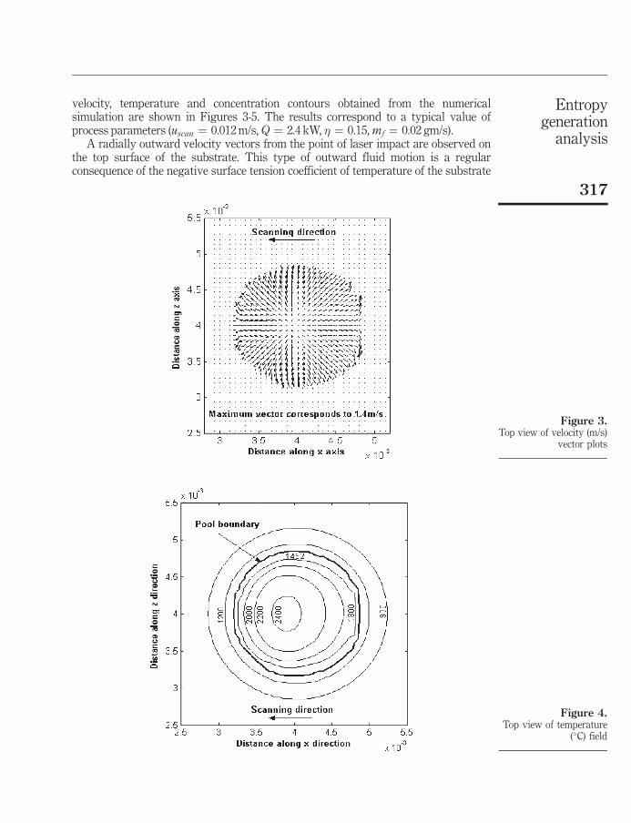
velocity, temperature and concentration contours obtained from the numericalsimulation are shown in Figures 3-5. The results correspond to a typical value ofprocess parameters (uscan ¼ 0.012 m/s, Q ¼ 2.4 kW, � ¼ 0.15, mf ¼ 0.02 gm/s).

A radially outward velocity vectors from the point of laser impact are observed onthe top surface of the substrate. This type of outward fluid motion is a regularconsequence of the negative surface tension coefficient of temperature of the substrate

Figure 3.Top view of velocity (m/s)

vector plots

Figure 4.Top view of temperature

(C) field

HFF19,3/4

318

material. It should be mentioned here that the liquid flow is mainly driven by surfacetension force and to a much less extent by the buoyancy force. This fact can besupplemented by a dimensional analysis. The ratio of buoyancy force to viscous forceis determined by Grashof number, which is given as:

Gr ¼ GrT þ GrC ¼g�T�Tl3ref ;t�

2

�2þ

g�C�Cl3ref ;c�2

�2ð41Þ

where GrT and GrC are the thermal and solutal Grashof numbers, �T and �C are thetemperature and concentration differences between the peak values and the

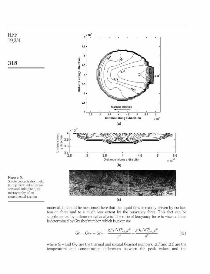
Figure 5.Solute concentration field:(a) top view, (b) at cross-sectional mid-plane, (c)micrography of anexperimental section

Entropygeneration

analysis

319

corresponding eutectic values and lref ;t and lref ;c are the characteristic lengths whichare chosen to be the thermal and concentration boundary layer thicknesses,respectively. The surface tension Reynolds number or the Marangoni number (Ma) isgiven by the ratio of surface tension gradient force to viscous force as:

Ma ¼ �lref ;v�T @�sur=@Tj j�2

þ �lref ;c�C @�sur=@Cj j�2

ð42Þ

where lref ;v is the characteristic length given by the viscous boundary layer thickness.Using the physical properties from Mohanraj et al. (2002), the corresponding values

of Grashof and Marangoni numbers are estimated as 0.8195 and 10950.5. The ratio ofsurface tension force to buoyant force is expressed as:

Rs=b ¼Ma

Gr¼ 10950:5

0:8195¼ 1:336� 104 ð43Þ

Hence, it can be concluded that the liquid flow is mainly induced by the Marangoniconvection and to a lesser extent by the buoyancy force.

The temperature contours as observed from Figure 4, are almost concentric circles.This type of geometry is a consequence of the anisotropic nature of an enhanceddiffusion process in case of turbulent molten pool. In the present case, the net thermalenergy available to the pool is predominantly transported along the longitudinal andsidewise directions by the Marangoni advection along with molecular as well as eddythermal diffusion process. The downward advection of heat is small compared tolongitudinal and span wise advection because of much smaller magnitude ofdownward velocity component, as compared to magnitudes of longitudinal and spanwise components. In case of turbulent transport, due to an enhanced mixing process onaccount of an efficient energy cascading mechanism taking place betweenparticipating eddies, the mean advection strength goes down, which results in adecrease in longitudinal and sidewise advection strength. On the other hand, anenhanced effective diffusion process due to interactions between fluctuating velocitycomponents of eddies in a turbulent pool tries to increase the length and width of thepool by propagating the influence of thermal disturbance across a relatively largerdistance. The resultant pool geometry is, therefore, a consequence of the above twocounteracting effects active in tandem.

The distribution of aluminium concentration in the molten pool is shown in Figure 5.It is evident from the above figure that the concentration of solute is higher near thesolidification front and gradually decreases toward the melting front. At the meltingfront, dilution of species takes place due to fresh addition of molten base metal. On thecontrary, since solubility of the solute in the solid phase is less than that in the liquidphase for the present case, there will be preferential solute rejection from the solidifiedmaterial back into the molten pool at the solidification front. The rejected solute istransported back into the centre of the pool as a consequence of the combinedadvection-diffusion field.

It is apprehended that the simulation results of the transport processes occurringinside the laser molten pool can provide better insight of the nature of microstructurethat would be expected. As a visual appreciation a micrography of an experimentalsection (Mohanraj et al., 2002) is shown in Figure 5(c) along with the numerically

HFF19,3/4

320

obtained solute concentration distribution at the cross-sectional mid-plane. Thecomparison shows an excellent experimental agreement of the present model and alsodemonstrates the capability of the model to predict the nature of the evolvedmicrostructure.

On entropy generationThe total entropy generation consists of entropy generation due to heat transfer, masstransfer, fluid friction and combined heat and mass transfer. However, entropygeneration due to heat transfer is found to contribute about 99 per cent of the total

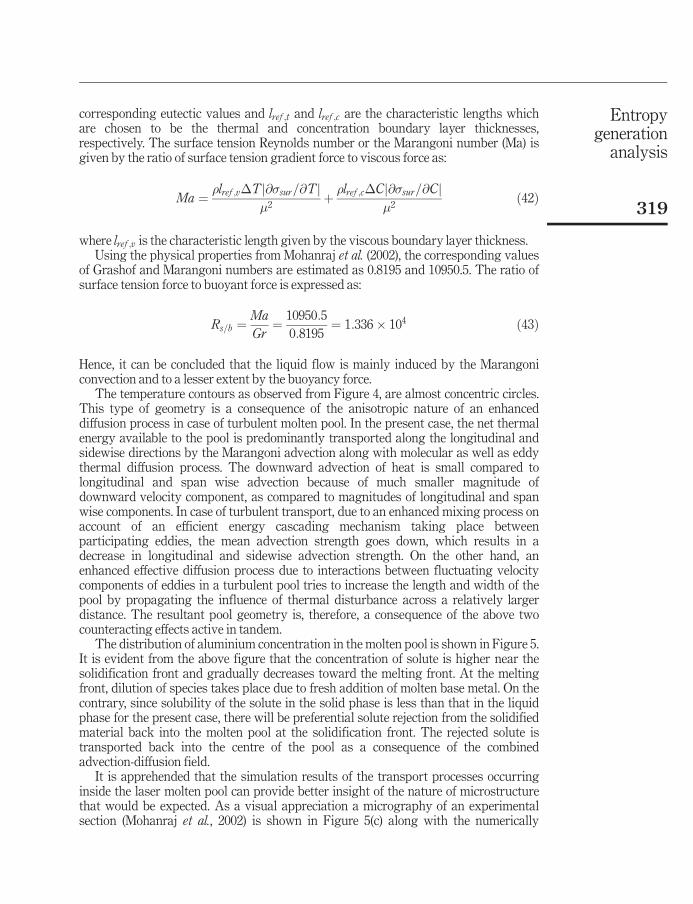
Figure 6.Variation of temperaturewith time in alongitudinal section alongthe direction of laserscanning

Figure 7.Variation of cooling ratewith time in alongitudinal section alongthe direction of laserscanning

Entropygeneration

analysis

321

entropy generation. Hence, it is important to observe the temperature response of thesubstrate material due to laser heating on the context of entropy generation.

Figure 6 shows the temporal variation of the top surface temperature in alongitudinal section along the direction of laser scanning. The curve shows a steepergradient near the melting front than near the solidification front. Also, beneath the tip

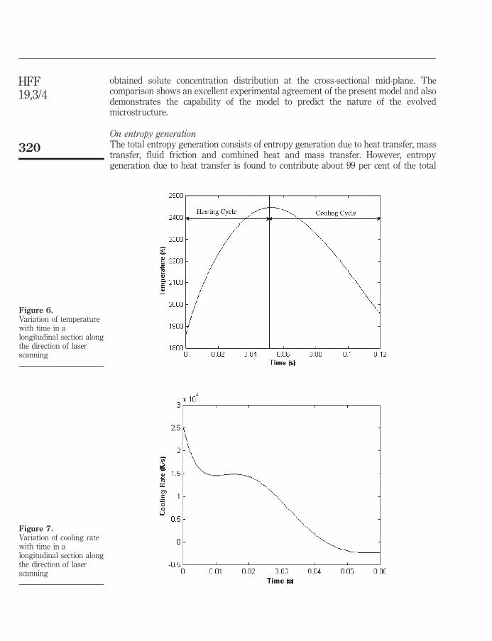
Figure 8.(a) Temperature variation

along x-axis on the topsurface, (b) variation of

dT/dx along x-axis on thetop surface

HFF19,3/4

322

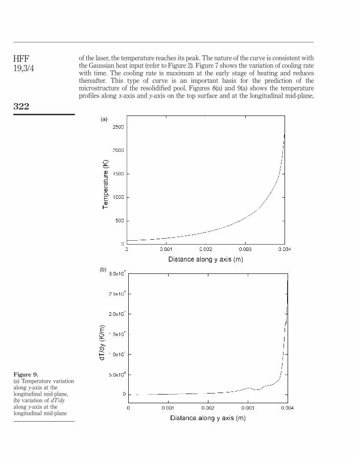
of the laser, the temperature reaches its peak. The nature of the curve is consistent withthe Gaussian heat input (refer to Figure 2). Figure 7 shows the variation of cooling ratewith time. The cooling rate is maximum at the early stage of heating and reducesthereafter. This type of curve is an important basis for the prediction of themicrostructure of the resolidified pool. Figures 8(a) and 9(a) shows the temperatureprofiles along x-axis and y-axis on the top surface and at the longitudinal mid-plane,

Figure 9.(a) Temperature variationalong y-axis at thelongitudinal mid-plane,(b) variation of dT/dyalong y-axis at thelongitudinal mid-plane

Entropygeneration

analysis

323

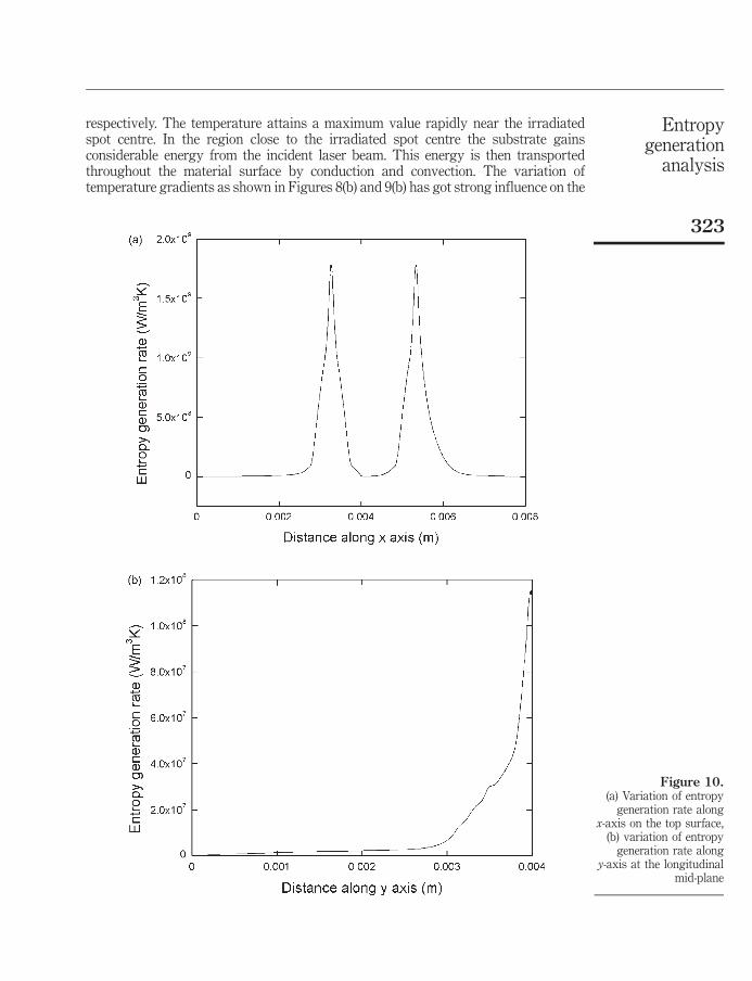
respectively. The temperature attains a maximum value rapidly near the irradiatedspot centre. In the region close to the irradiated spot centre the substrate gainsconsiderable energy from the incident laser beam. This energy is then transportedthroughout the material surface by conduction and convection. The variation oftemperature gradients as shown in Figures 8(b) and 9(b) has got strong influence on the

Figure 10.(a) Variation of entropy

generation rate alongx-axis on the top surface,

(b) variation of entropygeneration rate along

y-axis at the longitudinalmid-plane

HFF19,3/4

324

entropy production rate. The local entropy production rate is directly proportional tothe square of the temperature gradient. In Figure 8(b) the temperature gradient isfound to be symmetrical about the central cross-sectional plane, which ensures that theentropy production rate will also be symmetrical about the same plane as shown inFigure 10(a). Figure 9(b) shows that the maximum variation of temperature gradient islimited to a thin layer from the top surface of the substrate material. This is due to thefact that the main mode of heat transfer in the vertical direction is conduction. Asexpected the entropy generation rate curve along y-axis (Figure 10(b)) shows the samenature qualitatively with the temperature gradient. Further, spikes in the temperaturegradient at the edges of the molten pool are observed which can be attributed by thefact that the main mode of heat transfer in the molten pool is convection whereasoutside the molten pool it is conduction. Hence there is a drastic change of thetemperature gradient at the edge of the molten pool and accordingly the spikes areobserved.

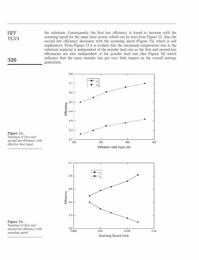
On efficiency analysisThe variations of first law and second law efficiency with effective heat input, scanningspeed and powder feed rate are shown in Figures 14-16. The maximum first lawefficiency is found to be around 0.7, which is considerably high, whereas the maximumsecond law efficiency is around 0.3. This indicates that the useful work done on thesubstrate material is considerably less. The nature of variation of efficiency can beexplained with the help of the nature of variation of temperature as shown in Figures11-13. In Figure 11 shown the variation of maximum temperature with effective heatinput. The temperature is expected to increase with the heat input, as the internalenergy gain of the workpiece increases with the laser power input. As a consequence ofthe substantial increase in the internal energy gain of the substrate, the first lawefficiency increases as evident from Figure 14. The total availability that destroyedduring the process as well as the total availability that enters the system increase withthe increase in maximum temperature or effective heat input. However, the rate of

Figure 11.Variation of maximumtemperature with effectiveheat input

Entropygeneration

analysis

325

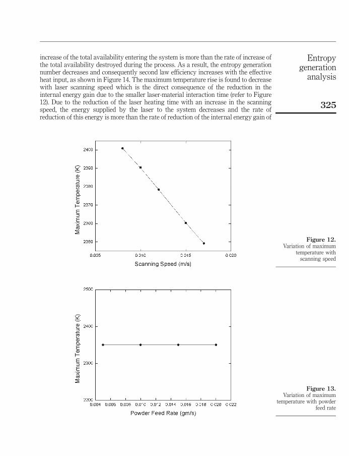
increase of the total availability entering the system is more than the rate of increase ofthe total availability destroyed during the process. As a result, the entropy generationnumber decreases and consequently second law efficiency increases with the effectiveheat input, as shown in Figure 14. The maximum temperature rise is found to decreasewith laser scanning speed which is the direct consequence of the reduction in theinternal energy gain due to the smaller laser-material interaction time (refer to Figure12). Due to the reduction of the laser heating time with an increase in the scanningspeed, the energy supplied by the laser to the system decreases and the rate ofreduction of this energy is more than the rate of reduction of the internal energy gain of

Figure 12.Variation of maximum

temperature withscanning speed

Figure 13.Variation of maximum

temperature with powderfeed rate

HFF19,3/4

326

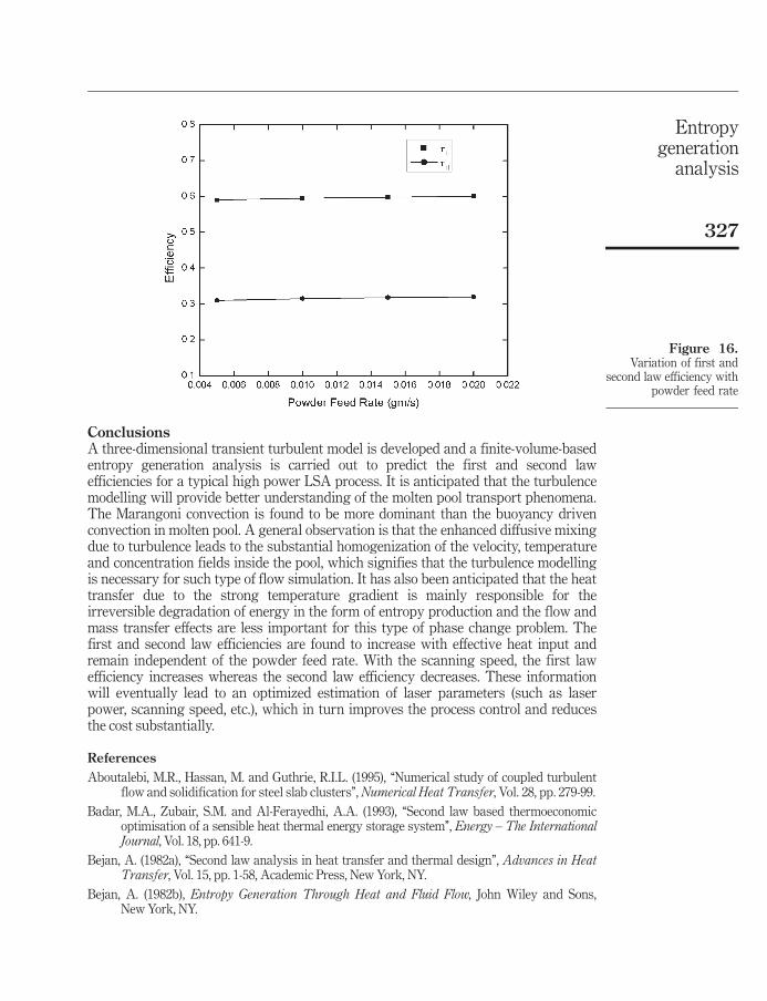
the substrate. Consequently, the first law efficiency is found to increase with thescanning speed for the same laser power, which can be seen from Figure 15. Also thesecond law efficiency decreases with the scanning speed (Figure 15), which is selfexplanatory. From Figure 13 it is evident that the maximum temperature rise in thesubstrate material is independent of the powder feed rate as the first and second lawefficiencies are also independent of the powder feed rate (See Figure 16) whichindicates that the mass transfer has got very little impact on the overall entropygeneration.

Figure 14.Variation of first andsecond law efficiency witheffective heat input

Figure 15.Variation of first andsecond law efficiency withscanning speed

Entropygeneration

analysis

327

ConclusionsA three-dimensional transient turbulent model is developed and a finite-volume-basedentropy generation analysis is carried out to predict the first and second lawefficiencies for a typical high power LSA process. It is anticipated that the turbulencemodelling will provide better understanding of the molten pool transport phenomena.The Marangoni convection is found to be more dominant than the buoyancy drivenconvection in molten pool. A general observation is that the enhanced diffusive mixingdue to turbulence leads to the substantial homogenization of the velocity, temperatureand concentration fields inside the pool, which signifies that the turbulence modellingis necessary for such type of flow simulation. It has also been anticipated that the heattransfer due to the strong temperature gradient is mainly responsible for theirreversible degradation of energy in the form of entropy production and the flow andmass transfer effects are less important for this type of phase change problem. Thefirst and second law efficiencies are found to increase with effective heat input andremain independent of the powder feed rate. With the scanning speed, the first lawefficiency increases whereas the second law efficiency decreases. These informationwill eventually lead to an optimized estimation of laser parameters (such as laserpower, scanning speed, etc.), which in turn improves the process control and reducesthe cost substantially.

References

Aboutalebi, M.R., Hassan, M. and Guthrie, R.I.L. (1995), ‘‘Numerical study of coupled turbulentflow and solidification for steel slab clusters’’, Numerical Heat Transfer, Vol. 28, pp. 279-99.

Badar, M.A., Zubair, S.M. and Al-Ferayedhi, A.A. (1993), ‘‘Second law based thermoeconomicoptimisation of a sensible heat thermal energy storage system’’, Energy – The InternationalJournal, Vol. 18, pp. 641-9.

Bejan, A. (1982a), ‘‘Second law analysis in heat transfer and thermal design’’, Advances in HeatTransfer, Vol. 15, pp. 1-58, Academic Press, New York, NY.

Bejan, A. (1982b), Entropy Generation Through Heat and Fluid Flow, John Wiley and Sons,New York, NY.

Figure 16.Variation of first and

second law efficiency withpowder feed rate

HFF19,3/4

328

Bejan, A. (1987), ‘‘The thermodynamic design of heat and mass transfer process and devices’’,Heat and Fluid Flow, Vol. 8, pp. 258-76.

Brent, A.D., Voller, V.R. and Reid, K.J. (1988), ‘‘Enthalpy-porosity technique for modellingconvection-diffusion phase change: application to the melting of a pure metal’’, NumericalHeat Transfer, Vol. 13, pp. 297-318.

Chen, C.J. and Law, S.Y. (1998), Fundamentals of Turbulence Modelling, Taylor & Francis,Philadelphia, PA.

Flemings, M.C. (1974), Solidification Processing, McGraw-Hill, New York, NY.

Haddad, O.M., Abu-Qudais, M., Abu-Hijleh, B. and Maqableh, A.M. (2000), ‘‘Entropy generationdue to laminar forced convection flow past a parabolic cylinder’’, International Journal ofNumerical Methods for Heat and Fluid Flow, Vol. 10, pp. 770-9.

Komatsu, T. and Matsunaga, N. (1986), ‘‘Defect of "�k turbulence model and its improvements’’,Proceedings of 30th Japan Conference on Hydraulics, pp. 529-34.

Krane, B.J. (1985), ‘‘A second law analysis of a thermal energy storage with Joulean heating of thestorage element’’, ASME paper 85-WA/HT-19.

Krane, B.J. (1987), ‘‘A second law analysis of the optimum design and operation of thermal energystorage systems’’, International Journal of Heat Mass Transfer, Vol. 30, pp. 43-57.

Mathiprakasam, B. and Beeson, J. (1984), ‘‘Second law analysis of thermal energy storagedevices’’, Heat transfer-Seattle, AIChE Symposium Series, pp. 161-8.

Mohanraj, P., Sarkar, S., Chakraborty, S., Phanikumar, G., Dutta, P. and Chattopadhyay, K. (2002),‘‘Modelling of transport phenomena in laser surface alloying with distributed species masssource’’, International Journal of Heat and Fluid Flow, Vol. 23, pp. 298-307.

Naterer, G.F. and Roach, D.C. (1998), ‘‘Entropy and numerical stability in phase change problems’’,AIAA paper 98-2765, AIAA/ASME 7th Joint Thermophysics and Heat TransferConference, Albuquerque, NM, 15-18 June.

Patankar, S.V. (1980), Numerical Heat Transfer and Fluid Flow, Hemisphere, Washington DC.

Shuja, S.Z., Yilbas, B.S. and Budair, M.O. (2002), ‘‘Investigation into a confined laminar swirlingjet and entropy production’’, International Journal of Numerical Methods for Heat andFluid Flow, Vol. 12, pp. 870-87.

Shuja, S.Z., Yilbas, B.S. and Budair, M.O. (2007), ‘‘Entropy generation due to jet impingement on asurface: effect of annular nozzle outer angle’’, International Journal of Numerical Methodsfor Heat and Fluid Flow, Vol. 17, pp. 677-91.

Yilbas, B.S. (1997), ‘‘Laser heating process and experimental validation’’, International Journal ofHeat Mass Transfer, Vol. 40, pp. 1131-43.

Yilbas, B.S. (1999), ‘‘Three-dimensional laser heating model and entropy generationconsideration’’, Journal of Energy Resources Technology, Vol. 121, pp. 217-24.

Corresponding authorDipankar Chatterjee can be contacted at: rsdchat@yahoo.co.in

To purchase reprints of this article please e-mail: reprints@emeraldinsight.comOr visit our web site for further details: www.emeraldinsight.com/reprints