36
No 38 Entry Deterrence Through Cooperative R&D Over-Investment Clémence Christin November 2011
No 38
Entry Deterrence Through Cooperative R&D Over-Investment Clémence Christin
November 2011

IMPRINT DICE DISCUSSION PAPER Published by Heinrich‐Heine‐Universität Düsseldorf, Department of Economics, Düsseldorf Institute for Competition Economics (DICE), Universitätsstraße 1, 40225 Düsseldorf, Germany Editor: Prof. Dr. Hans‐Theo Normann Düsseldorf Institute for Competition Economics (DICE) Phone: +49(0) 211‐81‐15125, e‐mail: [email protected]‐duesseldorf.de DICE DISCUSSION PAPER All rights reserved. Düsseldorf, Germany, 2011 ISSN 2190‐9938 (online) – ISBN 978‐3‐86304‐037‐6 The working papers published in the Series constitute work in progress circulated to stimulate discussion and critical comments. Views expressed represent exclusively the authors’ own opinions and do not necessarily reflect those of the editor.
Entry Deterrence Through Cooperative
R&D Over-Investment
Clémence Christin∗
November 2011
Abstract
In this paper, we highlight new conditions under which R&D agreements
may have anti-competitive e�ects. We focus on cases where two �rms compete
with each other and with a competitive fringe. R&D activities need a speci�c
input available to all �rms on a common market, the price of which increases
with demand for the input. In such a context, if a �rm increases its R&D
expenses, it increases the cost of R&D for its rivals. This induces exit from
the fringe and may increase the �nal price. Therefore, by contrast to the case
where the cost of R&D for one �rm is independent of its rivals' R&D decisions,
cooperation between strategic �rms on the upstream market may induce more
R&D by strategic �rms, in order to exclude �rms from the fringe and increase
the �nal price.
JEL Classi�cations: L13, L24, L41.
Key words: Competition policy, Research and Development Agreements, Col-
lusion, Entry deterrence.
∗Düsseldorf Institute for Competition Economics (DICE), Heinrich Heine Universität, Gebäude
24.31, Universitätsstr. 1, 40225 Düsseldorf, Germany; [email protected], tel: +49
211 81 10 233. Support from the Düsseldorf Institute for Competition Economics (DICE) and from
the French-German cooperation project �Market Power in Vertically Related Markets� funded by
the Agence Nationale de la Recherche (ANR) and the Deutsche Forschungsgemeinschaft (DFG) is
gratefully acknowledged. I would like to thank Marie-Laure Allain, Eric Avenel, Claire Chambolle,
Patrick DeGraba, Bruno Jullien, Laurent Linnemer, Guy Meunier, Matias Nunez, Jean-Pierre
Ponssard, Patrick Rey and Bernard Sinclair-Desgagné, as well as participants at IIOC 2010, EARIE
2010 and JMA 2010 conferences for very useful comments.
1
1 Introduction
Horizontal agreements in general are forbidden by Article 101 of the Treaty on
the Functioning of the European Union because of their anti-competitive e�ects.
Research and development (R&D) agreements however are considered to create ef-
�ciency gains that are likely to o�set their potential anti-competitive e�ects, and
consequently bene�t from a �block exemption� as long as the market share of par-
ticipants is lower than 25%. Even R&D agreements involving �rms with a total
market share higher than 25% may be allowed.1
The anti-competitive concerns of the EU Competition Commission as well as US
antitrust authorities regarding R&D agreements are essentially of three types:2 First,
�rms may want to engage in R&D agreements in order to slow down R&D e�orts and
reduce variety on the �nal market. Second, R&D cooperation may be transferred
to other markets and lead to increased �nal prices. Finally, R&D agreements may
lead to market foreclosure. The main concern of competition authorities is thus the
direct restriction of competition on the �nal market that may result from an R&D
agreement. Less attention however is given to the indirect e�ect of R&D agreements
on competition through the market for inputs necessary for R&D.
In this paper, we highlight one speci�c means through which an R&D agreement
may indirectly deter entry on the �nal market through entry deterrence on the mar-
ket for R&D inputs. We also show that R&D agreements may be anti-competitive
even when members of the R&D agreement increase their R&D e�orts. Indeed,
when �rms must compete to purchase some inputs necessary for R&D, members of
the agreement may increase their R&D e�orts only to increase the cost of R&D for
their rivals, hence reducing competition on the �nal market. Although increasing
R&D also increases the e�ciency of the members of the agreement, this second e�ect
may be o�set by the former.
Besides often competing on the same �nal market, �rms engaging in (similar)
R&D activities need inputs for which they also have to compete, the main example of
which is skilled workers. According to a survey by the US National Science Founda-
1See the Guidelines on the applicability of Article 101 of the EC Treaty on the Functioning ofthe European Union to horizontal cooperation agreements, O�cial Journal of the European Union,2011.
2See again the European Guidelines (2011) and the Antitrust Guidelines for CollaborationsAmong Competitors issued by the Federal Trade Commission and the US Department of Justice(April 2000).
2

tion, wages and related labor costs accounted for more than 40% of the US industrial
R&D costs in the 1990s, and for 46.6% in 2006. Although this hides a relative vari-
ety among industries, labor-related costs are a particularly large part of R&D costs
in large R&D consuming industries such as pharmaceuticals and medicine (where
labor costs represent 28.8% of all R&D costs), computer and electronic products
(51.9%), computer systems designing (55.3%) and information (62%).3 Parallel to
this, concerns are often raised both by �rms in innovative markets and by govern-
ments as to the need for more research personnel.4 High skilled labor, especially
labor in the science and technology �elds typically needed for R&D activities is
usually characterized by signi�cantly lower unemployment rates than other types of
labor, and some countries such as Germany have su�ered from skills shortage in the
past years.5
Given the more or less stringent capacity constraint on skilled labor, one can
then argue that R&D costs of �rms engaging in similar R&D activities are not as
independent from one another as is usually assumed.6 Then, there exists a risk that
�rms with enough market power on the market for R&D inputs manage to prevent
the entry of �rms with less market power on this market. This is a particularly
legitimate concern in R&D intensive industries, as they are often characterized by
large size asymmetries between the �rms. Focusing for example on the biotech-
nology industry, one can �nd at di�erent levels of the innovation and production
process large pharmaceutical companies competing with medium sized to very small
biotechnology companies. The IT services industry is characterized by the same
type of market structure: in 2001, while only 0.2% of the IT service companies in
3National Science Foundation, National Center for Science and Engineering Statistics. 2011.Research and Development in Industry: 2006-07. Detailed Statistical Tables NSF 11-301. Arling-ton, VA. Available at http://www.nsf.gov/statistics/nsf11301/. These four industries account foralmost 60% of all industrial R&D costs in the US for the years 2006-2007.
4See for example A more research-intensive and integrated European Research Area, Science,Technology and Competitiveness key �gures report 2008/2009, European Commission, 2008.
5See Eurostat, Science, technology and innovation in Europe, 2011 Edition, may 2011, andEuropean Commission, �eSkills Demand Developments and Challenges�, Sectoral e-Business WatchStudy Report No. 05/2009.
6Focusing not on competition between �rms but on competition between countries, Nuttal(2005) describes this concern for skilled workers in the nuclear industry: �A particular examplemight be that a �rm US resolve to embark on a nuclear renaissance might lead the US to recruitnuclear engineers from other countries, such as the UK. [...] this might jeopardize UK capacity tomeet its existing nuclear skills needs [...] and thereby prevent any UK nuclear renaissance.� Thisreasoning could extend to competition between private �rms in related sectors.
3
the European Union had more than 250 employees and on the contrary 93% were
micro-enterprises of less than 10 employees, the large companies accounted for 30%
of employment in this sector.7 Besides, it is very likely that large �rms will have
more resources than small �rms to hire high skilled workers.
The existing literature does not analyze the indirect e�ect of R&D agreements
through the market for R&D inputs but focuses on comparing the e�ciency e�ects
of R&D agreements (D'Aspremont and Jacquemin, 1988; Kamien, Muller and Zang,
1992) to their direct anti-competitive e�ects on the �nal market, so as to give in-
sights as to when to allow them. When �rms are identical and all take part in
the R&D agreement, cooperation tends to reduce R&D unless spillovers are high
enough. Nevertheless, Simpson and Vonortas (1994) show that even when R&D
cooperation leads to �underinvestment�, i.e. to lower investment than would be
optimal, it may still be socially better than noncooperative R&D. Grossman and
Shapiro (1986) argue that one must evaluate the barriers to entry and the market
shares of the members of the R&D agreement both on the downstream market and
on the �upstream research market�. In the presence of large barriers to entry in
the downstream market or when members of the R&D agreement have large market
shares, it is argued that R&D agreements may facilitate collusion on the downstream
market.8 Such anticompetitive e�ects of R&D agreements may occur in an industry
where all the �rms take part in the R&D agreement.
The risk of entry deterrence when the R&D agreement does not include all the
�rms in the market has also been analyzed to some extent. Yi (1998) focuses on
a framework where �rms only increase their productive e�ciency by entering a
research joint-venture, and not by individually investing more in R&D. Assuming
that a research joint-venture can only arise if all members agree to it, he then shows
7See European Commission, �ICT and Electronic Business in the IT Services Industry, Keyissues and case studies�, Sector Report No. 10-I (July 2005). A more recent study of the FrenchNational Institute of Statistics and Economic Studies (INSEE) of May 2009 con�rms these �ndingsand argues that since 2000, the IT service sector has been more and more concentrated andemployment increases only in very large �rms (more than 2000 employees) and very small ones(less than 10 employees). See INSEE Premiere nr 1233, B. Mordier, (Mai 2009), �Les sociétés deservices d'ingénierie informatique�.
8Focusing not on research joint-ventures but on an input joint-ventures, i.e. agreements betweenseveral �rms to commonly produce an input necessary to the production process of their �naloutput, Chen and Ross (2003) show that entering a joint-venture may enable �rms to compete lesson the �nal market. Noticing that members of input joint-ventures may be in contact in marketsthat are not even related to their joint activity, Cooper and Ross (2009) show that joint-venturesmay have anti-competitive e�ects on such other markets too.
4

that although the industry-wide joint-venture is the social optimum, the equilibrium
structure may be such that not all �rms are part of the joint-venture. In this
framework, members of the joint-venture use the membership rule to enjoy a cost
advantage relative to outsiders. Carlton and Salop (1996) highlight that similar
exclusionary practices may arise in the case of input joint-ventures, where the joint-
venture may prevent some (possibly more e�cient) �rms from entering the joint-
venture or by reducing rival input producers' incentives to enter the input market.
In this paper, contrary to the previous literature, we assume that R&D requires
an input available to all �rms on the same market, and that the price of the R&D
input increases quickly with demand for the input. In order to take into account
some distinctive features of R&D intensive industries, we consider a market where all
�rms have to engage in R&D to be able to produce output, and where two strategic
�rms compete with one another and with a competitive fringe. While strategic �rms
have market power both on the �nal market and on the market for the R&D input,
fringe �rms are price-takers on the two markets. Then, strategic �rms anticipate that
purchasing more R&D inputs will enhance their own e�ciency on the one hand and
increase the cost of fringe �rms on the other hand. This induces part of the fringe
to leave the market and softens competition on the �nal market. To this extent, this
article is related to the literature on �raising rivals' costs� strategies, �rst studied
by Salop and Sche�man (1983, 1987), in a framework with one dominant �rm and
a competitive fringe. More generally, Riordan (1998) studies potential exclusionary
practices in a framework with a dominant �rm and a competitive fringe.
Focusing on R&D cooperation between strategic �rms, we then show that R&D
agreements may have anti-competitive e�ects even though the R&D agreement in-
creases the members' R&D investments, as it reduces the access of rivals of the R&D
agreement members to the R&D input. R&D cooperation between large �rms tends
to increase the level of their R&D investment when large �rms are e�cient enough
relative to fringe �rms, when demand is not too elastic or �nally when production
costs are convex enough. Besides, when such an increase of R&D investment oc-
curs following cooperation, this always increases the �nal price, and hence harms
consumers. Moreover, the R&D agreement tends to harm total welfare too when
large �rms have a high enough cost advantage over small �rms. As a consequence,
R&D agreements that result in more R&D input purchase than would have occurred
without the agreement harm consumer surplus and potentially social welfare, and
5
can thus be considered as �overbuying strategies�.
We compare our main framework to two benchmarks. First, we assume that there
is no competitive fringe. In that case, as in D'Aspremont and Jacquemin (1988),
strategic �rms invest less in R&D when they are cooperating than when they are
competing, because they use cooperation to reduce competition among them rather
than between them and the competitive fringe, and can only do so by not reducing
their marginal cost too much. We then compare our main framework to the standard
case where costs of R&D are independent of rivals' R&D decisions. In that case, if
a strategic �rm increases its R&D expenses, it is still true that less �rms enter the
fringe, as they face a more e�cient rival. However, the raising-rivals'-cost e�ect no
longer exists. Therefore, collusive strategic buying only occurs if �rms all purchase
the R&D input on the same market and is a means to deter entry.
Note that as in Yi (1998), since we want to focus on the exclusionary e�ect of
R&D agreements, we do not consider collusion on the �nal market. Nevertheless,
we show in an extension that such downstream collusion may not be pro�table for
members of the R&D agreements. Indeed, downstream collusion relies on output
reduction, which does not necessarily lead to a �nal price increase here, since fringe
�rms increase their output as a response to strategic �rms' decisions.
The structure of the paper is as follows. In Section 2, we present the general
model. In Section 3 we determine the R&D input purchase decisions of strategic
�rms in the presence of a competitive fringe. In Section 4, we compare our results
to two benchmarks: when the size of the competitive fringe is exogenous and when
R&D costs are independent from one �rm to another. In Section 5, we derive a
welfare analysis. In Section 6, we o�er some extensions to test the robustness of
some of our assumptions. Section 7 concludes.
2 Model
Consider a market where two strategic �rms denoted by 1 and 2 compete in quantity
with each other and with a competitive fringe to sell a homogeneous good. We denote
by p(Q) the inverse demand function, where Q is the total quantity sold on the �nal
market. The inverse demand function p is twice di�erentiable and such that p′ < 0
and p′′Q+ p′ < 0. Fringe �rms are price-takers on the �nal market.
As we focus on R&D intensive industry such as biotechnology or software de-
6
signing, we assume that R&D investment is a sine qua non condition for entering
the market. Therefore, a �rm enters the market by buying at least one unit of R&D
input. Besides, buying more than one unit of R&D input increases the �rm's pro-
ductive e�ciency. We denote by ki ∈ [1,+∞) the amount of R&D input purchased
by strategic �rm i, and we assume that a fringe �rm can only buy 1 or 0 unit of R&D
input. Then, the cost of producing the cost of a fringe �rm producing qf is C(qf ),
whereas qi for strategic �rm i is given by γkiC(qi/ki). The parameter γ ∈ [0, 1] thus
represents the e�ciency advantage of strategic �rms over fringe �rms: the lower γ,
the higher this e�ciency advantage. The function C is assumed twice di�erentiable,
increasing and convex. Using similar cost functions for the fringe and the strategic
�rms allows us to reduce the di�erence between the two types of �rms to one pa-
rameter and simpli�es the analysis. Besides, as far as the fringe is concerned, it is
reasonable to assume convex costs as it represents the capacity constraint of these
�rms. In that sense, the parameter γ is a measure of the di�erence between the
capacity constraint of the fringe �rms and the strategic �rms. Indeed, the lower γ,
the �atter the cost function of the strategic �rms relative to the fringe �rms.
All �rms buy the R&D input on a common market represented by the supply
function R(K), where K = k1 + k2 is the demand for R&D input of strategic �rms.
In order to simplify computations, we assume that the R&D input purchase of fringe
�rms does not a�ect the price of R&D. We will however show in Section 4 that our
results are qualitatively the same if we assume that fringe �rms' R&D purchase
similarly a�ects R (that is if we instead assume that K = k1+k2+n). R is assumed
twice di�erentiable, increasing and convex, which re�ects the existence of a capacity
constraint on the input. We assume that fringe �rms are price-takers on the R&D
input market. As a fringe �rm either buys one unit of R&D input and enters the
market or buys no R&D input and stays out, R(K) can be interpreted as the entry
cost of fringe �rms. Finally, the size of the fringe n is thus equal to the total amount
of R&D input bought by fringe �rms, and is assumed continuous.
Strategic �rms can then compete both on the input and output markets, or
cooperate on the input market. Such a cooperation can be interpreted as a research
joint venture and is thus legal. For simplicity, we assume that there are no synergies
due to research cooperation. However, we will show later that our results hold
even if such synergies exist. Assuming that cooperation on the input market is legal
allows us to consider only the static game, as �rms can design a contract that de�nes
7

the terms of cooperation and of the punishment in case of a deviation, and can be
enforced by law. Fringe �rms are price-takers on the input market.
The timing of the game is as follows. The outcome of each stage is subsequently
observed.
1. Strategic �rms simultaneously invest in R&D. Firm i's R&D input demand
is denoted by ki (i = 1, 2). If they are competing in R&D, then i sets ki to
maximize its own pro�t. If however they are cooperating in R&D, then i sets
ki to maximize the joint pro�t of the two strategic �rms.
2. Fringe �rms decide whether or not to enter the market by each purchasing one
unit of R&D input. Entry is free and n denotes the size of the fringe at the
end of this stage.
3. Strategic �rms simultaneously set their output on the �nal market. Firm i's
output is denoted by qi.
4. Fringe �rms simultaneously set their output on the �nal market.
The game is solved by backward induction.
Note that we do not endogenize the decision of strategic �rms to cooperated or
not, but merely compare their purchasing behaviour when they are competing and
cooperating on the upstream market. However, considering the numerical example
of Section 5, cooperation is always pro�table for the strategic �rms. Therefore,
were the choice of cooperation endogenous in that case, �rms would always choose
cooperation. We thus assume that this is also the case in the more general model
presented here.
3 R&D Decisions
In this section, we determine conditions under which �nal price is increasing in the
R&D input purchase of strategic �rms, and conditions under which strategic �rms
buy more R&D input when they form a R&D joint venture than when they compete
on the R&D market.
8
3.1 Quantity setting
We show here that for a given size of the fringe, the total e�ciency of the market
increases when strategic �rm i increases its R&D expenses ki.
The fringe �rms are price takers on the �nal market and therefore all set their
output so that the �nal price is equal to their marginal cost. We de�ne Qs ≡ q1+ q2
and we denote by qf (Qs, n) the resulting output of one fringe �rm. In stage 4, by
symmetry, we thus have:9
p(Qs + nqf ) = C ′(qf ), (1)
It is immediate that qf is decreasing in Qs: as the output of strategic �rms increases,
the price decreases and each fringe �rm must thus set a lower output to reduce its
marginal cost. However, an increase of the strategic �rms' output still always leads
to an increase of total output (and hence a decrease of the �nal price). Indeed,
deriving equation (1) with respect to Qs yields:(1 + n
∂qf∂Qs
)p′ = C ′′(qf )
∂qf∂Qs
⇒ 1 + n∂qf∂Qs
> 0. (2)
In the third stage of the game, strategic �rms then set their output anticipating
the fringe �rms' decision. Firm i's programme is then:
maxqi
πi = p(q1 + q2 + nqf (q1, q2, n))qi − γkiC(qiki
).
and the corresponding �rst order condition is:
∂πi∂qi
= p+
(1 + n
∂qf∂qi
)p′qi − γC ′
(qiki
)= 0 (3)
In the following, we de�ne the equilibrium outcome of the quantity-setting subgame
by the use of an asterisk (for instance the equilibrium price is p∗). A comparative
statics analysis of these values with respect to R&D input purchase allows us to
highlight the e�ect of R&D when the size of the fringe is given. We also determine
the e�ect of n on prices and outputs.
9Obviously, we must also ensure that fringe �rms earn a positive total pro�t (taking into accountthe cost of purchasing R&D). As we will see later on however, �rms only enter the fringe if they aresure to earn a positive pro�t, and the equilibrium size of the fringe is given by a 0 pro�t condition.
9

Comparative statics with respect to R&D input endowment. First, it
is immediate that �rm i's best reply output is increasing in its own R&D input
endowment since ∂2πi∂qi∂ki
= γ/k2iC′′(qi/ki) > 0. By contrast, the best reply output of
i's rival is not a�ected by a change in i's R&D input endowment:∂2πj∂qj∂ki
= 0. Besides,
we show in Appendix A.1 that the strategic �rms' output decisions are strategic
substitutes. As a consequence, assuming that there exists a unique equilibrium of the
quantity-setting subgame, the equilibrium output choices are such that ∂q∗i /∂ki > 0,
∂q∗j/∂ki < 0 and ∂q∗i /∂ki+∂q∗j/∂ki > 0. In other words, for a given size of the fringe,
the output of a strategic �rm increases with its R&D input endowment more than
the parallel decrease of its strategic rival's output and of the fringe's output.
Consider now the e�ect of ki on a fringe �rm's output q∗f and consequently on
the �nal price p∗. Indeed, it should be noted that since p∗ = C ′(q∗f ), it is immediate
that p∗ and q∗f vary similarly with ki (as well as with all other parameters). As
q∗f = qf (q∗1 + q∗2, n), the output of each fringe �rm decreases with the R&D input
endowment of any strategic �rm.
Therefore, for a given size of the competitive fringe, the �nal price decreases
with ki. This e�ect is straightforward and can be explained as follows: when the
marginal cost of production of a �rm is reduced, everything else being equal, the
industry becomes globally more e�cient and consequently, the �nal price decreases
while the total output increases. We denote this e�ect e�ciency enhancing e�ect.
Comparative statics with respect to the size of the fringe. Noticing that
q∗f (n, k1, k2) = qf (q∗1(n, k1, k2) + q∗2(n, k1, k2), n) and p
∗ = p(q∗1 + q∗2 + nq∗f ), the e�ect
of the number of fringe �rms on the �nal price is given by the following equation:
∂p∗
∂n=
(∂q∗1∂n
+∂q∗2∂n
+ n
(∂qf∂Qs
(∂q∗1∂n
+∂q∗2∂n
)+∂qf∂n
)+ q∗f
)p′(q∗1 + q∗2 + nq∗f ),
=
((1 + n
∂qf∂Qs
)(∂q∗1∂n
+∂q∗2∂n
)+
(q∗f + n
∂qf∂n
))p′(q∗1 + q∗2 + nq∗f ),
Besides, deriving equation (1) with respect to n yields:(qf + n
∂qf∂n
)p′ =
∂qf∂n
C ′′(qf ) (4)
10
Finally, from (2) and (4), we deduce that ∂qf/∂n = qf∂qf/∂Qs, which gives us a
simpler expression of the variation of p∗ with respect to n:
∂p∗
∂n=
(1 + n
∂qf∂Qs
)(∂q∗i∂n
+∂q∗j∂n
+ q∗f
)p′
We then �nd as in Riordan (1998) that the �nal price p∗ is decreasing in the size of
the fringe n. Indeed we show in Appendix A.2 that the additional output produced
by one more �rm in the fringe is higher than the output loss of incumbent �rms
following this entry, and therefore total output Q∗ = q∗1 + q∗2 + nq∗f increases when
the size of the fringe increases. However, as shown in Appendix A.2, the output of a
strategic �rm always decreases with n: the direct e�ect of n on q∗i is always stronger
than its indirect e�ect through reducing the rest of the fringe's output.
3.2 Entry decision of the fringe �rms
Consider now Stage 2 of the game. Competition on the upstream market determines
the number of fringe �rms that enter the market. Indeed, in order to enter the
market, a fringe �rm must buy one unit of R&D input at the market price R. Fringe
�rms enter as long as this entry cost is lower than their pro�ts on the output market.
As a consequence, for a given pair (k1, k2), the size of the fringe is determined by
the following equation:
p∗q∗f − C(q∗f ) = R(K) (5)
where K = k1 + k2. We denote the equilibrium size of the fringe by n∗(k1, k2).
Lemma 1. The size of the fringe decreases with the R&D input endowment of any
strategic �rm.
Proof. Equation (5) is satis�ed for all values of ki. Therefore, the derivative of
expression (5) gives us the following equation:(∂p∗
∂ki+∂p∗
∂n
∂n∗
∂ki
)q∗f = R′. (6)
11

which we can rewrite:
∂n∗
∂ki=
R′ − p′q∗f (n∗)(1 + n∗
∂qf∂Qs
)(∂q∗i∂ki
+∂q∗j∂ki
)p′q∗f (n
∗)(1 + n∗
∂qf∂Qs
)(∂q∗i∂n
+∂q∗j∂n
+ q∗f (n∗)) . (7)
Given that R′ > 0, p′ < 0, 1 + n∂qf/∂Qs > 0, ∂q∗i /∂ki + ∂q∗j/∂ki > 0 and ∂q∗i /∂n+
∂q∗j/∂n+ q∗f (n∗) > 0, it is immediate that ∂n∗/∂ki < 0.
An increase in �rm i's R&D input purchase has two parallel e�ects on fringe
�rms. First, for a given size of the fringe, the �nal price and the output of each
fringe �rm decrease: the industry becomes globally more e�cient, but only �rm i
bene�ts from it as all its rivals become less e�cient relative to i. As a consequence,
the �short-term� pro�t of a fringe �rm, i.e. its pro�t on the �nal market, decreases.
Parallel to this, as the total demand for R&D input increases, the market price of
the R&D input, hence the cost of entry on the market R(K), increases.
The consequence of these two e�ects is that less �rms enter the fringe when
strategic �rms purchase more R&D input. Therefore, the purchase of R&D input
by a strategic �rm has a second e�ect parallel to the e�ciency enhancing e�ect
highlighted previously: it increases market concentration. Finally, as the �nal price
increases when the size of the fringe shrinks, the e�ciency enhancing and market
concentration e�ects are contradictory. We thus have to determine the conditions
that ensure that the �nal price raises following an increase of R&D input purchase.
From here on, we use a double asterisk for outcomes of the equilibrium of the
subgame including Stages 2 to 4 (for instance, the equilibrium price is p∗∗).
Comparative statics with respect to R&D input endowment. Equation (6)
gives us a simple expression of the price variation following R&D input purchase:
∂p∗∗/∂ki = R′/q∗∗f , from which we immediately deduce the following proposition.
This proposition is an extension of Riordan (1998) to a framework with two strategic
�rms.
Proposition 1. In the subgame composed of Stages 2 to 4, the equilibrium �nal
price p∗∗ is increasing in ki.
In particular, if there is a capacity constraint on the amount of R&D input avail-
able, then assuming that the market is such that fringe �rms buy all the remaining
12

R&D inputs after strategic �rms' purchasing decision, then if �rm i increases its
R&D input purchase by one unit, it excludes one �rm from the fringe, which results
in a higher �nal price.
As a consequence, as long as R&D decisions of one �rm on the market has an
impact on its rivals' R&D decisions, the price increasing e�ect of R&D may arise.
This may be the case when R&D needs speci�c inputs such as high skilled workers
or a given amount of time slots to use a speci�c facility. Therefore, although an
increase of R&D expenses following the creation of a R&D agreement is considered
desirable, as it increases e�ciency on the market, such an increase of expenses, shall
it occur, may not have the expected competitive e�ects. In Section 4, we will analyze
how assumptions on R&D purchase a�ect our results.
Focusing now on �rms' output decisions, it is immediate that the output of
strategic �rm i increases with ki. This results both from the e�ciency enhancing
and from the market concentration that follow an increase of i's R&D investment.
Paradoxically, an increase of ki may also increase the output of �rm i's strategic rival:
this happens when the market concentration e�ect o�sets the e�ciency enhancing
e�ect, which happens under the conditions described in the following proposition.
Proposition 2. If we assume that C is three times di�erentiable and p′′(C ′′)2 −(p′)2C ′′′ is not too negative, then the output of strategic �rm j (j ∈ {1, 2}) increaseswith ki (i ∈ {1, 2}, i 6= j).
Proof. See Appendix A.3.
Note that this condition only needs to be true in equilibrium. This is all the
more likely to happen that the cost function of fringe �rms is convex enough and
the inverse demand function is convex. In that case, an increase of ki tends to reduce
fringe �rms' revenue more, and therefore the number of fringe �rms decreases faster
with ki than when the cost function is not too convex. In other words, the market
concentration e�ect is all the stronger that the cost function C is more convex. It
is also more likely that one strategic �rm's output increases with its strategic rival's
R&D endowment when the inverse demand function is not too steep. In that case,
the reason is that the e�ciency enhancing e�ect is less strong than with a steep
inverse demand curve, which bene�ts i's strategic rival.
Finally, it should be noted that the latter condition is satis�ed with rather stan-
dard demand and cost functions. For instance, it is satis�ed when the cost function
13

is quadratic and demand is linear or iso-elastic.
3.3 R&D decisions of strategic �rms
We now determine conditions that ensure that strategic �rms invest more in R&D
when they cooperate than when they compete on the upstream market.
Anticipating decisions in the following stages of the game, strategic �rms make
their R&D input purchase decisions by each maximizing its individual pro�t in the
competitive case, and maximizing the joint-pro�t of the two strategic �rms in the
cooperative case. Thus, �rm i maximizes πi in the competitive case and πi + πj in
the cooperative case, where pro�ts of strategic �rms are given by:
πi = p(q∗∗1 + q∗∗2 + n∗q∗∗f )q∗∗i − γkiC(q∗∗iki
)− kiR(ki + kj).
Then, it is worth noting that the only di�erence between competition and coop-
eration on the upstream market is that �rm i takes into account the e�ect of its
own investment on the pro�t of �rm j in addition to its e�ect on its own pro�t. In
particular, assuming that �rm i's R&D investment is equal to its competitive best
reply to kj, which we denote BR(kj), then the additionnal e�ect that i must take
into account is given by the following equation:
∂πj∂ki
(BR(kj), kj) =∂p∗∗
∂kiq∗∗j︸ ︷︷ ︸
I
+
[p∗∗ − γC ′
(q∗∗jkj
)]∂q∗∗j∂ki︸ ︷︷ ︸
II
−kjR′︸ ︷︷ ︸III
. (8)
Then a �rm will buy more R&D input in cooperation than in competition if and
only if∂πj∂ki
(BR(kj), kj) > 0.
This e�ect can be decomposed into three parts that may be contradictory: the
�nal price e�ect (I), the output e�ect (II) and the cost e�ect (III). The comparative
statics of (I) and (II) with respect to ki are described in the previous subsection:
the �nal price increases with ki and so does �rm j's output under some conditions.
By constrast, it is straightforward that the cost e�ect is negative: an increase of
ki increases the unit cost of R&D and thus j's cost of R&D (at kj given). The
following proposition gives some insights as to the e�ect of cooperation on strategic
�rms' R&D investments.
14
Proposition 3. Strategic �rms increase investment in R&D in cooperation relative
to competition when:
- The demand for strategic �rm i's good does not decrease to much with j's
(j 6= i) R&D input purchase (i.e. p′′(C ′′)2 − (p′)2C ′′′ is not too negative),
- The cost advantage of strategic �rms is high enough (i.e. γ is low enough).
Proof. The �rst condition is immediate and derives from Proposition 2:∂πj∂ki
(BR(kj), kj)
is more likely to be positive if an increase of ki increases qj, which happens under
the �rst condition.
The second condition ensures that the price e�ect is high enough relative to the
cost e�ect. Indeed, we know that ∂p∗∗/∂ki = R′/q∗∗f . Therefore, the sum of these
two e�ects is given by ∂p∗∗/∂kiq∗∗j − kjR
′ = R′(q∗∗j /q
∗∗f − kj
). This implies that
the price e�ect o�sets the cost e�ect if and only if q∗∗j > kjq∗∗f , which is equivalent
to C ′(q∗∗j /kj
)> C ′(q∗∗f ). Besides, from equations (1) and (3), we �nd that p∗∗ =
C ′(q∗∗f ) > γC ′(q∗∗j /ki
). Therefore, there exists γ∗ ∈ [0, 1) such that the price e�ect
o�sets the cost e�ect if γ < γ∗ and the opposite happens otherwise.
Finally, when determining how much to invest in R&D in cooperation relative
to the competitive level, a strategic �rm must solve the trade-o� between its e�ect
on both the fringe �rms and its strategic rival.
To this extent, increasing ki allows strategic �rm i to increase the competitive
pressure faced by fringe �rms, but at the same time increases competition between
the two strategic �rms. This trade-o� is essentially described by (II), that is the
output e�ect: On the one hand, for a given number of fringe �rms, an increase of ki
reduces i's production cost and leads to a decrease of �rm j's output. On the other
hand, as ki increases, the size of the fringe decreases, which is bene�cial to �rm j.
Then, depending on which of these two e�ects prevails, the e�ect of ki on output
can be either positive or negative, as shown in the previous subsection. This e�ect
corresponds to the �rst condition in Proposition 3.
Similarly, increasing ki both increases fringe �rms' entry costs and the rival
strategic �rm's R&D expenses. Again, depending on which of the two e�ects pre-
vails, the e�ect of ki on �rm j's pro�t can be either positive or negative. This e�ect
corresponds to the second condition in Proposition 3. Indeed, increasing fringe
�rms' entry costs results in less entry, which increases the �nal price. Then, the
15
more R increases with ki, the faster the �nal price increase following an increase of
ki. The e�ect on strategic �rm j is however symmetrical: the higher R′, the more
j's R&D expenses increase with ki. Finally, the latter e�ect o�sets the former only
when strategic �rms are e�cient enough relative to fringe �rms, which implies that
a strategic �rm's output per unit of R&D is higher than a fringe �rm's output (per
unit of R&D).
Finally, it is important to note that in cases where strategic �rms indeed buy
more R&D input in cooperation than in competition, they do so in the sole purpose
of excluding fringe �rms and increasing �nal price. As a consequence, despite the ef-
�ciency gains resulting from more R&D, the e�ect of R&D cooperation on consumer
surplus is negative when the condition given in Proposition 3 are satis�ed. In that
case, the strategy of strategic �rms can be described as �over-buying� or strategic
buying.
4 Benchmarks
In this section, we disentangle the di�erent e�ects explaining our previous result by
comparing our model to two benchmarks. In particular, we show that the collusive
over-buying strategy neither occurs when the size of the fringe is �xed, nor when
the cost of R&D for one �rm only depends on its own R&D input purchase.
4.1 R&D input purchase when the size of the fringe is exoge-
nous
We have shown that under free entry in the competitive fringe, the strategic �rms
may buy more R&D input in cooperation than in competition. By contrast, we
show here that if the size of the fringe is �xed, then strategic �rms never buy more
R&D input in cooperation than in competition.
Consider the following framework. We assume that there is no competitive fringe,
and that the two strategic �rms thus only compete against each other.10 The game
has only two stages: First, the two �rms simultaneously invest in R&D, and �rm
i's R&D input demand is still denoted by ki. Second, they simultaneously set their
10The results we obtain are robust to the presence of a competitive fringe with a �xed size.
16
quantities on the �nal market. We determine the competitive R&D investment k∗
and the cooperative R&D investment kc of each �rm in the symmetric equilibrium.
Lemma 2. In the absence of a competitive fringe, �rms buy less R&D input in the
cooperative equilibrium than in the competitive equilibrium: kc < k∗.
Proof. See A.4.
The intuition for this result is as follows. In both cases (endogenous or exogenous
competitive fringe), the purpose of cooperating strategic �rms is the same: They
seek to reduce competition on the �nal market in order to increase �nal prices.
However, the means to reduce competition are di�erent, depending on whether the
size of the fringe is exogenous or endogenous. If it is exogenous, then strategic �rms
can only reduce competition among themselves. In order to do so, they buy less
R&D input than in the competitive equilibrium, hence decreasing their production
cost less and �nally, softening competition on the �nal market as compared to the
competitive case. By contrast, when the size of the fringe is endogenous, strategic
�rms have an incentive to reduce competition by increasing market concentration.
They do so by increasing their R&D input purchase, hence driving �rms out of the
competitive fringe. If the e�ect of ki on fringe �rms is high enough relative to its
e�ect on i's strategic rival, strategic �rms buy more R&D input in cooperation than
in competition. Obviously, this can never happen when buying more R&D input
has no e�ect on the size of the fringe.
4.2 R&D choices with independent costs of R&D
In this subsection, we show that there is no collusive strategic buying of R&D input
if a �rm's R&D purchase does not a�ect its competitors' costs.
Assume that the cost of the R&D input for a �rm is only a function of its own
R&D input purchase, which we denote by R(k), where k is the R&D input purchase
by the concerned �rm. As in the previous section, we �rst analyze the e�ect of ki
on the �nal price, and then compare the cooperative and competitive strategies of
strategic �rms.
Lemma 3. When the R&D cost of a �rm only depends on its own R&D investment
and not on its rivals' investment, the �nal price p∗∗ is constant with ki.
17
Proof. See Appendix A.5
When the fringe �rms' cost of entry is not a�ected by other �rms' purchases,
the market concentration e�ect exactly o�sets the e�ciency enhancing e�ect, and
the �nal price is not a�ected by strategic �rms' R&D input purchase. Then, the
following proposition is immediate.
Proposition 4. When the R&D cost of a �rm only depends on its own R&D invest-
ment and not on its rivals' investment, strategic �rms always invest less in R&D in
cooperation than in competition.
Proof. Equation (8) becomes:
∂πj∂ki
(BR(kj), kj) =
[p∗∗ − γC ′
(q∗∗jkj
)](∂q∗j∂ki
+∂q∗j∂n
∂n∗
∂ki
),
for the increased R&D input purchase of ki has no e�ect on fringe �rms' and j's
cost of buying R&D input anymore, and the �nal price is unchanged following an
increase of ki. Then, using equation (17) and the inequality −∂q∗j/∂ki < ∂q∗i /∂ki,
we �nd that∂πj∂ki
(BR(kj), kj) < 0 for all values of kj.
It is a standard result that in the absence of spillovers, �rms invest less in R&D
when they cooperate than when they compete (see D'Aspremont and Jacquemin,
1988). We show here that another crucial assumption for this result to hold is that
the cost of R&D of one �rm is independent of other �rms' R&D input purchase.
Indeed, in that case �rm j cannot bene�t from an increase of ki: If �rm i buys more
R&D input, �nal price remains unchanged but �rm j's output decreases because of
its relative loss of e�ciency. Besides, the size of the fringe never shrinks so much
that this o�sets j's output loss.
As a consequence, by not taking into account that many inputs necessary for
R&D processes are available in limited quantity and sold at a common price to all
the �rms in an industry, one will miss the potential price increasing e�ect of R&D
input purchase. Nevertheless, if large �rms have easier access to some necessary
facilities than small �rms, increasing R&D e�orts may be perceived as an over-
buying strategy by large �rms, in an attempt to prevent or reduce the access of
small rivals to the same facilities.
18
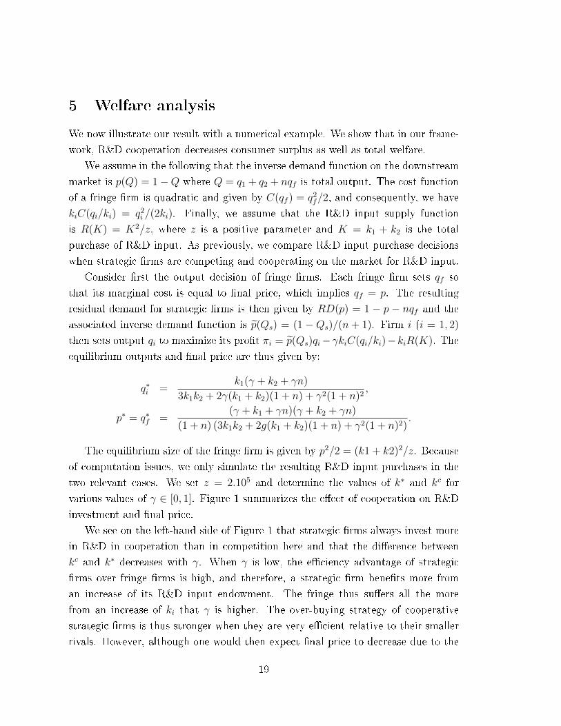
5 Welfare analysis
We now illustrate our result with a numerical example. We show that in our frame-
work, R&D cooperation decreases consumer surplus as well as total welfare.
We assume in the following that the inverse demand function on the downstream
market is p(Q) = 1−Q where Q = q1 + q2 + nqf is total output. The cost function
of a fringe �rm is quadratic and given by C(qf ) = q2f/2, and consequently, we have
kiC(qi/ki) = q2i /(2ki). Finally, we assume that the R&D input supply function
is R(K) = K2/z, where z is a positive parameter and K = k1 + k2 is the total
purchase of R&D input. As previously, we compare R&D input purchase decisions
when strategic �rms are competing and cooperating on the market for R&D input.
Consider �rst the output decision of fringe �rms. Each fringe �rm sets qf so
that its marginal cost is equal to �nal price, which implies qf = p. The resulting
residual demand for strategic �rms is then given by RD(p) = 1 − p − nqf and the
associated inverse demand function is p̃(Qs) = (1−Qs)/(n+ 1). Firm i (i = 1, 2)
then sets output qi to maximize its pro�t πi = p̃(Qs)qi−γkiC(qi/ki)−kiR(K). The
equilibrium outputs and �nal price are thus given by:
q∗i =k1(γ + k2 + γn)
3k1k2 + 2γ(k1 + k2)(1 + n) + γ2(1 + n)2,
p∗ = q∗f =(γ + k1 + γn)(γ + k2 + γn)
(1 + n) (3k1k2 + 2g(k1 + k2)(1 + n) + γ2(1 + n)2).
The equilibrium size of the fringe �rm is given by p2/2 = (k1 + k2)2/z. Because
of computation issues, we only simulate the resulting R&D input purchases in the
two relevant cases. We set z = 2.105 and determine the values of k∗ and kc for
various values of γ ∈ [0, 1]. Figure 1 summarizes the e�ect of cooperation on R&D
investment and �nal price.
We see on the left-hand side of Figure 1 that strategic �rms always invest more
in R&D in cooperation than in competition here and that the di�erence between
kc and k∗ decreases with γ. When γ is low, the e�ciency advantage of strategic
�rms over fringe �rms is high, and therefore, a strategic �rm bene�ts more from
an increase of its R&D input endowment. The fringe thus su�ers all the more
from an increase of ki that γ is higher. The over-buying strategy of cooperative
strategic �rms is thus stronger when they are very e�cient relative to their smaller
rivals. However, although one would then expect �nal price to decrease due to the
19

Figure 1: R&D investment (left-hand) and �nal price (right-hand) with respect tostrategic �rms cost advantage γ, with competition (full line) and cooperation (dottedline).
enhancing of global e�ciency, this never happens, as is predicted by Proposition
1: the cooperative �nal price is also higher than the competitive �nal price for all
γ ∈ [0, 1). Consumer surplus here is simply given by SC = (1− p)2/2, from which we
deduce that consumer surplus is always lower when strategic �rms cooperate in R&D
than when they compete in R&D. Total welfare is then given by W = π∗1 +π∗2 +SC.
As Figure 2 shows, welfare is lower with R&D cooperation than competition for all
values of γ.
The inverted U-shape of R&D purchase, and consequently of �nal prices, comes
from two di�erent e�ects. When γ is close to 1, the cost advantage of a strategic
�rm over the fringe is very low. Then, an increase of i's R&D purchase does not
increase its cost advantage so much. This explains why as γ decreases, strategic
�rms increase their R&D purchases in competition as well as in cooperation. By
contrast, when γ is close to 0, the cost advantage of a strategic �rm is already so
high that strategic �rms sell most of the output. Then, an increase of i's R&D
purchase, while highly increasing its cost advantage, cannot lead to a very high
output increase and hence does not bene�t the strategic �rm. This explains why
R&D input purchase decreases as γ tends to 0.
6 Extensions
In this section, using the framework speci�ed in Section 5, we show that our result
is robust to some extent to allowing the R&D cost to also depend on fringe �rms'
20
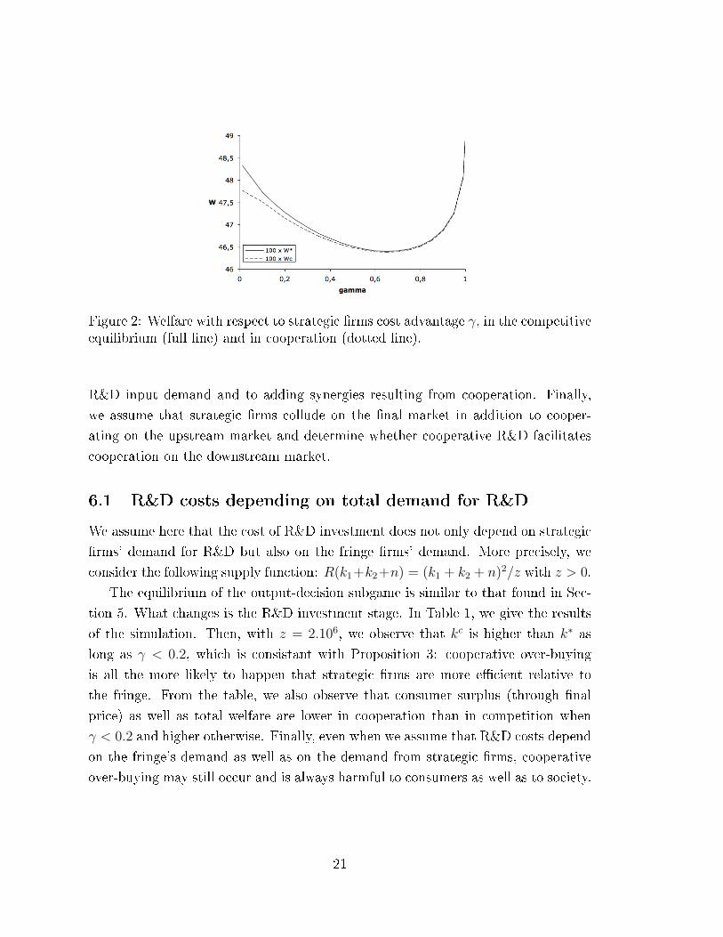
Figure 2: Welfare with respect to strategic �rms cost advantage γ, in the competitiveequilibrium (full line) and in cooperation (dotted line).
R&D input demand and to adding synergies resulting from cooperation. Finally,
we assume that strategic �rms collude on the �nal market in addition to cooper-
ating on the upstream market and determine whether cooperative R&D facilitates
cooperation on the downstream market.
6.1 R&D costs depending on total demand for R&D
We assume here that the cost of R&D investment does not only depend on strategic
�rms' demand for R&D but also on the fringe �rms' demand. More precisely, we
consider the following supply function: R(k1+k2+n) = (k1 + k2 + n)2/z with z > 0.
The equilibrium of the output-decision subgame is similar to that found in Sec-
tion 5. What changes is the R&D investment stage. In Table 1, we give the results
of the simulation. Then, with z = 2.106, we observe that kc is higher than k∗ as
long as γ < 0.2, which is consistant with Proposition 3: cooperative over-buying
is all the more likely to happen that strategic �rms are more e�cient relative to
the fringe. From the table, we also observe that consumer surplus (through �nal
price) as well as total welfare are lower in cooperation than in competition when
γ < 0.2 and higher otherwise. Finally, even when we assume that R&D costs depend
on the fringe's demand as well as on the demand from strategic �rms, cooperative
over-buying may still occur and is always harmful to consumers as well as to society.
21
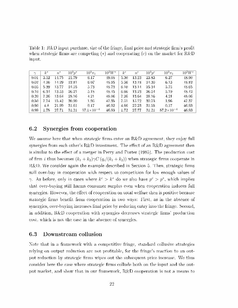
Table 1: R&D input purchase, size of the fringe, �nal price and strategic �rm's pro�twhen strategic �rms are competing (∗) and cooperating (c) on the market for R&Dinput.
γ k∗ n∗ 103p∗ 103π1 102W ∗ kc nc 103pc 103π1 102W c
0.01 3.52 14.75 21.79 6.17 49.08 5.30 13.23 23.83 6.27 48.900.02 4.26 14.29 22.81 6.07 48.95 5.56 13.18 24.30 6.13 48.820.05 5.39 13.77 24.55 5.73 48.72 6.10 13.14 25.34 5.75 48.650.10 6.34 13.53 26.21 5.18 48.45 6.66 13.23 26.54 5.19 48.420.20 7.26 13.64 28.16 4.21 48.06 7.26 13.64 28.16 4.21 48.060.50 7.74 15.42 30.90 1.95 47.35 7.51 15.72 30.73 1.96 47.370.90 4.8 21.99 31.61 0.17 46.92 4.66 22.23 31.55 0.17 46.930.99 1.75 27.71 31.21 57.1×10⁻⁴ 46.93 1.72 27.77 31.21 57.2×10⁻⁴ 46.93
6.2 Synergies from cooperation
We assume here that when strategic �rms enter an R&D agreement, they enjoy full
synergies from each other's R&D investment. The e�ect of an R&D agreement then
is similar to the e�ect of a merger in Perry and Porter (1985). The production cost
of �rm i thus becomes (k1 + k2)γC (qi/(k1 + k2)) when strategic �rms cooperate in
R&D. We consider again the example described in Section 5. Then, strategic �rms
still over-buy in cooperation with respect to competition for low enough values of
γ. As before, only in cases where kc > k∗ do we also have pc > p∗, which implies
that over-buying still harms consumer surplus even when cooperation induces full
synergies. However, the e�ect of cooperation on total welfare then is positive because
strategic �rms bene�t from cooperation in two ways: First, as in the absence of
synergies, over-buying increases �nal price by reducing entry into the fringe. Second,
in addition, R&D cooperation with synergies decreases strategic �rms' production
cost, which is not the case in the absence of synergies.
6.3 Downstream collusion
Note that in a framework with a competitive fringe, standard collusive strategies
relying on output reduction are not pro�table, for the fringe's reaction to an out-
put reduction by strategic �rms wipes out the subsequent price increase. We thus
consider here the case where strategic �rms collude both on the input and the out-
put market, and show that in our framework, R&D cooperation is not a means to
22

facilitate collusion on the �nal market.
For simplicity, consider again the speci�c framework described in the Section 5.
Assume that strategic �rms now maximize the joint pro�t of the strategic duopoly
both on the R&D input market and on the �nal market, i.e. enforce collusion on
the �nal market.
Output decisions of the fringe �rms are again given by p = qf and the residual
inverse demand function is still p̃(Qs). Then, �rm i sets output qi to maximize pro�t
πi + πj = p̃(Qs)Qs − γ(kiC( qiki ) + kjC(qjkj)) − (ki + kj)R(K). The collusive outputs
and �nal price are thus given by:
qMi =ki
γ(n+ 1) + 2(k1 + k2),
pM =γ(n+ 1) + k1 + k2
(n+ 1)(γ(n+ 1) + 2(k1 + k2).
Unsurprisingly, for a given size of the fringe, the resulting �nal price (and hence the
output of a fringe �rm) is higher than in the competitive equilibrium. Besides, if
strategic �rms both buy the same amount of R&D input, �rm i's output is reduced
in collusion as compared to competition. The direct consequence however is that
more �rms enter the fringe than in the competitive case: nM(k, k) > n∗(k, k) for any
k > 1, which reduces the �nal price as well as the output of strategic �rms. Then,
if the di�erence between nM and n∗ is high enough, the pro�t of strategic �rm is
higher in competition than in collusion for any value of k.
For z = 2.106, it is always the case that the pro�t of a strategic �rm in com-
petition is higher than its pro�t in collusion: π∗i (k, k) > πMi (k, k). In particular,
since π∗i (kc, kc) > π∗i (k, k) for all k > 1, we always have π∗i (k
c, kc) > πMi (k, k). In
other words, it is impossible for strategic �rms to earn a higher pro�t when they
enforce collusion successively on the market for R&D input and on the �nal market
than when they only cooperate on the market for R&D input. Indeed, collusion
on the �nal market increases the �nal price and therefore facilitates entry in the
competitive fringe. Eventually, the increased competition on the �nal market more
than o�sets the initial price increase.
The usual concerns regarding the potential anti-competitive e�ects of R&D
agreements are that cooperation at any stage of the production process (here, R&D)
can facilitate cooperation in other stages, and in particular at the pricing stage. In-
23

terestingly enough, in our case, collusion on the �nal market would not be pro�table
for strategic �rms. More importantly, the anti-competitive e�ect of R&D we observe
thus does not result from softer competition between strategic �rms on the �nal mar-
ket: It results from softer competition between strategic �rms and the competitive
fringe, which has been analyzed in the previous Sections.
7 Conclusion
In this paper, we highlight an anti-competitive e�ect of R&D agreements that has
not been pointed out in the previous literature. In order to engage in R&D, �rms
must purchase speci�c inputs including high skilled workers or time slots for the use
of a rare facility. Such inputs are necessary to all the �rms engaging in the same
type of research. Consequently, �rms that compete to sell a �nal good are also likely
to compete to purchase the inputs necessary to R&D.
We show that in such situations, if there are large size or cost asymmetries
between �rms on the market, as can be the case in industries such as software
designing or pharmaceutical R&D, large �rms with market power may engage in
R&D cooperation for anti-competitive purposes. Cooperation may then induce them
to overbuy the input, i.e. to buy more input than they would otherwise, so as to
increase the input price or make it less available to small �rms, and thus to exclude
them from the �nal market. This strategy is all the more likely to occur that
large �rms are very e�cient relative to their small rivals. In such a context, while
one would expect �nal prices to decrease due to enhanced e�ciency, the market
concentration e�ect induces an increase in the �nal price. Such agreements thus
harm consumer surplus.
A Appendix
A.1 Strategic substitutes
We show here that when the size of the fringe n is �xed, the output decisions of
the strategic �rms are strategic substitutes. Deriving equation (3) with respect to
24
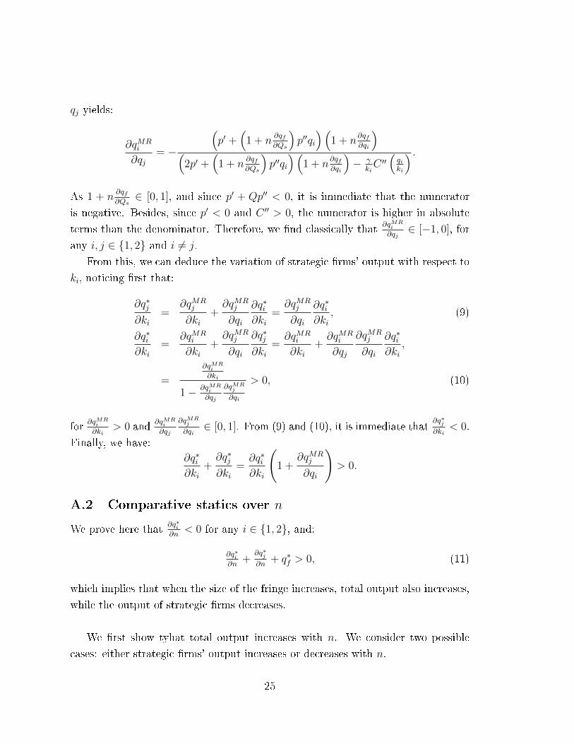
qj yields:
∂qMRi
∂qj= −
(p′ +
(1 + n
∂qf∂Qs
)p′′qi
)(1 + n
∂qf∂qi
)(2p′ +
(1 + n
∂qf∂Qs
)p′′qi
)(1 + n
∂qf∂qi
)− γ
kiC ′′(qiki
) .As 1 + n
∂qf∂Qs∈ [0, 1], and since p′ + Qp′′ < 0, it is immediate that the numerator
is negative. Besides, since p′ < 0 and C ′′ > 0, the numerator is higher in absolute
terms than the denominator. Therefore, we �nd classically that∂qMR
i
∂qj∈ [−1, 0], for
any i, j ∈ {1, 2} and i 6= j.
From this, we can deduce the variation of strategic �rms' output with respect to
ki, noticing �rst that:
∂q∗j∂ki
=∂qMR
j
∂ki+∂qMR
j
∂qi
∂q∗i∂ki
=∂qMR
j
∂qi
∂q∗i∂ki
, (9)
∂q∗i∂ki
=∂qMR
i
∂ki+∂qMR
j
∂qi
∂q∗j∂ki
=∂qMR
i
∂ki+∂qMR
i
∂qj
∂qMRj
∂qi
∂q∗i∂ki
,
=
∂qMRi
∂ki
1− ∂qMRi
∂qj
∂qMRj
∂qi
> 0, (10)
for∂qMR
i
∂ki> 0 and
∂qMRi
∂qj
∂qMRj
∂qi∈ [0, 1]. From (9) and (10), it is immediate that
∂q∗j∂ki
< 0.
Finally, we have:
∂q∗i∂ki
+∂q∗j∂ki
=∂q∗i∂ki
(1 +
∂qMRj
∂qi
)> 0.
A.2 Comparative statics over n
We prove here that∂q∗i∂n
< 0 for any i ∈ {1, 2}, and:
∂q∗i∂n
+∂q∗j∂n
+ q∗f > 0, (11)
which implies that when the size of the fringe increases, total output also increases,
while the output of strategic �rms decreases.
We �rst show tyhat total output increases with n. We consider two possible
cases: either strategic �rms' output increases or decreases with n.
25

Assume �rst that we have∂q∗1∂n
+∂q∗2∂n
> 0. Then it is immediate that (11) is
satis�ed. Assume now that on the contrary we have∂q∗1∂n
+∂q∗2∂n
< 0. Then there
exists i such that∂q∗i∂n
< 0. Consider the derivative of ∂πi∂qi
with respect to n and have
the following equation:
∂2πi∂qi∂n
=
(∂qi∗∂n
+∂q∗j∂n
+ q∗f
)[(1 + n
∂qf∂qi
)(p′ +
(1 + n
∂qf∂qi
)p′′q∗i
)+ nq∗i p
′∂2qf∂q2i
]+
(1 + n
∂qf∂qi
)(∂qf∂qi
q∗i +∂q∗i∂n
)p′ − γ
ki
∂q∗i∂n
C ′′(q∗iki
)= 0, (12)
since for any value of n, we always have that ∂πi∂qi
(q∗i , q∗j , q∗f ) = 0. Besides, we know
that C ′′ > 0, p′ < 0 and and∂qf∂qi
< 0. As we also have∂q∗i∂n
< 0, we can write
that(1 + n
∂qf∂qi
)(∂qf∂qiq∗i +
∂q∗i∂n
)p′− γ
ki
∂q∗i∂nC ′′(q∗iki
)> 0, and consequently, we have the
following inequality:(∂q∗i∂n
+∂q∗j∂n
+ q∗f
)[(1 + n
∂qf∂qi
)(p′ +
(1 + n
∂qf∂qi
)p′′q∗i
)+ nq∗i p
′∂2qf∂q2i
]< 0.
(13)
Therefore, if we �nd that the right term of this product is always negative, then it
immediately follows that∂q∗i∂n
+∂q∗j∂n
+ q∗f > 0. In order to show that this is true, we
now di�erentiate ∂πi∂qi
with respect to kj. Using the same reasoning, we �nd:
∂2πi∂qi∂kj
=
(∂q∗i∂kj
+∂q∗j∂kj
)[(1 + n
∂qf∂qi
)(p′ +
(1 + n
∂qf∂qi
)p′′q∗i
)+ nq∗i p
′∂2qf∂q2i
]+
(1 + n
∂qf∂qi
)∂q∗i∂kj
p′ − 1
ki
∂q∗i∂kj
C ′′(q∗iki
)= 0. (14)
Since p′ < 0, C ′′ > 0 and∂q∗i∂kj
< 0, we have the following inequality:
(∂q∗i∂kj
+∂q∗j∂kj
)[(1 + n
∂qf∂qi
)(p′ +
(1 + n
∂qf∂qi
)p′′q∗i
)+ nq∗i p
′∂2qf∂q2i
]< 0.
Besides, we know that∂q∗i∂kj
+∂q∗j∂kj
> 0: the output of strategic �rms increases when
one of the strategic �rm increases its R&D input purchase. It thus follows that:(1 + n
∂qf∂qi
)(p′ +
(1 + n
∂qf∂qi
)p′′q∗i
)+ nq∗i p
′∂2qf∂q2i
< 0. (15)
26
From this and (13), we deduce that (11) is satis�ed.
We now show by contradiction that we always have∂q∗i∂n≤ 0: the output of
strategic �rm i decreases with n. Assume that there exists i such that∂q∗i∂n
> 0. This
implies that:(1 + n
∂qf∂qi
)∂qf∂qi
q∗i +∂q∗i∂n
((1 + n
∂qf∂qi
)p′ − γ
kiC ′′(q∗iki
))< 0.
Then it follows from (12) and (15) that∂q∗i∂n
+∂q∗j∂n
+ q∗f < 0, which as we have shown
is not true. Finally, we always have∂q∗i∂n≤ 0, and therefore
∂q∗i∂n
+∂q∗j∂n
+ q∗f ∈ [0, q∗f ].
A.3 Proof of Proposition 2
We show here that the output of strategic �rm j may increase with its strategic
rival's R&D investment. The variation of q∗∗j with respect to ki is given by:
∂q∗∗j∂ki
=∂q∗j∂ki
+∂q∗j∂n
∂n∗
∂ki.
In order to simplify expressions, we use the following notations:
A =∂q∗i∂n
+∂q∗j∂n
+q∗∗f , B =∂q∗i∂kj
+∂q∗j∂kj
, X = 1+n∂qf∂Qs
, T = X(p′+Xp′′qi)+nqip′∂
2qf∂Q2
s
.
Equations (7), (12) and (14) yield:
∂q∗∗j∂ki
= − BT
Xp′ − γkjC ′′(q∗∗jkj
) − R′ −BXq∗∗f p′
AXq∗∗f p′
AT +X∂qf∂Qs
q∗∗j
Xp′ − γkjC ′′(q∗∗jkj
) ,= −
R′(AT +X
∂qf∂Qs
qi
)−BX2q∗∗f q
∗∗j p′ ∂qf∂Qs
AXq∗∗f p′(Xp′ − γ
kjC ′′(q∗∗jkj
))
27

SinceXp′− γkjC ′′(q∗∗jkj
)< 0,
∂q∗∗j∂ki
is of the sign of−R′(AT +X
∂qf∂Qs
qi
)+BX2qfqip
′ ∂qf∂Qs
,
and is thus positive as long as:
∂2qf∂Q2
s
>1
nq∗∗j p′
(∂qf∂Qs
BX2q∗∗f q∗∗j p′ −R′Xq∗∗j
R′A−X(p′ +Xp′′q∗∗j )
).
Besides, from (2) we �nd that:
∂2qf∂Q2
s
=
(∂qf∂Qs
)2p′′(Q)C ′′(qf )
2 − C ′′′(qf )p′(Q)2
p′(Q)2.
Therefore, the condition for∂q∗∗j∂ki
to be positive is:
p′′(Q∗∗)C ′′(q∗∗f )2−C ′′′(q∗∗f )p′(Q∗∗)2 >p′(Q∗∗)
nq∗∗j∂qf∂Qs
(BX2q∗∗f q
∗∗j p′ −R′Xq∗∗j
R′A−X(p′(Q∗∗) +Xp′′(Q∗∗)q∗∗j )
∂qf∂Qs
).
The right-hand side of the latter inequality is negative. In particular, if p′′(Q)C ′′(qf )2−
C ′′′(qf )p′(Q)2 > 0, then it is true
∂q∗∗j∂ki
> 0.
A.4 Proof of Lemma 2
Consider �rst the second stage of the game, which corresponds to Stage 2 in the
main framework. Each �rm i (i = 1, 2) sets its output qi in order to maximize its
individual pro�t, and thus solves the problem: maxqi πi = p(Qs)qi − kiR(k1 + k2),
and the �rst order conditions are thus given by:
p+ qip′ = γC ′
(qiki
). (16)
Following the same reasoning as in the previous section, we �nd that ∂q∗i /∂ki > 0,
∂q∗j/∂ki < 0 and ∂q∗i /∂ki + ∂q∗j/∂ki > 0.
In the �rst stage of the game, the di�erence between cooperation and competition
is given by:
∂πj∂ki
(q∗1, q∗2) = p′q∗j
∂q∗i∂ki
+∂q∗j∂ki
(p+ p′q∗j − γC ′
(q∗jkj
))− kjR′.
We can simplify this expression using (16) and �nd that ∂πj/∂ki = p′q∗j∂q∗i /∂ki −
28

kjR′. As p′ < 0 and R′ > 0, it is immediate that it is negative for all values of ki
and kj, hence Lemma 2.
A.5 Proof of Lemma 3
When the cost of a �rm only depends on its own R&D investment, equation (5) be-
comes simply p∗q∗f−C(q∗f ) = R, and equation (6) becomes (∂p∗/∂ki + ∂p∗/∂n∂n∗/∂ki) q∗f =
0, as neither the increase of ki nor the entry of a new fringe �rm raises the price of
the R&D input. Given that q∗f > 0, the e�ect of an increase of R&D input purchase
on the size of the fringe is simply:
∂n∗
∂ki= −
∂p∗
∂ki∂p∗
∂n
= −∂q∗i∂ki
+∂q∗j∂ki
∂q∗i∂n
+∂q∗j∂n
+ q∗∗f
. (17)
Obviously, it is still negative as the short-term pro�t of fringe �rms is still reduced
following an increase of ki. However, since q∗∗f > 0, it is straightforward that we now
have ∂p∗∗/∂ki = 0.
References
[1] D.W. Carlton and S.C. Salop. You keep on knocking but you can't come in:
Evaluating restrictions on access to input joint ventures. Harvard Journal of
Law & Technology, 9(2):319 � 352, 1996.
[2] Z. Chen and T.W. Ross. Strategic alliances, shared facilities, and entry deter-
rence. The RAND Journal of Economics, 31(2):pp. 326�344, 2000.
[3] Z. Chen and T.W. Ross. Cooperating upstream while competing downstream: a
theory of input joint ventures. International Journal of Industrial Organization,
21(3):381 � 397, 2003.
[4] European Commission. Guidelines on the applicability of Article 101 of the
EC Treaty on the Functioning of the European Union to horizontal coopera-
tion agreements. O�cial Journal of the European Union, 2011/C:11/01�11/72,
2011.
29
[5] R.W. Cooper and T.W. Ross. Sustaining Cooperation with Joint Ventures.
Journal of Law, Economics, and Organization, 25(1):31�54, 2009.
[6] C. D'Aspremont and A. Jacquemin. Cooperative and noncooperative R&D in
duopoly with spillovers. The American Economic Review, 78(5):pp. 1133�1137,
1988.
[7] GM Grossman and C. Shapiro. Research joint ventures: an antitrust analysis.
Journal of Law, Economics, and Organization, 2(2):315�337, 1986.
[8] M.I. Kamien, E. Muller, and I. Zang. Research joint ventures and R&D cartels.
The American Economic Review, 82(5):pp. 1293�1306, 1992.
[9] W.J. Nuttall. Nuclear renaissance: technologies and policies for the future of
nuclear power. IOP, 2005.
[10] Martin K Perry and Robert H Porter. Oligopoly and the incentive for horizontal
merger. The American Economic Review, 75(1):219�227, 1985.
[11] M. Riordan. Anticompetitive vertical integration by a dominant �rm. American
Economic Review, 88(5):1232�1248, 1998.
[12] S. Salop and D. Sche�man. Raising rivals costs. American Economic Review,
73(2):267�271, 1983.
[13] S. Salop and D. Sche�man. Cost-raising strategies. The Journal of Industrial
Economics, 36(1):19�34, 1987.
[14] R.D. Simpson and N.S. Vonortas. Cournot equilibrium with imperfectly appro-
priable R&D. The Journal of Industrial Economics, 42(1):79�92, 1994.
[15] SS Yi. Endogenous formation of joint ventures with e�ciency gains. The RAND
Journal of Economics, 29(3):610�631, 1998.
30
PREVIOUS DISCUSSION PAPERS
38 Christin, Clémence, Entry Deterrence Through Cooperative R&D Over-Investment, November 2011.
37 Haucap, Justus, Herr, Annika and Frank, Björn, In Vino Veritas: Theory and Evidence on Social Drinking, November 2011.
36 Barth, Anne-Kathrin and Graf, Julia, Irrationality Rings! – Experimental Evidence on Mobile Tariff Choices, November 2011.
35 Jeitschko, Thomas D. and Normann, Hans-Theo, Signaling in Deterministic and Stochastic Settings, November 2011.
34 Christin, Cémence, Nicolai, Jean-Philippe and Pouyet, Jerome, The Role of Abatement Technologies for Allocating Free Allowances, October 2011.
33 Keser, Claudia, Suleymanova, Irina and Wey, Christian, Technology Adoption in Markets with Network Effects: Theory and Experimental Evidence, October 2011.
32 Catik, A. Nazif and Karaçuka, Mehmet, The Bank Lending Channel in Turkey: Has it Changed after the Low Inflation Regime?, September 2011. Forthcoming in: Applied Economics Letters.
31 Hauck, Achim, Neyer, Ulrike and Vieten, Thomas, Reestablishing Stability and Avoiding a Credit Crunch: Comparing Different Bad Bank Schemes, August 2011.
30 Suleymanova, Irina and Wey, Christian, Bertrand Competition in Markets with Network Effects and Switching Costs, August 2011. Published in: B.E. Journal of Economic Analysis & Policy, 11 (2011), Article 56.
29 Stühmeier, Torben, Access Regulation with Asymmetric Termination Costs, July 2011.
28 Dewenter, Ralf, Haucap, Justus and Wenzel, Tobias, On File Sharing with Indirect Network Effects Between Concert Ticket Sales and Music Recordings, July 2011.
27 Von Schlippenbach, Vanessa and Wey, Christian, One-Stop Shopping Behavior, Buyer Power, and Upstream Merger Incentives, June 2011.
26 Balsmeier, Benjamin, Buchwald, Achim and Peters, Heiko, Outside Board Memberships of CEOs: Expertise or Entrenchment?, June 2011.
25 Clougherty, Joseph A. and Duso, Tomaso, Using Rival Effects to Identify Synergies and Improve Merger Typologies, June 2011. Published in: Strategic Organization, 9 (2011), pp. 310-335.
24 Heinz, Matthias, Juranek, Steffen and Rau, Holger A., Do Women Behave More Reciprocally than Men? Gender Differences in Real Effort Dictator Games, June 2011. Forthcoming in: Journal of Economic Behavior and Organization.
23 Sapi, Geza and Suleymanova, Irina, Technology Licensing by Advertising Supported Media Platforms: An Application to Internet Search Engines, June 2011. Published in: B. E. Journal of Economic Analysis & Policy, 11 (2011), Article 37.

22 Buccirossi, Paolo, Ciari, Lorenzo, Duso, Tomaso, Spagnolo Giancarlo and Vitale, Cristiana, Competition Policy and Productivity Growth: An Empirical Assessment, May 2011.
21 Karaçuka, Mehmet and Catik, A. Nazif, A Spatial Approach to Measure Productivity Spillovers of Foreign Affiliated Firms in Turkish Manufacturing Industries, May 2011. Forthcoming in: The Journal of Developing Areas.
20 Catik, A. Nazif and Karaçuka, Mehmet, A Comparative Analysis of Alternative Univariate Time Series Models in Forecasting Turkish Inflation, May 2011. Forthcoming in: Journal of Business Economics and Management.
19 Normann, Hans-Theo and Wallace, Brian, The Impact of the Termination Rule on Cooperation in a Prisoner’s Dilemma Experiment, May 2011. Forthcoming in: International Journal of Game Theory.
18 Baake, Pio and von Schlippenbach, Vanessa, Distortions in Vertical Relations, April 2011. Published in: Journal of Economics, 103 (2011), pp. 149-169.
17 Haucap, Justus and Schwalbe, Ulrich, Economic Principles of State Aid Control, April 2011. Forthcoming in: F. Montag & F. J. Säcker (eds.), European State Aid Law: Article by Article Commentary, Beck: München 2012.
16 Haucap, Justus and Heimeshoff, Ulrich, Consumer Behavior towards On-net/Off-net Price Differentiation, January 2011. Published in: Telecommunication Policy, 35 (2011), pp. 325-332.
15 Duso, Tomaso, Gugler, Klaus, Yurtoglu, Burcin B., How Effective is European Merger Control? January 2011. Published in: European Economic Review, 55 (2011), pp. 980‐1006.
14 Haigner, Stefan D., Jenewein, Stefan, Müller, Hans Christian and Wakolbinger, Florian, The First shall be Last: Serial Position Effects in the Case Contestants evaluate Each Other, December 2010. Published in: Economics Bulletin, 30 (2010), pp. 3170-3176.
13 Suleymanova, Irina and Wey, Christian, On the Role of Consumer Expectations in Markets with Network Effects, November 2010 (first version July 2010). Forthcoming in: Journal of Economics.
12 Haucap, Justus, Heimeshoff, Ulrich and Karaçuka, Mehmet, Competition in the Turkish Mobile Telecommunications Market: Price Elasticities and Network Substitution, November 2010. Published in: Telecommunications Policy, 35 (2011), pp. 202-210.
11 Dewenter, Ralf, Haucap, Justus and Wenzel, Tobias, Semi-Collusion in Media Markets, November 2010. Published in: International Review of Law and Economics, 31 (2011), pp. 92-98.
10 Dewenter, Ralf and Kruse, Jörn, Calling Party Pays or Receiving Party Pays? The Diffusion of Mobile Telephony with Endogenous Regulation, October 2010. Published in: Information Economics and Policy, 23 (2011), pp. 107-117.
09 Hauck, Achim and Neyer, Ulrike, The Euro Area Interbank Market and the Liquidity Management of the Eurosystem in the Financial Crisis, September 2010.

08 Haucap, Justus, Heimeshoff, Ulrich and Luis Manuel Schultz, Legal and Illegal Cartels in Germany between 1958 and 2004, September 2010. Published in: H. J. Ramser & M. Stadler (eds.), Marktmacht. Wirtschaftswissenschaftliches Seminar Ottobeuren, Volume 39, Mohr Siebeck: Tübingen 2010, pp. 71-94.
07 Herr, Annika, Quality and Welfare in a Mixed Duopoly with Regulated Prices: The Case of a Public and a Private Hospital, September 2010. Published in: German Economic Review, 12 (2011), pp. 422-437.
06 Blanco, Mariana, Engelmann, Dirk and Normann, Hans-Theo, A Within-Subject Analysis of Other-Regarding Preferences, September 2010. Published in: Games and Economic Behavior, 72 (2011), pp. 321-338.
05 Normann, Hans-Theo, Vertical Mergers, Foreclosure and Raising Rivals’ Costs – Experimental Evidence, September 2010. Published in: The Journal of Industrial Economics, 59 (2011), pp. 506-527.
04 Gu, Yiquan and Wenzel, Tobias, Transparency, Price-Dependent Demand and Product Variety, September 2010. Published in: Economics Letters, 110 (2011), pp. 216-219.
03 Wenzel, Tobias, Deregulation of Shopping Hours: The Impact on Independent Retailers and Chain Stores, September 2010. Published in: Scandinavian Journal of Economics, 113 (2011), pp. 145-166.
02 Stühmeier, Torben and Wenzel, Tobias, Getting Beer During Commercials: Adverse Effects of Ad-Avoidance, September 2010. Published in: Information Economics and Policy, 23 (2011), pp. 98-106.
01 Inderst, Roman and Wey, Christian, Countervailing Power and Dynamic Efficiency, September 2010. Published in: Journal of the European Economic Association, 9 (2011), pp. 702-720.

ISSN 2190-9938 (online) ISBN 978-3-86304-037-6


