Environmental & Engineering Geoscience

Environmental &Engineering GeoscienceMAY 2015 VOLUME XXI, NUMBER 2

THE JOINT PUBLICATION OF THE

ASSOCIATION OF ENVIRONMENTAL AND ENGINEERING GEOLOGISTS

AND THE GEOLOGICAL SOCIETY OF AMERICA

SERVING PROFESSIONALS IN

ENGINEERING GEOLOGY, ENVIRONMENTAL GEOLOGY, AND HYDROGEOLOGY

Environmental & Engineering Geoscience (ISSN 1078-7275) is pub-lished quarterly by the Association of Environmental and EngineeringGeologists (AEG) and the Geological Society of America (GSA).Periodicals postage paid at AEG, 1100 Brandywine Blvd, Suite H,Zanesville, OH 43701-7301. Phone: 844-331-7867 and additional mail-ing offices.

EDITORIAL OFFICE: Environmental & EngineeringGeoscience journal, Department of Geology, Kent StateUniversity, Kent, OH 44242, U.S.A. phone: 330-672-2968, fax:330-672-7949, [email protected].

CLAIMS: Claims for damaged or not received issues will behonored for 6 months from date of publication. AEG membersshould contact AEG, 1100 Brandywine Blvd, Suite H, Zanesville, OH43701-7301. Phone: 844-331-7867. GSA members who are notmembers of AEG should contact the GSA Member Service cen-ter. All claims must be submitted in writing.

POSTMASTER: Send address changes to AEG, 1100Brandywine Blvd, Suite H, Zanesville, OH 43701-7301. Phone: 844-331-7867. Include both old and new addresses, with ZIP code.Canada agreement number PM40063731. Return undeliverableCanadian addresses to Station A P.O. Box 54, Windsor, ON N9A6J5 Email: [email protected].

DISCLAIMER NOTICE: Authors alone are responsible forviews expressed in articles. Advertisers and their agencies aresolely responsible for the content of all advertisements printed andalso assume responsibility for any claims arising therefromagainst the publisher. AEG and Environmental & EngineeringGeoscience reserve the right to reject any advertising copy.

SUBSCRIPTIONS:

Member subscriptions: AEG members automatically receive the journal as part of their AEG membership dues. Additionalsubscriptions may be ordered at $40 per year. GSA memberswho are not members of AEG may order for $40 per year ontheir annual GSA dues statement or by contacting GSA.

Nonmember subscriptions are $175 and may be ordered fromthe subscription department of either organization. A postagedifferential of $10 may apply to nonmember subscribers outsidethe United States, Canada, and Pan America. Contact AEG at303-757-2926; contact GSA Subscription Services, c/oAmerican Institute of Physics, 2 Huntington Quadrangle, Suite1N01, Melville, NY 11747-4502.

Single copies are $50.00 each. Requests for single copies shouldbe sent to AEG, 1100 Brandywine Blvd, Suite H, Zanesville, OH43701-7301. Phone: 844-331-7867.

© 2015 by the Association of Environmental and EngineeringGeologists

All rights reserved. No part of this publication may be reproduced or transmitted in any form or by any means, electronic or mechanical, including photocopying, recording, orby any information storage and retrieval system, without permission in writing from AEG.

THIS PUBLICATION IS PRINTED ON ACID-FREE PAPER

ABDUL SHAKOORDepartment of GeologyKent State University

Kent, OH 44242330-672-2968

[email protected]

BRIAN G. KATZFlorida Department of Environmental

Protection2600 Blair Stone Rd.Tallahassee, FL 32399

[email protected]

EDITORSCover photo

Coastal bluff landslide in Quaternary glacial drift in the Dungeness littoral cell,Strait of Juan de Fuca near Port Angeles, Washington, USA. Photo Credit: DavidParks; see related article on pp. 129 to 146.

SUBMISSION OF MANUSCRIPTS

Environmental & Engineering Geoscience (E&EG), is a quar-terly journal devoted to the publication of original papers thatare of potential interest to hydrogeologists, environmental andengineering geologists, and geological engineers working in siteselection, feasibility studies, investigations, design or construc-tion of civil engineering projects or in waste management,groundwater, and related environmental fields. All papers arepeer reviewed.

The editors invite contributions concerning all aspects of envi-ronmental and engineering geology and related disciplines.Recent abstracts can be viewed under “Archive” at the website, “http://eeg.geoscienceworld.org”. Articles that report onresearch, case histories and new methods, and book reviewsare welcome. Discussion papers, which are critiques of print-ed articles and are technical in nature, may be published withreplies from the original author(s). Discussion papers andreplies should be concise.

To submit a manuscript go to http://eeg.allentrack.net. If youhave not used the system before, follow the link at the bottom ofthe page that says New users should register for an account.Choose your own login and password. Further instructions willbe available upon logging into the system. Please carefully readthe “Instructions for Authors”.

Authors do not pay any charge for color figures that are essen-tial to the manuscript. Manuscripts of fewer than 10 pages maybe published as Technical Notes.

For further information, you may contact Dr. Abdul Shakoor atthe editorial office.

JOHN W. BELL

Nevada Bureau of Mines andGeologyRICHARD E. JACKSON

(Book Reviews Editor)Geofirma Engineering, Ltd.JEFFREY R. KEATON

AMEC AmericasPAUL G. MARINOS

National Technical Universityof Athens, GreeceJUNE E. MIRECKI

U.S. Army Corps of EngineersPETER PEHME

Waterloo Geophysics, IncNICHOLAS PINTER

Southern Illinois University

PAUL M. SANTI

Colorado School of MinesROBERT L. SCHUSTER

U.S. Geological SurveyROY J. SHLEMON

R. J. Shlemon& Associates, Inc.GREG M. STOCK

National Park ServiceRESAT ULUSAY

Hacettepe University, TurkeyCHESTER F. “SKIP” WATTS

Radford UniversityTERRY R. WEST

Purdue University

EDITORIAL BOARD

ASSOCIATE EDITORS

JEROME V. DEGRAFF

USDA Forest ServiceTHOMAS J. BURBEY

Virginia Polytechnic InstituteSYED E. HASAN

University of Missouri, Kansas City

ROBERT H. SYDNOR

ConsulantCHESTER F. WATTS (SKIP)Radford University

Environmental &Engineering Geoscience

Volume 21, Number 2, May 2015

Table of Contents

75 Sources and Changes in Groundwater Quality with Increasing Urbanization, Northeastern Illinois

Hue-Hwa Hwang, Samuel V. Panno, and Keith C. Hackley

91 Sorption-Desorption Characteristics of Tetrabromobisphenol A on Humin and Sediment of Lake Chaohu,China

Suwen Yang, Shengrui Wang, Binghui Zheng, Fengchang Wu, and Qiang Fu

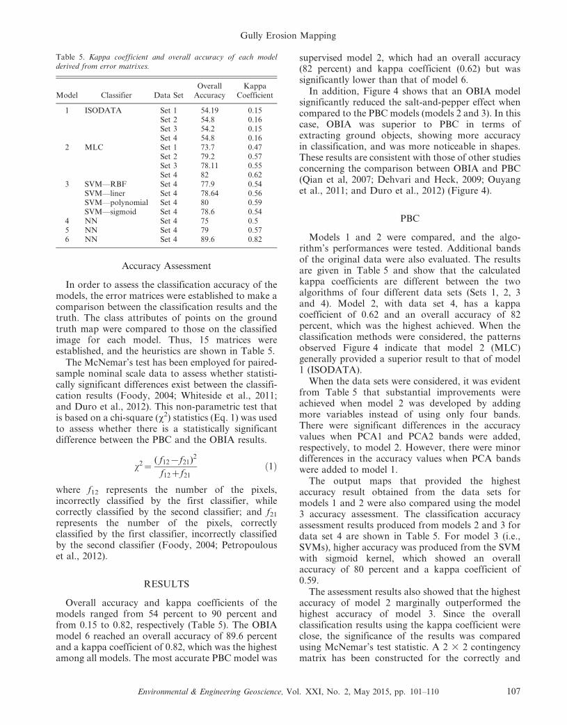
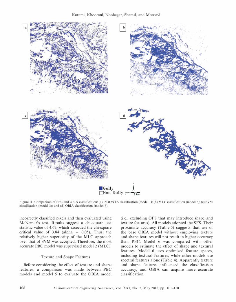
101 Gully Erosion Mapping Using Object-Based and Pixel-Based Image Classification Methods

Ayoob Karami, AsaDollah Khoorani, Ahmad Noohegar, Seyed Rashid Fallah Shamsi, and Vahid Moosavi

111 Near-Surface Geophysical Imaging of a Talus Deposit in Yosemite Valley, California

Anna G. Brody, Christopher J. Pluhar, Greg M. Stock, and W. Jason Greenwood

129 Bluff Recession in the Elwha and Dungeness Littoral Cells, Washington, USA

David S. Parks

147 Mine-Water Flow between Contiguous Flooded Underground Coal Mines with Hydraulically Compromised

Barriers

David D. M. Light and Joseph J. Donovan

Sources and Changes in Groundwater Quality with

Increasing Urbanization, Northeastern Illinois

HUE-HWA HWANG1

SAMUEL V. PANNO

KEITH C. HACKLEY2

Illinois State Geological Survey, Prairie Research Institute, University of Illinois,Champaign, IL 61820

Key Terms: Geochemistry, Environmental Geology,Pollution, Isotope Geochemistry, Agriculture

ABSTRACT

During the last decade of the twentieth century,McHenry County had the fastest-growing populationin Illinois. Just north of the Chicago metropolitanarea, land use in the eastern half of the county changedfrom row-crop agriculture to urban sprawl. Watersupplies are from shallow sand and gravel aquifers andare highly vulnerable. We evaluated the change ofgroundwater quality in McHenry County during mostof the twentieth century and identified the degree andextent of contamination, and sources, using availablehistoric water-quality data. To evaluate historic data,we calculated background concentrations of selectedions using cumulative probability plots to identifythe presence of anthropogenic contamination. Timingof groundwater contamination coincides with thatof population growth and the onset of utilization ofartificial N-fertilizer and road salt. Groundwater fromurban areas showed greater Na+ and Cl2 contents thanrural areas, which reflect more extensive applicationsof road salt beginning in the early 1960s. Groundwaterwas collected for chemical and isotope analyses fromselected shallow wells with historically elevated NO3

2

concentration as well as from farms with livestock.The isotope data suggest N-fertilizer and soil nitrogenare the predominant sources for NO3

2 in shallowgroundwater. Animal waste was also a source forNO3

2 near farms with livestock. Spatial analysissuggested that the source of NO3

2 in the groundwaterwas from surface-borne contaminants. The permeablesoils and near-surface sand and gravel aquifer found inmost of McHenry County provide pathways for

surface contaminants to migrate into shallow ground-water.

INTRODUCTION

The Chicago metropolitan area in northeasternIllinois recently has seen the most rapid increase inpopulation and land development in the state. Kelly(2008) found that the groundwater quality in theChicago metropolitan area has degraded since theearly 1900s, and the change appeared to have beenmost rapid in the outlying counties. McHenryCounty, located on the edge of the Chicago metro-politan area (Figure 1), has experienced the fastestgrowth rate of any county in Illinois between 1991and 2000 (U.S. Census Bureau, 2000). From 2001until 2010, McHenry County ranked seventh ingrowth rate of all Illinois counties (U.S. CensusBureau, 2010). Because of its rapid growth over thelast 20 years or so, and because its water supplies arealmost entirely from groundwater, McHenry Countyis an excellent region to study the anthropogenicimpacts on groundwater resources. The population ofMcHenry County increased from 35,000 in 1930 to183,000 in 1990 and grew 42 percent between 1990and 2000 (Hwang et al., 2007). The county populationgrew another 18.7 percent after 2000 and reached308,760 in 2010 (U.S. Census Bureau, 2010). About75 percent of its groundwater supply comes fromshallow aquifers composed of sand and gravel, whichare highly permeable and rapidly recharged, and aresubject to surface-borne contamination (Curry et al.,1997). Approximately 13 percent of the 280 McHenryCounty wells in the Illinois State Water Survey(ISWS) water-quality database contained NO3

2 (asN) concentrations at or exceeding the U.S. Environ-mental Protection Agency’s (USEPA) drinking waterstandard of 10 mg/L (Meyer, 1998). Water-qualityrecords from the McHenry County Health Depart-ment between 1986 and 2002 also indicated thatNO3

2 concentrations in more than 800 wells (about 6

1Corresponding author email: [email protected]; phone: (217)244-9876; fax: (217) 244-0424.2Present address: Isotech Laboratories, Inc., 1308 Parkland Ct.,Champaign, IL 61821.

Environmental & Engineering Geoscience, Vol. XXI, No. 2, May 2015, pp. 75–90 75

percent of the total record) were at or exceeded 10 mg/L (Hwang et al., 2007).

On a global basis, NO32 pollution in groundwater

is a common problem. The most common NO32

sources in surface water and groundwater arenaturally occurring atmospheric NO3

2, soil organicmatter, septic effluent, animal waste, and syntheticand organic fertilizers (Hallberg and Keeney, 1993).Increasing applications of fertilizer and large amountsof sewage disposal since the 1960s have contributed tothe amount of N loading into surface water andshallow groundwater. High NO3

2 levels in drinkingwater are hazardous to human health and have beenlinked to blue-baby syndrome and stomach cancer(O’Riordan and Bentham, 1993). Thus, it is impor-tant to understand the history and extent of NO3

2

pollution in shallow groundwater and to identify itssources.

The groundwater contaminant most associated withurbanization is Cl2 (Eisen and Anderson, 1979). Oneof the major sources for Cl2 is road salt, which is usedas a de-icer in urban areas. Other sources of Cl2

include leachate from leaking landfills, septic effluent,animal waste, and basin brine seeps (Panno et al., 2005,2006b). Other contaminants typically found in urbanareas include SO4

22, heavy metals, and volatile organiccompounds (Kelly 2008).

The objectives of this investigation were to, first,evaluate the change in groundwater quality through-out the history of urban development in McHenryCounty, Illinois, during most of the twentieth centuryand the early part of the twenty-first century based onavailable groundwater quality data; and, second, toidentify the origin of NO3

2 in the shallow groundwaterof selected areas in McHenry County where elevatedNO3

2 levels were detected in well-water samples.

Figure 1. Location map of the study area, McHenry County, Illinois, showing the major towns and cities of the county.

Hwang, Panno, and Hackley

76 Environmental & Engineering Geoscience, Vol. XXI, No. 2, May 2015, pp. 75–90

MATERIALS AND METHODS

Study Area

The geology and groundwater resources of theMcHenry County area have been characterized previ-ously by researchers from the Illinois State GeologicalSurvey and the Illinois State Water Survey (Suter et al.,1959; Csallany and Walton, 1963; Woller and Sander-son, 1976; Curry et al., 1997; and Meyer, 1998). Ingeneral, the county is covered by glacial sedimentsdeposited during the last 730,000 years from at leastthree separate glacial episodes, i.e., pre-Illinois, Illinois,and Wisconsin episodes (Curry et al., 1997). Thephysiography of the county is referred to as theWheaton Morainal Country and consists of a series ofglacial moraines and lowlands made up of verypermeable sand, or sand and gravel layers, and muchless permeable diamicton layers (Horberg, 1950; Curryet al., 1997). The glacial deposits in this county are a fewtens of meters up to 150 m thick and overlie bedrockcomposed of dolomite, limestone, and shale of theOrdovician Galena and Maquoketa Groups (Herzog etal., 1994; Curry et al., 1997).

Glacially deposited sand and gravel layers compriserelatively shallow, productive aquifers that are usedextensively for water resources. As a result of relativelythin, sandy soils that provide little protection to theunderlying aquifers, many of the sand and gravelaquifers of this county can easily be polluted withsurface-borne contaminants. Curry et al. (1997) notedthat greater than 70 percent of the private andmunicipal wells in the county are less than 30 m deep.Where the sand and gravel deposits intersect thesurface, many of the private wells are sand point wellswith depths typically less than 5 m. Somewhat moredeeply buried sand and gravel aquifers, generally lyingbeneath a sandy diamicton unit, are somewhat moreprotected from contamination. Even deeper, andprobably even more protected are the sand and gravelaquifers that include the Pearl Formation depositedduring the Illinois episode, and the pre-Illinois episodebasal drift aquifer of the Banner Formation. Theunderlying bedrock is dolomite, which is highlyfractured, and it is used as a water resource in thoseareas of the northeast where glacial deposits are toothin to serve as useable aquifers (Visocky et al., 1985;Curry et al., 1997).

Water-Quality Database

We initially examined the water-quality databaseof the ISWS and the water analysis records of theMcHenry County Department of Health (MCDH)for groundwater quality analyses with NO3

2 concen-

trations greater than 10 mg/L. The water-qualitydatabase of the ISWS is based on township andrange, whereas water-quality records of the MCDHare sorted by address. Computer software, ArcGIS,was used to analyze both databases to delineate thechange of groundwater quality through time and indifferent areas of McHenry County. Drilling recordsstored in the Geological Record Library at the IllinoisState Geological Survey were used to provide depthand stratigraphic information of the wells of interestand to make cross sections. Population data forseveral townships were collected and analyzed toassess the population growth rate. The land-covermap of the county (Illinois Department of Agricul-ture, 2000) and aerial photos were used to delineatethe types of land usage.

Approximately 38,000 groundwater quality recordsfrom McHenry County were retrieved from the ISWSand the MCDH. The ISWS database contains recordsfrom 1913 to 1996. The MCDH database containsrecords from 1986 to 2002. Merging of the twodatabases was not feasible because the MCDHdatabase is based on street addresses, and the ISWSdatabase is based on township, range, and sections.To overcome this problem, we used ArcGIS todisplay and analyze records from the two databaseson the same map. Initially, the databases had to beedited before they could be analyzed. Specifically,erroneous records (i.e., wells located outside ofMcHenry County or with wrong or incompleteaddresses, without depth information, and those thatwere not groundwater) were removed from thedatabase. Records that did not show a definite value,such as ‘‘,1,’’ were also removed. In the ISWSdatabase, NO3

2 data were reported in three differentways, as dissolved NO3

2, total NO32, or NO3

2 +nitrite (as N). All nitrate data were converted toNO3

2 as N for consistency. Bias in the data used inthis investigation was assumed to be small given thelarge number of well records considered (38,000), andthe culling process used (described in Hwang et al.,2007). Because more than one record per well/location was rare and because of the very large dataset used, bias within the database from multiplesamples per well/location should not be an issue. Inaddition, the method for reporting levels for all thechemical data considered are essentially the same.

Sample Collection

We selected wells with high historical NO32

concentrations to identify the sources of NO3-N bydetermining the NO3

2-nitrogen and NO32-oxygen

isotopic ratios. We collected 30 groundwater samplesfrom private wells in Marengo-Union, Wonder Lake,

Changes in Groundwater Quality, Northeastern Illinois


McHenry, and near Woodstock and one manureleachate sample between December 2002 and August2003. Cation samples were acidified in the field withultra-pure nitric acid to a pH of less than 2. Allsamples were transported in ice-filled coolers to thelaboratory and kept refrigerated until analysis. Ahorse manure leachate sample was collected toprovide chemical and isotopic data as one of thenitrate sources.

Sample Analysis

Thirty-one collected water samples were analyzed fordissolved cations, anions, total Kjeldahl N (TKN),ammonia, D/H and 18O/16O isotopic ratios, NO3

2-15N,and NO3

2-18O analyses (Table 1). Groundwatersamples from nine selected wells were also analyzedfor tritium content; sample locations were selectedfrom the shallowest wells and on the basis of

geographic distribution. Water samples were ana-lyzed in the field for temperature, pH, Eh, andspecific conductance with techniques described byWood (1981). Anions and cations in the groundwa-ter samples were analyzed at the Illinois StateGeological Survey (ISGS) using atomic absorptionand ion chromatography methods. Total organiccarbon contents of the high-NO3

2 samples wereanalyzed at the Illinois Waste Management andResearch Center. Ammonia contents were deter-mined at the Illinois Natural History Survey usingthe Berthelot reaction, which involves the formationof a blue-colored indolphenol compound in asolution of ammonia salt, sodium phenoxide, andsodium hypochlorite. Following enhancement ofcolor using sodium nitroprusside, the color intensityis measured by a Bran & Luebbe TRAACS 2000colorimeter at 660 nm. Total Kjeldahl N (TKN)was determined at the Illinois Natural History

Table 1. Chemical composition of surface water and groundwater samples. Parameters are reported in mg/L unless otherwise indicated.Columns continue on next page.

SampleID Type

Depth(m)

Temp.(uC) pH Eh (mV)

Sp. Cond.(mS/cm)

Alkalinity(CaCO3) Na K Ca Mg Sr Ba

1 Urban 20 15.9 7.07 456 1,484 362.6 111 7 91.5 33.9 0.149 0.0252 Urban 22.5 14 7.16 156 1,356 296.1 53.5 4 100 43.5 0.115 0.0233 Rural 16.5 14.6 7.18 476 672 316 10.7 ,1 72.6 29 0.051 0.0174 Rural 38 11.3 7.28 92 751 287 16.7 4 78.8 35.6 0.13 0.1245 Livestock 17.5 12.6 7.02 445 1,232 382.8 23.3 119 81.3 38.5 0.115 0.046 Rural 20 15.4 7.19 473 619 274.8 4.1 4 69.7 33 0.06 0.0087 Rural 28 12 7.19 491 614 247.3 7.8 9 81 36 0.086 0.0158 Urban 16 13.4 7.125 215 1,170 358.2 99.4 4 101 41.5 0.184 0.0299 Rural 80 11.5 7.12 460 968 418.4 37.9 ,1 108 58.7 0.095 0.051

10 Rural 110 11.2 6.96 507 1,330 427 92 4 122 59.8 0.127 0.08111 Livestock 90 11.2 7.18 487 839 342.8 14.3 ,1 106 53 0.083 0.03712 Rural 88 11.1 7.14 499 844 350.9 36.4 2 97.9 47.4 0.085 0.04213 Rural 124 12.3 6.91 538 1,223 360.2 68 2 121 59.5 0.186 0.05414 Urban/Crop 60 11.2 7.19 453 1,215 353.3 58.6 8 121 62.5 0.102 0.05515 Urban/Crop 100 11.3 7.2 510 717 308.7 3.1 5 95.5 49.1 0.077 0.03516 Urban 100 13.5 7.01 413 1,297 421.4 204 7 73.4 31.7 0.069 0.03617 Urban 100 14.4 7.2 147 891 324.2 23.8 6 111 52.4 0.131 0.07318 Urban 30 12.2 7.21 290 629 284.8 3.2 6 91.2 42.2 0.057 0.0219 Urban 20 12.4 7.02 462 1,700 403.2 191 7 128 54.2 0.14 0.06320 Rural 61 11.2 7.41 512 741 351 6.1 ,5 93.1 49.8 0.08 0.04621 Urban 25 12.1 7.48 88 586 347 15.3 ,5 61.3 38.2 2.1 0.12222 Urban/Crop 53 12.3 7.16 477 969 370 42.2 ,5 100 48.5 0.124 0.06223 Urban 23 12.3 7.2 455 861 332 34.5 ,5 90.5 36.6 0.151 0.02424 Horse manure

leachate0 NA 7.34 344 5,230 1620 109 1020 87 94.7 220 60

25 Livestock 26 13.7 7.32 500 841 240 3.8 5 105 49.9 0.071 0.06526 Livestock 22 15.1 7.376 525 824 251 15.8 4 96.9 44.7 0.091 0.04327 Livestock 7 14.7 7.06 568 1,440 526 26.7 6 192 99.5 0.2 0.10328 Livestock 2.5 18.6 6.94 488 1,406 634 20.5 67 147 71.2 0.142 0.16129 Livestock 14 13.7 7.248 549 714 285 12 5 91.4 39 0.08 0.02730 Livestock 7 15.2 6.93 542 1,175 444 18 87 125 49.4 0.151 0.04831 Livestock 18.5 13.2 7.38 519 734 249 5.2 4 93 42.9 0.101 0.024

Sp. Cond 5 specific conductance; TKN 5 total Kjeldahl nitrogen; DOC 5 dissolved organic carbon.



Survey using the method of Raveh and Avnemelech(1979) (Table 1). Neutron activation analysis wasconducted by the Nuclear Engineering TeachingLaboratory at the University of Texas at Austin todetermine concentrations of Na+, Cl2, Br2, andiodide (I2) at very low detection limits (Strellis et al.,1996; Landsberger et al., 2003) (Table 2). Because ofdifferences in Ion Chromatograph (IC) vs. neutronactivation, and the internal consistency of those data,the Cl/Br ratios were calculated from neutronactivation data (Table 3).

All isotope analysis was performed at the IsotopeGeochemistry Laboratory of the Illinois State Geo-logical Survey. The d18O values were determinedusing a modified CO2-H2O equilibration methodas described in Epstein and Mayeda (1953), withmodifications described in Hackley et al. (1999). ThedD was determined using the Zn-reduction methoddescribed in Coleman et al. (1982) and Vennemannand O’Neil (1993), with modifications described inHackley et al. (1999). The d13C of the dissolved

inorganic carbon (DIC) was determined using a gas-evolution technique as described in Hackley et al.(2010). Analytical reproducibility for the dD, d18O,and d13C analysis is equal to or less than 61.0 permil, 60.1 per mil, and 60.15 per mil, respectively(Table 3). Tritium was analyzed for selected samplesusing electrolytic enrichment (Ostlund and Dorsey,1977) and liquid scintillation counting as described inHackley et al. (2007). Nitrate isotopic analyses wereperformed at the Isotope Geochemistry Laboratoryof the ISGS using an improved ion-exchange methoddeveloped by Hwang et al. (1999), which wasmodified from a method later published by Silva etal. (2000). Detailed procedure was described inHwang et al. (2007). Isotope analytical results arereported in Table 3.

Background Concentrations of Selected Ions

In order to evaluate the data set for the presenceor absence of anthropogenic contaminants, it was

Table 1. Extended.

B SiO2 HCO3 SO4 Cl Br F NO3-N NH4-N TKN PO4-P Fe Mn DOC

,0.01 12.4 442 30 219 ,0.05 ,0.1 7.25 0.01 0.01 ,0.1 ,0.01 ,0.002 1.80.03 10.1 361 35.3 229 ,0.05 ,0.1 0.08 0.03 0.19 ,0.1 0.22 0.003 0.830.04 12.7 385 18.4 15.5 ,0.05 ,0.1 2.26 0.04 0.02 ,0.1 ,0.01 ,0.002 1.5

,0.01 10.4 350 ,0.1 8.7 ,0.05 ,0.1 ,0.02 ND NA ,0.1 1.09 0.053 0.850.09 12.8 467 13.7 135 ,0.05 0.2 49.4 0.04 0.04 1.8 ,0.01 0.414 8.1

,0.01 12.8 335 14.3 14.9 ,0.05 ,0.1 9.61 0.02 ,0.01 ,0.1 ,0.01 ,0.002 1.8,0.01 12.4 302 18.4 15.5 ,0.05 ,0.1 14.6 0.04 20 ,0.1 ,0.01 0.003 2.8

0.16 14 437 13.7 135 ,0.05 ,0.1 4.55 ,0.01 ,0.01 ,0.1 0.1 0.009 1.3,0.01 19.4 510 34.8 59.4 ,0.05 0.1 4.39 ,0.01 ,0.01 ,0.1 ,0.01 0.002 0.58

0.14 20.9 521 26.2 169 0.05 0.2 7.53 ,0.01 0.19 ,0.1 ,0.01 ,0.001 0.650.05 18.3 418 46 41.6 ,0.05 0.1 7.21 ,0.01 1.35 ,0.1 ,0.01 0.002 0.870.1 18.8 428 28.8 43.9 ,0.05 0.1 9.12 ,0.01 1.04 ,0.1 ,0.01 0.001 0.530.06 16.1 439 53.6 155 ,0.05 0.2 10 ,0.01 ,0.01 ,0.1 ,0.01 0.004 1.4

,0.02 18.6 431 41.1 167 ,0.05 ,0.1 12.1 0.01 0.01 ,0.1 ,0.01 0.001 0.5,0.02 15.5 376 64.2 17 ,0.05 ,0.1 7.9 ,0.01 ,0.01 ,0.1 ,0.01 ,0.001 1.1

0.07 18.7 514 48.1 170 ,0.05 ,0.1 6.27 ,0.01 ,0.01 ,0.1 0.03 ,0.001 0.9,0.02 19.6 395 76.4 80.4 ,0.05 ,0.1 0.19 0.01 0.21 ,0.1 1.21 0.056 1.6,0.02 12.6 347 56.3 12.7 ,0.05 ,0.1 4.63 ,0.01 ,0.01 ,0.1 ,0.01 0.033 0.7

0.07 16.6 492 42.1 301 ,0.05 ,0.1 14.2 ,0.01 ,0.01 ,0.1 ,0.01 ,0.001 1.3,0.02 17.3 428 36.9 19.3 ,0.05 ,0.1 6.19 0.02 0.54 ,0.1 ,0.01 ,0.001 2.1

0.12 19.8 423 1.3 2.8 ,0.05 0.4 ,0.02 1.98 2.51 ,0.1 2.66 0.022 1.70.09 16.8 451 34.3 83.5 ,0.05 ,0.1 7.7 0.07 0.45 ,0.1 ,0.01 ,0.001 0.80.12 12.6 405 28.6 52.7 ,0.05 ,0.1 6.3 0.13 0.9 ,0.1 0.08 0.006 1.24.8 43.7 1975 2.1 440 0.3 ,0.2 0.19 155 256 111 3.68 480 NA

,0.01 11.1 293 62.4 33 ,0.1 ,0.4 22.4 0.04 10.6 ,0.2 ,0.01 0.15 0.82,0.01 12.9 306 28 35.4 ,0.1 ,0.4 25.4 0.03 3.92 ,0.2 ,0.01 0.02 0.97,0.01 14.5 641 236 69.2 0.7 ,0.4 5.59 0.05 13.8 ,0.2 ,0.01 0.61 26,0.01 12.3 773 68.5 56.5 0.2 ,0.4 0.02 21.8 30 ,0.2 8.3 0.41 38,0.01 16.8 347 15.7 18.8 ,0.1 ,0.4 13 0.01 4.58 ,0.2 ,0.01 ,0.01 1.1,0.01 20.1 541 37.6 36.6 ,0.1 ,0.4 18.7 0.02 5.11 ,0.2 ,0.01 0.08 4.8,0.01 13.5 304 15.2 15.4 ,0.1 ,0.4 25.2 ,0.01 6.3 ,0.2 ,0.01 ,0.01 0.9



necessary to calculate background concentrationranges of selected ions (i.e., Na+, Cl2, K+, andNO3

2). Background refers to pre-settlement cationand anion concentrations in groundwater that arenaturally present from rock-water interaction andinput from natural flora and fauna. Specifically,pristine groundwater contains no anthropogenic con-taminants. There are several means by which back-ground concentrations of ions in groundwater may bedetermined; these include evaluation of historic data,data from pristine areas, comparison of ion concen-trations with electrical conductance and alkalinity, andcumulative probability graphs (Panno et al., 2006a,2006b). The latter technique (cumulative probabilitygraphs) was chosen for this investigation, and theresults are presented next. The data used in these

calculations were collected from the ISGS database forMcHenry County. In total, 380, 790, 394, and 680 well-water samples were used for the background calcula-tions for Na+, Cl2, K+, and NO3

2, respectively. Thebackground concentration for SO4

22 was estimatedfrom previous studies by the authors.

RESULTS AND DISCUSSION

Historical Water-Quality Data

Historical groundwater quality records from bothISWS and MCDH databases were analyzed todelineate temporal and spatial trends. Temporalanalysis of the database revealed that total dissolvedsolids, Cl2, and NO3

2 concentrations in groundwater

Table 2. Halide concentrations of groundwater samples based on instrumental neutron activation analysis.

Sample ID Cl (mg/L) Br (mg/L) I (mg/L) Cl/Br Ratio

1 Urban 219* 0.056 0.0026 3,9102 Urban 229* 0.054 0.0023 4,2413 Rural 19.7 0.034 0.0007 5794 Rural 45.7 0.064 0.0028 7145 Livestock 30.9 0.076 0.0260 4066 Rural 28.7 0.053 0.0015 5427 Rural 27.8 0.067 0.0027 4158 Urban 135* 0.061 0.0033 2,2139 Rural 12.3 0.088 0.0009 14010 Rural 169* 0.127 0.0042 1,33111 Livestock 47.2 0.032 0.0010 1,47512 Rural 49.0 0.038 0.0013 1,28913 Rural 152 0.069 0.0023 2,20214 Urban/crop 170* 0.076 ,0.004 2,23715 Urban/crop 16.8 0.038 0.0008 44216 Urban 167* 0.0143 ,0.004 11,67817 Urban 66.2 0.046 0.0028 1,43918 Urban 12.2 0.027 0.0009 45219 Urban 301* 0.151 0.0110 1,99320 Rural 19.4 0.031 0.0007 62621 Urban 1.42 0.021 0.0029 67.622 Urban/crop 83.5* 0.050 0.0017 1,68023 Urban 56.0 0.047 0.0051 1,19224 Horse manure 440 0.739 0.1824 59525 Livestock 32.2 0.058 0.0007 55526 Livestock 38.2 0.064 0.0008 59727 Livestock 69.2* 0.152 0.0126 45428 Livestock 56.5* 0.201 0.0351 27929 Livestock 19.8 0.031 0.0017 63930 Livestock 36.6* 0.084 0.0219 44031 Livestock 15.4* ND ND NDPrecipitation{ — — — 20–56 (mean 5 42.6)Pristine shallow aquifer{ — — — 23–521 (mean 5 156)Septic effluent{ — — — 65–5,404 (mean 5 1,164)Animal waste{ — — — 1,245–1,654 (mean 5 1,422)Road salt (solution){ — — — 13,497Road salt affected water{ — — — 1,164–4,225 (mean 5 2,340)

ND 5 not determined.*Cl concentrations determined by IC.{Data from Panno et al. (2006b).



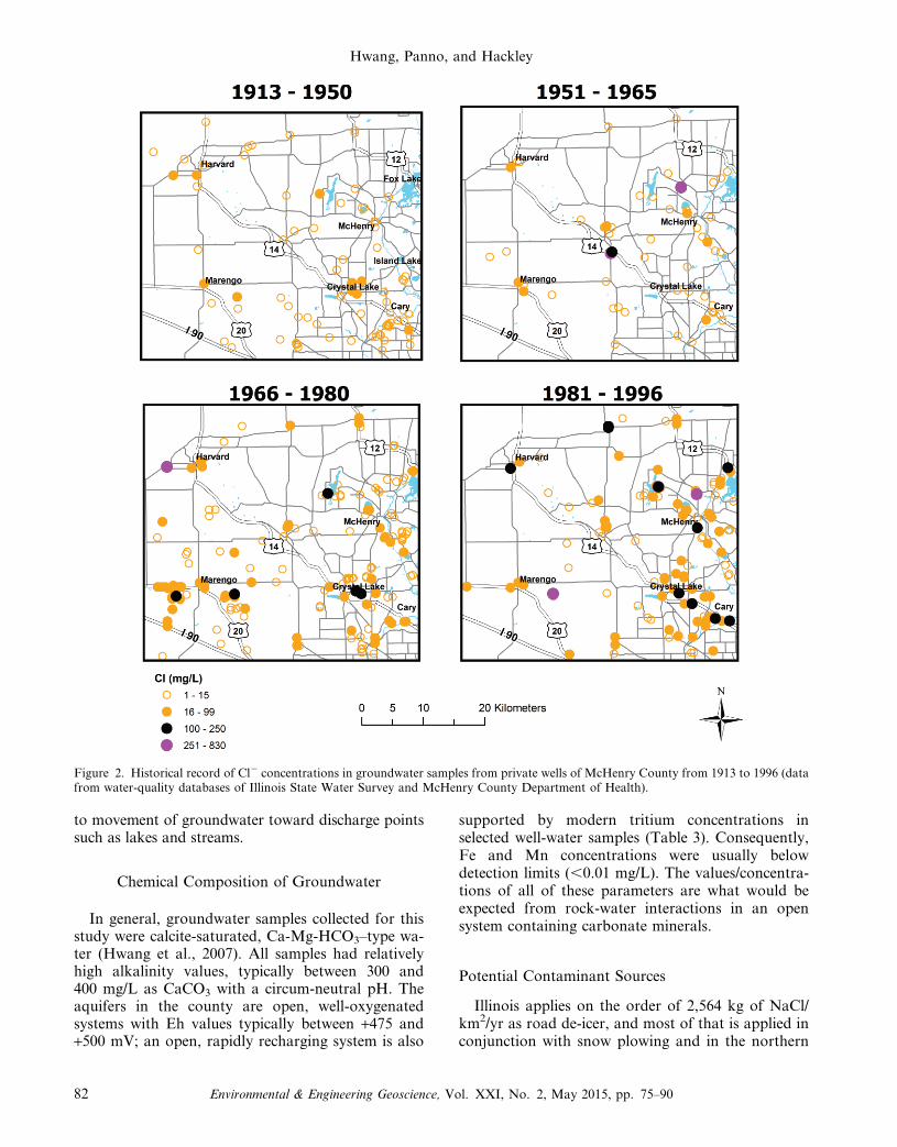
increased from the mid-1960s. Natural or backgroundCl2 concentrations in uncontaminated groundwater innorthern Illinois are between 1 and 15 mg/L (Panno etal., 2006a). Before 1951, only 15 percent of ground-water records contained Cl2 greater than 15 mg/L, andnone was above 100 mg/L (Figure 2). The percentageof records containing Cl2 greater than 15 mg/Lincreased to 20 percent for 1951 to 1965, 43 percentfor 1966 to 1980, and 51 percent for 1981 to 1996. AllCl2 data were divided into four depth intervalsbetween 0 and 61 m (Hwang et al., 2007). A higherpercentage of samples with Cl2 . 15 mg/L was foundin wells with depth 0 to 30 m (60 percent) than wellsgreater than 30 m (30 percent). Results of databaseanalysis indicated Cl2 concentration in groundwatergradually increased from 1913 to 1996. The higherpercentage of groundwater records with elevated Cl2

in shallower wells also suggests the source of chloridecontaminants are surface-borne.

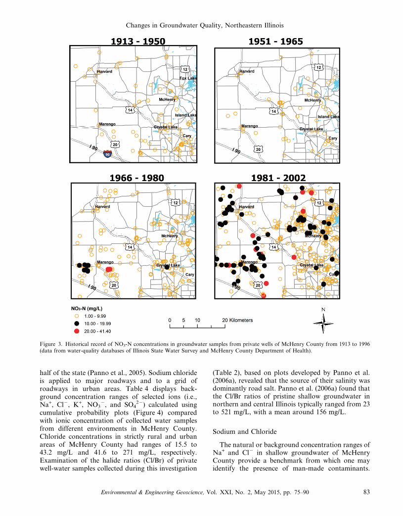
In the study area, NO32 concentrations in ground-

water increased from the mid-1960’s (Figure 3). Thistiming coincided with the period of rapid populationgrowth in McHenry County, and the period when

synthetic fertilizers began to be widely used byfarmers for growing crops in United States (Appeloand Postma, 1994). Other potential sources includenatural fauna, and wastes from humans (septiceffluent) and livestock (as discharge or fertilizer)(Panno et al., 2006a). Database analysis revealed that33 percent of records with depth less than 15 mcontained NO3

2 concentration greater than 10 mg/L.This percentage decreases to below 10 percent fordepths 15 to 30 m, and 2 percent for depths greaterthan 60 m. Such an inverse correlation between NO3-N concentrations and depth suggests a surface-bornecontaminant (Hwang et al., 2007).

The distribution of elevated NO32 concentrations on

a land-cover map (Illinois Department of Agriculture,2000) revealed a correlation between elevated NO3-Nconcentration ($10 mg/L) and areas of cropland(Hwang et al., 2007). This correlation suggests thatnitrogen compounds applied or produced in associa-tion with agricultural activities may be the majorsources of NO3

2 in shallow groundwater for McHenryCounty. In some cases, elevated NO3

2 was also foundin proximity to lakes and rivers, which is probably due

Table 3. Isotope data (units: per mil for stable isotopes, TU for tritium).

Sample ID dD d18O d13C (HCO32) d18O (NO3

2) d15N (NO32) d15N (NH4

+) Tritium

1 254.5 28.35 212.27 8.1 7.5 ND 8.292 255.9 28.45 212.78 ND ND ND 6.663 261.4 29.10 211.36 7.7 6.0 ND ND4 ND ND ND ND ND ND ND5 251.4 27.80 210.13 7.8 7.8 ND 8.736 259.3 28.98 213.08 5.3 4.2 ND ND7 250.1 27.78 28.63 5.6 3.3 ND ND8 253.2 28.17 213.98 4.1 8.6 ND 7.069 253.9 28.33 210.12 8.2 7.7 ND ND

10 255.9 28.65 213.32 5.8 8.9 ND ND11 258.1 28.78 211.69 7.8 6.1 ND ND12 260.4 29.04 211.92 6.2 5.9 ND ND13 256.9 28.60 210.62 8.7 7.6 ND ND14 256.9 28.86 210.40 7.7 5.1 ND 6.5115 256.5 28.90 29.96 8.9 5.7 ND 9.6916 257.6 28.50 213.31 6.0 9.0 ND 9.6717 257.1 28.46 211.00 ND ND ND 16.2918 256.2 28.47 29.03 13.5 22.9 ND 8.5719 ND 28.33 213.08 6.1 8.0 ND ND20 257.1 28.84 212.08 5.0 3.8 ND ND21 253.8 28.39 25.22 ND ND 23.2 ND22 255.9 28.75 211.37 4.2 5.1 ND ND23 250.9 28.00 212.39 5.0 10.4 ND ND24 228.3 21.99 25.96 ND ND 12.5 ND25 249.0 28.57 25.04 10.1 11.8 ND ND26 251.3 28.09 24.73 7.5 6.9 ND ND27 245.6 27.06 211.63 16.7 40.1 ND ND28 247.6 27.17 211.46 ND ND 7.7 ND29 250.9 27.89 28.87 5.2 2.7 ND ND30 242.6 26.74 216.14 8.3 12.9 ND ND31 248.7 26.70 23.82 6.8 3.4 ND ND

ND 5 not determined, mostly due to concentration that was too low to be analyzed for isotopic ratio.



to movement of groundwater toward discharge pointssuch as lakes and streams.

Chemical Composition of Groundwater

In general, groundwater samples collected for thisstudy were calcite-saturated, Ca-Mg-HCO3–type wa-ter (Hwang et al., 2007). All samples had relativelyhigh alkalinity values, typically between 300 and400 mg/L as CaCO3 with a circum-neutral pH. Theaquifers in the county are open, well-oxygenatedsystems with Eh values typically between +475 and+500 mV; an open, rapidly recharging system is also

supported by modern tritium concentrations inselected well-water samples (Table 3). Consequently,Fe and Mn concentrations were usually belowdetection limits (,0.01 mg/L). The values/concentra-tions of all of these parameters are what would beexpected from rock-water interactions in an opensystem containing carbonate minerals.

Potential Contaminant Sources

Illinois applies on the order of 2,564 kg of NaCl/km2/yr as road de-icer, and most of that is applied inconjunction with snow plowing and in the northern

Figure 2. Historical record of Cl2 concentrations in groundwater samples from private wells of McHenry County from 1913 to 1996 (datafrom water-quality databases of Illinois State Water Survey and McHenry County Department of Health).



half of the state (Panno et al., 2005). Sodium chlorideis applied to major roadways and to a grid ofroadways in urban areas. Table 4 displays back-ground concentration ranges of selected ions (i.e.,Na+, Cl2, K+, NO3

2, and SO422) calculated using

cumulative probability plots (Figure 4) comparedwith ionic concentration of collected water samplesfrom different environments in McHenry County.Chloride concentrations in strictly rural and urbanareas of McHenry County had ranges of 15.5 to43.2 mg/L and 41.6 to 271 mg/L, respectively.Examination of the halide ratios (Cl/Br) of privatewell-water samples collected during this investigation

(Table 2), based on plots developed by Panno et al.(2006a), revealed that the source of their salinity wasdominantly road salt. Panno et al. (2006a) found thatthe Cl/Br ratios of pristine shallow groundwater innorthern and central Illinois typically ranged from 23to 521 mg/L, with a mean around 156 mg/L.

Sodium and Chloride

The natural or background concentration ranges ofNa+ and Cl2 in shallow groundwater of McHenryCounty provide a benchmark from which one mayidentify the presence of man-made contaminants.

Figure 3. Historical record of NO3-N concentrations in groundwater samples from private wells of McHenry County from 1913 to 1996(data from water-quality databases of Illinois State Water Survey and McHenry County Department of Health).



Sodium is a non-conservative ion and is derived fromrainwater and snowmelt at present-day concentra-tions of about 0.06 mg/L (NADP, 2012). Thisconcentration can increase with evapotranspiration(roughly 70 percent in Illinois) to about 0.2 mg/L. Ionexchange with Ca2+ in the soil zone would decreasethe concentration of Na+ below what would beexpected based on Cl2 concentrations. Anthropogen-ic sources, which includes wastes from humans (septiceffluent) and livestock in rural areas, manure appliedas fertilizer in rural areas, and road de-icers (NaCl) inboth rural and urban areas (Panno et al., 2006a), cangreatly increase the concentration of Na+ and Cl2 ingroundwater.

Inflection points for Na+ on the cumulativeprobability graph include 1.6 mg/L and 24.5 mg/L(Figure 4). The background concentration range,from ,0.1 to 1.6 mg/L, is near the lower end of therange found at Sterne’s Woods Fen located east ofCrystal Lake in McHenry County by Panno et al.(1999) using the same technique (,1 to 10 mg/L).Because of the limited scale of that study, and thegreater number of samples and broader range ofsample locations for this investigation, we estimatepre-settlement background at between 1.6 and 24 mg/L. We suggest that Na+ concentrations .24 (roundedto two significant figures) are an effect of urbaniza-tion and the use of road de-icers and are consistentwith Na+ concentrations in well-water samplescollected after 1960 identified by Hwang et al.

(2007). Sodium concentrations in groundwater abovethe inflection point of 24.5 mg/L are interpreted as aneffect of sampling in both rural and urban areas. Thatis, groundwater in urban areas typically has a greaterNa+ concentration than rural counterparts due to agreater concentration of roadways. Therefore, Na+

concentrations .24 mg/L are probably indicative ofcontamination by manure fertilizer, livestock, and/orroad salt applied to roadways. The greatest concen-trations of Na+ were found in wells sampled after1960, when road salt was used routinely.

Chloride is a conservative ion and is derived fromrainwater and snowmelt at present-day concentrationsof about 0.1 mg/L (NADP, 2012). This concentrationcan increase with evapotraspiration to about 0.33 mg/Lin Illinois. Added to this is Cl2 from natural fauna androck-water interaction in pristine areas. Anthropogenicsources, including wastes from humans (septic effluent,water softeners) and livestock in rural areas, soilamendments (KCl) and manure applied as fertilizer inrural areas, and road de-icers (NaCl) in both rural andurban areas (Panno et al., 2006a), can greatly increasethe concentration of Cl2 in groundwater.

Inflection points for Cl2 on the cumulativeprobability graph include 5.7 mg/L, 45 mg/L, and107 mg/L (Figure 4). The lowest range of concentra-tions (0.1 to 5.7 mg/L) is somewhat lower than thatdetermined by Panno et al. (2006a) (i.e., 0.1 to 15 mg/L) using another technique. Bartow et al. (1909)found that the majority of wells screened in glacial

Table 4. Range of selected ionic concentration in groundwater from different environments with background range using cumulative probabilityplots (unit: mg/L).

Component Environment Range Mean Median Background Range

Na+ Urban 23.8–191 92.6 80Rural 3.1–53.5 16.8 10.7 1.6–24Urban/rural* 3.2–99.4 37.3 34.5Livestock 3.8–26.7 14.8 15.8

K+ Urban 2–7 5 6Rural 4–119 27.2 4 1.15–3.6Urban/rural 4–9 6.8 7Livestock 4–87 25.4 5

Cl2 Urban 41.6 to 271 152.8 166Rural 15.5 to 43.2 24.1 21.5 0.1–5.7Urban/rural 2.8 to 164 72.9 59.4Livestock 15.4 to 69.2 37.8 35.4

NO32 Urban 0.1 to 14.2 6.9 7.3

Rural 0 to 49 13.7 9.6 0.44–1.7Urban/rural 0 to 12.1 5.7 5.5Livestock 0 to 25.4 15.8 18.7

SO422 Urban 26.2 to 76.4 42.9 42.1

Rural 4.8 to 57.9 28 24.9 0.1–35{Urban/rural 1.3 to 56.3 30 34.3Livestock 15.2 to 236 66.2 37.6

*Near border of urban and rural areas.{Estimated background range.



drift in Illinois contained less than 15 mg/L of Cl2. Theconcentration range from .5.7 to 45 mg/L shares thesame upper bound as that found in Sterne’s WoodsFen in McHenry County (Panno et al., 1999) using thecumulative probability technique. Based on the graph-ical results, we estimate pre-settlement backgroundfor Cl2 at between 0.1 and 5.7 mg/L. Groundwatercontaminated with manure fertilizer, livestock effluent,and potash probably ranges from .5.7 to 45 mg/L.The highest range (.45 to 107 mg/L) is an effect ofurbanization and the use of road de-icers and isconsistent with Cl2 concentrations in well-watersamples collected after 1960 (Hwang et al., 2007).Groundwater in urban areas typically has a greaterCl2 concentration than its rural counterpart due toa greater concentration of roadways. The greatestconcentration of Cl2 (between 107 and 830 mg/L) wasfound in wells sampled between 1966 and 1996primarily along major roadways in and around thevicinity of large towns in McHenry County.

Nitrate

Nitrate is derived from rainwater and snowmelt atpresent-day concentrations of about 0.35 mg/L (as N)(NADP, 2012); these concentrations can increase,with evapotraspiration, to as much as 1.2 mg/L.Added to this is NO3

2 from natural fauna, plusanthropogenic sources, which include wastes fromhumans (septic effluent) and livestock, and N-basedfertilizers (mostly anhydrous ammonia) and manure,applied as fertilizer, in rural areas (Panno et al.,2006b). Unlike the more conservative Cl2, NO3

2 isreactive and is often taken up by plants and, underreducing conditions, will undergo bacterially mediat-ed denitrification that will convert it to nitrogen gas.

Inflection points on the cumulative probabilitygraph include 0.8 mg/L (a very large inflection point),0.43 mg/L, 1.7 mg/L, and 22 mg/L (Figure 4). Theinitial range of between 0.01 and 0.08 mg/L isprobably very dilute groundwater, reflecting NO3

2

Figure 4. Background concentrations of Na+ (n 5 380), K+ (n 5 262), Cl2 (n 5 755), and NO3-N (n 5 680) in the sand and gravel aquifersof McHenry County, Illinois, based on cumulative probability plots of historic and recent groundwater chemistry data.



concentrations of rainwater and snowmelt. The rangebetween .0.08 and 0.43 mg/L is probably indicativeof evaporative/evapotranspiration concentration ofNO3

2. This is consistent with work by Bartow et al(1909), who found that the majority of wells in theglacial sediment in Illinois at the end of the nineteenthcentury contained less than 0.4 mg/L NO3

2. Therange between 0.44 mg/L and 1.7 mg/L reflectspresent-day background concentrations in areas notimpacted by modern agriculture (Table 4), and therange is similar to that determined by Panno et al.(2006b) for NO3

2 in a southwestern Illinois sinkholeplain of 0.1 to 2.1 mg/L. Nitrate-N concentrationsexceeding 1.7 mg/L probably reflect the effects ofapplication of N-fertilizer, which became popularafter 1960 (e.g., Panno et al., 2006b). This isconsistent with Hwang et al. (2007), who identifieda steady increase in NO3

2 in the rural areas ofMcHenry County after 1966. The greatest concentra-tions of NO3

2 (up to 49 mg/L) are found in wells lessthan 10 m deep from rural areas of McHenry Countyafter 1970, which are probably associated withlivestock effluent.

Potassium

Potassium is a naturally occurring ion in ground-water and may be derived from chemical weatheringof K-rich feldspars and micas during rock-waterinteraction (Hem, 1985), all of which are present inthe sand and gravel aquifer materials in northernIllinois (e.g., Hackley et al., 2010). Potassium inrainwater is typically very low in concentration, onthe order of 0.02 mg/L in Illinois (NADP, 2012).Because K+ is efficiently sequestered by plants as anutrient and tends to be reincorporated into clayminerals (e.g., illite), K+ concentrations are typicallylow in groundwater (in the low single digits).Anthropogenic sources, such as K-based fertilizers(KCl), as well as livestock and human waste, canincrease the concentration of K+ to concentrationstypically greater than 5 but typically less than 15 mg/L (Panno et al., 2006a) (Table 1). Potassium concen-trations in McHenry County groundwater range from0.3 to 13 mg/L. However, two well-water samples inthe ISWS database had K+ concentrations of 50 and213 mg/L, which are a factor of 4 and 16 greater thanthe next highest concentration, suggesting eitherhighly localized contamination of these wells (e.g.,by potash) or a transcription error in the historicdata. Neither was used in the background calcula-tions, and their exclusion had no effect on thedetermination of background concentrations.

Inflection points for K+ on the cumulative proba-bility graph include 1.14 and 3.60 mg/L (Figure 4 and

Table 4). Such levels were observed in the row-crop–rich terrain of southwestern Illinois, where K+

concentrations ranged from ,1 to 3 mg/L in well-water samples, and ,1 to as high as 7 mg/L in spring-water samples. The greatest concentrations werefound in the fall of the year (Hackley et al., 2007).Bartow et al. (1909) found that K+ concentrationsexceeding 5.0 mg/L in springs and wells screened inglacial drift in Illinois were uncommon. We observedthree populations of K+ concentrations: the lowestconcentration range (0.1 to 1.14 mg/L) probablyrepresents pre-settlement background concentrations;the concentration range from .1.14 to 3.6 mg/Lrepresents present-day background concentrations;concentrations of K+ greater than 3.6 mg/L representelevated concentrations from the application of K-based soil amendments and discharge of livestockwaste and septic effluent. The inflection point at9.4 mg/L is an artifact of the cumulative probabilityplot (sparse data) and should be ignored.

Sulfate

Sulfate concentrations ranged from 14 to 64 mg/Lbut were generally between 35 and 45 mg/L; an upperbackground threshold for SO4

22 was estimated byPanno (ISGS, unpublished data) to be about 35 mg/Lbased on hundreds of shallow groundwater samplesfrom throughout Illinois (Table 4). The effects ofland-use changes (e.g., excavation, plowing, N-fertilizer application) can increase the SO4

22 concen-trations as a result of the exposure and oxidation ofpyrite within glacial tills, the anaerobic oxidation ofpyrite in the presence of NO3

2 (Appelo and Postma,1994), and the interaction of oxidation products withcarbonate minerals within the aquifers and tills.

Aquifer Susceptibility

Because of the open nature of the sand and gravelaquifers, groundwater in McHenry County can easilybe contaminated with surface-borne pollutants. Anaquifer sensitivity map (Keefer, 1995) showed thatthe uppermost sand and gravel aquifers in manyplaces of the McHenry County are highly susceptibleto contamination by NO3-N leaching; soil leachingindices in many areas of the county were described as‘‘very fast’’ to ‘‘fast.’’

Modern groundwater collected by this studyreveals elevated concentrations of Na+, Cl2, K+,and NO3

2 (Table 4). Elevated Na+ and Cl2 concen-trations in groundwater were encountered in bothrural and urban areas, but concentrations werehighest immediately adjacent to major roadwaysand in urban areas where there was a high density



of roadways. Road salt was the most likely source ofNa+ and Cl2 contamination based on Cl/Br ratios ofgroundwater with elevated Cl2 (Table 2). Sodiumand Cl2 concentrations in urban areas were as high as191 and 271 mg/L, respectively, almost 20 times thatof background (Table 4). Groundwater in rural areasalso had concentrations of Na+ and Cl2 well abovebackground levels but typically at lower concentra-tions than in urban areas. Concentrations of K+ inMcHenry County groundwater were relatively high,ranging from 0.6 to 8.2 mg/L; K+ in uncontaminatedgroundwater in this county ranged from ,0.6 and3.6 mg/L, with a median concentration of 2.1 mg/L(Panno et al., 1999). The dominant source of K+ inthis county is probably KCl and other K-containingsoil amendments and fertilizers applied to thecroplands.

Nitrate concentrations from urban areas weretypically elevated (0.1 to 14.2 mg/L), but concentra-tions were low relative to NO3

2 concentrations inrural areas (,0.1 to 49 mg/L; Table 4). Nitrateconcentrations in the vicinity of livestock operationswere as high as 25.4 mg/L. Nitrate isotope data fromselected wells confirmed that the dominant sourceof NO3

2 was N-fertilizer. Elevated NO32 concentra-

tions also correlated well with areas of greaterleaching potential on an aquifer sensitivity mapto nitrate leaching by Keefer (1995) (Figure 10of Hwang et al., 2007). This correlation supportssurface-borne contaminant sources for NO3

2.

Isotopic Composition of Collected Water

dD and d18O of Water

Water samples collected for this study wereanalyzed for various isotopic ratios. The dD valuesof water ranged from 241.6 to 261.4 per mil, and thed18O values ranged from 26.7 to 29.1 per mil(Hwang et al., 2007). Most of the data fall on themeteoric line on a dD vs. d18O plot. The leachatesample from a horse manure pile had much higher dDand d18O values (228.3, 21.99 per mil). Since theleachate sample was collected from a small puddlenext to the standing horse manure pile on the ground,higher dD and d18O values may reflect the effect ofevaporation.

d15N and d18O of Dissolved Nitrate

NO32 isotopes were examined to determine nitrate

sources. The d15N values of nitrate ranged from 2.7 to40.1 per mil, and the d18O values ranged from 4.1 to16.7 per mil (Hwang et al., 2007). Based on theisotopic data, the predominant sources of NO3

2 in

the shallow groundwater samples are fertilizer andsoil organic matter, despite the fact that the sampleswere collected from different environments, such asurban, rural, and livestock farms. Although severalsamples were collected near farms with livestockfacilities, the only one with clear indication ofmanure/septic source was sample 27, which had thelargest d15N (+40.1 per mil) and d18O (+16.7 per mil)values. The lack of an isotopic signature of manurefor most of the livestock farm groundwater samplesmay be due to the widespread nature of croplandssurrounding those operations, which caused theisotopic signature of manure to be diluted by thatof fertilizer and soil organic nitrogen. Fertilizerapplication on urban lawns and parks may result inthe isotopic signature of fertilizer and soil nitrogen inurban areas.

A few samples showed enriched d15N and d18Ovalues following the denitrification trajectory (Fig-ure 5), which suggests that they have undergonevarious degrees of denitrification. A negative correla-tion was observed between d13C and d15N (Figure 6),which is consistent with the denitrification process;that is, in an anaerobic environment, micro-organismsserve as denitrifiers and reduce NO3

2 to oxidizeorganic carbon or sulfide in the following reactions(Batchelor and Lawrence, 1978; Kendall, 1998):

4NO{3 z5Cz2H2O?2N2z4HCO{

3 zCO2 ð1Þ

14NO{3 z5FeS2z4Hz?

7N2z10SO2{4 z5Fe2zz2H2O

ð2Þ

Figure 5. d18O vs. d15N showing that the predominant sourcesof NO3

2 are N-fertilizer and soil organic matter, and thatdenitrification is actively occurring within the soil zone and/oraquifers (modified from Clark and Fritz, 1997).



Denitrification reactions cause both the d15Nand d18O of the residual NO3

2 to increase becausemicro-organisms preferentially consume 14N relativeto 15N, and 16O relative to 18O. Denitrificationthrough reaction 1 could also cause the d13CDIC inHCO3

2 to decrease because the organic carbon,which would be oxidized to form HCO3

2, typicallyhas much lower d13C values. In reaction 2, whileNO3

2 is reduced (denitrified), FeS is oxidized to formSO4

22, which should result in an increase in SO422

concentration. A positive correlation between SO422

concentration and d15N, as a result of denitrificationprocess, showing N and O isotope evidence ofdenitrification was observed by Hwang et al. (2007).

d15N of Ammonia

Only three samples that contained enough ammo-nia were analyzed for ammonia d15N. The firstsample was collected from a shallow well in whichgroundwater was under reducing conditions, and forwhich Cl2 and NH4

+ (as N) concentrations were only2.8 and 1.98 mg/L, respectively (well within back-ground). This sample’s d15N value was 23.2 per miland fell within the range of soil organic matter(Figure 5). The second sample was from a shallow(0.8 m deep) hand-dug well down gradient from a hogfarm with elevated Cl2 and NH4

+-N concentrationsof 56.5 and 21.8 mg/L, respectively. The d15N valuefor the dug well was +7.7 per mil and within the rangeof animal waste. The third sample consisted of horsemanure leachate and was enriched in Na+ and Cl2,

and all nutrients (Table 1), and had a d15N value of+12.5 per mil (indicative of animal waste; Figure 5).

Tritium Content in Water

Tritium analyses were completed for six ground-water samples collected from depths of 6 to 30 m. Thetritium measurements ranged predominantly from 6.5to 9.7 TU, with one sample containing 16.29 TU.These tritium data imply that groundwater in thestudy area is relatively young, having a travel timefrom recharge to well depths of between less than oneand 30 years. Most of the tritium values fall within orclose to the range expected for recent precipitation,which is approximately 2 to 8 TU (Eberts andGeorge, 2000; Hackley et al., 2007; and Warrier etal., 2013). The greater tritium levels measured for wellsite 17 may represent slightly older groundwatercloser to 1960s values. Well site 17 also contained verylittle NO3

2 (0.19 mg/L), suggesting less immediateimpact from surface infiltration. This well wasscreened in a very thin lens of sand sandwichedbetween a relatively thick tight till (Hwang et al.,2007), whereas all the other wells were screenedin significantly thicker sand/gravel deposits, whichundoubtedly have a more direct hydraulic connectionto the land surface.

CONCLUSIONS

Temporal analysis of the groundwater qualitydatabases revealed that Cl2 and NO3

2 concentrationsin shallow groundwater from McHenry County haveincreased considerably from the mid-1960s to 2003.This time period coincides with rapid populationgrowth in McHenry County. Database analysis alsorevealed higher percentage of elevated Cl2 and NO3

2

concentrations in wells shallower than 30 m in depth.The correlation of higher ionic concentration withshallower wells, and their relationship with calculatedand estimated background concentrations of selectedions (Na+, K+, Cl2, NO3

2, and SO422) indicate that

the sources of increased ionic concentrations weresurface-borne. It is likely that Cl concentrations arethe result of yearly application of road salt in urbanareas. This is supported by Panno et al. (2005, 2006a),who, using Cl/Br ratios from the same samples,showed that groundwater samples collected duringthis present investigation were contaminated withhalite. Rapid population growth in McHenry Countysince 1970 has resulted in expansion of urban areasand has resulted in more applications of road salt inwinter seasons. Greater NO3

2 concentrations prob-ably resulted from increased fertilizer use, given thatextensive applications of fertilizer began in the 1960s.

Figure 6. d13C vs. d15N showing an inverse correlation that isconsistent with microbially mediated denitrification. Two popu-lations are visible here, one dominated by animal waste (uppertrend), and a more clustered lower trend.



Positive correlation between greater NO32 concen-

trations and areas of greatest leaching potential,shown on an aquifer sensitivity map, supports thehypothesis that non-point, surface-borne sourceswere responsible for NO3

2 contamination.Groundwater chemistry data from groundwater

samples revealed that urban groundwater containedhigher Na+ and Cl2 concentrations, and ruralgroundwater contained greater NO3

2 concentrations.Such association of specific ionic concentrations andenvironments illustrates the effect of land use ongroundwater quality.

Results of isotope analyses indicated that thepredominant NO3

2 sources are fertilizer and soilorganic nitrogen, from crop-related agriculturalpractices. This is to be expected for a county inwhich land use is dominated by croplands. Sinceprivate septic systems are common in rural areas,septic effluent may affect some of the shallowgroundwater. However, from the 30 samples col-lected, there was no isotopic evidence of influencefrom septic systems. A more detailed sampling arraynear septic discharge systems would be needed toevaluate septic input to the shallow groundwatersystem. Isotope results did detect the influence oflivestock manure as a source of NO3

2 at one location.Because there are many small-scale farms withlivestock in McHenry County, its influence may bemore prevalent, albeit localized, than what weobserved from our data. Effects of denitrificationwere observed in groundwater from a few samples asindicated by the generally positive d15N and d18Otrends for NO3

2 and the negative correlation betweend13C of HCO3

2 and the d15N of NO32.

ACKNOWLEDGMENTS

This research was supported by a grant fromthe Illinois Groundwater Consortium under AwardNo. A8634 and by the Illinois State GeologicalSurvey. The authors thank the Illinois State WaterSurvey and the McHenry County Department ofHealth for providing historical water-quality data-bases. Publication of this article has been authorizedby the director of the Illinois State Geological Survey,Prairie Research Institute, University of Illinois.

REFERENCES

APPELO, C. A. AND POSTMA, D., 1994, Geochemistry, Groundwater

and Pollution: A. A. Balkema Publishers, Leiden, Nether-

lands.

BARTOW, E.; UDDEN, J. A.; PARR, S. W.; AND PALMER, G. T., 1909,

The Mineral Content of Illinois Waters: Illinois State

Geological Survey Bulletin 10, 1–192.

BATCHELOR, B. AND LAWRENCE, A. W., 1978, A kinetic model forautotrophic denitrification using elemental sulfur: Water

Research, Vol. 12, pp. 1075–1084.

CLARK, I. AND FRITZ, P., 1997, Environmental Isotopes in

Hydrogeology: CRC Press, New York, 328 p.

COLEMAN, M. L.; SHEPARD, T. J.; ROUSE, J. J.; AND MOORE, G. R.,

1982, Reduction of water with zinc for hydrogen isotopeanalysis: Analytical Chemistry, Vol. 54, pp. 993–995.

CSALLANY, S. AND WALTON, W. C., 1963, Yields of Shallow

Dolomite Wells in Northern Illinois: Illinois State WaterSurvey Report of Investigation 46, 43 p.

CURRY, B. B.; BERG, R. C.; AND VAIDEN, R. C., 1997, Geologic

Mapping for Environmental Planning, McHenry County,

Illinois: Illinois State Geological Survey Circular 559.

EBERTS, S. M. AND GEORGE, L. L., 2000, Regional Ground-Water

Flow and Geochemistry in the Midwestern Basins and Arches

Aquifer System in Parts of Indiana, Ohio, Michigan and

Illinois: U.S. Geological Survey Professional Paper 1423-C,103 p.

EISEN, C. AND ANDERSON, M., 1979, The effect of urbanization ongroundwater quality—A case study: Ground Water, Vol. 17,pp. 456–462.

EPSTEIN, S. AND MAYEDA, T., 1953, Variation of 18O content of

waters from natural sources: Geochimica et Cosmochimica

Acta, Vol. 4, pp. 213–224.

HACKLEY, K. C.; LIU, C. L.; AND TRAINOR, D., 1999, Isotopicidentification of the source of methane in subsurfacesediments of an area surrounded by waste disposal facilities:Applied Geochemistry, Vol. 14, pp. 119–131.

HACKLEY, K. C.; PANNO, S. V.; HWANG, H.-H.; AND KELLY, W. R.,2007, Groundwater Quality of Springs and Wells in the

Sinkhole Plain in Southwestern Illinois: Determination of the

Dominant Sources of Nitrate: Illinois State Geological SurveyCircular 570, 1–39.

HACKLEY, K. C.; PANNO, S. V.; AND JOHNSON, T. F., 2010,Chemical and isotopic indicators of groundwater evolution inthe basal sands of a buried bedrock valley in the Midwestern

United States: Implications for recharge, rock-water interac-tions and mixing: Geological Society of America Bulletin,Vol. 122, pp. 1047–1066.

HALLBERG, G. R. AND KEENEY, D. R., 1993, Nitrate. In Alley, W.(Editor), Regional Ground-Water Quality: Van NostrandReinhold, New York. pp. 297–322.

HEM, J. D., 1985, Study and Interpretation of the Chemical

Characteristics of Natural Water: U.S. Geological Survey

Water-Supply Paper 2254.

HERZOG, B. L.; STIFF, B. J.; CHENOWITH, C. A.; WARNER, K. L.;

SIEVERLING, J. B.; AND AVERY, C., 1994, Buried Bedrock

Surface of Illinois: Illinois State Geological Survey Map 5,scale 1:500,000.

HORBERG, L., 1950, Bedrock Topography in Illinois: Illinois StateGeological Survey Bulletin 73, 111 p.

HWANG, H.-H.; LIU, C.-L.; AND HACKLEY, K. C., 1999, Methodimprovement for oxygen isotope analysis in nitrates. InGeological Society of America North-Central Section Meet-

ing, Abstracts with Programs, Vol. 31, No. 5, p. 12.

HWANG, H.-H.; PANNO, S. V.; AND HACKLEY, K. C., 2007, Chemical

and Isotopic Database for McHenry County Study on

Groundwater Quality and Land Use: Illinois State GeologicalSurvey Open-File Series OFS 2007-6.

ILLINOIS DEPARTMENT OF AGRICULTURE, 2000, Land Cover of Illinois

1999–2000: Electronic document, available at http://www.agr.state.il.us/gis/landcover99-00.html

KEEFER, D. A., 1995, Potential for Agricultural Chemical

Contamination of Aquifers in Illinois: 1995 Revision: Illinois



State Geological Survey Environmental Geology Series 148,

28 p.

KELLY, W. R., 2008, Long-term trends in chloride concentrations

in shallow aquifers near Chicago: Ground Water, Vol. 46,

pp. 772–781.

KENDALL, C., 1998, Tracing nitrogen sources and cycling in

catchment. In Kendall, C., and McDonnell, J. J. (Editors),Isotope Tracer in Catchment Hydrology: Elsevier Science

B.V., Amsterdam, Netherlands, 839 p.

LANDSBERGER, S.; O’KELLY, D. J.; AND PANNO, S. V., 2003,

Determination of bromine, chlorine and iodine in environ-

mental aqueous samples from epithermal neutron activationanalysis and Compton suppression: Transactions of the

American Nuclear Society, Vol. 89, pp. 735–736.

MEYER, S. C., 1998, Ground-Water Studies for Environmental

Planning, McHenry County, Illinois: Illinois State Water

Survey Contract Report 630, 141 p.

NADP, 2012, National Atmospheric Deposition Program: Elec-

tronic document, available at http://www.isws.illinois.edu/

hilites/nadp/

O’RIORDAN, T. AND BENTHAM, G., 1993, The politics of nitrate in

the UK. In Burt, T. P.; Heathwaite, A. L.; and Trudgill, S. T.

(Editors), Nitrate-Processes, Patterns and Management: JohnWiley and Sons, New York. pp. 57–68.

OSTLUND, H. G. AND DORSEY, H. G., 1977, Rapid electrolytic

enrichment and hydrogen gas proportional counting of

tritium. In Low-Radioactivity Measurements and Applications:

Proceedings of the International Conference on Low-Radioac-

tivity Measurements and Applications: October 6–10, 1975:

Slvenske Pedagogike Nakladetal’stvo, Bratislava, Slovakia.

pp. 95–104.

PANNO, S. V.; HACKLEY, K. C.; HWANG, H.-H.; GREENBERG, S.;

KRAPAC, I. G.; LANDSBERGER, S.; AND O’KELLY, D. J., 2005,

Characterization and Identification of the Sources of Na-Cl

in Groundwater and Surface Water, with Emphasis on the

Midwestern U.S.: Illinois State Geological Survey Open-File

Series 2005-1.

PANNO, S. V.; HACKLEY, K. C.; HWANG, H.-H.; GREENBERG, S.;

KRAPAC, I. G.; LANDSBERGER, S.; AND O’KELLY, D. J., 2006a,Characterization and identification of the sources of Na-Cl in

ground water: Ground Water, Vol. 44, pp. 176–187.

PANNO, S. V.; KELLY, W. R.; MARTINSEK, A.; AND HACKLEY, K. C.,

2006b, Estimating background and threshold nitrate concen-

trations using probability graphs: Ground Water, Vol. 44,pp. 697–709.

PANNO, S. V.; NUZZO, V.; CARTWRIGHT, K.; HENSEL, B. R.; AND

KRAPAC, I. G., 1999, Changes to the chemical composition ofgroundwater in a fen-wetland complex caused by urbandevelopment: Wetlands, Vol. 19, pp. 236–244.

RAVEH, A. AND AVNEMELECH, Y., 1979, Total nitrogen analysis inwater, soil and plant material with persulfate oxidation:Water Research, Vol. 13, pp. 911–912.

SILVA, S. R.; KENDALL, C.; WILKISON, D. H.; ZEIGLER, A. C.;CHANG, C. C. Y.; AND AVANZINO, R. J., 2000, A new methodfor collection of nitrate from fresh water and the analysis ofnitrogen and oxygen isotope ratios: Journal of Hydrology,Vol. 228, pp. 22–36.

STRELLIS, D. A.; HWANG, H.-H.; ANDERSON, T. F.; AND LANDS-

BERGER, S., 1996, A comparative study of IC, ICP-AES andNAA measurements of chlorine, bromine and sodium innatural waters: Journal of Radioanalytical and NuclearChemistry, Vol. 211, pp. 473–484.

SUTER, M.; BERGSTROM, R. E.; SMITH, H. F.; EMRICH, G. H.;WALTON, W. C.; AND LARSON, T. E., 1959, Preliminary Reporton Ground-Water Resources of the Chicago Region, Illinois:Illinois State Water Survey Cooperative Ground-WaterReport 1, 89 p.

U.S. CENSUS BUREAU, 2000, Census of Population: U.S. CensusBureau, Washington, DC.

U.S. CENSUS BUREAU, 2010, Census of Population: U.S. CensusBureau, Washington, DC.

VENNEMANN, T. W. AND O’NEIL, J. R., 1993, A simple andinexpensive method of hydrogen isotope and water analysesof minerals and rocks based on zinc reagent: ChemicalGeology, Vol. 103, pp. 227–234.

VISOCKY, A. P.; SHERILL, M. G.; AND CARTWRIGHT, K., 1985,Geology, Hydrogeology, and Water Quality of the Cambrianand Ordovician Systems in Northern Illinois: Illinois StateGeological Survey and Illinois State Water Survey Cooper-ative Groundwater Report 10.

WARRIER, C. U.; BABU, M.; MANJULA, P.; AND HAMEED, A. S.,2013, Spatial and temporal variations of natural tritium inprecipitation of southern India: Current Science, Vol. 105,No. 2, pp. 242–248.

WOLLER, D. M. AND SANDERSON, E. W., 1976, Public GroundwaterSupplies in McHenry County: Illinois State Water SurveyBulletin 60.

WOOD, W. W., 1981, Guidelines for collection and field analysis ofground-water samples for selected unstable constituents. InTechniques of Water-Resources Investigations of the U.S.Geological Survey, Book 1, Chap. D2. 24 p.



Sorption-Desorption Characteristics of

Tetrabromobisphenol A on Humin and Sediment of

Lake Chaohu, China

SUWEN YANG1

SHENGRUI WANG

BINGHUI ZHENG

FENGCHANG WU

State Key Laboratory of Environmental Criteria and Risk Assessment,Lake Research Center, Chinese Research Academy of Environmental Sciences,

Anwai Dayangfang 8-1, Chaoyang District, Beijing 100012, China

QIANG FU

Environmental Monitoring Quality Control Department, China NationalEnvironmental Monitoring Center, Anwai Dayangfang 8-2, Chaoyang District,

Beijing 100012, China

Key Terms: Tetrabromobisphenol A, Sorption-Desorption,Sediment, Chaohu Lake

ABSTRACT

Three components of sediments with regard to thesorption-desorption characteristics of tetrabromobi-sphenol A (TBBPA) in sediment water systems wereinvestigated. Results show that the Freundlich andLangmuir model can describe the sorption behavior ofTBBPA well. The calculated Cmax (maximum unitsorption quantity) values were 1.47, 2.13, and 3.65 mg/kg for mineral group (MG), clay group (CG), andhumin group (HG) sediments, respectively. HG exhib-ited a stronger nonlinear behavior than did CG andMG. The order of sorption capability was as follows:HG . CG . MG. Desorption capability order was theopposite. Simultaneously, it was found that precipita-tion was the main sorption type for TBBPA onsediment. The contribution of precipitation sorptionranged from 45 percent to 70 percent within a TBBPAconcentration ranging from 0.1 to 10.0 mg/L in thesupernatant. This may be attributable to anomalouschanges in the compounds’ ionic activity in combinationwith metal cations. Sorption-desorption experiments onclay sediment were also conducted at pH levels rangingfrom 3 to 14 and temperatures ranging from 46C to306C. In this regard, the sorption of TBBPA decreasedas pH and temperature increased gradually. Further-

more, sorption and desorption reached a dynamicequilibrium at pH 11.5 and at a temperature of 306C,respectively. The release of TBBPA from sedimentwould be higher in summer than in the three otherseasons, which may pose a potential ecological risk foraquatic life in lakes.

INTRODUCTION

Tetrabromobisphenol A (TBBPA) is one of the mostwidely used brominated flame retardants (BFRs).Annual output of TBBPA in 2000 was 8,000 tons,which accounted for 76 percent of the total BFRs inChina (Sun et al., 2008a). The demand for BFRs inChina has increased by 8 percent per year recently (Shiet al., 2009). Lake Chaohu (Anhui Province) is one ofthe main production sites for BFRs in China (Jin et al.2008; Xu et al. 2009). As the main BFR with respect toproduction and consumption, TBBPA can be releasedinto the environment (Morris et al., 2004). Previousstudies suggest that TBBPA is toxic to a variety oforganisms (Darnerud, 2003), especially aquatic animals(Janer et al., 2007; Johnson-Restrepo et al., 2008).Therefore, it may pose a potential risk to the aquaticecosystem (WHO/ICPS, 1995; Veldhoen et al., 2006;Liu and Zhou, 2008; and Nyholm et al., 2008).Scientists and governments worldwide have beencommitted to investigating TBBPA content in theenvironment as well as its movement, exposure toxicity,and metabolism in vivo in order to make appropriateregulatory recommendations (Kemmlein et al., 2003).1Corresponding author email: [email protected].


TBBPA has been detected in various environmentaland biota matrixes such as soil (Ravit et al. 2005; Xuet al., 2012), air (Jakobsson et al., 2002), sediment(Qu et al., 2011; Zhang et al., 2011; Feng et al., 2012),aquatic organisms (Leist et al., 2009; Yang et al.,2012; and He et al., 2013), and the human body(Cariou et al., 2008; Abdallah and Harrad, 2011;Mohamed and Abdallah, 2011; and Shi et al., 2013).The maximum TBBPA concentration in sedimentfrom Lake Chaohu has already reached 518.3 ng/g(Yang et al., 2012), which is almost the highest valuein the world. Thus, it may pose a potential danger tothe aquatic ecosystem (WHO/ICPS, 1995; Nyholm etal., 2008; Debenest et al., 2010; and Yang et al., 2013).Furthermore, the amount of TBBPA sorbed in soilsdecreases significantly with the increase in pH from6.0 to 9.0 (Sun et al., 2008c), and more TBBPA is thendissolved into the overlying water. This makes thestudy of sorption and desorption of TBBPA insediment from Lake Chaohu very important andthus helps to identify the aquatic system risk.

Sorption and desorption are important processesthat control the distribution, transportation, and fateof chemicals in the aquatic environment. The extent ofsorption and desorption of TBBPA on sedimentdirectly influences its toxic effect in the aquaticecosystem. There are two points of view aroundsediment organic matter (SOM) research on adsorp-tion pollutants. One considers that SOM has beenaccepted as an important source of linear partitionfraction (Huang et al., 1997; Xing and Pignatello, 1997;Xia and Ball, 1999; and Chiou, 2002). Another holdsthat the effect of SOM on sorption is limited to polarsolutes as a result of their specific interactions with thelimited active SOM site. Yet there is still no consistentexplanation with regard to this subject (Yang et al.,2005). Significant sorption of TBBPA on three soils inthe absence and presence of dissolved organic matter(DOM) has been reported from laboratory data (Sun,et al., 2008b), but an analogous study has not beenconducted in lake sediment to confirm whethersediment is confirmed to be the final sink of TBBPA.

Humin is the main organic mater of sediment andaccounts for over 63 percent of the total organic matterin the middle and lower reaches of the Yangtze River inChina (Meng et al., 2004), where Lake Chao is located.

In the present study humin is the main research object,acting as SOM affecting the TBBPA behavior during theadsorption and desorption process. In contrast, weobserve the same process in clay without organic matterand in clay itself, and we try to clarify their respectiveroles, particularly the role of humin in the same pathwayunder different conditions. Therefore, the aim of thisstudy was first to investigate the influence of humin,minerals, and clay from Lake Chaohu and the effects ofpH and temperature on the sorption-desorption ofTBBPA. Then, the rules of sorption and desorption ofTBBPA in the laboratory were explored. From thoseresults the situation related to adsorption and desorptionof real sediment, which contains different percentages oforganic matter components, was inferred. The conclu-sions of this study should be helpful to evaluate ifTBBPA will be released into overlying water fromsediment as well as to predict the ecological toxic risk onaquatic life under different pH and temperatureconditions in natural aquatic environments.

MATERIALS AND METHODS

Chemicals and Materials

TBBPA (4,4-isopropylidenebis (2,6-dibromophenol))lab standard with a purity of 99.99 percent waspurchased from Sigma-Aldrich, Inc. (St. Louis, MO,USA). TBBPA industrial standard was from Alfa Aesar(Beijing, China), with 97 percent purity. Acetonitrile,methanol, n-hexane, methylene dichloride, and carbontetrachloride were all chromatographic grade fromMerck Company (Shanghai, China). Humin wasobtained from Perimed AB, Inc. (Stockholm, Sweden).

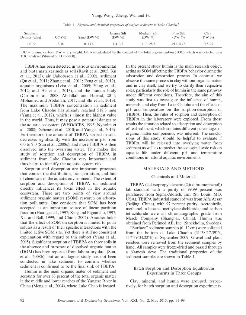
‘‘Surface’’ sediment samples (0–12 cm) were collectedfrom the bottom of Lake Chaohu (31u38917.390N,117u39934.220E) in September 2009. Gravel and plantresidues were removed from the sediment samples byhand. All samples were freeze-dried and passed througha 60-mesh sieve. The traditional properties of thesediment samples are shown in Table 1.

Batch Sorption and Desorption EquilibriumExperiments in Three Groups

Clay, mineral, and humin were grouped, respec-tively, for batch sorption and desorption experiments.

Table 1. Physical and chemical properties of surface sediment in Lake Chaohu.1

SedimentDensity (g/kg) OC (%) Sand (DW %)

Coarse Silt(DW %)

Medium Silt(DW %)

Fine Silt(DW %)

Clay(DW %)

1.1012 3.36 0–13.6 1.4–3.3 11.3–28.5 49.1–63.8 10.5–27

1OC 5 organic carbon; DW 5 dry weight. OC was calculated by the content of the total organic carbon (TOC), which was detected by aTOC analyzer (Shimadzu TOC-5000).

Yang, Wang, Zheng, Wu, and Fu


The clay group (CG) was obtained from the freeze-dried original sediment, passing through a 60-meshsieve. The mineral group (MG) was made from the claysample, with organic matter removed (Jin et al., 2008).The humin group (HG) was a mixture of 90 percentMG and 10 percent humin, which is the main organicmatter of sediment in China. Generally it occupies 63–74 percent of the total organic matter of sediment inthe middle and lower reaches of the Yangtze River(Meng et al., 2004). After treatment, the organiccarbon (OC) content of HG reached 6.74 percent.Sorption and desorption experiments were conductedby the batch equilibration technique in 1,000-mLbeakers with Teflon film caps. 0.01 M CaCl2 and NaN3

solutions were prepared for the reactor system tomaintain constant ionic strength and to inhibitmicrobial activity, respectively. The sediment samplesof CG, MG, and HG were weighed (10 g) into the glassbeaker, and 490 mL of background solution was addedto each beaker. TBBPA (0.1 g) was dissolved in 200 mLof the mixture solution with water and methanol at a10:1 (vol.:vol.) concentration to configure a 500 mg/LTBBPA stock solution. In the preparation of differentconcentrations of TBBPA the concentrations ofmethanol were controlled to lower than 0.05 percentin order to avoid the co-solvent effects. Then six levelsof initial solutions ranging from 0.1 to 10 mg/L wereadded to the beakers. After kinetic experiments12 hours was identified as the adsorption balancetime. The beakers were shaken at 150 rpm for 12 hoursat 25 6 0.5uC and centrifuged for 20 minutes at4,000 rpm. One milliliter of the supernatant and 5 gsediment were removed into the sampling vial for pre-treatment and further high-performance liquid chro-matography (HPLC) analysis. The controls containingsolutes without sediment were also conducted toevaluate TBBPA loss. Results showed that the loss ofTBBPA is less than 1 percent, which is negligible.

Desorption experiments were conducted after thecompletion of the sorption experiments, then themixtures were centrifuged. The supernatant was dis-carded. The sorbents (three groups) were washed indeionized water three times to remove surface precip-itation. After that, 500 mL of fresh background solutionwas added to the beakers, which were oscillatedcontinuously for the same period. After being shakenand centrifuged, the supernatant and sorbent sampleswere taken for pre-treatment and analysis.

Effect of pH and Temperature on Sorption andDesorption of TBBPA

The sorption and desorption experiments were alsoconducted at six different temperature points rangingfrom 4uC to 30uC and at seven pH levels, ranging

from 3 to 14 on the sediment of the CG, according tothe similar procedure used for the batch sorption-desorption experiments. Temperature was controlledin a temperature-controlled shaker. pH was adjustedwith 1 M HCI and 1 M NaOH. After being shakenand centrifuged, the supernatant and sorbent weredetermined by HPLC.

Sample Pre-treatment and Analytical Technique

The pre-treatment of supernatant samples wascarried out by the liquid-liquid extraction method.Supernatant samples were passed through a 0.45-mmmembrane filter, and 6 M HCl was used to adjust thesample to a pH of 2.0. Five hundred milliliters of thisliquid was put into a 1,000-mL tap funnel, and 15, 15,and 10 mL of CH2C12 were added at different timeintervals. After being mixed, the solution was allowedto stand until layers were formed. The CH2Cl2 liquidat the lower layer was taken. After being extracted,the liquids obtained through this method werecombined and concentrated to about 0.5 mL with arotary evaporator. The sample was dried with anitrogen blower. Methanol was added to 1 mL, andthe sample was stored at 4uC for further chromato-graphic analysis.

ASE 300 (Accelerated Solvent Extractor ASE 300,DINEX, Inc., USA) was used to execute the pre-treatment of sediment samples. The procedure is asfollows: sediment samples of three groups were putinto the extraction pool of the ASE with 34 mL ofn-hexane and methylene dichloride solvent (4:1 vol./vol.). All extracted solutions were collected, concen-trated, and purified by a bonded C18 reverse-phasesilica gel solid phase extraction column for HPLCanalysis.

TBBPA determination was performed by HPLC(Agilent 1200) using ultraviolet detection and iso-cratic elution (Sun et al., 2008c). TBBPA showedlinearity with a correlation coefficient of 0.9993,ranging from 80 to 2,000 ng/mL. The mean relativestandard deviation was less than 10.0 percent.

Data Analysis

TBBPA sorption thermodynamics were described inFreundlich and Langmuir isotherm formulas (Azizianet al., 2007; Mittal et al., 2007). The Freundlichisotherm formula was expressed as

S~Kf Ce1=n, ð1Þ

where S is the organic chemical concentration ab-sorbed by a solid substance (mg/kg); Kf and n are the

Sortion-Desorption of TBBPA


Freundlich sorption coefficients; and Ce is the equilib-rium concentration of organic matter in liquid phase atthe sorption equilibrium (mg/L).

The Langmuir isotherm formula is expressed as

Qe~KCeCmax=(1zKCe), ð2Þ

where Qe is the TBBPA concentration absorbedby sediment (mg/kg); Ce is the TBBPA equilibriumconcentration in liquid phase at sorption equilibrium(mg/L); Cmax is the maximum unit sorption quantity(mg/kg); and K is the sorption coefficient (per g).

The apparent sorption quantity Ca can be calcu-lated from the equilibrium concentration Ce and theinitial concentration C0 (mg/L) according to

Ca~(C0{Ce)V=m, ð3Þ

where V is the total volume of sorption solution (L)and m is the mass of sorbent added to the solution (g).

The standardized OC partition coefficient, KOC,can be calculated from the Kf and OC content asfollows:

KOC~Kf =OC|100: ð4Þ

The OC value of different types of sediment isobtained from Table 1 and Figure 1.

RESULTS AND DISCUSSION

Sorption and Desorption of TBBPA on the ThreeSediment Groups

The Langmuir sorption isotherms of TBBPA onthree groups of sediment are shown in Figure 1. Theorder of TBBPA equilibrium sorption quantity wasHG . CG . MG. The isotherm of MG was morenear to linear within the entire range of concentra-tions, indicating that the sorption partition of TBBPAbetween minerals and surface water had a fixedpartition coefficient. As the mineral surface had somehydroxyl groups, linear sorption may occur betweenTBBPA and the polar surfaces through hydrationfunctions (Sun et al., 2008c).

The Langmuir sorption isotherms of HG and CGwere L-type, and the sorption was unimolecular andnonlinear within the TBBPA concentrations rangingfrom 0.1 to 2.0 mg/L, but linear from 2.0 to 10.0 mg/L.It was found that CG and HG have different sorptionmodes at 2 mg/L. Solubility of TBBPA in water wasabout 2 mg/L at room temperature at pH 7.0. Whenthe TBBPA concentration was lower than 2 mg/L,sorption by CG and HG was nonlinear, but it waslinear at higher concentrations. The maximum unitsorption quantity Cmax on CG, HG, and MG was inthe range of 8.53 to 10.86 mg/kg, which was a bit lowerthan that of 24 mg/kg on fluvo-aquic soil reported bySun et al. (2008c), which was two- to threefold higherthan that of the three groups in this research. Thisdifference may be attributable to the physical andchemical properties of sediment or to a lack ofconsideration of precipitation.

TBBPA adsorption behavior also can fit a Freun-dlich model where the value of 1/n is close to 0.5. Inthe HG group it was 0.467, which was lower than 0.5(Table 2), indicating that TBBPA is easily adsorbedby the three types of sediment. The sorption capacityorder based on the 1/n value was HG . CG . MG aswell. This order is exactly consistent with the organicmatter content of the three treatment groups in

Figure 1. Sorption isotherms of TBBPA on the three groups. HGwas the humin group; OC 5 6.74 percent. CG was the clay group;OC 5 3.63 percent. MG was the mineral group.

Table 2. Fitting parameters of Freundlich and Langmuir sorption isothermal models.

Freundlich Langmuir

Kf 1/n R2 Koc Cmax (mg/kg) K R2

Clay 2.13 0.573 0.998 6,339 8.56 0.407 0.943Humin 3.65 0.467 0.996 5,415 10.86 0.642 0.941Mineral 1.47 0.622 0.968 — 8.53 0.230 0.989



descending order, for HG as 6.74 percent, and for CGas 3.36 percent.

From the adsorption results it was found thatnonlinear extent and quantities of sorption wereimproved with increasing organic matter content,while the KOC value (Table 2) between CG and HGhas only a 15 percent difference. That means thatcorrelation of KOC between sediment/soil and huminis not significant, indicating that sorption of TBBPAis related to humic acid (HA) but also to other factors(He et al., 2005). This is consistent with previousresearch (Yang et al., 2005). Related research (Sun etal., 2008b) showed that the sorption isotherms ofTBBPA on three soils were linear. However, nonlin-ear curves emerged when DOM was added to thereactor system, in which the organic matter contentwas estimated to be within the range of 6 percent to10 percent of the total sorbent. These values indicatedthat the SOM may be a predominant cause fornonlinear sorption of TBBPA in sediment.

The unit maximum sorption quantity Cmax wascalculated from the Langmuir model based on theapparent sorption quantity that did not contain theamount of precipitation. TBBPA concentrations ofthe three groups after washing with deionized waterwere also detected. The results were very differentfrom those for apparent sorption quantity. The maindifference comes from the different precipitationamount that is a part of the adsorption quantity(Javert and Heath, 1991). In this study it was physicaladsorption because it could be washed off by water.From the experimental results it was found thatwithin the TBBPA solution concentration rangingfrom 0.1 to 10.0 mg/L; the mean percentages ofTBBPA precipitation in the three groups were 69percent for MG, 45 percent for CG, and 70 percentfor HG. As shown in Figures 1 and 2, from 0.1 to1.0 mg/L of TBBPA the apparent sorption quantitiesof MG and HG were close to the sorption quantitiesin the sediment after washing; that is to say, theprecipitation was little. However, the apparentsorption quantity of CG was twofold higher thanthe mean sorption quantity after washing. Within thisrange, the order of apparent sorption quantities of thethree groups was HG . CG . MG. The order ofsorption quantities after washing precipitation onsediment was HG . MG . CG. Thus, TBBPAprecipitation quantity in CG was higher than that inthe other two groups. At 2 mg/L, TBBPA concentra-tions of HG and MG after washing suddenlydecreased, whereas that of CG increased, while theirprecipitation was higher than lower concentrations.The order of TBBPA concentrations of the threegroups after washing was CG . HG . MG, and theywere only 70 percent, 31 percent, and 37 percent of

their apparent sorption quantities, respectively. From2.0 to 10.0 mg/L, the sorption quantity of MG afterwashing increased linearly, and the mean sorption andprecipitation quantities were 33 percent and 66 percentof the apparent sorption quantity, respectively. Thesorption quantity of HG after washing reached amaximum at 5 mg/L, which was close to its apparentsorption quantity. At 10 mg/L, the sorption quantityon CG and HG after washing decreased to 18 percentand 33 percent of their apparent sorption concentra-tion, while the precipitation occupied 82 percent and67 percent, respectively.

In general, as an ionic organic compound,TBBPA’s precipitation mechanism in the three groupswas quite different from low concentration to a higherone. The sorption process of ionic organic com-pounds is closely related to their concentration ofmetal cations, which have a combining activity withionic organic compounds, leading to precipitation(Chiou, 2002). When precipitation occurs, the aque-ous calcium and sodium concentrations decrease. Sunet al. (2008c) also found that ionic strength had astrong effect on the sorption quantity of TBBPA. Theionic strengths in this study were 0.01 M CaCl2, whichmay be the predominant mechanism of TBBPAdeposited on the surface of sediments. In the analysisof adsorption of non-polar solutes on sedimentmineral, the competitive capability on mineral surfacebetween water and polar solutes is considered weakerthan that between water and non-polar solutes(Chiou, 1995, 2002). However, a significant effectbetween aqueous solution and TBBPA has occurred,and it might be attributable to the effect of cation thatcauses the shape of precipitation in this research. Inthe desorption experiments, it was significant that thedesorption ability of TBBPA was much lower than itssorption ability. The mean desorption quantities forMG, HG, and CG were 2.9 percent, 0.3 percent, and0.5 percent of the max unit sorption quantity,respectively. For each group after washing, theapparent desorption on MG was far greater thanthat on CG and HG (Figure 2). The results showedthat the TBBPA in MG was more easily desorbed.The TBBPA desorption capacities of HG and CGwere similar and were one order of magnitude lessthan the desorption quantity of MG.

Effect of pH on Sorption and Desorption of TBBPA

The CG of Lake Chaohu was selected to evaluatethe sorption law of TBBPA on surface sediment in thepH range from 3 to 14 (Figure 3). As pH increased,the sorption quantities in sediment tended to decreasegradually. Particularly at pH levels of 3 and 7, therewas a sharp decrease of sorption quantity in the



sediment. Sorption quantities at pH 3 and 7 are32.39 mg/kg and 8.56 mg/kg, respectively. Underalkaline conditions ranging from pH levels of 8 to 14,the sorption amount of TBBPA on sediment gradu-ally decreased from 7.54 mg/kg to 0.45 mg/kg.

Meanwhile, the TBBPA concentrations of the super-natants increased. The sorption quantity at pH 3 was72 times higher than that at pH 14.

In the desorption experiments, it was found thatTBBPA only has a little desorption. TBBPA concen-tration in solution increased slowly from a pH level of3 (0.012 mg/kg) and reached its highest point at a pHlevel of 14 (0.97 mg/kg). It was calculated that thepercentages of desorption quantity in the supernatantwere 0.04 percent, 0.3 percent, and 215.7 percent ofthose in the sediment at pH levels of 3, 7, and 14,respectively. Results show that the sorption quantityof TBBPA in sediment was almost equal to thedesorption quantity in supernatant at a pH 5 11.5.

TBBPA is an ionic compound with two phenolichydroxyl groups, each with two bromine atoms. ThepK1 and pK2 are 7.5 and 8.5, respectively (WHO/ICPS, 1995). It is slightly acidic and can be easilysullied and dissolved in water under alkaline condi-tions. At lower pH levels, TBBPA exists mainly in themolecular form, so physical sorption easily occurs onthe sediment surfaces with large specific surface areas.The surface of the sediment in Lake Chaohu is ahydrous oxide–type ledikite/turface surface (Jin,1995). It can attract ions from or release ions intosolution. This is mainly caused by proton dissociationand association in the exposed OH2 groups. H+

dissociation and association depends on the H+

activity in solution and the concentration of thesolution. Lower solution pH and an increasingnumber of positive charges lead to greater amountsof TBBPA absorbed through electrostatic interaction.Inversely, at higher pH, the negative charge concen-

Figure 3. The sorption-desorption of TBBPA on sediment from Lake Chaohu at different pH levels and temperatures. TBBPAconcentration (vertical axes) is the concentration of TBBPA adsorption in the sediment and the concentration of TBBPA desorption in theoverlying solution (apparent sorption quantity).

Figure 2. The percentage of precipitation, sorption quantity, anddesorption quantity of the three groups of sediment before andafter washing. The horizontal coordinates were original TBBPAconcentration levels added to the supernatant solutions. The totalprecipitation and sorption percentage after washing on the threegroups were 100 percent, respectively. DCSS was the desorptionconcentration in the supernatant. SCTW was the sorptionconcentration on the three groups after washing (parts of physicaladsorption and parts of organic matter partition). PP was theprecipitation of TBBPA on the surface of the sorbent (for thethree groups).



tration at the sediment surface is higher, and in thissituation it retains ionic TBBPA and reacts with metalcation so as to form salt or precipitation, thus sharplydecreasing the non-sorption quantity. Bisphenol Ahas analogous molecular structure and physical-chemical properties, which create similar sorptionand desorption behavior under different pH condi-tions (Zeng et al., 2006; Li et al., 2007; and Sun et al.,2008c).

Generally, the content of cations is high in naturallakes (Jin, 1995). From the results of the pH-dependent sorption and desorption procedure, it isinferred that TBBPA can form precipitation com-bined with suspended solids or sinking to the surfaceof sediment when pH is in the neutral or acidic range.For the minor desorption quantity at those situations,the TBBPA in the sediment may pose little ecologicalrisk in lakes. However, it may pose an apparentecological risk in some alkaline lakes, where pH isalways close to 10 (Jiang et al., 1988; He et al., 1996),or in a special evolution stage. For instance, the pHcan get to 8 or 9 in the period of algae bloom bursting(Cui et al., 2008; Jia et al., 2011).

Effect of Temperature on Sorption andDesorption of TBBPA

The TBBPA sorption kinetics at various tempera-tures are shown in Figure 3. As temperature increasedfrom 4uC to 30uC, the TBBPA concentration in thesupernatant gradually increased and the sorptionquantity of sediment decreased, both linearly. Therate of increase of TBBPA concentration in thesupernatant was slightly faster than that of thedecrease of sorption quantity in the sediment, whichwas 330 mg/kg-at 30uC, accounting for 9.2 percent ofthat at 4uC. As TBBPA is an ionic compound,temperature has a major influence on the sorption ofpolar organic compounds by the sediment, andsorption should be a process of heat release, asincreased temperature both improves solubility inwater and decreases sorption on the sediment (Chiou,2002). Desorption of TBBPA on the sediment atdifferent temperatures is shown in Figure 3. Thesorption quantity on sediment rapidly decreased withincreasing temperature, whereas that of the superna-tant slowly increased. The desorption quantity at 4uCwas 11.1 percent of that at 30uC, where it was almostequal to the sorption quantity on sediment. Ingeneral, the water solubility of organic compoundscould be improved with the rising temperature, yet itssorption quantity would be decreased (Liu and Ji,1996). Being an exothermic process, the sorptionquantity keeps decreasing with decreasing tempera-ture (Kozak et al., 1983).

CONCLUSION

Sorption and desorption behaviors of TBBPA inthree types of sediment were investigated in this study.The results show that the Freundlich model candescribe the sorption behavior of TBBPA well. Themagnitude of the sorption capability was as follows:HG . CG . MG. Desorption capability of the sortwas the opposite. It was found that precipitationsorption was the main sorption type of TBBPA onsediment. Its percentage ranged from 45 percent to 70percent of the total sorption. In sorption-desorptionexperiments on clay sediment it was indicated that thesorption of TBBPA decreased with increasing solutionpH and temperature, ranging from 3 to 14 and 4uC to30uC, respectively. Moreover, sorption and desorptionreached a dynamic equilibrium at a pH level of 11.5and at a temperature of 30uC, respectively. This showsthat the release of TBBPA from the sediment is higherin summer than in the other three seasons in LakeChaohu. The results provide a better understanding ofthe transportation and potential ecological risk ofTBBPA for aquatic life in lakes.

ACKNOWLEDGMENTS

This study was financially supported by the StateMajor Water Project (SMWP, 2012zx07503-003). Theauthors thank the SMWP as well as the members ofthe project steering group. We also thank threeanonymous reviewers for reviewing the manuscriptand for their helpful comments.

REFERENCES

ABDALLAH, M. A.; AND HARRAD, S., 2011, Tetrabromobisphenol-A, hexabromocyclododecane and its degradation products inUK human milk: Relationship to external exposure: Envi-ronment International, Vol. 37, No. 2, pp. 443–448.

AZIZIAN, S.; HAERIFAR, M.; AND BASIRI-PARSA, J., 2007, Extendedgeometric method: A simple approach to derive adsorptionrate constants of Langmuir–Freundlich kinetics: Chemo-sphere, Vol. 68, No. 11, pp. 2040–2046.

CARIOU, R.; ANTIGNAC, J. P.; ZALKO, D.; BERREBI, A.; CRAVEDI,J. P.; MAUME, D.; MARCHAND, P.; MONTEAU, F.; RIU, A.;ANDRE, F.; AND LE BIZEC, B., 2008, Exposure assessment ofFrench women and their newborns to tetrabromobisphenol-A: Occurrence measurements in maternal adipose tissue,serum, breast milk and cord serum: Chemosphere, Vol. 73,No. 7, pp. 1036–1041.

CHIOU, C. T., 1995, Comment on: ‘Thermodynamics of organicchemical partition in soils’: Environmental Science Technol-ogy, Vol. 29, No. 5, pp. 1421–1423.

CHIOU, C. T., 2002, Partition and Adsorption of OrganicContaminants in Environmental Systems: Wiley-Interscience,Hoboken, NJ. 213 p.

CUI, F.; HUANG, Z.; LIU, Z.; AND FU, M., 2008, Relationship amongchlorophyll a, dissolved oxygen and pH in the period of algaebloom: Waste Water Engineering, Vol. 34, pp. 177–178.



DARNERUD, P. O., 2003, Toxic effects of brominated flame

retardants in man and in wildlife: Environment International,

Vol. 29, No. 6, pp. 841–853.

DEBENEST, T.; GAGNE, F.; PETIT, A. N.; ANDRE, C.; KOHLI, M.; AND

BLAISE, C., 2010, Ecotoxicity of a brominated flame retardant

(tetrabromobisphenol A) and its derivatives to aquatic

organisms: Comparative Biochemistry Physiology Part C:

Toxicology Pharmacology, Vol. 152, No. 4, pp. 407–412.

FENG, A. H.; CHEN, S. J.; CHEN, M. Y.; HE, M. J.; LUO, X. J.; AND

MAI, B. X., 2012, Hexabromocyclododecane (HBCD) andtetrabromobisphenol A (TBBPA) in riverine and estuarine

sediments of the Pearl River Delta in southern China, with

emphasis on spatial variability in diastereoisomer- and

enantiomer-specific distribution of HBCD: Marine Pollution

Bulletin, Vol. 64, No. 5, pp. 919–925.

HE, M. C.; DENG, H. Z.; LI, X. R.; AND YING, Y., 2005, Sorptionof phenanthrene by humic acids from different soils: Journal

Environmental Sciences, Vol. 25, No. 7, pp. 982–988.

HE, M. J.; LUO, X. J.; YU, L. H.; WU, J. P.; CHEN, S. J.; AND MAI,

B. X., 2013, Diasteroisomer and enantiomer-specific profiles

of hexabromocyclododecane and tetrabromobisphenol A in

an aquatic environment in a highly industrialized area, SouthChina: Vertical profile, phase partition, and bioaccumula-

tion: Environmental Pollution, Vol. 179, pp. 105–110.

HE, Z.; JIANG, H.; AND BI, F., 1996, Restudies on the

hydrochemistry and hydrobiology of Dali Lake: Journal

Dalian Fish College, Vol. 11, No. 2, pp. 1–13. (In Chinese.)

HUANG, W.; YOUNG, T.; SCHLAUTMAN, M. A.; YU, H.; AND WEBER,

W. J., Jr., 1997, A distributed reactivity model for sorption

by soils and sediments. 9. General isotherm nonlinearity and

applicability of the dual reactive Domin model: Environmen-

tal Science Technology, Vol. 31, No. 6, pp. 1703–1710.

JAKOBSSON, K.; THURESSON, K.; RYLANDER, L.; SJODIN, A.;HAGMAR, L.; AND BERGMAN, A., 2002, Exposure to poly-

brominated diphenyl ethers and tetrabromobisphenol A

among computer technicians: Chemosphere, Vol. 46, No. 5,

pp. 709–716.

JANER, G.; HAKKERT, B. C.; SLOB, W.; VERMEIRE, T.; AND PIERSMA,A. H., 2007, A retrospective analysis of the two-generation

study: What is the added value of the second generation?:

Reproductive Toxicology, Vol. 24, No. 1, pp. 97–102.

JAVERT, C. T. AND HEATH, J. K., 1991, Sediment- and saturated-soil-

associated reactions involving an anionic surfactant (dodecyl-

sulfate). 1. Precipitation and Micelle Formation: Environmen-

tal Science Technology, Vol. 25, No. 6, pp. 1031–1038.

JIA, X.; SHI, D.; SHI, M.; LI, R.; SONG, L.; FANG, H.; YU, G.; LI, X.;

AND DU, G., 2011, Formation of cyanobacterial blooms in Lake

Chaohu and the photosynthesis of dominant species hypothesis:

Acta Ecology Sinica, Vol. 31, No. 11, pp. 2969–2977.

JIANG, D.; ZHAI, P.; MA, P.; DUAN, R.; YANG, Y.; AND CHEN, Y.,

1988, Changes of contains for elements in water and sediment

of Chenghai, a lake of Yunnan Plateau, in dry and rainy

seasons and group of actinomycetes in it: Journal Yunnan

University, Vol. 10, No. 2, pp. 153–159.

JIN, X., 1995, Lake in China Research of their Environment: ChinaOcean Press, Beijing, China, 318 p.

JIN, X.; WANG, S.; ZHAO, H.; ZHOU, X.; AND WU, F., 2008, Effect

of organic matter on DOM sorption on lake sediments:

Environment Geology, Vol. 56, No. 2, pp. 391–398.

JOHNSON-RESTREPO, B.; ADAMS, D. H.; AND KANNAN, K., 2008,Tetrabromobisphenol A (TBBPA) and hexabromocyclodo-

decanes (HBCDs) in tissues of humans, dolphins, and sharks

from the United States: Chemosphere, Vol. 70, No. 11,

pp. 1935–1944.

KOZAK, J.; WEBER, J. B.; AND SHEETS, T. J., 1983, Adsorption ofprometryn and metolachlor by selected soil organic matterfractions: Soil Sciences, Vol. 136, No. 2, pp. 93–101.

LEIST, T. G.; POTTER, D.; HEBERT, C. E.; AND LETCHER, R. J., 2009,Temporal trends and spatial distribution of non-polybromi-nated diphenyl ether flame retardants in the eggs of colonialpopulations of Great Lakes herring gulls: EnvironmentalScience Technology, Vol. 43, No. 2, pp. 312–317.

LI, J.; ZHOU, B.; SHAO, J.; YANG, Q.; LIU, Y.; AND CAI, W., 2007,Influence of the presence of heavy metals and surface-activecompounds on the sorption of bisphenol A to sediment:Chemosphere, Vol. 68, No. 7, pp. 1298–1303.

LI, Y. N. AND ZHOU, Q. X., 2008, Metabolic transformation andecotoxicology of tetrabromobisphenol A: A review: JournalEcology, Vol. 27, pp. 263–268. (In Chinese.)

LIU, W. P. AND JI, J., 1996, Sorption and desorption—the keyfactor of pesticides fate in soil-water environment: ChinaEnvironmental Sciences, Vol. 16, No. 1, pp. 25–30.

MENG, F. D.; JIANG, X.; AND JIN, X. C., 2004, Physical-chemicalcharacteristics of the sediments in lakes from the middle andlower reaches of the Yangtze River: Research EnvironmentalSciences, Vol. 17, pp. 24–29.

MITTAL, A.; KURUP, L.; AND MITTAL, J., 2007, Freundlich andLangmuir adsorption isotherms and kinetics for the removalof tartrazine from aqueous solutions using hen feathers:Journal Hazardous Material, Vol. 146, pp. 243–248.

MOHAMED, A. E. AND ABDALLAH, S. H., 2011, Tetrabromobisphenol-A, hexabromocyclododecane and its degradation products inUK human milk: Relationship to external exposure: Environ-ment International, Vol. 37, No. 2, pp. 443–448.

MORRIS, S.; ALLCHIIN, C. R.; ZEGERS, B. N.; HAFTKA, J. J. H.;BOON, J. P.; BELPAIRE, C.; LEONARDS, P. E. G.; VAN LEEUWEN,S. P. J.; AND DE BOER, J., 2004, Distribution and fate ofHBCD and TBBPA brominated flame retardants in NorthSea estuaries and aquatic food webs: Environmental ScienceTechnology, Vol. 38, No. 21, pp. 5497–5504.

NYHOLM, R. J.; ANNA, N.; LEIF, N.; PETER, H.; AND PATRIK, L. A.,2008, Maternal transfer of brominated flame retardants inzebrafish (Danio rerio): Chemosphere, Vol. 73, pp. 203–208.

QU, G. B.; SHI, J. B.; WANG, T.; FU, J.; LI, Z.; WANG, P.; RUAN, T.;AND JIANG, G., 2011, Identification of tetrabromobisphenol Adiallyl ether as an emerging neurotoxicant in environmentalsamples by bioassay-directed fractionation and HPLC-APCI-MS/MS: Environmental Science Technology, Vol. 45, No. 11,pp. 5009–5016.

RAVIT, B.; EHRENFELD, J. G.; AND HAGGBLOM, M. M., 2005, Saltmarsh rhizosphere affects microbial biotransformation of thewidespread halogenated contaminant tetrabromobisphenol-A(TBBPA): Soil Biology Biochemistry, Vol. 37, No. 6, pp. 1049–1057.

SHI, Z. X.; JIAO, Y.; HU, Y.; SUN, Z. W.; ZHOU, X. Q.; FENG, J. F.;LI, J. G.; AND WU, Y. N., 2013, Levels of tetrabromobi-sphenol A, hexabromocyclododecanes and polybrominateddiphenyl ethers in human milk from the general population inBeijing, China: Science Total Environment, Vol. 452–453,pp. 10–18.

SHI, Z. X.; WU, Y. N.; LI, J. G.; ZHAO, Y. F.; AND FENG, J. F.,2009, Dietary exposure assessment of Chinese adults andnursing infants to tetrabromobisphenol A and hexabromocy-clododecanes: Occurrence measurements in foods and humanmilk: Environmental Science Technology, Vol. 43, pp. 4314–4319.

SUN, Z.; MAO, L.; FENG, Z.; YU, Y.; FENG, J.; AND YU, H., 2008a,Sorption and desorption behaviours of tetrabromobisphenolA on fluvo-aquic soil: Environmental Sciences, Vol. 29, No. 10,pp. 2874–2878. (In Chinese.)



SUN, Z.; MAO, L.; FENG, Z.; YU, Y.; AND YU, H., 2008b, Effects ofhumic acid on sorption of tetrabromobisphenol A by soils:China Environmental Sciences, Vol. 28, No. 8, pp. 748–752.

SUN, Z. H.; YU, Y. J.; MAO, L.; ZHENG, F.; AND YU, H. X., 2008c,Sorption behaviour of tetrabromobisphenol A in two soilswith different characteristics: Journal Hazardous Material,Vol. 160, pp. 450–461.

VELDHOEN, N.; BOGGS, A.; WALZAK, K.; AND HELBING, C. C., 2006,Exposure to tetrabromobisphenol-A alters TH-associated geneexpression and tadpole metamorphosis in the Pacific tree frogPseudacris regilla: Aquatic Toxicology, Vol. 78, pp. 292–302.

WHO/ICPS, 1995, Environmental Health Criteria 172. Tetrabro-mobisphenol A and Derivatives: World Health Organization,Geneva, Switzerland, 12–38 p.

XIA, G. AND BALL, W. P., 1999, Adsorption-partitioning uptake ofnine low-polarity organic chemicals on a natural sorbent:Environmental Science Technology, Vol. 33, No. 2, pp. 262–269.

XING, B. AND PIGNATELLO, J. J., 1997, Dual-mode sorption of lowpolarity compounds in glassy poly(vinylchloride) and soilorganic matter: Environmental Science Technology, Vol. 31,No. 3, pp. 792–796.

XU, J.; GAO, Z. S.; XIAN, Q. M.; YU, H. X.; AND FENG, J. F., 2009,Levels and distribution of polybrominated diphenyl ethers(PBDEs) in the freshwater environment surrounding a PBDEmanufacturing plant in China: Environmental Pollution,Vol. 157, pp. 1911–1916.

XU, T.; WANG, J.; LIU, S. Z.; LU, C.; SHELVER, W. L.; LI, Q.X.; AND LI, J., 2012, A highly sensitive and selectiveimmunoassay for the detection of tetrabromobisphenol Ain soil and sediment: Analytica Chimica Acta, Vol. 751,pp. 119–127.

YANG, K.; ZHU, L.; LOU, B.; AND CHEN, B., 2005, Correlationsof nonlinear sorption of organic solutes with soil/sedimentphysicochemical properties: Chemosphere, Vol. 61, No. 1,pp. 116–128.

YANG, S. W.; WANG, S. R.; WU, F. C.; YAN, Z. G.; AND LIU, H. L.,2012, Tetrabromobisphenol A: tissue distribution in fish,and seasonal variation in water and sediment of LakeChaohu: Environmental Sciences Pollution Research, Vol. 19,pp. 4090–4096.

YANG, S. W.; XU, F. F.; ZHENG, B. H.; AND WU, F. C., 2013,Multibiomarker responses upon exposure to tetrabromobi-sphenol A in the freshwater fish Carassius auratus: AquaticToxicology, Vol. 142–143, pp. 248–256.

ZENG, G.; ZHANG, C.; HUANG, G.; YU, J.; WANG, Q.; LI, J.; XI, B.;AND LIU, H., 2006, Adsorption behavior of bisphenol A onsediment in Xiangjiang River, Central-south China: Chemo-sphere, Vol. 65, No. 9, pp. 1490–1499.

ZHANG, P.; LI, Y.; LI, J.; AND LI, Y., 2011, Exposure anddistribution of TBBPA in the water and sediments from LakeChaohu: Inner Mongolia Science Technology Economy, Vol. 5,pp. 51–55. (In Chinese)



Gully Erosion Mapping Using Object-Based and

Pixel-Based Image Classification Methods

AYOOB KARAMI

Faculty of Natural Resources, Hormozgan University, Minab Road, Bandar Bbbas,Hormozgan Province, P.O. Box 3995, Iran

ASADOLLAH KHOORANI1

Faculty of Natural Resources, Hormozgan University, Minab Road, Bandar Bbbas,Hormozgan Province, P.O. Box 3995, Iran

AHMAD NOOHEGAR

Faculty of Natural Resources, Tehran University, Karaj, Iran

SEYED RASHID FALLAH SHAMSI

College of Agriculture, Shiraz University, Shiraz Province, P.O. Box 71454, Iran

VAHID MOOSAVI

Faculty of Natural Resources, Yazd University, Yzad Province, Iran

Key Terms: Gully Erosion, Object-Based Classifica-tion, Digital Mapping, IRS-P6, Iran

ABSTRACT

Gully erosion mapping is a crucial step to monitorthe erosion process and to study its current and futurelocal impacts. Gully erosion mapping through field-work is difficult, time-consuming, and costly. Thisarticle compares various pixel-based image classifica-tion (PBC) algorithms, such as ISODATA, MaximumLikelihood Classification, and Support Vector Ma-chine, with the object-based image analysis (OBIA)technique for gully erosion mapping on IRS-P6 images.Six models defined by classification types, classifiers,and feature spaces were built for comparison. Theresults show that OBIA classification performed betterthan PBC in terms of accuracy. We also found that theimprovement of OBIA was primarily due to employingtextural and shape features and optimized featurespace, while the use of standard feature space did notimprove OBIA. In addition, OBIA significantly re-duced the salt-and-pepper effect that obscures thefeatures on the output maps compared to the PBCmaps (which had more salt-and-pepper effects). Itseems that object-based techniques have yielded betterresults because of their focus on the shape of gully

networks rather than on their spectral heterogeneity. Inorder to improve the accuracy, a priority may be gainedby fully exploring the use of membership function andhierarchical approach with multi-scale segmentation forgully mapping. In future studies we propose todetermine how these factors can affect the performanceof OBIA in terms of gully mapping. This study providesinformation on the location of gullies, gully dynamicsover a period of time, and the degree of landdegradation (gully density) for developing and imple-menting soil conservation measures.

INTRODUCTION

Gullies in the Fars Province of Iran are large anddeep natural ditches or channels in a landscapeformed by running water. Recent studies reveal thatgully erosion is often a main source of sedimentproduction (Valentin et al., 2005) and can vary tobetween 10 percent and 94 percent of total sedimentyield caused by water erosion (Poesen et al., 2003).Gully erosion causes adverse environmental impactsand high economic costs by negatively affectingagricultural production, water quality, and facilities(Valentin et al., 2005; Taruvinga, 2008). Gully erosiongenerally is considered as an indicator of desertifica-tion and land degradation (UNEP, 1994). Hence,detailed identification and monitoring and mappingof gully development over time are essential require-ments for estimating sediment production, soil1Corresponding author email: [email protected].


conservation measures, and identification of vulner-able areas for gully formation, land degradation, andenvironmental impacts (Shruthi et al., 2011).

Gully erosion mapping is a time-consuming,difficult job when fieldwork is used alone. Aerialphoto visual interpretation is also time-consumingand costly and is limited by the interpreter skills(Vrieling, 2007; Taruvinga, 2008; and Shruthi et al.,2011). Nowadays an alternative for this type of visualinterpretation technique is the automatic extractionof gully erosion from satellite imagery. The remotesensing approach is the only practical method formapping gully features because of the large area andcomplexity of the size, shape, and occurrence of thegully features (Knight et al., 2007).

Automatic soil erosion mapping using remotesensing techniques was initiated by pixel-based orper-pixel image classification (PBC), which only usesthe surface reflectance values contained in pixels(Shruthi et al., 2011). PBC uses multi-spectralclassification techniques to assign a pixel to a classconsidering only the spectral similarities with aclass. Various PBC methods, such as MaximumLikelihood Classification (MLC), Mahalanobis dis-tance classifier, and Support Vector Machine (SVM),are employed for thematic mapping and quantitativeanalysis of gully erosion (Valentin et al., 2005;Taruvinga, 2008).

Gullies are complex features to map since theirspectral heterogeneity is associated with the presenceof bare soil, vegetation, or shadow- or moisture-related brightness differences (Taruvinga, 2008;Shruthi et al., 2011). The spectral heterogeneity ofgullies themselves causes their spectral similarity toother land covers, tending to produce ‘‘speckled’’ or‘‘salt-and-pepper’’ image classification results (Tzot-sos et al., 2008; Whiteside et al., 2011). In addition,previous studies have shown that PBC techniquessuch as MLC and SVM algorithms could not separatewater erosion features at an acceptable level ofaccuracy as a result of the spectral similarities withother non-erosion features (Solaimani and HadianAmri, 2008; Taruvinga, 2008; Pirie, 2009; Torkash-vand and Alipour, 2009; Shruthi et al., 2011; andMararakanye and Nethengwe, 2012).

Gully erosion features have shape, length, topolog-ical entities, and textural characteristics that make itpossible to treat them as spatial objects that can becharacterized based not only on their geometricproperties but also on their spatial relationship withsurrounding features. A review of the literatureindicates that the potential for gully erosion mappingusing object-based image analysis (OBIA) fromspace-borne imagery has not been thoroughly ex-plored. Since gullies have both measurable geometric

and spatial properties, object analysis, as opposed toindividual pixels, may be more appropriate to addressthe spectral ambiguity problems and may be moresuitable for knowledge-driven analysis (similar tovisual image interpretation).

Some investigations in gully erosion mapping byOBIA have already been performed (Shruthi et al.,2011). Knight et al. (2007) used ASTER imagery tomap alluvial gullies associated with large tropicalrivers in Australia, while Eustace et al. (2009) usedhigh-resolution LiDAR data to successfully mapgully extent and density using OBIA. Shruthi et al.(2011) investigated the use of OBIA to extract gullyerosion features from IKONOS and GEOEYE-1 datausing a combination of topographic, spectral, shape(geometric), and contextual information.

Mararakanye and Nethengwe (2012) investigatedand tested the OBIA technique for gully featureidentification in the Limpopo Province in SouthAfrica. Knight et al. (2007) gained approximately 50percent accuracies for the gully class, showing that anobject-based approach does not automatically lead tosuperior results. Shruthi et al. (2011) found thatOBIA gully mapping is quicker and more objectivethan traditional image-digitization methods. Basedon previous studies (e.g., Baatz and Schape, 2000;Platt and Rapoza, 2008), factors such as texture andshape, membership function, and hierarchical ap-proach with multi-scale segmentation are importantto include in the analysis to improve the accuracy andefficiency of OBIA.

This study represents the first attempt to conduct adetailed comparison of OBIA and PBC for mappinggullies in Lamerd, Fars Province, Iran, using medium-resolution IRS-P6 data. Accuracies for the classifica-tions are produced and compared using statisticaltests.

STUDY AREA AND RESEARCH DATA

The study area (14 3 11 km) is located in LamerdTownship, Fars Province, in the southwestern regionof Iran (Figure 1). The study area has an arid climate,with nine clear, dry seasons and an average annualrainfall of 250 mm. The rainy season is fromDecember to March, with highest amount andintensities of rain occurring in the month of February.The terrain is flat, with slopes measuring between 0percent and 2 percent and with elevations rangingfrom 389 m to 2,165 m (most ranging between 400and 600 m). Most soils (texture) in the area consist ofclay loam that are generally saline soil. The range ofelevation, mean annual precipitation and tempera-ture, geological formation, land use, landform, and

Karami, Khoorani, Noohegar, Shamsi, and Moosavi


climate type and soil order are included in Table 1.Gully erosion is the most significant erosion feature inthe area, with gullies measuring as deep as 2.5 m andabout 10 m wide. The gullies are U-shaped anddendritic (Figure 2).

The Data

A multi-spectral data set of Indian Remote Sensingsatellite (IRS-P6), dated August 2008, have been usedin this research, and include blue, green, red, and NIRbands of 23.5 m and a Panchromatic band of 5.8 m.The imagery was radiometrically and geometricallycorrected and rectified to the world geodetic survey1984 datum (WGS84) and the Universal Transverse

Figure 1. Study area situated over the southwestern region of Fars Province (Fars, Iran). (a) Location. (b) IRS-P6 data showing thegully networks.

Table 1. General characteristics of the study area (after fromKompani-Zare et al., 2011).

Name Lamerd

Mean elevation (m) 400Mean annual precipitationa (mm) 250Mean annual temperature (uC) 24Geology QuaternaryLand use Farming-poor rangeLandform type Flood plainClimate typec BWh, BShSoil orders Aridsols, Entisols

aBased on Lamerd Station, 1993 to 2010.bPoor range: the range land with mean coverage of less than 20percent.cBWh 5 arid-desert-hot arid; BSh 5 arid-steppe-hot arid.

Gully Erosion Mapping


Mercator coordinate system. Image-to-map registra-tion using a second-order polynomial transformationled to a 0.3-pixel root mean square error for multi-spectral imagery and an 0.5-pixel error for panchro-matic imagery. A visual assessment confirmed that allimage sources were aligned with ancillary data layersof higher spatial accuracy (e.g., road network anddrainage network).

Radiometric processing was applied to the satelliteimagery. Absolute atmospheric correction of theimagery was not performed because of the lack of

simultaneously acquired ground-based spectral dataor appropriate meteorological data available in thestudy area. Instead, a relative correction using theDark-Object Subtraction method was used to reducethe atmospheric scattering effects (Chavez, 1988).

Training/Test Data Set and Field Works

A commonly accepted practice for assessing productsderived from coarse resolution data using semi-auto-matic classification techniques is the use of a higher

Figure 2. Gullies in the Lamerd region (southwestern region of Iran). (a) U-shaped gully. (b, c) Presence of dry and alive vegetation ingullies. (d) Dendritic gully system on IRS-P6 data.

Figure 3. Procedure of ground truth map preparation.



resolution satellite data as a reference (Taruvinga, 2008).‘‘Ground truth’’ maps that have gully and non-gullyclasses were created using traditional gully mappingmethods on the IRS-P6 panchromatic image subset andGoogle Earth images, as summarized in Figure 3. Theground truth map was produce during an intensivefield validation effort to check and confirm the existinggully erosion map. In this research two training datasets were used, presenting the gullies and non-gullies,confirmed through field checks and delineated as apolygonal training area on screen.

METHODS

Image Classification

In addition to the original IRS-P6 bands, four setsof test data were generated using ENVI software(ENVI, 2008) in order to evaluate the impact ofincluding additional bands in ISODATA and MLCclassifications. In the first set, only the original bandsof green, red, NIR, and SWIR were used (Set 1 5 B1,B2, B3, B4). In the second set, the first principlecomponent (PC1) was added to the original bands(Set 2 5 B1, B2, B3, B4, BPCA1). In the third data set,the PC2 was included in the original bands (Set 3 5

B1, B2, B3, B4, BPCA2). Finally, in the fourth data set,both PCs were included in the original data set (Set 45 B1, B2, B3, B4, BPCA1, BPCA2).

To evaluate the performance of OBIA and PBCtechniques, a set of image classification models(Table 2) was constructed. The models are construct-ed through a multiple comparison procedure. All fourdata sets (Sets 1, 2, 3, and 4) were classified using

ISODATA and MLC models, and then the data setthat produced the highest accuracy was selected forSVM and OBIA. The PBC classification models(models 1, 2, and 3) were conducted using ENVI 4.3,while others were conducted using eCognition pack-age (Definiens, 2004).

PBC

The PBC was performed using the ISODATA,MLC, and SVM algorithms. The ISODATA algo-rithm is the most frequently and widely usedunsupervised classifier, and it was used in model 1to test the traditional unsupervised PBC. The imagerywas initially classified into four classes with maximumiterations of five and a convergence threshold of 0.95,after which it was coded into two classes.

MLC is one of the most powerful and frequentlyused parametric supervised PBC methods (Huanget al., 2002; Yan et al., 2006; Qian et al., 2007; Dixonand Candade, 2008; Kavzoglu and Colkesen, 2009;Otukei and Blaschke, 2010; and Ouyang et al., 2011),and it was used in model 2. The MLC calculates astatistical (Bayesian) probability function from theinputs for classes established from training sites. Eachpixel is then assigned to the class to which it mostlikely belongs.

SVM is a group of theoretically superior machinelearning algorithms and one of the latest additions tothe existing catalog of image classification techniquesthat support gully mapping (Taruvinga, 2008). Essen-tially, SVM is based on fitting a separating hyper-planethat provides the best separation between two classesin a multidimensional feature space. In order torepresent more complex shapes than linear hyper-planes, a variety of kernels, including the linear,polynomial, the radial basis function (RBF), and thesigmoid, can be used (Petropoulos et al., 2012).

In addition, a penalty parameter can be introducedto the SVM classifier to allow form in classificationduring the training process. The input parametersrequired for running SVMs in ENVI include thegamma (c) in the kernel function, the penaltyparameter, the number of pyramid levels to use, andthe classification probability threshold value. Verylittle guidance exists in the literature concerning thecriteria to be used in selecting the kernel-specificparameters (e.g., Carrao et al., 2008; Li and Liu,2010).

The c parameter was set to a value equal to theinverse of the number of the spectral bands of theimagery, whereas the penalty parameter was set to itsmaximum value (i.e., 100), forcing no misclassifica-tion during the training process. The pyramid

Table 2. Classification models built for PBC and OBIA comparison.

Model Classifier Data SetFeatureSpace

1 PBC ISODATA Set 1 SFSSet 2 SFSSet 3 SFSSet 4 SFS

2 PBC MLC Set 1 SFSSet 2 SFSSet 3 SFSSet 4 SFS

3 PBC SVM—RBF Set 4 SFSSVM—liner Set 4 SFSSVM—polynomial Set 4 SFSSVM—sigmoid Set 4 SFS

4 PBC NN Set 4 SFS5 OBIA NN Set 4 SFS6 NN Set 4 OFS

NN 5 nearest neighbor; MLC 5 maximum likelihood; SFS 5

standard feature space; OFS: 5 optimized feature space; Set 1 5

B1, B2, B3, B4; Set 2 5 B1, B2, B3, B4, BPCA1; Set 3 5 B1, B2, B3,B4, BPCA2; Set 4 5 B1, B2, B3, B4, BPCA1, BPCA2.



parameter was set to a value of zero, whereas aclassification probability threshold of zero was used,meaning that all image pixels had to be classified intoone class.

OBIA

In the OBIA, the basic processing units are imageobjects or segments, not single pixels (Dehvari andHeck, 2009). There are unique advantages to OBIA.Multi-scale approaches are one advantage, and thepossibility of using geometric or contextual featuresin both segmentation and classification is another.

The segments are regions (groups of pixels) that aregenerated by one or more criteria of homogeneity.The segmentation algorithm used in eCognitionsoftware is a bottom-up region merging algorithmthat begins with 1-pixel objects. The procedureincludes a pairwise clustering process to mergesmaller objects into larger ones with uniform textureand color, as well as an optimization process definedby a set of parameters, such as scale, color, and shape.When the spectral and spatial heterogeneity of oneobject reaches a defined threshold, the procedurestops its growth. The size of an image object(segment) is determined by a scale parameter (adimensionless integer). A larger scale parametercauses larger image segments (Aksoy and Ercanoglu,2011).

Two other optimization parameters, color (color 5

1-shape) and shape values, weighted from 0 to 1, arethe other important parameters in segmentation. Thecolor value refers to the spectral homogeneity and isvery important for creating meaningful objects. Theshape criterion defines the textural homogeneity ofthe resulting image objects, and it is divided into twogroups, such as smoothness and compactness. Thesmoothness criterion is used to optimize image objectswith regard to smoothness of borders, while thecompactness criterion is used to optimize imageobjects with regard to compactness.

Image segmentation is the first step in OBIA.Different groups of possible parameters were tested to

identify a good scale comparing segmented objectswith uniform visual properties of the imagery. Afterseveral trial-and-error attempts to find the appropri-ate multi-resolution segmentation parameters, theselected values were determined to be 60, 0.8, 0.2,0.4, and 0.6 for scale, color, shape, smoothness, andcompactness, respectively (Table 3). The segmenta-tion parameters used to provide optimal classificationresults are shown in Table 3.

A nearest neighbor classifier (NN) was alsoadopted to conduct supervised classification in dataset 4 (models 5 and 6). The NN classifies each imageobject into the class that has the sample object closestto it in a given feature space (Baatz et al., 2004). Aftersegmenting the images the OBIA variables wereselected. The object features allow for contextualrelationships between image objects to be incorpo-rated into the OBIA.

Feature Spaces

Different feature spaces were explored in order totest the influence of texture and shape features onclassification. Typically in PBC methods, the imageclassification algorithm employs standard featurespace (SFS) comprising blue, green, red, and near-infrared bands. Nevertheless, classification sometimesalso takes advantage of features other than standardspectral features. This is especially important for theOBIA, as objects represent more features than pixels.Features of objects include spectrum, shape, texture,and context, while features of pixels are limited tospectrum and texture.

To evaluate the effect of shape and texture featureson classification, optimized feature space (OFS) andSFS were compared. The optimized features wereobtained from the feature space optimization proce-dure, which calculates a subset of feature space withthe greatest separate distance at a given dimension(Baatz et al., 2004). The optimized feature space ofthe OBIA (model 6) is listed in Table 4.

Table 3. Parameter value used in multi-resolution segmentationalgorithm.

Image Segmentation Parametersa

Scale Color/Shape Smoothness/Compactness

20 0.6/0.4 0.7/0.330 0.5/0.5 0.6/0.460 0.8/0.2 0.4/0.6

aImage layers used: B1, B2, B3, B4, Bpca1, Bpca2.

Table 4. Feature bands composition of the optimized space.

Feature Descriptions

Mean layer value The overall brightness of all bandsWidth Main width of the objectLength:width ratio The ratio of main length to main width

of objectsDistance to line Distance to line that shows the main

gully’s directionAverage area Average area represented by segmentsStandard deviation Standard deviation area represented by

segments



Accuracy Assessment

In order to assess the classification accuracy of themodels, the error matrices were established to make acomparison between the classification results and thetruth. The class attributes of points on the groundtruth map were compared to those on the classifiedimage for each model. Thus, 15 matrices wereestablished, and the heuristics are shown in Table 5.

The McNemar’s test has been employed for paired-sample nominal scale data to assess whether statisti-cally significant differences exist between the classifi-cation results (Foody, 2004; Whiteside et al., 2011;and Duro et al., 2012). This non-parametric test thatis based on a chi-square (x2) statistics (Eq. 1) was usedto assess whether there is a statistically significantdifference between the PBC and the OBIA results.

x2~( f12{f21)2

f12zf21ð1Þ

where f12 represents the number of the pixels,incorrectly classified by the first classifier, whilecorrectly classified by the second classifier; and f21

represents the number of the pixels, correctlyclassified by the first classifier, incorrectly classifiedby the second classifier (Foody, 2004; Petropoulouset al., 2012).

RESULTS

Overall accuracy and kappa coefficients of themodels ranged from 54 percent to 90 percent andfrom 0.15 to 0.82, respectively (Table 5). The OBIAmodel 6 reached an overall accuracy of 89.6 percentand a kappa coefficient of 0.82, which was the highestamong all models. The most accurate PBC model was

supervised model 2, which had an overall accuracy(82 percent) and kappa coefficient (0.62) but wassignificantly lower than that of model 6.

In addition, Figure 4 shows that an OBIA modelsignificantly reduced the salt-and-pepper effect whencompared to the PBC models (models 2 and 3). In thiscase, OBIA was superior to PBC in terms ofextracting ground objects, showing more accuracyin classification, and was more noticeable in shapes.These results are consistent with those of other studiesconcerning the comparison between OBIA and PBC(Qian et al, 2007; Dehvari and Heck, 2009; Ouyanget al., 2011; and Duro et al., 2012) (Figure 4).

PBC

Models 1 and 2 were compared, and the algo-rithm’s performances were tested. Additional bandsof the original data were also evaluated. The resultsare given in Table 5 and show that the calculatedkappa coefficients are different between the twoalgorithms of four different data sets (Sets 1, 2, 3and 4). Model 2, with data set 4, has a kappacoefficient of 0.62 and an overall accuracy of 82percent, which was the highest achieved. When theclassification methods were considered, the patternsobserved Figure 4 indicate that model 2 (MLC)generally provided a superior result to that of model1 (ISODATA).

When the data sets were considered, it was evidentfrom Table 5 that substantial improvements wereachieved when model 2 was developed by addingmore variables instead of using only four bands.There were significant differences in the accuracyvalues when PCA1 and PCA2 bands were added,respectively, to model 2. However, there were minordifferences in the accuracy values when PCA bandswere added to model 1.

The output maps that provided the highestaccuracy result obtained from the data sets formodels 1 and 2 were also compared using the model3 accuracy assessment. The classification accuracyassessment results produced from models 2 and 3 fordata set 4 are shown in Table 5. For model 3 (i.e.,SVMs), higher accuracy was produced from the SVMwith sigmoid kernel, which showed an overallaccuracy of 80 percent and a kappa coefficient of0.59.

The assessment results also showed that the highestaccuracy of model 2 marginally outperformed thehighest accuracy of model 3. Since the overallclassification results using the kappa coefficient wereclose, the significance of the results was comparedusing McNemar’s test statistic. A 2 3 2 contingencymatrix has been constructed for the correctly and

Table 5. Kappa coefficient and overall accuracy of each modelderived from error matrixes.

Model Classifier Data SetOverall

AccuracyKappa

Coefficient

1 ISODATA Set 1 54.19 0.15Set 2 54.8 0.16Set 3 54.2 0.15Set 4 54.8 0.16

2 MLC Set 1 73.7 0.47Set 2 79.2 0.57Set 3 78.11 0.55Set 4 82 0.62

3 SVM—RBF Set 4 77.9 0.54SVM—liner Set 4 78.64 0.56SVM—polynomial Set 4 80 0.59SVM—sigmoid Set 4 78.6 0.54

4 NN Set 4 75 0.55 NN Set 4 79 0.576 NN Set 4 89.6 0.82



incorrectly classified pixels and then evaluated usingMcNemar’s test. Results suggest a chi-square teststatistic value of 4.67, which exceeded the chi-squarecritical value of 3.84 (alpha 5 0.05). Thus, therelatively higher superiority of the MLC approachover that of SVM was accepted. Therefore, the mostaccurate PBC model was supervised model 2 (MLC).

Texture and Shape Features

Before considering the effect of texture and shapefeatures, a comparison was made between PBCmodels and model 5 to evaluate the OBIA model

(i.e., excluding OFS that may introduce shape andtexture features). All models adopted the SFS. Theirproximate accuracy (Table 5) suggests that use ofthe base OBIA model without employing textureand shape features will not result in higher accuracythan PBC. Model 6 was compared with othermodels to estimate the effect of shape and texturalfeatures. Model 6 uses optimized feature spaces,including textural features, while other models usespectral features alone (Table 4). Apparently textureand shape features influenced the classificationaccuracy, and OBIA can acquire more accurateclassification.

Figure 4. Comparison of PBC and OBIA classification: (a) ISODATA classification (model 1); (b) MLC classification (model 2); (c) SVMclassification (model 3); and (d) OBIA classification (model 6).



General Comparison between PBC and OBIA

The most accurate OBIA model (model 6) wascompared with the most accurate PBC model (i.e.,model 2). The OBIA obtained a higher accuracy (89.6percent) than the PBC (82 percent), and the salt-and-pepper feature on the output map was removed.However, reducing the salt-and-pepper effect is notalways advantageous. The OBIA reduces the salt-and-pepper effect by merging pixels into objects andsmall objects into large objects, but it may lose someimportant detail information in that process. Basedon comparison, McNemar’s test indicated that theobserved difference between pixel-based and object-based classifications was statistically significant (p ,

0.05).

DISCUSSION

The OBIA method (model 6) provided statisticallysignificant results with higher accuracies than did thePBC models. This is consistent with findings withinthe literature (Shruthi et al., 2011; Mararakanye andNethengwe, 2012). This result suggests that OBIA haspotential as an alternative method (over PBCapproaches) for extracting gullies from IRS-P6 datacaptured over an arid environment in Fars Province,Iran. The improved classification using OBIA can beattributed primarily to its use of objects to reduce thespectral variability in land cover types that areheterogeneous.

The research also shows that the PBC techniques,such as ISODATA, MLC, and SVM algorithms,could not separate gully features at an acceptablelevel of accuracy as a result of the spectral similarities(spectral ambiguity) with other non-erosion features(Solaimani and Hadian Amri, 2008; Taruvinga, 2008;Torkashvand and Alipour, 2009; Shruthi et al., 2011;and Mararakanye and Nethengwe, 2012). The pres-ence of bare soil, vegetation, or shadow- or moisture-related brightness differences in gullies causes theirspectral similarity to other land covers (Taruvinga,2008; Shruthi et al., 2011).

The PBCs produced a speckled salt-and-pepperappearance that created a confusing output map,while the OBIA showed none of this speckle in theoutput map. This unfavorable result in the PBCs maybe decreased by the addition of ancillary information(e.g., DEM, land use map to mask out spectrallysimilar features such as urban build-up areas) prior tothe mapping of gullies. Methods to improve accura-cies of PBCs include post-classification editing, suchas filtering and manual removal. Improvement wasachieved when model 2 was developed by addingmore variables (PC bands) instead of using only four

bands, while this was not the case for model 1. PCAhas proven to increase classification accuracies ofPBC algorithms (Taruvinga, 2008). Therefore, it isevident that the impact of input variables varies fordifferent algorithms.

The results indicate that textural and shape featuresand OFS are important factors in terms of improvingOBIA accuracy, while the use of SFS did not achieve amore accurate result. Apparently texture and shapefeatures influence the classification accuracy, andOBIA can generate a more accurate classification usingthese features (Shruthi et al., 2011). The improvedclassification using OBIA can be attributed primarily toits use of objects to reduce the spectral variability inheterogeneous land cover types, such as degraded land.

CONCLUSION

Locating and quantifying gully areas within acatchment is a major challenge for the monitoringand reduction of sediment movement to reducesediment and nutrient discharge into the surfacerunoff and water bodies. Accurate and detailedspatial information on gully location and extent atan appropriate spatial scale is an essential part ofevaluating the impacts of the gullies on erosionalsedimentation in the catchment.

This article describes a comparison between OBIAand PBC for mapping gully erosion features fromsatellite imagery. The results of this study show asignificant difference in the accuracy between PBCand OBIA in terms of mapping gullies. We also foundthat the improvement of OBIA was primarily due toemploying textural and shape features and OFS,while the use of SFS did not improve OBIA.Membership function and hierarchical approach withmulti-scale segmentation are also important factorsfor improving the accuracy and efficiency of OBIA(Baatz and Schape, 2000; Platt and Rapoza, 2008;and Ouyang et al., 2011). To improve the accuracy, apriority may be gained by fully exploring the use ofmembership function and hierarchical approach withmulti-scale segmentation for gully erosion mapping.In future studies, we propose to determine how thesefactors can affect the performance of OBIA for gullyerosion mapping.

ACKNOWLEDGMENTS

We wish to thank the Geographical Organization ofIran Army for providing the IRS-P6 imagery grant.We also thank Mr. Dehghan (Watershed ManagementOffice of Lamerd) and his team for providing logisticalsupport during the fieldwork. Thanks to the anony-mous reviewers for their valuable comments.



REFERENCES

AKSOY, B. AND ERCANOGLU, M., 2011, Landslide identification andclassification by object-based image analysis and fuzzy logic:An example from the Azdavay region (Kastamonu, Turkey):Computers Geosciences, doi:10.1016/j.cageo.2011.05.010.

BAATZ, M.; BENZ, U.; DEHGHANI, S.; HEYNEN, M.; HOLTJE, A.;HOFMANN, P.; LINGENFELDER, I.; MIMLER, M.; SOHLBACH, M.;WEBER, M.; AND WILLHAUCK, G., 2004, eCognition Profes-sional User Guide: Definiens Imaging GmbH, Munchen,Germany.

BAATZ, M. AND SCHAPE, A., 2000, Multiresolution segmentation—an optimization approaches for high quality multi-scaleimage segmentation: Wichmann-Verlag, Heidelberg, Ger-many, pp. 12–23.

CARRAO, H.; GONCALVES, P.; AND CAETANO, M., 2008, Contribu-tion of multispectral and multitemporal information fromMODIS images to land cover classification: Remote SensingEnvironment, Vol. 112, pp. 986–997.

CHAVEZ, P. S., Jr., 1988, An improved dark-object subtractiontechnique for atmospheric scattering correction of multispec-tral data: Remote Sensing Environment, Vol. 24, pp. 459–479.

DEHVARI, A. AND HECK, R. J., 2009, Comparison of object-basedand pixel based infrared airborne image classificationmethods using DEM thematic layer: Journal GeographyRegional Planning, Vol. 2, pp. 86–96.

DIXON, B. AND CANDADE, N., 2008, Multispectral landuseclassification using neural networks and support vectormachines: One or the other, or both?: International JournalRemote Sensing, Vol. 29, pp. 1185–1206.

DURO, D. C.; FRANKLIN, S. E.; AND DUBE, M. G., 2012, Acomparison of pixel-based and object-based image analysiswith selected machine learning algorithms for the classifica-tion of agricultural landscapes using SPOT-5 HRG imagery:Remote Sensing Environment, Vol. 118, pp. 259–272.

ENVI, 2008, ENVI On-Line Software User’s Manual, ITT VisualInformation Solutions. Electronic document, available athttp://www.exelisvis.com/

EUSTACE, A.; MATTHEW, P.; AND CHRISTIAN, W., 2009, Give me thedirt: Detection of gully extent and volume using high-resolution LiDAR. In Jones, S. and Reinke, K. (Editors),Innovations in Remote Sensing and Photogrammetry: Spring-er-Verlag, Berlin, Germany, pp. 255–269.

FOODY, G. M., 2004, Thematic map comparison: Evaluating thestatistical significance of differences in classification accura-cy: Photogrammetric Engineering Remote Sensing, Vol. 70,pp. 627–633.

HUANG, C.; DAVIS, L. S.; AND TOWNSHEND, J. R. G., 2002, Anassessment of support vector machines for land coverclassification: International Journal Remote Sensing, Vol. 23,pp. 725–749.

KAVZOGLU, T. AND COLKESEN, I., 2009, A kernel functions analysisfor support vector machines for land cover classification:International Journal Applied Earth Observation Geoinforma-tion, Vol. 11, pp. 352–359.

KNIGHT, J.; SPENCER, J.; BROOKS, A.; AND PHINN, S., 2007, Large-area, high-resolution remote sensing based mapping ofalluvial gully erosion in Australia’s tropical rivers. InProceedings of the 5th Australian Stream ManagementConference: Australian Rivers: Making a difference, NewSouth Wales, Australia, pp. 199–204.

KOMPANI-ZARE, M.; SOUFI, M.; HAMZEHZARGHANI, H.; AND

DEHGHANI, M., 2011, The effect of some watershed, soilcharacteristics and morphometric factors on the relationshipbetween the gully volume and length in Fars Province, Iran:Catena, Vol. 86, pp. 50–159.

LI, D.-C. AND LIU, C.-W., 2010, A class possibility based kernel toincrease classification accuracy for small data sets usingsupport vector machines: Expert Systems Applications,Vol. 37, pp. 3104–3110.

MARARAKANYE, N. AND NETHENGWE, N. S., 2012, Gully featuresextraction using remote sensing techniques: South African

Journal Geomatics, Vol. 1, pp. 109–118.

OTUKEI, J. R. AND BLASCHKE, T., 2010, Land cover changeassessment using decision trees, support vector machines andmaximum likelihood classification algorithms: International

Journal Applied Earth Observation Geoinformation, Vol. 12,pp. 27–31.

OUYANG, Z.-T.; ZHANG, M.-Q.; XIE, X.; AND SHEN, Q., 2011, Acomparison of pixel-based and object-oriented approaches toVHR imagery for mapping saltmarsh plants: Ecological

Informatics, Vol. 6, pp. 136–146.

PETROPOULOS, G. P.; KALAITZIDIS, C.; AND VADREVU, K. P., 2012,Support vector machines and object-based classificationfor obtaining land-use/cover cartography from Hyperionhyperspectral imagery: Computers Geosciences, Vol. 41,pp. 99–107.

PLATT, R. V. AND RAPOZA, L., 2008, An evaluation of an object-oriented paradigm for land use/land cover classification:Professional Geographer, Vol. 60, pp. 87–100.

POESEN, J.; NACHTERGAELE, J.; VERSTRAETEN, G.; AND VALENTIN,C., 2003, Gully erosion and environmental change: Impor-tance and research needs: Catena, Vol. 50, pp. 91–133.

QIAN, J.; ZHOU, Q.; AND HOU, Q., 2007, Comparison of pixel-basedand object-oriented classification methods for extractingbuilt-up areas in aridzone: ISPRS Workshop on Updating

Geo-Spatial Databases with Imagery & The 5th ISPRS

Workshop on DMGISs, Urumchi, Xingjizng, China, pp. 163–170.

SHRUTHI, R. B. V.; KERLE, N.; AND JETTEN, V., 2011, Object-basedgully feature extraction using high spatial resolution imagery:Geomorphology, Vol. 134, pp. 260–268.

SOLAIMANI, K. AND HADIAN AMRI, M. A., 2008, Application ofIRS-1D data in water erosion features detection (case study:Nour Roud catchment, Iran): Pakistan Journal Biological

Sciences, Vol. 11, pp. 1893–1900.

TARUVINGA, K., 2008, Gully Mapping using Remote Sensing (Case

Study in KwaZulu-Natal, South Africa): M.S. Thesis,University of Waterloo, Ontario, Canada, 121 p.

TORKASHVAND, A. M. AND ALIPOUR, H. R., 2009, Investigation ofthe possibility to prepare supervised classification map ofgully erosion by RS and GIS: World Academy Science,Engineering Technology, Vol. 55, pp. 291–293.

TZOTSOS, A.; IOSIFIDIS, C.; AND ARGIALAS, D., 2008, A Hybrid

Texture-Based and Region Based Multiscale Image Segmen-

tation a5Algorithm: Springer, New York, pp. 93–112.

UNEP, 1994, United Nations Convention to Combat Desertification

United Nations Environmental Programme. Geneva.

VALENTIN, C.; POESEN, J.; AND LI, Y., 2005, Gully erosion: impacts,factors and control: Catena, Vol. 63, pp. 132–153.

VRIELING, A., 2007, Mapping Erosion from Space: Doctoral Thesis,Wageningen University, ISBN: 978-90-8504-587-8. pp. 167.

WHITESIDE, T. G.; BOGGS, G. S.; AND MAIER, S. W., 2011, Comparingobject-based and pixel-based classifications for mappingsavannas: International Journal of Applied Earth Observation

and GeoInformation, Vol. 13, No. 6, pp. 884–893.

YAN, G.; MAS, J.-F.; MAATHUIS, B. H. P.; XIANGMIN, Z.; AND

VAN DIJK, P. M., 2006, Comparison of pixel-based andobject-oriented image classification approaches – A casestudy in a coal fire area, Wuda, Inner Mongolia, China:International Journal of Remote Sensing, Vol. 27, No. 18,pp. 4039–4055.



Near-Surface Geophysical Imaging of a Talus Deposit

in Yosemite Valley, California

ANNA G. BRODY

CHRISTOPHER J. PLUHAR1

Department of Earth and Environmental Sciences, California State University,Fresno, 2576 East San Ramon Avenue, Mail Stop ST-24, Fresno, CA 93740

GREG M. STOCK

National Park Service, Yosemite National Park, 5083 Foresta Road Box 700,El Portal, CA 95389

W. JASON GREENWOOD

Advanced Geosciences, Inc., 2121 Geoscience Drive, Austin, TX 78726

Key Terms: Geophysics, Ground Penetrating Radar,Seismic Refraction, Electrical Resistivity, Mass Wast-ing, Rock Fall

ABSTRACT

Talus at the base of cliffs in Yosemite Valley, CA,represents rock fall and debris avalanche accumulationoccurring since the glacial retreat after the last glacialmaximum. This ongoing mass wasting subjects humansand infrastructure to hazards and risk. In order toquantify post-glacial rock-fall rates, talus volumes areneeded for the deposits of interest. We used three near-surface geophysical methods (ground penetrating radar,electrical resistivity, and seismic refraction) to locatethe basal contact of talus below Glacier Point, nearCurry Village in the eastern Yosemite Valley. Thecoarseness of the talus deposit limited our ability to usethese methods in some areas, and the geometry at thebase of the cliff restricted our ability to conduct seismicrefraction and electrical resistivity across the talus-bedrock boundary there. Nonetheless, we were able todetect the basal boundary of talus on top of bothbedrock and glacio-fluvial sediment fill. Geophysicalimaging revealed an apparent onlapping relationship oftalus over aggrading post-glacial sediment fill, and ourdata support the proposition of approximately 5 mof valley floor aggradation since deglaciation. Thebedrock-talus contact is characterized by a dip of 52–646, consistent with the dip of the cliff surface above thetalus apex. Ground penetrating radar and resistivity

were the most diagnostic methods, in addition to beingthe most rapid and easiest to implement on this type ofdeposit.

INTRODUCTION

Yosemite Valley, located in the central SierraNevada of California (Figure 1), provides an out-standing natural laboratory for studying rock fall inisolation from the complicating influences of othermass wasting processes. The 1-km-tall sheer graniticwalls of Yosemite Valley, sculpted by alpine glaciersduring the Pleistocene and mostly devoid of soils,have subsequently been modified almost exclusivelyby rock-fall processes.

Rock falls present a threat to the approximatelyfour million people that visit Yosemite National Parkannually, as well as to infrastructure and facilities(Guzzetti et al., 2003; Stock et al., 2013). Between1857 and 2011, 15 people were killed and at least 85seriously injured by such events in Yosemite Valley(Stock et al., 2013). An inventory of historical rockfalls in Yosemite (Stock et al., 2013) forms the basisfor numerous studies of rock-fall–triggering mecha-nisms and volume-frequency relations (e.g., Wiec-zorek et al., 1995, 1999; Wieczorek and Jager, 1996;Dussauge-Peisser et al., 2002; Dussauge et al., 2003;and Guzzetti et al., 2003). This historical inventory isvaluable but suffers from variable reporting ratesthrough time, incomplete reporting of small events,coarse estimates of rock-fall volumes for mostcatalogued events, and the relatively short durationof the observation record (155 years). As a result,measures of long-term (thousands of years) rock-fallactivity are needed to evaluate historical activity, to1Corresponding author email: [email protected].


examine the possibility of changes in rock-fall ratewith time, and to examine geologically relevantvolume-frequency distributions of rock fall.

The long-term record of rock-fall activity inYosemite Valley is preserved in the rock-fall debris,or talus, that has accumulated beneath the valleywalls. These deposits consist of volumes of manymillions of cubic meters and reach heights of morethan 100 m above the floor of Yosemite Valley.Because the floor of Yosemite Valley is wide (,1 km)and very low gradient (,3 m/km), there is very littlepost-depositional modification or degradation oftalus slopes. Thus, the talus deposits in YosemiteValley offer a unique opportunity to quantify long-term rock-fall activity (e.g., Wieczorek and Jager,1996). Critically, such quantification relies on as-sumptions about the state of the valley floorimmediately following deglaciation. It is reasonableto presume that each major glacial advance down thevalley removed accumulated talus from the previousinterglacial period, such that the talus deposits recordthe accumulation since ice last retreated from thevalley. If correct, the talus in Yosemite Valleywould have accumulated for only the past 15,000–17,000 years, the approximate age of local glacialretreat at the end of the Last Glacial Maximum(LGM) (Huber, 1987; Wieczorek and Jager, 1996;and Stock and Uhrhammer, 2010). Since deglacia-

tion, sparse data suggest approximately 5 m ofaggradation of the valley floor with glacio-fluvialsediments (Cordes et al., 2013).

In order to evaluate these presumptions, weemployed near-surface geophysical imaging tech-niques to map the subsurface extent of a talus depositin Yosemite Valley. Our research builds uponsuccessful work in the European Alps using groundpenetrating radar (GPR), seismic refraction (SR),and two-dimensional–resistivity (2DR) methods todefine shallow subsurface (,30-m) contacts betweenbedrock and talus (e.g., Otto and Sass, 2006; Sass,2006, 2007). Here we demonstrate that these methodscan help constrain the subsurface extent of thick talusaccumulations against both a steeply dipping bedrockcontact and underlying glacio-fluvial sediments.

STUDY AREA

Geologic Setting of Yosemite Valley

Topographic relief in Yosemite Valley derives fromcreation of the Sierra Nevada batholith duringMesozoic Farallon–North America subduction andarc volcanism (Bateman, 1992), erosion during thePaleogene (Wakabayashi and Sawyer, 2001), andrejuvenation of relief since the mid-Miocene (e.g.,Huber, 1981; Wakabayashi and Sawyer, 2001).

Figure 1. Location map of studied talus deposit in Yosemite Valley, Yosemite National Park (YNP), CA, shown in hillshade (illuminationangle 5 315u, azimuth 5 45u) derived from a 1 3 1–m LiDAR-based digital elevation model. Red box indicates study area beneath GlacierPoint shown in Figure 2.

Brody, Pluhar, Stock, and Greenwood


Multiple Quaternary glaciations deepened and mod-ified the drainage network of the Sierra Nevada(Wahrhaftig and Birman, 1965; Huber, 1987). Themost recent period of glaciation, locally called theTioga glaciation, peaked between 28 and 17 ka(Bursik and Gillespie, 1993; Phillips et al., 2009),corresponding with the global LGM. Unlike previousglaciations, which filled Yosemite Valley to the rim,the Tioga glaciation only extended part way upthe valley walls (Matthes, 1930; Huber, 1987; andWieczorek et al., 2008). Matthes (1930) mapped theextent of the Tioga glaciation in Yosemite Valley,denoting the farthest advancement by the presence ofa probable terminal moraine near Bridalveil Meadow.Deglaciation of the valley occurred beginning about19,000 years before present (BP), with most of thevalley free from ice by 15 ka (Smith and Anderson,1992; Stock and Uhrhammer, 2010). Below the Tiogatrimline, the steep cliffs were scoured by glacialerosion, with some cliffs still retaining glacial polish.In contrast, areas above the Tioga trimline are lesssteep and have been weathered for a much longerinterval, promoting rock falls from those areas(Bronson and Watters, 1987; Wieczorek et al., 2000,2008; and Guzzetti et al., 2003).

We chose the Curry Village talus cone forgeological, hazard assessment, and survey feasibilityreasons. The relatively simple talus accumulation hereappears to consist entirely of blocks from fragmental-type rock falls (i.e., no large rock avalanches) and isalso free from other possible modes of accumulation,such as debris slides or debris flows, ensuring that weunderstand the processes creating the deposit. Inaddition, it is located adjacent to areas in whichsomething is known of the subsurface (Cordes et al.,2013; National Park Service, 2013). The project alsocontributes to hazard assessment of the populatedCurry Village, with its history of damaging rock falls.This project permitted the quantification of geologicalrock-fall rates (Brody, 2011) for comparison tohistorical rates. Finally, the survey location representsone of only a few areas in Yosemite Valley wheregeophysical equipment could be deployed effectively.Many of the active talus cones consist entirely ofcobbles to boulders, with little option for insertingelectrical resistivity electrodes and Betsy SeisgunTM

shots or coupling to GPR antennae.Rock-fall source areas for talus deposits near Curry

Village consist of the Half Dome Granodiorite andGranodiorite of Glacier Point (Peck, 2002). AtGlacier Point, numerous joint sets (Wieczorek andSnyder, 1999; Weizorek et al., 2008; and Matasci etal., 2011) provide planes of weakness from which therock falls of the study area often originate. The mostprominent sets are nearly vertically oriented and

moderately east-dipping regional-scale joints. Theintersection of these dominant features with otherjoint sets is responsible for the overall structure of thecliffs at this location (Matasci et al., 2011). The mostnumerous joints present at Glacier Point are sheeting(exfoliation) joints that have formed subparallel tothe topographic surface (Wieczorek and Snyder,1999; Stock et al., 2011).

The studied talus deposit is located on the floor ofYosemite Valley east of Curry Village, beneathGlacier Point. In this area, the cliff below GlacierPoint is a curving, glacially polished bedrock slabwith a surface slope (dip) of approximately 60–65u,known locally as the Glacier Point Apron. Largedeposits of talus flank the base of the Glacier PointApron. These deposits are up to 130 m thick andextend as much as 370 m outward from the base ofthe cliff. Talus clast size at the study area increaseswith distance from the apex of the deposit as a resultof ‘‘gravity sorting,’’ characteristic of talus slopesformed by fragmental-type rock falls (Evans andHungr, 1993). Sand- to cobble-sized debris dominatesthe upper several meters of the slope proximal to thecliff face, with larger boulders up to tens of cubicmeters in volume on the distal portion of the slope.Although talus near Curry Village has accumulatedsince 15–17 ka, at least 28 historical rock falls androck slides recorded from above Curry Villagehave contributed to the overall talus volume there(Figure 2; Stock et al., 2013). This includes severalnotable and well-documented rock falls since 1998,with volumes ranging from about 213 to 5,637 m3

(Wieczorek and Snyder, 1999; Wieczorek et al., 2008;and Stock et al., 2011, 2013).

Geophysical Survey Line

To map the basal contact of the talus deposit, weemployed geophysical techniques on a survey linepositioned along the boundary between two taluscones near Curry Village (Figure 1, inset). Weselected this location as a result of (1) the likelihoodof imaging the basal contact of talus againstcrystalline bedrock and glacio-fluvial sediment fill inthis relatively thinner portion of the talus deposit and(2) the ability to insert geophysical equipment into thefiner-grained talus debris to the necessary depth (30–60 cm) below grade. The survey line originates at1,262 m in elevation at the base of the Glacier PointApron cliff face, extends north toward the valley flooralong a strike of N68uE, and ends at 1,218 m inelevation beyond the distal edge of the talus. Thesurface slope averages approximately 12.5u along theprofile line, with a maximum of about 17u in theupper portion near the cliff face. At the southern end

Near-Surface Geophysical Imaging of Talus Deposit


of the survey line, adjacent to the bedrock cliff,the deposit consists of sands, gravel, and cobbles(Figure 3A). Downslope from this, the upper sectionof the survey line is relatively steep and is composedprimarily of gravel and cobble-sized clasts. Approx-imately halfway down the slope, a small seasonalstream traverses the profile line in two locations,demonstrating that the talus slope experiences minormodification by other processes (Figure 3B). Themiddle section of the survey line has a lower gradientand is dominated by gravel and cobbles, withnumerous large boulders present (Figure 3C). Thelower section of the profile exhibits a sandy textureand is crossed by the same stream present in the uppersection of the survey line (Figure 3D). The survey lineterminates west of a parking lot, beyond theapproximate surficial contact between talus materialand valley sediment fill (Figure 2). The gravel-surfaceparking lot caps a former landfill, the subject of asubsurface investigation (National Park Service,2013) that allowed some verification of our geophys-ical interpretations.

METHODS

We used three near-surface geophysical methods tolocate the basal contact of the talus deposit: GPR,SR, and 2DR. These techniques have been employedon talus slopes in the Swiss Alps, demonstrating thefeasibility of geophysically imaging talus-bedrockcontacts in some situations (Hoffmann and Schrott,2003; Otto and Sass, 2006; and Sass, 2006, 2007). Inaddition to being non-invasive, under the rightcircumstances these techniques can offer rapid resultsand correlatable features between methods (Otto andSass, 2006; Sass, 2006, 2007). We employed all threegeophysical methods along the same survey line in

order to compare results and refine the overallinterpretation. Where possible, we validated ourgeophysics interpretation with borehole data fromthe landfill investigation. As a result of the protectedstatus of Yosemite National Park, no other invasivesubsurface investigation was permitted.

GPR Methods

We used the common offset method of GPRreflection surveying (Neal, 2004). An importantassumption in GPR data presentation is that radarreflections originate from directly beneath the surveyequipment. Corrections must be made for dippingreflectors or reflections from above-ground features(e.g., large boulders or trees). In this study, correctionwas made manually rather than by migrationtechniques (e.g., Porsani et al., 2006).

We conducted the GPR survey using a Sensors &Software pulseEKKO PRO unit with both 50-MHz and100-MHz antennas in bistatic configuration. The lowerfrequency antenna provides deeper penetration (ap-proximately 45–50 m) but lower (coarser) resolution,while the higher frequency antenna enhances resolutionbut reduces the maximum depth penetration (approx-imately 35–40 m) (Jol, 1995; Smith and Jol, 1995). Usingboth antennas allowed comparison and maximizationof data quality at different depths. Transmitting andreceiving antennas were set at 1 m apart (Sensors &Software, 1999a), with radar traces collected at 0.5-mintervals along the survey line. GPR data were acquiredduring late October, the driest part of the year, reducingthe effect of near-surface attenuation by soil moisture.

We processed GPR data using Sensors & SoftwareEKKO View Deluxe 4 software and applied basicprocessing methods, including DEWOW filtering andconstant gain (Fisher et al., 1992; Sensors & Software,

Figure 2. Talus deposits beneath Glacier Point Apron in eastern Yosemite Valley, shown in plan view (A) and oblique view (B) as viewedfrom the northeast. Areal extent of studied talus deposit shown in blue; geophysical survey line denoted by red line. The parking lotindicated caps a landfill site, the margin of which lies more than ten meters to the southeast of the geophysical profile line.



1999b). Using elevations from a 1-m LiDAR-deriveddigital elevation model (DEM), we applied a topo-graphic correction to the GPR data, as there issignificant relief along the survey line. We convertedfrom travel time to depth using a velocity of 0.14 m/ns,an average for the expected material in the talusdeposit (Otto and Sass, 2006), in which velocity in drysoil/dry sand 5 0.15 m/ns and velocity through granite5 0.13 m/ns (Sensors & Software, 2006).

SR Methods

We conducted the SR survey using two 24-channelGeometrics Inc. Geode model seismographs and 48geophones at variable spacing along the survey line.We used 3-m spacing for the southern portion (closerto the cliff face), where the talus was thought to berelatively thinner, and 5-m spacing for the northernportion (closer to the valley floor), resulting in a total

line length of 200 m. Offset shots added another 40 mto this survey line length. Seismic energy was derivedfrom gunpowder blasts triggered with a modifiedBetsy SeisgunTM. We fired shots at 21 sites along thegeophone array as well as at offset locations out fromthe northern end of the profile line toward the centerof Yosemite Valley. Shots were detonated at 0.5–1 mdepth in hand-augered backfilled holes. Offset shotswere not possible on the south end of the survey linebecause of the steep bedrock cliff south of the apex ofthe talus slope. Four to eight stacked shot traces ateach geophone for each shot point enhanced thedesired signal and reduced non-coherent noise (e.g.,automobile traffic, footfalls of hikers, wind, etc.). TheSR survey was completed during late spring andsummer, when ground conditions were relatively dryand the water table was expected to be at a low level.

We conducted a separate seismic velocity experi-ment on site bedrock in order to independently

Figure 3. Field images of the eastern margin of the studied talus deposit near Curry Village showing the location of geophysical survey line(red line): (A) Upper portion of talus slope near cliff face; (B) Traversing the small seasonal stream bed; (C) Gradual slope near boundary oftalus against glacio-fluvial sediment fill; (D) Fluvial sediment from seasonal stream at distal edge of talus slope.



measure the P-wave velocity in this material. For thisexperiment we epoxied six metal disk geophonemounts directly to the bedrock face and usedsledgehammer strikes on the bedrock face as theseismic energy source.

We analyzed the seismic refraction data using theGeometrics Inc. SeisImager/2DTM software package,which includes the PickWinTM and PlotRefaTM

modules. We hand-picked first arrivals from eachraw stacked geophone trace. This information wasconverted into travel time curves for each shotlocation along the survey line and was later combinedinto a single data file. To calculate the depth ofpotential refractor(s), we applied three methods: time-term inversion, network-raytracing, and tomography.Surface topography was incorporated using eleva-tions from the 1-m LiDAR-derived DEM. Producinga tomographic inversion was particularly importantfor this study because (1) lateral variations in seismicvelocities are expected within the talus deposit as aresult of locally variable densities, and (2) the steeplydipping talus-bedrock contact is an expected andcritical feature of interest to the study. We iterated thetomographic inversion twice, per Geometrics’ recom-mendation, and applied network-raytracing to assessthe misfit between the final model and the originaldata (Geometrics, 2006).

2DR Methods

Electrical resistivity values are highly affected byseveral variables, including lithology, the presence ofwater and/or ice, the amount and distribution of porespace in the material, and temperature (Reynolds,1997). The expected resistivity for granite is approx-imately 300–3,000,000 V-m, while talus is expected toproduce a range of values between 100 and 5,000 V-m, and valley fill is expected to range from 10 to 1,000V-m (Loke, 2000; Sass, 2007). The presence ofmoisture or groundwater reduces resistivity valuescompared to dry values, resulting in the large rangesfor any given material. Given these variations ofmany orders of magnitude, the contacts between talusand crystalline bedrock or glacio-fluvial valley fill canpotentially be identified on the basis of large contrastsin resistivity values.

We acquired 2DR data using an AdvancedGeosciences, Inc., SuperStingR1TM resistivity IP/SPsystem. The resistivity array consisted of a 28-electrode passive cable spaced at 6-m intervals andconnected to stainless-steel electrode stakes. Theresulting profile length of 168 m was moved in a 50percent roll-along–type array to maximize linearcoverage. To ensure proper electrical coupling withthe ground, the soil around each electrode stake was

wetted with salt water. Current was applied to thesubsurface using a dipole-dipole roll-along survey.We increased the sampling detail along the upper endof the profile by increasing the number of uniquedipole-dipole pairs, as imaging the interface of talusagainst crystalline bedrock and glacio-fluvial valleyfill was a primary objective of the study. TheSuperstingR1 handled the following tasks: auto-ranging of current and voltage to maximize signallevels, data stacking with standard deviation, andautomatic switching of all electrode geometries withthe switchbox28 system.

We analyzed the 2D-resistivity data using Ad-vanced Geosciences, Inc. EarthImager 2D Resistivityand IP Inversion software. This program solves forthe best-fitting smooth model solution from surficialapparent resistivity data. Topographic correctionsobtained from the LiDAR-derived DEM wereapplied to the electrode positions to increase theaccuracy of the final model. Resistivity modelingbegins with an initial model based on the average rawdata value, followed by iterative forward and inversemodeling. During these iterations, the softwarecompares the resulting synthetic data from a forwardmodel to the measured results and iteratively variesthe inverse model resistivity values to decrease themisfit between the model result and the measureddata. If model convergence is not achieved by a rootmean square (RMS) error of less than 10% percentand L2 close to 1, then a small amount of misfit rawdata is removed (,5 percent of the total) and themodel is started over (Advanced Geosciences, Inc.,2013).

RESULTS

GPR Results

Evaluation of the 50-MHz and 100-MHz GPRdata revealed numerous radar reflectors beneath thetalus surface (Figure 4). A pair of features at thesouth end of the profile (between position 0 and 45 malong the profile at times 0 to 1,100 ns) dip steeplytoward the valley. This is clearly evident in the 50-MHz results and less so in the 100-MHz data. Weinterpret the pair of features to be the bedrock-taluscontact and a sheeting joint parallel to that about 5 mbeneath it. However, it is critical to evaluate whetherthese signals could be spurious: the result of the radarwave bouncing off the cliff face either through anairwave or a direct ground surface wave. In otherwords, the processing software assumes that allenergy returning from a radar pulse originates fromreflections directly underfoot, even though returnscould originate from anywhere in a shell of equal



travel time around the GPR apparatus. In order totest these alternate interpretations, we performed asimple velocity calculation to determine whether thereflector could have resulted from an airwave ordirect ground wave using the equation D 5 v 3 T/2,where D is the one-way distance to the reflector, v isvelocity, and T is two-way travel time. From thiscalculation, it is evident that the signal is not theresult of an airwave bouncing off surface bedrock atthe south end of the profile, since the resultingvelocity (0.08–0.1 m/ns) is much slower than that of aradar wave through air (0.3 m/ns). The same logicmakes a refracted airwave unlikely. The interpreta-tion that the signal is the result of a ground wavebouncing off surface bedrock at the south end of theprofile is permissible based on the range of possiblesurface soil velocities, but this is unlikely for two

reasons. First, the ground wave explanation cannoteasily account for the parallel reflectors. Second, theradar wave velocity needed to explain this as a groundwave is somewhat slower than recommended values(Sass and Wollny, 2001; Otto and Sass, 2006; Sass,2006, 2007; and Sensors & Software, 2006) for dryporous material such as the talus on the profile linesurface at the time of the survey. Furthermore,previous studies have succeeded in locating bedrock-talus contacts and joints within bedrock, demonstrat-ing the feasibility of imaging such structures (e.g.,Toshioka et al., 1995; Sass and Wollny, 2001; Porsaniet al., 2006; and Sass, 2006).

Since the steeply dipping reflectors at the south endof the GPR profile appear to be real, with the upperone corresponding to the inferred bedrock-talusinterface, a geometric correction is required in order

Figure 4. GPR data corrected for surface elevation, DEWOW filtered, using constant gain and a radar velocity of 0.140 m/ns. (A) 50-MHzresults. (B) 100-MHz results. Note that steeply dipping reflectors, such as the bedrock contact with talus, must be geometrically corrected(see Figure 5).



to render its true orientation. This correction is basedon the fact that a radar wave is emitted as a non-directional pulse, but the GPR records the signal as if itderived from returns perpendicular to the groundsurface. Since a strong signal, such as that in the 50-MHz results, would be expected if the radar wave hadbeen reflected off a subsurface feature perpendicular tothe angle of incidence (Figure 5), we calculated the trueorientation of the dipping reflector along the southernend of the profile (from position 0–20 m). Thiscorrection yields a true dip of the talus-bedrockinterface between 52u and 64u from horizontal,consistent with field measurements of the dip angle ofthe bedrock cliff adjacent to the apex of the talus slope.

There are also multiple, parallel, strong reflectionswithin the middle portion of the profile (betweenposition 110 and 170 m along the profile at traveltimes of 1,100–1,200 ns and calculated subsurfaceelevations of 1,210–1,218 m), which appear to shallowtoward the north. This component of the data couldrepresent the onlap of talus over glacio-fluvialsediment fill (Figure 6). As previously stated, weassume that after deglaciation ca. 15 to 17 ka, thevalley floor was relatively flat bottomed. As talusaccumulated, the deposit should have prograded

northward into the valley, synchronous with aggra-dation of the valley floor with glacio-fluvial sediment;this would result in a contact between talus and fillthat dips toward the cliff (Figure 6). The multiple,apparently bedded reflectors are either beddedsediment fill with talus deposited on top or coarsebedding within the lower portion of the talus deposit(Figure 5). The magnitude of the dip of this feature isa function of the radar wave velocity chosen but inthis case is consistent with other geophysical data.These alternative interpretations and the dip of thesereflectors are further developed in the Discussionsection.

In addition, the GPR data reveal a zone lackingstrong internal reflectors between 190 and 235 malong the profile line and beneath approximately1,100-ns travel time (Figure 4) in both the 50-MHzand 100-MHz results. Since attenuation increaseswith increasing water content (Neal, 2004), such afeature could originate from attenuation by soilmoisture or groundwater, but could alternately resultfrom the presence of bedrock lacking internalstructure (Sass, 2007). Numerous concave-downhyperbolas are also visible throughout the profile(e.g., between positions 135 and 140 m at time 900 ns),

Figure 5. GPR dipping reflector correction. (A) All reflected energy is initially assumed to return from directly beneath the GPR,regardless of reflector dip. (B) Geometric correction for dipping reflectors stems from the fact that angle of incidence equals angle ofreflection. A non-directional radar pulse will return significant reflected energy perpendicularly from the dipping structure rather than fromthe same dipping reflector directly beneath the instrument.



which we interpret as internal reflections from largeboulders within the talus.

SR Results

Tomographic modeling along the profile line(Figure 7B) generated 18 layers with seismic velocitiesranging between 300 m/s at the surface to 5,000 m/s atdepth. Examination of raypaths (Figure 7C) through

the tomographic model provides information aboutthe regions of accuracy of the model. The denseclustering of raypaths down to 30–40-m depths andaway from the ends of the survey line demonstratesthat the model is likely well constrained in theseregions. At greater depths and at the survey linetermini, the raypaths become increasingly diffuse,suggesting that the model is less well determined inthese domains. Overall, the tomographic model isconsidered to be a good representation of thesubsurface to a depth of 30–40 m in the middle andnorth end of the model along the profile line.Accuracy is compromised on the south end of theprofile as a result of (1) the lack of offset shots on thesouthern end of the SR profile, (2) the absence ofgeophones directly on exposed bedrock, and/or (3)the probable steep dip of the bedrock-talus contact,which makes refracted seismic energy less likely topass into bedrock and back to the surface inmeasurable amounts. Thus, the SR tomographicmodel does not represent the southern extreme endof the profile accurately in the area of greatestinterest.

The SR tomographic model is consistent withpublished seismic velocities for different earth mate-rials as well as with our own measurements ofbedrock P-wave velocity. Seismic velocities for talusare expected to range from 100 to 4,600 m/s(Reynolds, 1997). The measured surface velocity of387 m/s in the upper several meters of the profile lineis consistent with materials such as dry unconsolidat-ed soil and sand, as observed along the profile linesurface during the survey. P-wave velocity values inthe best-fit tomographic model increase with depth inmost parts of the model to approximately 1,500–2,400 m/s. This is typical of materials such asfloodplain alluvium and is in good agreement withthe surficial velocity values from Gutenberg et al.(1956) across the middle of Yosemite Valley. At thesubsurface south end of the profile, the SR tomo-graphic model approaches an average velocity of5,000 m/s, which is within the acceptable range for thevelocity associated with granites (4,600–6,200 m/s;e.g., West, 1995), velocities on granite measured inYosemite Valley (5,250 m/s: Gutenberg et al., 1956;5,900 m/s: Zimmer et al., 2012), and values derivedfrom our independent surficial bedrock seismicvelocity survey at the study site (4,840–5,971 m/s).

Given published results and our observed seismicvelocities, a talus-bedrock boundary would be iden-tified in the seismic refraction data by the presence ofa strong velocity gradient. This is the case because byits very nature, the tomographic model producescontinuously varying velocities with no velocitydiscontinuities. Accordingly, we identified several

Figure 6. Schematic of post-glacial talus and glacio-fluvialdeposition, showing distal edge of talus prograding out ontoaggrading glacio-fluvial sediment fill. Steady deposition of bothtalus and glacio-fluvial sediment (shown here in three timesnapshots) produces a ‘‘back dip’’ of the basal talus contact thatdips toward the cliff.



Figure 7. (A) Compiled travel time curves for seismic refraction survey line. (B) Color tomographic seismic refraction model.(C) Monochrome tomographic model with raypaths (colored lines).



features of the tomographic model. There is a strongvelocity gradient (between 1,344 and 4,217 m/s)within the southern segment of the profile near thecliff face (between 0 and 40 m along the surveyprofile) that is of the approximate range to be a talus-bedrock boundary dipping steeply northward towardthe valley. This gradient separates relatively highseismic velocities (4,478–4,999 m/s) of the magnitudeof bedrock from lower velocities (1,344–2,911 m/s) ofthe magnitude of talus. Despite the stated accuracyproblems in the tomographic model in this region, weconsider it probable that this feature represents thetalus-bedrock contact for two reasons. First, thesurface location of the talus-bedrock contact at thetop of the talus slope is known, and second, thisstrong velocity gradient dips 60u toward the valley,similar to the 60u–65u slope of the exposed cliff abovethe talus slope.

There is another strong seismic velocity gradientbetween 822 and 1,876 m/s present within the middleportion of the profile (between 120 and 160 mhorizontal position along the profile). This featureappears to decrease in depth toward the north andthen flattens out into the valley, similar to theprominent GPR reflectors in this region. The positionat the ground surface and velocity difference acrossthis feature are consistent with the interface betweentalus and glacio-fluvial sediment fill. This feature iscorroborated by both of the other geophysicalmethods employed.

2DR Results

The RMS value indicates the amount of data misfitin the inverted resistivity section. While an RMS errorvalue of ,5 percent is ideal for processing, RMS valuesof ,10 percent are deemed acceptable for these data,per the recommendation of Advanced Geosciences,Inc. (AGI). The overall RMS error for our 2DR modelwas 9.82 percent, while repeat measurement errors onindividual data points were ,2 percent in nearly allcases. Measured voltage values were ..1 mV in nearlyall cases, while injected currents were fairly low atseveral mA. These indicators suggest that for this low-noise location survey results are robust, despite veryhigh contact resistances of thousands of Ohms for thesurvey hardware.

Evaluation of the 2DR data reveals very strongvariations in resistivity values along the profile(Figure 8A). At the surface of the southern end ofthe profile, resistivity values range in the tens ofthousands to more than 100,000 V-m, while the near-surface section of the northern end of the profilerange from ,40 to a few thousand V-m. The mostprominent feature in the 2DR is the nearly horizontal

boundary along the 45–165-m section of the surveyline, separating resistivity values in the tens orhundreds of thousands of V-m near the groundsurface (red, orange, and yellow on Figure 8A) fromvalues in the thousands of V-m below that (greensand yellows on Figure 8A). Although mainly hori-zontal, this resistivity boundary shallows northwardtoward the ground surface at 150–180 m along thesurvey profile.

The high resistivity values at the southern end ofthe survey profile (Figure 8A) are consistent with drytalus observed at the ground surface. There is nodistinct talus-bedrock contact identified here in the2DR, partly as a result of the impossibility ofcollecting surface data across the talus-bedrockboundary and partly because of the steep dip of thetalus-bedrock contact. This boundary is simply notwithin the model space of the inversion. Consequent-ly, the 2DR survey did not permit significant imagingof the talus-bedrock contact. The middle portion ofthe profile exhibits a wide variation in resistivityvalues, ranging from ,2,000 to ,6,000 V-m at depthto ,6,000 to .100,000 V-m near the surface. Thelower values deeper in the profile are indicative ofmaterials such as low-resistivity, moisture-retainingfines and clay, moist sand, and gravel up tointermediate-resistivity dry sand. The high valuesabove this boundary are consistent with more-porous and drier higher-resistivity talus near theground surface. The nearly horizontal boundarybetween medium and high resistivity values in themiddle of the profile corresponds to the GPRreflectors in the same area (Figure 9A). Therefore,this strong contrast in resistivities is interpreted asthe basal contact of talus against glacio-fluvialsediment fill. The low-resistivity (blue) region in thesubsurface (Figures 8A and 9A) northern end of the2DR profile could result from groundwater or moistfine-grained sediments.

DISCUSSION

In previous studies that imaged talus-bedrockcontacts using GPR (Sass and Wollny, 2001; Ottoand Sass, 2006; and Sass, 2006, 2007), two differentapproaches were used to locate the boundary. Insome locations marked contrasts in dielectric constantbetween bedrock and talus produce distinct GPRreflections (e.g., Sass, 2006). In other cases, thesematerials have similar dielectric constants, such thatthe bedrock surface is noticeable as a boundarybetween talus showing distinct internal reflectors andbedrock that does not (e.g., Sass, 2007). Which of thecases will be displayed is dependent upon whether thebedrock is massive, without extensive jointing or



bedding, and whether there is a marked contrast indielectric properties of the two contacting materials.

Our data exhibit a bedrock surface showing aclear GPR reflection, but they equivocally display abedrock surface marked by a lack of internal GPRreflections. The uppermost steeply north-dippingdistinguishable reflector on the south end of theGPR survey (closest to the cliff face) is interpreted tobe the basal contact of talus against crystallinebedrock (between positions 0 and 45 m at traveltimes of 0–1,100 ns). Furthermore, an additional,parallel reflector is interpreted to be a surface parallelsheeting joint, which is a common feature on theGlacier Point Apron. Fractures and joints in bedrockhave been successfully imaged in multiple studies(Toshioka et al., 1995; Sass and Wollny, 2001;Porsani et al., 2006; and Sass, 2006). The dip of thecorrected GPR feature (52u–64u from horizontal) issimilar to the local cliff angle, which supports the ideaof a bedrock reflector. This reflector is clearly not anairwave reflecting off of the cliff face, and a ground

wave bouncing off of the cliff face is also unlikely,since there are two parallel reflectors evident in theGPR at this location. On the other hand, the lack ofGPR reflectors along profile line positions 190–235 mand .10 m in depth is consistent with Sass’s (2007)method for identifying bedrock. However, this zonecould instead signify strong GPR attenuation due togroundwater, clayey lithologies, etc. Correspondenceof multiple geophysical methods is necessary foraccurate interpretation in this region and will bediscussed below.

The series of GPR reflectors evident in the middleportion of the profile (between positions 110 and170 m) probably signifies the boundary of talus withglacio-fluvial sediment fill. However, it is uncertainwhether the top or bottom of this series of reflectorsrepresents the base of talus. Previous work (Ottoand Sass, 2006; Sass, 2006, 2007) demonstrates thepresence of internal reflectors in both rock-fall talusand debris avalanche deposits. Additional uncertaintystems from the apparent southward dip of the

A. Inverted Resistivity Section Iteration = 4 RMS = 9.82% L2 = 0.71 Electrode Spacing = 6 m

measured apparent resistivity (ohm-m)

Ele

vatio

n ab

ove

mea

n se

a le

vel (

m)

SSW NNEposition from cliff face (meters)

B. Predicted Versus Measured Apparent Resistivity Crossplot

pred

icte

d ap

pare

nt r

esis

tivity

ephemeral streamcrossings

ephemeralstream

crossings

surficialtalusedge

Figure 8. 2DR results. (A) Inverted resistivity section. (B) Cross plot of predicted versus measured apparent resistivities.



reflectors. This could be explained by the progressiveonlap of rock-fall debris onto aggrading post-glacialfluvial deposits in the valley (Figure 6) or aninaccurate choice for the local radar wave velocityfor this part of the profile. At locations 175–190 malong the profile, the talus deposit ends and there isindication of ,5 m of aggradation (Figure 4). Thistalus apron edge in the GPR is consistent with thatidentified in the high-resolution LiDAR-derivedDEM. Elsewhere in Yosemite Valley, there isevidence of approximately 5 to 7 m of aggradationsince deglaciation (Cordes et al., 2013), renderingthese results mutually supportive.

As previously stated, limitations of the SR profilegeometry reduced the ability to accurately image thesouthern end of the profile. This explains the absencein the SR model of known 5,000+ m/s bedrock at thesurficial extreme southern end of the profile. Despitethis, the SR survey provided subsurface constraints onthe basal contact of talus against crystalline bedrock.Our data suggest that the strong, steeply dipping,seismic velocity gradient in the southern portion of the

profile line closest to the cliff face, ranging from 1,344to 4,217 m/s, likely represents this boundary.

Another important feature of the SR tomographicmodel is the presence of low-velocity materialthinning northward toward the valley. The veloci-ties of this triangular-shaped body (in cross section)are consistent with talus. If the lower boundary ofthis body is taken to be 1,342–1,724 m/s then itcorresponds to the strong, stratified GPR reflectorsat profile line positions 130–190 m and depthsaround 5–10 m. Here, the feature appears to rampup northward toward the ground surface. The edgeof the talus deposit at the ground surface is knownto be at profile position ,175 m. Therefore, it canbe inferred that low-velocity talus material to thesouth indistinguishably grades directly into surfi-cial, unconsolidated, post-glacial, fluvial sedimentfill to the north along the profile line (Figure 9A).Overall, the interpretations of these prominentfeatures in the tomographic model suggest atriangular-shaped body of the main talus deposit(Figure 7).

ele

vatio

n a

bo

ve s

ea

leve

l (m

ete

rs)

position from cliff face (meters)

A

B

SSW NNE

1083134416061867212823892650291131723433360439564217447847394999

622561300 m/s

39.9

1997

282

14132

1X105Ω-m

Figure 9. Geophysical data overlays. In both figures, the red dotted line represents the corrected position of the bedrock-talus contact andthe glaciofluvial valley fill-talus contact, identified from GPR. See text for further explanation. (A) 2DR overlay on 50-MHz GPR. (B)Seismic refraction tomographic inversion overlay on 50-MHz GPR.



The 2DR survey (Figure 8) yielded results that arebroadly consistent with those of the other geophysicalmethods. In the Swiss Alps, Sass (2007) determinedthe location of bedrock based on the presence of astrong electrical contrast between the talus materialand the bedrock. In addition, he suggested that it isimpossible to assign a resistivity value to the bedrockinterface because of the smooth contrasts andvariation in resistivity of the bedrock itself. Therefore,it can be difficult to identify the bedrock-talusinterface based on 2DR data alone. Within theinverted resistivity section, there are few indicationsof the basal contact of talus at the southern end of thesection, and the bedrock-talus contact likely liesoutside the inversion model space.

Interpretation Based on Multiple GeophysicalData Sets

The subsurface elevation of the basal contact oftalus against crystalline bedrock or glacio-fluvialsediment fill was obtained from comparison of theGPR, SR, and 2DR processed data (Figure 9).Overlaying the SR or 2DR sections at 50 percenttransparency on top of the 50-MHz GPR sectionhighlights similarities in the results, leading to a highconfidence in the processed geophysical data. In thecombined SR-GPR image (Figure 9B) the SR veloc-ity gradient along the southern end of the profile(closest to the cliff face) roughly corresponds to thecorrected dipping reflector in the GPR section. Inaddition, strong correlation is also evident farthernorth along the survey profile line into the valley(profile position 120–185 m), where there is asouthward dip of the pronounced velocity gradientin the SR model and similarly trending reflectors inthe GPR section (Figure 9B). In the 2DR-GPRoverlay (Figure 9A), interpretation of the basalcontact of talus with crystalline bedrock is difficult,since the location of the corrected dipping GPRreflector falls outside the zone of 2DR coverage.However, striking similarities are apparent betweenthe 2DR and GPR results further north along theprofile line toward the valley (Figure 9A). Here, theorange-green boundary in the resistivity modelcorrelates very well with the GPR reflectors, thoughit does not dip southward as clearly. The difference indip of the feature could result from GPR imaginglithologic features, while resistivity revealed ground-water/moisture contrasts. Alternatively, this differ-ence may arise from the user choice of radar wavevelocity, but since the SR agreed well with the GPR, itis difficult to ascribe the difference to GPR processingchoices alone. The north end of the survey line(profile positions 190–235 m) shows a strong corre-

spondence between low resistivity (blue color) and thezone of no internal GPR reflectors (,10 m belowgrade). A nearby borehole and groundwater investi-gation conducted in May 2012 (National ParkService, 2013) indicates that the groundwater tablewas located at about 1,206–1,208 m in elevation in theregion around profile positions 190–240 m. Thiselevation is very similar to that of the featureless zonein the GPR imaged during October 2009, makingradar wave attenuation a likely explanation for theGPR. Similarly, the low resistivity in the same partof the profile is readily explained by the presenceof groundwater. If the GPR attenuation and lowresistivity are ascribed to groundwater, this wouldimply relatively similar groundwater elevations at thetimes of data collection. This feature is absent fromthe SR tomography model because there were nogeophones in the region of offset shots at 200–240 malong the profile line. As a result, any anomalousvelocities in this region would be smeared out alongraypaths further southward into the tomographicmodel. The former landfill lies upgradient of the low-resistivity GPR-attenuation zone. Sampling resultsin the vicinity indicate no unusual solutes in thegroundwater (National Park Service, 2013), excludingthe landfill as a possible source for observed featuresin this part of the geophysical profile. In short, theGPR attenuation and low-resistivity zone is readilyexplained by groundwater.

Based on our geophysical data, the best interpre-tation of the overall talus geometry is that it reaches amaximum of ,40 m in thickness at about 50–80 mfrom the bedrock face at the south end of the surveyline (Figure 9). The talus pinches out against bedrockat the south end of the survey line in the GPR data, inaccordance with surface observations. The northwardtermination of talus at about 180 m along the surveyline is evident at the ground surface and is consistentwith the geophysical data sets (Figure 9). The 2DRshows this northward pinchout especially well (Fig-ure 9A). Boreholes in the region north of theinterpreted distal extent of talus encounter primarilyglacio-fluvial sediment fill with only occasional largeboulders, consistent with ‘‘outlier’’ boulders that arecommonly observed beyond the edge of the activetalus slope (Evans and Hungr, 1993). The apparentbedding in the GPR at survey locations 120–185 mlikely results from either bedded glacio-fluvial sedi-ment fill or coarse bedding in talus, but we cannoteasily explain the southward dip if it is sediment fill.Alternatively, the apparent bedding in the GPRresults could be restored to near horizontal with adifferent (slower) choice of radar velocity. However,this would also shallow the structure in general andwould no longer agree with the boundaries also seen



within the SR and 2DR, making this alternative lessappealing. Thus, we prefer the hypothesis that growthof the talus cone occurred simultaneously withaggradation of glacio-fluvial sediment fill, creating asouth-dipping contact between sediment fill and talus.

Optimization of Geophysical Surveys on Talus

GPR

GPR provided the most detailed subsurface infor-mation and was simplest to use in terms of field dataacquisition and processing. Dry ground conditions atthe time of the survey minimized radar attenuation,thereby optimizing our results. As was the case withother studies on talus (Sass and Wollny, 2001; Ottoand Sass, 2006; and Sass, 2006, 2007), GPR providedgood penetration depth and resolution of subsurfacestructures, allowing for a detailed interpretation.Multiple crossing GPR lines may have furtherimproved the confidence of our interpretation, andwe suggest this for future geophysical surveys on talus.

One potential source of error is the requirement tochoose an average radar velocity to convert fromtravel time to depth. Despite likely velocity variationsthroughout the talus deposit, an average velocity(representative of the various materials present) wasapplied to the processing as a result of the limitationsof the processing software and available velocitystructure information.

SR

The SR survey proved to be the most challengingand least diagnostic of the three geophysical methods.There were limited areas suitable for augering holes forBetsy SeisgunTM shot locations and significant phys-ical restrictions in terms of the geometry of the SRsurvey. As a result of the location of the profile lineagainst the bedrock cliff face, offset shots were notpossible on the southern end of the SR survey. Imagingof the talus-bedrock interface without any shots orgeophones on the bedrock side of this contact severelylimited SR imaging of this interface. At a minimum,future work of this type should consider includinggeophones epoxied to the bedrock cliff face in order toconstrain the cliff face boundary position and its highseismic velocity. Another shortcoming of the geometryof this survey resulted from the difficulty in achievingthe angle of critical refraction with shots close to thecliff face. For seismic waves to be refracted, raypathsmust approach the refracting boundary at an anglesuch that energy is refracted along the boundary. Thus,distant shots were required to achieve significantrefracted energy, but this energy attenuates with

distance. For all of these reasons, it was technicallychallenging to image the bedrock-talus interface atdepth at the south end of the survey line using SR.

Another limitation of the SR result stemmed fromprocessing software limitations. The SR processingsoftware is designed for relatively simple layeredgeology, so that default tomographic models havetheir lowest velocity at all points at the groundsurface and highest velocity at the maximum depth ofthe model. It was not possible to specify knownseismic velocities as boundary conditions beforetomographic inversion, such as our ,6,000-m/sbedrock, at the south end of the profile at the groundsurface as well as at depth all along the southern end.

2DR

The 2DR survey was the most rapid of the threegeophysical methods. The electrodes were easy toposition in the ground, but high contact resistances inthis type of formation tended to reduce data quality.The necessity to wet each electrode location with saltwater was somewhat cumbersome in this terrain. Thepossibility of imaging the bedrock-talus contact atdepth was prevented by the steep dip of the contactand the inability to set the 2DR survey across thesurface expression of the bedrock-talus boundary. Onthe other hand, the 2DR result provided excellentcorroboration with GPR imaging of the talus-sediment fill contact. This suggests that combining2DR and GPR may be ideal for geophysicalsurveying in deposits and geometries similar to thisstudy area.

CONCLUSIONS

This study applied near-surface geophysical meth-ods to map the extent of subsurface talus in a regionof active accumulation by rock fall. These data arehelpful for quantifying the total volume of talusbeneath Glacier Point, to supplement the historicalrecord of rock falls, and to put modern process ratesinto context (Brody, 2011), but the goal of this studywas to evaluate the feasibility of using geophysics tomap the subsurface in these materials. To constrainthe basal contact of talus against crystalline bedrockor glacio-fluvial sediment fill, GPR, SR, and 2DRwere used to define this interface. Of the three near-surface geophysical techniques utilized, GPR provid-ed the most detailed image of the subsurface ofthe talus deposit (Figure 4). 2DR produced strongcontrasts between talus and valley fill but could notresolve the talus-bedrock interface, as a result of itssteep dip at the edge of the survey line. The physicalgeometry of rock-fall–generated talus cones is not



amenable to the best practices of SR surveys. Thelack of offset shots in the region of greatest interest—near the talus-bedrock contact—strongly limits SRapplicability in some regions. Nonetheless, there werestrong congruencies among the SR, GPR, and 2DRdata.

Overlaying the SR or 2DR results over the GPRsection strengthened the interpretation of a basalcontact of talus against crystalline bedrock andglacio-fluvial valley fill, with a maximum depositthickness of approximately 45 m (Figure 9). At thesurvey line location, the bedrock-talus contact dips atabout the same angle as the Glacier Point Apronsurface. The contact between talus and glacio-fluvialsediment fill seems to dip southward, suggesting anonlapping relationship with sediment fill as the valleyfloor aggraded about 5 m after deglaciation (Fig-ure 6). The surface location of the edge of talus agreeswith the predicted location from the geophysics. Theresults of this study suggest that GPR and 2DR maybe sufficient to accurately image subsurface contactsin geologic materials such as these.

ACKNOWLEDGMENTS

We gratefully acknowledge Horacio Ferriz (Cali-fornia State University, Stanislaus), Greg Johnston(Sensors & Software, Inc.), Craig Lippus (Geomet-rics, Inc.), and Brad Carr (Advanced GeoSciences,Inc.) for technical advice and assistance. HoracioFerriz also graciously provided the GPR andresistivity equipment. Chad Carlson, Joey Luce,Preston Ward, Wayne Nick, and Dustin Smithassisted with field work. Andy Shriver and RobinTrayler assisted with GIS and figure preparation,respectively. Jerry DeGraff and John Wakabayashiprovided valuable project advisement and review ofearly manuscript drafts, and the final manuscriptbenefited from valuable input from three anonymousreviewers. This research would not have been possiblewithout grants from the California State University,Fresno College of Science and Mathematics (Faculty-Sponsored Student Research Grant), the Associationof Environmental and Engineering Geologists (Sa-cramento Section student research grant and NormanR. Tilford Field Studies Scholarship), the GeologicalSociety of America (Roy J. Shlemon Scholarship),and the Northern California Geological Society(Richard Chambers Memorial Scholarship).

REFERENCES

ADVANCED GEOSCIENCES, INC., 2013, Instruction Manual for Earth-Imager 2D Version 2.1.7 Resistivity and IP Inversion Software:Geometrics, Inc. Austin, TX.

BATEMAN, P. C., 1992, Plutonism in the Central Part of the SierraNevada Batholith, California: U.S. Geological Survey Profes-sional Paper 1483, 186 p.

BRODY, A. G., 2011, Quantifying Post-Glacial Talus Deposition inYosemite Valley Using ARCGIS and Near-Surface Geophys-ics, and the Implications on Hazard Assessment: M.S. Thesis,California State University, Fresno, 169 p.

BRONSON, B. R. AND WATTERS, R. J., 1987, The effects of long-termslope deformations on the stability of granitic rocks of theSierra Nevada, Nevada, California. In Proceedings of the23rd Engineering Geology and Soils Engineering Symposium:Utah State University, Logan, UT, pp. 203–217.

BURSIK, M. I. AND GILLESPIE, A. R., 1993, Late Pleistoceneglaciation of Mono Basin, California: Quaternary Research,Vol. 39, pp. 24–35.

CORDES, S. E.; STOCK, G. M.; SCHWAB, B. E.; AND GLAZNER, A. F.,2013, Supporting evidence for a 9.6 6 1 ka rock falloriginating from Glacier Point in Yosemite Valley, Califor-nia: Environmental Engineering Geoscience, Vol. 19, pp. 345–361.

DUSSAUGE, C.; GRASSO, J.-R.; AND HELMSTETTER, A., 2003,Statistical analysis of rockfall volume distributions: Implica-tions for rockfall dynamics: Journal Geophysical Research,Vol. 108, pp. 2–1–2-11.

DUSSAUGE-PEISSER, C.; HELMSTETTER, A.; GRASSO, J.-R.; HANTZ,D.; DESVARREUX, P.; JEANNIN, M.; AND GIRAUD, A., 2002,Probabilistic approach to rock fall hazard assessment:Potential of historical data analysis: Natural Hazards EarthSystem Sciences, Vol. 2, pp. 15–26.

EVANS, S. G. AND HUNGR, O., 1993, The assessment of rockfallhazard at the base of talus slopes: Canadian GeotechnicalJournal, Vol. 30, pp. 620–636.

FISHER, S. C.; STEWART, R. R.; AND JOL, H. M., 1992, Processingground penetrating radar (GPR) data: GPR ProcessingCREWES Research Report, Vol. 4, pp. 11-1–11-22.

GEOMETRICS, 2006. SeisImager/2D Manual Version 3.2: Pickwin v.3.2 and Plotrefa v. 2.8: Advanced Geoseiences. Inc. San Jose,CA.

GUTENBERG, B.; BUWALDA, J. P.; AND SHARP, R. P., 1956, Seismicexplorations on the floor of Yosemite Valley, California:Bulletin Geological Society America, Vol. 87, pp. 1051–1078.

GUZZETTI, F.; REICHENBACH, P.; AND WIECZOREK, G. F., 2003,Rockfall hazard and risk assessment in the Yosemite Valley,California, USA: Natural Hazards Earth System Sciences,Vol. 3, pp. 491–503.

HOFFMANN, T. AND SCHROTT, L., 2003, Determining sedimentthickness of talus slopes and valley fill deposits using seismicrefraction—a comparison of 2D interpretation tools: Zeits-chrift Geomorphologie N.F. Supplement, Vol. 132, pp. 71–87.

HUBER, N. K., 1981, Amount and Timing of Late Cenozoic Upliftand Tilt of the Central Sierra Nevada, California—Evidencefrom the Upper San Joaquin River Basin: U.S. GeologicalSurvey Professional Paper 1197, 28 p.

HUBER, N. K., 1987, The Geologic Story of Yosemite NationalPark: U.S. Geological Survey Bulletin 1595.

JOL, H. M., 1995, Ground penetrating radar antennae frequenciesand transmitter powers compared for penetration depth,resolution and reflection continuity: Geophysical Prospecting,Vol. 43, pp. 693–709.

LOKE, M. H., 2000, Electrical Imaging Surveys for Environmentaland Engineering Studies—A Practical Guide to 2D and 3DSurveys: Unpublished Short Training Course Notes, Penang,Malaysia, Universiti Sains Malaysia, 61 p.

MATASCI, B.; CARREA, D.; JABOYEDOFF, M.; PEDRAZZINI, A.; STOCK,G. M.; AND OPPIKOFER, T., 2011, Structural characterizationof rockfall sources in Yosemite Valley from remote sensing



data: Toward more accurate susceptibility assessment:Proceedings of the 14th Pan-American Conference on Soil

Mechanics and Geotechnical Engineering Conference: Toron-to, Canada, October 2011.

MATTHES, F. E., 1930, Geologic History of the Yosemite Valley:U.S. Geological Survey Professional Paper 160, 225 p.

NATIONAL PARK SERVICE, 2013, Curry Landfill Site Remedial

Investigation/RCRA Facility Investigation (RI/RFI) Report:Yosemite National Park, Yosemite, Ca, October 2013, 282 p.

NEAL, A., 2004, Ground-penetrating radar and its use insedimentology: Principles, problems and progress: Earth

Science Reviews, Vol. 66, pp. 261–330.

OTTO, J. C. AND SASS, O., 2006, Comparing geophysical methodsfor talus slope investigations in the Turtman valley (SwissAlps): Geomorphology, Vol. 76, pp. 257–272.

PECK, D. L., 2002, Geologic Map of the Yosemite Quadrangle,

Central Sierra Nevada, California: U.S. Geological SurveyGeologic Investigations Series Map I-2751, scale 1:62,500.

PHILLIPS, F. M.; ZREDA, M.; PLUMMER, M. A.; ELMORE, D.; AND

CLARK, D. H., 2009, Glacial geology and chronology ofBishop Creek and vicinity, eastern Sierra Nevada, California:Geological Society America Bulletin, Vol. 121, pp. 1013–1033.

PORSANI, J. L.; SAUCK, W. A.; AND JUNIOR, A. O. S., 2006, GPR formapping fractures and as a guide for the extraction of orna-mental granite from a quarry: A case study from southernBrazil: Journal Applied Geophysics, Vol. 58, pp. 177–187.

REYNOLDS, J. M., 1997, An Introduction to Applied and Environ-

mental Geophysics: Wiley, New York, 796 pp.

SASS, O., 2006, Determination of the internal structure of alpinetalus deposits using different geophysical methods (LechtalerAlps, Austria): Geomorphology, Vol. 80, pp. 45–58.

SASS, O., 2007, Bedrock detection and talus thickness assessmentin the European Alps using geophysical methods: Journal

Applied Geophysics, Vol. 62, pp. 254–269.

SASS, O. AND WOLLNY, K., 2001, Investigations regarding alpinetalus slopes using ground-penetrating radar (GPR) in theBavarian Alps, Germany: Earth Surface Processes Land-

forms, Vol. 26, pp. 1071–1086.

SENSORS & SOFTWARE, INC., 1999a, Ground Penetrating Radar

Survey Design: Mississauga, ON, Canada.

SENSORS & SOFTWARE, INC., 1999b, Practical Processing of GPR Data:Mississauga, ON, Canada.

SENSORS & SOFTWARE, INC., 2006, pulseEKKO PRO User’s Guide:Mississauga, ON, Canada.

SMITH, D. G. AND JOL, H. M., 1995, Ground penetrating radar:Antenna frequencies and maximum probably depths ofpenetration in Quaternary sediments: Applied Geophysics,Vol. 33, pp. 93–100.

SMITH, S. J. AND ANDERSON, R. S., 1992, Late Wisconsinpaleoecologic record from Swamp Lake, Yosemite NationalPark, California: Quaternary Research, Vol. 38, pp. 91–102.

STOCK, G. M.; BAWDEN, G. W.; GREEN, J. K.; HANSON, E.;DOWNING, G.; COLLINS, B. D.; BOND, S.; AND LESLAR, M.,2011, High-resolution three-dimensional imaging and analysis

of rock falls in Yosemite Valley, California: Geosphere, Vol. 7,pp. 573–581, doi:10.1130/GES00617.1.

STOCK, G. M.; COLLINS, B. D.; SANTANIELLO, D. J.; ZIMMER, V. L.;WIECZOREK, G. F.; AND SNYDER, J. B., 2013, Historical RockFalls in Yosemite National Park, California (1857–2011):U.S. Geological Survey Data Series 746, 17 p. and data files:http://pubs.usgs.gov/ds/746.

STOCK, G. M. AND UHRHAMMER, R. A., 2010, Catastrophic rockavalanche 3600 years BP from El Capitan, Yosemite Valley,California: Earth Surface Processes Landforms, Vol. 35, pp. 941–951.

TOSHIOKA, T.; TSUCHIDAA, T.; AND SASAHARA, K., 1995, Applica-tion of GPR to detecting and mapping cracks in rock slopes:Journal Applied Geophysics, Vol. 33, pp. 119–124.

WAHRHAFTIG, C. AND BIRMAN, J. H., 1965, The Quaternary of thePacific Mountain System in California. In Wright, H. E., Jr.and Frey, D. G. (Editors), The Quaternary of the UnitedStates—A Review Volume for the 7th Congress of theInternational Association for Quaternary Research: PrincetonUniversity Press, Princeton, NJ, pp. 299–340.

WAKABAYASHI, J. AND SAWYER, T. L., 2001, Stream incision,tectonics, uplift, and evolution of topography of the SierraNevada, California: Journal Geology, Vol. 109, pp. 539–562.

WEST, T. R., 1995, Geology Applied to Engineering: Long Grove,IL, Waveland Press, 560 p.

WIECZOREK, G.; NISHENKO, S. P.; AND VARNES, D. J., 1995,Analysis of rock falls in the Yosemite Valley, California.In Daemen, J. J. and Schultz, R. A. (Editors), 35th USSymposium on Rock Mechanics: A. A. Balkema, Daemen,pp. 85–89.

WIECZOREK, G. F. AND JAGER, S., 1996, Triggering mechanismsand depositional rates of postglacial slope-movement pro-cesses in the Yosemite Valley, California: Geomorphology,Vol. 15, pp. 17–31.

WIECZOREK, G. F.; MORRISSEY, M. M.; IOVINE, G.; AND GODT, J.,1999, Rock-Fall Potential in the Yosemite Valley, California:U.S. Geological Survey Open File Report 99-578.

WIECZOREK, G. F. AND SNYDER, J. B., 1999, Rock Falls fromGlacier Point above Camp Curry, Yosemite National Park,California: U.S. Geological Survey Open-File Report 99-385.

WIECZOREK, G. F.; SNYDER, J. B.; WAITT, R. B.; MORRISSEY, M.M.; UHRHAMMER, R. A.; HARP, E. L.; NORRIS, R. D.; BURSIK,M. I.; AND FINEWOOD, L. G., 2000, Unusual July 10, 1996rock fall at Happy Isles, Yosemite National Park, California:Geological Society America Bulletin, Vol. 112, pp. 75–85.

WIECZOREK, G. F.; STOCK, G. M.; REICHENBACH, P.; SNYDER, J. B.;BORCHERS, J. W.; AND GODT, J. W., 2008, Investigations andhazard assessment of the 2003 and 2007 Staircase Falls, rockfalls, Yosemite National Park, California, USA: NaturalHazards Earth System Sciences, Vol. 8, pp. 421–432.

ZIMMER, V. L.; COLLINS, B. D.; STOCK, G. M.; AND SITAR, N., 2012,Rock fall dynamics and deposition: An integrated analysis ofthe 2009 Ahwiyah Point rock fall, Yosemite National Park,USA: Earth Surface Processes Landforms, Vol. 37, pp. 680–691, doi:10.1002/esp.3206.



Bluff Recession in the Elwha and Dungeness Littoral

Cells, Washington, USA

DAVID S. PARKS1

Washington State Department of Natural Resources, 311 McCarver Road,Port Angeles, WA 98362

Key Terms: Environmental Geology, Land-Use Plan-ning, Erosion, Landslides

ABSTRACT

The spatial distribution and temporal variability ofretreat rates of coastal bluffs composed of unconsolidatedglacial deposits are of interest to landowners who occupybluff-top properties as well as coastal resource managerswho are responsible for protecting marine habitats suchas forage fish spawning beaches that are dependent onbluff-derived sediments. Assessment of bluff retreat andassociated sediment volumes contributed to the nearshoreover time is the first step toward development of a coastalsediment budget for bluff-backed beaches using datasources including aerial photography (1939, 2001), GPS-based beach profile data (2010–2013), and airborneLiDAR (2001, 2012). These data are analyzed in contextto determine alongshore rates of bluff retreat andassociated volume change for the Elwha and Dungenesslittoral cells in Clallam County, WA. Recession ratesfrom 2001 to 2012 range from 0 to 1.88 m/yr in both driftcells, with mean values of 0.26 ± 0.23 m/yr (N = 152) inElwha and 0.36 ± 0.24 m/yr (N = 433) in Dungeness.Armored sections show bluff recession rates reduced by50 percent in Elwha and 80 percent in Dungeness, relativeto their respective unarmored sections. Dungeness bluffsproduce twice as much sediment per alongshore distanceas do the Elwha bluffs (average, 7.5 m3/m/yr vs. 4.1 m3/m/yr, respectively). Historical bluff recession rates (1939–2001) were comparable to those from 2001–2012. Ratesderived from short timescales should not be used directlyfor predicting decadal-scale bluff recession rates formanagement purposes, as they tend to represent short-term localized events rather than long-term sustainedbluff retreat.

INTRODUCTION

Coastal bluffs are a dominant geomorphic featureof the shorelines of the Strait of Juan de Fuca,

Washington State, USA, and are the primary sourceof sediment contributed to mixed sand and gravelbeaches in the region (Schwartz et al., 1987;Shipman, 2004; Finlayson, 2006; and Johannessenand MacLennan, 2007). The spatial and temporaldistribution of bluff recession from wave-, wind-,precipitation-, and groundwater-induced erosion ispoorly understood and documented for the southernshore of the Strait of Juan de Fuca and has led tounderestimating the potential hazards to infrastruc-ture (e.g., roads, houses) posed by eroding bluffsover time (Figures 1 and 2). Efforts to protectinfrastructure and limit the rates of bluff erosionby constructing shoreline revetments have historical-ly ignored the physical and ecological effects ofsediment starvation of beaches caused by shorelinehardening (Shipman et al., 2010). The disruption ofsediment movement from bluffs to beaches hascaused the loss of suitable habitats for critical marinespecies, including forage fish and juvenile salmonids(Rice, 2006; Shipman et al., 2010; Shaffer et al., 2012;and Parks et al., 2013). The importance of under-standing the long-term littoral sediment budget hasbeen underscored by the recent removal of two damson the Elwha River and the subsequent introductionof approximately 6.4 3 106 m3 of sediment into thenearshore environment within the first 2 years(between September 2011 and September 2013) (Eastet al., 2014; Gelfenbaum et al., in review; andWarrick et al., in review).

Relatively few studies of coastal bluff recessionhave been completed for the shoreline areas of theStrait of Juan de Fuca, and the studies that have beencompleted have used a variety of methods, leading todifficulty in comparing results. In the Elwha littoralcell (herein referred to as ‘‘drift cell’’), the U.S. ArmyCorps of Engineers (USACE) completed an evalua-tion of bluff recession rates and sediment volumesupply to the nearshore environment as part of anenvironmental assessment for a shoreline armoringand beach nourishment project on Ediz Hook in PortAngeles (USACE, 1971). Using Government LandOffice and National Geodetic Survey shoreline maps,the USACE estimated a gradual reduction in bluffrecession rates from 1.5 m/yr (1850–1885) to 1.3 m/yr1Corresponding author email: [email protected].


(1885–1926), decreasing to 1.1 m/yr (1926–1948) andthen to 0.2 m/yr (1948–1970). Each successivereduction in bluff recession rates since 1930 has beenattributed to construction and maintenance of a

multitude of shoreline armoring projects at the baseof the Elwha bluffs (USACE, 1971).

The USACE (1971) study also shows a reduction insediment volumes provided by the Elwha bluffs over

Figure 1. (A) Homes threatened by receding bluffs, Dungeness drift cell. (B) Seawall installed at bluff toe to protect Port Angeles CityLandfill from bluff retreat, Elwha drift cell.

Parks


time. Prior to the construction of the Elwha Dam in1911, the estimated sediment supply from the bluffswas 2.22 3 105 m3/yr. After construction of the ElwhaDam and prior to construction of shoreline armoringalong the Elwha bluffs in 1929, the estimatedsediment supply from the bluffs was nearly the same,measuring 2.06 3 105 m3/yr. Between 1929 and 1961,when substantial shoreline armoring along the bluffswas installed and maintained, the bluff sedimentsupply decreased to 0.73 3 105 m3/yr. Following thecompletion of a major shoreline armoring projectalong the bluffs in 1961, bluff sediment supply wasestimated to have further declined to 0.31 3 105 m3/yr. The reduction of bluff-supplied sediment over thisentire time period, 1.91 3 105 m3/yr, represents an 85percent reduction in the coastal sediment supply toEdiz Hook (Galster, 1989), which is essentiallyequivalent to the pre-dam fluvial sediment supplyestimated by Randle et al. (1996).

Bluff erosion rates to the east of the Dungenessdrift cell along the Strait of Juan de Fuca wereevaluated through land-parcel surveys by Keuler(1988). Bluff recession rates of up to 0.30 m/yr andsediment production rates of 1–5 m3/m/yr wereobserved in areas exposed to wave attack associatedwith long fetches. On the west side of Whidbey Island,at the eastern limit of the Strait of Juan de Fuca,Rogers et al. (2012) determined long-term bluff

erosion rates of 0–0.08 m/yr using cosmogenic 10Beconcentrations in lag boulders to date shorelinepositions over time scales of 103–104 years.

In this study, estimates of short- and long-termbluff recession rates and associated sediment volumescontributed to the Elwha and Dungeness drift cellsalong the Central Strait of Juan de Fuca between1939 and 2012 are derived from historical aerialphotography, GPS beach profiles, and airborneLiDAR, and the relative contribution of bluff-derivedsediment supply to the nearshore, in the context of acoastal sediment budget recently rejuvenated by theremoval of two dams on the Elwha River, ispresented.

STUDY AREA

The study area is located on the southern shore ofthe Central Strait of Juan de Fuca near the city ofPort Angeles, WA (Figure 2). The study area isdivided into two distinct shoreline segments thatencompass separate but adjacent littoral cells withbluff-backed beaches: the Elwha bluffs extend alongthe central portion of the Elwha drift cell, and theDungeness bluffs extend along the western portion ofthe Dungeness drift cell (Figure 3). Each drift cellcontains an updrift segment of eroding coastal bluffsto the west that supply sediment via longshore littoral

Figure 2. Map of the study area showing direction of net alongshore sediment transport within the Elwha and Dungeness drift cells inClallam County, WA.

Coastal Bluff Recession


transport to long spits at the down-drift end to theeast.

The Elwha bluff segment is 4.9 km long andsupplies sediment to Ediz Hook. The Dungeness bluffsegment is 13.6 km long and supplies sediment to

Dungeness Spit. A fundamental difference betweenthe two drift cells is that the Elwha River dischargesinto the Strait of Juan de Fuca updrift of the Elwhabluffs, while the Dungeness River empties into theStrait of Juan de Fuca on the lee side of Dungeness

Figure 3. (A) Photograph of the Dungeness bluffs looking west from Dungeness Spit. (B) Photograph of the Elwha bluffs west from EdizHook. Note the armoring placed mid-beach in front of the bluffs in photograph B.

Parks


Spit (Figure 2). Therefore, the Elwha drift cell iscomposed of both river- and bluff-derived sediments,while the Dungeness drift cell is composed of onlybluff-derived sediments.

The Strait of Juan de Fuca is a wind-dominatedmarine system that exhibits net easterly longshoresediment transport within the intertidal zone of thestudy area (Galster and Schwartz, 1989; Schwartz etal., 1989; Warrick et al., 2009; and Miller et al., 2011).Winds in the Central Strait of Juan de Fuca aredominantly west and northwesterly, with a minorcomponent of north and northeasterly winds (Milleret al., 2011). Therefore, both the Elwha and Dunge-ness drift cells exhibit net easterly littoral sedimenttransport (USACE, 1971; Galster and Schwartz,1989; and Schwartz et al., 1989).

The wave climate of the Central Strait of Juan deFuca is similarly dominated by west to northwestwind waves and west to northwest swells from thePacific Ocean. Maximum wave heights within thestudy area range up to 3 m, whereas average heightsare 0.5 m (USACE, 1971; Gelfenbaum et al., 2009;Warrick et al., 2009; and Miller et al., 2011).Gelfenbaum et al. (2009) have modeled the distribu-tion of significant wave heights within the CentralStrait of Juan de Fuca, and given a 2-m swell at theentrance to the Strait of Juan de Fuca, nearshorewave heights of 1 m are shown throughout the studyarea, but with significant alongshore variability inwave height due to wave focusing or sheltering and inwave direction due to refraction.

Tides within the Strait of Juan de Fuca are mixed-diurnal, with two high and low tides per day. Tidalelevations range between 21.0 m and +3.7 m inelevation (NAVD 88) (Zilkoski et al., 1992; NOAA,2013).

A precipitation gradient exists from west to eastwithin the study area as the result of a rain-shadoweffect of the Olympic Mountains. Average annualprecipitation (1971–2000) in the Elwha drift cell is660 mm vs. 406 mm in the Dungeness drift cell(Drost, 1986; NCDC, 2014). Maximum rainfallintensities within the Elwha drift cell are 117 mm/hrvs. 71 mm/hr in the Dungeness (Drost, 1986; NCDC,2014). Precipitation occurs primarily as rain, with thewettest months between October and April and aseasonal dry period between May and September.Freezing temperatures occur within the study areabetween October and May, and snowfall intermit-tently occurs in the period between November andApril.

The surficial geology of the study area is domi-nantly composed of Pleistocene continental glacialdeposits overlying pre-Fraser non-glacial sedimentsassociated with an Elwha River source (Schasse et al.,

2000; Polenz et al., 2004) and Eocene marinesedimentary rocks (Schasse et al., 2000; Schasse andPolenz, 2002; Schasse, 2003; and Polenz et al., 2004).Pleistocene glacial deposits occurring within the studyarea include recessional outwash, glaciomarine drift,and glacial till.

Groundwater recharge occurs along the OlympicMountains and discharges into the Strait of Juan deFuca. Local groundwater recharge occurs within low-elevation glacial landforms adjacent to the coastalbluffs and discharges at varying elevations on thebluffs controlled by local aquitards (i.e., beds of low-permeability materials composed of dense silt, clay,and till) (Drost, 1986; Jones, 1996).

The shoreline within the study area exhibits steeplysloping to vertical and overhanging coastal bluffs upto 80 m high created by changes in relative sea levelfrom post-glacial rebound following Cordilleranglacial retreat; erosion of the shoreline in the studyarea began around 5,400 years before the present time(Downing, 1983; Dethier et al., 1995; Booth et al.,2003; Schasse, 2003; Mosher and Hewitt, 2004; andPolenz et al., 2004).

Bluff recession within the study area is dominatedby shallow landsliding in the form of topples, debrisavalanches, flows, and slides (Varnes, 1978). Othertypes of gravitational failures are also present,including stress release fracturing (Bradley, 1963),cantilever, and Culmann-type (near-vertical planar)failures (Carson and Kirkby, 1972). These types ofshallow mass wasting processes are common in seacliffs composed of weakly lithified sediments (Hamp-ton, 2002). Aeolian erosion during dry periods (in theform of ravel) is also observed. Aerial-, boat-, andground-based surveys of the study area have deter-mined the absence of deep-seated (Varnes, 1978)landslides consistent with existing geologic mapping(Schasse et al., 2000; Schasse and Polenz, 2002;Schasse, 2003; and Polenz et al., 2004). Processesdriving shallow landsliding include over-steepeningand subsequent failure of bluffs from wave-inducederosion at the bluff-base and the development of highpore-water pressures within hillslopes during storms.

Land use above the bluffs varies throughout thestudy area from dense urban development in theElwha drift cell within the City of Port Angeles tonative second-growth forest within the Dungenessdrift cell. Vegetation within the study area rangesfrom dense stands of mature second- and third-growth Douglas fir forest to open grass associatedwith urban lawn-scapes.

The sediment budget of the Elwha drift cell hassubstantially declined as a result of human-inducedchanges. The construction of coastal revetmentsbegan in the Elwha drift cell shortly after the



construction of two dams on the Elwha River in theearly 20th century (Galster, 1989). In 1929, a coastalrevetment was installed between Dry Creek and EdizHook to protect an industrial waterline that suppliedwater from the Elwha River to paper mills on EdizHook. Within 6 years of the placement of coastaldefense works, Ediz Hook began to erode as a result ofthe reduction in sediment supply from bluffs (Galster,1989). Galster (1989) estimated that in the Elwha driftcell, 15 percent of the sediment supplying Ediz Hookoriginated from the Elwha River, and 85 percent wassupplied from coastal bluff erosion prior to construc-tion of Elwha River Dams and coastal revetments.Galster (1989) estimated that coastal armoring in theElwha drift cell resulted in an 89 percent reduction ofsediment volume supplied to Ediz Hook. In 1975, theUSACE and the City of Port Angeles armored theshoreline of Ediz Hook and began a program of beachnourishment that continues to the current time. In2005, the City of Port Angeles constructed a 122 m–long concrete, steel, and rock seawall at the PortAngeles Landfill. Currently, 68 percent of the Elwhabluffs are armored with rip-rap or constructedseawalls. In contrast, less than 1 percent of the lengthof the Dungeness bluffs is armored.

In 2012, the Elwha Dam on the Elwha River wascompletely removed, and, as of 2014, the GlinesCanyon Dam has also been completely removed,resulting in the delivery of 6.4 3 106 m3 ofpredominantly fine sediment to the nearshore of theElwha littoral cell within the first 2 years since damremoval began in September 2011 (East et al., 2014;Gelfenbaum et al., in review; and Warrick et al., inreview). This sediment volume represents approxi-mately 30 percent of the total sediment stored in bothreservoirs. It is estimated that within 7–10 yearsfollowing the complete removal of both Elwha RiverDams, the long-term annual sediment contributionfrom the Elwha River to the nearshore will beapproximately 2.5 3 105 m3/yr (Gilbert and Link,1995; Bountry et al., 2010).

Understanding the relative contribution of blufferosion to the overall sediment budget of the Elwhadrift cell will help with efforts to manage the long-term coastal environment once the reservoir sedi-ments released by dam removal have been transport-ed out of the fluvial network and into the Strait ofJuan de Fuca.

METHODS

Bluff-Face Change Mapping

Short- and long-term coastal bluff recession ratesfor the Elwha and Dungeness drift cells were

determined by analyzing data from historical aerialphotographs and existing airborne LiDAR data. Inorder to make comparisons of the bluffs between thetwo data types, two-dimensional cross-shore transectswere established in each drift cell at 30-m intervals,except where interrupted by coastal streams orravines (Figure 4). Transects extend across the beachand up the bluff face, to at least the bluff crest, alongwhich retreat distances could be calculated. Bluffretreat was measured between consecutive surveys atthe bluff crest for aerial photos and at selectedelevations across the bluff face for LiDAR data.

Long-Term Bluff Change

Bluff recession rates for 1939–2001 were deter-mined by calculating the distance between bluff crestpositions on geo-referenced historical aerial photo-graphs. Prior to analysis, aerial photographs werescanned, geo-referenced, and imported into ArcGISv. 10.1 (ESRI, Redlands, CA), and bluff crestpositions were digitized for study segment areasunobstructed by vegetation. Distances between the1939 and 2001 bluff crest positions were measured ateach transect location.

Recession rates for 2001–2012 were determinedfrom the differences in horizontal position of selectedelevations on bluff-face profiles extracted from digitalelevation models (DEMs) available from recentairborne LiDAR data sets using methods outlinedin Hapke (2004), Young and Ashford (2009) andYoung et al. (2009, 2010, 2011). For this analysis, weused a 2001 bare earth DEM (2-m grid) from thePuget Sound LiDAR Consortium (PSLC, 2001) thatcovered the entire survey area, 2012 Clallam CountyLiDAR (1-m grid; Yotter-Brown and Faux, 2012) forthe Dungeness drift cell, and 2012 LiDAR data (0.5-m grid) from the U.S. Geological Survey (Woolpert,2013) for the Elwha drift cell. DEMs were importedinto ArcGIS and evaluated using the 3D Analysttoolset. At each transect location a two-dimensionaltopographic profile from the mid-beach to the bluffcrest was extracted from each DEM. The nethorizontal distance between the two profiles wasmeasured at 6-m vertical intervals between thebottom and top of the bluff face. The difference intotal cross-sectional area between the 2001 and 2012topographic profiles was measured and multiplied bya unit width to estimate a volume of sediment lostbetween the two DEMs.

Statistical evaluation of the data for bluff recessionand sediment volume contributions from the airborneLiDAR DEMs was performed using exploratory dataanalysis methods (Schuenemeyer and Drew, 2011).Bluff recession distance values were tested for spatial

Parks


Figure 4. Map showing bluff and beach transect locations for the Elwha bluffs (A) and Dungeness bluffs (B5west, C5east).



trend and normalized using a lognormal transforma-tion. Summary statistics were then computed usingthe de-trended values. Sources of error includeinternal error in the LiDAR data acquisition andprocessing technique as well as differences in grid sizeof the LiDAR-derived DEMs.

Beach Profile Change Monitoring

To assess general trends in beach elevation change(m/yr) and to estimate rates of sediment flux on thebeaches (m3/m/yr), two-dimensional, cross-shore to-pographic beach profiles at 12 locations, eight alongthe Dungeness bluffs and four along the Elwha bluffs,were surveyed between 2010 and 2013 with a Pro-Mark 800 and 200 Real-Time Kinematic GlobalPositioning System (RTK-GPS). Elwha and Dunge-ness drift cell beach profiles were collected in allseasons. Profiles were oriented normal to the slope ofthe beach, extending from the base of coastal bluffs tothe low water limit. Elevation measurements wererecorded along each transect at horizontal intervals ofapproximately 1.5 m. RTK-GPS measurement accu-racy ranged from 1 to 5 cm based on repeatmeasurements of fixed control points across the studyarea.

Sediment volume changes were calculated using theupper 20 m of each profile, which was the extent ofoverlap between all surveys. The elevation differencebetween each pair of profiles was calculated every0.5 m, with a linear interpolation between the original

1.5-m data point spacing. The difference values alongthe entire transect were averaged to yield a singlevalue of average elevation change per transect. Theaverage elevation change was multiplied by the 20-mlength of the profile and an alongshore unit width of1 m to yield a volume change per alongshore meter(m3/m) for the 20 m of upland beach.

RESULTS

Bluff-Face Change

Long-Term Bluff Change

Observed rates of coastal bluff recession are highlyvariable across both drift cells (Figures 5–7). Table 1provides data results from sections of each drift cellwith unobstructed views of the bluff edge in aerialphotography from 1939 and 2001 and includesidentical shoreline reaches used for a comparison ofrates derived from airborne LiDAR from 2001 and2012. The data show a recent decrease in meanrecession rates in the Elwha drift cell (20.22 m/yr)and a slight increase in mean recession rates in recentyears in the Dungeness drift cell (+0.1 m/yr).

Table 2 provides data results that extend alongthe full length of the bluffs in each drift cell. Themaximum observed rate of recession between 2001and 2012 in both drift cells was 1.88 m/yr, associatedwith housing development in the Dungeness drift cell(Figure 1A) and erosional hotspots along the Port

Figure 5. Maximum observed bluff recession rates (m/yr) in the Dungeness drift cell for the time periods 1939–2001 (derived from aerialphotography) and 2001–2012 (derived from airborne LiDAR).

Parks


Figure 6. Maximum observed bluff recession rates (m/yr) in the Elwha drift cell for the time periods of 1939–2001 (derived from aerialphotography) and 2001–2012 (derived from airborne LiDAR).

Figure 7. Box plot of recession rates (m/yr) by drift cell and shoreline type (created in ABOXPLOT; Bikfalvi, 2012). The central line withinthe box represents the sample median, while the circle represents the sample mean. The upper and lower limits of the box represent the 50thpercentile of the population and the whiskers the 75th percentile. Dots beyond the upper and lower whiskers represent outliers ofthe population.



Angeles landfill revetment in the Elwha drift cell(Figure 1B). The mean recession rate in the Dunge-ness was 0.36 m/yr vs. 0.26 m/yr for the Elwha driftcell (Table 2) for the 2001–2012 period.

In both drift cells, armored sections of bluffsshowed significantly lower rates of recession thandid unarmored sections: 80 percent less in theDungeness drift cell and 50 percent less in the Elwhadrift cell (Table 2 and Figure 7). Unarmored bluffsections demonstrated very similar mean rates ofrecession between drift cells: 0.37 m/yr for Dungenessand 0.40 m/yr for Elwha (Table 2 and Figure 7).Unarmored sections of bluffs directly down-drift andadjacent to armored sections experienced the highestrates of bluff recession in the Elwha drift cell (1.88 m/yr) and higher than mean rates (1.0 m/yr) in theDungeness drift cell (Figure 7).

Sediment volumes eroded from bluffs in the Dunge-ness drift cell were almost double those observed in theElwha drift cell per transect (Table 3 and Figures 8–10). The mean sediment production rate in theDungeness drift cell was 25.4 m3 per transect vs.13.8 m3 per transect in the Elwha drift cell. Rates ofsediment production from unarmored sections ofbluffs were similar between drift cells. Mean valuesfor sediment production from unarmored sections ofbluffs in the Dungeness drift cell were 25.8 m3 pertransect vs. 22.0 m3 per transect for the Elwha drift cell(Table 3). Sediment production rates for armoredsections of bluffs were twice as high in the Elwha driftcell (11.9 m3 per transect) compared to the Dungenessdrift cell (5.8 m3 per transect) (Table 3 and Figure 10).

At the drift cell scale, the Dungeness bluffsproduced approximately five times the volume of

sediment of the Elwha bluffs, on average (1.03 3

105 m3/yr vs. 2.0 3 104 m3/yr, respectively), on anannual basis over the 2001–2012 period (Table 4).When normalized for length, the Dungeness bluffscontributed approximately 55 percent more sedimentthan did the Elwha bluffs to the nearshore (7.5 m3/m/yr vs. 4.1 m3/m/yr, respectively) on an annual basisfor the 2001–2012 period (Table 5).

Beach Sediment Volume Changes

Annual beach sediment volume changes as well asthe net 3-year change at the 12 transect locations(eight along the Dungeness bluffs; four along theElwha bluffs) are shown in Figure 11 and Tables 6and 7. With the exception of transect EB-1 (where theeffects of sediment supply from the Elwha River areevident), the general trend in beach sediment volumehas been one of net loss over the 3-year periodoccurring between 2010 and 2013.

In the Elwha drift cell, annual beach transectelevation changes ranged from 20.72 (net loss) to+1.19 m/yr (net gain) (mean 5 20.13 6 0.52 m/yr). Thegreatest loss at all Elwha transects occurred during the2010–2011 period. In the Dungeness drift cell, annualbeach transect elevation changes ranged from 21.05 m/yr to +0.22 m/yr (mean 5 20.19 6 0.29 m/yr).

DISCUSSION

Bluff Recession Rates

Rates of bluff recession observed in this study inthe Elwha drift cell generally agree with rates

Table 1. Recession rates (m/yr) from aerial photography (1939–2001) and airborne LiDAR (2001–2012) for unobstructed bluff-edge reachesof each drift cell.

Drift Cell PeriodMinimum

(m/yr)Mean(m/yr)

Maximum(m/yr)

Standard Deviation(m/yr)

No. ofTransects Length (m)

Dungeness 1939–2001 0.0 0.40 1.00 0.20 181 5,6392001–2012 0.1 0.50 0.90 0.17 181 5,639

Elwha 1939–2001 0.2 0.42 0.60 0.10 75 2,4692001–2012 0.0 0.20 0.55 0.10 75 2,469

Table 2. Recession rates (m/yr) by drift cell and shoreline type, 2001–2012.

Drift Cell Shoreline TypeMinimum

(m/yr)Mean(m/yr)

Maximum(m/yr)

Standard Deviation(m/yr)


Dungeness Unarmored 0.0 0.37 1.88 0.79 423 13,320Armored 0.0 0.08 0.46 0.40 10 305All 0.0 0.36 1.88 0.24 433 13,625

Elwha Unarmored 0.0 0.40 1.88 1.30 60 1,829Armored 0.0 0.21 0.58 0.40 92 3,048All 0.0 0.26 1.88 0.23 152 4,877

Parks


measured by the USACE (USACE, 1971) in theElwha drift cell in the decade between 1960 and1971,but they are elevated over those observed by Keuler(1988) in the Dungeness drift cell and are substan-tially higher than the long-term rates observed byRogers et al. (2012) for Eastern Strait of Juan de Fucashorelines. Rates of bluff erosion documented in thisstudy are also consistent with rates observed along thewest coast of the United States exposed to open-oceanwave climates (Collins and Sitar, 2008; Pettit et al.,2014). Rates of bluff recession observed between 2001and 2012 may represent higher-than-average erosionrates due to high storm frequency and intensityoccurring during this period: two time intervals, thewinters of 2007 and 2009, represent two of the wettestand windiest periods on record for this location(NCDC, 2014). Additionally, the 2001–2011 periodexperienced four high-tide events that exceeded the50-year recurrence interval for extreme high waterlevels in the Central Strait of Juan de Fuca (NOAA,2013).

Bluff recession rates observed in the Dungeness andElwha drift cells in this study have immediateapplication to land-use planning for residential and

commercial construction activities adjacent to thecoastal bluffs. Given a typical design life of a singlefamily home of 100 years, applying the observedmean bluff recession rates (Table 1) provides aminimum setback distance between a structure andthe edge of the bluff of 42 m in the Elwha drift celland of 40 m in the Dungeness drift cell, based onmean long-term (1939–2001) recession rates. It shouldbe noted that these rates of observed bluff recessionfall closely in line with estimates of 0.47 m/yrpublished for the Elwha drift cell by Polenz et al.(2004) and likely represent the long-term post-glacialaverage bluff recession rate for glacial deposits on thesouth shore of the Central Strait of Juan de Fuca.

Extending past observed bluff recession rates intothe future is likely a simplistic and inaccurate methodto determine future bluff recession (Hapke and Plant,2010). Probabilistic methods of predicting blufferosion (Lee et al., 2001; Walkden and Hall, 2005;and Hapke and Plant, 2010) that accommodatespatial and temporal variability could be applied tothe Dungeness and Elwha drift cells and would likelybe more accurate than using hindcast observationsof bluff recession to predict future erosion rates.

Table 3. Sediment volume contribution per transect (m3) by drift cell and shoreline type, 2001–2012.

Drift Cell Shoreline Type Minimum (m3) Mean (m3) Maximum (m3)Standard

Deviation (m3) No. of Transects Length (m)

Dungeness Unarmored 0.0 25.8 163.3 24.3 423 13,320Armored 0.0 5.8 9.6 3.8 10 305All 0.0 25.4 124.8 31.7 433 13,625

Elwha Unarmored 0.0 22.0 143.6 30.1 60 1,829Armored 0.0 11.9 41.2 7.9 92 3,048All 0.0 13.8 159.9 35.9 152 4,877

Figure 8. Sediment volume (m3) per transect in the Dungeness drift cell (2001–2012).



Figure 9. Sediment volume (m3) per transect in the Elwha drift cell (2001–2012).

Figure 10. Box plot of sediment volume contributions (m3/transect) by drift cell and shoreline type (created in ABOXPLOT; Bikfalvi,2012). The central line within the box represents the sample median, while the circle represents the sample mean. The upper and lower limitsof the box represent the 50th percentile of the population and the whiskers the 75th percentile. Dots beyond the upper and lower whiskersrepresent outliers of the population.

Parks


However, the data necessary to employ these proce-dures (e.g., wave and tidal height distributions alongthe bluffs) are not currently available.

Sediment Volume Change

Annual sediment volume contributions within theElwha drift cell from this study (2.0 3 104 m3/yr;Table 4) are consistent with the flux of 3.1 3 104 m3/yr determined by USACE (1971). The calculatedlength-normalized rate of 4.1 m3/m/yr for the Elwhadrift cell is substantially less (255 percent) than therate observed (7.5 m3/m/yr) for the Dungeness driftcell, which is consistent with a previous study byKeuler (1988) that measured sediment contributionrates for the exposed areas of the Strait of Juan deFuca ranging between 6.0 and 12.0 m3/m/yr.

Bluff-supplied sediment volume estimates for theElwha drift cell from this study can help refine thecoastal sediment budget post–dam removal. Sinceshore-protection works in the Elwha drift cell willremain after the Elwha Dams have been removed, asignificant component of the Elwha drift cell sedimentbudget will remain impaired after the sediment supplyfrom the Elwha River has been restored.

Randle et al. (1996) estimates that the pre-damfluvial sediment contribution to the Strait of Juan deFuca was about 1.9 3 105 m3/yr. In the Elwha driftcell, the current upper estimate of annual sedimentvolume contribution to the nearshore from blufferosion is approximately 2.0 3 104 m3/yr–4.9 3

104 m3/yr (Table 4), or about 11–26 percent of thepre-dam annual sediment contribution from theElwha River. The current annual sediment volumecontribution from bluff erosion in the Elwha drift cellrepresents a 90 percent reduction from the 1911 pre-armoring estimate (2.2 3 105 m3/yr; USACE, 1971)but is roughly approximate to the 1960 post-armoringestimate (3.1 3 104 m3/yr; Galster, 1989).

Comparing the sediment production rates betweenthe Dungeness and Elwha bluffs demonstrates thelevel of impairment within the Elwha drift cell. Whennormalized for drift cell length, the Elwha bluffsproduce 56 percent less sediment volume than do theDungeness bluffs on an annual basis. Comparing themeasured rates of sediment production from bluffs(Table 5) versus sediment volume change in beachtransects (Tables 6 and 7 and Figure 11) demon-strates the imbalance in the sediment supply relativeto available sediment transport. In most years, theamount of available sediment volume contributedfrom bluffs to the beach is substantially less than theaverage rate of sediment loss, leading to beachlowering and resulting in accelerated bluff erosion.

Management Implications

Bluff recession rates were shown to vary dependingon the time of measurement and length of timeobserved. It is not appropriate to extrapolate short-term measurements into long-term rates, especially ifthe length of measurement is less than the time spanof the rate being reported (e.g., producing an annualrate from ,1 year of observation). For instance, ameasurement taken over a month when there was alarge bluff failure could result in large overestimatesof bluff recession on an annual basis if there was nofurther change for the remainder of the year.Moreover, using the maximum measured recessiondistance to calculate an annual recession rate willresult in an even-greater overestimate and could givea false impression of how much the bluff is actuallyretreating. The maximum recession distance is mea-sured for a specific point along the bluff and may notrepresent the trends observed over the larger area. Itwould be more correct to calculate a mean bluffrecession distance for a given area measured over along period of time (i.e., years to decades). The long-term rates should then be qualified with the amountof recession that may occur during a given event (e.g.,the average maximum recession distance). As anexample, for land-use management, it would be moreappropriate to use a long-term mean recession rateover the horizon of interest to obtain a setbackdistance, with an added buffer based on event-scalerecession.

Table 4. Annual sediment volume contribution (m3/yr) by driftcell, 2001–2012.

Drift CellMean

(m3/yr)Mean + 1 StandardDeviation (m3/yr)


Dungeness 103,000 232,000 433 13,625Elwha 20,000 49,000 152 4,877

Table 5. Annual length-normalized sediment contribution (m3/m/yr) by drift cell, 2001–2012.

Drift Cell Mean (m3/m/yr)Mean + 1 StandardDeviation (m3/m/yr) Maximum (m3/m/yr) No. of Transects Length (m)

Dungeness 7.5 17.0 11.3 433 13,625Elwha 4.1 10.0 14.5 152 4,877



It should be emphasized that the bluff recessiondistances reported in this study are derived fromselected elevations across the bluff-face profile,which may not be seen by the homeowner at thebluff top. While the trends are not likely tosignificantly change, results will differ according tothe methods used to analyze bluff-face change.Other methods of calculating bluff recession dis-tances (e.g., contour change analysis, volume changeanalysis) are expected to provide different resultsthan the profile-based methods used herein, and thepotential to produce alongshore averaging of bluffrecession rates over appropriate alongshore lengthscales may result in less spatially variable rates that

are more conducive to land-use zoning, buffers, anddevelopment setbacks. The bluff-face profile methodhas the potential to accentuate the localized erosionsignals due to a lack of continuity along the bluff toenable alongshore averaging commensurate with theobserved signals of change obtained at finer scalealong the bluff face.

While land-use planners and coastal managers arein need of long-term erosion rates for prudentresource management, property owners experiencelocalized erosion and tend to be most interested inand concerned about the magnitude of bluff recessionoccurring along relatively small increments of spacealong their bluff-top property boundary.

Figure 11. Length-normalized sediment volume change (m3/m) in the highest 20 m of each beach topographic profile during four winter-to-winter time intervals. EB-1 through BL-1 were winter surveys; BL-2 through DB-4 were summer surveys. Note that intervals 1–3 are annual,whereas interval 4 spans 3 years.

Table 6. Beach topographic profile sediment volume changes for the Elwha drift cell. Note that the right-most column is net change between2010 and 2013, while all others are annual intervals.

2010–2011 2011–2012 2012–2013 2010–2013

ProfileVolume Change

(m3/m)Change Rate

(m/yr)Volume Change

(m3/m)Change Rate

(m/yr)Volume Change

(m3/m)Change Rate

(m/yr)Volume Change

(m3/m)Change Rate

(m/yr)

EB-1 213.54 20.69 2.42 0.12 24.89 1.19 13.77 0.23EB-2 27.77 20.40 20.17 20.01 5.82 20.28 213.77 20.23EB-3 212.33 20.66 1.87 0.09 22.06 20.11 212.66 20.22EB-4 211.88 20.72 0.41 0.02 21.52 20.08 212.98 20.23Average 211.38 20.62 1.13 0.06 3.87 0.18 26.41 20.11

Parks


Chronic sediment supply deficits in the Elwha driftcell due to shoreline armoring have resulted insignificant habitat impairment on intertidal beachesfor forage fish and juvenile salmonids (Shaffer et al.,2012; Parks et al., 2013). The removal of the twoElwha River Dams will restore a significant compo-nent of the Elwha littoral cell sediment supply. It iscurrently unknown to what degree and over whattimescale Elwha River sediments will be stored onintertidal beaches within the Elwha drift cell. Localshoreline managers have an unprecedented opportu-nity to optimize storage of Elwha River sediments onintertidal beaches through implementation of selectedshoreline armoring removal and large-woody debrisplacement strategies prior to the complete delivery ofElwha River reservoir sediments into the intertidalenvironment over the next 5–7 years.

In contrast to the impaired habitat function ofElwha drift cell due to sediment starvation fromshoreline armoring and Elwha River Dams, theDungeness drift cell exhibits less than 1 percent bylength armored shoreline and highly functioningforage fish spawning habitat (Shaffer et al., 2012;Parks et al., 2013). The intact littoral sedimentsupply processes from coastal bluff erosion withinthe Dungeness drift cell are maintaining suitableforage fish habitat (Parks et al., 2013) and expandingthe Dungeness Spit through sediment deposition(Schwartz et al., 1987).

CONCLUSIONS

Rates of coastal bluff recession in the Dungenessand Elwha drift cells over the 1939–2012 period werehighly variable in space and time and ranged between0.31 m/yr and 1.88 m/yr. Differences betweenmaximum near-term bluff erosion rates observedfrom 2001–2012 LiDAR and long-term (1939–2001)observations from digitized historical photography

were the result of individual medium-scale landslides.The presence of shoreline armoring is a controllingfactor on the rate of bluff recession, with armoredbluffs showing a reduced recession rate comparedwith unarmored bluffs. The volume of sedimentproduced by a unit length of unarmored bluffshoreline is greater than that of armored bluffs byfactors of two (Elwha) and five (Dungeness), respec-tively.

Sediment volumes contributed by bluffs in theElwha drift cell between 2001 and 2012 represent 11–29 percent of the estimated fluvial sediment contri-bution to the nearshore from the Elwha River prior todam construction in 1911. Annual sediment volumescontributed by bluffs in the Elwha drift cell between2001 and 2012 represent approximately 8–20 percentof the current estimate (Gilbert and Link, 1995;Bountry et al., 2010) of the long-term, post-damremoval annual fluvial sediment contribution to thenearshore from the Elwha River of about 2.5 3

105 m3/yr.This study confirms that alteration to bluffs, in this

case armoring, drastically affects bluff recession ratesand sediment volume contributions to the nearshore.Armored sections of bluffs showed significantly lowerrates (280 percent, Dungeness; 253 percent, Elwha)of recession than did unarmored sections. Unarmoredsections of bluffs directly down-drift and adjacent toarmored sections experienced the highest rates ofbluff recession in the Elwha drift cell (1.88 m/yr) andhigher than mean rates (1.0 m/yr) in the Dungenessdrift cell.

It was beyond the scope of this study to determinewhy there was a difference in sediment productionrates between the Elwha and Dungeness drift cells.Geology, groundwater effects, wave-approach angle,wave energy, and land use are all possible factorsexplaining the observed differences, and these shouldbe further investigated in future studies.

Table 7. Beach topographic profile sediment volume changes for the Dungeness drift cell. Note that the right-most column is net changebetween 2010 and 2013, whereas all others are annual intervals.

2010–2011 2011–2012 2012–2013 2010–2013

ProfileVolume Change

(m3/m)Change Rate

(m/yr)Volume Change

(m3/m)Change Rate

(m/yr)Volume Change

(m3/m)Change Rate

(m/yr)Volume

Change (m3/m)Change Rate

(m/yr)

BC-1 23.87 20.20 25.37 20.24 22.63 20.16 211.86 20.20BC-2 2.83 0.15 27.85 20.34 1.02 0.06 24.01 20.07BL-1 210.47 20.43 28.57 20.38 23.67 20.23 222.72 20.36BL-2 24.38 20.22 25.22 20.29 4.73 0.20 24.88 20.08DB-1 28.56 20.43 22.07 20.12 21.22 20.05 211.84 20.20DB-2 1.11 0.06 24.30 20.24 0.76 0.03 22.42 20.04DB-3 212.23 20.79 0.48 0.03 2.02 0.08 29.73 20.17DB-4 219.44 21.05 21.67 20.09 3.10 0.14 218.01 20.31Average 26.88 20.36 24.32 20.21 0.51 0.01 210.68 20.18



While wave run-up and erosion at the base ofcoastal bluffs is a dominant driving factor of erosionthroughout both drift cells, portions of each drift cellalso exhibited erosion in the upper one-third of thebluff profile driven by a combination of precipitation,local groundwater discharge, and relatively permeableglacial strata overlying impermeable glacial strata.The observed upper-bluff erosion driven by ground-water and precipitation appears to be spatially andtemporally isolated from wave erosion, especiallywhere shore protection works are in place, and thistrend will continue whether the shoreline is armoredor not.

At present, it remains challenging to make reliableprojections of bluff recession that may guide devel-opment setback distances for the future, given thecoarse resolution of a multi-decadal interval (aerialphotos for 1939–2001) and only one higher-resolutiondecadal interval (airborne LiDAR data for 2001–2012). The combination of chronic recession rates andevent-based erosion magnitudes is important fordecision makers, and the most reliable rates willcome from a longer-term high-resolution data set thatmust be developed over time.

The results of this study provide estimates forminimum setback distances between structures andbluff edges based on long-term mean recession ratesmeasured over the scale of an entire drift cell. Thistype of information provides the scientific basis thatland-use planners and government regulators needin order to develop sound long-term managementpolicies for bluff development.

Recession distances measured for a specific pointalong the bluff may not represent the trends observedover the larger drift-cell area and over a longer periodof time. It would be more correct to calculate a meanbluff recession distance for a given area measuredover a long period of time (i.e., years to decades). Thelong-term rates should then be qualified with theamount of recession that may occur during a givenevent (e.g., the average maximum recession distance).As an example, for land-use management, it would bemore appropriate to use a long-term mean recessionrate over the horizon of interest to obtain a setbackdistance with an added buffer based on event-scalerecession.

Repeat surveys performed at relatively shortintervals would enable a better determination of therelative importance of a variety of mechanismscontributing to bluff erosion, such as surface runoff(and associated land-clearing and development prac-tices), wind, precipitation, groundwater discharge,soil saturation, wave height and direction, total waterlevel, beach width and elevation, and littoral sedimentsupply. All of these factors play a role in bluff retreat

dynamics, and measurement of these parameterscombined with high-resolution bluff-face topographyand differences over time will enable the developmentof improved process-based bluff erosion models (Leeet al., 2001; Castedo et al., 2012).

ACKNOWLEDGMENTS

This study benefited from discussions with AnneShaffer (Coastal Watershed Institute), Jon Warrick(USGS), and Hugh Shipman (WDOE) on coastalprocesses and sediment budgets along the CentralStrait of Juan de Fuca. Jesse Wagner and WadeRaynes (Western Washington University) and ClintonStipek (University of Washington) provided field andtechnical support. Western Washington Universityand Peninsula College provided field equipment andstudent interns. Anne Shaffer (Coastal WatershedInstitute) provided vital overall support, coordination,and integration with other project components.

Diana McCandless, Washington Department ofEcology Coastal Mapping Program, provided analy-sis of beach erosion data. Heather Baron, MattBrunengo, Kerry Cato, Wendy Gerstel, AmandaHacking, Michael W. Hart, George Kaminsky, andKeith Loague provided helpful reviews.

We want to sincerely thank Ruth Jenkins, JohnWarrick, Chris Saari, Paul Opionuk, Pam Lowry,Connie and Pat Schoen, Hearst Cohen, MalcolmDudley, Nippon Paper, and the Lower ElwhaS’Klallam Tribe for access across private property.Dungeness National Wildlife Refuge personnel andvolunteers provided access and transportation.

Student interns were funded by the U.S. Environ-mental Protection Agency under grant number PC-00J29801-0 awarded to the Washington Departmentof Fish and Wildlife (contract number 10-1744) andmanaged by the Coastal Watershed Institute. Fund-ing for student interns and GPS equipment used tocollect beach profiles were provided by the ClallamCounty Marine Resources Committee and by theEnvironmental Protection Agency grant listed above.

Any opinions, findings and conclusions, or recom-mendations expressed in this material are those of theauthor and do not necessarily reflect the views of theEnvironmental Protection Agency or the WashingtonDepartment of Natural Resources.

REFERENCES

BIKFALVI, 2012, ABOXPLOT, Advanced Boxplot Routine forMATLAB: Electronic document, available at http://alex.bikfalvi.com/research/advanced_matlab_boxplot/

BOOTH, D. B.; TROOST, K. G.; CLAGUE, J. J.; AND WAITT, R. B.,2003, The Cordilleran ice sheet: Development QuaternaryScience, Vol. 1, pp. 17–43.

Parks


BOUNTRY, J. A.; FERRARI, R.; WILLE, K.; AND RANDLE, T. J., 2010,2010 Survey Report and Area-Capacity Tables for Lake Millsand Lake Aldwell on the Elwha River, Washington: U.S.Department of Interior, Bureau of Reclamation, TechnicalService Center, Report No. SRH-2010-23, 66 p.

BRADLEY, W. C., 1963, Large-scale exfoliation in massivesandstones of the Colorado Plateau: Geological SocietyAmerica Bulletin, Vol. 74, pp. 519–528.

CARSON, M. A. AND KIRKBY, M. J., 1972, Hillslope Form andProcesses: Cambridge University Press, Cambridge, MA,475 p.

CASTEDO, R.; MURPHY, W.; LAWRENCE, J.; AND PAREDES, C., 2012,A new process-response coastal recession model of soft rockcliffs: Geomorphology, Vol. 177–178, pp. 128–143.

COLLINS, B. D. AND SITAR, N., 2008, Processes of coastal blufferosion in weakly lithified sands, Pacifica, California, USA:Geomorphology, Vol. 97, No. 3–4, pp. 483–501.

DETHIER, D. P.; PESSL, F., JR.; KEULER, R. F.; BALZARINI, M. A.;AND PEVEAR, D. R., 1995, Late Wisconsinan glaciomarinedeposition and isostatic rebound, northern Puget Lowland,Washington: Geological Society America Bulletin, Vol. 107,No. 11, pp. 1288–1303.

DOWNING, J., 1983, The Coast of Puget Sound: Its Processes andDevelopment: University of Washington Press, Seattle, WA,126 p.

DROST, B. W., 1986, Water Resources of Clallam County,Washington: U.S. Geological Survey Water ResourcesInvestigations Report 83-4227, 263 p.

EAST, A. E.; PESS, G. R.; BOUNTRY, J. A.; MAGIRL, C. S.; RITCHIE,A. C.; LOGAN, J. B.; RANDLE, T. J.; MASTIN, M. C.; MINEAR,J. T.; DUDA, J. J.; LIERMANN, M. C.; MCHENRY, M. L.;BEECHIE, T. J.; AND SHAFROTH, P. B., 2014, Large-scale damremoval on the Elwha River, Washington, USA: Riverchannel and floodplain geomorphic change: Geomorphology:In Press, doi:0.1016/j.geomorph.2014.08.028

FINLAYSON, D., 2006, The Geomorphology of Puget Sound Beaches:Puget Sound Nearshore Partnership Report No. 2006-02,Washington Sea Grant Program, University of Washington,Seattle, WA, 45 p.

GALSTER, R. W., 1989, Ediz Hook—A Case History of CoastalErosion and Mitigation. Engineering Geology in Washington,Vol. 2: Washington Division of Geology and EarthResources Bulletin 78, Washington Department of NaturalResources, Olympia, WA, pp. 1177–1186.

GALSTER, R. W. AND SCHWARTZ, M. L., 1989, Ediz Hook—A casehistory of coastal erosion and rehabilitation. In Schwartz,M. L. and Bird, E. C. F. (Editors), Artificial beaches: JournalCoastal Research, Special Issue 6, pp. 103–113.

GELFENBAUM, G.; STEVENS, A.; ELIAS, E.; AND WARRICK, J., 2009,Modeling sediment transport and delta morphology on thedammed Elwha River, Washington State, USA: CoastalDynamics: Paper No. 109, 15 p.

GELFENBAUM, G. R.; STEVENS, A.; MILLER, I.; AND WARRICK, J. A.,2014, Large-scale dam removal on the Elwha River,Washington, USA: Coastal geomorphic change: Geomor-phology: in review.

GILBERT, J. AND LINK, R. A., 1995, Alluvium Distribution in LakeMills, Glines Canyon Project and Lake Aldwell, Elwha Project,Washington: U.S. Department of Interior, Elwha TechnicalSeries PN-95-4, 60 p.

HAMPTON, M. A., 2002, Gravitational failure of sea cliffs in weaklylithified sediment: Environmental Engineering Geoscience,Vol. 8, No. 3, pp. 175–191.

HAPKE, C., 2004, The measurement and interpretation of coastalcliff and bluff retreat. In Hampton, M. and Griggs, G.(Editors), Formation, Evolution, and Stability of Coastal

Cliffs—Status and Trends: U.S. Geological Survey Profes-

sional Paper 1693, pp. 39–50.

HAPKE, C. J. AND PLANT, N., 2010, Predicting coastal cliff erosion

using a Bayesian probabilistic model: Marine Geology,Vol. 278, pp. 140–149.

JOHANNESSEN, J. AND MACLENNAN, A., 2007, Beaches and Bluffs of

Puget Sound: Puget Sound Nearshore Partnership ReportNo. 2007-04, Seattle District, U.S. Army Corps of Engineers,

Seattle, WA, 34 p.

JONES, M. A., 1996, Delineation of Hydrogeologic Units in the

Lower Dungeness River Basin, Clallam County, Washington:U.S. Geological Survey, Water Resources Investigation

Report 95-4008, 11 p.

KEULER, R. F., 1988, Map Showing Coastal Erosion, Sediment

Supply, and Longshore Transport in the Port Townsend 30-by-

60-Minute Quadrangle, Puget Sound Region, Washington:U.S. Geologic Survey Miscellaneous Investigation Map I-

1198-E, scale 1:100,000.

LEE, E. M.; HALL, J. W.; AND MEADOWCROFT, I. C., 2001, Coastal

cliff recession: The use of probabilistic prediction methods:Geomorphology, Vol. 40, pp. 253–269.

MILLER, I. M.; WARRICK, J. A.; AND MORGAN, C., 2011,Observations of coarse sediment movements on the mixed

beach of the Elwha Delta, Washington: Marine Geology,Vol. 282, No. 3–4, pp. 201–214.

MOSHER, D. C. AND HEWITT, A. T., 2004, Late Quaternarydeglaciation and sea-level history of eastern Juan de FucaStrait, Cascadia: Quaternary International, Vol. 121, pp. 23–

39.

NATIONAL CLIMATE DATA CENTER (NCDC), 2014, Climate

Summaries for Port Angeles and Sequim, Washington:Electronic document available at http://www.ncdc.noaa.gov/

NATIONAL OCEANIC and ATMOSPHERIC ADMINISTRATION (NOAA),2013, Tidal Data for Port Angeles, Washington, Station 9444090;

Electronic document available at http://tidesandcurrents.noaa.gov/stationhome.html?id59444090

PARKS, D.; SHAFFER, A.; AND BARRY, D., 2013, Nearshore drift-cellsediment processes and ecological function for forage fish:Implications for ecological restoration of impaired Pacific

Northwest marine ecosystems: Journal Coastal Research,Vol. 29, No. 4, pp. 984–997.

PETTIT, M. M.; THOMAS, M. A.; AND LOAGUE, K., 2014, Retreat ofa coastal bluff in Pacifica, California: Environmental Engi-

neering Geoscience, Vol. 20, No. 2, pp. 153–162.

POLENZ, M.; WEGMANN, K. W.; AND SCHASSE, H. W., 2004,

Geologic Map of the Elwha and Angeles Point 7.5-Minute

Quadrangles, Clallam County, Washington: WashingtonDivision of Geology and Earth Resources, Open File Report

2004-14.

PUGET SOUND LIDAR CONSORTIUM (PSLC), 2001, Topographic

LiDAR: PSLC, Clallam County, WA.

RANDLE, T. J.; YOUNG, C. A.; MELENA, J. T.; AND OUELLETTE,E. M., 1996, Sediment Analysis and Modeling of the River

Erosion Alternative: U.S. Bureau of Reclamation, Pacific

Northwest Region, Elwha Technical Series PN-95-9, 138 p.

RICE, C. A., 2006, Effects of shoreline modification on a northern

Puget Sound beach: Microclimate and embryo mortality insurf smelt (Hypomesus pretiosus): Estuaries Coasts, Vol. 29,No. 1, pp. 63–71.

ROGERS, H. E.; SWANSON, T. W.; AND STONE, J. O., 2012, Long-

term shoreline retreat rates on Whidbey Island, Washington,USA: Quarternary Research: doi:10.1016/j.yqres.2012.06.001

SCHASSE, H. W., 2003, Geologic Map of the Washington Portion of

the Port Angeles 1:100,000 Quadrangle: Washington Divisionof Geology and Earth Resources, Open File Report 2003-6,



Washington Department of Natural Resources, Olympia,WA.

SCHASSE, H. W. AND POLENZ, M., 2002, Geologic Map of the MorseCreek 7.5-Minute Quadrangle, Clallam County, Washington:Washington Division of Geology and Earth Resources, OpenFile Report 2002-8, Washington Department of NaturalResources, Olympia, WA.

SCHASSE, H. W.; POLENZ, M.; AND WEGMANN, K. W., 2000,Geologic Map of the Carlsborg 7.5-Minute Quadrangle,Clallam County, Washington: Washington Division of Geol-ogy and Earth Resources, Open File Report 2000-7,Washington Department of Natural Resources, Olympia,WA.

SCHUENEMEYER, J. H. AND DREW, L. J., 2011, Statistics for Earthand Environmental Scientists: John Wiley & Sons, Inc.,Hoboken, NJ, 407 p.

SCHWARTZ, M. L.; FABBRI, P.; AND WALLACE, R. S., 1987,Geomorphology of Dungeness Spit, Washington, USA:Journal Coastal Research, Vol. 3, No. 4, pp. 451–455.

SCHWARTZ, M. L.; WALLACE, R. S.; AND JACOBSEN, E. E., 1989, Netshore-drift in Puget Sound, Engineering Geology in Wash-ington, Vol. 2, Olympia, WA: Washington Division GeologyEarth Resources Bulletin 78: Washington Department ofNatural Resources, pp. 1137–1146.

SHAFFER, J. A.; CRAIN, P.; KASSLER, T.; PENTTILA, D.; AND BARRY,D., 2012, Geomorphic habitat type, drift cell, forage fish andjuvenile salmon; are they linked? Journal EnvironmentalScience Engineering, Vol. 1, No. 5a, pp. 688–703.

SHIPMAN, H., 2004, Coastal bluffs and sea cliffs on Puget Sound,Washington. In Hampton, M. A. and Griggs, G. B. (Editors),Formation, Evolution and Stability of Coastal Cliffs—Statusand Trends: U.S. Geological Survey Professional Paper 1693,123 p.

SHIPMAN, H.; DETHIER, M. N.; GELFENBAUM, G.; FRESH, K. L.; AND

DINICOLA, R. S. (Editors), 2010, Puget Sound shorelines andthe impacts of armoring: Proceedings of the State of theScience Workshop, May 2009, Menlo Park, CA: U.S.Geological Survey Scientific Investigations Report 2010-5254, 262 p.

U.S. ARMY CORPS OF ENGINEERS (USACE), 1971, Report on Surveyof Ediz Hook for Beach Erosion and Related Purposes. PortAngeles, Washington: Department of the Army, SeattleDistrict, Corps of Engineers, 96 p.

VARNES, D. J., 1978, Slope movement types and processes. InClark, M. (Editor), Landslide Analysis and Control: Special

Report 176, Transportation Research Board, NationalAcademy of Sciences, National Research Council, Washing-ton, DC, pp. 11–33.

WALKDEN, M. J. A. AND HALL, J. W., 2005, A predictive Mesoscalemodel of the erosion and profile development of soft rockshores: Coastal Engineering, Vol. 52, pp. 535–563.

WARRICK, J. A.; BOUNTRY, J. A.; EAST, A. E.; MAGIRL, C. S.;RANDLE, T. J.; GELFENBAUM, G. R.; RITCHIE, A. C.; PESS,G. R.; LEUNG, V.; AND DUDA, J. J., 2014, Large-scale damremoval on the Elwha River, Washington, USA: Source tosink sediment budget and synthesis. Geomorphology: inreview.

WARRICK, J. A.; GEORGE, D. A.; GELFENBAUM, G.; RUGGIERO, P.;KAMINSKY, G. M.; AND BEIRNE, M., 2009, Beach morphologyand change along the mixed grain-size delta of the dammedElwha River, Washington: Geomorphology, Vol. 111, pp. 136–148.

WOOLPERT, INC., 2013, Elwha River, WA LiDAR, United StatesGeological Survey (USGS). Contract No.: G10PC00057.Woolpert, Inc.)Englewood, CO, 11 p.

YOTTER-BROWN, C. W. AND FAUX, R., 2012, LiDAR RemoteSensing, Jefferson and Clallam Counties, Washington: PugetSound LiDAR Consortium, Seattle, WA, 29 p.

YOUNG, A. P. AND ASHFORD, S. A., 2007, Quantifying sub-regionalseacliff erosion using mobile terrestrial LiDAR: Shore Beach,Vol. 75, No. 3, pp. 38–43.

YOUNG, A. P.; GUZA, R. T.; O’REILLY, W. C.; FLICK, R. E.; AND

GUTIERREZ, R., 2011, Short-term retreat statistics of a slowlyeroding coastal cliff: Natural Hazards Earth System Sciences,Vol. 11, pp. 205–217.

YOUNG, A. P.; OLSEN, M. J.; DRISCOLL, N.; GUTIERREZ, R.; GUZA,R. T.; FLICK, R. E.; JOHNSTONE, E.; AND KUESTER, F., 2009,Comparison of airborne and terrestrial LiDAR estimates ofseacliff erosion in Southern California: PhotogrammetricEngineering Remote Sensing, Vol. 76, No. 4, pp. 421–426.

YOUNG, A. P.; RAYMOND, J. H.; SORENSON, J.; JOHNSTONE, E. A.;DRISCOLL, N. W.; FLICK, R. E.; AND GUZA, R. T., 2010,Coarse sediment yields from seacliff erosion in the OceansideLittoral Cell: Journal Coastal Research, Vol. 26, No. 3,pp. 580–585.

ZILKOSKI, D. B.; RICHARDS, J. H.; AND YOUNG, G. M., 1992,Results of the general adjustment of the North Americanvertical datum of 1988, (NAVD 88): American CongressSurveying Mapping, Surveying Land Information Systems,Vol. 52, No. 3, pp. 133–149.

Parks


Mine-Water Flow between Contiguous Flooded

Underground Coal Mines with Hydraulically

Compromised Barriers

DAVID D. M. LIGHT1

JOSEPH J. DONOVAN1

Department of Geology & Geography, West Virginia University, 98 BeechurstAvenue, 330 Brooks Hall, P.O. Box 6300, Morgantown, WV 26506-6300

Key Terms: Mining Hydrogeology, Mine Flooding,Recharge

ABSTRACT

Groundwater flow entering closed contiguous under-ground coal mines may be strongly influenced byleakage across inter-mine barriers. This study examinesa complex of multiple closed and flooded mines thatdeveloped into a nearly steady-state groundwater flowsystem within 10 to 50 years after closure. Field water-level observations, mine geometry, barrier hydraulicconductivity, recharge rates, and late-stage storagegains were parameterized to match known pumpingrates and develop a fluid mass balance. Verticalinfiltration (recharge and leakage) estimates weredeveloped using a depth-dependent model based on theassumption that most vertical infiltration is focused inareas with ,75 m of overburden. A MODFLOWsimulation of the nearly steady-state flow conditionswas calibrated to hydraulic heads in observation wellsand to known pumping rates by varying barrierhydraulic conductivity. The calibrated model suggestssignificant head-driven leakage between adjacentmines, both horizontally through coal barriers andvertically through inter-burden into a shallower mine inan overlying seam. Calibrated barrier hydraulic con-ductivities were significantly greater than literaturevalues for other mines at similar depths in the region.This suggests that some barriers may be hydraulicallycompromised by un-mapped entries, horizontal bore-holes, or similar features that act as drains betweenmines. These model results suggest that post-mininginter-annual equilibrium conditions are amenable toquantitative description using mine maps, sparseobservation-well data, accurately estimated pumpingrates, and depth-dependent vertical infiltration esti-mates. Results are applicable to planning for post-

flooding water-control schemes, although hydraulictesting may be required to verify model results.

INTRODUCTION

Underground mines can be classified into twogroups: above drainage and below drainage. Above-drainage mines can be further divided according tothe direction of mining: up-dip or down-dip. Up-dipmines are ‘‘free-draining.’’ Infiltration that reachesthese mines flows down-dip along the mine floor anddischarges at portals and other connections to thesurface, while infiltration that enters down-dip above-drainage mines, and all below-drainage mines, flowsto the lowest parts of the mine, resulting in mineflooding. Both groundwater inflow rates and accuratemine maps are essential for predicting the duration offlooding and subsequent mine-water discharge to thesurface. Groundwater-inflow estimation for closedunderground coal mines constrains recharge to areasof relatively shallow overburden and neglects leakageto deeper mined areas (Winters and Capo, 2004;McDonough et al., 2005; and McCoy et al., 2006).

Published recharge rates applied to mines withrelatively small areas of thin overburden cover,therefore, are generally minimum estimates of mineinflows. Mine maps and accurate groundwater-inflowrates (recharge and leakage) are essential to predictthe time required for a mine to flood (Younger andAdams, 1999; Whitworth, 2002). Inflow rates andmaps alone, however, often yield inaccurate estimatesof flooding times for individual mines that are directlyadjacent to, and therefore potentially connected to,other mines. In some cases, groundwater-elevationand mine-pool data for multiple mines show highlysimilar pool behavior between mines, suggestinginter-connection. As a result, an improved under-standing of the hydrogeological interactions betweenadjacent mines that stems from the development ofmore realistic mine-inflow models and groundwater-flow models depicting conditions in multiple adjacent

1Phone: 304-293-5603; Fax: 304-293-6522; emails: [email protected]; [email protected].


mines will help clarify and improve predictions of themine-flooding process. Such information will benefitpost-closure operations by allowing more robustsizing, design, and location of mine-water extractionpumps and treatment plants, as well as the develop-ment of plans for mine-water control.

Purpose

The purposes of this research are to improve theunderstanding of post-flooding hydrogeological in-teractions between contiguous underground coalmines and to present a method for estimating mineinflow that includes vertical infiltration in areas withrelatively thick (.100 m) overburden. The improvedunderstanding stems from a steady-state groundwa-ter-flow model that was conceptualized using minedareas, inter-mine barrier thicknesses, and a waterbudget that is based on known pumping volumes andestimated mine-water inflows. Inter-mine coal-barrierhydraulic conductivities were calibrated using knowngroundwater elevations and used to calculate hori-zontal flow between mines. Mine inflows weredetermined using a depth-dependent vertical infiltra-tion model that is based on published recharge ratesand overburden thicknesses. The depth-dependentmodel offers improved vertical infiltration estimationover earlier methods, especially when the depth ofmining becomes relatively deep.

Background

Underground mining creates void space, removessupport for overburden, and changes stress fields,frequently resulting in subsidence of overlying strata(Singh and Kendorski, 1981; Booth, 1986). Subsi-dence features have been categorized into zones thatconsist primarily of collapsed and rubblized roofrock, vertical fractures, bedding-plane separations,and sagging yet otherwise constrained strata (Singhand Kendorski, 1981; Kendorski, 1993). After mineclosure, groundwater extraction ceases, and voidscreated by mining and subsidence begin to re-saturate, resulting in an anthropogenic aquifer(Adams and Younger, 2001). Flooding in thesecoal-mine aquifers is marked by the initial develop-ment of a phreatic surface or ‘‘pool’’ in the deepestportion of the mine (Donovan and Fletcher, 1999),which, with continued flooding, migrates up-diptoward shallower mined areas. Flooding ceases whenthe pool level reaches the elevation of a ‘‘spill point’’(Younger and Adams, 1999); alternately, mineinflows may be balanced by loses to barrier leakageor by groundwater-extraction pumping. Floodingprogress tends to follow a decaying exponential curve

over time, with flooding rates decreasing as the poollevel approaches the elevations of either groundwatersources or spill points (Whitworth, 2002). Theduration of flooding varies and is controlled byrecharge rates as well as the status of adjacent mines.Shallow mines tend to receive more recharge thandeeper ones (Winters and Capo, 2004) and thereforetend to flood more rapidly.

Considerable research has been conducted on thehydrogeology of closed underground coal mines,including the chemistry (Banks et al., 1997), volume(Pigati and Lopez, 1999), and seasonality (Pigati andLopez, 1999; Light, 2001) of mine-water discharges.Others have examined mine aquifer properties such asporosity (Hawkins and Dunn, 2007), specific yield(McCoy, 2002), hydraulic conductivity (Aljoe andHawkins, 1992), and retention time (Winters andCapo, 2004; Sahu and Lopez, 2009). Floodinghistories have been utilized to develop models forprediction of mine flooding (Younger and Adams,1999; Whitworth, 2002). Recharge-rate estimates forflooding and flooded mines vary from ‘‘the miner’s-rule-of-thumb’’ (Stoertz et al., 2001) to calculationsthat are based on discharge volumes (Winters andCapo, 2004; McDonough et al., 2005), pumpingrecords (Hawkins and Dunn, 2007), and numericmodeling (Stoner et al., 1987; Williams et al., 1993).Recharge is commonly restricted to areas of relativelyshallow overburden (,18 m, McDonough et al.,2005; ,75 m Winters and Capo, 2004), while leakageis typically not considered a significant source ofgroundwater for mine aquifers, although it has beenshown to occur and even been quantified (McCoy etal., 2006; Leavitt, 1999). Neglecting leakage suggeststhat deep mines should be ‘‘dry’’ or have limitedgroundwater inflow, and it results in recharge ratesthat are significantly greater than published values.This would indicate that leakage should have beenincluded in estimations of inflows to deeper mines.For the purposes of this investigation, recharge andleakage will be un-differentiated and referred to asvertical infiltration.

Unconfined storage in coal mines occurs mainly inthe area near the ‘‘beach,’’ where the phreatic surfaceintersects the floor of the mine (Hawkins and Dunn,2007). Its value has been estimated for differentextraction methods based on surface subsidence, coalseam thickness, and the height of roof collapse(McCoy, 2002). It has also been estimated usingpumping rates and corresponding changes in hydrau-lic head (Hawkins and Dunn, 2007). Confinedstorage, similar to vertical infiltration in relativelydeep mined areas, is commonly neglected, although itcould represent a significant volume of water in areasof confined groundwater. Inter-mine coal barrier

Light and Donovan


leakage rates have also been estimated (McCoy et al.,2006; Hawkins and Dunn, 2007).

STUDY AREA

The study area for this research includes sevenPittsburgh coal mines located within the Pittsburghbasin, Greene County, PA (Figures 1 and 2). Themines were operated for various periods, but allclosed between 1964 and 2004 and as of spring 2013were in the final stages of flooding, fully flooded, ormanaged by pumping to control mine-pool levels.Both the fully flooded mines (Crucible and Nemaco-lin) and the late-stage flooding mines (Pitt Gas andGateway) contain pools with elevations above thesurface of the adjacent Monongahela River (Fig-ures 2 and 3). Mine water is pumped to treatmentplants from two locations in the study area (Dilworthand Robena), and also from adjacent mines (Shan-nopin and Warwick #2), in order to manage poollevels in those mines. The study area is bordered byother Pittsburgh bed mines (Clyde, Humphrey,Shannopin, and Warwick #2) and is partiallyoverlain by a mine in the Sewickley coal bed(Warwick #3) (Figure 2). There are no knownsurface discharges within the study area, althoughgroundwater began discharging from an adjacentmine (Clyde, Figure 2) during early 2013 aftertemporary cessation of pumping operations in thatmine. The water level in one mine (Mather) iscurrently unknown, but the mine is believed to befully flooded with a pool elevation midway betweenthose in adjacent mines (Gateway and Dilworth).

Geologic and Hydrogeologic Setting

The Pittsburgh coal basin, located within theAppalachian Plateau physiographic province (Fenne-man, 1938), is bounded by the outcrop of thePennsylvanian-age Pittsburgh coal bed in parts ofsouthwestern Pennsylvania, southeastern Ohio, andnorthern West Virginia (Figure 1). The Pittsburghcoal is the basal unit of the Monongahela Group(Figure 4), which also contains the UniontownFormation. The coal bed varies in thickness butaverages 2.0 m, with minor variance in the study area.The Pittsburgh Formation consists of alternatinglayers of sandstone, limestone, dolomitic limestone,calcareous mudstones, shale, siltstone, and coal(Edmunds et al., 1999). The Sewickley coal, whichlies stratigraphically above the Pittsburgh coal byapproximately 30 m, is also mined in the basin(Figures 1 and 4), but it is neither as thick nor asextensive as the Pittsburgh coal (Hennen and Reger,1913). The Dunkard Group overlies the Mononga-

hela Group and varies in thickness up to 365 m(Edmunds et al., 1999). Structural dip of all thesestrata is typically less than five degrees (Beardsley etal., 1999).

Rocks in the Appalachian Plateaus Province tendto have low primary porosity and permeability(Stoner, 1983). Groundwater flow is primarilythrough networks of stress-relief fractures and bed-ding-plane separations, which occur along valleywalls and parallel to valley bottoms (Wyrick andBorchers, 1981; Kipp and Dinger, 1987). Hydraulicconductivity and storativity tend to decrease withdepth (Stoner, 1983), and only a small portion ofnatural groundwater flow extends to depths greaterthan 50 m (Stoner et al., 1987). The removal of coalby underground mining and consequent subsidence-induced re-distribution of overburden have consider-able impacts on the un-disturbed groundwater flowregime (Stoner, 1983; Booth, 1986). Undergroundcoal mining can also impact surface water by reducingrunoff and increasing baseflow (Stoner, 1987). Min-ing-induced subsidence tends to create large voids andrubble zones with greatly increased hydraulic con-ductivity (Singh and Kendorski, 1981; Aljoe andHawkins, 1992; Kendorski, 1993) compared to nativecoal and overburden (Hobba, 1991). Above rubblizedareas, vertical hydraulic conductivity is similarlyincreased, but this effect decreases with increasingheight above the rubble (Palchik, 2003). Post-closureflooding yields coal-mine aquifers (Younger andAdams, 1999), which tend to be locally heterogeneous

Figure 1. Extent of the Pittsburgh coal seam (light shading) withareas of underground mining in the Pittsburgh (medium shading)and Sewickley (dark shading) seams, in addition to GreeneCounty, PA (dashed line).

Coal Mine Interaction


with preferential flow paths (Aljoe and Hawkins,1992), due to overburden subsidence, coal pillargeometry, and spatial distribution of highly transmis-sive main entries (Figure 5). Yet on a mine-wide scale,water levels in different locations within flooded un-pumped mines are often fairly uniform (Aljoe andHawkins, 1992; Figure 3).

Coal-mine aquifers and overlying units can behydrostratigraphically characterized using overbur-den subsidence zones (Kendorski, 1993; Figure 4).The caved zone contains jumbled overburden col-lapsed into the mine to heights of 6 to 10t, where t isthe thickness of the coal seam, while strata in theoverlying fractured zone contain vertical fractures andbedding-plane separations extending to heights of 24

to 30t above the mine floor. The dilated zone showsbedding-plane separations, increased porosity, andhorizontal transmissivity, yet due to the absence ofthrough-going fractures, it acts as the principalaquitard between overlying strata and the fracturedand caved zones below. If overburden is sufficientlythick, a constrained zone consisting of gently saggingstrata may also be present. The surface fracture zonecontains extended and enlarged pre-existing fracturesfrom the ground surface to 15 m depth. Thesesubsidence zones were developed to describe over-burden re-distribution over longwall panels, butsimilar re-distribution is likely to occur in areas ofroom-and-pillar mining, especially where pillars arefully extracted (Peng, 1986). The distribution of

Figure 2. Underground Pittsburgh seam mines in the study area with structure contours of coal bottom (5 m interval), locations ofmonitoring wells, inter-mine barriers, and mine-water treatment plants (CLY 5 Clyde; CRU 5 Crucible; DIL 5 Dilworth; GAT 5

Gateway; HUM 5 Humphrey; MAT 5 Mather; NEM 5 Nemacolin; PIT 5 Pitt Gas; ROB 5 Robena; SHA 5 Shannopin; and WAR 5

Warwick #2).

Light and Donovan


subsided materials and overburden thickness hasimplications for mine-aquifer water budgets includingrecharge and leakage. In relatively shallow areas(,75 m; e.g., Winters and Capo, 2004) where thesurface fracture and fractured zones intersect, re-charge rates will be highest , while in areas containingthicker overburden, aquifer inflow will occur asleakage through the dilated zone with relatively lowrates. Groundwater movement through overburden isinferred to be predominantly downward into minevoids and collapsed overburden in the caved zone,which are much higher in hydraulic conductivityrelative to un-mined coal and rocks. Inter-minegroundwater flow occurs horizontally through coalbarriers separating mines (e.g., McCoy et al., 2006;Hawkins and Dunn, 2007), although vertical flowbetween mines may occur where over- or underlyingseams have been mined (Miller, 2000). Flow betweenmines follows pressure gradients toward dischargelocations.

Hydraulic conductivity (K) within coal-mine aqui-fers is related to the degree of overburden alterationand subsidence and is significantly increased over Kwithin native coal (Harlow and Lecain, 1993). Withinthe caved zone, K in un-collapsed rooms and mains

can be very high, while in ‘‘gob’’ (collapsed) areas,collapsed overburden may reduce K values. Shale andother thinly layered rocks tend to collapse in smallpieces, resulting in poorly connected void space, whilesandstone and similarly massive rocks tend to collapsein large blocks, leaving significant void space (Palchik,2002). Strata in the fractured zone will have highvertical hydraulic conductivity (KV) relative to hori-zontal hydraulic conductivity (KH) (Palchik, 2002), yetthe number and size of vertical fractures decrease withincreasing distance above the mine void, resulting in asimilar reduction in KV (Palchik, 2003).

METHODOLOGY

Groundwater-Head Data

Groundwater elevations were calculated for sixmonitoring wells (Figure 2) using depth-to-watermeasurements and pressure transducers. BetweenSeptember 2000 and November 2005, pressuremeasurements were made using vented transducers,while after November 2005 measurements wererecorded primarily with sealed transducers andcorrected using barometric-pressure data collected

Figure 3. Groundwater elevations indicate fairly uniform pool levels in mines with multiple observation wells (CRU1 5 Crucible; DIL1 5

Dilworth; GAT1 and GAT2 5 Gateway; NEM1 5 Nemacolin; PIT1 5 Pitt Gas; and ROB1 5 Robena). The average surface elevation inthe Monongahela River (Maxwell pool) and mine-water treatment plant control levels are indicated by arrows.



within the study area. Pressures were recorded hourlyand then converted to average daily water levelsusing a database. Three of the monitoring wellsare previously existing rock-dust boreholes (GAT1,GAT2, and NEM1; Figure 2), while the other threewells (CRU1, PIT1, and MAT1; Figure 2) were alldrilled for the purpose of monitoring mine-poolelevations. Historical (pre-September 2000) ground-water-elevations for the pools within Gateway andRobena (GAT1 and ROB1, respectively; Figure 2) arefrom unpublished file data. While limited, recentgroundwater elevations for the pumped mines Dil-worth and Robena (DIL1 and ROB1, respectively;Figure 2) were provided by treatment-plant operators.

Geospatial Analysis

Mine outlines and areas, inter-mine coal-barrierdimensions, and overburden isopachs for the studyarea were mapped using a geographic informationsystem (GIS). Pittsburgh coal bed mine maps wereobtained from the Pennsylvania Department of

Environmental Protection (PADEP), digitized, andgeo-rectified using mining features depicted on themaps and located in the field using a globalpositioning system (GPS). Inter-mine barrier seg-ments were measured, and their areas and lengthswere used to estimate average width. All barriersin the study are assumed to be 2 m high, theapproximate thickness of the Pittsburgh coal in thisarea (Edmunds et al., 1999). The Pittsburgh coal bedstructure was developed using kriged base-of-coalelevations from mine maps to create a grid. This coal-bed structure grid was subtracted from the 10 mdigital elevation model (DEM) to create an overbur-den isopach. Because vertical infiltration rates aredependent upon overburden thickness, the latter is afactor in estimating the volume of groundwater thatreaches the mine aquifer.

Fluid Mass Balance

A water budget or fluid mass balance (FMB) formines i in the study area was developed to improveunderstanding of the flow regime. The FMB includesvertical infiltration (VI), extraction pumping (P),storage changes (DS), surface discharge (Q), andbarrier leakage (LB):

Xn

i~0

VIizLBizPizDSi{Qið Þ~0 ð1Þ

Vertical infiltration is the primary source of ground-water, while extraction pumping, surface discharge,

Figure 4. Generalized hydrostratigraphy of the Pittsburgh For-mation, Upper Pennsylvanian Monongahela Group (after Ed-munds et al., 1999). Scale is approximate.

Figure 5. Plan view of typical mine map showing variation inmining methods, main entries, and un-mined coal (pillars).

Light and Donovan


and addition to storage are all sinks. Barrier leakagemay be a source or sink depending upon whether flowis into or out of the study area. In order to estimatemine inflow within the relatively deep mines of thestudy area, a depth-dependent vertical infiltrationmodel was developed using published recharge ratesfor mines in the Pittsburgh coal (Table 1). The modeluses a constant rate equal to the miner’s rule ofthumb (0.67 mm/d) of Stoertz et al. (2001) for depthsfrom 0 to 30 m and an exponentially declining rate fordepths below 30 m:

VI(d)~VI(0) dƒd1ð Þ ð2Þ

VI(d)~eVI(0)e{l(d) dwd1ð Þ ð3Þ

where VI(d) is the recharge rate at depth d below landsurface, VI(o) is the maximum vertical infiltration ratein shallow aquifers, d1 is the maximum depth at whichthe surface fracture and fracture zones intersect, l is alocation-specific vertical infiltration decline parame-ter, and e is a fit parameter. VI(o) (0.67 mm/d) issimilar to the vertical infiltration rate reported for un-mined areas in Greene County, PA (Stoner, 1983),and roughly 40 percent of the average vertical

infiltration rate for aquifers in the MonongahelaRiver basin of northern West Virginia (Kozar andMathes, 2001). The depth-dependent vertical infiltra-tion model was applied to the overburden isopach,yielding a vertical infiltration estimate for the studyarea.

Groundwater is extracted for treatment from twomines within the study area, and there are no knownsurface discharges. Increases in confined storagewithin fully flooded areas of Gateway and Pitt Gasmines were determined using the daily average changein water-level elevation during 2012 (Figure 3) and aconfined-storage coefficient estimate of 0.001. Specif-ic yield for the small unconfined area within Pitt Gaswas calculated (McCoy, 2002):

Sy~EmbCs

bð4Þ

where Sy is specific yield, Em is the coal extractionratio, Cs is the volume of void space remaining aftersurface subsidence, b is the height of the coal bed, andb is the height of caved overburden. Barrier leakageestimates (LBi) were calculated using head differencesbetween adjacent mines Dhj, with barrier heights b;barrier segments j; barrier segment widths wj and

Table 1. Vertical infiltration rates for regional coal mines.

Source Year Coal State OutcropsAverage

Depth (m) VI (mm/d) Method

Hawkins and Dunn 2007 LK; LF PA Yes 0.36 Pumping recordsMcDonough et al. 2005 P PA Yes ,18 4.65 Measured dischargeStoertz et al. 2001 MK OH Yes 15 0.67 Miner’s rule-of-thumbStoner et al. 1987 P PA 0.45 Numeric modelWilliams et al. 1993 P PA 0.25 Numeric modelWinters and Capo 2004

Delmont P PA Yes 31 0.72 Measured dischargeExport P PA Yes 37 0.59 Measured dischargeCoal Run P PA Yes 37 0.46 Measured dischargeIrwin P PA Yes 69 0.43 Measured dischargeGuffey P PA Yes 85 0.76 Measured dischargeMarchand P PA Yes 94 0.30 Measured dischargeBanning P PA Yes 96 0.32 Measured discharge

McCoy 2002Barrackville P WV No 149 0.05 Fluid mass balanceClyde P PA No 136 0.19 Fluid mass balanceJamison #9 P WV No 207 0.03 Fluid mass balanceJoanne P WV No 169 0.03 Fluid mass balanceJordan P WV Yes 130 0.11 Fluid mass balanceRobena P PA No 174 0.04 Fluid mass balanceShannopin P PA Yes 139 0.06 Fluid mass balanceWyatt P WV Yes 101 0.21 Fluid mass balance

Overburden , 18 m* P PA No 166 725 DDVIMOverburden , 75 m* P PA No 166 3.3 DDVIM

P 5 Pittsburgh; LK 5 Lower Kittaning; LF 5 Lower Freeport; MK 5 Middle Kittanning; DDVIM 5 depth-dependent vertical infiltrationmodel.*VI applied only to areas with overburden less than these thicknesses.



lengths Xj; and barrier hydraulic conductivity KB

(similar to McCoy et al., 2006):

LBi~Xn

j~0

KBbXj

Dhj

wj

ð5Þ

Groundwater-Flow Model Development

Groundwater-flow modeling was applied to betterunderstand the interactions between adjacent flood-ing and flooded coal mines. The goal of the model isto use groundwater-elevation heads for calibrationand pumping rates at treatment plants to define thewater budget. The numeric model depicts near-steady-state conditions in 2012, during which allmines in the study area except two flooding mineshad attained post-flooding hydraulic equilibrium.Groundwater elevations within the two exceptions(Gateway and Pitt Gas) were within 10 m ofanticipated equilibrium elevation. The pumping andwater-level data available for Dilworth and Robenaare from 2011, yet they are thought to be represen-tative of average conditions in those mines, as theirpool levels are maintained below control elevationsand do not vary significantly from year to year, nordo the average annual pumping volumes. The flowmodel thus depicts average post-flooding groundwa-ter control conditions, but it does not account forseasonal or inter-annual variability.

RESULTS

Groundwater Hydrographs

Groundwater-elevation hydrographs for the studyarea are shown in Figure 3. The hydrographs forCrucible and Nemacolin indicate approximate equi-librium with intra-annual fluctuations attributed toseasonal variations in vertical infiltration, precipita-tion, and evapotranspiration rates (Pigati and Lopez,1999; Light, 2001), as well as barrier leakage toadjacent mines. The fact that water levels haveequilibrated without surface discharge or pumpingcontrol indicates that these mines must lose waterentirely to barrier leakage. Their relative increases ingroundwater elevations between 2007 and 2009 areattributed to the effects of post-closure flooding inadjacent Dilworth mine, decreasing inter-mine headdifferences and barrier leakage from these two minesinto Dilworth. Dilworth mine-pool-level controlpumping began during 2008 and resulted in stabili-zation of the pools in Crucible and Nemacolin. TheRobena hydrograph indicates that extraction pump-ing for managing its pool level have made it a

groundwater sink for Nemacolin (Figures 2 and 3).The stable pool elevation within Mather in 2001–2002shows the mine was only partially flooded during thatperiod, and that any inflow from infiltration waslost by barrier leakage to adjacent Gateway and/orDilworth (Figures 2 and 3). While water-level dataare unavailable, the pool level in Mather is believed tohave begun rising when the pool in Gateway reachedthe elevation of the barrier separating those mines.The flooding rate in Mather most likely increasedfollowing the 2004 closure of Dilworth. The pool inDilworth is currently (2013) maintained by pumpingbelow 225.5 m (Figure 3). A stable pool elevationprevailed in Pitt Gas prior to 2007 and wasmaintained by cross-barrier horizontal boreholes thatwere installed to drain Pitt Gas mine water intoGateway. In early 2007, the groundwater level inGateway reached the elevation of those drains,initiating flooding within Pitt Gas. After 2007, PittGas and Gateway flooded in tandem, with fluctua-tions in the flooding rate attributed to variation inseasonally affected vertical infiltration as well asgroundwater heads in adjacent mines (Figure 3). Latein 2011, the pool elevation in Pitt Gas reached theelevation of its roof, resulting in accelerated floodingas water filled all mine voids and moved upward intolow-porosity overburden fractures. In early 2013, theflooding rate continued to increase, and water levelsin both mines were above the surface elevation of theMonongahela River (Figures 2 and 3). The potentialfor surface discharge from either Gateway or Pitt Gasat elevations above 233 m exists, as does thepossibility that vertical infiltration to these mines willbe entirely offset by barrier leakage to adjacent mines(similar to the case in Crucible and Nemacolin).

Geospatial Analysis

Mines in the study range from 2.3 to 80 km2 inarea, while overburden thickness varies from less than10 m to more than 300 m, averaging 166 m (Table 2).The mines contain relatively little area with thinoverburden. Less than 0.01 percent of the total areacontains overburden under 18 m thick, and overbur-den is less than 75 m thick in only 1.5 percent of thestudy area (Figure 6). Pitt Gas, the smallest andshallowest mine, accounts for roughly 1 percent of thetotal mined area and is the only mine with overburdenless than 18 m thick. Inter-mine coal barriers vary inaverage width from 22 to 80 m and in length from1600 to 7600 m (Figure 2 and Table 3). The barriersseparating Gateway from Mather and Nemacolinfrom Robena are the longest and narrowest, whilethe barriers separating Mather from Dilworth and

Light and Donovan


Nemacolin from Dilworth are relatively short andwide (Table 3).

Fluid Mass Balance

Initial vertical infiltration estimates were made byapplying average daily extraction volumes for thepumps in Dilworth and Robena (Table 4 andFigure 2) first to mined areas with overburden lessthan 18 m thick (i.e., McDonough et al., 2005) andthen to mined areas with overburden less than 75 mthick (i.e., Winters and Capo, 2004). Both estimatesresulted in vertical infiltration rates that wereconsiderably greater than those reported in similarstudies (Table 1), indicating that vertical infiltrationto deeper mined areas is a significant portion of theFMB. Published recharge rates for mines in thePittsburgh coal (Table 1) were used to determine theform of the depth-dependent vertical infiltration modelfor depths below d1 (Eq. 3; Table 5 and Figure 7).Applying the depth-dependent vertical infiltrationmodel to the overburden isopach produced a vertical

infiltration estimate that exceeds total pumping byapproximately 60 percent (Table 4). This discrepancysuggests that barrier leakage to adjacent mines outsidethe study area may also occur. The pool level in Clydemine (Figure 2) was approximately 10 m above thegroundwater elevation in Gateway in fall 2012, whichindicates that Clyde could only act as a source, not as asink, of barrier leakage for Gateway. Similarly, thepool in Warwick #2 is maintained by pumping at anelevation of ,230 m, well above the mine-watercontrol elevation in Robena mine (215 m). However,both Humphrey and Shannopin mines (Figure 2)contain pools at lower elevations (157 and 190 m,respectively) than the control elevation in Robena, yetthey are also separated from Robena by relatively widebarriers of limited length, and likely neither minereceives significant leakage from Robena.

Warwick #3 mine is in the Sewickley seam, about30 m above the Pittsburgh bed, and its locationstraddles the barrier pillar between Robena andShannopin mines (Figures 2 and 4). It was closeddue to significant groundwater inflow throughvertical fractures connecting it to the underlyingShannopin mine (Miller, 2000). The pool in Shanno-

Figure 6. Cumulative distribution of mine area versus overburden thickness. See Table 2 for overburden statistics.

Table 2. Mine area and overburden distribution statistics.

Mine Area (106 m2)

Overburden Thickness (m)

Min. Max. Avg.

Pitt Gas 2.3 8.30 153 85Crucible 22.6 35.5 222 133Nemacolin 39.6 49.8 240 142Mather 19.9 77.5 265 144Robena 79.0 31.4 328 175Dilworth 34.1 36.4 283 177Gateway 41.0 31.0 309 192All mines 238 8.30 328 166

Table 3. Measured barrier dimensions (refer to Figure 2 forbarrier locations).

BarrierID Mines

Total Length(m)

Average Width(m)

C1 Crucible-Dilworth 4,395 60C2 Crucible-Nemacolin 5,920 67G Gateway-Mather 6,290 22M Mather-Dilworth 1,600 80N1 Nemacolin-Dilworth 2,000 61N2 Nemacolin-Robena 7,570 36



pin has since been lowered by pumping to anelevation below 190 m (2012) to allow new miningin the Sewickley seam, making it a potential sink forleakage from Robena. It is interpreted that fracturesbetween both Robena and Shannopin and theoverlying Warwick #3 mine provide pathways forvertical leakage between Robena and Shannopin viathe Sewickley seam workings. Any groundwaterleaked into Shannopin is removed by pumping.Leakage from Robena to Shannopin via Warwick#3 is estimated thus:

LW~Xn

i~0

VIizPizDSið Þ ð6Þ

where LW is vertical leakage from Robena toWarwick #3 (Table 4). Estimated additions toconfined storage amounted to 471 m3/d withinGateway and 27 m3/d in Pitt Gas, while a rate of175 m3/d was added to storage within the approxi-mately 50,000 m2 unconfined area of Pitt Gas(Tables 4 and 6). Daily pumping volumes for Dil-worth and Robena were estimated by averagingannual total volumes (Table 7). Barrier leakageestimates were made for the two mines with multipleadjacent mines, Crucible and Nemacolin, assumingthat the barriers are intact, homogeneous, andwithout hydraulically compromised areas (Table 8).

These leakage estimates suggest that groundwater inNemacolin should leak primarily to Robena, while asmall portion leaks to Dilworth. Similarly, Crucible isexpected to leak most of its groundwater to Dilworth,with some going to Nemacolin.

Groundwater Flow Modeling

Data regarding coal-mine aquifers are often limitedto the spatial extent of mining, sparse groundwater-head measurements, and discharge volumes, whileconditions within mines and of inter-mine barrierpillars are unknown. This lack of informationrequires a number of assumptions in order toconceptualize groundwater flow within and betweenmines that comprise coal-mine aquifers. Generally, allgroundwater originates as vertical infiltration down-ward into the mines and flows toward groundwaterextraction pumps in Dilworth and Robena. Verticalinfiltration is inferred to be dependent upon overbur-den thickness, with the highest vertical infiltrationrates occurring in Pitt Gas and Robena below streamvalleys, while the lowest rates occur under hills andridges (Figure 8). Relatively small volumes of thegroundwater infiltrating Pitt Gas and Gateway areassumed to be retained as storage within these mines,

Figure 7. Estimates of groundwater vertical infiltration to un-derground mines, fitted using Eq. 2 and Eq. 3: VI(d) 5 VI(0) (d #

d1), VI(d) 5 VI(0) e2l(d) (d . d1) (l solid line and lmin dashed). Thedensity function (dotted line) describes overburden thickness formines within the study area.

Table 4. Vertical infiltration, pumping, storage, and leakage rates.

Mine DS VI BL

Crucible 2,981C1 1,774C2 1,207

Dilworth 29,240 2,468Gateway 2471 2,284

G 2,420CL 0

Mather 2,247M 4,668

Nemacolin 4,464N1 416N2 5,242

Pitt Gas 2202 725Robena 22,700 5,387

R 27,943

Total 211,940 2673 20,556 27,943

All values are m3/d; negatives offset VI.

Table 5. Parameters for Equations 2 and 3.

VI(o) (mm/d) d1 (m) l e lmin

0.67 33 0.021 2 0.023

Table 6. Parameters for Sy calculations.

b (m) b (m) Em Cs

20 2.0 0.80 0.80

Light and Donovan


while the remainder leaks through the barrier betweenGateway and Mather, joining vertical infiltrationreceived by the latter mine before leaking intoDilworth through barrier segment M (Figure 9).Vertical infiltration entering Crucible leaks to bothDilworth and Nemacolin; similarly, vertical infiltra-tion that enters Nemacolin leaks to Dilworth andRobena (Figure 8). Based on anecdotal reports byminers (Miller, 2000) and on mass balance discrep-ancy, some additional flow is suspected to occurupward through vertical fractures from Robena toWarwick #3 in the Sewickley seam (Figure 9). It isassumed that the Gateway/Clyde barrier (north), theeast barriers of Crucible and Nemacolin (east), andthe deep mining faces of Gateway and Robena (west)all are effectively no-flow boundaries. Groundwatermovement to and/or from surrounding un-mined coalis assumed to be insignificant relative to otherportions of the FMB. Similarly, barrier leakagebetween the study area and surrounding mines(Clyde, Warwick #2, Humphrey, and Shannopin) isthought to be small and have no effect on overall flowdirections.

Modeling Approach

The U.S. Geological Survey (USGS) ModularFinite-Difference Flow Model (MODFLOW-2000)(Harbaugh et al., 2000) was employed to create asteady-state model of post-flooding groundwaterconditions under pumping control in the year 2012.Pre- and post-processing were conducted utilizingGroundwater Vistas version 6.22. At this time, allmines in the study area except Pitt Gas and Gatewayare thought to have been fully flooded and atseasonally fluctuating, but inter-annual steady state.

The goal of the model was to determine groundwater-flow paths and rates within and between mines in thestudy area.

The model employs a 100 3 100 m three-layer gridrotated 16 degrees to align with most inter-minebarriers (Figure 10). Internal coal pillars .10,000 m2

area were also considered no-flow regions. Flow is,however, known to occur across narrow inter-minebarriers separating the mines; the magnitude anddirection of this leakage were obtained by calibrationusing horizontal flow barrier (HFB) cells. HFB cellsallow modeling of barrier thicknesses greater or lessthan grid spacing and variation of local barrierhydraulic conductivities KB (Figure 10). Initial KB

values were 0.078 m/d, a value based on fieldcalculations of McCoy et al. (2006).

All three layers are confined (LAYCON 5 3) andrepresent groundwater flow within the mined area, aswell as in overlying collapse and fracture zones, e.g.,well beneath the shallow groundwater-flow system.The un-flooded portion of Robena up-dip of itswater-table surface was not modeled. Vertical infil-tration and barrier leakage occurring in this regionwere added to adjacent active cells in order tomaintain the FMB.

Boundaries and Parameterization

Boundaries for the model include a recharge(vertical infiltration) boundary at the top of modellayer 1, no-flow cells at the bottom of layer 3, and no-flow cells representing un-mined coal at the perimeterof the model. A single constant-head cell was locatedin reasonable proximity to the pumps in bothDilworth and Robena, at the elevation of the averagepool control elevation maintained in these minesduring 2011 (Table 9), as an aid in calibration. Theconstant-head cells were removed once calibrationwas achieved.

MODFLOW WEL-package (specified-flux) cellswere utilized to simulate pumping from Dilworth andRobena; movement of groundwater into storagewithin nearly flooded Gateway and Pitt Gas; andupward leakage from Robena into the overlyingWarwick #3 mine and, ultimately, into Shannopin tothe south (Figure 10). Average daily pumping ratesfor Dilworth and Robena were estimated using

Table 7. Monthly (2011) extraction volumes for pumps in the study area (1,000 m3).

Mine Jan Feb Mar Apr May Jun Jul Aug Sep Oct Nov Dec Annual

Robena 260 40.9 0.68 0 175 295 216 0 0 0 0 0 988Dilworth 250 368 303 344 300 344 407 231 0 323 249 251 3,372Total 4,360

Table 8. Barrier leakage estimates for mines with multiple adjacentmines (refer to Figure 2 for barrier locations).

Barrier ID Mines Dh (m) LB (m3/d)

C1 Crucible-Dilworth 19 223.8C2 Crucible-Nemacolin 2.7 40.8

Crucible total 264.5N1 Nemacolin-Dilworth 16.3 83.4N2 Nemacolin-Robena 24.3 801.5

Nemacolin total 884.9



operator-supplied values for 2011 (Table 7). Thecalculated daily increase in storage within Pitt Gasand Gateway was distributed across 3,951 WEL cells(Table 4 and Figure 10). Barrier leakage into Robenafrom Nemacolin and vertical infiltration to Robena inexcess of pumping from Robena were distributedamong 233 WEL cells in Robena to simulate leakageto Warwick #3 (Table 4).

Layers 2 and 3 were assigned isotropic K values of1000 m/d to simulate large conduits associated withmain entries and highly conductive gob zones. Inlayer 1, KH was assigned a value of 1.0 m/d, while KV

was assigned a value of 100 m/d, reflecting the factthat layer 1 is thought to contain significant verticalfracturing.

The top of layer 1 is where groundwater entersactive cells in the model by vertical infiltration. Theper-cell infiltration rate was calculated at 100 3

100 m2 grid scale using local overburden thicknessand the depth-dependent vertical infiltration relation-ship (Figures 7 and 8).

Calibration

Although groundwater elevations vary seasonallyin all these mines, average annual elevations withinmonitoring wells during 2012 (Table 9 and Figure 3)were used for calibration. Calibration was accom-plished by iteratively adjusting KB of individual inter-mine barriers until modeled heads were within 1.0 mof target values (Table 9). The calibration processalso required a reduction in the volume of ground-water extracted by WEL cells for DS within Gatewayand Pitt Gas (Table 4). A head change criterion of1025 m and mass balance error of 0.007 percent wereconsidered sufficient for convergence.

Figure 8. Vertical infiltration rates applied to the groundwater-flow model. This and later maps have been rotated from geographic northto align with the model grid.

Light and Donovan


Model Results

Calibration required increasing KB values forbarrier sections by one to three orders of magnitudeover initial estimates (Table 10). The calibratedpotentiometric contours indicate flow within individ-ual mines from relatively high vertical infiltrationareas towards leaky barriers, pumps, and the WELcells, which simulate leakage into the overlyingWarwick #3 mine (Figure 11). These contours deflect

at leaky inter-mine barriers as a result of differencesin conductivity between mines and barriers. In short,the barriers tend to maintain individual pools withineach mine that may receive leakage or leak into one ormore adjacent mines. The potentiometric contoursmay be analyzed to show the locations of flow dividesthat partition the study area into a number ofcatchments, while particle traces indicate that ground-water may move through multiple mines beforedischarging (Figure 11).

Figure 9. Conceptual model of groundwater flow across leaky barriers.



DISCUSSION

Results indicate that post-mining hydrogeologywithin flooded and flooding underground minecomplexes is amenable to numerical modeling.

Known data, including groundwater elevations, minemaps, and pumping volumes, can be combined withvertical infiltration estimates to allow calculation ofbarrier leakage rates and flow patterns within andbetween adjacent mines. Results also indicate the

Figure 10. Boundary condition types and locations within the groundwater-flow model. WEL cells for storage and leakage are located inlayer 1; extraction wells, constant heads, and targets are all in layer 3.

Table 9. Observed and modeled groundwater-elevation heads in meters.

Target Min. Max. Avg.* s Modeled

CRU 236.3 237.5 237.0 0.35 237.0GAT1 228.0 233.4 230.5 1.46 230.6GAT2 227.5 233.0 230.1 1.62 230.6NEM 233.6 234.9 234.3 0.33 234.4PIT 229.4 235.0 231.8 1.42 230.9DIL 213.6 219.9 217.4 1.5 217.0**ROB 209.0 213.1 211.3 1.1 211.0**

*Year 2011 for DIL and ROB, 2012 for all others.**Values assigned to constant-head cells during initial calibration.

Light and Donovan


potential for compromised barriers with leakage ratessignificantly greater than would be observed due tohomogeneous barrier leakage alone.

Calibrated KB values suggest that coal barrierswithin the study area are more conductive than thosein the Pittsburgh seam studied by McCoy et al.

(2006). It is likely that these barriers are hydraulicallycompromised by un-mapped entries between mines,boreholes, or subsidence. The actual KB values forintact coal barriers may well be similar to thosedetermined by McCoy et al. (2006), but the signifi-cantly greater calibrated KB values are the result ofaveraging relatively low-KB barrier segments withrelatively highly conductive compromised barriersections. The distribution of barrier leakage out ofNemacolin and Crucible into adjacent mines indicatesvariation in barrier hydraulic properties and geome-try. The calibrated KB values for barriers N1 and N2are similar (Table 10), which suggests that thesignificantly greater barrier leakage from Nemacolinto Robena than from Nemacolin to Dilworth(Table 4) results from the greater length and narrowerwidth of N2 relative to N1 (Table 3), as well as thesteeper head gradient between Nemacolin and Ro-

Table 10. Calibrated KB values.

Inter-Mine Barrier K (m/d) % McCoy*

C1 0.53 700C2 2.00 2,600G 0.55 700M 25.00 32,000N1 0.30 400N2 0.49 600

*Average K for intact coal barriers: 0.078 m/d (McCoy et al.,2006).

Figure 11. Calibrated steady-state hydraulic heads for layer 3. Symbology as for Figure 9.



bena (the N2 barrier) compared to Nemacolin andDilworth (the N1 barrier; Table 9 and Figure 11).The C1 and C2 barriers are of similar width, but C2 islonger and more conductive; nevertheless, Crucibleleaks more water into Dilworth than it does toNemacolin, which suggests that the higher headgradient between Crucible and Dilworth is theprimary control on barrier leakage out of Crucible(Tables 3, 4, 9, and 10). The calibrated KB for barrierM is an order of magnitude higher than all other KB

values calculated in the model (Table 10), yet M isalso the widest and shortest barrier (Table 3). Theseand other observations are interpreted as strongevidence that many barrier sections in this study areaare hydraulically compromised and not exhibitingsimple matrix or fracture flow.

Calibrated groundwater-elevation contours indicateflow toward the pumps in Dilworth and Robena andtoward WEL cells in Robena, which simulate leakageto Warwick #3, and also locate several flow divideswithin the study area (Figure 11). The locations of theflow divides reflect variation in barrier hydrauliccharacteristics and geometry and outline catchmentsthat illustrate the partitioning of groundwater betweenthe different sinks. The catchments show that ground-water infiltrating any individual mine may flowthrough multiple adjacent mines before reaching asink (Figure 11). For example, vertical infiltrationentering Pitt Gas flows though Gateway, Mather, andmost of Dilworth before being extracted from Dil-worth, while vertical infiltration that enters Cruciblemay leak directly to Dilworth, leak to Nemacolin, andthen to Dilworth, or leak to Nemacolin, flow throughRobena, and then pass through Warwick #3 in routeto pumps in Shannopin. The calibrated groundwater-elevation contours also depict relatively low headgradients within individual mines as well as significantdifferences between KB and K in the collapsed zone,indicated by the deflection of contour lines nearbarriers. Both mimic shallow hydraulic gradientsobserved in underground mine pools (Aljoe andHawkins, 1992).

The model indicates that groundwater elevations insome contiguous flooded mines may achieve season-ally varying, inter-annual equilibrium when barrierleakage from these mines to adjacent mines issufficient to offset vertical infiltration. Crucible andNemacolin maintain relatively constant groundwaterelevations by discharging to adjacent mines. Thecurrent conditions in Mather are unknown, butgroundwater elevations in that mine are similarlythought to at equilibrium as inflowing water leaks toDilworth. During this study, Pitt Gas and Gatewaywere still flooding yet leaking considerable volumes ofwater to Mather. At present, it is uncertain whether

these mines will achieve steady state by barrierleakage or ultimately discharge to the surface.

The depth-dependent vertical infiltration modelyields infiltration rates that decrease exponentiallywith increasing depth, whereas earlier methods tendedto apply uniform recharge rates to shallow areas whileassuming vertical infiltration is negligible in relativelydeep (.75 m) mined areas. Applying recharge only tothin overburden areas (,75 m) resulted in rates thatwere orders of magnitude greater than values reportedfor relatively shallow mines. The vertical infiltrationmodel therefore offers an improved method when deepmining becomes a significant portion of the totalmined area. Yet, there is some uncertainty in thevertical infiltration model. Within the study area,modeled vertical infiltration exceeds extraction pump-ing by roughly 40 percent (Table 4). The model can beadjusted to site-specific information by changing the lvalue (Eq. 3). A minimum l (lmin) value was attainedby setting vertical infiltration equal to pumping andadditions to storage within Gateway and Pitt Gas andignoring barrier leakage into or out of the study area,yet calibrating the groundwater-flow model to lmin

requires groundwater flow from Robena to Nemacolinagainst the head gradient. It is likely that the actual lvalue is between 0.021 and 0.023 within the study area,yet further refinement of l is considered unwarrantedgiven uncertainties in barrier leakage rates, verticalleakage from Robena to Warwick #3, and thepotential for barrier leakage between the study areaand surrounding mines.

CONCLUSIONS

N Post-closure mine flooding often results in complexhydrogeological conditions among groups of adjacentmines. These conditions are influenced by verticalinfiltration, barrier leakage, and pumping rates.

N The post-mining hydrogeology of mine complexesis amenable to numerical modeling given knowndata, including groundwater-elevation heads,pumping rates, and the geospatial extent of mining.

N Current recharge estimation for undergroundmines assumes that recharge only occurs in areaswith relatively thin (,75 m) overburden andneglects leakage to deeper mined areas. Thisrestriction results in increasingly high rechargerates as the depth of mining increases.

N The depth-dependent vertical infiltration modeloffers an improved method for estimating rechargeto underground mines, especially as the area ofrelatively deep mined area (.75 m) increases. Themodel is amenable to modification for site-specificconditions in other mine complexes.

Light and Donovan


N Calibrated coal-barrier hydraulic conductivity val-ues are greater than those reported by McCoy et al.(2006) by 33 to 253. The causes for these increasesare unknown, but it is speculated that un-mappedentries between mines, boreholes, or other condi-tions have resulted in hydraulic compromise ofbarrier integrity.

N The calibrated groundwater-flow model indicatesthat barrier leakage is sufficient to offset verticalinfiltration within individual mines, making itpossible for groundwater extraction pumps in oneor more mines to control pool elevations inmultiple adjacent mines. The model further indi-cates that vertical leakage may play a role in theFMB of mines that are overlying or underlyingother mined coal seams. Vertical leakage isespecially likely when the inter-burden separatingmined seams lies within the fractured zone.

N The results of this study have implications for otherflooding and flooded underground mines, includingthe post-closure treatment of mine water. Failure toconsider post-flooding hydrogeological conditionssuch as potential inter-mine connections amongadjacent mines may result in poorly sited pumps,undersized wastewater treatment plants, and un-derestimation of water-treatment budgets.

ACKNOWLEDGMENTS

The authors would like to thank T. D. Light, J.Hawkins, and two anonymous reviewers for com-ments that improved the manuscript.

REFERENCES

ADAMS, R. AND YOUNGER, P. L., 2001, A strategy for modelingground water rebound in abandoned deep mine systems:Groundwater, Vol. 39, No. 2, pp. 249–261.

ALJOE, W. W. AND HAWKINS, J. W., 1992, Application of aquifertesting in surface and underground mines: Groundwater

Management, Vol. 13, pp. 541–555.

BANKS, D.; YOUNGER, P. L.; ARNESEN, R.; IVERSEN, E. R.; AND BANKS,S. B., 1997, Mine-water chemistry: The good, the bad and theugly: Environmental Geology, Vol. 32, No. 3, pp. 157–174.

BEARDSLEY, R. W.; CAMPBELL, R. C.; AND SHAW, M. A., 1999,Chapter 20. Appalachian Plateaus. In Shultz, C. H. (Editor),The Geology of Pennsylvania: Pennsylvania GeologicalSurvey, Harrisburg, PA, and Pittsburgh Geological Survey,Pittsburgh, PA, pp. 286–297.

BOOTH, C. J., 1986, Strata-movement concepts and the hydro-geological impact of underground coal mining: Groundwater,Vol. 24, No. 4, pp. 507–515.

DONOVAN, J. J. AND FLETCHER, J., 1999, Hydrogeological and

Geochemical Response to Mine Flooding in the Pittsburgh Coal

Basin, Southern Monongahela River Basin: Project WV-132,Final Report to the U.S. Environmental Protection Agency,Morgantown, WV, p. 47.

EDMUNDS, W. E.; SKEMA, V. W.; AND FLINT, N. K., 1999, Chapter 10.Pennsylvanian. In Shultz, C. H. (Editor), The Geology ofPennsylvania: Pennsylvania Geological Survey, Harrisburg, PA,and Pittsburgh Geological Survey, Pittsburgh, PA, pp. 148–169.

FENNEMAN, N. M., 1938, Physiography of Eastern United States:McGraw-Hill, New York, 714 p.

HARBAUGH, A. W.; BANTA, E. R.; HILL, M. C.; AND MCDONALD,M. G., 2000, The U.S. Geological Survey Modular Ground-Water Model—User Guide to Modularization Concepts andthe Ground-Water Flow Process: U.S. Geological SurveyOpen-File Report 00-92, p. 121.

HARLOW, G. E., JR. AND LECAIN, G. D., 1993, HydraulicCharacteristics of, and Groundwater Flow in, Coal BearingRocks of Southwestern Virginia: U.S. Geological SurveyWater-Supply Report 2388, 36 p.

HAWKINS, J. W. AND DUNN, M., 2007, Hydrologic characteristicsof a 35-year-old underground mine pool: Mine Water and theEnvironment, Vol. 26, No. 3, pp. 150–159.

HENNEN, R. V. AND REGER, D. B., 1913, Marion, Monongalia, andTaylor Counties: West Virginia Geological and EconomicSurvey, Morgantown, WV, 844 p.

HOBBA, W. A., 1991, Relation of Fracture Systems to Transmis-sivity of Coal and Overburden Aquifers in Preston County,West Virginia: U.S. Geological Survey Water-ResourcesInvestigations Report 89-4137, 24 p.

KENDORSKI, F. S., 1993, Effect of high-extraction coal mining onsurface and ground waters. In Peng, S. S. (ed.), Proceedings,12th International Conference on Ground Control in Mining:West Virginia University, Morgantown, WV, pp. 412–425.

KIPP, J. A. AND DINGER, J. S., 1987, Stress-relief facture control ofground-water movements in the Appalachian Plateaus. InNWWA Focus Conference on Eastern Regional Ground-WaterIssues, July 1987: Burlington, VT, 6 p.

KOZAR, M. D. AND MATHES, M. V., 2001, Aquifer-CharacteristicsData for West Virginia: U.S. Geological Survey Water-Resources Investigations Report 01-4036, 74 p.

LEAVITT, B. R., 1999, Mine flooding and barrier pillar hydrologyin the Pittsburgh basin. In Proceedings 16th Annual Interna-tional Pittsburgh Coal Conference. Pittsburgh, PA, Paper 6-4.

LIGHT, D. D. M., 2001, A Hydrogeological and HydrogeochemicalCharacterization of the Truetown Mine Discharge: Unpub-lished M.S. Thesis, Department of Geological Sciences, OhioUniversity, Athens, OH, 271 p.

MCCOY, K. J., 2002, Estimation of Vertical Infiltration into DeepPittsburgh Coal Mines of WV-PA: A Fluid Mass BalanceApproach: Unpublished M.S. Thesis, Department of Geologyand Geography, West Virginia University, Morgantown,WV, 151 p.

MCCOY, K. J.; DONOVAN, J. J.; AND LEAVITT, B. R., 2006,Horizontal hydraulic conductivity estimates for intact coalbarriers between closed underground mines: Environmental &Engineering Geoscience, Vol. 12, No. 3, pp. 273–282.

MCDONOUGH, K. M.; LAMBERT, D. C.; MUGUNTHAN, P.; AND

DZOMBAK, D. A., 2005, Hydrologic and geochemical factorsgoverning chemical evolution of discharges from an aban-doned, flooded, underground coal mine network: Journal ofEnvironmental Engineering, Vol. 131, No. 4, pp. 643–650.

MILLER, L., 2000, Warwick Coal Mines: Greene County, Pennsyl-vania: Rita Miller Publishing, 256 p.

PALCHIK, V., 2002, Influence of physical characteristics of weakrock mass on height of caved zone over abandonedsubsurface coal mines: Environmental Geology, Vol. 42,No. 1, pp. 92–101.

PALCHIK, V., 2003, Formation of fractured zones in overburdendue to longwall mining: Environmental Geology, Vol. 44,No. 1, pp. 28–38.



PENG, S. S., 1986, Coal Mine Ground Control, 2nd Ed.: John Wiley& Sons, New York, 491 p.

PIGATI, E. AND LOPEZ, D. L., 1999, Effect of subsidence onrecharge at abandoned mines generating acidic drainage: TheMajestic Mine, Athens County, OH: Mine Water and theEnvironment, Vol. 18, No. 1, pp. 45–66.

SAHU, P. AND LOPEZ, D. L., 2009, Using time series analysis of coalmine hydrographs to estimate storage, retention time, andmine-pool interconnection: Mine Water and the Environment,Vol. 28, No. 3, pp. 194–205.

SINGH, M. M. AND KENDORSKI, F. S., 1981, Strata disturbanceprediction for mining beneath surface water and wasteimpoundments. In Peng, S. S. (ed.), Proceedings of the 1stConference on Ground Control in Mining: West VirginiaUniversity, Morgantown, WV, pp. 76–89.

STOERTZ, M. W.; HUGHES, M. L.; WANNER, N. S.; AND FARLEY, M.E., 2001, Long-term water quality trends at a sealed, partiallyflooded underground mine: Environmental & EngineeringGeoscience, Vol. 12, No. 1, pp. 51–65.

STONER, J. D., 1983, Probable hydrologic effects of subsurfacemining: Groundwater Monitoring Review, Vol. 3, No. 1,pp. 128–137.

STONER, J. D.; WILLIAMS, D. R.; BUCKWALTER, T. K.; FELBINGER, J.K.; AND PATTISON, K. L., 1987, Water Resources and the Effectsof Coal Mining, Greene County, Pennsylvania: PennsylvanianGeological Survey Water Resource Report 63, 4th Series, 166 p.

WHITWORTH, K. R., 2002, The monitoring and modelling of minewater recovery in UK coalfields. In Younger, P. L. andRobins, N. S. (Editors), Mine Water Hydrogeology andGeochemistry: Geological Society of London Special Publi-cation 198, pp. 61–73.

WILLIAMS, D. R.; FELBINGER, J. K.; AND SQUILLACE, P. J., 1993,Water Resources and the Hydrologic Effects of Coal Mining inWashington County, Pennsylvania: U.S. Geological SurveyOpen-File Report 89-620.

WINTERS, R. W. AND CAPO, R. C., 2004, Ground water flowparameterization of an Appalachian coal mine complex:Groundwater, Vol. 42, No. 5, pp. 700–710.

WYRICK, G. G. AND BORCHERS, J. W., 1981, Hydrologic Effects ofStress-Relief Fracturing in an Appalachian Valley: U.S.Geological Survey Water-Supply Paper 2177, 51 p.

YOUNGER, P. L. AND ADAMS, R., 1999, Predicting Mine WaterRebound: Environment Agency R & D Technical ReportW179, Bristol, UK, 109 p.

Light and Donovan


Date post:	22-Jul-2016
Category:	Documents
Upload:	aeg
View:	233 times
Download:	8 times

Environmental & Engineering Geoscience

Documents