ENVIRONMENTAL RISK ASSESSMENT REPORT · v associated with the substance. In environmental risk...

i

ENVIRONMENTAL RISK ASSESSMENT REPORT:

TERT-DODECANETHIOL

(CAS NO: 25103-58-6)

January 2005 Authors: P.R. Fisk, A.E. Girling, L. McLaughlin, R.J. Wildey Research Contractor: Peter Fisk Associates Environment Agency Rio House Waterside Drive Aztec West Bristol BS32 4UD

ii

Publishing Organisation: Environment Agency Rio House Waterside Drive Aztec West Bristol BS32 4UD Tel: 01454 624400 Fax: 01454 624409 ISBN: 978-1-84911-123-2 Product Code: SCHO1009BRBK-E-P © Environment Agency 2004 All rights reserved. No part of this document may be reproduced, stored in a retrieval system, or transmitted, in any form or by any means, electronic, mechanical, photocopying, recording or otherwise without the prior permission of the Environment Agency. It is not the intention of this report to imply that any particular substance should or should not be used for any particular purpose. It is the aim of this report to evaluate concerns in respect of a wide range of different substances. This report should only be used as a tool to assist in identifying priorities for environmental risk assessment. It should not be used in isolation to assess whether any particular substance should be used for any particular purpose. The Agency has used all reasonable skill and expertise to ensure that the findings of this report are factually correct. The Agency accepts no liability for: - any losses that arise from any subsequent interpretation or application of the

findings of this report by a third party; or - indirect or consequential loss (including loss of business, profit, reputation or

goodwill). The Agency does not intend to exclude any liability that cannot be excluded at law. Dissemination status Internal: Released to Regions External: Public domain Statement of use This report summarises the environmental hazards and risks of tert-dodecanethiol based on its recent and current use pattern in the UK. The information will be used by the Chemicals Policy function of the Agency and the Department of Environment, Food & Rural Affairs to inform decisions on the need for risk management. Keywords TDM, tert-dodecanethiol, tert-dodecylmercaptan, 25103-58-6, hazard, risk, PBT

iii

Research contractor This document was produced under R and D Framework Project 12568 by: Peter Fisk Associates 39 Bennell's Avenue Whitstable Kent CT5 2HP Tel/fax: 01227 779 166 Environment Agency’s Project Manager Jane Caley The Science Group: Ecosystems and Human Health Environment Agency Chemicals Assessment Section Isis House, Howbery Park, Wallingford OX10 8BD, UK Fax: +44 (0)1491 828634 http://www.environment-agency.gov.uk/ This report was produced by the Environment Agency’s Science Group.

iv

Foreword This environmental risk assessment has been initiated by Environment Agency of England and Wales with support from DEFRA. The research has involved contact with companies producing and using the substance tert-dodecanethiol (TDM, also known by other names) and close analogues of it. The industry has had frequent opportunities to comment and make inputs. The research and the assessment itself also considered closely related C8-C12 alkylthiols identified by the Agency, and others listed on producer companies' web sites. Only tert-dodecanethiol and n-dodecanethiol (NDM) appear to be of commercial importance in the UK. Further information is provided in the confidential annex to this report. The risk assessment focuses on TDM. An assessment of the current use of NDM is included in the confidential annex. Conclusions for NDM are essentially the same as for TDM, given the similarity in use-pattern and the use of read-across of the key data used to derive Predicted No Effect Concentrations (PNECs). The need for the study originated in the identification of TDM as a candidate persistent, bioaccumulative and toxic substance ("PBT") by a screen of substances conducted by the Agency (EA 2002b), and was subsequently identified by the UK Chemicals Stakeholder Forum as being of high concern. It is also being considered in respect of these properties by an EU PBT subgroup of the Technical Committee for New and Existing Substances (TCNES). The risk assessment uses the usual methods of the EU Technical Guidance Document for New and Existing Substances and Biocides (EC, 2003). It focuses on the situation in the UK, but the information obtained will be relevant to the EU as a whole. The guidance sets out criteria for "PBT" and if these are met definitively, then action may be required to cease emissions regardless of the results of a quantitative risk assessment based on a comparison of exposure with effects. The UK Competent Authority is collaborating with the EU PBT subgroup and is the rapporteur for this substance. The report has been circulated to stakeholders in European Industry and regulatory organisations for comment. All comments received have been addressed in the final report where appropriate. A full list of consultees is included in the confidential project record. In addition, certain technical aspects of the report were peer-reviewed by an independent expert group set up by the Agency for this purpose in December 2004. Again, this report addresses those comments. The experts were: • Dr Ian Watt, University of Manchester; • Dr Margrethe Winther-Nielsen (and colleagues), DHI Water & Environment; and • Dr Theo Vermeire (and colleagues), RIVM Expert Centre for Substances. Some of the assumptions made in this risk assessment are based on commercially confidential information. This information is recorded separately in a confidential annex which is not publicly available. The conclusions of this assessment are based on the best available information currently available. A number of data gaps have been identified which, if filled, could be used to refine the assessment. The information contained in this report does not, therefore, necessarily provide a sufficient basis for decision-making regarding the hazards, exposures or the risks

v

associated with the substance. In environmental risk assessment, any new information that comes to light, or new studies which are undertaken, will necessitate amendment to the conclusions reported herein. In particular, industry has committed to undertaken additional work on TDM as described in the Executive Summary. This additional work may necessitate a revision of the risk assessment. The date of this report should therefore be noted. N.B. No assessment of risk to humans has been carried out.

vi

Executive Summary

PBT Assessment An assessment of the PBT status of tert-dodecanethiol (TDM) has been made using all the available measured and calculated data. The available data suggests that TDM provisionally meets the PBT screening criteria according to the EU PBT subgroup, although this relies on a conservative interpretation of the aquatic toxicity data. The conclusions from this assessment will take priority over the conclusions from the quantitative risk assessment. Persistence No measured data are available on the rate of degradation of TDM in the environment, and the substance was not readily biodegradable in a 28-d test conducted according to OECD 301D. TDM is therefore considered to meet the screening criteria for persistence. However, it is known that alkylthiols can oxidise to form the related disulfide and sulfonic acid, dependent on conditions, and the possibility that TDM oxidises under environmental conditions could be further investigated. A new study of the abiotic degradation of TDM in aerated solution would help to resolve whether TDM is oxidised in the environment. For the purposes of this assessment, it is assumed that TDM does not oxidise under environmental conditions. If TDM does oxidise under environmental conditions, such that this acts as a rapid removal process, then the properties of its oxidation products may require further investigation. If TDM does not oxidise, further investigation of biodegradation may be required. Bioaccumulation No measured BCF data are available. The potential for bioaccumulation was therefore assessed on the basis of a measured log Kow value of > 6.2, and TDM is considered to meet the screening criteria for bioaccumulation. Toxicity A chronic NOEC for Daphnia was determined to be 0.0108 mg/l, and TDM is not classified as CMR. The strict criteria for toxicity are therefore not met. However, no chronic data are available for fish and the results of the available acute fish studies are greater than the water solubility of TDM and are not considered reliable. Furthermore, the predicted acute LC50 for fish is less than 0.1 mg/l. It is therefore not certain that chronic data are available for the most sensitive trophic level and it is considered a reasonably cautious interpretation to conclude that the EU criteria for toxicity may be met. The overall conclusions of the PBT assessment are:

1. On the basis of the available data, the screening criteria for PBT/vPvB are provisionally met.

2. Further testing will be required to confirm if the criteria for persistence and bioaccumulation are met, beginning with an investigation of persistence.

vii

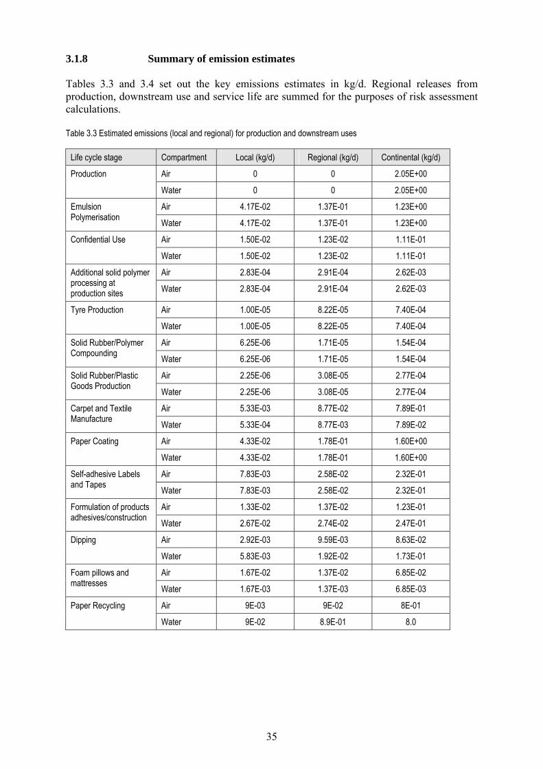
"Quantitative" Risk Assessment by comparison of exposure with effects The risks from the normal use of tert-dodecanethiol (TDM) to water, sediments, soil and predators have been assessed by the application of standard models to the information available. The property data set is far from complete for this purpose, and therefore there are areas of uncertainty, where further information could be valuable. This assessment therefore makes recommendations about the significance of the data gaps, and suggests where further research should be focussed. The research has involved searching publicly-available sources, and also extensive consultation with the producers and users of TDM and other thiols. The main use of these substances is as modifiers of the molecular weight distribution of such products as synthetic rubber and latex dispersions. TDM is by far the most important substance used for this purpose. As a highly-reactive reaction ingredient, it is largely consumed in the polymerisation reactions, although traces are left in the products. Therefore, some research into the uses of polymers has been made, to identify the potential for release of the TDM impurity present. The key life-cycle stages identified by industry research and potential emissions to the environment from these uses were estimated on the basis of site visits and the Emission Scenario Documents. Using the available information, PEC/PNEC values above 1, indicating an unacceptable risk for the environment, were identified for certain life-cycle stages, the most significant of these being emulsion polymerisation, paper coating, formulation of inks and adhesives and paper recycling. The main use, emulsion polymerisation, is the highest priority to study further, while uncertainties regarding the levels of residual TDM in polymers and dispersions should be clarified, to ascertain if further research into emissions from downstream industries is required. Some information provided by industry has been treated as confidential and not included in this report, although the data have been used to inform the development of appropriate emission scenarios. These data are included in a confidential annex supporting the assessment, which is available via the Project Manager where appropriate. It has been found that, in all probability, the only other thiol of importance in the UK is n-dodecanethiol (NDM), although the use of other thiols does occur. Therefore an assessment of the current use of NDM is also made. Conclusions for NDM are essentially the same as for TDM, given the similarity in use-pattern and the use of read-across of the key data used to derive PNECs. The overall conclusions of the risk assessment are:

1. There are risks associated with certain life cycle stages, as indicated in the table overleaf.

RCR values > 1 were also identified for secondary poisoning, but these results are based on a limit value from a non-standard mammalian test which showed no effects.

viii

Life cycle stage Compartment Emulsion Polymerisation Freshwater sediment

Seawater Marine sediment

Confidential Use Freshwater sediment Seawater Marine sediment

Carpet and Textile Manufacture Marine sediment Paper Coating Freshwater sediment


Self-adhesive tapes and labels Seawater Marine sediment

Formulation of products for inks/adhesives/construction

Freshwater sediment Seawater Marine sediment

Dipping Seawater Marine sediment

Foam pillows and mattresses Marine sediment Paper Recycling Freshwater sediment


These risks are identified using the best information available. There are many data gaps, and where these occur estimates have been made, which inevitably increase the uncertainty in any risk identified and conclusion drawn. It is recognised that further information on both the intrinsic properties of the thiols and the use pattern and emissions may help reduce this level of uncertainty. This information should include:

2. Further information on use pattern and emissions from users of TDM in respect of uses identified as producing a risk, and in particular that associated with the main use, emulsion polymerisation. Such further information could include:

Emulsion polymerisation:

• Statistically analysed site-specific data on emissions, in compliance with the TGD* e.g. effluent monitoring.

• Site-specific dilution factors rather than the defaults currently used. Confidential use:

• Further information on site sizes, locations and emissions.

Downstream use of polymer dispersions:

* Section 2.2 of the TGD sets out criteria for assessing measured environmental concentration data. These principles can also be applied to effluent monitoring data. According to the TGD, the most important factors to be addressed are the analytical quality control and the representativeness of the sample. Information on the analytical method, validation, and details of the sampling regime in relation to the process, are therefore required.

ix

Once measured data on residues become available (see conclusion 3), a re-assessment will be required. If a risk is still indicated, further in-depth investigation of these life-cycle stages will be required, such as:

• More accurate emission estimates and possibly effluent monitoring. • Locations of sites will need to be identified with respect to marine risk

assessment. Paper recycling:

• Further investigation of the potential for degradation of TDM in the paper recycling process.

• If degradation does not occur, further investigation as for other downstream stages.

3. The amount of residual TDM present in rubber and polymer dispersions made by all

major producers should be determined. 4. The significance of analytical determinations of TDM in sediment, performed by the

Environment Agency, needs further investigation. 5. The need for further laboratory testing should be reviewed after these other points

have been addressed. The main consideration would be the need for toxicity tests for sediment-dwelling organisms.

It is also noted that n-dodecanethiol (NDM) is believed to have a similar life cycle and properties, and any discussions on TDM should include it also. A risk assessment for NDM is given in the confidential annex. Follow up action being undertaken by Industry The Environment Agency met with representatives of TDM producers and users in November 2004. The industry representatives agreed that further work is required to refine the risk assessment. They have agreed to develop an analytical method to measure residual TDM concentrations in polymer dispersions and, if the method is applicable, to determine the residual concentrations of TDM in polymer dispersions and solid polymers over the next 12 months. Industry has also agreed to conduct a test to determine the potential for oxidation of TDM in aqueous media and results should be available within 6 months. If TDM does not oxidise, further work on its persistence will be conducted. Follow-up action being taken by the Environment Agency It is recognised that this assessment could be influenced by further information and that the current conclusions are uncertain. This report has therefore identified these uncertainties. Once the additional information generated by industry becomes available, the Agency will consider this and all other new relevant information and its impact on the risk assessment conclusions. We may therefore update the report at some future date.

x

Based on the information currently available, TDM poses a potential risk to the environment in the UK. It is a candidate PBT substance and risks have been identified to sediment using the quantitative risk assessment approach in the EU Technical Guidance Document.

xi

Acknowledgements We would like to thank all the members of the Mercaptans/Thiols Council, IISRP, and Cefic sector groups EPDLA and ABS/SAN who participated in the industry consultation. Site visits to Zeon Chemicals Europe Ltd (polymerisation) and Heckmondwike FB (fibre-bonded carpets) are also acknowledged with gratitude. Finally, we thank John Fardon of the Environment Agency’s laboratory in Leeds for assistance with the sediment monitoring data.

xii

CONTENTS

1 GENERAL SUBSTANCE INFORMATION ................................................................. 1 1.1 IDENTIFICATION OF THE SUBSTANCE .................................................. 1

1.2 PURITY/IMPURITIES, ADDITIVES ............................................................ 3 1.2.1 Purity/impurities ................................................................................................................................3 1.2.2 Additives 3

1.3 PHYSICO-CHEMICAL PROPERTIES......................................................... 3 1.3.1 Physical state (at ntp).........................................................................................................................3 1.3.2 Melting point .....................................................................................................................................4 1.3.3 Boiling point ......................................................................................................................................4 1.3.4 Relative density .................................................................................................................................4 1.3.5 Vapour pressure.................................................................................................................................4 1.3.6 Water solubility .................................................................................................................................4 1.3.7 n-Octanol-water partition coefficient.................................................................................................4 1.3.8 Hazardous physico-chemical properties ............................................................................................6 1.3.9 Other relevant physico-chemical properties ......................................................................................7 1.3.10 Summary of key physico-chemical properties...................................................................................7

1.4 KEY PROPERTIES OF NDM......................................................................... 8

2 GENERAL INFORMATION ON EXPOSURE............................................................. 9 2.1 PRODUCTION.................................................................................................. 9

2.2 USES ................................................................................................................... 9 2.2.1 General information on uses ..............................................................................................................9 2.2.2 Emulsion Polymerisation.................................................................................................................11 2.2.3 Synthetic Rubber .............................................................................................................................17 2.2.4 Tyre Manufacture ............................................................................................................................18 2.2.5 Other solid polymer products ..........................................................................................................19 2.2.6 Polymer Dispersions........................................................................................................................19

2.3 TRENDS........................................................................................................... 23

2.4 LEGISLATIVE CONTROLS ........................................................................ 23

3 ENVIRONMENTAL EXPOSURE................................................................................ 24 3.1 ENVIRONMENTAL RELEASES................................................................. 24 3.1.1 General introduction ........................................................................................................................24 3.1.2 Releases from production ................................................................................................................25 3.1.3 Releases from emulsion polymerisation ..........................................................................................25 3.1.4 Releases from a confidential use .....................................................................................................25 3.1.5 Releases from downstream processing ............................................................................................25 3.1.6 In-service loss ..................................................................................................................................30 3.1.7 Releases from disposal ....................................................................................................................31 3.1.8 Summary of emission estimates ......................................................................................................35

3.2 ENVIRONMENTAL FATE AND DISTRIBUTION................................... 37 3.2.1 Atmospheric degradation.................................................................................................................37 3.2.2 Aquatic degradation.........................................................................................................................37 3.2.3 Degradation in soil...........................................................................................................................38 3.2.4 Evaluation of environmental degradation data ................................................................................38 3.2.5 Environmental partitioning..............................................................................................................38 3.2.6 Adsorption .......................................................................................................................................39 3.2.7 Volatilisation ...................................................................................................................................39 3.2.8 Precipitation.....................................................................................................................................40 3.2.9 Bioaccumulation and metabolism....................................................................................................40 3.2.10 Environmental properties of predicted oxidation products..............................................................40 3.2.11 Summary of environmental fate and distribution ............................................................................42

xiii

3.3 ENVIRONMENTAL CONCENTRATIONS................................................ 43 3.3.1 Aquatic compartment (surface water, sediment and wastewater treatment plant) ...........................43 3.3.2 Terrestrial compartment...................................................................................................................46 3.3.3 Atmospheric compartment...............................................................................................................46 3.3.4 Food chain exposure ........................................................................................................................48

3.4 MARINE EXPOSURE ASSESSMENT ........................................................ 49

4 EFFECTS ASSESSMENT: HAZARD IDENTIFICATION AND DOSE (CONCENTRATION) - RESPONSE (EFFECT ASSESSMENT)............................. 50

4.1 AQUATIC COMPARTMENT (INCLUDING SEDIMENT) ..................... 50 4.1.1 Toxicity to fish.................................................................................................................................51 4.1.2 Toxicity to aquatic invertebrates......................................................................................................51 4.1.3 Toxicity to algae ..............................................................................................................................52 4.1.4 Toxicity to microorganisms.............................................................................................................52 4.1.5 Toxicity to amphibians ....................................................................................................................53 4.1.6 Toxicity to sediment-dwelling organisms........................................................................................53 4.1.7 Predicted No Effect Concentrations (PNECs) for the aquatic compartment ...................................57

4.2 TERRESTRIAL COMPARTMENT............................................................. 58 4.2.1 Terrestrial toxicity data....................................................................................................................58 4.2.2 Calculation of PNEC for the soil compartment ...............................................................................58

4.3 ATMOSPHERIC COMPARTMENT ........................................................... 59

4.4 NON-COMPARTMENT SPECIFIC EFFECTS RELEVANT TO THE FOOD CHAIN (SECONDARY POISONING)............................................. 59

4.4.1 Mammalian toxicity data .................................................................................................................59 4.4.2 Derivation of PNECoral.....................................................................................................................60

4.5 MARINE EFFECTS ASSESSMENT ............................................................ 61 4.5.1 PBT assessment ...............................................................................................................................61 4.5.2 Marine toxicity data.........................................................................................................................62 4.5.3 Calculation of Predicted No Effect Concentration (PNEC).............................................................62

4.6 CLASSIFICATION FOR ENVIRONMENTAL HAZARD........................ 62

5 RISK CHARACTERISATION ..................................................................................... 63 5.1 AQUATIC COMPARTMENT....................................................................... 63 5.1.1 Surface water and sediment .............................................................................................................63 5.1.2 The concept of critical release rate ..................................................................................................65 5.1.3 Wastewater treatment plant (WWTP) micro-organisms..................................................................66

5.2 TERRESTRIAL COMPARTMENT............................................................. 66 5.2.1 Risk characterisation ratios..............................................................................................................66 5.2.2 Conclusion for soil...........................................................................................................................66

5.3 ATMOSPHERIC COMPARTMENT ........................................................... 66 5.3.1 Conclusion for the atmosphere ........................................................................................................66

5.4 NON-COMPARTMENT SPECIFIC EFFECTS RELEVANT TO THE FOOD CHAIN (SECONDARY POISONING)............................................. 67

5.4.1 Risk characterisation ratios..............................................................................................................67 5.4.2 Conclusion for predators..................................................................................................................67

5.5 MARINE ASSESSMENT ............................................................................... 69 5.5.1 Risk characterisation ratios..............................................................................................................69 5.5.2 Conclusion for the marine environment ..........................................................................................70

5.6 SUMMARY OF CONCLUSIONS ................................................................. 70 5.6.1 PBT Assessment ..............................................................................................................................70 5.6.2 “Quantitative” Risk Assessment......................................................................................................70

6 REFERENCES................................................................................................................ 73

xiv

7 ABBREVIATIONS ......................................................................................................... 76 APPENDIX 1 PROGRAM OUTPUTS FROM EPIWIN VERSION 3.11......................... 78

APPENDIX 2 REVIEW OF A KEY REFERENCE BOOK............................................... 95

APPENDIX 3 EUSES 2.0 ...................................................................................................... 105

APPENDIX 4 DISCUSSION OF DEGRADATION OF TDM.......................................... 106

APPENDIX 5 ROBUST STUDY SUMMARIES AND DISCUSSION ............................ 108

1

1 GENERAL SUBSTANCE INFORMATION Information has been obtained from the most recent reliable sources. In particular, the industry sector group Mercaptans/Thiols Council has compiled a data set in IUCLID format (MTC, 2003). This is not yet publicly available. 1.1 IDENTIFICATION OF THE SUBSTANCE There is some ambiguity in published literature about the composition of the substance; this is discussed below. The primary information is based on that available from the IUCLID 2000 CD-ROM. CAS Number: 25103-58-6 EINECS Number: 246-619-1 IUPAC Name: tert-dodecanethiol EINECS name: tert-dodecanethiol Molecular formula: C12H26S Synonyms: Tert-dodecylmercaptan (IUCLID 2000) 2,2,4,6,6-pentamethyl-4-heptanethiol (IUCLID 2000) Sulfole® 120 (IUCLID 2000) TDM (IUCLID 2000) t-DDM (CAS, 2004) tert-laurylmercaptan (CAS, 2004) Note: the synonym tert-dodecylmercaptan (the origin of the abbreviation TDM) is common nomenclature, which is still in use in most areas of the industry. Although the common abbreviation TDM is used throughout this report, the standard ‘thiol’ nomenclature is now preferred and is used herein. A similar situation exists for the related substance n-dodecylmercaptan (NDM), now known as n-dodecanethiol, and other substances. Isomers The majority of TDM is produced using propylene tetramer as the feedstock (Pers. Comm., January 2005).

2

A typical propylene tetramer feedstock contains the following (Source: Chevron Oronite 2004): Component % by weight ≤ C10 3.5 C11 13.7 C12 50.5 C13 18.9 C14 10.3 ≥ C15 3.1 Other producers of propylene tetramer will have different specifications, and typical ranges for distribution of components are as follows (Pers. Comm., August 2004): Component % by weight ≤ C10 <10 C11 15-20 C12 50-80 C13 2-20 ≥C14 <15 Another route to the alkyl chain in TDM is the trimerisation of isobutylene. Both routes result in a highly branched alkyl chain, consisting of a mixture of isomers. CAS number 25103-58-6 is listed in the CAS registry and IUCLID 2000 as tert-dodecanethiol, but the structure is not specified. The IUCLID 2000 entry also specifies 2,2,4,6,6-pentamethyl-4-heptanethiol, CAS No 93002-38-1 (Phillips Petroleum Company). The ChemFinder entry (www.chemfinder.cambridgesoft.com) for CAS No 25103-58-6 is listed as 2,3,3,4,4,5-hexamethyl-2-hexanethiol, but this name is not recognised by the CAS registry. Within the EPIWIN v3.11 structure database (SRC, 2000), the SMILES Code for CAS No 25103-58-6 is listed for 4-butyl-4-octanethiol. However, this is not considered to be truly indicative of the degree of branching that is expected. 2,2,4,6,6-pentamethyl-4-heptanethiol is considered to be the best-supported representative structure for TDM. However, in respect of the data available, their interpretation and use within models, the differences in properties that might exist between various hypothetical isomers is not considered to be important.

3

Structural formula: CH3C(CH3)(CH3)CH2C(CH3)(SH)CH2C(CH3)(CH3)CH3 Representative structure:

CH3CH3

CH3

CH3

SH

CH3

CH3

CH3

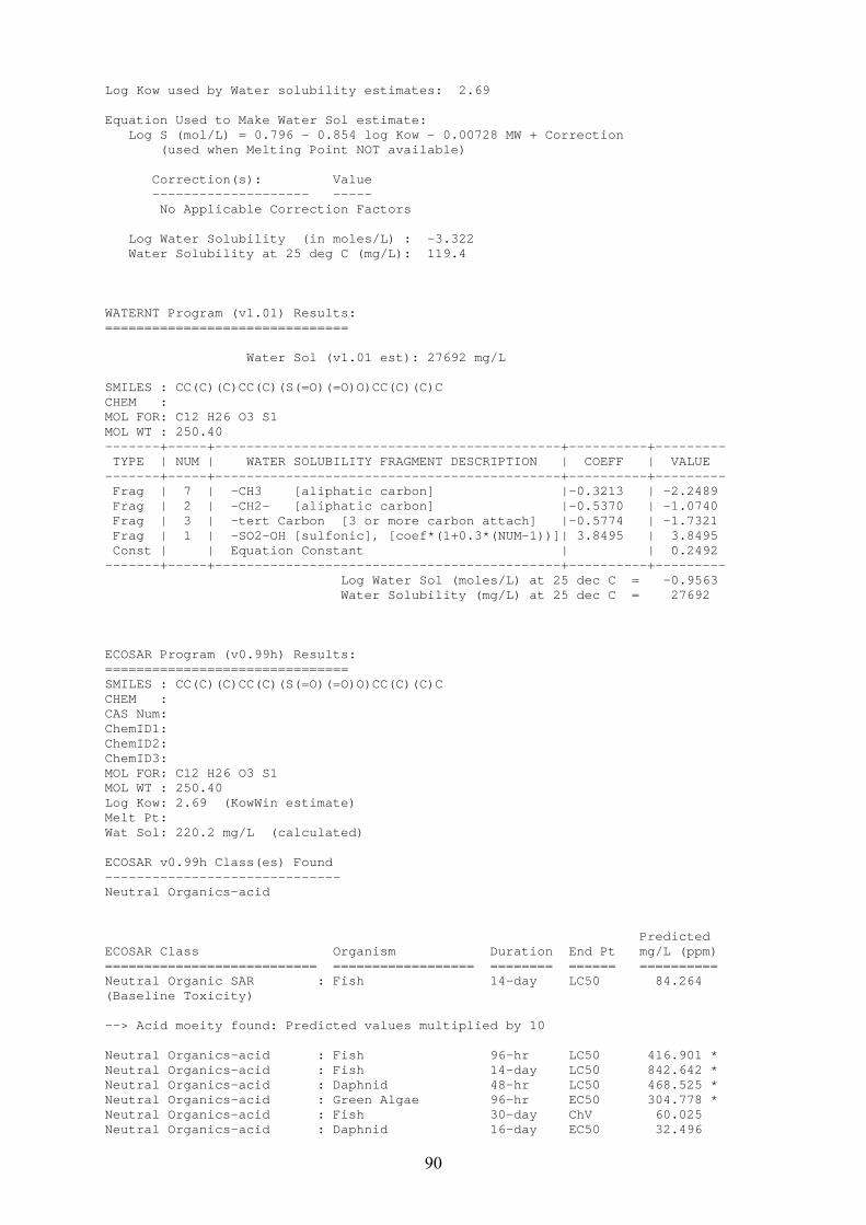
SMILES Code: CC(C)(C)CC(C)(S)CC(C)(C)C Molecular weight: 202.4 g/mole 1.2 PURITY/IMPURITIES, ADDITIVES 1.2.1 Purity/impurities Commercial batches of TDM are typically > 95% pure, although this may refer to a mixture of isomers and carbon chain length fractions. Impurities are typically olefins and light mercaptans and sulfides. Further discussion of composition is included in the confidential annex. 1.2.2 Additives There are no reported additives used with TDM (MTC 2003). 1.3 PHYSICO-CHEMICAL PROPERTIES The following section provides a summary of the chemical and physical properties of TDM. Summary test reports were provided for key vapour pressure and water solubility data, as described below. The test reports were reviewed and are summarised in the confidential annex. Original reports of other studies cited in IUCLID have not been reviewed since these were not provided by the study sponsors. Alkylthiols with different chain lengths present in the commercial TDM product will have different physico-chemical properties. The differences in properties are expected to be small and will therefore not affect the present conclusion of the PBT assessment, and it is unlikely that they will have a significant impact on the outcome of the quantitative risk assessment. 1.3.1 Physical state (at ntp) Commercially produced tert-dodecanethiol is liquid at 20oC and 101.3 kPa (IUCLID 2000).

4

1.3.2 Melting point The melting point is reported in the industry IUCLID (MTC, 2003) as ca. –46°C from a GLP study conducted according to test guideline Method A1, 92/69/EEC (Bayer internal study, 1988). Other results reported are –45°C (Phillips Petroleum Company) and <-30°C (Elf Atochem Safety Data Sheet, 1990). 1.3.3 Boiling point The boiling point range is reported in the industry IUCLID (MTC, 2003) as 227 – 248°C at 1013 hPa, cited as handbook data from The Dictionary of Substances and Their Effects (DOSE, 2nd electronic edition). Other results reported are 84 – 106°C at 6 hPa (Elf Atochem Safety Data Sheet, 1990), 220°C at 1013 hPa (Bayer AG data) and 225 – 230°C at 1000 hPa (Phillips Petroleum Company). The results are in line with expectations from the EPIWIN estimation of 215°C. The EPIWIN outputs are reported in Appendix 1. 1.3.4 Relative density The relative density is reported in the industry IUCLID (MTC, 2003) as 0.86 g/cm3 at 20°C (Bayer AG data). 1.3.5 Vapour pressure The vapour pressure is reported in the industry IUCLID (MTC, 2003) as 4 hPa at 20°C from a non-GLP study conducted according to test guideline Method A4, 92/69/EEC (Bayer internal study, 1989). The full test report was not available for review. Other results reported are 14 hPa at 50°C (Bayer AG data), and 0.8 hPa at 50°C (Elf Atochem Safety Data Sheet, 1990). The results are in line with expectations from the EPIWIN estimation of 0.171 mmHg, equivalent to 0.228 hPa. The EPIWIN outputs are reported in Appendix 1. The measured value of 4 hPa will be used for the purposes of the risk assessment. 1.3.6 Water solubility The solubility in water is reported in the industry IUCLID (MTC, 2003) as 0.25 mg/l at 20°C in a GLP study (Bayer AG data). A summary report was available for review. The test used a non-guideline protocol. The result is in line with expectations from the EPIWIN estimation of 0.43 mg/l using WSKOWWIN or 1.30 mg/l using the fragment method WATERNT. The EPIWIN outputs are reported in Appendix 1. The measured value of 0.25 mg/l will be used for the purposes of the risk assessment. 1.3.7 n-Octanol-water partition coefficient The log Kow of TDM was determined to be > 6.2 in a recent GLP study conducted according to test guideline Method A8, 92/69/EEC, HPLC method (MTC, 2004). This value will be used for the purposes of the risk assessment. The calculated log Kow value (KOWWIN v1.67, SRC, 2000) is reported as 6.07 (Industry IUCLID, MTC, 2003). A calculated log Kow value of 6.1 is also reported (CLOGP v3.54). A

5

log Kow value of 5.85 was obtained for 2,2,4,6,6-pentamethyl-4-heptanethiol using KOWWIN v1.67 (SRC, 2000), as shown in Appendix 1. Predicted values are consistent with the measured result.

6

1.3.8 Hazardous physico-chemical properties A flash point result of 82°C is reported in the industry IUCLID (MTC, 2003), using a closed cup method according to test guideline DIN 51758 (Bayer AG data). Other results reported are 95°C using a closed cup method according to test guideline ASTM D93 (Elf Atochem Safety Data Sheet, 1990) and 96°C, cited as handbook data from The Dictionary of Substances and Their Effects (DOSE, 2nd electronic edition). The self-ignition temperature is reported as 230°C (Phillips Petroleum Company).

7

1.3.9 Other relevant physico-chemical properties 1.3.9.1 Viscosity The viscosity is reported as 3.36 mPa.s (Elf Atochem Safety Data Sheet, 1990, Industry IUCLID, MTC, 2003). 1.3.9.2 Henry’s Law constant No experimentally determined Henry’s law constant information is available, but this may be calculated from the vapour pressure, molecular weight and water solubility of the substance. Using values measured at 20°C (vapour pressure 400 Pa and water solubility 0.25 mg/l) gives a Henry’s Law Constant of 3.24E+05 Pa.m3/mol. The result is a little higher than expectations from the EPIWIN estimation of 5900 Pa.m3/mol, using the 'bond' method. The EPIWIN outputs are reported in Appendix 1. It is relevant to note that this value is sufficiently high to suggest that performance of any study involving aqueous solutions would necessitate the use of methods to limit volatile losses. EUSES 2.0 extrapolates measured vapour pressure and water solubility results to 25°C, giving values of 564 Pa and 0.268 mg/l respectively. Using these values gives a Henry’s Law Constant of 4.27E+05 Pa.m3/mol. This value will be used for the risk assessment. 1.3.10 Summary of key physico-chemical properties A summary of the key physico-chemical data used for the risk assessment of TDM is given in Table 1.1. Table 1.1 Physico-chemical properties of TDM

Property Value and comment

Physical state at ntp Liquid

Molecular weight 202.4 g/mol

Vapour Pressure 400 Pa at 20°C (Method A4, 92/69/EEC, non-GLP)

Water solubility 0.25 mg/l at 20°C (Simplified flask method, GLP)

n-Octanol-water partition coefficient (Kow) >6.2 (Method A8, 92/69/EEC, GLP)

Henry’s Law constant 4.27E+05 Pa.m3/mol (Calculated)

8

1.4 KEY PROPERTIES OF NDM A summary of the key property data for NDM is given in Table 1.2. Table 1.2 Physico-chemical properties of NDM

Property Value and comment

Physical state at ntp Liquid

Molecular weight 202.4 g/mol

Vapour Pressure 399 Pa at 25°C (Industry IUCLID, MTC, 2003)

Water solubility < 0.14 mg/l (HSDB)

0.225 mg/l (WSKOWWIN, SRC, 2000)

n-Octanol-water partition coefficient (Kow) 6.18 (KOWWIN, SRC, 2000)

Henry’s Law constant 3.59E+05 Pa.m3/mol (Calculated)

9

2 GENERAL INFORMATION ON EXPOSURE Regarding production, some information has been provided by the companies which import into the UK. Tonnage data have been set as ranges in order to avoid revealing commercially-sensitive information. Regarding 'downstream uses', information from consultees corroborates that from public sources, but again information from the consultees cannot be reported in detail in the present report due to commercial sensitivity. All tonnages reported are annual figures and, unless stated otherwise, refer to the EU prior to accession of ten new Member States in May 2004. No information on total consumption of polymer dispersions is available from industry; therefore data gathered from research will be used as far as possible to estimate the scale of downstream applications. Further description of the downstream industry is included in Appendix 2. In some cases, it is not possible to attribute the source of information, for reasons of confidentiality. 2.1 PRODUCTION TDM is produced at three sites in the EU, located in France, Germany and Belgium. There is no UK production. Details of the production sites and tonnages are provided in Chapter 2 of the confidential annex, but an indicative tonnage range of TDM in Europe is 10 to 25 ktonne. 2.2 USES 2.2.1 General information on uses Information about the application industries has been drawn from several published sources and to avoid over-referencing these include:

The emission scenario for rubber additives in the Risk Assessment Technical Guidance Document (EC, 2003) The IISRP web site (www.iisrp.com) Polymer Dispersions and their Industry Applications (Urban and Takamura, 2002) Polymers:Chemistry and Physics of Modern Materials (Cowie, 1991)

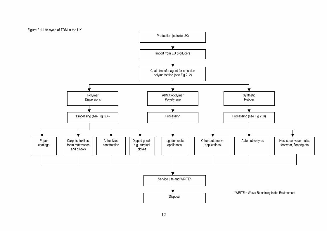
The life-cycle of TDM in UK industry is illustrated in Figure 2.1. Its main use is as a chain transfer agent in the production of emulsion polymers, particularly styrene butadiene rubber (SBR or E-SBR) and acrylonitrile butadiene, or nitrile, rubber (NBR). Thus releases to the environment could occur during this main use. Whilst TDM should be considered primarily as a reactive intermediate, it is possible that it could be released from rubber during all of these life cycle stages, either as a trace impurity in the rubber, or (less likely) by degradation of the rubber. These possibilities are discussed in more detail below. Solid SBR and NBR are widely used throughout the world for numerous and diverse applications. The worldwide production capacity for SBR exceeds 2 million tonnes per annum (IISRP, 2004), while consumption of NBR is expected to reach 368,000 tonnes per annum by 2005 (IISRP, 2004). The

10

predominant use of solid SBR is in automotive tyre treads. Other uses include automotive applications such as mats and beading; footwear; food contact materials including conveyor belts and container seals; hoses; gaskets; wires and cables and other rubber goods. SBR is resistant to many polar solvents including dilute acids and bases, but swells on contact with non-polar solvents. NBR is more suitable for use in applications such as fuel and oil handling hoses, seals etc., as well many other industrial and general rubber products. Production capacities for solid rubbers using TDM in the UK are 70, 000 and 15, 000 tonnes per annum for SBR and NBR respectively. (IISRP Worldwide Rubber Statistics). This industry is broadly represented by the International Institute of Synthetic Rubber Producers (IISRP, see www.iisrp.com), and the EU members of this organisation who use TDM have participated in the research and provided production and sales data. A total of between 50 and 75 kt solid E-SBR and NBR are consumed per annum in the UK and Ireland (IISRP, 2004). Approximately two-thirds of this is believed to be used at large sites, mainly for tyre production, while the remaining third is used at smaller sites for production of other types of rubber goods. The other major use, and the predominant industry relevant to TDM use in the UK, is in the production of emulsion polymer dispersions and latices*, which also uses an emulsion polymerisation technique. In this case, products are supplied and further processed in the form of aqueous dispersions, which typically have a solids content of 40 – 60% (Urban and Distler, 2002). These industries are represented largely by the European Polymer Latex and Dispersion Association (EPDLA, see www.cefic.be) and most of the UK members and some members from other European countries have participated in the research and provided production and sales data. A detailed breakdown of these data is given in the confidential annex. Typical applications of SBR and NBR polymer dispersions produced using TDM are carpet backing and underlay, textiles, paper coatings, adhesives, dipped rubber goods and products for the construction industry. Data on the net consumption of these products in the UK are not currently available from industry. High solids latex (HSL) is produced from the base latex from the polymerisation process, which is circulated through wipe film evaporators until the desired solids content is achieved. HSL can be used in the manufacture of foam pillows and mattresses (Pers. Comm, August 2004). A less important use of TDM is in emulsion polymerisation of acrylonitrile-butadiene styrene (ABS) plastics used for applications such as automotive parts, domestic appliances (vacuum cleaners, fridges, hairdryers) and toys. A small proportion is also used as a chain transfer agent in emulsion polystyrene production. Loading rates of TDM may be much lower than for these applications than for SBR and NBR polymers. Use of TDM for applications other than as a chain transfer agent have also been indicated by industry and are described in the confidential annex. * The term ‘latexes’ can also be used as the plural of latex. Note that the terms “polymer dispersion”, “emulsion polymer” and “latex” are used synonymously by industry to describe aqueous dispersions of synthetic polymers. The term “latex” is also used to describe natural rubber dispersions. For the purposes of this report, the term “polymer dispersion” will be used.

11

2.2.2 Emulsion Polymerisation A breakdown of the tonnage of TDM used in the UK is given in the confidential annex. The main use of TDM is as a chain transfer agent for emulsion polymerisation. Emulsion polymerisation is a process whereby monomers are dispersed in an aqueous system using an emulsifying agent, and a water-soluble initiator is employed. The emulsion polymerisation process has several advantages over bulk polymerisation (where the reaction mixture contains only monomer and initiator). Benefits include the fact that emulsion polymerisation gives high solids contents with low reaction viscosity and is a cost-effective process. Problems encountered in bulk polymerisation, for example the build-up of hotspots due to the exothermic nature of the reaction, or gel formation, are much less important in emulsion processes. Polymerisation reactions are carried out either as batch or continuous processes. In batch production, all the ingredients are loaded to the reactor and polymerisation is shortstopped (terminated using an agent which reacts rapidly with free radicals), after it reaches the desired conversion. Other commercial productions are run continuously by feeding reactants and polymerising through a chain of reactors before shortstopping at the desired monomer conversion. Figure 2.2 shows a simplified outline of the emulsion polymerisation process. In the emulsion system, polymer chain length can be controlled by temperature without affecting the reaction rate. Temperature also influences the degree of branching in the polymer and the stereochemistry of butadiene units in the chain. E-SBR and NBR are produced using both “hot” and “cold” processes resulting in polymers with differing properties. The “cold” polymerisation is typically carried out at 5 to 15°C and yields more linear structures, which are easier to process and have superior surfaces. “Hot” polymerisation is carried out at temperatures of 30 to 40°C and yields highly branched structures, giving them superior green strength* and making them suitable for use in applications where shape retention or adhesive properties are desired.

* Ability of material to undergo handling without distortion.

12

Figure 2.1 Life-cycle of TDM in the UK

* WRITE = Waste Remaining in the Environment

Production (outside UK)

Import from EU producers

Chain transfer agent for emulsion polymerisation (see Fig 2. 2)

Paper coatings

Carpets, textiles, foam mattresses

and pillows

Adhesives, construction

Dipped goods e.g. surgical

gloves

e.g. domestic appliances

Hoses, conveyor belts, footwear, flooring etc

Automotive tyresOther automotive applications

Processing (see Fig 2. 3)Processing (see Fig 2.4)

ABS Copolymer Polystyrene

Processing

Service Life and WRITE*

Disposal

Polymer Dispersions

Synthetic Rubber

13

Figure 2.2 Emulsion polymerisation process

Reactor chain or batch reactor

Monomers Emulsifier Initiator Water

Latex dispersion

Shortstop

Unreacted monomer

Blending tanks

Antioxidant Other additives

Finishing (excess water removed)

Coagulating agent

Coagulated crumb rubber

Packaging (e.g. bales)

TDM

Synthetic rubber processing (see Fig. 2.3)

Packaging (e.g. drums, tanks)

Polymer dispersion processing (see Fig. 2.4)

14

Figure 2.3 Synthetic rubber processing

Synthetic or

Natural Rubber

Mastication physical

thermo-physical chemical

Shaping moulding extrusion

calendering

Vulcanisation sulphur

peroxides phenolic resins

Finishing

Final rubber goods

15

Figure 2.4 Example of polymer dispersion processing

Aqueous Latex Emulsion

Drying

Coagulation (dipping, shaping)

Compounding

Stabilisation

Surfactants, antioxidants. pH control, anti-microbial and anti-foaming agents

Curing

e.g. wetting agent, thickener, preservative, vulcanisation agents,

fillers

Coagulating agents, heat sensitisers

Coating

16

Table 2.1 shows the raw materials typically required in the polymerisation of E-SBR, which include monomers (styrene and butadiene), water, emulsifier, initiator system, modifier, shortstop and a stabiliser system (IISRP, 2004). Table 2.1: Typical reaction mixture for SBR emulsion polymerisation

Component Composition of reaction mixture (Parts by Weight)

Cold Hot

Styrene 25 25

Butadiene 75 75

Water 180 180

Emulsifier 5 5

TDM 0.2 0.8

Cumene hydroperoxide 0.17 -

Ferrous sulfate FeSO4 0.017 -

EDTA 0.06 -

Sodium phosphate Na4P2O7.10H2O 1.5

Potassium persulfate 0.3

Sodium formaldehyde sulfoxide 0.1

Stabiliser varies Chain termination in free radical polymerisation usually occurs when two active radical centres attached to polymer chains combine. However, termination can also take place if activity is transferred to another species, such as a monomer, a polymer chain (leading to branching), or a modifier. Thus, the addition of a chain transfer agent allows the molecular weight of the polymer to be controlled while initiating a new chain. Alkylthiols are suitable for this purpose since the S – H bond is weaker than C – H and is therefore susceptible to attack by the growing polymer radical: CH2CHX• + RSH CH2CH2X + RS• RS• + CH2=CHX RSCH2CHX• Concentration of alkylthiol in the reaction mixture and the relative rate constants of chain transfer versus polymerisation determine the final chain length. During polymerisation, parameters such as temperature, flow rate and agitation are controlled to achieve the right conversion. Polymerisation is normally allowed to proceed to about 60% conversion in cold polymerisation and 70% in hot polymerisation before it is terminated with a shortstop agent. Historically, common shortstopping agents were sodium dimethyldithiocarbamate and diethyl hydroxylamine, although these have been replaced with isopropyl hydroxylamine due to the potential formation of nitrosamines in the latex (Pers. Comm., August 2004). In the production of polymer dispersions, polymerisation is often conducted to a very high degree of monomer conversion, for example 98% or higher, so no shortstop agent is required (Pers. Comm., April 2004). The loading rate of TDM into the polymerisation mixture is variable depending on the application and the required product characteristics, but is typically in the range 0.01 – 2%.

17

After polymerisation, it could reasonably be expected that trace levels of unreacted TDM may remain in the polymer, although there is disagreement between users of TDM. Measurement of residual TDM is not routinely carried out. In the absence of analytical data, industry has provided us with estimates of the concentrations remaining in solid polymer products (Pers. Comm., 2004a) and in polymer dispersions (Pers. Comm., 2004b). Further details are provided in the confidential annex. TDM is known to have a strong, unpleasant odour, with a reported odour threshold in air of 0.1 – 0.6 ppm (Chevron Phillips MSDS). However, it is not known what concentration in polymer or dispersion would be considered unacceptable by downstream customers. As discussed further in section 3.1.5.1, due to the adsorption properties of TDM, it is expected that only around 1% of the residual TDM in dispersions would be available for volatilisation to air. Assuming the worst case that all of this is volatilised, and taking dilution in air into account, a worst-case value of 100 ppm in polymer/dispersion would be around the limit of detection by humans. 2.2.3 Synthetic Rubber 2.2.3.1 Production Once polymerisation is properly shortstopped, unreacted monomers are stripped off and recycled. The emulsion can then be stabilised with an appropriate antioxidant and transferred to blend tanks where other additives can be incorporated according to requirements (e.g. carbon black filler for tyres; mineral oil in production of oil-extended substrates). The emulsion is transferred to finishing lines to be coagulated using a system appropriate to the end-use of the product (e.g. sulfuric acid/sodium chloride; glue/sulfuric acid; amines). The coagulated crumb rubber is then washed, dewatered, dried, baled and packaged. Addition of antioxidants is not relevant for all applications (Pers. Comm., 2004). 2.2.3.2 Processing Further processing of solid rubber is not carried out by the major rubber producers in the UK. Generally, the baled crumb rubber is sold on to numerous rubber compounders and manufacturers of finished goods. According to the Emission Scenario Document for Rubber Additives (UBA, 2003), the key stages of rubber processing are mastication; shaping; vulcanisation and finishing. Compounding with additives such as vulcanising agents, processing aids, anti-degradants, fillers, colorants and others can take place during production (before coagulation), or during mastication. 2.2.3.2.1 Mastication Mastication is the physical working of solid rubber to reduce molecular weight and hence lower viscosity and improve workability. Mastication may be carried out at high or low temperature using internal mixers or rolling mills. Alternatively, plasticisers, chemical peptisers or lubricants can be added to the mixture. Water may be used as a coolant, in direct contact with the rubber mixture, although no specific instances of this have been identified. This step is not applicable to SBR (Pers. Comm, August 2004).

18

2.2.3.2.2 Shaping Shaping of rubber goods is carried out using the normal techniques of the polymers industry, including extrusion, calendering and moulding. For further explanation of these terms, refer to the Emission Scenario Document for plastics additives (EA 2003a). 2.2.3.2.3 Vulcanisation Vulcanisation is used to introduce cross-linking between individual polymer strands and thus improve the elastic properties of the rubber. Without vulcanisation, the rubber is brittle and can suffer from surface tackiness. Vulcanising agents such as elemental sulfur, metal dithiocarbamates or organic peroxides are added to the rubber mixture either prior to coagulation or during mastication. After shaping, goods are cured at the required temperature using a variety of techniques including in-mould curing, hot air curing after ultra-high frequency pre-heating or curing in a liquid bath. 2.2.3.2.4 Finishing Finishing processes could include, for example, trimming of excess rubber. 2.2.4 Tyre Manufacture As discussed in section 2.2.1, up to 50,000 tonnes of solid rubber may be used for this application in the UK. An Environment Agency report (EA, undated, 2) states that over 35 million tyres are manufactured in the UK each year, of which approximately 30 million are for road vehicles (also 28 million sold in UK; 27 million imported; 21 million exported). The tyre manufacturing process is complex and requires the mixing of various grades of natural and synthetic rubbers to achieve the desired properties of the tyre such as traction and abrasion resistance. Various types of SBR (e.g. hot and cold polymers, oil extended or styrene masterbatch) are used in the different components of the tyres. Blending (compounding) of the rubber mixture with carbon black, sulfur and other additives is carried out using internal mixers. The majority of rubber compounds are used to form tyre treads and sidewalls using extrusion techniques to produce a continuous sheet which is then cooled and cut to the required size. Calendering is used to coat woven textile or steel sheets with rubber to form plies in a continuous sheet which are then cut to size, and the bead core is produced by coating a steel wire with rubber and winding on to a coil to form a bead ring of the required size. Beginning with the woven plies, the bead rings, sidewalls and tread rubber are assembled on a building drum to achieve a “green tyre”, which is then placed in a mould in a curing press at the appropriate temperature and pressure for 10 to 15 minutes to obtain the final size, shape and tread pattern, before being ejected from the mould. Thirteen tyre manufacturing sites have been identified in the UK from the website of the British Rubber Manufacturers’ Association (BRMA, www.brma.co.uk), and other Internet research.

19

2.2.5 Other solid polymer products As discussed in section 2.2.1, up to 25,000 tonnes of solid rubber may be used for this application in the UK. Solid NBR and a small proportion of solid SBR are used in the manufacture of a wide variety of rubber products, including conveyor belts, seals; hoses; dairy components, gaskets; wires and cables and numerous specialised applications. Following compounding of the rubber mixture with other additives, the typical techniques used by the industry, are injection and compression moulding, extrusion, calendering etc. Although the end-uses of other emulsion polymers such as ABS and polystyrene are different to synthetic rubber, the life-cycle stages of compounding and shaping described for rubber are also applicable to these polymers. 2.2.6 Polymer Dispersions 2.2.6.1 Production The initial stages of polymer dispersion production are similar to synthetic rubber. Emulsion polymerisation takes place as described previously, usually using “hot” conditions, and a higher monomer conversion rate. However, instead of coagulation taking place at the production site, the polymer dispersion is stabilised by the addition of surfactants to prevent coagulation, antioxidants, antimicrobial agents, antifoaming agents and pH buffers. Other additives can also be blended at this stage according to requirements. The polymer dispersions are then packaged in drums or tankers for onward supply. 2.2.6.2 Compounding Compounding of the polymer dispersion with other additives takes place under aqueous conditions. Water immiscible additives are prepared as aqueous dispersions or emulsions, while water soluble substances can be added directly. Typically, additives such as vulcanising agents, wetting agents, fillers, thickeners and preservatives are used at this stage. For certain applications, special ingredients such as heat-sensitising compounds may be added. (www.rubber-compounding.com). 2.2.6.3 Processing Polymer dispersions are used mainly in applications such as carpet backing, paper coatings and adhesives, as well as the manufacture of dipped (e.g. gloves), cast (e.g. rubber toys) or extruded products (e.g. elastic threads, inner tubes), as well as coating, impregnation and foam production (www.rubber-compounding.com). The main downstream industries using emulsion polymers produced with TDM are briefly described in the following sections. Further details of applications relevant to the downstream industry in the UK are given in Appendix 2. No information on total consumption of polymer dispersions are available from industry, therefore data gathered from research will be used as far as possible to estimate the scale of downstream applications. Full justification of the tonnages used for calculations is given in Chapter 2 of the confidential annex.

20

2.2.6.3.1 Carpet Backing and Underlay Up to around 130,000 tonnes of polymer dispersion may be used per year in the UK for this application. Further information on tonnages and site sizes is given in Chapter 2 of the confidential annex. One of the major uses of SBR polymer dispersions in the UK is production of SBR foam backed carpets and carpet underlay. SBR latices can be used either as a backing coat, as in tufted carpets, or as a homogeneous binder in fibre-bonded carpets. Tufted carpets are generally used in residential applications, while fibre-bonded carpets are used for commercial or institutional applications such as schools or offices. Tufted carpet consists of a carrier layer (strips of fabric); pile yarn (inserted into the carrier material); a pre-coating layer (carboxylated SBR used to anchor the pile onto the carrier layer) and a coating layer (applied to the bottom side of the carpet). The coating layer is generally SBR foam, polyurethane foam or textile backing and its functions are to strengthen the attachment of the pile, improve dimensional stability and provide properties such as anti-slip, heat insulation or flame retardancy. Textile backed carpets are often used in combination with a separate felt or latex underlay to increase durability, heat insulation and comfort (BREF, 2003). Figure 2.5 illustrates the structure of a typical tufted carpet. Figure 2.5 Tufted carpet Primary backing = Polypropylene, polyester, jute Pre-coat = XSB (carboxylated styrene-butadiene) latex Adhesive = XSB latex Secondary backing = foam SBR, needlefelt, textile Tuft or pile (cut or loop) = Polypropylene, polyamide, polyester, wool, acrylic The polymer dispersions are formulated with a number of other ingredients including fillers, thickeners, flame retardants, colourants and pigments, stabilisers, foaming agents (surfactants) and vulcanisation agents and accelerants. The formulation is typically foamed with air and then applied to the carpet using a doctor-blade. The foam is then stabilised using

21

either surfactants or ammonium acetate or silicium fluoride gelling systems, and solidified and dried in a vulcanisation oven (BREF, 2003). In the production of fibre-bonded carpet, felt is produced from short strands of combed and carded man-made fibres, which is then compressed using a needlepunch technique. The compressed felt is fully impregnated with latex dispersion to bind the fibres. Pre-formulated latex dispersions are purchased from suppliers with ingredients such as flame retardants already added. Typically, no formulation would take place at the carpet mill, although occasionally a gelling agent may be added in situ. The carpet is dried first by passage of hot air and then in a series of large ovens. Underlay may, for example, be produced by impregnation of carpet fibres with styrene-butadiene rubber (www.theunderlay.co.uk/bonded.htm) or sponge rubber on stitched paper backing (www.underlay.com/grandreserve.htm). No information could be obtained from an underlay manufacturer, although it is believed that the techniques used would be similar to carpet production. Other types of carpet backings and underlay available use recycled materials such as rebonded polyurethane foam or scrap tyres. Carpet tiles are often backed with bitumen. 2.2.6.3.2 Paper Coatings Up to around 200,000 tonnes of polymer dispersion may be used per year in the UK for this application. As a worst-case, it is assumed that these dispersions are all produced using TDM. Further information on tonnages and site sizes is given in Chapter 2 of the confidential annex. Coatings are used to create a smooth surface for printing on paper and cardboard and can be applied to one or both sides of the paper surface. Coating formulations, known as “colours”, are usually aqueous mixtures of pigments and binders, whose function is to bind the pigment particles to each other and to fix the coat to the base paper. Natural binders, such as starch and its derivatives, are available, but synthetic binders are more common, SBR polymer dispersions being the most frequently used, but also polyacrylates and polyvinyl acetate (BREF, 2001). Increasing demand for high quality printed paper, particularly glossy magazines, advertising etc, means that use of such emulsions is expected to increase (www.adhesivesmag.com, 2002). The coating process usually takes place at the paper production mill, either using equipment that is part of the paper machine, or separate coating equipment. Composition of the coating colour is dependent on the intended application, but in addition to pigment and binder may include other ingredients such as dispersing agents, foam inhibitors, dyes or biocides. Formulations are blended on-site in a coating kitchen, before being applied uniformly to the paper surface using rollers, air-knives, size press, blade and bar coating systems, with the colour being recycled through the system, filtering to remove any paper fibres. The polymer binder accounts for 5 – 20% of the dry weight of the coating colour. The application rate of coating to paper is dependent on the required quality of the final product but typically can range from 12 – 33 g/m2 for cardboard to 20 g/m2 for high quality printed products and 5 – 12 g/m2 for mass papers e.g. for magazines.

22

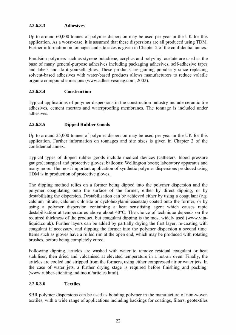
2.2.6.3.3 Adhesives Up to around 60,000 tonnes of polymer dispersion may be used per year in the UK for this application. As a worst-case, it is assumed that these dispersions are all produced using TDM. Further information on tonnages and site sizes is given in Chapter 2 of the confidential annex. Emulsion polymers such as styrene-butadiene, acrylics and polyvinyl acetate are used as the base of many general-purpose adhesives including packaging adhesives, self-adhesive tapes and labels and do-it-yourself glues. These products are gaining popularity since replacing solvent-based adhesives with water-based products allows manufacturers to reduce volatile organic compound emissions (www.adhesivesmag.com, 2002). 2.2.6.3.4 Construction Typical applications of polymer dispersions in the construction industry include ceramic tile adhesives, cement mortars and waterproofing membranes. The tonnage is included under adhesives. 2.2.6.3.5 Dipped Rubber Goods Up to around 25,000 tonnes of polymer dispersion may be used per year in the UK for this application. Further information on tonnages and site sizes is given in Chapter 2 of the confidential annex. Typical types of dipped rubber goods include medical devices (catheters, blood pressure gauges); surgical and protective gloves; balloons; Wellington boots; laboratory apparatus and many more. The most important application of synthetic polymer dispersions produced using TDM is in production of protective gloves. The dipping method relies on a former being dipped into the polymer dispersion and the polymer coagulating onto the surface of the former, either by direct dipping, or by destabilising the dispersion. Destabilisation can be achieved either by using a coagulant (e.g. calcium nitrate, calcium chloride or cyclohexylamineacetate) coated onto the former, or by using a polymer dispersion containing a heat sensitising agent which causes rapid destabilisation at temperatures above about 40°C. The choice of technique depends on the required thickness of the product, but coagulant dipping is the most widely used (www.vita-liquid.co.uk). Further layers can be added by partially drying the first layer, re-coating with coagulant if necessary, and dipping the former into the polymer dispersion a second time. Items such as gloves have a rolled rim at the open end, which may be produced with rotating brushes, before being completely cured. Following dipping, articles are washed with water to remove residual coagulant or heat stabiliser, then dried and vulcanised at elevated temperature in a hot-air oven. Finally, the articles are cooled and stripped from the formers, using either compressed air or water jets. In the case of water jets, a further drying stage is required before finishing and packing. (www.rubber-stichting.ind.tno.nl/articles.html). 2.2.6.3.6 Textiles SBR polymer dispersions can be used as bonding polymer in the manufacture of non-woven textiles, with a wide range of applications including backings for coatings, filters, geotextiles

23

and dishcloths. This application is minor in relation to others relevant for UK industry. The tonnage is included under the section on carpets. 2.2.6.3.7 Foam pillows and mattresses High solids latex is used in the production of foam pillows and mattresses. Synthetic SBR latex is mixed with natural latex and foam is then produced using the Talalay process. Slightly foamed latex mixture is poured into a mould which is partially filled, sealed and the latex expanded under vacuum to completely fill the mould. The temperature is dropped to minus 30°C to freeze the latex, and then carbon dioxide is passed through and the temperature raised to 115 °C to set and vulcanise the foam. Finally the foam block is washed and dried. (www.thesleepcentre.co.uk/dunlopillo.htm, www.vitafoam.co.uk/latex.html) 2.3 TRENDS The technology relating to use of TDM as a chain transfer agent has been in use since the 1950s and is widely reported in the open literature (Cowie, 1991; Urban and Takamura, 2002). It is therefore unlikely that any more cost-effective replacement will be found in the short term. IISRP considers that there is currently no known replacement. Demand for aqueous-based coating and adhesive products is likely to increase due to environmental concerns relating to VOC emissions from solvent-based products, although much change has already occurred in these sectors. Consequently, it can be anticipated that demand for suitable chain transfer agents, including TDM, will also increase. No historical production data have been obtained at this point. 2.4 LEGISLATIVE CONTROLS There are currently no specific legislative controls regulating the use of TDM in the UK or EU.

24

3 ENVIRONMENTAL EXPOSURE The following assessment is based on the methods described in detail in the EU Technical Guidance Document (‘TGD’, EC, 2003), as implemented by the EUSES 2.0 computer program*. The assessment has taken account of site-specific information, and in other respects is generic in that it represents a realistic worst-case. It is, therefore, robust in respect of minor changes in the industry. Further details of the principles and modelling methods can be found in the TGD. A critical assumption made in the environmental exposure assessment is that some residual TDM remains unreacted in products further processed by downstream industry, as discussed in section 2.2.2. Obtaining more measured analytical data may be useful in refining the risk assessment for all life-cycle steps subsequent to emulsion polymerisation. It is certain that products containing any residual TDM will be exported from the UK to other EU member states and beyond. It is equally certain that import of such finished goods will occur. For such a potentially complex issue, a realistic approach is needed. The approach taken is:

1. For the purposes of modelling, assume that imports and exports of finished goods containing residual TDM balance within the present study. In practice, this assumption applies only to the assessment of regional releases from, for example, in-service losses.

2. Review whether the current model calculates any risks from the residual TDM. 3. Refine the model or obtain new data as necessary.

For some stages there is some site-specific information available (described in the Confidential Annex). 3.1 ENVIRONMENTAL RELEASES 3.1.1 General introduction Information on the amount of TDM produced and used in the EU and the UK have been provided by industry, largely on a confidential basis. These data have been used along with the default emission scenarios given in Chapter 3 Appendix 1 (Tables A and B) of the TGD, the ESDs for Plastics Additives (EA, 2003a) and Rubber Additives (UBA, 2003), and the draft ESDs for Pulp, Paper and Board and Paper Recycling (EA, 2002, EA, undated) to develop generic emission scenarios for the different use patterns and life-cycle stages. A full description of the emission scenarios is given in Chapter 2 of the confidential annex. Although the applications of TDM are diverse, the processes used in many of the life-cycle stages are similar and will therefore be grouped together as described in the following sections. EUSES 2.0 has been used to perform the calculations, supplemented with spreadsheet calculations for regional releases where necessary (as outlined in the following sections).

* Available from the European Chemicals Bureau, http://ecb.jrc.it/

25

Information about tonnage is contained within the confidential annex to this report; it is not possible to give anything in this report more detailed than the indicative ranges. Some confidential site-specific release data are available and these are described in Chapter 2 of the confidential annex. 3.1.2 Releases from production There is no production of TDM in the UK, therefore local and regional emissions from production are not applicable to this risk assessment. However, TDM released from production sites could contribute to the continental background concentration (and thereby to the UK) and will thus be assessed on the continental scale. The release rates have been set as equal to those for emulsion polymerisation (section 3.1.3). 3.1.3 Releases from emulsion polymerisation No measured data are available for emissions from emulsion polymerisation. Release rates are therefore based on TGD defaults and expert judgement following a site visit to a major emulsion polymer producer. Due to the strong odour of TDM, high levels of control are in place at sites handling TDM with respect to transfer and storage. It is unlikely that any direct emission of TDM to wastewater takes place, however volatile losses may occur from storage vessels and transfer lines. This view is based on a visit to a typical site. Since the function of TDM is as a reactive intermediate, it is appropriate to refer to the relevant sections of the TGD. From Table A3.3 of the TGD for industrial use, the loss to air is estimated as 0.01%; half of which may be expected to re-condense within the work area and eventually be washed to wastewater. 3.1.4 Releases from a confidential use No measured data are available for emission from the confidential use. Release rates are therefore based on TGD defaults and expert judgement. Releases from this use are estimated as 0.01%, half of which may be expected to re-condense within the work area and eventually be washed to wastewater. This use is discussed further in Chapter 2 of the confidential annex. 3.1.5 Releases from downstream processing As discussed in section 2.2.2, it is likely that trace levels of unreacted TDM remain as residues in solid polymers (up to 2 ppm) and polymer dispersions (up to 100 ppm, wet weight). It can therefore be assumed that there is potential for releases of TDM either as volatile losses or as direct emission to wastewater during the downstream processing of the polymers. The most important sources of potential emissions are summarised in Table 3.1. A full discussion of estimated emissions, including justification of generic site sizes, is provided in Chapter 2 of the confidential annex.

26

Table 3.1 Release of TDM from downstream processing

Life-cycle Stage Type of release Release to air (%) Release to wastewater (%)

Additional solid polymer processing at production sites

Volatile loss 0.125 0.125

Tyre Production Volatile loss 0.06 0.06

Solid Rubber/Polymer Compounding


Solid Rubber/Plastic Goods Production


Carpet and Textile Manufacture Volatile loss and emission to wastewater

1 0.1

Paper Coating Volatile loss and emission to wastewater

1 1

Self-adhesive Labels and Tapes

Volatile loss and emission to wastewater

1 1

Formulation of products adhesives/construction

Volatile loss and emission to wastewater

1 2

Dipping Volatile loss and emission to wastewater

1 2

Foam pillow and mattresses Volatile loss and emission to wastewater

1 0.1

3.1.5.1 Volatile losses No measured data are available for volatile emissions of TDM. Releases are therefore based on defaults described in the ESD for Plastics Additives (EA, 2003a). Volatile losses may occur during downstream processing of polymers containing residual TDM. Releases can be estimated using the compounding and conversion life-cycle stages described in Tables 3.3 and 3.4 of the ESD for Plastics Additives (EA, 2003a), which assume that half is emitted directly to air and the other half re-condenses within the work area and is then washed to wastewater. The ESD is preferred to the TGD as a source of defaults for releases. For a volatile substance, these losses can be summarised as:

Compounding: 0.025% to water; 0.025% to air; Conversion*: 0.125% to water; 0.125% to air; Extrusion: 0.025% to water; 0.025% to air; Calendering: 0.125% to water; 0.125% to air; Injection moulding: 0.025% to water; 0.025% to air.

*open processes, solid articles.

27

The types of process used in further polymer processing at the production site can be considered to be equivalent to “conversion, open processes, solid articles” for a high volatility substance, using Table 3.4 (conversion) of the ESD for plastics additives (EA, 2003a). Emissions are therefore estimated as 0.125% to air and 0.125% to water. For use of polymer dispersions in wet processes, the amount of TDM available for volatilisation is limited by adsorption to suspended polymer particles. On the basis of the partitioning behaviour of TDM between organic matter and water, approximately 1% of the residual TDM has been estimated to be available in the aqueous phase and, as a reasonable worst-case, it could be assumed that all of this would be released to air. 3.1.5.1.1 Tyre production No measured data are available for emissions from tyre production. Release rates are therefore based on defaults described in the ESD for Plastics Additives (EA, 2003a). The processes used in the tyre manufacturing industry are best described by the ESD for plastics additives. The ESD for rubber additives is useful for substances added after polymerisation, but are not helpful for the case of TDM. Creation of the rubber mixture (compounding) is carried out at the same site as tyre production. Emissions from compounding are taken from Table 3.3 (Banbury mixer) of the ESD for plastics additives (EA, 2003a). Handling losses to wastewater would not apply for crumb rubber. Further processing techniques vary dependent on which tyre component is being made. The bulk of the SBR tonnage will be used in treads and side walls (extrusion), with a smaller proportion used in plies and bead wire (calendering). A reasonable split may be 90:10 as an estimate. Emissions are estimated from Table 3.4 of the ESD for plastics additives (EA, 2003a): Compounding: 0.025% to water; 0.025% to air Production: Extrusion (tyre treads and side walls): 0.025% to water; 0.025% to air Calendering (plies and bead wire): 0.125% to water; 0.125% to air Therefore total emissions to each compartment are: 0.025 + 0.9 x 0.025 + 0.1 x 0.125 = 0.06% 3.1.5.1.2 Compounding of solid rubber/polymers No measured data are available for emissions from rubber compounding. Release rates are therefore based on defaults described in the ESD for Plastics Additives (EA, 2003a). The ESD for rubber additives (UBA 2003) does not distinguish between compounding and further processing of rubber into finished goods. However, it is understood that for the UK industry, compounding is often carried out by specialist companies, followed by onward supply to the manufacturers of rubber goods. Releases are estimated as 0.025% to air and 0.025% to water on the basis of Table 3.3 (compounding) of the ESD for plastics additives (EA, 2003a). As for the compounding of rubber mixtures for tyres, handling losses to wastewater would not apply.

28

3.1.5.1.3 Conversion of solid rubber/polymer No measured data are available for emissions from rubber conversion. Release rates are therefore based on defaults described in the ESD for Plastics Additives (EA, 2003a). Table 8 of the ESD for rubber additives suggests that different types of products are manufactured at the same site. However, it is understood from research that the UK industry is fragmented into a large number of specialist companies. The largest typical production volume of a single product type from Table 8 is ca. 5000 kg/d, or 1500 tpa on the basis of 300 days per year. Again, the techniques for conversion of compounded rubber or other polymers into finished articles are best described by the ESD for plastics additives (EA, 2003a). Releases are estimated on the basis of Table 3.4 (conversion), as described for tyre production, but with the addition of injection moulding as a likely process. The split of total tonnage between extrusion, calendering and injection moulding is not known, although it is likely that extrusion and injection moulding are more common. A split of 40:20:40 may be reasonable as an estimate. From Table 3.4: Extrusion: 0.025% to water; 0.025% to air Calendering: 0.125% to water; 0.125% to air Injection moulding: 0.025% to water; 0.025% to air Therefore total emissions to each compartment are: 0.4 x 0.025 + 0.2 x 0.125 + 0.4 x 0.025 = 0.045% 3.1.5.2 Emissions to wastewater Since polymer dispersions are by definition handled in the aqueous form, emissions to wastewater could reasonably be expected to occur from some or all of the following stages in the downstream life-cycle:

− Spillage during transfer of dispersion to storage tanks or blending equipment for compounding;

− Washing-out of used containers; − Spillage during transfer of preparations to application machinery; − Over-spill during application; − Disposal of waste.

3.1.5.2.1 Carpets and textiles No measured data are available for emissions from carpet backing. Release rates are therefore based on expert judgement following a visit to a typical fibre-bonded carpet factory. On the basis of a site visit, emissions to wastewater from carpet and textiles applications is estimated as 0.1% of the latex, due to spillage during transfer and application. Observations were made of typical practice, quantities handled and the amounts of waste processed. This value is lower than the defaults from the TGD, which is 2%, even for the high tonnage used in this application.

29

3.1.5.2.2 Paper coating and self-adhesive tapes and labels No measured data are available for emissions from paper coating and manufacture of self-adhesive tapes and labels . Release rates are therefore based on defaults described in the ESD for Pulp, Paper and Board (EA 2002). From the draft ESD for Pulp, Paper and Board (EA 2002), emissions to wastewater for polymer-based coatings are estimated as 1% of the latex. This release rate is also assumed to apply for application of polymer dispersions to self-adhesive tapes and labels. 3.1.5.2.3 Adhesives and products for the construction industry No measured data are available for emission from use of adhesives and products for the construction industry. Release rates are therefore based on TGD defaults. In the absence of more specific information, a TGD default release rate of 2% of the latex to wastewater is assumed to apply to formulation of inks, and adhesives or products for the construction industry. However, given that latex dispersions form a milky appearance in water even up to very high dilutions, it may be that a waste treatment authority would not allow such high losses. 3.1.5.2.4 Dipping No measured data are available for emission from dipping. Release rates are therefore based on TGD defaults. In the absence of more specific information, a default release rate of 2% to wastewater is assumed to apply to production of dipped rubber goods. However, given that latex dispersions form a milky appearance in water even up to very high dilutions, it may be that a waste treatment authority would not allow such high losses. 3.1.5.2.5 Foam pillow and mattresses No measured data are available for emission from manufacture of foam pillow and mattresses. Release rates are therefore based on TGD defaults. No specific information on release rates is available. However, given the technologies involved, it is assumed that emissions from foam production are similar to those from the carpet backing industry and are therefore emission to wastewater is set at 0.1%. 3.1.5.3 Vulcanisation With the exception of the uses described previously in section 3.1.5.2.3, the final stage of processing of solid rubber and polymer dispersions by downstream industry is vulcanisation, where rubber molecules are cross-linked by curing at the appropriate temperature and pressure. Some further volatile loss of TDM could occur under these conditions.

30

3.1.6 In-service loss Emissions of TDM during the service life of products containing residues are assessed on the regional scale. These are summarised in Table 3.2. 3.1.6.1 Abrasion of tyres Taking the approach used in the draft risk assessment report for tert-4-octylphenol (EA, 2003b), it is estimated that 1 kg of rubber is lost via abrasion of tread compound over the service life of the tyre. This loss is assumed to be distributed evenly between surface water and industrial soil (e.g. roadside verges). Using the estimated residual level of TDM in the rubber used for tyre manufacture, and EU figures for the number of vehicles in use, a regional release of TDM through abrasion can be calculated. The details of this calculation will be retained in the confidential annex until confirmation of residual TDM levels is received from the rubber producers. 3.1.6.2 Use of adhesives and construction products Pre-formulated adhesive and construction products are assumed to be widely distributed to a large number of professional and do-it-yourself users and are therefore unlikely to result in significant local releases. However, overall losses of these aqueous-based products in the region may be relatively high and, in the absence of more specific information, are assumed to be 2% released to water. 3.1.6.3 Service life of other products Table 3.5 of the ESD for plastics additives (EA, 2003a) estimates releases due to leaching to wastewater during the service life of finished articles. This model is used the basis for estimating releases of TDM during the service life of solid polymer articles, carpets, paper products and rubber gloves. Table 3.2, overleaf, sets out how these sources of regional releases are considered in the risk assessment.

31

Table 3.2 Sources of regional releases of TDM from in-service losses Product Description of loss Basis of emission estimate

Tyres Abrasion during use; loss to surface water and industrial soil.

Stockpiled scrap tyres: volatile losses to air

As described in section 3.1.6.1 and confidential annex.

0.01% per year, equivalent to annual loss for outdoor use of solid polymer.

Solid Polymer In-service losses to air and wastewater. Tonnage split 50:50 between indoor and outdoor use.

Service life 5 years.

ESD for plastics additives, volatile substance. 0.05% to air, 0.8% to water for outdoor; 0.05% to air, 0.05% to water for indoor over service life.

Carpet In-service losses to air and wastewater, indoor use.


ESD for plastics additives, volatile substance. 0.05% to air and 0.05% to water over service life.

Paper In-service losses to air.

Service life 1 year.

Equivalent of one year’s worth of emission to air for solid polymer. Emission to wastewater unlikely. 0.01% to air.

Self-adhesive labels and tapes

In-service losses to air.


Equivalent of one year’s worth of emission to air for solid polymer. Emission to wastewater unlikely. 0.01% to air.

Adhesives; construction industry

Losses during application of product. May be used in both professional and do-it-yourself products. Losses to water for aqueous-based products may be important, assumed to be 2%.

Rubber gloves In-service losses to air and wastewater, indoor use.


Equivalent of one year’s worth of emission to air for solid polymer. 0.01% to air and 0.01% to water.

Foam pillows and mattresses

In-service losses to air and wastewater, indoor use.


ESD for plastics additives, volatile substance, 0.05% to air and 0.05% to water over service life.

3.1.7 Releases from disposal 3.1.7.1 End-of-life Tyres There are various options for disposal/recycling of scrap tyres (‘casings’) at the end of their service life, including disposal to landfill, and various forms of recycling/recovery. The Environment Agency reported in 2003 that 480,000 tonnes of tyres go to scrap in the UK each year, approximately equal to 48 million tyres. The majority (300,000 tonnes) is recovered or recycled (the figures have fluctuated around this level since 1999 – UTWG, 2001). 145,000 tonnes were landfilled; in future most of this will need to be disposed of by another route. 16,000 tonnes were used for ‘landfill engineering’ (EA, 2003c). The remaining 19,000 tonnes unaccounted for in the breakdown above may be stockpiled (see below). Garages and tyre retailers pay an estimated £98 million per year for disposal of waste tyres by specially-licensed companies (Scotsman 2003). One of the largest in the UK is the Waste Solution Group, based at Newton Aycliffe.

32

Recycling/recovery The options for recycling/recovery include:

− Energy recovery (i.e. burning as fuel at cement kilns and power stations). − Recycling as crumb (e.g. for use in carpet underlay, and soft shock-absorbing surfaces

such as children’s playgrounds). − Retreading (not believed to be important for car tyres but may be more relevant for

heavy and agricultural vehicles) − Other forms of physical re-use, e.g. underwater reefs (not relevant in UK), use on

farms and as fenders on boats. Presumably, use in landfill engineering would also fall into this category.

(EA, 2003c, Scotsman 2003) The current split between the different recycling/recovery industries is not known. In 1999-2001 data from the Scrap Tyre Working Group (UTWG, 2001) the balance is reported as 8.3-16% for energy recovery, 16.6-22.2% material recycling, 9.9-17% used in retreading and 14.3-16% for physical re-use and 3.3-7.1% for landfill engineering (the remaining tyres were landfilled, illegally dumped or stockpiled). Releases of TDM associated with these processes are not expected to be important.

− Incineration of polymers for energy recovery leads to no releases of polymer additives to air or water from the Emission Scenario Document for polymer additives (EA, 2003a).

− Recycling and retreading processes are expected to be similar to the processes already identified in this risk assessment in respect of carpet underlay production and tyre production respectively and are likely to take place at the same premises. Therefore no additional releases are foreseen.

Landfill and landfill engineering It is no longer legally acceptable for scrap tyres to be disposed of to landfill except at specially licensed sites; shredded tyres can still be landfilled until 2006 at such sites. However, millions of tonnes of scrap tyres will already be in UK landfill sites from disposal prior to the new legislation. Use in ‘landfill engineering’ is assumed to refer to use of the scrap rubber to form a liner layer in the landfill. It is not clear whether this mode of use will be phased out. TDM is highly adsorbing and poorly soluble. These properties indicate that it is highly unlikely to leach from the rubber in landfills. Any loss due to volatilisation would presumably be treated with landfill gas. Coastal defence constructions Collins has published a series of papers on the use of tyres as part of coastal defence constructions, including a review (Collins, 2002a). This review covers uses such as:

• Use in road surfaces in the USA • Use in artificial reef construction in the USA and SE Asia in particular.

The paper cites reviews by other workers in this field, such as Evans (Evans, 1997), as well as those from his own group. Collins' papers (for example, Collins, 2002b) are concentrating on a long-term study in Poole Bay, Dorset. Earlier studies were performed in the laboratory. The balance of evidence from these papers is that:

33

1. There can be uptake of zinc from the tyres into the communities which populate the constructions; PAHs may also be found to leach.

2. Quantities are consistent with leaching from an outer layer of the order of magnitude of a few microns, and that this takes place within a few days of immersion.

3. There is no evidence for other organic compounds leaching, although this would be limited by analytical sensitivity.

In respect of the present project, there is no information to suggest that residual TDM in tyres will leach out into water during this type of use. Any TDM that could leach would already have done so during normal use. Other issues Fly-tipping: The Environment Agency reports that cost of fly-tipping is currently estimated to be over £2 million per year to the Agency, local authorities, emergency services and landowners. There are direct risks to the environment and also economic implications for legitimate recovery industries. (EA, 2003c). In the absence of information it is not possible to estimate the scale of the issue in the UK in respect of quantity of tyres fly-tipped, though the Environment Agency is reported to remove approximately 30,000 tyres per year from UK rivers, and at a particular quarry site in Yorkshire, over 20 million tyres have been illegally dumped over the last 30 years (EA, undated 2). Nevertheless, it can be stated that the properties of TDM indicate that it is highly unlikely to leach from the rubber in fly-tip sites. Stockpiles: The Environment Agency reports that there are large stockpiles of scrap tyres in the UK (13 million tyres, approximately equal to 130,000 tonnes). Such dumps could have risks of fire and pollution of watercourses (EA, 2003c). In respect of the release of TDM specifically, it can be stated that the properties of TDM indicate that it is highly unlikely to leach from the rubber in such stockpiles. Volatile emissions to air contributing to the regional model are theoretically possible and are assumed to be equivalent to outdoor service losses to air for solid polymers. Bacterial reclamation: New technologies for reclamation of rubber from scrap tyres are being sought. One possible new approach, currently under investigation, is the use of specially adapted micro-organisms to break down the tyre and produce pure rubber for recycling (Scotsman 2003). In the future, this could be a viable new mode of recycling. The potential for release of TDM from this process is not known, although microbial degradation may occur. 3.1.7.2 Paper recycling An important proportion of recycled material is utilised by the UK paper-making industry. The draft ESD for paper recycling (EA, undated) indicates that a default of 50% of paper produced in the UK is recycled. Since coated paper such as magazine print is likely to be included in the recycled material, there is potential for local emissions of residual TDM during the recycling process. It could be assumed that this utilisation rate applies for coated paper. Coating chemicals would be released from the paper during the de-inking process and, while TDM may degrade under the conditions of de-inking, as a worst case it is assumed that this is not the case. According to the draft ESD for paper recycling (EA, undated), during the de-inking process, 10% of an insoluble substance is lost to waste water, while 90% is lost to sludge. Sludge from paper recycling may be spread on agricultural land, therefore this needs

34

to be accounted for in the calculation of terrestrial exposure. The SIMPLETREAT defaults are therefore overwritten, assuming that the same proportion of TDM is directed to air, but the remainder is split 90:10 between sludge and water. In the calculation of releases it is assumed that there are 10 recycling sites in the region, and that the water flow rate at them is 8000 m3/day, as described in the ESD for Pulp, Paper and Board (EA 2002). 3.1.7.3 Disposal of other products At the end of service-life, most other articles containing TDM residues are likely to be disposed of either by incineration or landfill. Due to the high adsorption and low solubility, it is unlikely that significant leaching of TDM would occur from landfill sites. Any volatile losses after disposal would be extracted and treated with landfill gas.

35

3.1.8 Summary of emission estimates Tables 3.3 and 3.4 set out the key emissions estimates in kg/d. Regional releases from production, downstream use and service life are summed for the purposes of risk assessment calculations. Table 3.3 Estimated emissions (local and regional) for production and downstream uses

Life cycle stage Compartment Local (kg/d) Regional (kg/d) Continental (kg/d)

Air 0 0 2.05E+00 Production

Water 0 0 2.05E+00

Air 4.17E-02 1.37E-01 1.23E+00 Emulsion Polymerisation Water 4.17E-02 1.37E-01 1.23E+00

Air 1.50E-02 1.23E-02 1.11E-01 Confidential Use

Water 1.50E-02 1.23E-02 1.11E-01

Air 2.83E-04 2.91E-04 2.62E-03 Additional solid polymer processing at production sites Water 2.83E-04 2.91E-04 2.62E-03

Air 1.00E-05 8.22E-05 7.40E-04 Tyre Production

Water 1.00E-05 8.22E-05 7.40E-04

Air 6.25E-06 1.71E-05 1.54E-04 Solid Rubber/Polymer Compounding Water 6.25E-06 1.71E-05 1.54E-04

Air 2.25E-06 3.08E-05 2.77E-04 Solid Rubber/Plastic Goods Production Water 2.25E-06 3.08E-05 2.77E-04

Air 5.33E-03 8.77E-02 7.89E-01 Carpet and Textile Manufacture Water 5.33E-04 8.77E-03 7.89E-02

Air 4.33E-02 1.78E-01 1.60E+00 Paper Coating

Water 4.33E-02 1.78E-01 1.60E+00

Air 7.83E-03 2.58E-02 2.32E-01 Self-adhesive Labels and Tapes Water 7.83E-03 2.58E-02 2.32E-01

Air 1.33E-02 1.37E-02 1.23E-01 Formulation of products adhesives/construction Water 2.67E-02 2.74E-02 2.47E-01

Air 2.92E-03 9.59E-03 8.63E-02 Dipping

Water 5.83E-03 1.92E-02 1.73E-01

Air 1.67E-02 1.37E-02 6.85E-02 Foam pillows and mattresses Water 1.67E-03 1.37E-03 6.85E-03

Air 9E-03 9E-02 8E-01 Paper Recycling

Water 9E-02 8.9E-01 8.0

36

Table 3.4 Estimated emissions (regional) for service life

Life cycle stage Compartment Regional (kg/d) Continental (kg/d)

Industrial Soil Confidential Confidential Tyres

Water Confidential Confidential

Stockpiled tyres Air Confidential Confidential

Air 1.71E-05 1.54E-04 Solid Polymer (Outdoor) Water 2.74E-04 2.47E-03

Air 1.71E-05 1.54E-04 Solid Polymer (Indoor) Water 1.71E-05 1.54E-04

Air 4.38E-03 3.95E-02 Carpet

Water 4.38E-03 3.95E-02

Air 1.78E-03 1.60E-02 Paper

Water 0 0

Air 2.60E-04 2.34E-03 Self-adhesive labels and tapes Water 0 0

Air 0 0 Adhesives; construction industry Water 2.74E-02 2.47E-01

Air 9.59E-05 8.63E-04 Rubber gloves

Water 9.59E-05 8.63E-04

Air 6.85E-04 2.74E-03 Foam pillows and mattresses Water 6.85E-04 2.74E-03

37

3.2 ENVIRONMENTAL FATE AND DISTRIBUTION 3.2.1 Atmospheric degradation No measured data are available. TDM released to the atmosphere is likely to be rapidly degraded by reaction with hydroxyl radicals. The rate constant for this fate process has been estimated using the AOP program (v1.91) as 43.5E-12 cm3.molecule-1.s-1 (Industry IUCLID, MTC, 2003). From this rate constant the estimated half-life for the reaction of hydroxyl radicals with TDM in the atmosphere was calculated as being 2.95 hours (assuming 1.5 million hydroxyl radicals per cm3). The rate constant for reaction of 2,2,4,6,6-pentamethyl-4-heptanethiol with hydroxyl radicals was estimated to be 36.5E-12 cm3.molecule-1.s-1 using AOPWIN v1.91 (SRC, 2000), as shown in Appendix 1. From this rate constant the estimated half-life for the reaction with hydroxyl radicals in the atmosphere is calculated as being 1.58 days, assuming an average concentration of 5E+05 hydroxyl radicals per cm3, according to the TGD default. Measured rate constants for methanethiol and ethanethiol are reported in the literature as 25.6E-12 and 31.6E-12 cm3.molecule-1.s-1 respectively (Lee and Tang, 1983). These values are consistent with the AOPWIN predictions. 3.2.2 Aquatic degradation The potential for degradation of TDM is crucial for determining if the PBT criteria are met, as well as being important in the calculation of exposure concentrations. Although oxidation of the thiol is possible in principle, as discussed below, on the basis of the available information, a definitive conclusion cannot be reached regarding persistence in the environment. A more detailed discussion of the degradation of TDM is given in Appendix 4. 3.2.2.1 Abiotic degradation No experimental abiotic degradation data are available for TDM. Based on chemical structure, it can be assumed that TDM is not susceptible to abiotic degradation by hydrolysis. Abiotic degradation of thiols to disulfides or sulfonic acids by oxidation is reported in literature (e.g. Patai, 1974, March, 1992; Giles et al, 1986). Under laboratory conditions, mild oxidants (including oxygen in both gas and solution phases), convert thiols first to disulfides. A reactivity order: primary SH > secondary SH > tertiary SH has been observed, with an approximately 10 fold difference for isomeric thiols. In aqueous solution, catalysis by base is observed. Prolonged exposure to the same reagents lead eventually to sulfonic acids. It is not known, however, whether this route is applicable under environmental conditions i.e. high dilution. (Pers. Comm., Ian Watts, University of Manchester, December 2004). In aqueous solution, the reaction can be catalysed by transition metals such as copper, manganese and iron (Bagiyan et al, 2003; Smith et al, 1994). Chemists using oxidation as a synthetic route in the laboratory reported that this is difficult for TDM, requiring harsh experimental conditions (Pers. Comm, Feb 2004). However, the methods used are not relevant to environmental conditions (i.e. high dilution in aqueous solution). In an algal toxicity test conducted by the Japanese National Institute for Environment Studies (described in the confidential annex), significant decreases in TDM test concentrations were observed over the study period. Further investigation of these losses was carried out and it

38

was concluded that that degradation was caused by oxidation in air. However, the evidence for oxidation of TDM under environmental conditions is not conclusive. A new study of the abiotic degradation of TDM in aerated solution would help to resolve whether TDM is oxidised in the environment. For the purposes of this assessment, it is assumed that TDM does not oxidise under environmental conditions. Within the polymer (P-S-R, where R is the TDM backbone), oxidation of sulfur to sulfone and then to a sulfonate, where the sulfonate could presumably be left attached to P or R could occur. In the latter case oxidised TDM would be formed. These reactions do not appear to readily occur. In the short term, for some applications, they would be very unlikely due to the extensive use of antioxidants by rubber producers and processors. It seems unlikely that polymer degradation could release TDM at a rate that it is realistic to estimate. 3.2.2.2 Biodegradation TDM attained 10.4% degradation in 28 days in a non-GLP ready biodegradation test conducted according to test guideline OECD 301D (Elf Atochem, 1994). This study is assigned reliability 2 and is reviewed in detail in Appendix 5. Results of 0% degradation in a further two non-GLP tests conducted according to OECD 301D are also reported in the industry IUCLID (ATOCHEM, 1990; Bayer AG internal study, 1973). It is not possible to assess the reliability of these studies without reviewing the original reports. On the basis of the available data, TDM is considered to be not readily biodegradable. 3.2.3 Degradation in soil No experimental data are available on the degradation of TDM in soil. 3.2.4 Evaluation of environmental degradation data There is no compelling evidence that degradation in the sewage treatment system or the environment can be allowed for in the assessment. Hence, all rate constants for biodegradation are set to zero. 3.2.5 Environmental partitioning According to calculations using a Mackay level III fugacity model, TDM will, after release to a specific environmental compartment, distribute in the environment as in Table 3.5 (CEMC, 2002). The input parameters used for this modelling are those given in Table 1.1.

39

Table 3.5 Environmental distribution of TDM

Mass % Compartment

Release to air only Release to water only Release to soil only

Air 99.9 0.036 1.66

Water 2.9 x 10-4 9.53 0.011

Sediment in water 2.7 x 10-3 90.4 0.11

Soil 0.11 4 x 10-5 98.2

These results indicate a general lack of movement between compartments, due to high affinity for both air and solids. 3.2.6 Adsorption No measured log Koc value is available for TDM. Using the QSAR for predominantly hydrophobics from the TGD (log Koc = 0.81 log Kow + 0.1), a log Koc value of >5.12 can be calculated from the measured log Kow value of >6.2. A log Koc value of 3.50 (Koc = 3.18E+03) was estimated using the PCKOCWIN v1.66 for 2,2,4,6,6-pentamethyl-4-heptanethiol (SRC, 2000), as shown in Appendix 1. The following partition coefficients have been calculated using EUSES 2.0 from the log Koc value of 5.12: Kpsusp 1.33 x 104 l/kg Partition coefficient for solids/water in suspended matter Kpsed 6.6. x 103 l/kg Partition coefficient for solids/water in sediment Kpsoil 2.65 x 103 l/kg Partition coefficient for solids/water in soil Ksoil-water 4.01 x 103 Soil/water partitioning coefficient Ksusp-water 3.31 x 103 Suspended matter/water partitioning coefficient Ksed-water 3.31 x 103 Sediment/water partitioning coefficient The sewage treatment plant model used in EUSES 2.0 estimates the fraction of a substance entering the works that will be directed to air, water and sludge. For TDM the fractions are: air 0.234; water 0.0454; and sludge 0.720. In practice, using the lower log Koc value of 3.5 would not change the overall conclusions of the assessment. Using this value, the SIMPLETREAT model within EUSES 2.0 predicts 75.4% to air, 4.2% to water and 20.3% to sludge. PEC/PNECs for the aquatic and sediment compartments would remain virtually unchanged, while the values for the terrestrial compartment would be a factor or around 3.5 lower due to the smaller fraction being spread on agricultural land. 3.2.7 Volatilisation The volatilisation of TDM from surface water to air may be estimated from the Henry’s Law Constant. This has been calculated as 4.27E+05 Pa.m3.mol-1 (see Section 1.3.9.2). An air-water partitioning coefficient (Kair-water) may be derived from the Henry’s Law Constant and is calculated as 180.2 m3.m-3. The Kair-water and Henry’s Law Constant are high, indicating

40

that volatilisation is a potential removal mechanism from water. EUSES 2.0 accounts for this in all compartments other than local water. 3.2.8 Precipitation The high adsorption coefficient suggests that some TDM found in the atmosphere may adsorb to particulate matter, which may then be washed out by rainfall. 3.2.9 Bioaccumulation and metabolism A BCF of 3.8 x 104 was calculated for fish using EUSES 2.0 with the log Kow of >6.2 and the following TGD equation for substances with a log Kow of >6 (this equation is based on a parabolic relationship in fish developed by Connell and Hawker, 1988): log BCFfish = –0.20 * (logKow)2 + 2.74 * logKow – 4.72 A BCF of 1.9 x 104was calculated for earthworms using EUSES 2.0. 3.2.10 Environmental properties of predicted oxidation products 3.2.10.1 Disulfides According to the literature, as discussed in section 3.2.2.1, disulfides are obtained following oxidation of thiols under laboratory conditions. No measured data are readily available for tert-dodecyldisulfide, therefore the QSAR predictions were obtained using EPIWIN v. 3.12. The key environmental properties are summarised in table 3.6. The full EPIWIN output is given in Appendix 1. The disulfide is expected to be recalcitrant in the environment and potentially bioaccumulative. It may not, however, exhibit toxicity to aquatic organisms up to its limit of solubility. In practice, concentrations of TDM discharged to the environment at all stages of the life cycle are so low that dimerisation is unlikely.

41

Table 3.6 Predicted properties of tert-dodecyldisulfide

Property Value

Vapour pressure (Pa) 3.56E-04

Water solubility (mg/l) from log Kow 1.62E-07 (4.3E-04)*

Water solubility (mg/l) fragment method 4.18E-06

log Kow 12.01

BIOWIN 1 -0.5478 Does not biodegrade fast

BIOWIN 2 0.0000 Does not biodegrade fast

BIOWIN 3 (ultimate) 1.0363 Recalcitrant

BIOWIN 4 (primary) 2.3460 Weeks-months


Biodegradation


*Fish LC50 (mg/l) 6.8E-04

*Daphnia EC50 (mg/l) 1.1E-03

*Algal EC50 (mg/l) 9.8E-04 * Value obtained setting log Kow = 8 (maximum realistic value) 3.2.10.2 Sulfonic acids Sulfonic acids are theoretically the ultimate oxidation products of thiols following prolonged exposure to mild oxidising conditions. Under environmental conditions and at dilute concentrations, it is possible that TDM may oxidise to sulphonic acids. No measured data are readily available for tert-dodecylsulfonic acid, therefore QSAR predictions were obtained using EPIWIN v. 3.12. The key environmental properties are summarised in table 3.7. The full EPIWIN output is given in Appendix 1. The sulphonic acid is predicted to have moderately high water solubility and the predicted log Kow does not indicate significant bioaccumulation potential, although it is not likely to be rapidly biodegraded in the environment. The sulfonic acid is not expected to be harmful to aquatic organisms, although it will have surfactant properties.

42

Table 3.7 Predicted properties of tert-dodecylsulfonate

Property Value

Vapour pressure (Pa) 2.01E-04

Water solubility (mg/l) from log Kow 119.4

Water solubility (mg/l) fragment method 27692

log Kow 2.69


BIOWIN 2 0.7533 Biodegrades fast

BIOWIN 3 (ultimate) 2.2021 Months

BIOWIN 4 (primary) 3.2033 Weeks


Biodegradation


Fish LC50 (mg/l) 417

Daphnia EC50 (mg/l) 469

Algal EC50 (mg/l) 305 3.2.11 Summary of environmental fate and distribution The available data indicate that TDM is highly volatile, although it is moderately adsorbing and has low solubility in water. It can be expected to volatilise from water and adsorb to organic matter in sediments, soils and sludges. Degradation via biotic processes is expected to be slow. Atmospheric degradation through reaction with hydroxyl radicals is expected to occur rapidly. The available evidence for oxidation of TDM under environmental conditions is not conclusive. TDM is considered to have a high potential to bioaccumulate in aquatic organisms.

43

3.3 ENVIRONMENTAL CONCENTRATIONS 3.3.1 Aquatic compartment (surface water, sediment and wastewater

treatment plant) 3.3.1.1 Estimated aquatic environmental concentrations The predicted environment concentrations (PECs) for water local to the point of release (PEClocal) are calculated using the environmental releases detailed in Section 3.1 and the equations set out in Chapter 3 of the Technical Guidance Document. The local PEC is the sum of a local water concentration (Clocal) resulting from the relevant process emission, and a background concentration that results from emissions in the regional environment (PECregional). The sewage effluent low flow rate is assumed to be 2000 m3/d for all life-cycle stages other than paper recycling, where a low flow rate of 8000 m3/d is applied. The dilution factor for discharge to river is assumed to be 10. Site-specific data are available for some life-cycle stages and these are given in Chapter 2 of the confidential annex. The marine compartment is assessed in a similar way. However, the possibility of release from use directly into the sea is allowed for, with a dilution of 100. The PEC for sediment can be derived from the PEClocal for surface water using the suspended matter-water partitioning coefficient, assuming equilibrium partitioning, as described in the TGD. The results are presented in Tables 3.8 and 3.9 Table 3.8 Overall regional and continental aquatic PECs

PECs for surface water(mg/l) PECs for sediment (μg/kg wet wt)

Scale

Freshwater (dissolved) Marine Freshwater Marine

Regional 5.01E-7 4.82E-8 2.88 0.274

Continental 6.67E-8 1.06E-10 0.382 6E-4

44

Table 3.9 Local aquatic PECs

Freshwater Marine Life-cycle stage

PECaquatic (mg/l)

PEC sediment (mg/kg wet

weight)

PECaquatic (mg/l)

PEC sediment (mg/kg wet

weight)

PECs for WWTP

organisms (mg/l)

Emulsion Polymerisation 7.94E-5 0.229 1.74E-4 0.501 9.46E-4

Confidential Use 2.89E-5 0.0834 6.26E-5 0.18 3.41E-4

Additional solid polymer processing 1.04E-6 2.99E-3 1.23E-6 3.54E-3 6.44E-6

Tyre Production 5.2E-7 1.5E-3 8.25E-8 2.59E-4 2.27E-7


5.13E-7 1.48E-3 7.43E-8 2.14E-4 1.42E-7


5.06E-7 1.46E-3 5.76E-8 1.66E-4 5.11E-8

Carpet andTextile Manufacture 1.51E-6 4.36E-3 2.27E-6 6.55E-3 1.21E-5

Paper Coating 8.26E-5 0.238 1.81E-4 1.49E-4 9.84E-4

Self-adhesive Labels and Tapes 1.53E-5 0.0442 3.27E-5 0.0943 1.78E-4


5.1E-5 0.147 1.11E-4 0.321 6.06E-4

Dipping 1.16E-5 0.0333 2.44E-5 0.0703 1.32E-4

Foam pillows and mattresses 3.66E-6 0.0105 7E-6 0.0202 3.79E-5

Paper Recycling 4.33E-5 0.125 9.42E-5 0.271 5.13E-4

3.3.1.2 Measured aquatic environmental concentrations The Environment Agency has collected sediment monitoring data for TDM in eight regions: North East, North West, Midlands, Anglian, South West, Thames, and Southern, and Wales (EA, 2004). The samples were taken between January and April 2003. Samples were collected as part of the Chemical Strategy Pilot Monitoring Programme; they were not taken specifically for this assessment. The results are summarised in Table 3.10 below. The majority of results are <2500 µg/kg, presumably the limit of detection. Only three results over all eight regions are above this. The highest concentration recorded is 5500 µg/kg. Some potential weaknesses are known to exist within this data set, in that the nature of the analytical method means that it is possible for false positive or high results to be recorded. The analysis involves extraction of the sediment with solvent and then analysing the extract on a gas chromatograph fitted with an atomic emission detector set in sulfur mode (a highly selective detector for measuring sulfur-containing compounds) (Pers. comm. 02/06/04). The

45

calibration standard is a mixture of C9-C14 tertiary alkylthiols, which gives a recognisable pattern (Pers. comm. 25/05/04). The presence of the compounds is indicated by this pattern together with the retention time, and the quantitation is worked out by summing the peaks in the chromatogram. However, for some sediments the supposedly recognisable pattern altered, presumably due to some of the compounds being retained on the sediment more than others. Using this method, the potential appears to exist for other sulfur compounds present to be detected, giving a false positive or high result. The results are correct based on a technical mixture of alkylthiols and not true reference materials (Pers. comm. 02/06/04); however any ‘rogue’ positive substances can be said to be sulfur-containing substances with the same retention time as the TDM components. Table 3.10 Summary of Environment Agency sediment monitoring data

Region Timescale Number of sampling sites

Total number of results reported

Range of results

North East All 18/03/03 3 7 <2500 µg/kg – ‘No result’1

North West 31/01/03 – 04/04/03 2 12 <2500 µg/kg – 5500 µg/kg 2

Midlands 24/02/03 – 31/03/03 2 6 All <2500 µg/kg

Anglian 11/03/03 – 28/03/03 2 6 <2500µg/kg

South West 17/03/03 – 25/03/03 2 6 All <2500 µg/kg

Thames All 10/03/03 2 5 <2500 µg/kg – 4340 µg/kg 3

Southern All 06/03/03 2 6 All <2500 µg/kg

Wales 07/03/03 – 21/03/03 2 6 All <2500 µg/kg Notes 1 Presumably a failed analysis rather than a zero reading. 2 Two positive results: recorded at Manchester Ship Canal, upstream of Irlam Locks (3680 µg/kg) and Douglas at Wanes Blades Bridge (5500 µg/kg). 3 One positive result: recorded at South Marston Brook at Nightin (4340 µg/kg). NB. Samples taken later the same day at the same sample point give <2500 µg/kg. 3.3.1.2.1 Comparison of measured and estimated aquatic concentrations The potential exists for the measured values to be falsely high or positive, as described above, and as such, should not be used as the basis of any risk characterisation. However, to give an indicative preliminary view, the values can be compared against PEC for the appropriate scale – continental or regional background, or local PEC. The locations for sampling were recommended by local Environment Agency offices, and it is believed that the locations were selected because they are associated with industrial activity involving alkylthiols. Therefore it is likely that the samples could represent a local concentration. The detection limit is much higher than the PEC values obtained by modelling; the highest of which is around 9 µg/kg. Some values above the detection limit were found. It is not considered realistic to interpret these results in detail, but it is important to follow up those

46

locations to find out more about the industrial source of the contamination and whether there are regular releases of TDM. 3.3.2 Terrestrial compartment 3.3.2.1 Estimated soil concentrations The TGD method takes into account direct releases to soil, application of sewage sludge containing the chemical and atmospheric deposition. For TDM no direct releases to soil are expected. Three different soil PECs can be calculated depending on the protection goal: natural soil (PECnat,soil), agricultural soil (PECagr,soil) and grassland (PECgrassland). These vary in terms of the depth of soil considered and the duration/route of exposure. The 30-day average for agricultural soil represents the PECs for soil organisms, while the 180-day average for grassland represents exposure to animals through the food chain. At the regional level the soil concentration in unpolluted or “natural” soil must be used as the background concentration, in order to avoid double-accounting of application through sludge. Regional and continental terrestrial PECs for TDM are provided in Table 3.10. The local PECs for the terrestrial compartment are given in Table 3.12. 3.3.2.2 Measured soil environmental concentrations No measured data are available for concentration of TDM in soil. 3.3.3 Atmospheric compartment Releases to air have been calculated, but in the absence of any specific effects in air these are not discussed further.

47

Table 3.11 Overall regional and continental terrestrial PECs

Scale PEC for agricultural soil (mg/kg wet weight)

PEC porewater (mg/l)

Regional 6.02E-4 2.56E-7

Continental 7.15E-5 3.04E-8

Table 3.12 Local terrestrial PECs

Life-cycle stage PEC for agricultural soil (30 days)

(mg/kg wet weight)

PECs grassland (180 days)

(mg/kg wet weight)

PEC porewater (agricultural soil)

(mg/l)

Emulsion Polymerisation 0.0167 5.79E-4 1.23E-6

Confidential Use 6E-3 2.09E-4 4.42E-7

Additional solid polymer processing

1.13E-4 3.94E-6 8.34E-9

Tyre Production 4E-6 1.4E-7 2.95E-10


2.5E-6 8.74E-8 1.84E-10


9.01E-7 3.18E-8 6.64E-11

Carpet andTextile Manufacture 2.13E-4 7.45E-6 1.57E-8

Paper Coating 0.0173 6.02E-4 1.28E-6


3.13E-3 1.09E-4 2.31E-7


0.0107 3.71E-4 7.85E-7

Dipping 2.33E-3 8.11E-5 1.72E-7

Foam pillows and mattresses 6.67E-4 2.33E-5 4.91E-8

Paper Recycling 9.03E-3 3.14E-4 6.64E-7

48

3.3.4 Food chain exposure 3.3.4.1 Estimated environmental concentrations PECs for secondary poisoning are presented in Table 3.13. Table 3.13 PECs for secondary poisoning

Life-cycle stage PECs for fish eaten by predators

(mg/kg wet weight)

PECs for marine fish eaten by

predators (mg/kg wet

weight)

PECs for marine top predators (mg/kg wet

weight)

PECs for worms eaten by predators

(mg/kg wet weight)

Emulsion Polymerisation 12.5 27.2 54.5 0.0128

Confidential Use 4.63 9.79 19.7 6.05E-3


0.275 0.203 0.553 2.29E-3

Tyre Production 0.194 0.0248 0.196 2.22E-3


0.193 0.0224 0.191 2.22E-3


0.191 0.0198 0.186 2.22E-3

Carpet andTextile Manufacture 0.349 0.366 0.878 2.36E-3

Paper Coating 13 28.3 56.7 0.0133

Self-adhesive Labels and Tapes 2.51 5.12 10.4 4.22E-3


8.08 17.4 34.9 9.02E-3

Dipping 1.92 3.82 7.79 3.71E-3

Foam pillows and mattresses 0.684 1.1 2.36 2.65E-3

Paper Recycling 8.21 17.7 35.5 7.98E-3

3.3.4.2 Measured environmental concentrations in biota No measured data for concentrations of TDM in biota are available.

49

3.4 MARINE EXPOSURE ASSESSMENT The marine PECs are calculated by EUSES 2.0 using the methods given in the Technical Guidance Document. TDM does not contain any ionisable functional groups, therefore the partition coefficients derived for the freshwater assessment can be used without adjustment. TDM is not significantly biodegradable on the basis of freshwater tests, therefore it is considered to be persistent in the marine environment. For the local assessment it is assumed that industrial effluents are not treated in a municipal biological STP and a dilution factor of 100 can be assumed for discharges to coastal regions. Values of PECregional(seawater), Clocal seawater, PEClocal(seawater) and PEClocalsed are evaluated in accordance with the revised TGD. PECs for the marine environment are reported in Tables 3.6 and 3.7 with the freshwater PECs. Secondary poisoning PECs for marine predators are presented in table 3.11 together with the freshwater data.

50

4 EFFECTS ASSESSMENT: HAZARD IDENTIFICATION AND DOSE (CONCENTRATION) - RESPONSE (EFFECT ASSESSMENT)

The following Sections review the available toxicity data for tertiary-dodecanethiol with aquatic and terrestrial organisms. A reliability assessment is given for each study (this appears in the summary Tables within each Section). The assessment is based on the Klimisch system, which includes the following categories:

1 Reliable without restriction. “studies or data…generated according to generally valid and/or internationally accepted testing guidelines (preferably according to GLP) or in which the test parameters documented are based on a specific (national) testing guideline….or in which all parameters described are closely related/comparable to a guideline method.”

2 Reliable with restrictions. “studies or data….(mostly not performed according to GLP), in which the test parameters documented do not totally comply with the specific testing guidelines, but are sufficient to accept the data or in which investigations are described which cannot be subsumed under a testing guideline, but which are nevertheless well documented and scientifically acceptable.”

3 Not reliable. “studies or data….in which there were interferences between the measuring system and the test substance or in which organisms/test systems were used which are not relevant in relation to the exposure (e.g., unphysiologic pathways of application) or which were carried out or generated according to a method which is not acceptable, the documentation of which is not sufficient for assessment and which is not convincing for an expert judgement.”

4 Not assignable. “studies or data….which do not give sufficient experimental details and which are only listed in short abstracts or secondary literature (books, reviews, etc.).”

With the exception of one acute Daphnia test, the assessment of the reliability of the tests and assignment of the relevant Klimisch codes was performed by NIES (National Institute for Environmental Studies, Japan) or the compilers of the IUCLID entries, as indicated in Table 4.1. In terms of the risk assessment, toxicity data assigned a reliability assessment of 1 or 2 will be considered in preference to the other toxicity data when deriving the PNEC. 4.1 AQUATIC COMPARTMENT (INCLUDING SEDIMENT) The results of toxicity tests carried out with tertiary-dodecanethiol on fish (acute), aquatic invertebrates (acute and chronic), and algae (acute/chronic) have been collated from IUCLID, from a Material Safety Data Sheet (MSDS), from an original report and from summary reports provided by the Japanese National Institute for Environment Studies (NIES). The data are summarised below and in Table 4.1. The original sources of most of the test data contained in IUCLID and the MSDS could not be reviewed because the sponsors of the tests did not make them available. Consequently an independent assessment of the reliability of these test data could not be made. The report of an acute Daphnia test was however reviewed (see Appendix A5.2) and an independent assessment made of its reliability. Robust study summaries provided by NIES were reviewed

51

and an assessment of the reliability of these data made. The full summaries are included in Chapter 4 of the confidential annex. 4.1.1 Toxicity to fish 4.1.1.1 Acute toxicity Acute toxicity data are reported in IUCLID and in a Material Safety Data Sheet (MSDS) for three fish species: Brachydanio rerio (Zebrafish), Leuciscus idus (Golden orfe) and Salmo salar (Salmon). The lowest reported LC50 value of 0.9 mg/l was for Salmo salar. This value did not have a reliability assessment in IUCLID and was slightly above the pure water solubility of the substance (0.25 mg/l). Toxic effects were observed in the test with Leuciscus idus (LC50 between 50 and 100 mg/l) but again the result is above the water solubility and the result was assessed as being unreliable in IUCLID. The reliability assessment of 2 given in IUCLID for the B. rerio LC0 of >10000 mg/l does not appear to be appropriate given that the value is so much greater than the solubility of the substance. In a flow-through test with Oryzias latipes (NIES), conducted to GLP according to OECD 203, a 96 hour LC50 of 0.377 mg/l was reported. The test was assigned a reliability code of 2. However, test concentrations included some that exceeded the water solubility of the substance. Analysis of the test media confirmed the presence of concentrations above water solubility in fresh and old media, although this may have been a consequence of use of a dispersant to prepare the test solutions. Concentration-dependent effects were observed. The full study summary is included in the confidential annex. In the absence of a definitive value, but in the presence of observed toxicity in the tests with L. idus, and O. latipes an LC50 equal to the water solubility of 0.25 mg/l has been set for the purposes of risk assessment. This value would need to be reviewed should more reliable data become available. 4.1.1.2 Chronic toxicity No chronic toxicity data are available for fish. 4.1.2 Toxicity to aquatic invertebrates 4.1.2.1 Acute toxicity Acute toxicity data are reported in IUCLID for two invertebrate species: Daphnia magna and a Ceriodaphnia species. A study report for one of these tests was made available for review. Additional data for D. magna were obtained from an MSDS. EC50 values ranging between 0.16 and 3.9 mg/l are reported in IUCLID and in the MSDS. Values above the water solubility of the substance are considered unreliable even though they may have been assigned reliability 1 or 2 in IUCLID. The results of one test (Elf Atochem a) have been reinterpreted following review of the test report to take into account decreases in concentration of the test substance. This has resulted in a recalculated EC50 of 0.068 mg/l and

52

a reassignment of reliability 1 (from 2) to the result. Further information is given in Appendix 5. In a GLP study conducted according to OECD 202 (NIES) an EC50 of 0.0178 mg/l was reported, based on mean measured concentrations, and was assigned a reliability code of 1. Test solutions were prepared using DMSO at a concentration of 100 µl/l. The full study summary is included in the confidential annex. Significant concentration losses were observed in this test. 4.1.2.2 Chronic toxicity A 21-day Daphnia reproduction study was conducted to GLP according to OECD 211 (NIES), and was assigned a reliability code of 1. Significant concentration losses were observed in the test. A NOEC of 0.0108 mg/l was reported based on time-weighted mean measured concentrations. Test solutions were prepared using DMSO at a concentration of 100 µl/l. The coefficient of variation for reproduction in the controls was 6.4% for solvent controls and 11% for normal controls. This is well within the OECD validity criterion of < 25%. The full study summary is included in the confidential annex.

4.1.3 Toxicity to algae

Data are reported in IUCLID and in an MSDS from two tests with one species of algae, Scenedesmus subspicatus. The tests gave 72 h EC50 values of 81 and >100 mg/l. Both results are significantly above the water solubility of the substance and undissolved test material was observed on the walls of test vessels. They aretherefore considered unreliable even though they are assigned reliability 1 in IUCLID. One of the tests also determined an EC10 of 52 mg/l but this is again viewed as being unreliable because it is above the water solubility of the substance. An algal inhibition study was conducted to GLP (NIES, see confidential annex) according to OECD 201 with Selenastrum capricornutum. The test was assigned a reliability code of 3 (invalid) since difficulties in maintaining exposure concentrations made the result unreliable. Further investigation of these losses was carried out and it was concluded that that degradation was caused by oxidation in air. Given the high initial starting concentrations (up to 33.3 mg/l), and the absence of observed effects, it can be concluded that the substance is unlikely to be toxic to algae following short-term exposure. The full study summary is included in the confidential annex. It is concluded that there are no reliable toxicity data for algae that can be used to derive a PNECaquatic. 4.1.4 Toxicity to microorganisms Data are reported in IUCLID for toxicity tests conducted with two single species cultures of bacteria (Pseudomonas putida and Pseudomonas florescens) and with an activated sludge culture. The EC50 values (reliability 2 in IUCLID) determined for P. putida and activated sludge were both >10000 mg/l. Similarly the EC0 value determined for P. florescens

53

(reliability 3) was also >10000 mg/l. (Note: It is normal practice to conduct these tests at concentrations exceeding the water solubility of the test substance (0.25 mg/l in this case) and express the results relative to nominal exposure concentrations). 4.1.5 Toxicity to amphibians No data are available for amphibians. 4.1.6 Toxicity to sediment-dwelling organisms No data are available and therefore a PNEC for sediment is derived by the equilibrium partitioning method and compared with the PEC values for sediment.

54

Table 4.1 Toxicity of TDM to aquatic organisms (ND = no data) Test species Test protocol Year test

completed Endpoint and exposure period

Result (mg/l)1 Reliability assessment2

Comments Study reference

Toxicity to fish Brachydanio rerio (Zebrafish)

Method proposed by the German Federal Environmental Agency (UBA): mainly equivalent to the OECD 203

1992 96-h LC0

>10000 (N) 2(a) Static test. IUCLID entry notes that undissolved particles remained on the surface of the test medium as an oil layer. The test concentration was significantly greater than the reported water solubility of the substance (0.25 mg/l).

IUCLID entry

Leuciscus idus (Golden orfe)

Determination of Acute Toxicity to fish (German Working Group "Fish test" designed especially for detergents)

1973 48-h LC0 48-h LC100

50 (N) 100 (N)

3(a) Static test. IUCLID entry notes that documentation was insufficient for assessment. Results exceed the water solubility of the substance (0.25 mg/l).

IUCLID entry/MSDS

Salmo salar (Salmon)

Not reported in IUCLID Not reported in IUCLID

LC50 0.9 (N) Not reported in IUCLID

Static test. Result exceeds the water solubility of the substance (0.25 mg/l).

IUCLID entry

Oryzias latipes (Medaka)

OECD 203 2000 96-h LC50 0.377 2(c) Result exceeds the water solubility of the substance (0.25 mg/l).

NIES

Toxicity to aquatic invertebrates

Daphnia magna OECD 202 2000 48-h EC50 0.0178 2(c) Results based on measured concentrations. NIES Daphnia magna OECD 211 2000 21-d NOEC 0.0108 1(c) Results based on time-weighted mean

concentrations. NIES

Daphnia magna (Cladocera)

OECD Guideline 202 1997 48-h EC50 0.16 (M - Measured initial concentration) 0.068 (M -geometric mean measured concentration)

2(a) 1(b)

Static test. IUCLID reports the test result in terms of the initial measured concentrations of the substance in the test media. A reinterpretation of the results based on the likely geometric mean concentrations throughout the test period would suggest that a more representative 48-h EC50 value would be 0.068 mg/l. This value is still likely to be an overestimate of the true EC50 value because analysed exposure concentrations in the lowest treatments were below the limit of quantitation and in some cases below the limit of detection of the analytical method. A reliability assessment for the study of 1 is considered more appropriate.

IUCLID entry Test report


Directive 84/449/EEC, C.2: Acute toxicity for Daphnia

1999 48-h EC50

>0.25 (N)

2(a) Static test. IUCLID reports the result as an EC50, it is more likely to be a NOEC since only one

IUCLID entry

55

Test species Test protocol Year test completed

Endpoint and exposure period



concentration was tested. Daphnia magna (Cladocera)


48-h EC0 48-h EC50 48-h EC100

0.05 (N) 0.29 (N) approx. 1.1 (N)

4(a) Static test. Results exceed the water solubility of the substance (0.25 mg/l).

IUCLID entry


Not reported in MSDS Not reported in MSDS

48-h LC50 0.598 4(b) No details of test reported in MSDS. Result exceeds the water solubility of the substance (0.25 mg/l).

MSDS


Method proposed by the German Federal Environmental Agency (UBA): Daphnia Immobilisation Test

1989 24-h EC0 24-h EC50 24-h EC100

1.4 (N) 3.9 (N) 11 (N)

1(a) Static test. IUCLID entry notes that oily droplets were present in the test media. Results exceed the water solubility of the substance (0.25 mg/l).

IUCLID entry


Directive 84/449/EEC, C.2: Acute toxicity for Daphnia

1999 48-h EC50

>0.25 (N)

2(a) Static test. IUCLID reports the result as an EC50, it is more likely to be a NOEC since only one concentration was tested.

IUCLID entry



24-h EC50 1.4-24 (N) Not reported in IUCLID

Static test. Result exceeds the water solubility of the substance (0.25 mg/l).

IUCLID entry

Cereodaphnia sp. (Cladocera)

Not reported in IUCLID 1991 (Date of results publication)

48-h EC50 <0.5 (N)

2(a) Static test. IUCLID entry

Toxicity to algae Scenedesmus subspicatus (Freshwater alga)

Method DIN 38412, Teil 9, of German Standards Institution

1990 72-h EC10 72-h EC50

52 (N) >100 (N)

1(a) The test was not supported by analysis of exposure concentrations. Result exceeds the water solubility of the substance (0.25 mg/l).

IUCLID entry

Scenedesmus subspicatus (Freshwater alga)

Method DIN 38412, Teil 9, of German Standards Institution

1990 72-h EC50

81 (N)

1(a) The test was not supported by analysis of exposure concentrations. Result exceeds the water solubility of the substance (0.25 mg/l).

IUCLID entry/MSDS

Selenastrum capricornutum (Freshwater alga)

OECD 201 2000 72-h EC50 > WS 3(c) The test result is considered unreliable due to difficulties in maintaining exposure concentrations. The high initial concentrations (up to 33.3 mg/l) and the absence of observed effects suggests that the substance is unlikely to be toxic to algae following short-term exposure.

NIES

Toxicity to micro-organisms

Pseudomonas putida

DIN 38412 Teil 8 1992 16-h EC50 >10000 (N) 2(a) The test was not supported by analysis of exposure concentrations. Result exceeds the water solubility of the substance (0.25 mg/l).

IUCLID

56

Test species Test protocol Year test completed

Endpoint and exposure period



Pseudomonas fluorescens

Bestimmung der biologischen Schadwirkung toxischer Abwaesser gegen Bakterien. DEV, L 8(1968) modified

1973 24-h EC0 10000 (N) 3(a) The test was not supported by analysis of exposure concentrations. Result exceeds the water solubility of the substance (0.25 mg/l).

IUCLID

Activated sludge OECD 209 1984 3-h EC50 >10000 (N) 2(a) The test was not supported by analysis of exposure concentrations. Result exceeds the water solubility of the substance (0.25 mg/l).

IUCLID

Note: 1 ‘N’ denotes result expressed as nominal concentration, ‘M’ denotes result expressed as measured concentration. 2 (a) denotes reliability assessment reported in IUCLID (b) denotes independent reliability assessment (c) denotes reliability assessment made by NIES

57

4.1.7 Predicted No Effect Concentrations (PNECs) for the aquatic compartment

4.1.7.1 Calculation of a PNEC for surface water The data used as the basis for deriving the PNECs for water are summarised below. Test data The lowest values are as follows: Acute toxicity to fish 96-h LC50 = 0.25 mg/l1

Acute toxicity to invertebrates 48-h EC50 = 0.0178mg/l Chronic toxicity to invertebrates 21-d NOEC = 0.0108 mg/l Acute toxicity to algae 72-h EC50 = 0.25 mg/l1 Activated sludge respiration inhibition 3-h EC50 >1000 mg/l2

1Based upon effects being observed at concentrations that exceeded the solubility of the substance (0.25 mg/l). 2Although it is usual to dose the substance in microbial inhibition tests above the water solubility, as was done in the studies reported in IUCLID, a more usual limiting concentration is 1000 mg/l. It is noted that the Daphnia magna acute EC50 is close to the chronic NOEC and a higher acute to chronic ratio would normally be expected. However, since both acute and chronic values have been obtained using appropriate statistical methods applied to valid measures of exposure and effect they have to be considered reliable at this time. Reliable data for fish and algae should also be considered if they become available. Although no reliable data are available for algae since the three available tests were tested above the water solubility limit of TDM, the available evidence does suggest that TDM is less toxic to algae than to Daphnia. A 72 hour EC10 = 52 mg/l was obtained in a test with Scenedesmus subspicatus using concentrations exceeding the water solubility of TDM. This assumption should be re-visited should new information become available, including the test reports for the data presented in IUCLID. Current assessment of PNECaquatic A chronic NOEC for Daphnia was determined to be 0.0108 mg/l. No chronic data are available for fish. A 72 hour EC10 of 52 mg/l is available for algae, although it is recognised that this result is of uncertain reliability. Although only a single reliable chronic NOEC is available, for Daphnia, the available data on algae suggests that the algal NOEC would not be less than that available for Daphnia. No chronic fish NOEC is available, so it is considered appropriate to use an assessment factor of 50 rather than 10 since it is not certain that chronic data are available for the most sensitive trophic level. Dividing the NOEC value of 0.0108 mg/l by an assessment factor of 50 results in a PNECaquatic of 2.2 x 10-4 mg/l.

58

Micro-organisms The available data suggests that a PNEC for micro-organisms can only be a limit value. A PNEC of ≥10 mg/l is obtained by dividing the 3-h EC50 value of >1000 mg/l for activated sludge respiration inhibition by an assessment factor of 100. 4.1.7.2 Calculation of PNEC for sediment No toxicity data are available for sediment-dwelling species. As a first screen, an equilibrium partitioning method may be used to estimate the PNECsediment. In using this method it is assumed that sediment-dwelling organisms and water column organisms are equally sensitive to TDM and that the concentration in sediment, interstitial water and benthic organisms is at thermodynamic equilibrium. The following formula is used to derive the PNECsediment from the PNEC aquatic PNECsediment = Ksusp-water × PNEC aquatic × 1000 RHOsusp where PNEC aquatic 2.2 x 10-4 mg/l Ksusp-water Suspended matter-water partition coefficient (3.31 x 103, EUSES 2.0) RHOsusp Bulk density of suspended matter (1,150 kg/m3) The provisional PNECsediment calculated using the value for surface water and equilibrium partitioning is 0.623 mg/kg wet weight and this is used in the risk characterisation. Since the log Kow for TDM is above 5, when equilibrium partitioning is used the risk characterisation ratios are increased by a factor of 10. 4.1.7.3 Calculation of PNEC for WWTP micro-organisms The available data suggests that a PNEC for micro-organisms can only be a limit value. A PNEC of ≥10 mg/l is obtained by dividing the 3-h EC50 value of >1000 mg/l for activated sludge respiration inhibition by an assessment factor of 100. 4.2 TERRESTRIAL COMPARTMENT 4.2.1 Terrestrial toxicity data No experimental data on the toxicity of TDM to terrestrial organisms are available. 4.2.2 Calculation of PNEC for the soil compartment In the absence of terrestrial effects data a provisional PNECsoil can be calculated using the PNECaquatic and an equilibrium partitioning approach. The following formula is used: PNECsoil = Ksoil-water × PNEC aquatic × 1000 RHOsoil

59

where PNECaquatic 2.2 x 10-4 mg/l Ksoil-water Soil-water partition coefficient (4.01 x 103, EUSES 2.0) RHOsoil Bulk density of wet soil (1700 kg/m3) The provisional PNECsoil calculated using the PNEC value for surface water and equilibrium partitioning is 0.51 mg/kg wet weight and this is used in the risk characterisation. Since the log Kow for TDM is above 5, when equilibrium partitioning is used the risk characterisation ratios are increased by a factor of 10. 4.3 ATMOSPHERIC COMPARTMENT There are no data on the effects of TDM through aerial exposure of non-mammalian organisms. The quantities released of TDM released to the atmosphere are relatively low. In theory, these emissions could contribute to carbon dioxide production and acidification. 4.4 NON-COMPARTMENT SPECIFIC EFFECTS RELEVANT TO

THE FOOD CHAIN (SECONDARY POISONING) TDM is not readily biodegradable and has potential to bioconcentrate in aquatic organisms as suggested by a BCF of 3.8E+04 in fish, calculated using EUSES 2.0. It is therefore possible that the substance can accumulate in food chains. 4.4.1 Mammalian toxicity data 4.4.1.1 Summary of acute toxicity TDM has a low order of acute toxicity to mammals, with oral LD50 values in the range > 2150 mg/kg to 15,000 mg/kg in rats. A dermal LD50 of 12, 600 mg/kg in rabbits is reported. Lethal concentrations by inhalation exposure are reported as > 0.202 to > 0.487 mg/l in rats and >0.05 to > 0.202 mg/l in mice (Industry IUCLID, MTC, 2003). No inhalation LC50 values are reported. 4.4.1.2 Summary of repeat dose toxicity The test data reported were collated from the industry IUCLID (MTC 2003). Original sources of the data reported in IUCLID were not reviewed. 4.4.1.2.1 Inhalation A 28-day inhalation study was conducted on TDM using rats, dogs and mice (Phillips Petroleum Company, International Research and Development Cooperation, 1985). The test was conducted to GLP. Test animals were exposed to atmospheric concentrations of TDM for 6 hours per day, five days per week. The results of the test are expressed as ppm, which can be converted to mg/l using the following equation:

60

mg/l = (ppm x molecular weight)/24,790

where 24,790 l/mol is the molar volume of a gas at standard ambient temperature and pressure (25°C, 101.3 kPa). The results are summarised in Table 4.2 Table 4.2 Results of 28-day inhalation studies

Test Species Exposure Concentrations (ppm)

NOAEL (ppm)

NOAEL (mg/l)

LOAEL (ppm)

LOAEL (mg/l)

Rat (Charles River CD) 26, 98 NR NR 26 0.212

Dog (Beagle) 25, 109 25 0.204 NR NR

Mouse (CD-1) 25, 109 NR NR 25 0.204

NR = Not reported 4.4.1.2.2 Oral (Gavage) A 21-day oral gavage study was conducted on TDM using rats (Hecht and Kimmerle, 1959). Test animals were dosed daily with 0.25 cm3/kg of a 2.5% solution. The vehicle was not reported in IUCLID. No signs of toxicity or haematological effects were observed. The reliability of the study was not reported in IUCLID. A 23-day oral gavage study was conducted on TDM using male rats (Kimmerle, 1960). Test animals were dosed daily with 0.25 ml/kg of a 5.0% solution. The vehicle was not reported in IUCLID. No effects were observed in post-mortem examination of the thyroid (organ weight and microscopic examination). 4.4.2 Derivation of PNECoral The most appropriate data for use in estimating the likely risk to predators would normally be those from a chronic dietary study. Since chronic dietary data are not available for TDM, the best available data are from a 21-day repeated dose study in the rat, where no effects were observed at a dose of 0.25 cm3/kg of a 2.5% solution of TDM. Based on the reported density of 0.86 g/cm3, the 21-day NOAEL is approximately 5.4 mg/kg/day. Using the conversion factors given in the Technical Guidance Document: NOEC mammal = NOAEL mammal x CONV mammal NOEC = 5.4 x 20 = 108 mg/kg Strictly speaking, according to the TGD assessment factor of 300 is appropriate for the results of a study of 28 days duration. Since a 28-day study is not available, this assessment factor is applied as a best estimate:

61

PNEC oral = NOEC/AF PNEC oral = 108/300 = 0.36 mg/kg This value cannot be considered as definitive since it was derived from a non-standard study. It is, however, preferable for the present purpose, and is a limit value only. It is also applicable for the assessment of secondary poisoning in the marine environment. 4.5 MARINE EFFECTS ASSESSMENT 4.5.1 PBT assessment The properties of TDM have been assessed for persistence, bioaccumulation and toxicity using the EU PBT screening criteria. The criteria for persistence are that the substance has a degradation half-life greater than 60 days in marine water, or greater than 40 days in freshwater. For very persistent substances, the degradation half-life is greater than 60 days in marine water or freshwater. Where no measured environmental degradation data are available, the ready biodegradation test is used as a screen to indicate persistence. Substances are considered to be bioaccumulative if they have a measured Bioconcentration Factor (BCF) above 2000, or for very bioaccumulative above 5000. Where measured BCF data are not available, log Kow is used as a screen to indicate bioaccumulation potential. A log Kow above 4.5 indicates ‘B’, and above 5 indicates ‘vB’. To fulfill the criteria for toxicity a substance has a chronic aquatic NOEC below 0.01 mg/l, is carcinogenic, mutagenic or a reproductive toxin, or has endocrine disrupting effects. In the absence of sufficient chronic data, acute results are used as a screen. In this case, a substance is considered toxic if its acute EC50 is less than 0.1 mg/l. 4.5.1.1 Persistence TDM is not readily biodegradable, attaining 10.4% degradation in 28-days in a test conducted according to OECD 301D. Further information is given in Appendix 4. This result is consistent with expectations of a highly branched alkyl chain. No measured environmental biodegradation data are available. Abiotic degradation of thiols to disulfides or sulfonic acids by oxidation is reported in literature (e.g. Patai, 1974, March, 1992; Giles D W et al, 1986). In aqueous solution, the reaction can be catalysed by transition metals such as copper, manganese and iron (Bagiyan et al, 2003; Smith et al, 1994). However, the evidence for oxidation of TDM under environmental conditions is not conclusive. Industry believes that rapid oxidation in the environment is unlikely, since achieving this reaction in the laboratory requires relatively harsh conditions (Pers. Comm, Chevron Phillips, Feb 2004). Based on the available data, TDM is therefore considered to meet the screening criteria for persistence.

62

4.5.1.2 Bioaccumulation No measured bioaccumulation data are available. On the basis of a measured log Kow value of >6.2, it is considered likely that TDM will bioaccumulate. EUSES calculates a value of 3.8E+04 for BCF in fish. Based on the available data, TDM is therefore considered to meet the screening criteria for bioaccmulation. 4.5.1.3 Toxicity A chronic NOEC for Daphnia was determined to be 0.0108 mg/l, and there is no evidence that TDM is classified as CMR, therefore the strict criteria for toxicity are not met. However, no chronic data are available for fish and the results of the available acute fish studies are greater than the water solubility of TDM and are not considered reliable. Furthermore, the predicted LC50 for fish is less than 0.1 mg/l (Appendix I). It is therefore not certain that chronic data are available for the most sensitive trophic level and it is considered a reasonably cautious interpretation to conclude that the EU criteria for toxicity are met. 4.5.1.4 Conclusion of PBT assessment On the basis of the available data TDM provisionally meets the PBT screening criteria of the EU PBT sub group, although this relies on a conservative interpretation of the aquatic toxicity data. Further testing will be required to confirm if the criteria for persistence and bioaccumulation are met, beginning with an investigation of persistence. 4.5.2 Marine toxicity data No data are available for toxicity of TDM to marine organisms. 4.5.3 Calculation of Predicted No Effect Concentration (PNEC) No measured data are currently available for marine organisms therefore marine PNECs are derived from data obtained for freshwater species, applying an assessment factor 10 times higher than for the corresponding freshwater PNEC. The marine PNECs used for risk characterisation are 0.022 µg/l for seawater, and 62.3 µg/kg for marine sediment. 4.6 CLASSIFICATION FOR ENVIRONMENTAL HAZARD No current classification exists on Annex I to Directive 67/548/EEC. The data available are consistent with the classification N R50-53.

63

5 RISK CHARACTERISATION The risk characterisation is performed by comparing the PECs with the derived PNECs to obtain a risk characterisation ratio (RCR). These have been derived from the PEC values given in Section 3, and the PNECs in Section 4. An RCR of less than one implies that any risk resulting from that level of exposure is acceptable. An RCR above 1 implies a concern. If the ratio cannot be reduced to below 1 by additional refinement of either the PEC or PNEC, a risk is identified. All RCRs greater than 1 are highlighted in bold. The following sections characterise the risk for the aquatic (water, sediment and WWTP), terrestrial and atmospheric compartments, secondary poisoning and the marine environment (water and sediment). This is based on the current use pattern of TDM assuming realistic worst-case scenarios. 5.1 AQUATIC COMPARTMENT 5.1.1 Surface water and sediment 5.1.1.1 Risk characterisation ratios Risk characterisation ratios (PEC/PNEC) are set out in Table 5.1. Risks are identified for the sediment compartment from emulsion polymerisation, the confidential use, paper coating, formulation of products for inks, adhesives and construction, and paper recycling. No risks are identified for surface water.

64

Table 5.1 RCRs for the aquatic compartment

Life-cycle stage RCR for surface water RCR for sediment RCR for WWTP

Emulsion Polymerisation 0.368 3.68 <9.46E-5

Confidential Use 0.134 1.34 <3.41E-5

Additional solid polymer processing 4.81E-3 0.0481 <6.44E-7

Tyre Production 2.41E-3 0.0241 <2.27E-8

Solid Rubber/Polymer Compounding 2.38E-3 0.0238 <1.42E-8

Solid Rubber/Plastic Goods Production 2.34E-3 0.0234 <5.11E-9

Carpet and Textile Manufacture 7E-3 0.07 <1.21E-6

Paper Coating 0.382 3.82 <9.84E-5

Self-adhesive Labels and Tapes 0.071 0.71 <1.78E-5


0.236 2.36 <6.06E-5

Dipping 0.0535 0.535 <1.32E-5

Foam pillows and mattresses 0.0169 0.169 <3.79E-6

Paper Recycling 0.2 2 <5.13E-5

Region 2.32E-3 0.0462 -

5.1.1.2 Conclusion for surface water and sediment 1. Risks are identified for the sediment compartment from emulsion polymerisation, the

confidential use, paper coating, formulation of products for inks, adhesives and construction, and paper recycling. No risks are identified for surface water or the WWTP.

These risks are identified using the best information available. There are many data gaps and where these occur estimates have been made which inevitably increase the uncertainty in any risk identified and conclusion drawn. It is recognised that further information on both the intrinsic properties of the thiols and the use pattern and emissions may help reduce this level of uncertainty. This information should include:

2. Further information on use pattern and emissions from users of TDM in respect of

uses identified as producing a risk, and in particular that associated with the main use, emulsion polymerisation. Such further information could include:

65


• Statistically analysed site-specific data on emissions, in compliance with the TGD* e.g. effluent monitoring.


• Further information on site sizes, locations and emissions. Downstream use of polymer dispersions:

Once measured data on residues become available (see conclusion 3), a re-assessment will be required. If a risk is still indicated, further in-depth investigation of these life-cycle stages will be required, such as:

• More accurate emission estimates and possibly effluent monitoring. Paper recycling:


• If degradation does not occur, further investigation as for other downstream stages. 3. The amount of residual TDM present in dispersions made by all major producers

should be determined.

4. The significance of analytical determinations of TDM in sediment, performed by the Environment Agency, needs further investigation.

5. The need for further laboratory testing should be reviewed after these other points

have been addressed. The main considerations would be the need for toxicity tests for sediment-dwelling organisms. The sediment PNEC could be derived more reliably if tests on sediment-dwelling organisms were available.

5.1.2 The concept of critical release rate Using the risk assessment parameters together with the value of PNEC it is possible to calculate back to determine the local emission rate in kg/d at which a site will become a risk. For fresh water: PNEC = 2.2E-04 mg/l. Regional PEC = 5.01E-07 mg/l Therefore a risk is determined if Clocal water + PECregional water ≥ PNEC,

* Section 2.2 of the TGD sets out criteria for assessing measured environmental concentration data. These principles can also be applied to effluent monitoring data. According to the TGD, the most important factors to be addressed are the analytical quality control and the representativeness of the sample. Information on the analytical method, validation, and details of the sampling regime in relation to the process, are therefore required.

66

i.e. if Clocal water ≥ 2.19E-04. Using the current model for site size and number of days, the value of kg/d which would lead to this value of Clocal water and hence a risk is 0.103 kg/d. This is the ‘critical release rate’ for the freshwater compartment. Similarly, the critical value for the freshwater sediment compartment is 0.01 kg/d. For this value, the PNEC is based on equilibrium partitioning models and further research may refine the value. Overall, for TDM the critical release rate is 0.01 kg/d to waste water, which will lead to a risk to freshwater sediment. 5.1.3 Wastewater treatment plant (WWTP) micro-organisms 5.1.3.1 Risk characterisation ratios No risks are identified for wastewater treatment plants. The RCRs for WWTP organisms are shown in Table 5.1, above. 5.1.3.2 Conclusion for WWTP No further action required. There are no significant uncertainties, other than those associated with emission estimates, as described for surface water and sediment in section 5.1.1.2. 5.2 TERRESTRIAL COMPARTMENT 5.2.1 Risk characterisation ratios The risk characterisation ratios for the terrestrial compartment are shown in Table 5.2, based on agricultural soil (which has the highest predicted soil concentrations and is therefore the worst case). No risks are identified. 5.2.2 Conclusion for soil No further action required. There are no significant uncertainties, other than those associated with emission estimates and partitioning, as described for surface water and sediment in section 5.1.1.2. 5.3 ATMOSPHERIC COMPARTMENT 5.3.1 Conclusion for the atmosphere There is at present no need for further information and/or testing. Atmospheric concentrations will be low due to rapid degradation.

67

Table 5.2 RCRs for the terrestrial compartment

Life-cycle stage RCR for soil

Emulsion Polymerisation 0.327

Confidential Use 0.118

Additional solid polymer processing 2.22E-3

Tyre Production 7.85E-5

Solid Rubber/Polymer Compounding 4.91E-5

Solid Rubber/Plastic Goods Production 1.77E-5

Carpet and Textile Manufacture 4.19E-3

Paper Coating 0.34

Self-adhesive Labels and Tapes 0.0615


0.209

Dipping 0.0458

Foam pillows and mattresses 0.0131

Paper recycling 0.177

Region 0.0118

5.4 NON-COMPARTMENT SPECIFIC EFFECTS RELEVANT TO

THE FOOD CHAIN (SECONDARY POISONING) 5.4.1 Risk characterisation ratios Predators may be exposed to TDM via both the aquatic and terrestrial food chains. The risk characterisation ratios are shown in Table 5.3. All RCRs for secondary poisoning are limit values, since the PNEC is based on a rat study which showed no effects. 5.4.2 Conclusion for predators The NOAEL used to derive the PNEC is uncertain, and without access to the original data, it has not been possible to review further. The RCR for fish-eating predators uses a calculated bioconcentration factor. It might be necessary to conduct a bioaccumulation study, although that is not necessary at present, pending the outcome of the on-going partition coefficient study and additional information on release rates and residual concentrations in latex, as described in section 5.1.1.3.

68

There is insufficient information to draw a firm conclusion, but based on the available information there is no immediate concern. Whilst Table 5.3 does indicate some RCRs >1, these are based on a limit value from a non-standard mammalian test which showed no effects. It will be necessary to review any new data from the ongoing test programme, when available. Table 5.3 RCRs for secondary poisoning

Life-cycle stage RCRs for fish eating predators* RCRs for worm eating predators*

Emulsion Polymerisation <34.8 <0.0357

Confidential Use <12.9 <0.0168

Additional solid polymer processing <0.763 <6.37E-3

Tyre Production <0.538 <6.18E-3

Solid Rubber/Polymer Compounding <0.535 <6.18E-3

Solid Rubber/Plastic Goods Production <0.531 <6.17E-3

Carpet and Textile Manufacture <0.968 <6.55E-3

Paper Coating <36.2 <0.0369

Self-adhesive Labels and Tapes <6.97 <0.0117


<22.5 <0.0251

Dipping <5.33 <0.0103

Foam pillows and mattresses <1.9 <7.35E-3

Paper Recycling <22.8 <0.0222

* RCRs are uncertain since they are based on a non-standard toxicity test which showed no effects

69

5.5 MARINE ASSESSMENT 5.5.1 Risk characterisation ratios The risk characterisation ratios for the marine environment are shown in Table 5.4. Table 5.4 RCRs for the marine environment

Life-cycle stage RCRs for marine water

RCRs for marine sediment

Secondary poisoning

Top predator

Emulsion Polymerisation 8.05 80.5 <75.5 <151

Confidential Use 2.9 29 <27.2 <54.8


0.0569 0.569 <0.564 <1.53

Tyre Production 4.16E-3 0.0416 <0.069 <0.545


3.44E-3 0.0344 <0.0622 <0.532


2.67E-3 0.0267 <0.055 <0.517

Carpet andTextile Manufacture

0.105 1.05 <1.02 <2.44

Paper Coating 8.37 83.7 <78.5 <157


1.51 15.1 <14.2 <28.9


5.15 51.5 <48.3 <97.1

Dipping 1.13 11.3 <10.6 <21.6

Foam pillow and mattresses 0.324 3.24 <3.07 <6.54

Paper Recycling 4.36 43.6 <49.1 <98.6

Region 2.23E-3 0.044

Marine secondary poisoning values are limit values only.

70

5.5.2 Conclusion for the marine environment Generic risks have been identified for seawater and marine sediment compartments due to use of TDM in emulsion polymerisation, the confidential use, carpet and textile manufacture (sediment only), paper coating, formulation of products for inks, adhesives and construction applications, dipping, production of foam pillows and mattresses (sediment only), and paper recycling. Although it is known that some emulsion polymerisation sites are close to the sea, uncertainties are associated with emission estimates and partitioning, as described for surface water and sediment in section 5.1.1.2. Details of these sites are provided in the confidential annex. Further information is required to complete site-specific assessments at these locations as follows:

• Statistically analysed site-specific data on emissions, in compliance with the TGD e.g. effluent monitoring.

• Site-specific dilution factors rather than the defaults currently used. Further information will also be required for downstream industry as described for surface water and sediment in section 5.1.1.2, if measured residual levels of TDM indicate a risk. For the marine assessment, further investigation of downstream use sites located close to the sea will be required. 5.6 SUMMARY OF CONCLUSIONS 5.6.1 PBT Assessment The overall conclusions of the PBT assessment are:

1. On the basis of the available data, the screening criteria for PBT/vPvB are provisionally met.

2. Further testing will be required to confirm if the criteria for persistence and bioaccumulation are met, beginning with an investigation of persistence.

5.6.2 “Quantitative” Risk Assessment In the sections above, each life cycle stage was reviewed in respect of whether there are potential risks identified, and the assumptions behind the RCR values were appraised. This section brings together the overall conclusions. The overall conclusions are:

1. There are risks associated with certain life cycle stages, as indicated in the table.

71

Life cycle stage Compartment Emulsion Polymerisation Freshwater sediment


Confidential Use Freshwater sediment Seawater Marine sediment

Carpet and Textile Manufacture Marine sediment Paper Coating Freshwater sediment


Self-adhesive tapes and labels Seawater Marine sediment


Freshwater sediment Seawater Marine sediment

Dipping Seawater Marine sediment

Foam pillows and mattresses Marine sediment Paper Recycling Freshwater sediment


RCR values > 1 were also identified for secondary poisoning, but these results are based on a limit value from a non-standard mammalian test which showed no effects. These risks are identified using the best information available. There are many data gaps and where these occur estimates have been made which inevitably increase the uncertainty in any risk identified and conclusion drawn. It is recognised that further information on both the intrinsic properties of the thiols and the use pattern and emissions may help reduce this level of uncertainty. This information should include:

2. Further information on use pattern and emissions from users of TDM in respect of uses identified as producing a risk, and in particular that associated with the main use, emulsion polymerisation. Such further information could include:


• Statistically analysed site-specific data on emissions, in compliance with the TGD e.g. effluent monitoring.


• Further information on site sizes, locations and emissions. Downstream use of polymer dispersions: Once measured data becomes available on residues (see conclusion 4), a re-assessment will be required. If a risk is still indicated, further in-depth investigation of these life-cycle stages will be required, such as:

• More accurate emission estimates and possibly effluent monitoring.

72

• Locations of sites will need to be identified with respect to marine risk assessment.

Paper recycling:


• If degradation does not occur, further investigation as for other downstream stages.

3. The amount of residual TDM present in dispersions made by all major producers

should be determined. 4. The significance of analytical determinations of TDM in sediment, performed by the

Environment Agency, needs further investigation. 5. The need for further laboratory testing should be reviewed after these other points

have been addressed. The main considerations would be the need for toxicity tests for sediment-dwelling organisms.

It is also noted that n-dodecanethiol (NDM) is believed to have a similar life cycle and properties, and any discussions on TDM should include it also. A risk assessment for NDM is given in the confidential annex.

73

6 REFERENCES ACEA 2003: EU vehicle statistics downloaded from the ACEA website at http://www.acea.be/ACEA/index.html

ASI 2002: Adhesives and Sealants industry website, www.adhesivesmag.com, 2002

ATOCHEM, 1990, cited in industry IUCLID, MTC, 2003

Bagiyan, G A et al, 2003, Russian Chemical Bulletin 52 (5), 1135-1141

Bayer AG data, cited in industry IUCLID, MTC, 2003

Bayer AG internal study, 1973, cited in industry IUCLID, MTC, 2003

Bayer internal study, 1988, cited in industry IUCLID, MTC, 2003

Bayer internal study, 1989, cited in industry IUCLID, MTC, 2003

BREF, 2001: Integrated Pollution Prevention and Control Reference Document on Best Available Techniques in the Pulp and Paper Industry, December 2001, European Commission.

BREF, 2003: Integrated Pollution Prevention and Control Reference Document on Best Available Techniques for the Textiles Industry, July 2003, European Commission.

CAS 2004: CAS registry outputs obtained online via STN Easy, 11 May 2004.

CEMC, 2002: Level III model, Canadian Environmental Modelling Centre, 2002

ChemFinder 2004: www.chemfinder.cambridgesoft.com

Chevron Oronite, 2004 (provided by Chevron Phillips): www.chevron.com/oronite/products/components_and_chemicals/propylene.asp)

CLOGP v3.54, Daylight Software.

Collins, 2002a: Scrap tires: an environmentally safe raw material?, K. Collins, Tire Technology International, 2002, 50-52

Collins, 2002b:Environmental Impact Assessment of a scrap tire artificial reef, K.J. Collins, A.C. Jensen, J.J. Mallinson, V. Roenelle, I.P. Smith, ICES Journal of Marine Science, 59, S243-S249, 2002

Cowie, 1991: Polymers: Chemistry and Physics of Modern Materials, 2nd Edition, JMG Cowie, Blackie, 1991

Dunlopillo website: www.thesleepcentre.co.uk/dunlopillo.htm

DOSE, 2nd electronic edition, Royal Society of Chemistry.

EA 2002 draft Emission Scenario Document – Pulp, Paper and Board Industry, September 2002 (not published)

EA 2002b Strategic Monitoring of Chemicals in the Environment, Identification and Investigation of Potential PBT Substances, Environment Agency, July 2002

EA 2003a: Emission Scenario Document – Additives used in the Plastics Industry, May 2003, Environment Agency UK

EA 2003b: European Union Risk Assessment Report unpublished draft, 4-tert-Octylphenol, Environment Agency, July 2003 (not published)

EA 2003c: Environment Agency News: First Phase of Tyres Ban Comes into Force; Doug Kempster, 16th July 2003 http://www.environment-agency.gov.uk/news/516494?lang=_e&region=&projectstatus=&theme=&subject=&searchfor=&topic=&area=&month=

74

EA 2004: Sediment monitoring data, sent by J. Fardon, 12th May 2004

EA undated: draft Emission Scenario Document – Pulp, Paper and Board Industry: Paper Recycling, undated (not published)

EA undated 2: EA Tyres Report (full title unknown), Environment Agency, undated

EC 2003: Technical Guidance Document on Risk Assessment in support of Commission Directive 93/67/EEC on Risk Assessment for New Notified Substances, Commission regulation (EC) No 1488/94 on Risk Assessment for Existing Substances and Directive 98/8/EC of the European Parliament and of the Council concerning the placing of biocidal products on the market. European Commission Joint Research Centre, European Communities 2003

Elf Atochem, 1994: Project: 031885, cited in industry IUCLID, MTC, 2003

Elf Atochem a: Project: 96/SAEk/0044/DC, cited in industry IUCLID, MTC, 2003

Elf Atochem Safety Data Sheet, 1990, cited in industry IUCLID, MTC, 2003

Evans, 1997: Rubber tire leachates in the aquatic environment, J.J. Evans, Rev. Environ. Contam. Toxicol., 1997, 151, 67-115

Giles D W et al, 1986, Chemical Engineering Science, 41 (12), 31249-40

Hecht and Kimmerle, 1959 (A 21-day oral gavage, cited in industry IUCLID, MTC, 2003)

IISRP Worldwide Rubber Statistics, figures provided by Sue Cain, IISRP

IISRP, 2004 www.iisrp.com IUCLID 2000: International Uniform Chemical Information Database. CD-ROM 2nd Edition. European Commission, Joint Research Centre Institute for Health and Consumer Protection, European Chemicals Bureau Edition 2 (non-confidential version) and 1997 confidential version. 2000 edition (non-confidential version), available on CD-ROM from the Joint Research Centre, Institute for Health and Consumer Protection, European Chemicals Bureau, Via E. Fermi1, I-21020 Ispra (VA) Italy, tel (39) 03 32 78 9983, http://ecb.jrc.it/ Kimmerle, 1960 (23-day oral gavage), cited in industry IUCLID, MTC, 2003

Lee and Tang, 1983: J.H. Lee and I.N. Tang, J. Chem. Phys., 1983, 78, 6646

March, 1992, cited in industry IUCLID, MTC, 2003

March, 1994, cited in industry IUCLID, MTC, 2003

MTC 2003: Industry IUCLID, cited in industry IUCLID, MTC, 2003 MTC, 2004: Weissenfeld, M., Determination of the Partition Coefficient (n-octanol/water) of Tertiododecylmercaptan, unpublished test report, RCC Ltd, 2004

Patai, 1974: The Chemistry of the Thiol Group, Ed. S. Patai, Wiley, 1974

Pers. comm. 25/05/04: E-mail; Jim Deuchar to Jo Kennedy, Environment Agency; forwarded to Peter Fisk Associates by Jane Caley; dated 25/05/04 Pers. comm. 02/06/04: E-mail; John Fardon, Environment Agency to R. Wildey, Peter Fisk Associates; dated 02/06/04 Pers. comm.: In all cases of an unattributed pers. comm. it is not possible to reveal the source of the data. The information was provided by industry during the consultation process.

Phillips Petroleum Company (phys chem. data), cited in industry IUCLID, MTC, 2003

Phillips Petroleum Company, International Research and Development Cooperation, 1985 (28-day inhalation) , cited in industry IUCLID, MTC, 2003

Rubber Compounding website, www.rubber-compounding.com

Rubber-Stichting website, www.rubber-stichting.ind.tno.nl/articles.html Scotsman 2003: Scotsman.com news article: Meals on wheels tackle tyre mountain; Scotland On Sunday; Ian Rutherford and Stephen Fraser, 9th Mar 2003

75

http://news.scotsman.com/scitech.cfm?id=289362003

Smith, R C et al, 1994, Phosphorus, Sulfur and Silicon and the Related Elements 90 (1-4), 147-154

SRC 2000: EPIWIN suite v 3.11 and supporting files. Includes the programs KOWWIN, WSKOWWIN, BIOWIN, AOPWIN and ECOSAR

UBA, 2003: Emission Scenario Document for Rubber Additives: OECD Emission Scenario Document – Additives in the Rubber Industry, 27 June 2003, Umweltbundesamt (Federal Environmental Agency), Berlin, Germany

Urban and Distler, 2002, from Polymer Dispersions and their Industrial Applications, Ed. D Urban and K Takamura, Wiley-VCH, 2002.

Urban, D. and Takamura , K., 2002: Polymer Dispersions and their Industrial Applications, Ed. D Urban and K Takamura, Wiley-VCH, 2002.

UTWG (2001): Waste tyres 1999, 2000 and 2001, Used Tyre Working Group Statistics, http://www.tyredisposal.co.uk/reports.asp

Vitafoam website: www.vitafoam.co.uk.latex.html

Vita Liquid Polymers website, www.vita-liquid.co.uk

76

7 ABBREVIATIONS ABS Acrylonitrile-butadiene-styrene AF Assessment Factor ASTM American Society for Testing and Materials BCF Bioconcentration Factor BREF Reference Document on Best Available Techniques BRMA British Rubber Manufacturers’ Association bw body weight / Bw, b.w. CAS Chemical Abstract Services CMR Carcinogenic, mutagenic or reproductive toxin DIN Deutsche Industrie Norm (German Standard) EA Environment Agency of England and Wales EC European Communities EC10 Effect Concentration measured as 10% effect EC50 median Effect Concentration ECB European Chemicals Bureau EEC European Economic Communities EINECS European Inventory of Existing Commercial Chemical Substances EN European Norm EPDLA European Polymer Dispersion and Latex Association E-SBR Emulsion styrene-butadiene rubber ESD Emission Scenario Document EU European Union EUSES 2.0 European Union System for the Evaluation of Substances [software tool

in support of the Technical Guidance Document on risk assessment, version 2.0, 2004]

GLP Good Laboratory Practice HPVC High Production Volume Chemical (> 1000 t/a) IC Industrial Category IC50 median Immobilisation Concentration or median Inhibitory Concentration IISRP International Institute of Synthetic Rubber Producers IUCLID International Uniform Chemical Information Database (existing

substances) IUPAC International Union for Pure and Applied Chemistry Koc organic carbon normalised distribution coefficient Kow octanol/water partition coefficient Kp Solids-water partition coefficient L(E)C50 median Lethal (Effect) Concentration LC50 median Lethal Concentration LD50 median Lethal Dose LOEC Lowest Observed Effect Concentration LOEL Lowest Observed Effect Level MTC Mercaptans/Thiols Council NBR Acrylonitrile-butadiene rubber NOAEL No Observed Adverse Effect Level NOEL No Observed Effect Level NOEC No Observed Effect Concentration n.t.p. Normal, Temperature and Pressure OECD Organisation for Economic Cooperation and Development P Persistent

77

PBT Persistent, Bioaccumulative and Toxic PEC Predicted Environmental Concentration PH Logarithm (to the base 10) (of the hydrogen ion concentration {H+} PNEC Predicted No Effect Concentration QSAR (Quantitative) Structure-Activity Relationship RAR Risk Assessment Report RCR Risk Characterisation Ratio (equal to PEC/PNEC) SBR Styrene-butadiene rubber SMILES Simplified Molecular Input Line Entry System STP Sewage Treatment Plant TDM Tert-dodecylmercaptan (standard name tert-dodecanethiol) TG Test Guideline TGD Technical Guidance Document (EC, 2003)

UBA Umweltbundesant (German Federal Environmental Agency) US EPA Environmental Protection Agency, USA UV Ultraviolet Region of Spectrum VOC Volatile Organic Compound WRITE Waste remaining in the environment w/w weight per weight ratio WWTP Waste Water Treatment Plant

78

APPENDIX 1 PROGRAM OUTPUTS FROM EPIWIN VERSION 3.11

Tert-dodecylmercaptan ------------------------------ EPI SUMMARY (v3.11) ------------------------ KOWWIN Program (v1.67) Results: =============================== Log Kow(version 1.67 estimate): 5.85 SMILES : CC(C)(C)CC(C)(S)CC(C)(C)C CHEM : MOL FOR: C12 H26 S1 MOL WT : 202.40 -------+-----+--------------------------------------------+---------+------ TYPE | NUM | LOGKOW FRAGMENT DESCRIPTION | COEFF | VALUE -------+-----+--------------------------------------------+---------+------ Frag | 7 | -CH3 [aliphatic carbon] | 0.5473 | 3.8311 Frag | 2 | -CH2- [aliphatic carbon] | 0.4911 | 0.9822 Frag | 1 | -SH [aliphatic attach] |-0.0001 | -0.0001 Frag | 3 | -tert Carbon [3 or more carbon attach] | 0.2676 | 0.8028 Const | | Equation Constant | | 0.2290 -------+-----+--------------------------------------------+---------+------ Log Kow = 5.8450 MPBPWIN (v1.41) Program Results: =============================== Experimental Database Structure Match: no data SMILES : CC(C)(C)CC(C)(S)CC(C)(C)C CHEM : MOL FOR: C12 H26 S1 MOL WT : 202.40 ------------------------ SUMMARY MPBPWIN v1.41 -------------------- Boiling Point: 214.82 deg C (Adapted Stein and Brown Method) Melting Point: -4.44 deg C (Adapted Joback Method) Melting Point: 11.77 deg C (Gold and Ogle Method) Mean Melt Pt : 3.67 deg C (Joback; Gold,Ogle Methods) Selected MP: 3.67 deg C (Mean Value) Vapor Pressure Estimations (25 deg C): (Using BP: 214.82 deg C (estimated)) (MP not used for liquids) VP: 0.184 mm Hg (Antoine Method) VP: 0.158 mm Hg (Modified Grain Method) VP: 0.264 mm Hg (Mackay Method) Selected VP: 0.171 mm Hg (Mean of Antoine & Grain methods) -------+-----+--------------------+----------+--------- TYPE | NUM | BOIL DESCRIPTION | COEFF | VALUE -------+-----+--------------------+----------+--------- Group | 7 | -CH3 | 21.98 | 153.86 Group | 2 | -CH2- | 24.22 | 48.44 Group | 3 | >C< | 4.50 | 13.50 Group | 1 | -SH | 81.71 | 81.71 * | | Equation Constant | | 198.18 =============+====================+==========+========= RESULT-uncorr| BOILING POINT in deg Kelvin | 495.69 RESULT- corr | BOILING POINT in deg Kelvin | 487.98 | BOILING POINT in deg C | 214.82 -------------------------------------------------------

79

-------+-----+--------------------+----------+--------- TYPE | NUM | MELT DESCRIPTION | COEFF | VALUE -------+-----+--------------------+----------+--------- Group | 7 | -CH3 | -5.10 | -35.70 Group | 2 | -CH2- | 11.27 | 22.54 Group | 3 | >C< | 46.43 | 139.29 Group | 1 | -SH | 20.09 | 20.09 * | | Equation Constant | | 122.50 =============+====================+==========+========= RESULT | MELTING POINT in deg Kelvin | 268.72 | MELTING POINT in deg C | -4.44 ------------------------------------------------------- Water Sol from Kow (WSKOW v1.41) Results: ======================================== Water Sol: 0.4336 mg/L SMILES : CC(C)(C)CC(C)(S)CC(C)(C)C CHEM : MOL FOR: C12 H26 S1 MOL WT : 202.40 ---------------------------------- WSKOW v1.41 Results -------------------- Log Kow (estimated) : 5.84 Log Kow (experimental): not available from database Log Kow used by Water solubility estimates: 5.84 Equation Used to Make Water Sol estimate: Log S (mol/L) = 0.796 - 0.854 log Kow - 0.00728 MW + Correction (used when Melting Point NOT available) Correction(s): Value -------------------- ----- No Applicable Correction Factors Log Water Solubility (in moles/L) : -5.669 Water Solubility at 25 deg C (mg/L): 0.4336 WATERNT Program (v1.01) Results: =============================== Water Sol (v1.01 est): 1.2979 mg/L SMILES : CC(C)(C)CC(C)(S)CC(C)(C)C CHEM : MOL FOR: C12 H26 S1 MOL WT : 202.40 -------+-----+--------------------------------------------+----------+----- TYPE | NUM | WATER SOLUBILITY FRAGMENT DESCRIPTION | COEFF | VALUE -------+-----+--------------------------------------------+----------+----- Frag | 7 | -CH3 [aliphatic carbon] |-0.3213 | -2.2489 Frag | 2 | -CH2- [aliphatic carbon] |-0.5370 | -1.0740 Frag | 1 | -SH [aliphatic attach] |-0.3872 | -0.3872 Frag | 3 | -tert Carbon [3 or more carbon attach] |-0.5774 | -1.7321 Const | | Equation Constant | | 0.2492 -------+-----+--------------------------------------------+----------+----- Log Water Sol (moles/L) at 25 dec C = -5.1930 Water Solubility (mg/L) at 25 dec C = 1.2979 HENRY (v3.10) Program Results: ============================= Bond Est : 5.90E-002 atm-m3/mole Group Est: Incomplete

80

SMILES : CC(C)(C)CC(C)(S)CC(C)(C)C CHEM : MOL FOR: C12 H26 S1 MOL WT : 202.40 --------------------------- HENRYWIN v3.10 Results ------------------------ ----------+---------------------------------------------+---------+-------- CLASS | BOND CONTRIBUTION DESCRIPTION | COMMENT | VALUE ----------+---------------------------------------------+---------+-------- HYDROGEN | 25 Hydrogen to Carbon (aliphatic) Bonds | | -2.9919 HYDROGEN | 1 Hydrogen to Sulfur Bonds | | 0.2247 FRAGMENT | 11 C-C | | 1.2793 FRAGMENT | 1 C-S | | 1.1056 ----------+---------------------------------------------+---------+-------- RESULT | BOND ESTIMATION METHOD for LWAPC VALUE | TOTAL | -0.382 ----------+---------------------------------------------+---------+-------- HENRYs LAW CONSTANT at 25 deg C = 5.90E-002 atm-m3/mole = 2.41E+000 unitless --------+-----------------------------------------------+------------+----- | GROUP CONTRIBUTION DESCRIPTION | COMMENT | VALUE --------+-----------------------------------------------+------------+----- | 7 CH3 (X) | | -4.34 | 2 CH2 (C)(C) | | -0.30 | 2 C (C)(C)(C)(C) | | 1.42 | 1 S-H (C) | | 1.56 | MISSING Value for: C (C)(S)(C)(C) --------+-----------------------------------------------+------------+----- RESULT | GROUP ESTIMATION METHOD for LOG GAMMA VALUE | INCOMPLETE | -1.66 --------+-----------------------------------------------+------------+----- Henrys LC [VP/WSol estimate using EPI values]: HLC: 1.050E-001 atm-m3/mole VP: 0.171 mm Hg WS: 0.434 mg/L AOP Program (v1.91) Results: =========================== SMILES : CC(C)(C)CC(C)(S)CC(C)(C)C CHEM : MOL FOR: C12 H26 S1 MOL WT : 202.40 ------------------- SUMMARY (AOP v1.91): HYDROXYL RADICALS ---------------- Hydrogen Abstraction = 3.9971 E-12 cm3/molecule-sec Reaction with N, S and -OH = 32.5000 E-12 cm3/molecule-sec Addition to Triple Bonds = 0.0000 E-12 cm3/molecule-sec Addition to Olefinic Bonds = 0.0000 E-12 cm3/molecule-sec Addition to Aromatic Rings = 0.0000 E-12 cm3/molecule-sec Addition to Fused Rings = 0.0000 E-12 cm3/molecule-sec OVERALL OH Rate Constant = 36.4971 E-12 cm3/molecule-sec HALF-LIFE = 0.293 Days (12-hr day; 1.5E6 OH/cm3) HALF-LIFE = 3.517 Hrs ------------------- SUMMARY (AOP v1.91): OZONE REACTION ------------------- ****** NO OZONE REACTION ESTIMATION ****** (ONLY Olefins and Acetylenes are Estimated) Experimental Database: NO Structure Matches

PCKOC Program (v1.66) Results: ============================= Koc (estimated): 3.18e+003 SMILES : CC(C)(C)CC(C)(S)CC(C)(C)C

81

CHEM : MOL FOR: C12 H26 S1 MOL WT : 202.40 --------------------------- PCKOCWIN v1.66 Results ----------------------- First Order Molecular Connectivity Index ........... : 5.414 Non-Corrected Log Koc .............................. : 3.5023 Fragment Correction(s) --> NONE : --- Corrected Log Koc .................................. : 3.5023 Estimated Koc: 3179

ECOSAR Program (v0.99g) Results: =============================== SMILES : CC(C)(C)CC(C)(S)CC(C)(C)C MOL FOR: C12 H26 S1 MOL WT : 202.40 Log Kow: 5.85 (KowWin estimate) Melt Pt: Wat Sol: 0.1065 mg/L (calculated) ECOSAR v0.99g Class(es) Found ------------------------------ Thiols(mercaptans) Predicted ECOSAR Class Organism Duration End Pt mg/L (ppm) =========================== ================== ======== ====== ======= Neutral Organic SAR : Fish 14-day LC50 0.120 * (Baseline Toxicity) Thiols(mercaptans) : Fish 96-hr LC50 0.047 Thiols(mercaptans) : Daphnid 48-hr LC50 0.035 Note: * = asterick designates: Chemical may not be soluble enough to measure this predicted effect. Fish and daphnid acute toxicity log Kow cutoff: 7.0 Green algal EC50 toxicity log Kow cutoff: 7.0 Chronic toxicity log Kow cutoff: 9.0 MW cutoff: 1000

82

Tert-dodecyldisulfide

SMILES : CC(C)(C)CC(C)(SSC(C)(CC(C)(C)C)CC(C)(C)C)CC(C)(C)C CHEM : MOL FOR: C24 H50 S2 MOL WT : 402.79 ------------------------------ EPI SUMMARY (v3.12) ------------------------ KOWWIN Program (v1.67) Results: Log Kow(version 1.67 estimate): 12.01 SMILES : CC(C)(C)CC(C)(SSC(C)(CC(C)(C)C)CC(C)(C)C)CC(C)(C)C CHEM : MOL FOR: C24 H50 S2 MOL WT : 402.79 -------+-----+--------------------------------------------+---------+-------- TYPE | NUM | LOGKOW FRAGMENT DESCRIPTION | COEFF | VALUE -------+-----+--------------------------------------------+---------+-------- Frag | 14 | -CH3 [aliphatic carbon] | 0.5473 | 7.6622 Frag | 4 | -CH2- [aliphatic carbon] | 0.4911 | 1.9644 Frag | 1 | -SS- [disulfide] | 0.5497 | 0.5497 Frag | 6 | -tert Carbon [3 or more carbon attach] | 0.2676 | 1.6056 Const | | Equation Constant | | 0.2290 Log Kow = 12.0109 MPBPWIN (v1.41) Program Results: Experimental Database Structure Match: no data SMILES : CC(C)(C)CC(C)(SSC(C)(CC(C)(C)C)CC(C)(C)C)CC(C)(C)C CHEM : MOL FOR: C24 H50 S2 MOL WT : 402.79 ------------------------ SUMMARY MPBPWIN v1.41 -------------------- Boiling Point: 377.79 deg C (Adapted Stein and Brown Method) Melting Point: 170.40 deg C (Adapted Joback Method) Melting Point: 106.93 deg C (Gold and Ogle Method) Mean Melt Pt : 138.66 deg C (Joback; Gold,Ogle Methods) Selected MP: 128.08 deg C (Weighted Value) Vapor Pressure Estimations (25 deg C): (Using BP: 377.79 deg C (estimated)) (Using MP: 128.08 deg C (estimated)) VP: 8.35E-007 mm Hg (Antoine Method) VP: 2.67E-006 mm Hg (Modified Grain Method) VP: 5.54E-006 mm Hg (Mackay Method) Selected VP: 2.67E-006 mm Hg (Modified Grain Method) -------+-----+--------------------+----------+--------- TYPE | NUM | BOIL DESCRIPTION | COEFF | VALUE -------+-----+--------------------+----------+--------- Group | 14 | -CH3 | 21.98 | 307.72 Group | 4 | -CH2- | 24.22 | 96.88 Group | 6 | >C< | 4.50 | 27.00 Group | 2 | -S- (nonring) | 69.42 | 138.84 * | | Equation Constant | | 198.18 =============+====================+==========+========= RESULT-uncorr| BOILING POINT in deg Kelvin | 768.62 RESULT- corr | BOILING POINT in deg Kelvin | 650.95 | BOILING POINT in deg C | 377.79 -------------------------------------------------------

83

-------+-----+--------------------+----------+--------- TYPE | NUM | MELT DESCRIPTION | COEFF | VALUE -------+-----+--------------------+----------+--------- Group | 14 | -CH3 | -5.10 | -71.40 Group | 4 | -CH2- | 11.27 | 45.08 Group | 6 | >C< | 46.43 | 278.58 Group | 2 | -S- (nonring) | 34.40 | 68.80 * | | Equation Constant | | 122.50 =============+====================+==========+========= RESULT | MELTING POINT in deg Kelvin | 443.56 | MELTING POINT in deg C | 170.40 ------------------------------------------------------- Water Sol from Kow (WSKOW v1.41) Results: ======================================== Water Sol: 1.627e-007 mg/L SMILES : CC(C)(C)CC(C)(SSC(C)(CC(C)(C)C)CC(C)(C)C)CC(C)(C)C CHEM : MOL FOR: C24 H50 S2 MOL WT : 402.79 ---------------------------------- WSKOW v1.41 Results -------------------- Log Kow (estimated) : 12.01 Log Kow (experimental): not available from database Log Kow used by Water solubility estimates: 12.01 Equation Used to Make Water Sol estimate: Log S (mol/L) = 0.796 - 0.854 log Kow - 0.00728 MW + Correction (used when Melting Point NOT available) Correction(s): Value -------------------- ----- No Applicable Correction Factors Log Water Solubility (in moles/L) : -12.394 Water Solubility at 25 deg C (mg/L): 1.627e-007 WATERNT Program (v1.01) Results: =============================== Water Sol (v1.01 est): 4.1797e-006 mg/L SMILES : CC(C)(C)CC(C)(SSC(C)(CC(C)(C)C)CC(C)(C)C)CC(C)(C)C CHEM : MOL FOR: C24 H50 S2 MOL WT : 402.79 -------+-----+--------------------------------------------+----------+----- TYPE | NUM | WATER SOLUBILITY FRAGMENT DESCRIPTION | COEFF | VALUE -------+-----+--------------------------------------------+----------+----- Frag | 14 | -CH3 [aliphatic carbon] |-0.3213 | -4.4978 Frag | 4 | -CH2- [aliphatic carbon] |-0.5370 | -2.1481 Frag | 1 | -SS- [disulfide] |-1.1232 | -1.1232 Frag | 6 | -tert Carbon [3 or more carbon attach] |-0.5774 | -3.4641 Const | | Equation Constant | | 0.2492 Log Water Sol (moles/L) at 25 dec C = -10.9839 Water Solubility (mg/L) at 25 dec C =4.1797e-006 ECOSAR Program (v0.99h) Results: =============================== SMILES : CC(C)(C)CC(C)(SSC(C)(CC(C)(C)C)CC(C)(C)C)CC(C)(C)C CHEM : CAS Num: ChemID1:

84

ChemID2: ChemID3: MOL FOR: C24 H50 S2 MOL WT : 402.79 Log Kow: 12.01 (KowWin estimate) Melt Pt: Wat Sol: 1.104E-007 mg/L (calculated) ECOSAR v0.99h Class(es) Found ------------------------------ Neutral Organics Predicted ECOSAR Class Organism Duration End Pt mg/L (ppm) Neutral Organic SAR : Fish 14-day LC50 1.03e-006 * (Baseline Toxicity) Neutral Organics : Fish 96-hr LC50 1.16e-007 * Neutral Organics : Fish 14-day LC50 1.03e-006 * Neutral Organics : Daphnid 48-hr LC50 2.49e-007 * Neutral Organics : Green Algae 96-hr EC50 2.77e-007 * Neutral Organics : Fish 30-day ChV 7.52e-008 Neutral Organics : Daphnid 16-day EC50 1.02e-006 * Neutral Organics : Green Algae 96-hr ChV 9.01e-006 * Neutral Organics : Fish (SW) 96-hr LC50 3.37e-006 * Neutral Organics : Mysid Shrimp 96-hr LC50 2.65e-011 mg/kg (ppm) dry wt soil ====== Neutral Organics : Earthworm 14-day LC50 2.046 * Note: * = asterisk designates: Chemical may not be soluble enough to measure this predicted effect. Fish and daphnid acute toxicity log Kow cutoff: 5.0 Green algal EC50 toxicity log Kow cutoff: 6.4 Chronic toxicity log Kow cutoff: 8.0 MW cutoff: 1000 HENRY (v3.10) Program Results: ============================= Bond Est : 6.18E-001 atm-m3/mole Group Est: Incomplete SMILES : CC(C)(C)CC(C)(SSC(C)(CC(C)(C)C)CC(C)(C)C)CC(C)(C)C CHEM : MOL FOR: C24 H50 S2 MOL WT : 402.79 --------------------------- HENRYWIN v3.10 Results ------------------------ CLASS | BOND CONTRIBUTION DESCRIPTION | COMMENT | VALUE HYDROGEN | 50 Hydrogen to Carbon (aliphatic) Bonds | | -5.9838 FRAGMENT | 22 C-C | | 2.5587 FRAGMENT | 2 C-S | | 2.2112 FRAGMENT | 1 S-S | | -0.1886 RESULT | BOND ESTIMATION METHOD for LWAPC VALUE | TOTAL | -1.403 HENRYs LAW CONSTANT at 25 deg C = 6.18E-001 atm-m3/mole = 2.53E+001 unitless | GROUP CONTRIBUTION DESCRIPTION | COMMENT | VALUE --------+-----------------------------------------------+------------+-------- | 14 CH3 (X) | | -8.68

85

| 4 CH2 (C)(C) | | -0.60 | 4 C (C)(C)(C)(C) | | 2.84 | MISSING Value for: C (C)(S)(C)(C) | MISSING Value for: S (S)(C) | MISSING Value for: S (C)(S) | MISSING Value for: C (C)(C)(C)(S) RESULT | GROUP ESTIMATION METHOD for LOG GAMMA VALUE | INCOMPLETE | -6.44 Henrys LC [VP/WSol estimate using EPI values]: HLC: 8.697E+000 atm-m3/mole VP: 2.67E-006 mm Hg WS: 1.63E-007 mg/L BIOWIN (v4.02) Program Results: ============================== SMILES : CC(C)(C)CC(C)(SSC(C)(CC(C)(C)C)CC(C)(C)C)CC(C)(C)C CHEM : MOL FOR: C24 H50 S2 MOL WT : 402.79 --------------------------- BIOWIN v4.02 Results ---------------------------- Biowin1 (Linear Model Prediction) : Does Not Biodegrade Fast Biowin2 (Non-Linear Model Prediction): Does Not Biodegrade Fast Biowin3 (Ultimate Biodegradation Timeframe): Recalcitrant Biowin4 (Primary Biodegradation Timeframe): Weeks-Months Biowin5 (MITI Linear Model Prediction) : Does Not Biodegrade Fast Biowin6 (MITI Non-Linear Model Prediction): Does Not Biodegrade Fast Ready Biodegradability Prediction: NO TYPE | NUM | Biowin1 FRAGMENT DESCRIPTION | COEFF | VALUE ------+-----+--------------------------------------------+---------+--------- Frag | 6 | Carbon with 4 single bonds & no hydrogens | -0.1839 | -1.1036 MolWt| * | Molecular Weight Parameter | | -0.1918 Const| * | Equation Constant | | 0.7475 RESULT | Biowin1 (Linear Biodeg Probability) | | -0.5478 TYPE | NUM | Biowin2 FRAGMENT DESCRIPTION | COEFF | VALUE ------+-----+--------------------------------------------+---------+--------- Frag | 6 | Carbon with 4 single bonds & no hydrogens | -1.7232 |-10.3392 MolWt| * | Molecular Weight Parameter | | -5.7196 RESULT | Biowin2 (Non-Linear Biodeg Probability) | | 0.0000 A Probability Greater Than or Equal to 0.5 indicates --> Biodegrades Fast A Probability Less Than 0.5 indicates --> Does NOT Biodegrade Fast TYPE | NUM | Biowin3 FRAGMENT DESCRIPTION | COEFF | VALUE ------+-----+--------------------------------------------+---------+--------- Frag | 6 | Carbon with 4 single bonds & no hydrogens | -0.2121 | -1.2727 MolWt| * | Molecular Weight Parameter | | -0.8901 Const| * | Equation Constant | | 3.1992 ============+============================================+=========+========= RESULT | Biowin3 (Survey Model - Ultimate Biodeg) | | 1.0363 ------+-----+--------------------------------------------+---------+--------- TYPE | NUM | Biowin4 FRAGMENT DESCRIPTION | COEFF | VALUE ------+-----+--------------------------------------------+---------+--------- Frag | 6 | Carbon with 4 single bonds & no hydrogens | -0.1534 | -0.9206 MolWt| * | Molecular Weight Parameter | | -0.5811 Const| * | Equation Constant | | 3.8477 RESULT | Biowin4 (Survey Model - Primary Biodeg) | | 2.3460 =

86

Result Classification: 5.00 -> hours 4.00 -> days 3.00 -> weeks (Primary & Ultimate) 2.00 -> months 1.00 -> longer ------+-----+--------------------------------------------+---------+--------- TYPE | NUM | Biowin5 FRAGMENT DESCRIPTION | COEFF | VALUE ------+-----+--------------------------------------------+---------+--------- Frag | 6 | Carbon with 4 single bonds & no hydrogens | 0.0676 | 0.4057 Frag | 14 | Methyl [-CH3] | 0.0004 | 0.0058 Frag | 4 | -CH2- [linear] | 0.0494 | 0.1977 MolWt| * | Molecular Weight Parameter | | -1.1983 Const| * | Equation Constant | | 0.7121 ============+============================================+=========+========= RESULT | Biowin5 (MITI Linear Biodeg Probability) | | 0.1230 ------+-----+--------------------------------------------+---------+--------- TYPE | NUM | Biowin6 FRAGMENT DESCRIPTION | COEFF | VALUE ------+-----+--------------------------------------------+---------+--------- Frag | 6 | Carbon with 4 single bonds & no hydrogens | 0.3990 | 2.3939 Frag | 14 | Methyl [-CH3] | 0.0194 | 0.2720 Frag | 4 | -CH2- [linear] | 0.4295 | 1.7180 MolWt| * | Molecular Weight Parameter | |-11.6279 ============+============================================+=========+========= RESULT |Biowin6 (MITI Non-Linear Biodeg Probability)| | 0.0089 A Probability Greater Than or Equal to 0.5 indicates --> Biodegrades Fast A Probability Less Than 0.5 indicates --> Does NOT Biodegrade Fast AOP Program (v1.91) Results: =========================== SMILES : CC(C)(C)CC(C)(SSC(C)(CC(C)(C)C)CC(C)(C)C)CC(C)(C)C CHEM : MOL FOR: C24 H50 S2 MOL WT : 402.79 ------------------- SUMMARY (AOP v1.91): HYDROXYL RADICALS ------------------- Hydrogen Abstraction = 7.9941 E-12 cm3/molecule-sec Reaction with N, S and -OH = 225.0000 E-12 cm3/molecule-sec Addition to Triple Bonds = 0.0000 E-12 cm3/molecule-sec Addition to Olefinic Bonds = 0.0000 E-12 cm3/molecule-sec Addition to Aromatic Rings = 0.0000 E-12 cm3/molecule-sec Addition to Fused Rings = 0.0000 E-12 cm3/molecule-sec OVERALL OH Rate Constant = 232.9941 E-12 cm3/molecule-sec HALF-LIFE = 0.046 Days (12-hr day; 1.5E6 OH/cm3) HALF-LIFE = 0.551 Hrs ------------------- SUMMARY (AOP v1.91): OZONE REACTION ---------------------- ****** NO OZONE REACTION ESTIMATION ****** (ONLY Olefins and Acetylenes are Estimated) Experimental Database: NO Structure Matches PCKOC Program (v1.66) Results: ============================= Koc (estimated): 3.1e+006 SMILES : CC(C)(C)CC(C)(SSC(C)(CC(C)(C)C)CC(C)(C)C)CC(C)(C)C CHEM : MOL FOR: C24 H50 S2 MOL WT : 402.79 --------------------------- PCKOCWIN v1.66 Results --------------------------- First Order Molecular Connectivity Index ........... : 11.036

87

Non-Corrected Log Koc .............................. : 6.4912 Fragment Correction(s) --> NONE : --- Corrected Log Koc .................................. : 6.4912 Estimated Koc: 3.099e+006 BCF Program (v2.15) Results: =========================== SMILES : CC(C)(C)CC(C)(SSC(C)(CC(C)(C)C)CC(C)(C)C)CC(C)(C)C CHEM : MOL FOR: C24 H50 S2 MOL WT : 402.79 --------------------------------- Bcfwin v2.15 -------------------------------- Log Kow (estimated) : 12.01 Log Kow (experimental): not available from database Log Kow used by BCF estimates: 12.01 Equation Used to Make BCF estimate: Log BCF = -1.37 log Kow + 14.4 + Correction Correction(s): Value No Applicable Correction Factors Minimum Log BCF of 0.50 applied when Log Kow > 7 Estimated Log BCF = 0.500 (BCF = 3.162)

Tert-dodecyldisulfide (log Kow = 8)

Water Sol from Kow (WSKOW v1.41) Results: ======================================== Water Sol: 0.0004333 mg/L SMILES : CC(C)(C)CC(C)(SSC(C)(CC(C)(C)C)CC(C)(C)C)CC(C)(C)C CHEM : MOL FOR: C24 H50 S2 MOL WT : 402.79 ---------------------------------- WSKOW v1.41 Results -------------------- Log Kow (estimated) : 12.01 Log Kow (experimental): not available from database Log Kow used by Water solubility estimates: 8.00 (user entered) Equation Used to Make Water Sol estimate: Log S (mol/L) = 0.796 - 0.854 log Kow - 0.00728 MW + Correction (used when Melting Point NOT available) Correction(s): Value -------------------- ----- No Applicable Correction Factors Log Water Solubility (in moles/L) : -8.968 Water Solubility at 25 deg C (mg/L): 0.0004333 ECOSAR Program (v0.99h) Results: =============================== SMILES : CC(C)(C)CC(C)(SSC(C)(CC(C)(C)C)CC(C)(C)C)CC(C)(C)C CHEM : MOL FOR: C24 H50 S2 MOL WT : 402.79 Log Kow: 8.00 (User entered) Melt Pt: Wat Sol: 0.001359 mg/L (calculated) ECOSAR v0.99h Class(es) Found

88

------------------------------ Neutral Organics Predicted ECOSAR Class Organism Duration End Pt mg/L (ppm) =========================== ================== ======== ====== ========== Neutral Organic SAR : Fish 14-day LC50 0.003 * (Baseline Toxicity) Neutral Organics : Fish 96-hr LC50 0.000684 Neutral Organics : Fish 14-day LC50 0.003 * Neutral Organics : Daphnid 48-hr LC50 0.00111 Neutral Organics : Green Algae 96-hr EC50 0.00098 Neutral Organics : Fish 30-day ChV 0.000232 Neutral Organics : Daphnid 16-day EC50 0.000785 Neutral Organics : Green Algae 96-hr ChV 0.003 * Neutral Organics : Fish (SW) 96-hr LC50 0.003 * Neutral Organics : Mysid Shrimp 96-hr LC50 2.72e-006 mg/kg (ppm) dry wt soil =========== Neutral Organics : Earthworm 14-day LC50 35.162 * Note: * = asterisk designates: Chemical may not be soluble enough to measure this predicted effect. Fish and daphnid acute toxicity log Kow cutoff: 5.0 Green algal EC50 toxicity log Kow cutoff: 6.4 Chronic toxicity log Kow cutoff: 8.0 MW cutoff: 1000

Tert-dodecylsulfonic acid

SMILES : CC(C)(C)CC(C)(S(=O)(=O)O)CC(C)(C)C CHEM : MOL FOR: C12 H26 O3 S1 MOL WT : 250.40 ------------------------------ EPI SUMMARY (v3.12) -------------------------- Physical Property Inputs: Water Solubility (mg/L): Vapor Pressure (mm Hg) : Henry LC (atm-m3/mole) : Log Kow (octanol-water): Boiling Point (deg C) : Melting Point (deg C) : KOWWIN Program (v1.67) Results: =============================== Log Kow(version 1.67 estimate): 2.69 SMILES : CC(C)(C)CC(C)(S(=O)(=O)O)CC(C)(C)C CHEM : MOL FOR: C12 H26 O3 S1 MOL WT : 250.40 -------+-----+--------------------------------------------+---------+-------- TYPE | NUM | LOGKOW FRAGMENT DESCRIPTION | COEFF | VALUE -------+-----+--------------------------------------------+---------+-------- Frag | 7 | -CH3 [aliphatic carbon] | 0.5473 | 3.8311 Frag | 2 | -CH2- [aliphatic carbon] | 0.4911 | 0.9822 Frag | 1 | -SO2-OH [sulfonic], [coef*(1+0.3*(NUM-1))]|-3.1580 | -3.1580 Frag | 3 | -tert Carbon [3 or more carbon attach] | 0.2676 | 0.8028 Const | | Equation Constant | | 0.2290 -------+-----+--------------------------------------------+---------+-------- Log Kow = 2.6871

89

MPBPWIN (v1.41) Program Results: =============================== Experimental Database Structure Match: no data SMILES : CC(C)(C)CC(C)(S(=O)(=O)O)CC(C)(C)C CHEM : MOL FOR: C12 H26 O3 S1 MOL WT : 250.40 ------------------------ SUMMARY MPBPWIN v1.41 -------------------- Boiling Point: 340.88 deg C (Adapted Stein and Brown Method) Melting Point: 169.92 deg C (Adapted Joback Method) Melting Point: 85.38 deg C (Gold and Ogle Method) Mean Melt Pt : 127.65 deg C (Joback; Gold,Ogle Methods) Selected MP: 106.51 deg C (Weighted Value) Vapor Pressure Estimations (25 deg C): (Using BP: 340.88 deg C (estimated)) (Using MP: 106.51 deg C (estimated)) VP: 6.9E-007 mm Hg (Antoine Method) VP: 1.51E-006 mm Hg (Modified Grain Method) VP: 6.66E-005 mm Hg (Mackay Method) Selected VP: 1.51E-006 mm Hg (Modified Grain Method) -------+-----+--------------------+----------+--------- TYPE | NUM | BOIL DESCRIPTION | COEFF | VALUE -------+-----+--------------------+----------+--------- Group | 7 | -CH3 | 21.98 | 153.86 Group | 2 | -CH2- | 24.22 | 48.44 Group | 3 | >C< | 4.50 | 13.50 Group | 1 | -OH (alcohol) | 106.27 | 106.27 Group | 1 | >S(=O)(=O) | 171.58 | 171.58 * | | Equation Constant | | 198.18 =============+====================+==========+========= RESULT-uncorr| BOILING POINT in deg Kelvin | 691.83 RESULT- corr | BOILING POINT in deg Kelvin | 614.04 | BOILING POINT in deg C | 340.88 ------------------------------------------------------- -------+-----+--------------------+----------+--------- TYPE | NUM | MELT DESCRIPTION | COEFF | VALUE -------+-----+--------------------+----------+--------- Group | 7 | -CH3 | -5.10 | -35.70 Group | 2 | -CH2- | 11.27 | 22.54 Group | 3 | >C< | 46.43 | 139.29 Group | 1 | -OH (alcohol) | 44.45 | 44.45 Group | 1 | >S(=O)(=O) | 150.00 | 150.00 * | | Equation Constant | | 122.50 =============+====================+==========+========= RESULT | MELTING POINT in deg Kelvin | 443.08 | MELTING POINT in deg C | 169.92 ------------------------------------------------------- Water Sol from Kow (WSKOW v1.41) Results: ======================================== Water Sol: 119.4 mg/L SMILES : CC(C)(C)CC(C)(S(=O)(=O)O)CC(C)(C)C CHEM : MOL FOR: C12 H26 O3 S1 MOL WT : 250.40 ---------------------------------- WSKOW v1.41 Results ------------------------ Log Kow (estimated) : 2.69 Log Kow (experimental): not available from database

90

Log Kow used by Water solubility estimates: 2.69 Equation Used to Make Water Sol estimate: Log S (mol/L) = 0.796 - 0.854 log Kow - 0.00728 MW + Correction (used when Melting Point NOT available) Correction(s): Value -------------------- ----- No Applicable Correction Factors Log Water Solubility (in moles/L) : -3.322 Water Solubility at 25 deg C (mg/L): 119.4 WATERNT Program (v1.01) Results: =============================== Water Sol (v1.01 est): 27692 mg/L SMILES : CC(C)(C)CC(C)(S(=O)(=O)O)CC(C)(C)C CHEM : MOL FOR: C12 H26 O3 S1 MOL WT : 250.40 -------+-----+--------------------------------------------+----------+--------- TYPE | NUM | WATER SOLUBILITY FRAGMENT DESCRIPTION | COEFF | VALUE -------+-----+--------------------------------------------+----------+--------- Frag | 7 | -CH3 [aliphatic carbon] |-0.3213 | -2.2489 Frag | 2 | -CH2- [aliphatic carbon] |-0.5370 | -1.0740 Frag | 3 | -tert Carbon [3 or more carbon attach] |-0.5774 | -1.7321 Frag | 1 | -SO2-OH [sulfonic], [coef*(1+0.3*(NUM-1))]| 3.8495 | 3.8495 Const | | Equation Constant | | 0.2492 -------+-----+--------------------------------------------+----------+--------- Log Water Sol (moles/L) at 25 dec C = -0.9563 Water Solubility (mg/L) at 25 dec C = 27692 ECOSAR Program (v0.99h) Results: =============================== SMILES : CC(C)(C)CC(C)(S(=O)(=O)O)CC(C)(C)C CHEM : CAS Num: ChemID1: ChemID2: ChemID3: MOL FOR: C12 H26 O3 S1 MOL WT : 250.40 Log Kow: 2.69 (KowWin estimate) Melt Pt: Wat Sol: 220.2 mg/L (calculated) ECOSAR v0.99h Class(es) Found ------------------------------ Neutral Organics-acid Predicted ECOSAR Class Organism Duration End Pt mg/L (ppm) =========================== ================== ======== ====== ========== Neutral Organic SAR : Fish 14-day LC50 84.264 (Baseline Toxicity) --> Acid moeity found: Predicted values multiplied by 10 Neutral Organics-acid : Fish 96-hr LC50 416.901 * Neutral Organics-acid : Fish 14-day LC50 842.642 * Neutral Organics-acid : Daphnid 48-hr LC50 468.525 * Neutral Organics-acid : Green Algae 96-hr EC50 304.778 * Neutral Organics-acid : Fish 30-day ChV 60.025 Neutral Organics-acid : Daphnid 16-day EC50 32.496

91

Neutral Organics-acid : Green Algae 96-hr ChV 45.412 Neutral Organics-acid : Fish (SW) 96-hr LC50 133.332 Neutral Organics-acid : Mysid Shrimp 96-hr LC50 73.474 mg/kg (ppm) dry wt soil =========== Neutral Organics-acid : Earthworm 14-day LC50 9443.070 * Note: * = asterisk designates: Chemical may not be soluble enough to measure this predicted effect. Fish and daphnid acute toxicity log Kow cutoff: 5.0 Green algal EC50 toxicity log Kow cutoff: 6.4 Chronic toxicity log Kow cutoff: 8.0 MW cutoff: 1000 HENRY (v3.10) Program Results: ============================= Bond Est : 2.84E-007 atm-m3/mole Group Est: Incomplete SMILES : CC(C)(C)CC(C)(S(=O)(=O)O)CC(C)(C)C CHEM : MOL FOR: C12 H26 O3 S1 MOL WT : 250.40 --------------------------- HENRYWIN v3.10 Results -------------------------- ----------+---------------------------------------------+---------+---------- CLASS | BOND CONTRIBUTION DESCRIPTION | COMMENT | VALUE ----------+---------------------------------------------+---------+---------- HYDROGEN | 25 Hydrogen to Carbon (aliphatic) Bonds | | -2.9919 HYDROGEN | 1 Hydrogen to Oxygen Bonds | | 3.2318 FRAGMENT | 11 C-C | | 1.2793 FRAGMENT | 1 C-S | | 1.1056 FRAGMENT | 1 O-S | ESTIMATE| 0.2100 FRAGMENT | 2 O=S (sulfone-type) | ESTIMATE| 2.1000 ----------+---------------------------------------------+---------+---------- RESULT | BOND ESTIMATION METHOD for LWAPC VALUE | TOTAL | 4.935 ----------+---------------------------------------------+---------+---------- HENRYs LAW CONSTANT at 25 deg C = 2.84E-007 atm-m3/mole = 1.16E-005 unitless --------+-----------------------------------------------+------------+-------- | GROUP CONTRIBUTION DESCRIPTION | COMMENT | VALUE --------+-----------------------------------------------+------------+-------- | 7 CH3 (X) | | -4.34 | 2 CH2 (C)(C) | | -0.30 | 2 C (C)(C)(C)(C) | | 1.42 | MISSING Value for: C (C)(S)(C)(C) | MISSING Value for: S (=O)(=O)(O)(C) | MISSING Value for: O-H (S) --------+-----------------------------------------------+------------+-------- RESULT | GROUP ESTIMATION METHOD for LOG GAMMA VALUE | INCOMPLETE | -3.22 --------+-----------------------------------------------+------------+-------- Henrys LC [VP/WSol estimate using EPI values]: HLC: 4.167E-009 atm-m3/mole VP: 1.51E-006 mm Hg WS: 119 mg/L BIOWIN (v4.02) Program Results: ============================== SMILES : CC(C)(C)CC(C)(S(=O)(=O)O)CC(C)(C)C CHEM : MOL FOR: C12 H26 O3 S1

92

MOL WT : 250.40 --------------------------- BIOWIN v4.02 Results ---------------------------- Biowin1 (Linear Model Prediction) : Does Not Biodegrade Fast Biowin2 (Non-Linear Model Prediction): Biodegrades Fast Biowin3 (Ultimate Biodegradation Timeframe): Months Biowin4 (Primary Biodegradation Timeframe): Weeks Biowin5 (MITI Linear Model Prediction) : Does Not Biodegrade Fast Biowin6 (MITI Non-Linear Model Prediction): Does Not Biodegrade Fast Ready Biodegradability Prediction: NO ------+-----+--------------------------------------------+---------+--------- TYPE | NUM | Biowin1 FRAGMENT DESCRIPTION | COEFF | VALUE ------+-----+--------------------------------------------+---------+--------- Frag | 3 | Carbon with 4 single bonds & no hydrogens | -0.1839 | -0.5518 Frag | 1 | Sulfonic acid / salt -> aliphatic attach | 0.1084 | 0.1084 MolWt| * | Molecular Weight Parameter | | -0.1192 Const| * | Equation Constant | | 0.7475 ============+============================================+=========+========= RESULT | Biowin1 (Linear Biodeg Probability) | | 0.1849 ============+============================================+=========+========= ------+-----+--------------------------------------------+---------+--------- TYPE | NUM | Biowin2 FRAGMENT DESCRIPTION | COEFF | VALUE ------+-----+--------------------------------------------+---------+--------- Frag | 3 | Carbon with 4 single bonds & no hydrogens | -1.7232 | -5.1696 Frag | 1 | Sulfonic acid / salt -> aliphatic attach | 6.8331 | 6.8331 MolWt| * | Molecular Weight Parameter | | -3.5557 ============+============================================+=========+========= RESULT | Biowin2 (Non-Linear Biodeg Probability) | | 0.7533 ============+============================================+=========+========= A Probability Greater Than or Equal to 0.5 indicates --> Biodegrades Fast A Probability Less Than 0.5 indicates --> Does NOT Biodegrade Fast ------+-----+--------------------------------------------+---------+--------- TYPE | NUM | Biowin3 FRAGMENT DESCRIPTION | COEFF | VALUE ------+-----+--------------------------------------------+---------+--------- Frag | 3 | Carbon with 4 single bonds & no hydrogens | -0.2121 | -0.6364 Frag | 1 | Sulfonic acid / salt -> aliphatic attach | 0.1926 | 0.1926 MolWt| * | Molecular Weight Parameter | | -0.5533 Const| * | Equation Constant | | 3.1992 ============+============================================+=========+========= RESULT | Biowin3 (Survey Model - Ultimate Biodeg) | | 2.2021 ============+============================================+=========+========= ------+-----+--------------------------------------------+---------+--------- TYPE | NUM | Biowin4 FRAGMENT DESCRIPTION | COEFF | VALUE ------+-----+--------------------------------------------+---------+--------- Frag | 3 | Carbon with 4 single bonds & no hydrogens | -0.1534 | -0.4603 Frag | 1 | Sulfonic acid / salt -> aliphatic attach | 0.1771 | 0.1771 MolWt| * | Molecular Weight Parameter | | -0.3613 Const| * | Equation Constant | | 3.8477 ============+============================================+=========+========= RESULT | Biowin4 (Survey Model - Primary Biodeg) | | 3.2033 ============+============================================+=========+========= Result Classification: 5.00 -> hours 4.00 -> days 3.00 -> weeks (Primary & Ultimate) 2.00 -> months 1.00 -> longer ------+-----+--------------------------------------------+---------+--------- TYPE | NUM | Biowin5 FRAGMENT DESCRIPTION | COEFF | VALUE ------+-----+--------------------------------------------+---------+--------- Frag | 3 | Carbon with 4 single bonds & no hydrogens | 0.0676 | 0.2029 Frag | 7 | Methyl [-CH3] | 0.0004 | 0.0029 Frag | 2 | -CH2- [linear] | 0.0494 | 0.0988 MolWt| * | Molecular Weight Parameter | | -0.7449 Const| * | Equation Constant | | 0.7121 ============+============================================+=========+========= RESULT | Biowin5 (MITI Linear Biodeg Probability) | | 0.2718 ============+============================================+=========+=========

93

------+-----+--------------------------------------------+---------+--------- TYPE | NUM | Biowin6 FRAGMENT DESCRIPTION | COEFF | VALUE ------+-----+--------------------------------------------+---------+--------- Frag | 3 | Carbon with 4 single bonds & no hydrogens | 0.3990 | 1.1970 Frag | 7 | Methyl [-CH3] | 0.0194 | 0.1360 Frag | 2 | -CH2- [linear] | 0.4295 | 0.8590 MolWt| * | Molecular Weight Parameter | | -7.2287 ============+============================================+=========+========= RESULT |Biowin6 (MITI Non-Linear Biodeg Probability)| | 0.0751 ============+============================================+=========+========= A Probability Greater Than or Equal to 0.5 indicates --> Biodegrades Fast A Probability Less Than 0.5 indicates --> Does NOT Biodegrade Fast AOP Program (v1.91) Results: =========================== SMILES : CC(C)(C)CC(C)(S(=O)(=O)O)CC(C)(C)C CHEM : MOL FOR: C12 H26 O3 S1 MOL WT : 250.40 ------------------- SUMMARY (AOP v1.91): HYDROXYL RADICALS ------------------- Hydrogen Abstraction = 3.9971 E-12 cm3/molecule-sec Reaction with N, S and -OH = 0.1400 E-12 cm3/molecule-sec Addition to Triple Bonds = 0.0000 E-12 cm3/molecule-sec Addition to Olefinic Bonds = 0.0000 E-12 cm3/molecule-sec Addition to Aromatic Rings = 0.0000 E-12 cm3/molecule-sec Addition to Fused Rings = 0.0000 E-12 cm3/molecule-sec OVERALL OH Rate Constant = 4.1371 E-12 cm3/molecule-sec HALF-LIFE = 2.585 Days (12-hr day; 1.5E6 OH/cm3) HALF-LIFE = 31.025 Hrs ------------------- SUMMARY (AOP v1.91): OZONE REACTION ---------------------- ****** NO OZONE REACTION ESTIMATION ****** (ONLY Olefins and Acetylenes are Estimated) Experimental Database: NO Structure Matches PCKOC Program (v1.66) Results: ============================= Koc (estimated): 147 Koc may be sensitive to pH! SMILES : CC(C)(C)CC(C)(S(=O)(=O)O)CC(C)(C)C CHEM : MOL FOR: C12 H26 O3 S1 MOL WT : 250.40 --------------------------- PCKOCWIN v1.66 Results --------------------------- First Order Molecular Connectivity Index ........... : 6.664 Non-Corrected Log Koc .............................. : 4.1670 Fragment Correction(s): * Sulfonic acid (-S(=O)-OH) ............. : -2.0000 Corrected Log Koc .................................. : 2.1670 Estimated Koc: 146.9 NOTE: The Koc of this structure may be sensitive to pH! The estimated Koc represents a best-fit to the majority of experimental values; however, the Koc may vary significantly with pH.

94

BCF Program (v2.15) Results: =========================== SMILES : CC(C)(C)CC(C)(S(=O)(=O)O)CC(C)(C)C CHEM : MOL FOR: C12 H26 O3 S1 MOL WT : 250.40 --------------------------------- Bcfwin v2.15 -------------------------------- Log Kow (estimated) : 2.69 Log Kow (experimental): not available from database Log Kow used by BCF estimates: 2.69 Equation Used to Make BCF estimate: Log BCF = 0.50 (Ionic; Log Kow dependent) Estimated Log BCF = 0.500 (BCF = 3.162)

95

APPENDIX 2 REVIEW OF A KEY REFERENCE BOOK

Polymer Dispersions and Their Industrial Applications, Ed. Urban, D, Takamura, K., Wiley-VCH, 2002 The relevant chapters of this key reference book are summarised below, taking into consideration information obtained from other sources during industry research. A2.1 Overview The initial chapters of the book describe the emulsion polymerisation process and the techniques used to characterise polymer dispersions, as well as a brief overview of the market. Although largely centred around the US use pattern, information on the global and European markets, and the processes used in Europe are also described. Tonnage information is largely described on the basis of “Western Europe” or “Europe” throughout the book. It is assumed, as a reasonable worst case, that these refer to the EU prior to the accession of ten new Member States in May 2004. The most important classes of polymer dispersions are identified as: Styrene-butadiene Acrylate Vinyl acetate In order to control the molecular weight of the polymer chains produced, a chain transfer agent is used. Thiols are widely used for this purpose, with tert-dodecyl and n-dodecyl being the most common. Industry research has confirmed that these three polymer dispersion types are produced in the UK. Subsequent chapters of the book describe the use patterns of polymer dispersions according the relevant downstream industries. These, with the least relevant to the UK shown in italics, are:

1. Paper coating 2. Printing inks 3. Decorative and protective coatings 4. Automotive coatings 5. Adhesives and construction applications 6. Carpets 7. Non-woven textiles 8. Leather 9. Asphalt modification 10. Redispersible powders 11. Plastics additives 12. Dipping

It is known from the industry research that downstream uses 1, 2, 5, 6, 12 and possibly 7 are relevant for UK industry using polymer dispersions produced in the UK, 1 and 6, followed by 5, being the most important. Other use patterns may also apply, either using imported products, or from UK suppliers who have not been identified or did not return questionnaires.

96

The following sections contain a brief description of the relevant chapters. A2.2 Paper Coatings The paper-making industry uses polymer dispersions for two purposes: (i) surface sizing and (ii) paper coating. In 1997, 97% of the Western European tonnage in this sector was used for paper coating. The purpose of the paper coating process is to provide a homogenous printing surface and to improve the optical characteristics of the paper (e.g. gloss, brightness); this process is therefore particularly relevant for printing paper and packaging. The coating is a formulation of pigments, thickeners, co-binders and either natural or synthetic binders. Polymer dispersions are used as synthetic binders, whose functions are to bind pigment particles together, to secure them at the coating surface and to anchor them to the base paper. The loading rate of synthetic binder in the coating formulation (also known as coating colour) is dependent on the end-use of the paper, but can vary from around 4 to 20 parts per 100 parts pigment. Aqueous polymer dispersions used as binders are: Styrene-butadiene Styrene-butylacrylate Polyvinyl acetate Acrylates Vinyl and acrylic esters Ethylene and vinyl esters Many of these can be produced using TDM or NDM as the chain transfer agent, and the most common are styrene-butadiene, styrene acrylic esters and vinyl acetate combined with ethylene or acrylic esters. The polymers may be modified with functional monomers such as vinyl acids, amides or acrylonitrile to improve the properties of the formulations. Products containing butadiene are not suitable for applications where yellowing (caused by UV-induced autoxidation of double bonds) is unacceptable. World consumption of polymer dispersions in 1998 was 7.4 million dry tonnes. 32% of this was used in Western Europe, with 23% of the total for paper and paperboard coatings. Growth was forecast at 3.6% per annum, with total consumption by 2003 of 8.8 million dry tonnes, 31% in Western Europe and 24% for paper and paperboard. Based on the forecast figures for 2003, this equates to Western Europe consuming approximately 650,000 dry tonnes per year in paper coating applications. Coating is usually carried out as part of the paper-making process. The formulation of the coating colour is dependent on both the intended application of the paper product and the coating technique used. The most common methods use stiff, bent or roll blades, air knives or a size-press. After coating, the paper is smoothed using a calendering process - subjecting the paper to high temperature and pressure (via a series of heated rollers). The gloss of the finished paper can be controlled by varying temperature and pressure.

97

A2.3 Applications in the Adhesives and Construction Industries A2.3.1 Adhesives Synthetic polymer dispersions can be used in a wide variety of adhesive applications. The types of polymer used are also varied and include physical binders (where bonding occurs as the result of cooling or evaporation of water or a solvent), and chemical reactions e.g. urethanes, epoxides. The physical binders include a number of polymer-types which can be produced using either TDM or NDM as the chain transfer agent in the emulsion polymerisation process, such as styrene-butadiene copolymers, acrylics and vinyl esters. These types are relevant for UK polymer dispersion production and downstream industry. Pressure sensitive adhesives are viscous liquids which adhere to virtually all surfaces when light pressure is applied. These are used to manufacture self-adhesive products such as labels and tapes and generally have permanent tack, so further curing steps after application are not needed. Water-based acrylate dispersions were first used in the 1950s for various applications including book binding, electrical insulation tapes and promotional signs. Acrylics continue to be the most important water-based products for adhesive labels. The polymer dispersions are usually modified for economic and technical reasons, the other ingredients depending on the desired properties of the finished products. Typically, tackifying resins, plasticisers, wetting agents, defoamers, thickeners, fillers or pigments may be blended with the polymer dispersion. The solids content of the adhesive formulation would be around 60 – 70%. Acrylate dispersions are also used in the production of a number of types of adhesive tapes including electrical insulation tapes and double-sided tapes. Styrene-butadiene dispersions are also useful for pressure sensitive applications, around 5 –10% of the North American market is based on SB polymers. Careful control of the polymerisation process allows the cohesion and adhesions properties of the polymer to be balanced by producing polymers of moderate molecular weight and lightly cross-linked. Adhesion can be improved by using a chain transfer agent that suppresses cross-linking and produces lower molecular weights. SB polymers are not suitable for applications where long-term UV or heat stability are required, due to autoxidation of double bonds in the butadiene units. An antioxidant may be added to the formulation and higher tackifier levels are used than for acrylic dispersions. The solids content is typically 50 – 55%, hence the water content is higher than for acrylic-based products. The finished labels are produced by coating the support material, e.g. silicone release paper, paper stock or film webs, with the formulated adhesive. Typical coating methods for aqueous products include reverse gravure, vario gravure or slot-die coating. A slot-die is not widely used in Europe. In reverse-gravure coating, a blade is pressed into an engraved cylinder rotating in a pan of wet adhesive in the opposite direction to the substrate. Adhesive is transferred to the cylinder and then onto the substrate, with the blade and roll ensuring that an even layer is spread. The vario-gravure method is a variation on this technique, where a thin film of adhesive is applied to the surface of the cylinder as well as into the recesses. This allows higher adhesive loading rates to be achieved.

98

Figures for 1996 show that the European polymer consumption for adhesive labels was 70,000 dry tonnes, much of which was aqueous-based. Approximately 14% of the adhesive tapes produced in Europe in 1996 used aqueous-based polymers at a loading rate of around 40 g/m2. Total production was 4.2 billion m2, therefore around 24,000 dry tonnes aqueous polymer dispersion, mainly acrylic, was consumed for this use. A2.3.2 Construction Polymer dispersions are also used for several adhesive-type applications within the construction industry. These include carpet-laying adhesives, sub-floor and wall mastics, sealants, ceramic tile adhesives, polymer-modified mortars, waterproofing membranes and roof coatings. While residential carpets are usually fitted using glueless techniques such as tack-strip, commercial carpets, for applications such as schools, hospitals or hotels, are usually glued direct to the substrate using special adhesives. Since the 1990s, these adhesive formulations are typically based on non-carboxylated, high solids, styrene-butadiene latex. Other components include hydrocarbon resin-oil blends, fillers, antioxidants and surfactants. These replace solvent-based formulations and result in much lower VOC emissions. Sub-floor and wall mastics can be used, for example, in fixing joists in place, bonding wood to concrete walls and floors and bonding drywall plasterboard to framing structures. Products used for such applications include solvent-based formulations, moisture-cure polyurethanes and water-based acrylic systems. Water-based products are becoming increasingly popular due to their low VOC content. Acrylics are also widely used as binders for sealants in the construction industry, which set by evaporation of water, rather than chemical reaction as for silicone or polyurethane sealants. Formulation of sealant preparations is typically carried out in vacuum planetary mixers, blending the polymer dispersion with fillers (chalk or clay), pigments (titanium dioxide), plasticisers, dispersing aids, surfactants, coupling agents, thickeners, biocides and preservatives. Clear and translucent sealants contain 75 – 95% polymer dispersion, with solids content below 65%, and no filler, while filled sealants contain 25 – 35 wet parts polymer dispersion per 100 parts of total formulation. Ceramic tile adhesives containing polymer dispersions are used for fixing floor and wall tiles. For more demanding applications where prolonged contact with water is expected, the formulations used contain mortar and can either be one or two-component systems. Pre-mixed one-component systems typically contain ethylene vinyl acetate copolymers, which are discussed in a separate chapter. However, styrene acrylics, acrylics and styrene-butadiene copolymers are increasingly being used in these products, as well as in the two-component systems where a dry mortar and polymer dispersion admix are supplied separately. For applications where contact with water is intermittent, a non-cementitious mastic may be used. These are typically one component water-based products containing acrylic polymers. Blending with other additives such as thickeners, surfactants, defoamers, preservatives and fillers is typically carried out in planetary or turbulent mixers. Polymers can also be added to Portland cement mortars to improve the properties of both the wet mortar (e.g. workability) and also the hardened cement (e.g. reduced permeability to moisture and salts). The same polymers used for ceramic tile mortars apply, but due to the

99

cost implications, they are used only for special applications. Styrene-butadiene polymers are the most widely used. Waterproofing membranes can be used to protect the surface layer of concrete structures from water intrusion. A wide variety of products are available including rubberised bitumen emulsions, two-part epoxy resins and flexible one or two component cementitious slurries. Rubber-based coatings are typically based on styrene-butadiene copolymers or styrene-butadiene-styrene resins, while flexible coatings are generally based on acrylic or styrene-acrylic dispersions blended with additives such as surfactants, thickeners, anti-foaming agents and pigments. The formulated coating products are usually applied directly to the concrete substrate using brushes, rollers, trowels or spray systems. Acrylic polymer dispersions are used in the production of elastomeric roof coatings, either to seal existing roof structures, or in new-build applications. They are particularly useful for protecting polyurethane insulating foam roofs. A2.4 Carpet Manufacture A2.4.1 Applications Carpet backing is one of the largest applications of polymer dispersions worldwide, and 400,000 tonnes (wet weight) were consumed in Western Europe for this use during 1999. Over 90% of this relates to styrene-butadiene latex, with the remainder shared by ethylene-vinyl acetate, polyvinyl chloride and polyurethane. This summary does not include a description of rubber underlay, which is produced separately to carpet. Various carpet manufacturing techniques exist, including woven, tufted, needlepunch and knitted. In the current worldwide market, tufted carpet is the predominant type, accounting for around 90% of the total US carpet production and around 60% of European production. 682 million m2 tufted carpet was produced in Europe during 1999. The typical structure of a tufted carpet for residential use is shown in Figure A2.1. Tufted carpet is manufactured by first inserting either synthetic or natural yarn into a woven or non-woven primary backing material to form loops. The primary backing is typically polypropylene, polyester or jute. The yarn can be left in a loop, or cut to produce cut-pile carpet. Following tufting, a coating is required to anchor the tufts in place, known as a pre-coat. Other properties imparted by the pre-coat include prevention of fuzzing of the carpet and improved flame retardancy. It is applied to the primary backing via a mechanical froth machine (although the BREF document for textiles indicates that unfoamed pre-coat may also be used). This coating applies for both residential and commercial carpets, although the particular preparations used vary. Typically, the preparation used for commercial carpets would be of higher density and contain less filler and is known as a unitary backing. Note that the term used by industry for the formulated coating product is “compound”. However, for the purposes of this document, “preparation” will be used, in line with standard EU nomenclature of chemicals.

100

Figure A2.1: Tufted carpet Primary backing = Polypropylene, polyester, jute Pre-coat = XSB (carboxylated styrene-butadiene) latex Adhesive = XSB latex Secondary backing = foam SBR, needlefelt, textile Tuft or pile (cut or loop) = Polypropylene, polyamide, polyester, wool, acrylic A secondary backing is often used in carpets for residential use to prolong the service life of the carpet by preventing wear, and also to improve comfort. Commercial carpets are generally glued direct to the substrate and a secondary backing is not required. Where a needlefelt or textile secondary backing is used, a further adhesive coating is needed to attach this material. The adhesive preparation is also based on aqueous XSB latex and the composition is similar to the pre-coat preparation, although the loading rate of filler is lower to give the adhesive greater strength. Typically, this would be applied to the secondary material using a pan and roller technique. Secondary backing materials can be a high solids styrene-butadiene latex (HSL) foam, needlefelt, polyurethane foam or textile. In the 1970s and 80s, foam backings were most popular, although more recently this popularity has declined. Consumption of HSL in carpet backings declined even further in Europe in the late 1990s due to environmental pressures. In the European market, needlefelt backing has largely replaced HSL foam, while in the US polyurethane foam is more popular. However, in 2000, foam-backed carpets still accounted for around 20% of the market (a decrease from 45% in 1998). After application of the various coatings and backing materials, the carpets are subjected to a drying process to evaporate any remaining water. For the foam backing process, a HSL preparation containing a vulcanisation agent is frothed with air and spread onto the pre-coat layer by means of a doctor-blade. Vulcanisation is carried out at around 100 °C.

101

A2.4.2 Polymer Dispersions and Preparations To summarise the applications described previously, there are four areas where polymer dispersions containing styrene-butadiene latices can be used in the carpet and flooring industry:

(i) Pre-coat for tufted carpets and unitary backing (ii) Adhesive coat for attaching secondary backing materials to residential carpets (iii) Foam secondary backing (iv) Adhesive for fitting commercial carpets

The SB dispersion used, and the other additives used to formulate preparations for these applications, vary between each application type and also depend on style and quality requirements. However, as an indication of the compounds used in the European industry, the following are typical: (i) Pre-coat and (ii) Adhesive coat The pre-coat and adhesive coat preparations are similar, although the adhesive coat will contain a lower loading rate of filler to give increased strength. Dispersion type: Carboxylated styrene-butadiene (XSB). Carboxylation is typically less than 3% by weight of the polymer and is achieved using either itaconic acid alone, or blends of itaconic acid with acrylic or methacrylic acid. Solids content: 51 – 53% dry weight Other ingredients: Filler – calcium carbonate, may be mixed with alumina trihydrate to enhance flame retardant properties. Surfactants – used to increase stability and frothability of the compound, typically sodium or ammonium lauryl sulfate, sodium sulfosuccinamate and combinations of ALS and long chain alcohols. Thickeners – used to improve rheological properties of the compound and to properly suspend the filler. Typically sodium polyacrylates. Others – e.g. pigment, penetrant, defoamer, dispersant, chelating agent, antistatic agent, stabilisers. Water may be added to adjust the solid content, aid dispersion of the filler and prolong shelf-life. Loading rates of these additives vary widely, but for pre-coats on the European market are in the range of 600 – 1000 parts filler, 0.2 – 0.5 parts surfactant and 0.4 parts thickener per 100 dry parts of latex. The adhesive coat may contain 0 – 450 parts filler per 100 dry parts latex. For unitary backing applications, lower surfactant and filler loading rates are used.

102

(iii) Foam Secondary Backing Dispersion type: Non-carboxylated, high solids styrene butadiene latex. Solids content: ca.70 % dry weight (estimate). Other ingredients: Vulcanisation agent - sulfur, zinc oxide and an accelerator. Filler – calcium carbonate. Others – gelling agents or emulsifiers to stabilise the foam until vulcanisation takes place. Polymer to filler ratios are typically 1:0.5 to 1:2. (iv) Flooring Adhesive Dispersion type: High solids SBR latex. Solids content: ca. 70% dry weight Other ingredients: Hydrocarbon resin Rosin acid Napthenic oils Surfactants – to stabilise oil in water emulsion Anti-freeze e.g. urea Neutralising agent e.g. potassium hydroxide – to avoid coagulation on addition of latex to compound. Filler e.g. clay slurry Thickener Typically, the adhesive compounds contain 10 – 20% dry polymer. A2.5 Applications for Dipped Goods The use of synthetic polymer dispersions for dipped rubber goods is limited in comparison to other uses such as carpets and paper coatings. However, data provided by industry indicated that several thousand tonnes of polymer dispersions produced in the UK are used in the production of gloves. This rubber dipping industry is dominated by products made from natural rubber latex, but the main area in which synthetic polymers are important is manufacture of protective gloves, including single-use disposables and heavier-weight gloves for household or industrial use. The commercially important polymers for this application are nitrile (copolymers of

103

butadiene, acrylonitrile and a third monomer containing a carboxylic acid group) and chloroprene (homopolymers of 2,chloro-1,3-butadiene). TDM is used as the chain transfer agent in the emulsion polymerisation of nitrile products. The benefits of synthetic polymers over natural rubber latex are: that the protective gloves are higher resistance to non-polar solvents; the absence of proteins responsible for latex allergy; lower surface electrical resistance, making them suitable for use in the electronics industry and greater puncture and abrasion resistance. The aqueous preparations used for glove manufacture contain the polymer dispersion and a number of other additives, some of which may be added by the polymer producer, others in a separate formulation stage (this could be in-situ or by a specialist compounder). A typical formulation could contain: Antioxidant (0 – 1.0 pphr); Potassium hydroxide (0.5 pphr) - to stabilise the polymer dispersion and improve pick-up on formers; Zinc oxide (0.5 – 5.0 pphr) – acts as a curing agent and affects amount of polymer deposited on the former; Sulfur and vulcanisation accelerator (0.5 – 2.0 pphr each); Titanium dioxide (0 – 0.5 pphr) – opacifying agent; Pigment Thickener (0 – 0.4 pphr) – controls viscosity and affects pick-up on formers. The coagulant dipping process is the most common (as described in a previous document), and the coagulants used are usually water-soluble calcium salts. The coagulant preparation may also contain a surfactant to ensure wetting of the former, and a “parting aid” such as talc for easier removal of the finished glove. For disposable gloves, a continuous process is generally used, where a chain of formers moves continuously through the various stages. Dipping is achieved by the track bending up and down. After cleaning with, for example, dilute mineral acid or alkali, scrubbing or ultrasonication, the formers are first dipped into a coagulant bath and dried. They then pass through a bath containing formulated polymer dispersion where the polymer begins to coagulate and afterwards are turned upside down to prevent uncoagulated latex from running down to the fingertips. The cuff is rolled to give tear resistance. The gloves are then immersed in warm water to remove any water soluble residues, dipped in anti-tack compound to prevent the insides of the gloves sticking together and to aid removal from the formers, and transferred to a drying/vulcanisation oven, typically for 20 minutes at 120°C. Once fully cured, they are manually stripped from the formers and may be further dried by tumbling in heated ovens. Finally, the gloves are chlorinated by immersion in a dilute aqueous chlorine solution to reduce surface tack, re-washed and dried. For gloves of heavier weight the processes are similar, although a batch system is more likely to be employed where the formers are dipped vertically and the dipping times can be varied depending on the product requirements. In some cases, a second dipping phase may be carried out.

104

A2.6 Printing Inks Polymer dispersions are used in inks for flexographic printing in Europe. Typical applications of these flexographic inks are printing of flexible packaging, paperboard cartons, boxes, newspapers etc. Approximately two-thirds of the European flexographic ink market (a total of 180,000 tonnes per year) are aqueous based. Aqueous ink formulations would be prepared by specialist manufacturers and the precise composition would be determined by the customers’ requirements (i.e. printers). The ink would typically contain polymer, pigment, solvent, wax, surfactant, cross-linker and other additives. The polymer dispersions forms part of what is known as the “emulsion vehicle”. The polymer acts as a vehicle for dispersion of the pigment in the formulation, and also provides adhesion to the substrate. After drying, oxidised or cross-linked polymer structure provides resistance to chemicals and abrasion. The polymer also imparts rheological and viscosity characteristics for transfer of the ink from the printing press to the substrate. The emulsion vehicle also contains a support resin (a water-soluble polymer) and surfactants, and overall constitutes 25 – 35% of the total ink formulation. A2.7 Non-woven Textiles Non-woven textiles are porous webs of textile produced by binding fibres by mechanical, thermal, chemical or solvent means, without weaving or knitting. Applications of these products include medical drapings, household wipes, upholstery fabrics and carpet backings. Polymer dispersions are used for chemically bonding fibres and the processes involved include saturation, printing, spraying or foaming, followed by a drying step. The choice of polymer and the loading rate are dependent on the required characteristics of the finished product, for example softness, tear resistance, flame retardancy or absorbency. The most common polymer dispersion types used for this application are acrylic, ethylene vinyl acetate and styrene butadiene latices.

105

APPENDIX 3 EUSES 2.0

EUSES 2.0 has been used to calculate PEC values in accordance with the releases described in the confidential annex. The file for it has been made available to the Project Manager. Because it encapsulates the confidential information, the outputs from it cannot be included in this report.

106

APPENDIX 4 DISCUSSION OF DEGRADATION OF TDM

A4.1 Biotic and abiotic degradation The potential for degradation of TDM is crucial for determining if the PBT criteria are met, as well as being important in the calculation of exposure concentrations. Although oxidation of the thiol is possible in principle, on the basis of the available information, a definitive conclusion cannot be reached regarding persistence in the environment. Further testing, such as a study of abiotic degradation under aerated conditions, may be necessary to resolve this issue. In a high reliability Ready Biodegradability test TDM was found to be not readily biodegradable (Elf Atochem a) and, in the absence of other measured data, is considered to meet the PBT screening criteria for persistence. The alkyl chain in TDM is believed to be made by trimerisation of isobutylene, resulting in a highly branched chain, consisting of a mixture of isomers. Such highly branched chains are known from the wider literature to be highly resistant to degradation. In principle, the thiol group could be replaced by OH in what would probably be a microbial process. With respect to abiotic degradation, oxidation of the thiol to disulfide , or a sulfonic acid function is reported in the literature. Both these processes require the presence of oxygen (e.g. Patai, 1974, March, 1992; Giles D W et al, 1986). Under laboratory conditions, mild oxidants (including oxygen in both gas and solution phases), convert thiols first to disulfides. A reactivity order: primary SH > secondary SH > tertiary SH has been observed with an approximate 10 fold difference for isomeric thiols. In aqueous solution, catalysis by base is observed. Prolonged exposure to the same reagents lead eventually to sulfonic acids. It is not known, however, whether this route is applicable under environmental conditions i.e. high dilution. (Pers. Comm., Ian Watts, University of Manchester, December 2004). In aqueous solution, the reaction can be catalysed by transition metals such as copper, manganese and iron (Bagiyan, G A et al, 2003; Smith, R C et al, 1994). Chemists using oxidation as a synthetic route in the laboratory reported that this difficult for TDM, requiring harsh experimental conditions (Pers. Comm, Feb 2004). However no measured data relevant to environmental conditions (i.e. high dilution in aqueous solution) are available. Catalysis by base is also observed in aqueous solution, consistent with a reaction mechanism involving thiolate ions (Pers. Comm., Ian Watts, University of Manchester, December 2004). A 48-hour acute Daphnia study (Elf Atochem a) shows rapid loss of the substance (this test is reviewed fully in Appendix 5). This could have been due to:

− Adsorption − Volatile loss − Oxidation by dissolved oxygen

Test solutions were prepared by serial dilution of a 10 mg/l nominal loading rate solution but results of analysis at the start of the test showed measured concentrations in the other test levels to be lower than expected. Further losses of test material were observed at the higher test concentrations from analysis at the end of the exposure period, despite using closed vessels. These analytical data suggest that significant losses due to volatilisation occurred

107

during preparation of the test solutions, compounded by further losses due to adsorption and/or degradation during the study. In an algal inhibition study conducted by the National Institute for Environment Studies (NIES) in Japan, significant decreases in test concentrations were observed over the study period. Further investigation of these losses was carried out and three samples equivalent to those used in the test were prepared. Over a 24-hour period one sample was maintained under the conditions of the test, one with continuous light and no stirring and the third with no treatment. Analysis by chloroform extraction followed by gas chromatography showed that the only significant losses were observed in the first sample which had been treated with continuous light and stirring. The analysts therefore concluded that degradation was caused by oxidation in air. The reaction is believed to have been promoted by the presence of metal cations in the algal culture medium. The discussion document prepared by NIES is included in Chapter 4 of the confidential annex. For the purposes of the assessment, there is no compelling evidence that degradation in the environment can be allowed for, other than for in the air compartment. However, a new study of the abiotic degradation of TDM in aerated solution may be useful to resolve the PBT status. A4.2 Release of TDM from degradation of synthetic polymers TDM is, as discussed in sections 1 and 2, a highly reactive intermediate, which has no significant function beyond modification of polymer molecular weight. However, in the polymer, R-S-P moieties exist, where R is the t-dodecyl group and P is polymer. It is possible, at least in theory, that the S-P bond could break, releasing TDM, during such processes as:

− Processing of polymer; − In-service loss; − Disposal; − Degradation of waste polymer in the environment.

There is some knowledge of the first two. Possible (bio)chemical processes which could cause this include:

− Oxidation of S to O=S=O and then to a sulfonate, where the sulfonate could presumably be left attached to P or R; in the latter case oxidised TDM would be formed. These reactions do not appear to be facile, but in the short term, for some applications, would be very unlikely due to the extensive use of antioxidants by rubber producers and processors.

− Degradation of the polymer backbone ultimately releasing TDM or some close

analogue. This can be expected to be very slow. Longer-term degradation could occur, but even then, the released TDM could still be trapped in the polymer.

The time scale would be extended still further for disposal; the released TDM would still, for example, be trapped in the landfill or other type of site. In conclusion, it seems unlikely that polymer degradation could release TDM at a rate that it is realistic to estimate. There are releases expected of the residue of TDM left in rubber, as discussed in section 3.

108

APPENDIX 5 ROBUST STUDY SUMMARIES AND DISCUSSION

Study summaries for the tests provided by Atofina were prepared by Peter Fisk Associates. A5.1 Biodegradation of Thiols Study Elf Atochem S.A. Project: 031885 Author H. Thiébaud Language French A5.1.1 Summary of test The key features of the test are as follows: Type Aerobic Inoculum Not stated Contact time 28 day Degradation 10% degradation after 28 days Result Not readily biodegradable Kinetic of Test Substance Day 7: 6.9%

Day 14: 7.8% Day 28: 10.0%

Control substance Sodium benzoate Kinetic Day 7: 79%

Day 14: 82% Day 28: 75%

Deg. Product No Method OECD Guide-line 301-D "Ready biodegradability: closed bottle" Year 1994 GLP No Test substance n-Octyl Mercaptan. Source not stated. Method TEST TYPE: Test material exposed to inolculum for 28 days in closed bottles and dissolved oxygen uptake

measured. INOCULUM: not stated TEST DETAILS: Test substance concentration: 2.13 mg/l Temperature not reported Samples were taken for analysis on days 0, 7, 14, 21, and 28. Dissolved oxygen was measured (method of measurement not stated). Results were corrected for a negative control, and % biodegradation calculated (whether as a percentage of ThOD or COD is not stated)

Result RESULTS: n-Octyl Mercaptan attained 10% degradation after 28 days and was not considered readily biodegradable under OECD Guideline No. 301-D. The control substance attained 82% degradation after 14 days and 75% after 28 days, confirming suitability of the inoculum and culture conditions.

Reliability DATA QUALITY: Study was conducted in accordance with a recognized scientific procedure for determining biodegradability. The study provides sufficient information to support the conclusion. Results were corrected for a negative control. Two criteria necessary for a valid result were met: concentration of dissolved oxygen did not fall below 0.5%, and oxygen consumption in the inoculum blank did not exceed 1.5mg/l.

Type Aerobic Inoculum Not stated Contact time 28 day Degradation 10.4 % after 28 days Result Not readily biodegradable Kinetic of Test Substance Day 7: 8.1%

Day 14: 8.1% Day 28: 10.4%

Control substance Sodium benzoate Kinetic Day 7: 79%

Day 14: 82% Day 28: 75%

Deg. Product No Method OECD Guide-line 301-D "Ready biodegradability: closed bottle" Year 1994

109

GLP Yes Test substance tert-Dodecyl Mercaptan Method TEST TYPE: Test material exposed to inolculum for 28 days in closed bottles and dissolved oxygen uptake

measured. INOCULUM: not stated TEST DETAILS: Temperature not reported Samples were taken for analysis on days 0, 7, 14, 21, and 28. Dissolved oxygen was measured (method of measurement not stated). Results were corrected for a negative control, and % biodegradation calculated (whether as a percentage of ThOD or COD is not stated)

Result RESULTS: tert-Dodecyl Mercaptan attained 10.4% degradation after 28 days and was not considered readily biodegradable under OECD Guideline No. 301-D. The control substance attained 82% degradation after 14 days and 75% after 28 days, confirming suitability of the inoculum and culture conditions.

Reliability DATA QUALITY: Study was conducted in accordance with a recognized scientific procedure for determining biodegradability. The study provides sufficient information to support the conclusion. Results were corrected for a negative control. Two criteria necessary for a valid result were met: concentration of dissolved oxygen did not fall below 0.5%, and oxygen consumption in the inoculum blank did not exceed 1.5mg/l.

A5.2.2 Comments on test results TDM attained 10.4% degradation in 28 days, which is in line with expectations for a highly branched alkyl chain. An ASRIT test (see section 4.1.4) showed that TDM was non-inhibitory to microorganisms at the test concentration used. BIOWIN v. 4.00 (SRC, 2000) predicts that TDM (using a highly branched structure as typical) does not biodegrade fast, consistent with the experimental results. BIOWIN (v4.00) Program Results: ============================== SMILES : CC(C)(C)CC(C)(S)CC(C)(C)C CHEM : MOL FOR: C12 H26 S1 MOL WT : 202.40 --------------------------- BIOWIN v4.00 Results ---------------------------- Linear Model Prediction : Does Not Biodegrade Fast Non-Linear Model Prediction: Does Not Biodegrade Fast Ultimate Biodegradation Timeframe: Months Primary Biodegradation Timeframe: Weeks MITI Linear Model Prediction : Does Not Biodegrade Fast MITI Non-Linear Model Prediction: Does Not Biodegrade Fast ------+-----+--------------------------------------------+---------+--------- TYPE | NUM | BIOWIN FRAGMENT DESCRIPTION | COEFF | VALUE ------+-----+--------------------------------------------+---------+--------- Frag | 3 | Carbon with 4 single bonds & no hydrogens | -0.1839 | -0.5518 MolWt| * | Molecular Weight Parameter | | -0.0964 Const| * | Equation Constant | | 0.7475 ============+============================================+=========+========= RESULT | LINEAR BIODEGRADATION PROBABILITY | | 0.0994 ============+============================================+=========+========= ------+-----+--------------------------------------------+---------+--------- TYPE | NUM | BIOWIN FRAGMENT DESCRIPTION | COEFF | VALUE ------+-----+--------------------------------------------+---------+--------- Frag | 3 | Carbon with 4 single bonds & no hydrogens | -1.7232 | -5.1696 MolWt| * | Molecular Weight Parameter | | -2.8741 ============+============================================+=========+========= RESULT | NON-LINEAR BIODEGRADATION PROBABILITY | | 0.0065 ============+============================================+=========+========= A Probability Greater Than or Equal to 0.5 indicates --> Biodegrades Fast A Probability Less Than 0.5 indicates --> Does NOT Biodegrade Fast ------+-----+--------------------------------------------+---------+--------- TYPE | NUM | BIOWIN FRAGMENT DESCRIPTION | COEFF | VALUE

110

------+-----+--------------------------------------------+---------+--------- Frag | 3 | Carbon with 4 single bonds & no hydrogens | -0.2121 | -0.6364 MolWt| * | Molecular Weight Parameter | | -0.4473 Const| * | Equation Constant | | 3.1992 ============+============================================+=========+========= RESULT | SURVEY MODEL - ULTIMATE BIODEGRADATION | | 2.1155 ============+============================================+=========+========= ------+-----+--------------------------------------------+---------+--------- TYPE | NUM | BIOWIN FRAGMENT DESCRIPTION | COEFF | VALUE ------+-----+--------------------------------------------+---------+--------- Frag | 3 | Carbon with 4 single bonds & no hydrogens | -0.1534 | -0.4603 MolWt| * | Molecular Weight Parameter | | -0.2920 Const| * | Equation Constant | | 3.8477 ============+============================================+=========+========= RESULT | SURVEY MODEL - PRIMARY BIODEGRADATION | | 3.0954 ============+============================================+=========+========= Result Classification: 5.00 -> hours 4.00 -> days 3.00 -> weeks (Primary & Ultimate) 2.00 -> months 1.00 -> longer ------+-----+--------------------------------------------+---------+--------- TYPE | NUM | BIOWIN FRAGMENT DESCRIPTION | COEFF | VALUE ------+-----+--------------------------------------------+---------+--------- Frag | 3 | Carbon with 4 single bonds & no hydrogens | 0.0676 | 0.2029 Frag | 7 | Methyl [-CH3] | 0.0004 | 0.0029 Frag | 2 | -CH2- [linear] | 0.0494 | 0.0988 MolWt| * | Molecular Weight Parameter | | -0.6021 Const| * | Equation Constant | | 0.7121 ============+============================================+=========+========= RESULT | MITI LINEAR BIODEGRADATION PROBABILITY | | 0.4146 ============+============================================+=========+========= ------+-----+--------------------------------------------+---------+--------- TYPE | NUM | BIOWIN FRAGMENT DESCRIPTION | COEFF | VALUE ------+-----+--------------------------------------------+---------+--------- Frag | 3 | Carbon with 4 single bonds & no hydrogens | 0.3990 | 1.1970 Frag | 7 | Methyl [-CH3] | 0.0194 | 0.1360 Frag | 2 | -CH2- [linear] | 0.4295 | 0.8590 MolWt| * | Molecular Weight Parameter | | -5.8431 ============+============================================+=========+========= RESULT | MITI NON-LINEAR BIODEGRADATION PROBABILITY | | 0.2450 ============+============================================+=========+========= A Probability Greater Than or Equal to 0.5 indicates --> Readily Degradable A Probability Less Than 0.5 indicates --> NOT Readily Degradable

n-Octanethiol attained 10.0% degradation in 28 days, which is lower than would be expected for a linear C8 alkyl chain. BIOWIN v. 4.00 (SRC, 2000), all models, predicts rapid degradation, as shown below. Although the sulfur is not recognised by any of the models, it is considered unlikely that this functionality would inhibit biodegradation. There seems to be a flaw in the use of BIOWIN in this case. It is possible that the test substance oxidised to the corresponding disulfide during the study, which may be less degradable. Alternatively, the very high volatility of the thiols from aqueous solution may have invalidated the tests. BIOWIN (v4.00) Program Results: ============================== SMILES : SCCCCCCCC CHEM : 1-Octanethiol MOL FOR: C8 H18 S1 MOL WT : 146.29 --------------------------- BIOWIN v4.00 Results -------------------------- Linear Model Prediction : Biodegrades Fast Non-Linear Model Prediction: Biodegrades Fast Ultimate Biodegradation Timeframe: Weeks

111

Primary Biodegradation Timeframe: Days MITI Linear Model Prediction : Biodegrades Fast MITI Non-Linear Model Prediction: Biodegrades Fast ------+-----+--------------------------------------------+---------+------- TYPE | NUM | BIOWIN FRAGMENT DESCRIPTION | COEFF | VALUE ------+-----+--------------------------------------------+---------+------- Frag | 1 | Linear C4 terminal chain [CCC-CH3] | 0.1084 | 0.1084 MolWt| * | Molecular Weight Parameter | | 0.0696 Const| * | Equation Constant | | 0.7475 ============+============================================+=========+======= RESULT | LINEAR BIODEGRADATION PROBABILITY | | 0.7863 ============+============================================+=========+======= ------+-----+--------------------------------------------+---------+------- TYPE | NUM | BIOWIN FRAGMENT DESCRIPTION | COEFF | VALUE ------+-----+--------------------------------------------+---------+------- Frag | 1 | Linear C4 terminal chain [CCC-CH3] | 1.8437 | 1.8437 MolWt| * | Molecular Weight Parameter | | 2.0774 ============+============================================+=========+======= RESULT | NON-LINEAR BIODEGRADATION PROBABILITY | | 0.9413 ============+============================================+=========+======= A Probability Greater Than or Equal to 0.5 indicates --> Biodegrades Fast A Probability Less Than 0.5 indicates --> Does NOT Biodegrade Fast ------+-----+--------------------------------------------+---------+------- TYPE | NUM | BIOWIN FRAGMENT DESCRIPTION | COEFF | VALUE ------+-----+--------------------------------------------+---------+--------- Frag | 1 | Linear C4 terminal chain [CCC-CH3] | 0.2983 | 0.2983 MolWt| * | Molecular Weight Parameter | | 0.323 Const| * | Equation Constant | | 3.1992 ============+============================================+=========+======= RESULT | SURVEY MODEL - ULTIMATE BIODEGRADATION | | 3.174 ============+============================================+=========+======= ------+-----+--------------------------------------------+---------+------- TYPE | NUM | BIOWIN FRAGMENT DESCRIPTION | COEFF | VALUE ------+-----+--------------------------------------------+---------+------- Frag | 1 | Linear C4 terminal chain [CCC-CH3] | 0.2691 | 0.2691 MolWt| * | Molecular Weight Parameter | | 0.2111 Const| * | Equation Constant | | 3.8477 ============+============================================+=========+======= RESULT | SURVEY MODEL - PRIMARY BIODEGRADATION | | 3.9057 ============+============================================+=========+======= Result Classification: 5.00 -> hours 4.00 -> days 3.00 -> weeks (Primary & Ultimate) 2.00 -> months 1.00 -> longer ------+-----+--------------------------------------------+---------+------- TYPE | NUM | BIOWIN FRAGMENT DESCRIPTION | COEFF | VALUE ------+-----+--------------------------------------------+---------+------- Frag | 1 | Methyl [-CH3] | 0.0004 | 0.0004 Frag | 7 | -CH2- [linear] | 0.0494 | 0.3459 MolWt| * | Molecular Weight Parameter | | 0.4352 Const| * | Equation Constant | | 0.7121 ============+============================================+=========+======= RESULT | MITI LINEAR BIODEGRADATION PROBABILITY | |0.6232 ============+============================================+=========+======= ------+-----+--------------------------------------------+---------+------- TYPE | NUM | BIOWIN FRAGMENT DESCRIPTION | COEFF | VALUE ------+-----+--------------------------------------------+---------+------- Frag | 1 | Methyl [-CH3] | 0.0194 | 0.0194 Frag | 7 | -CH2- [linear] | 0.4295 | 3.0065 MolWt| * | Molecular Weight Parameter | | 4.2233 ============+============================================+=========+======= RESULT | MITI NON-LINEAR BIODEGRADATION PROBABILITY | |0.7906 ============+============================================+=========+======= A Probability Greater Than or Equal to 0.5 indicates --> Readily Degradable A Probability Less Than 0.5 indicates --> NOT Readily Degradable

112

A5.2 Acute toxicity of t-dodecyl mercaptan to Daphnia magna Study: Elf Atochem S.A. Project: 96/SAEk/0044/DC Author: H. Thiébaud Language: French A report of a test to determine the acute toxicity of TDM to Daphnia magna has been reviewed to assess its acceptability for providing a 48-h EC50 value that could be used to derive a PNEC for risk assessment. The conclusions of the review of what was a well-performed study are summarised below. The main finding of the reviewers is to disagree with the EC50 value presented in the report. A5.2.1 Summary of test The key features of the test are as follows:

Test regime Static. Test substance purity 98.5%. Water solubility Not specified but likely to be in the order of 0.25 mg/l. Test method Method C2 of the European Directive 92/69/CEE (static). The test was

performed in sealed vessels because of the volatility of the substance. GLP Yes. Nominal test concentrations 0.66, 0.93, 1.30, 1.82, 2.55, 3.57, 5.00 and 10 mg/l. Method of preparation Saturated solution prepared by mixing the test substance with water at a

nominal concentration of 10 mg/l for 22 hours at 20°C. Undissolved test substance was removed after a settling period of 30 minutes.

Measurement of exposure concentrations

Yes, with a detailed analytical report (although because the report is in French the reviewers may need some assistance with the detail); the method was specific to the substance and no evidence of any degradation product was sought or obtained (which is not the purpose of the analysis).

Basis of expressing and interpreting test results in the report

Initial measured concentration.

Agreement between nominal and measured concentrations

Poor agreement (highest measured test concentration was 0.56 mg/l compared with nominal concentration of 10 mg/l).

Stability of exposure concentrations

Very unstable (highest test concentration declined from 0.56 mg/l to below quantifiable levels over 48 hours). The explanation of the decline could be some combination of instability, adsorption and volatilisation.

113

A5.2.2. Summary of results

The results of the test, as presented in the report, are summarised in Table A5.1: Table A5.1 Results of Daphnia test reported by Atofina Nominal conc’n (mg/l)

Expected conc’na (mg/l) Measured conc’n at start of test (mg/l)

Measured conc’n at end of test (mg/l)

Immobilised daphnia (%)

Control N/A <LD <LD 0

0.66 0.04 <LD <LD 0

0.93 0.05 <LD <LD 0

1.30 0.07 <LD <LD 5

1.82 0.10 <LD <LD 10

2.55 0.14 =LQ <LD 30

3.57 0.20 >LQ >LQ 85

5.00 0.28 >LQ >LQ 90

10.00 0.56 0.56 >LQ 100 LD = Limit of detection = 0.03 mg/l LQ = Limit of quantification = 0.10 mg/l aThe measured concentration of the 10 mg/l nominal solution was found to be 0.56 mg/l, the expected concentrations in the diluted samples were derived from this value. On the basis of the expected concentrations a 48 h EC50 value of 0.16 mg/l (95% confidence limits = 0.14-0.19 mg/l) has been calculated and presented in the report. A5.2.3 Comments on test procedures and result Although not given in the report the water solubility of t–dodecanethiol is in the order of 0.25 mg/l at 20°C. The highest initial measured test concentration in the study is therefore approximately twice the water solubility. This finding would suggest that some test material is likely to be undissolved in at least the two highest test concentrations. In spite of the steps taken to try and minimise losses of test substance during the test the laboratory has reported difficulties in maintaining exposure concentrations. Consequently the initial measured concentration at the highest test concentration (0.56 mg/l measured at 10 mg/l nominal) has been used as the basis for setting the other exposure concentrations and deriving the EC50 value. No allowance has however been made for either the decline in concentration over the exposure period that is apparent in the measured data for the old test media, or the water solubility of the substance. It is expected that the substance in aqueous solution could be volatile, although reasonable measures were taken to prevent loss by this route. Loss by adsorption to glassware is possible, although unlikely to be the complete explanation. Also, the substance contains the thiol group which could be oxidised by dissolved oxygen. In view of the above it is likely that the current EC50 value of 0.16 mg/l under-represents the toxicity of the substance (i.e. the EC50 value is too high). It is quantitative in such cases to take some form of average value of the concentration that the organisms were exposed to. A

114

reassessment of the results based on a more realistic interpretation of the likely exposure concentrations during the test is therefore appropriate. No information was provided by Atofina on the composition of the test substance, therefore it is not possible to comment on the suitability of the method used to prepared the test solutions. A5.2.4 Reassessment of the test result There are three steps that can be taken to ensure that the estimated EC50 more accurately reflects the likely exposure concentrations of the substance in the test media: (i) Use the information that is available in Annexe 3 of the report on the Limit of

Quantitation (LQ) and Limit of Detection (LD) to better define the initial and final exposure concentrations where these cannot be definitively quantified.

(ii) Use geometric mean values of the initial and final estimated concentrations (as far as possible) as the basis for calculating the EC50.

(iii) Set the highest test concentration to the water solubility of the test substance (0.25 mg/l).

Applying the above considerations to the former results gives the values shown in Table A5.2. Table A5.2 Re-calculated geometric mean concentrations

Concentrations based on results given in Annexe 3

Nominal conc’n (mg/l)

Nominal conc’n based on measured conc’n at 10 mg/l (mg/l)

Conc’n at start of test (mg/l)

Conc’n at end of test (mg/l)

Geometric mean conc’n (mg/l)

Immob’d daphnia (%)

Control N/A <0.03 <0.03 <0.03 0

0.66 0.04 <0.03 <0.03 <0.03 0

0.93 0.05 <0.03 <0.03 <0.03 0

1.30 0.07 <0.03 <0.03 <0.03 5

1.82 0.10 <0.03 <0.03 <0.03 10

2.55 0.14 0.10 <0.031 0.05 30

3.57 0.20 0.14 0.11 0.12 85

5.00 0.28 0.21 0.18 0.19 90

10.00 0.56 0.25* 0.17 0.21 100

*Water solubility 1Value set to 0.03 mg/l for deriving geometric mean Using the immobilisation data in conjunction with the geometric mean concentrations a 48 h EC50 value of 0.068 mg/l (95% confidence limits = 0.048-0.086 mg/l) has been calculated using the EPAone program, version 1.5. (http://www.vims.edu/env/research/software/ms640software.html). This value is approximately half that of the value given the report and is considered to be the most realistic assessment of the toxicity of the substance based on the current test results. Repeat testing in which further steps were taken to maintain exposure concentrations (using for example a semi-static medium renewal regime) would be consistent with guidance given

115

by OECD for testing difficult substances and would provide an even better estimate of the true toxicity of the substance. However this may not be justified at this time. Re-testing the substance does not appear to be a high priority since the loss was rapid and no major improvements in experimental design can be identified. Should a more sensitive analytical method become available, this point could be reviewed. However, it may be that a chronic study would be more useful.

Date post:	21-May-2018
Category:	Documents
Upload:	tranmien
View:	213 times
Download:	0 times