Environmental Technology Verification Report · 2018-10-18 · The Environmental Technology...

September 2000

Environmental TechnologyVerification Report

BACHARACH MODEL ECA 450PORTABLE EMISSION ANALYZER

Prepared by

Battelle

Under a cooperative agreement with

U.S. Environmental Protection Agency

September 2000

Environmental Technology VerificationReport

ETV Advanced Monitoring Systems Center

Bacharach Model ECA 450Portable Emission Analyzer

By

Thomas KellyYing-Liang ChouCharles Lawrie

James J. ReutherKaren Riggs

BattelleColumbus, Ohio 43201

ii

Notice

The U.S. Environmental Protection Agency (EPA), through its Office of Research and Develop-ment, has financially supported and collaborated in the extramural program described here. Thisdocument has been peer reviewed by the Agency and recommended for public release. Mentionof trade names or commercial products does not constitute endorsement or recommendation bythe EPA for use.

iii

Foreword

The U.S. Environmental Protection Agency (EPA) is charged by Congress with protecting theNation’s air, water, and land resources. Under a mandate of national environmental laws, theAgency strives to formulate and implement actions leading to a compatible balance betweenhuman activities and the ability of natural systems to support and nurture life. To meet thismandate, the EPA’s Office of Research and Development (ORD) provides data and sciencesupport that can be used to solve environmental problems and to build the scientific knowledgebase needed to manage our ecological resources wisely, to understand how pollutants affect ourhealth, and to prevent or reduce environmental risks.

The Environmental Technology Verification (ETV) Program has been established by the EPA, toverify the performance characteristics of innovative environmental technology across all mediaand to report this objective information to permitters, buyers, and users of the technology, thussubstantially accelerating the entrance of new environmental technologies into the marketplace. Verification Organizations oversee and report verification activities based on testing and QualityAssurance protocols developed with input from major stakeholders and customer groupsassociated with the technology area. At present, there are twelve environmental technology areascovered by ETV. Information about each of the environmental technology areas covered by ETVcan be found on the Internet at http://www.epa.gov/etv.htm.

Effective verifications of monitoring technologies are needed to assess environmental quality,and to supply cost and performance data to select the most appropriate technology for thatassessment. In 1997, through a competitive cooperative agreement, Battelle was awarded EPAfunding and support to plan, coordinate, and conduct such verification tests, for “AdvancedMonitoring Systems for Air, Water, and Soil” and report the results to the community at large.Information concerning this specific environmental technology area can be found on the Internetat http://www.epa.gov/etv/07/07_main.htm.

iv

Acknowledgments

The authors wish to acknowledge the support of all those who helped plan and conduct theverification test, analyze the data, and prepare this report. In particular we recognize BrianCanterbury, Paul Webb, Darrell Joseph, and Jan Satola of Battelle, and David D’Amico andEdward Kosol of Bacharach, Inc.

v

Contents

Notice . . . . . . . . . . . . . . . . . . . . . . . . . . . . . . . . . . . . . . . . . . . . . . . . . . . . . . . . . . . . . . . . . . . . . . ii

Foreword . . . . . . . . . . . . . . . . . . . . . . . . . . . . . . . . . . . . . . . . . . . . . . . . . . . . . . . . . . . . . . . . . . . iii

Acknowledgments . . . . . . . . . . . . . . . . . . . . . . . . . . . . . . . . . . . . . . . . . . . . . . . . . . . . . . . . . . . iv

List of Abbreviations . . . . . . . . . . . . . . . . . . . . . . . . . . . . . . . . . . . . . . . . . . . . . . . . . . . . . . . . . . x

1. Background . . . . . . . . . . . . . . . . . . . . . . . . . . . . . . . . . . . . . . . . . . . . . . . . . . . . . . . . . . . . . . . . 1

2. Technology Description . . . . . . . . . . . . . . . . . . . . . . . . . . . . . . . . . . . . . . . . . . . . . . . . . . . . . . 2

3. Test Design and Procedures . . . . . . . . . . . . . . . . . . . . . . . . . . . . . . . . . . . . . . . . . . . . . . . . . . . . 33.1 Introduction . . . . . . . . . . . . . . . . . . . . . . . . . . . . . . . . . . . . . . . . . . . . . . . . . . . . . . . 33.2 Laboratory Tests . . . . . . . . . . . . . . . . . . . . . . . . . . . . . . . . . . . . . . . . . . . . . . . . . . . 4

3.2.1 Linearity . . . . . . . . . . . . . . . . . . . . . . . . . . . . . . . . . . . . . . . . . . . . . . . . . . . . 63.2.2 Detection Limit . . . . . . . . . . . . . . . . . . . . . . . . . . . . . . . . . . . . . . . . . . . . . . . 73.2.3 Response Time . . . . . . . . . . . . . . . . . . . . . . . . . . . . . . . . . . . . . . . . . . . . . . . 73.2.4 Interrupted Sampling . . . . . . . . . . . . . . . . . . . . . . . . . . . . . . . . . . . . . . . . . . . 73.2.5 Interferences . . . . . . . . . . . . . . . . . . . . . . . . . . . . . . . . . . . . . . . . . . . . . . . . . 73.2.6 Pressure Sensitivity . . . . . . . . . . . . . . . . . . . . . . . . . . . . . . . . . . . . . . . . . . . . 83.2.7 Ambient Temperature . . . . . . . . . . . . . . . . . . . . . . . . . . . . . . . . . . . . . . . . . . 9

3.3 Combustion Source Tests . . . . . . . . . . . . . . . . . . . . . . . . . . . . . . . . . . . . . . . . . . . 10

3.3.1 Combustion Sources . . . . . . . . . . . . . . . . . . . . . . . . . . . . . . . . . . . . . . . . . . 103.3.2 Test Procedures . . . . . . . . . . . . . . . . . . . . . . . . . . . . . . . . . . . . . . . . . . . . . . 11

4. Quality Assurance/Quality Control . . . . . . . . . . . . . . . . . . . . . . . . . . . . . . . . . . . . . . . . . . . . . 154.1 Data Review and Validation . . . . . . . . . . . . . . . . . . . . . . . . . . . . . . . . . . . . . . . . 154.2 Deviations from the Test/QA Plan . . . . . . . . . . . . . . . . . . . . . . . . . . . . . . . . . . . . 154.3 Calibration of Laboratory Equipment . . . . . . . . . . . . . . . . . . . . . . . . . . . . . . . . . 174.4 Standard Certifications . . . . . . . . . . . . . . . . . . . . . . . . . . . . . . . . . . . . . . . . . . . . . 174.5 Performance System Audits . . . . . . . . . . . . . . . . . . . . . . . . . . . . . . . . . . . . . . . . . 18

4.5.1 Technical Systems Audit . . . . . . . . . . . . . . . . . . . . . . . . . . . . . . . . . . . . . 184.5.2 Performance Evaluation Audit . . . . . . . . . . . . . . . . . . . . . . . . . . . . . . . . . 184.5.3 Audit of Data Quality . . . . . . . . . . . . . . . . . . . . . . . . . . . . . . . . . . . . . . . . 19

vi

5. Statistical Methods . . . . . . . . . . . . . . . . . . . . . . . . . . . . . . . . . . . . . . . . . . . . . . . . . . . . . . . . . . 215.1 Laboratory Tests . . . . . . . . . . . . . . . . . . . . . . . . . . . . . . . . . . . . . . . . . . . . . . . . . . 21

5.1.1 Linearity . . . . . . . . . . . . . . . . . . . . . . . . . . . . . . . . . . . . . . . . . . . . . . . . . . 215.1.2 Detection Limit . . . . . . . . . . . . . . . . . . . . . . . . . . . . . . . . . . . . . . . . . . . . 225.1.3 Response Time . . . . . . . . . . . . . . . . . . . . . . . . . . . . . . . . . . . . . . . . . . . . . 235.1.4 Interrupted Sampling . . . . . . . . . . . . . . . . . . . . . . . . . . . . . . . . . . . . . . . . 235.1.5 Interferences . . . . . . . . . . . . . . . . . . . . . . . . . . . . . . . . . . . . . . . . . . . . . . . 235.1.6 Pressure Sensitivity . . . . . . . . . . . . . . . . . . . . . . . . . . . . . . . . . . . . . . . . . 245.1.7 Ambient Temperature . . . . . . . . . . . . . . . . . . . . . . . . . . . . . . . . . . . . . . . 24

5.2 Combustion Source Tests . . . . . . . . . . . . . . . . . . . . . . . . . . . . . . . . . . . . . . . . . . 25

5.2.1 Accuracy . . . . . . . . . . . . . . . . . . . . . . . . . . . . . . . . . . . . . . . . . . . . . . . . . 255.2.2 Zero/Span Drift . . . . . . . . . . . . . . . . . . . . . . . . . . . . . . . . . . . . . . . . . . . . 255.2.3 Measurement Stability . . . . . . . . . . . . . . . . . . . . . . . . . . . . . . . . . . . . . . . 255.2.4 Inter-Unit Repeatability . . . . . . . . . . . . . . . . . . . . . . . . . . . . . . . . . . . . . . 265.2.5 Data Completeness . . . . . . . . . . . . . . . . . . . . . . . . . . . . . . . . . . . . . . . . . . 26

6. Test Results . . . . . . . . . . . . . . . . . . . . . . . . . . . . . . . . . . . . . . . . . . . . . . . . . . . . . . . . . . . . . . . 27 6.1 Laboratory Tests . . . . . . . . . . . . . . . . . . . . . . . . . . . . . . . . . . . . . . . . . . . . . . . . . . 27

6.1.1 Linearity . . . . . . . . . . . . . . . . . . . . . . . . . . . . . . . . . . . . . . . . . . . . . . . . . . 27 6.1.2 Detection Limit . . . . . . . . . . . . . . . . . . . . . . . . . . . . . . . . . . . . . . . . . . . . 30 6.1.3 Response Time . . . . . . . . . . . . . . . . . . . . . . . . . . . . . . . . . . . . . . . . . . . . . 30

6.1.4 Interrupted Sampling . . . . . . . . . . . . . . . . . . . . . . . . . . . . . . . . . . . . . . . . 31 6.1.5 Interferences . . . . . . . . . . . . . . . . . . . . . . . . . . . . . . . . . . . . . . . . . . . . . . . 32

6.1.6 Pressure Sensitivity . . . . . . . . . . . . . . . . . . . . . . . . . . . . . . . . . . . . . . . . . 33 6.1.7 Ambient Temperature . . . . . . . . . . . . . . . . . . . . . . . . . . . . . . . . . . . . . . . 35

6.1.8 Zero/Span Drift . . . . . . . . . . . . . . . . . . . . . . . . . . . . . . . . . . . . . . . . . . . . 37

6.2 Combustion Source Tests . . . . . . . . . . . . . . . . . . . . . . . . . . . . . . . . . . . . . . . . . . 38

6.2.1 Relative Accuracy . . . . . . . . . . . . . . . . . . . . . . . . . . . . . . . . . . . . . . . . . . 386.2.2 Zero/Span Drift . . . . . . . . . . . . . . . . . . . . . . . . . . . . . . . . . . . . . . . . . . . . 416.2.3 Measurement Stability . . . . . . . . . . . . . . . . . . . . . . . . . . . . . . . . . . . . . . . 436.2.4 Inter-Unit Repeatability . . . . . . . . . . . . . . . . . . . . . . . . . . . . . . . . . . . . . . 43

6.3 Other Factors . . . . . . . . . . . . . . . . . . . . . . . . . . . . . . . . . . . . . . . . . . . . . . . . . . . . 47

6.3.1 Cost . . . . . . . . . . . . . . . . . . . . . . . . . . . . . . . . . . . . . . . . . . . . . . . . . . . . . 476.3.2 Data Completeness . . . . . . . . . . . . . . . . . . . . . . . . . . . . . . . . . . . . . . . . . . 476.3.3 Maintenance/Operational Factors . . . . . . . . . . . . . . . . . . . . . . . . . . . . . . 47

vii

7. Performance Summary . . . . . . . . . . . . . . . . . . . . . . . . . . . . . . . . . . . . . . . . . . . . . . . . . . . . . . . 48

8. References . . . . . . . . . . . . . . . . . . . . . . . . . . . . . . . . . . . . . . . . . . . . . . . . . . . . . . . . . . . . . . . . 50

Figures

2-1. Bacharach ECA 450 . . . . . . . . . . . . . . . . . . . . . . . . . . . . . . . . . . . . . . . . . . . . . . . . . . . . . . 2

3-1. Manifold Test Setup . . . . . . . . . . . . . . . . . . . . . . . . . . . . . . . . . . . . . . . . . . . . . . . . . . . . . . 6

6-1. Plot of NO Linearity Data . . . . . . . . . . . . . . . . . . . . . . . . . . . . . . . . . . . . . . . . . . . . . . . . 29

Tables

3-1. Identity and Schedule of Tests Conducted on Bacharach Model ECA 450 Analyzers . . . 3

3-2. Summary of Interference Tests Performed . . . . . . . . . . . . . . . . . . . . . . . . . . . . . . . . . . . . 8

3-3. Span Concentrations Provided Before and After Each Combustion Source . . . . . . . . . . 13

4-1. Results of QC Procedures for Reference Analyzers for TestingBacharach Model ECA 450 Analyzers . . . . . . . . . . . . . . . . . . . . . . . . . . . . . . . . . . . . . . 16

4-2. Equipment Type and Calibration Date . . . . . . . . . . . . . . . . . . . . . . . . . . . . . . . . . . . . . . . 17

4-3. Performance Evaluation Results on NO/NO2 Standards . . . . . . . . . . . . . . . . . . . . . . . . . 20

4-4. Performance Evaluation Results on O2 and Temperature Measuring Equipment . . . . . . 20

6-1a. Data from NO Linearity Test of Bacharach Model ECA 450 Analyzers . . . . . . . . . . . . . 27

6-1b. Data from NO2 Linearity Test of Bacharach Model ECA 450 Analyzers . . . . . . . . . . . . 28

6-2. Statistical Results for Test of Linearity . . . . . . . . . . . . . . . . . . . . . . . . . . . . . . . . . . . . . . 28

6-3. Estimated Detection Limits for Bacharach Model ECA 450 Analyzers . . . . . . . . . . . . . 30

6-4. Response Time Data for Bacharach Model ECA 450 Analyzers . . . . . . . . . . . . . . . . . . 31

6-5. Response Time Results for Bacharach Model ECA 450 Analyzers . . . . . . . . . . . . . . . . 31

6-6. Data from Interrupted Sampling Test with Bacharach Model ECA 450 Analyzers . . . . 32

viii

6-7. Pre- to Post-Test Differences as a Result of Interruption of Operation ofBacharach Model ECA 450 Analyzers . . . . . . . . . . . . . . . . . . . . . . . . . . . . . . . . . . . . . . 32

6-8. Data from Interference Tests on Bacharach Model ECA 450 Analyzers . . . . . . . . . . . . 33

6-9. Results of Interference Tests of Bacharach Model ECA 450 Analyzers . . . . . . . . . . . . . 33

6-10. Data from Pressure Sensitivity Test for Bacharach Model ECA 450 Analyzers . . . . . . . 34

6-11. Pressure Sensitivity Results for Bacharach Model ECA 450 Analyzers . . . . . . . . . . . . . 35

6-12. Data from Ambient Temperature Test of Bacharach Model ECA 450 Analyzers . . . . . 36

6-13. Ambient Temperature Effects on Bacharach Model ECA 450 Analyzers . . . . . . . . . . . . 36

6-14. Data from Linearity and Ambient Temperature Tests Used to Assess Zero and Span Drift of the Bacharach Model ECA 450 Analyzers . . . . . . . . . . . . . . . . . 37

6-15. Zero and Span Drift Results for the Bacharach Model ECA 450 Analyzers . . . . . . . . . . 37

6-16a. Data from Gas Rangetop in Verification Testing of Bacharach Model ECA 450 Analyzers . . . . . . . . . . . . . . . . . . . . . . . . . . . . . . . . . . . . . . . . . . . . . . . . . . . . . 39

6-16b. Data from Gas Water Heater in Verification Testing of Bacharach Model ECA 450 Analyzers . . . . . . . . . . . . . . . . . . . . . . . . . . . . . . . . . . . . . . . . . . . . . . . . . . . . . 39

6-16c. Data from Diesel Generator at High RPM in Verification Testing of Bacharach Model ECA 450 Analyzers . . . . . . . . . . . . . . . . . . . . . . . . . . . . . . . . . . . . . . 40

6-16d. Data from Diesel Generator at Idle in Verification Testing of Bacharach Model ECA 450 Analyzers . . . . . . . . . . . . . . . . . . . . . . . . . . . . . . . . . . . . . . 40

6-17. Relative Accuracy of Bacharach Model ECA 450 Analyzers . . . . . . . . . . . . . . . . . . . . . 41

6-18. Data Used to Assess Zero and Span Drift for Bacharach Model ECA 450 Analyzers on Combustion Sources . . . . . . . . . . . . . . . . . . . . . . . . . . . . . . . . . 42

6-19. Results of Zero and Span Drift Evaluation for Bacharach Model ECA 450 Analyzers . . . . . . . . . . . . . . . . . . . . . . . . . . . . . . . . . . . . . . . . . . . . . . . . . . . . . 43

6-20. Data from Extended Sampling Test with Diesel Generator at Idle,Using Bacharach Model ECA 450 Analyzers . . . . . . . . . . . . . . . . . . . . . . . . . . . . . . . . . 44

ix

6-21. Results of Evaluation of Measurement Stability for Bacharach Model ECA 450 Analyzer . . . . . . . . . . . . . . . . . . . . . . . . . . . . . . . . . . . . . . . . . . . . . . . . . . . . . . 46

6-22. Summary of Repeatability . . . . . . . . . . . . . . . . . . . . . . . . . . . . . . . . . . . . . . . . . . . . . . . . 46

x

List of Abbreviations

AMS Advanced Monitoring Systems

ANSI American National Standards Institute

Btu/hr British thermal unit per hour

ccm cubic centimeter per minute

CEM continuous emission monitoring

CO carbon monoxide

CO2 carbon dioxide

EPA U.S. Environmental Protection Agency

ETV Environmental Technology Verification

FID flame ionization detector

gpm gallons per minute

kW kilowatt

LOD limit of detection

lpm liters per minute

m3 cubic meters

NH3 anhydrous ammonia

NIST National Institute of Standards and Technology

NO nitric oxide

NOx nitrogen oxides

NO2 nitrogen dioxide

O2 oxygen

PE performance evaluation

ppm parts per million, volume

ppmC parts per million carbon

QA quality assurance

QC quality control

QMP Quality Management Plan

RPM revolutions per minute

SAS Statistical Analysis System

SO2 sulfur dioxide

UHP ultra-high purity

1

Chapter 1Background

The U.S. Environmental Protection Agency (EPA) has created the Environmental TechnologyVerification Program (ETV) to facilitate the deployment of innovative environmental tech-nologies through performance verification and dissemination of information. The goal of theETV Program is to further environmental protection by substantially accelerating the acceptanceand use of improved and cost-effective technologies. ETV seeks to achieve this goal by pro-viding high quality, peer reviewed data on technology performance to those involved in thedesign, distribution, permitting, purchase and use of environmental technologies.

ETV works in partnership with recognized testing organizations, stakeholder groups consistingof regulators, buyers and vendor organizations, and with the full participation of individualtechnology developers. The program evaluates the performance of innovative technologies bydeveloping test plans that are responsive to the needs of stakeholders, conducting field orlaboratory tests (as appropriate), collecting and analyzing data, and preparing peer reviewedreports. All evaluations are conducted in accordance with rigorous quality assurance protocols toensure that data of known and adequate quality are generated and that the results are defensible.

The EPA’s National Exposure Research Laboratory and its verification organization partner,Battelle, operate the Advanced Monitoring Systems (AMS) Center under ETV. The AMS Centerhas recently evaluated the performance of portable nitrogen oxides monitors used to determineemissions from combustion sources. This verification statement provides a summary of the testresults for the Bacharach Model ECA 450 portable emission analyzer.

2

Figure 2-1. Bacharach ECA 450 Analyzer

Chapter 2Technology Description

The objective of the ETV AMS Center is to verify the performance characteristics of environ-mental monitoring technologies for air, water and soil. This verification report provides resultsfor the verification testing of the Bacharach Model ECA 450 portable electrochemical emissionanalyzer. The following description of the Bacharach ECA 450 analyzer is based on informationprovided by the vendor.

The ECA 450 is a portable, microprocessor-controlled emission analyzer using electrochemicalsensors. The ECA 450 can be fitted with up to seven separate gas sensors to measure oxygen,carbon monoxide (2 ranges), oxides of nitrogen (NO and NO2), sulfur dioxide, and hydrocarbons. Only NO and NO2 measurements were verified in the test reported here.

The ECA 450 measures 18" x 14.5" x 10" and weighs 25 pounds. An on-board printer permitsprinting hard copy of gas param-eters; up to 1,000 data points can bestored internally. An RS232 inter-face provides the option to send thedata to a computer. An optionalsample conditioning system thatincludes a probe with a heatedsample line and a Peltier cooler/moisture removal system isavailable and was used in theseverification tests. The conditioningsystem is recommended forsampling NO, NO2 and SO2. A largevacuum fluorescent display screendisplays the gas parameters beingmeasured in real time.

3

Chapter 3Test Design and Procedures

3.1 Introduction

The verification test described in this report was conducted in April and May, 2000. The test wasconducted at Battelle in Columbus, Ohio, according to procedures specified in the Test/QA Planfor Verification of Portable NO/NO2 Emission Analyzers.(1) Verification testing of the analyzersinvolved the following tests:

1. A series of laboratory tests in which certified NO and NO2 standards were used tochallenge the analyzers over a wide concentration range under a variety of conditions.

2. Tests using three realistic combustion sources, in which data from the analyzersundergoing testing were compared to chemiluminescent NO and NOx measurementsmade following the guidelines of EPA Method 7E.(2)

The schedule of tests conducted on the Bacharach ECA 450 analyzers is shown in Table 3-1.

Table 3-1. Identity and Schedule of Tests Conducted on Bacharach Model ECA 450Analyzers

Test Activity Date ConductedLaboratory Tests

LinearityInterrupted SamplingInterferencesPressure SensitivityAmbient Temperature

April 17, a.m., and 19, a.m., 2000April 17, p.m. – April 18, a.m.April 18, a.m.April 18, a.m.April 18, p.m.

Combustion Source TestsGas RangetopGas Water HeaterDiesel Generator–High RPMDiesel Generator–Idle

May 1, a.m.May 2, a.m.May 2, a.m.May 2, p.m.

4

To assess inter-unit variability, two identical Bacharach Model ECA 450 analyzers were testedsimultaneously. These two analyzers were designated as Unit A and Unit B throughout alltesting. The commercial analyzers were operated at all times by a representative of Bacharach sothat each analyzer’s performance could be assessed without concern about the familiarity ofBattelle staff with the analyzers. At all times, however, the Bacharach representative wassupervised by Battelle staff. Displayed NO and NO2 readings from the analyzers (in ppm) weremanually entered onto data sheets prepared before the test by Battelle. Battelle staff filled outcorresponding data sheets, recording, for example, the challenge concentrations or referenceanalyzer readings, at the same time that the analyzer operator recorded data. This approach wastaken because visual display of measured NO and NO2 (or NOx) concentrations was the “leastcommon denominator” of data transfer among several NO/NO2 analyzers tested.

Verification testing began with Bacharach staff setting up and checking out their two analyzers inthe laboratory at Battelle. Once vendor staff were satisfied with the operation of the analyzers,the laboratory tests were begun. These tests were carried out in the order specified in the test/QAplan.(1) However, the NO linearity test was redone after other laboratory tests were completed,because of concern about flow rates used in the initial test. The start of source testing wasdelayed due to failure of a reference analyzer. That testing took place in a nearby building wherethe combustion sources described below were set up, along with two chemiluminescent nitrogenoxides monitors which served as the reference analyzers. The combustion source tests wereconducted indoors, with the gas combustion source exhausts vented through the roof of the testfacility. The diesel engine was located immediately outside the wall of the test facility; samplingprobes ran from the analyzers located indoors through the wall to the diesel exhaust duct. Thisarrangement assured that testing was not interrupted and that no bias in testing was introduced asa result of the weather. Sampling of source emissions began with the combustion source emittingthe lowest NOx concentration and proceeded to sources emitting progressively more NOx. In allsource sampling, the analyzers being tested sampled the same exhaust gas as did the referenceanalyzers. This was accomplished by inserting the Bacharach analyzers’ gas sampling probes intothe same location in the exhaust duct as the reference analyzers’ probe.

3.2 Laboratory Tests

The laboratory tests were designed to challenge the analyzers over their full nominal responseranges, which for the Bacharach Model ECA 450 analyzers were 0 to 3,000 ppm for NO and 0 to500 ppm for NO2. These nominal ranges greatly exceed the actual NO or NO2 concentrationslikely to be emitted from most combustion sources. Nevertheless, the laboratory tests were aimedat quantifying the full range of performance of the analyzers.

Laboratory tests were conducted using certified standard gases for NO and NO2, and a gasdilution system with flow calibrations traceable to the National Institute of Standards andTechnology (NIST). The NO and NO2 standards were diluted in high purity gases to produce arange of accurately known concentrations. The NO and NO2 standards were EPA Protocol 1gases, obtained from Scott Specialty Gases, of Troy, Michigan. As required by the EPAProtocol(3) the concentration of these gas standards was established by the manufacturer within1% accuracy using two independent analytical methods. The concentration of the NO standard

5

(Scott Cylinder Number ALM 057210) was 3,925 ppm, and that of the NO2 standard (ScottCylinder Number ALM 031907) was 512 ppm. These standards were identical to NO and NO2

standard cylinders used in the combustion source tests, which were confirmed near the end of theverification test by comparison with independent standards obtained from other suppliers.

The gas dilution system used was an Environics Model 4040 mass flow controlled diluter (SerialNumber 2469). This diluter incorporated four separate mass flow controllers, having ranges of10, 10, 1, and 0.1 lpm, respectively. This set of flow controllers allowed accurate dilution of gasstandards over a very wide range of dilution ratios, by selection of the appropriate flow con-trollers. The mass flow calibrations of the controllers were checked against a NIST standard bythe manufacturer prior to the verification test, and were programmed into the memory of thediluter. In verification testing, the Protocol Gas concentration, inlet port, desired output con-centration, and desired output flow rate were entered by means of the keypad of the personalcomputer used to operate the 4040 diluter, and the diluter then set the required standard anddiluent flow rates to produce the desired mixture. The 4040 diluter indicated on the computerdisplay the actual concentration being produced, which in some cases differed very slightly fromthe nominal concentration requested. In all cases the actual concentration produced was recordedas the concentration provided to the analyzers undergoing testing. The 4040 diluter also providedwarnings if a flow controller was being operated at less than 10% of its working range, i.e., in aflow region where flow control errors might be enhanced. Switching to another flow controllerthen minimized the uncertainties in the preparation of the standard dilutions.

Dilution gases used in the laboratory tests were Acid Rain CEM Zero Air and Zero Nitrogenfrom Scott Specialty Gases. These gases were certified to be of 99.9995% purity, and to have thefollowing maximum content of specific impurities: SO2 < 0.1 ppm, NOx < 0.1 ppm, CO < 0.5ppm, CO2 < 1 ppm, total hydrocarbons < 0.1 ppm, and water < 5 ppm. In addition the nitrogenwas certified to contain less than 0.5 ppm of oxygen, while the air was certified to contain 20 to21% oxygen.

Laboratory testing was conducted primarily by supplying known gas mixtures to the analyzersfrom the Environics 4040 diluter, using a simple manifold that allowed the two analyzers tosample the same gas. The experimental setup is shown schematically in Figure 3-1. The manifolditself consisted of a 9.5-inch length of thin-walled 1-inch diameter 316 stainless steel tubing, with1/4-inch tubing connections on each end. The manifold had three 1/4-inch diameter tubing sidearms extending from it: two closely spaced tubes are the sampling points from which sample gaswas withdrawn by the two analyzers, and the third provided a connection for a Magnehelicdifferential pressure gauge (±15 inches of water range) that indicated the manifold pressurerelative to the atmospheric pressure in the laboratory. Gas supplied to the manifold from theEnvironics 4040 diluter always exceeded by at least 0.5 lpm the total sample flow withdrawn bythe two analyzers. The excess vented through a “T” connection on the exit of the manifold, andtwo coarse needle valves were connected to this “T,” as shown in Figure 3-1. One valve controlled the flow of gas out the normal exit of the manifold, and the other was connected to a smallvacuum pump. Closing the former valve elevated the pressure in the manifold, and opening thelatter valve reduced the pressure in the manifold. Adjustment of these two valves allowed close

6

Analyzer A

Analyzer B

Vacuum Pump Vent to Hood

DifferentialP Gauge

Vent to Hood

Coarse Needle Valves

Environics4040 Diluter

Zero Gases(N2 or Air)

Protocol 1Standards

(NO or NO2)

Figure 3-1. Manifold Test Setup

control of the manifold pressure within a target range of ±10 inches of water, while maintainingexcess flow of the gas mixtures to the manifold. The arrangement shown in Figure 3-1 was usedin all laboratory tests, with the exception of interference testing. For most interference testing,gas standards of the appropriate concentrations were supplied directly to the manifold, withoutuse of the Environics 4040 diluter.

Laboratory testing consisted of a series of separate tests evaluating different aspects of analyzerbehavior. The procedures for those tests are described below, in the order in which the tests wereactually conducted. The statistical procedures that were applied to the data from each test arepresented in Chapter 5 of this report. Before starting the series of laboratory tests, the ECA 450analyzers were calibrated with 500 ppm NO and with 150 ppm NO2, prepared by diluting theEPA Protocol Gases using the Environics 4040 diluter.

3.2.1 Linearity

Linearity testing consisted of a wide-range 21-point response check for NO and for NO2. At thestart of this check, the ECA 450 analyzers sampled the appropriate zero gas and then an NO orNO2 concentration near the respective nominal full scale of the analyzers (i.e., near 3,000 ppmNO or 500 ppm NO2). The actual concentrations were 3,000 ppm NO and 450 ppm NO2. The21-point check then proceeded without any adjustments to the analyzers. The 21 points consistedof three replicates each at 10, 20, 40, 70, and 100% of the nominal range, in randomized order,and interspersed with six replicates of zero gas.(1) Following completion of all 21 points, the zero

7

and 100% spans were repeated, also without adjustment of the analyzers. This entire procedurewas performed for NO and then for NO2. Throughout the linearity test, the analyzer indicationsof both NO and NO2 concentrations were recorded, even though only NO or NO2 was supplied tothe analyzers. This procedure provided data to assess the cross-sensitivity to NO and NO2.

3.2.2 Detection Limit

Data from zero gas and from 10% of full-scale points in the linearity test were used to establishthe NO and NO2 detection limits of the analyzers, using a statistical procedure defined in thetest/QA plan.(1)

3.2.3 Response Time

During the NO and NO2 linearity tests, upon switching from zero gas to an NO or NO2

concentration of 70 to 80% of the respective full scale (i.e., about 2,400 ppm NO or 350 ppmNO2), the analyzers’ responses were recorded at 10-second intervals until fully stabilized. Thesedata were used to determine the response times for NO and for NO2, defined as the time to reach95% of final response after switching from zero gas to the calibration gas.

3.2.4 Interrupted Sampling

After the zero and span checks that completed the linearity test, the ECA 450 analyzers were shutdown (i.e., their electrical power was turned off overnight), ending the first day of laboratorytesting. The next morning the analyzers were powered up, and the same zero gas and spanconcentrations were run without adjustment of the analyzers. Comparison of the NO and NO2

zero and span values before and after shutdown indicated the extent of zero and span driftresulting from the shutdown. Near full-scale NO and NO2 levels (i.e., 3,000 ppm NO and450 ppm NO2) were used as the span values in this test.

3.2.5 Interferences

Following analyzer startup and completion of the interrupted sampling test, the second day oflaboratory testing continued with interference testing. This test evaluated the response of theECA 450 analyzers to species other than NO and NO2. The potential interferants listed in Table3-2 were supplied to the analyzers one at a time, and the NO and NO2 readings of the analyzerswere recorded. The potential interferants were used one at a time, except for a mixture of SO2

and NO, which was intended to assess whether SO2 in combination with NO produced a bias inNO response.

The CO, CO2, SO2, and NH3 used in the interference test were all obtained as Certified MasterClass Calibration Standards from Scott Technical Gases, at the concentrations indicated in Table3-2. The indicated concentrations were certified by the manufacturer to be accurate within ± 2%,based on analysis. The CO, CO2, and NH3 were all in ultra-high purity (UHP) air, and the SO2

was in UHP nitrogen. The SO2/NO mixture listed in Table 3-2 was prepared by diluting the NOProtocol Gas with the SO2 standard using the Environics 4040 diluter.

8

Table 3-2. Summary of Interference Tests Performed

InterferantInterferant Concentration

CO 496 ppm

CO2 5.03%

SO2 501 ppm

NH3 494 ppm

Hydrocarbon Mixturea 465 ppm C1, 94 ppm C2,46 ppm C3 + C4

SO2 and NO 451 ppm SO2 + 393 ppm NOa C1 = methane; C2 = ethane; and C3 + C4 = 23 ppm propane + 23 ppm n-butane.

The hydrocarbon interferant listed in Table 3-2 was prepared at Battelle in UHP hydrocarbon-free air, starting from the pure compounds. Small quantities of methane, ethane, propane, andn-butane were injected into a cylinder that was then pressurized with UHP air. The requiredhydrocarbon concentrations were approximated by the preparation process, and then quantifiedby comparison with a NIST-traceable standard containing 1,020 ppm carbon (ppmC) in the formof propane. Using a gas chromatograph with a flame ionization detector (FID) the NIST-traceablestandard was analyzed. The resulting FID response factor (2,438 area units/ppmC) was then usedto determine the concentrations of the components of the prepared hydrocarbon mixture. Twoanalyses of that mixture gave results of 463 and 467 ppm methane; the corresponding results forethane were 93 and 95 ppm; for propane 22 and 23 ppm; and for n-butane 23 and 23 ppm.

In the interference test, each interferant in Table 3-2 was provided individually to the samplingmanifold shown in Figure 3-2, at a flow in excess of that required by the two analyzers. Eachperiod of sampling an interferant was preceded by a period of sampling the appropriate zero gas.

3.2.6 Pressure Sensitivity

The pressure sensitivity test was designed to quantify the dependence of analyzer response on thepressure in the sample gas source. By means of two valves at the downstream end of the samplemanifold (Figure 3-1), the pressure in the manifold could be adjusted above or below the ambientroom pressure, while supplying the manifold with a constant ppm level of NO or NO2 from theEnvironics 4040 diluter. This capability was used to determine the effect of the sample gaspressure on the sample gas flow rate drawn by the analyzers, and on the NO and NO2 response.

The dependence of sample flow rate on pressure was determined using an electronically timedbubble flow meter (Buck Primary Flow Calibrator, Model M-5, Serial No. 051238). This flowmeter was connected in line (i.e., inserted) into the sample flow path from the manifold to one of

9

the commercial analyzers. Zero gas was supplied to the manifold at ambient pressure, and theanalyzer’s sample flow rate was measured with the bubble meter. The manifold pressure wasthen adjusted to -8.5 inches of water relative to the room, and the analyzer’s flow rate wasmeasured again. The manifold pressure was adjusted to +8.5 inches of water relative to the room,and the flow rate was measured again. The bubble meter was then moved to the sample inlet ofthe other commercial analyzer, and the flow measurements were repeated.

The dependence of NO and NO2 response on pressure was determined by sampling the appro-priate zero gas, and an NO or NO2 span gas approximating the respective full scale, at each of thesame manifold pressures (room pressure, -8.5 inches, and +8.5 inches). This procedure was con-ducted simultaneously on both analyzers, first for NO at all three pressures, and then for NO2 atall three pressures. The data at different pressures were used to assess zero and span driftresulting from the sample pressure differences.

3.2.7 Ambient Temperature

The purpose of the ambient temperature test was to quantify zero and span drift that may occur asthe analyzers are subjected to different temperatures during operation. This test involved pro-viding both analyzers with zero and span gases for NO and NO2 (at the same nominal rangevalues used in the pressure sensitivity test) at room, elevated, and reduced temperatures. Atemperature range of about 7 to 40�C (45 to 105�F) was targeted in this test. The elevatedtemperature condition was achieved using a 1.43 m3 steel and glass laboratory chamber heatedusing external heat lamps. The reduced temperature condition was achieved using a commerciallaboratory refrigerated cabinet (Lab Research Products, Inc.).

The general procedure was to provide zero and span gas for NO, and then for NO2, to bothanalyzers at room temperature, and then to place both analyzers and the sampling manifold intothe heated chamber. Electrical and tubing connections were made through a small port in thelower wall of the chamber. A thermocouple readout was used to monitor the chamber tempera-ture and room temperature, and the internal temperature indications of the analyzers themselveswere monitored, when available. After 1 hour or more of stabilization in the heated chamber, thezero and span tests were repeated. The analyzers, manifold, and other connections were thentransferred to the refrigerator. After a stabilization period of 1 hour or more, the zero and spanchecks were repeated at the reduced temperature. The analyzers were returned to the laboratorybench; and, after a 1-hour stabilization period, the zero and span checks were repeated a finaltime.

10

3.3 Combustion Source Tests

3.3.1 Combustion Sources

Three combustion sources (a gas rangetop, a gas residential water heater, and a diesel engine)were used to generate NOx emissions from less than 10 ppm to over 300 ppm. Emissionsdatabases for two of these sources (rangetop and water heater) exist as a result of priormeasurements, both of which have been published.(4,5)

3.3.1.1 Rangetop

The low-NOx source was a residential natural gas fired rangetop (KitchenAid Model 1340),equipped with four cast-iron burners, each with its own onboard natural gas and combustion aircontrol systems. The burner used (front-left) had a fixed maximum firing rate of about 8 KBtu/hr.

The rangetop generated NO in the range of about 5 to 8 ppm, and NO2 in the range of about 1 to3 ppm. The database on this particular appliance was generated in an international study in which15 different laboratories, including Battelle, measured its NO and NO2 emissions.(4)

Rangetop NOx emissions were diluted prior to measurement using a stainless-steel collectiondome, fabricated according to specifications of the American National Standards Institute (ANSIZ21.1).(6) For all tests, this dome was elevated to a fixed position 2 inches above the rangetopsurface. Moreover, for each test, a standard “load” (pot) was positioned on the grate of therangetop burner. This load was also designed according to ANSI Z21.1 specifications regardingsize and material of construction (stainless steel). For each test, the load contained 5 pounds ofroom-temperature water.

The exit of the ANSI collection dome was modified to include seven horizontal sample-probecouplers. One of these couplers was 1/4-inch in size, three were 3/8-inch in size, and three were1/2-inch in size. These were available to accommodate various sizes of vendor probes, and onereference probe, simultaneously during combustion-source sampling.

This low-NOx combustion source was fired using “standard” natural gas, obtained from Praxair,Inc., which was certified to contain 90% methane, 3% ethane, and the balance nitrogen. Thisgaseous fuel contained no sulfur.

3.3.1.2 Water Heater

The medium-NOx source was a residential natural gas-fired water heater (Ruud Model P40-7) of40-gallon capacity. This water heater was equipped with one stamped-aluminum burner with itsown onboard natural gas and combustion air control systems, which were operated according tomanufacturer’s specifications. The burner had a fixed maximum firing rate of about 40 KBtu/hr.Gas flow to the water heater was monitored using a calibrated dry-gas meter.

The water heater generated NO emissions in the range of 50 to 80 ppm, and NO2 in the range of4 to 8 ppm. NOx emissions dropped as the water temperature rose after ignition, stabilizing at the

11

levels noted above. To assure constant operation of the water heater, a continuous draw of 3 gpmwas maintained during all verification testing. The database on this particular appliance wasgenerated in a national study in which six different laboratories measured its emissions, includingBattelle.(5)

Water heater NOx emissions were not diluted prior to measurement. The draft hood, integral tothe appliance, was replaced with a 3-inch diameter, 7-inch long stainless-steel collar. The exit ofthis collar was modified to include five horizontal sample-probe couplers. One coupler was1/4-inch in size, whereas the two other pairs were either 3/8- or 1/2-inch in size. Their purposewas to hold two vendor probes and one reference probe simultaneously during sampling.

This medium-NOx combustion source was fired on house natural gas, which contained odorant-level sulfur (approximately 4 ppm mercaptan). The composition of this natural gas is essentiallyconstant, as monitored by a dedicated gas chromatograph in Battelle’s laboratories.

3.3.1.3 Diesel Engine

The high-NOx source was an industrial diesel 8 kW electric generator (Miller Bobcat 225D Plus),which had a Deutz Type ND-151 two-cylinder engine generating 41 KBtu/hr (16 horsepower).This device generates NOx emissions over a range of about 200 to 330 ppm, depending on theload on the super-charged engine. High load (3,500 RPM) resulted in the lowest NOx; idle(2000 RPM) resulted in the highest NOx. At both conditions, about one-third of the NOx wasNO2. Data on diesel generator emissions were generated in tests conducted in the two weeksprior to the start of the verification test.

NOx emissions from this engine were not diluted prior to measurement. The 1-inch exhaust outletof the engine, which is normally merely vented to the atmosphere, was fitted with a stackdesigned to meet the requirements of the EPA Method 5.(9) The outlet was first expanded to2 inches of 1.5-inch diameter copper tubing, then to 15 inches of 2-inch diameter copper tubing,and finally to 2 inches of 3-inch diameter copper tubing. The 3-inch diameter tubing wasmodified to include five horizontal sample-probe couplers. One of these couplers was 1/4-inch insize, two were 3/8-inch in size, and two were 1/2-inch in size. These couplers held the sampleprobes in place. The 3-inch tube was connected to a 3-inch stack extending through the roof ofthe test laboratory. This high-NOx combustion source was fired on commercial diesel fuel,which, by specification, contains only 0.03 to 0.05 weight% sulfur.

3.3.2 Test Procedures

The procedures followed during combustion source testing consisted of those involved with thesampling systems, reference method, calibration gas supply, and the sources, as follows.

12

3.3.2.1 Sampling Systems

Prior to sampling, the Bacharach representative inserted two of his product’s probes into theexhaust duct of the rangetop, water heater, or diesel engine. The Bacharach probes were fittedclose to each other, sampling from a point within about 1/4 inch of the inlet of the referenceanalyzers’ probe.

The reference analyzer probe consisted of an 18-inch long, 1/4-inch diameter stainless-steel tube,the upstream 2 inches of which were bent at a right angle for connection to a stainless steelbulkhead union in the wall of the exhaust duct. The inner end of the bulkhead union connected toa short length of 1/4-inch diameter stainless steel tube that extended into the center of the sourceexhaust duct. The Bacharach Model ECA 450 analyzers were each operated with their ownsample probe and sample transfer lines and with the optional sample conditioners to dry and filterthe sample. Based on the results of trial runs conducted before the verification test, neither thereference sampling probe nor the reference sample-transfer lines were heated. Visible condensa-tion of combustion-generated water did not occur. The reference analyzer moisture-removalsystem consisted of a simple condenser in an ice bath connected to the stainless steel probe by a2-foot length of 1/4-inch diameter Teflon® tubing. The downstream end of the condenser wasconnected by a 3-foot length of 1/4-inch Teflon tubing to an inlet “tee” connected to bothreference analyzers. The reference particulate-removal system consisted of a 47-millimeter in-line quartz fiber filter, which was used only in sampling the diesel emissions.

3.3.2.2 Reference Method

The reference method against which the vendor analyzers were compared was the ozonechemiluminescence method for NO that forms the basis of EPA Method 7E.(2) The referencemeasurements were made using two Model 42-C source-level NOx monitors (from ThermoEnvironmental Instruments), located on a wheeled cart positioned near the combustion sources.These monitors sampled from a common intake line, as described above. Both instruments usestainless steel converters maintained at 650oC (1,202�F) for reduction of NO2 to NO fordetection. The two reference analyzers were designated as Unit No. 100643 and 100647,respectively.

The reference analyzers were calibrated before and after combustion source tests using anEnvironics Series 2020 diluter (Serial No. 2108) and EPA Protocol 1 gases for NO and NO2

(3,925 ppm, Cylinder No. ALM 15489, and 511.5 ppm, Cylinder No. AAL 5289, respectively;Scott Specialty Gases). The calibration procedure was specified in the test/QA plan, and requiredcalibration at zero, 30%, 60%, and 100% of the applicable range value (i.e., 50, 100, or 1,000ppm, depending on the emission source). Calibration results closest in time to the combustionsource test were used to establish scale factors applicable to the source test data. The conversionefficiency of the stainless steel converters was determined by calibrating with both NO and NO2

on the applicable ranges, using the EPA Protocol 1 gases. The ratio of the linear regression slopeof the NO2 calibration to that of the NO calibration determined the NO2 conversion efficiency.For the Bacharach source tests, which took place on May 1 and 2, 2000, calibration data from

13

May 1 were applied. Conversion efficiency values of 91.8 and 99.3% were found for the tworeference analyzers, and all reference data were corrected for those conversion efficiencies.

3.3.2.3 Calibration Gas Supply

Prior to the start of the combustion source tests, the ECA 450 analyzers were calibrated with NOand NO2 concentrations of 500 ppm and 150 ppm, respectively. In addition, before and aftersampling of each combustion source, both the analyzers undergoing testing and the referenceanalyzers were supplied with zero gas and with standard NO and NO2 mixtures at levelscomparable to those expected from the source. To prepare these mixtures, Protocol 1 gasesidentical to those used in the laboratory testing were diluted using an Environics Series 2020Multi-Gas Calibrator (Serial Number 2108). The same Acid Rain CEM zero gases were used fordilution and zeroing as were used in the laboratory tests. The pre- and post-test span values usedwith each combustion source are given in Table 3-3.

Table 3-3. Span Concentrations Provided Before and After Each Combustion Source

Source NO Span Level (ppm) NO2 Span Level (ppm)

Gas Rangetop 20 10

Gas Water Heater 100 15

Diesel–High RPM 200 50

Diesel–Idle 400 100

The pre- and post-test zero and span values were used to assess the drift in zero and spanresponse of the tested analyzers caused by exposure to source emissions.

3.3.2.4 Operation of Sources

Verification testing was conducted with the combustion sources at or near steady-state in termsof NOx emission. For the rangetop, steady-state was achieved after about 15 minutes, when thewater began to boil. For the water heater, steady-state was achieved in about 15 minutes, when itswater was fully heated. Because the water heater tank had a thermostat, cycling would haveoccurred had about 3 gpm of hot water not been continuously drained out of the tank.

For the diesel engine, steady-state was achieved in about 10 minutes of operation. The dieselengine was operated first at full speed (3,500 RPM) to achieve its lowest NOx emissions. Prior tosampling the NOx emissions at idle, the diesel engine was operated at idle for about 20 minutesto effectively “detune” its performance.

The order of operation of the combustion sources was (1) rangetop, (2) water heater, (3) dieselengine (high RPM), and (4) diesel engine (idle). This allowed the analyzers to be exposed to

14

continuously increasing NO and NO2 levels, and avoided interference in low level measurementsthat might have resulted from prior exposure to high levels.

Sampling of each combustion source consisted of obtaining nine separate measurements of thesource emissions. After sampling of pre-test zero and span gases provided from the calibrationsource, and with both the reference and vendor analyzers sampling the source emissions, theBacharach operator indicated when he was ready to take the first set of readings (a set of readingsconsisting of the NO and NO2 response on both Units A and B). At that time the Battelle operatorof the reference analyzers also took corresponding readings. The analyzers undergoing testingwere then disconnected from the source, and allowed to sample room air until readings droppedwell below the source emissions levels. The analyzers were then reconnected to the source, andafter stabilizing another set of readings was taken. There was no requirement that analyzer read-ings drop fully to zero between source measurements. This process was repeated until a total ofnine readings had been obtained with both the vendor and reference analyzers. The same zeroand span gases were then sampled again before moving to the next combustion source.

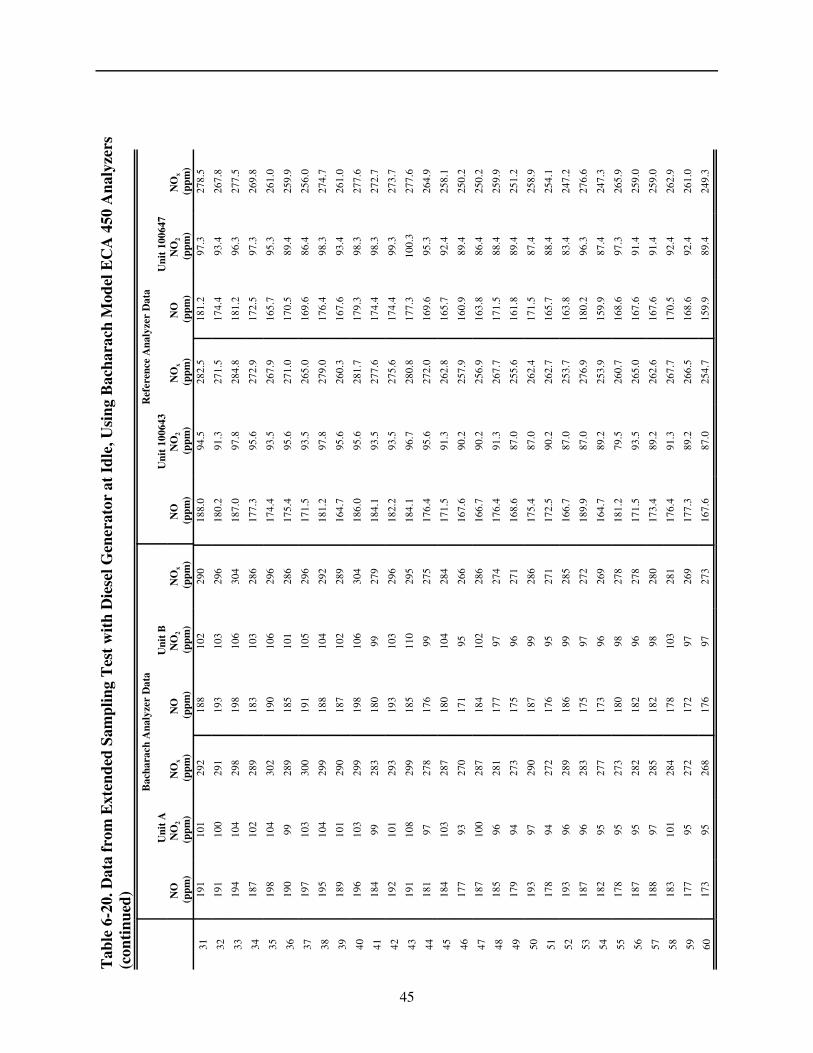
The last operation in the combustion source testing involved continuous sampling of the dieselengine emissions for a full hour with no intervals of room air sampling. Data were recorded forboth reference and vendor analyzers at 1-minute intervals throughout that hour of measurement.This extended sampling was conducted only after nine sequential sets of readings had beenobtained from all the combustion sources by the procedure described above. Results from thisextended sampling were used to determine the measurement stability of the ECA 450 analyzer.

15

Chapter 4Quality Assurance/Quality Control

Quality control (QC) procedures were performed in accordance with the quality managementplan (QMP) for the AMS Center(7) and the test/QA plan(1) for this verification test.

4.1 Data Review and Validation

Test data were reviewed and approved according to the AMS Center QMP, the test/QA plan, andBattelle’s one-over-one approval policy. The Verification Testing Leader reviewed the raw dataand data sheets that were generated each day. Laboratory record notebooks were also signed anddated by testing staff and reviewed by the Verification Testing Leader.

Other data review focused upon the compliance of the reference analyzer data with the qualityrequirements of Method 7E. The purpose of validating reference data was to ensure usability forthe purposes of comparison with the demonstration technologies. The results of the review of thereference analyzer data quality are shown in Table 4-1. The data generated by the referenceanalyzers were used as a baseline to assess the performance of the technologies for NO/NO2

analysis.

4.2 Deviations from the Test/QA Plan

During the physical set up of the verification test, deviations from the test/QA plan were made tobetter accommodate differences in vendor equipment, and other changes or improvements. Anydeviation required the approval signature of Battelle’s Verification Testing Leader and CenterManager. A planned deviation form was used for documentation and approval of the followingchanges:

1. The order of testing was changed in the pressure sensitivity test to require fewer plumbingchanges in conducting the test.

2. The order of the ambient temperature test was changed to maximize the detection of anytemperature effect.

3. The concentrations used in the mixture of SO2 and NO for the interference test werechanged slightly.

4. For better accuracy, the oxygen sensor used during combustion source tests was checked bycomparison to an independent paramagnetic O2 sensor, rather than to a wet chemicalmeasurement.

5. Single points (rather than triplicate points) were run at each calibration level in calibratingthe reference analyzers, in accord with Method 7E.

16

Table 4-1. Results of QC Procedures for Reference Analyzers for Testing ofBacharach Model ECA 450 Analyzers

NO2 conversionefficiency (Unit 100643)

91.8%

NO2 conversionefficiency (Unit 100647)

99.3%

Calibration of referencemethod using four pointsat 0, 30, 60, 100% forNO

Meets criteria (r2 = 0.9999)

Calibration of referencemethod using four pointsat 0, 30, 60, 100% forNO2

Meets criteria (r2 = 0.9999)

Calibrations (100 ppm range)

Meet ± 2% requirement (relativeto span) Unit 100643 Unit 100647

NO NO

Error, % ofSpan

at % of Scale

Error, % ofSpan

at % of Scale

0.5 30 0.5 30

0.8 60 0.5 60

NO2 NO2

Error, % ofSpan

at % of Scale

Error, % ofSpan

at % of Scale

0.4 30 0.3 30

0.7 60 0.8 60

Zero drift Meets ± 3% requirement (relativeto span) on all combustionsources

Span drift Meets ± 3% requirement (relativeto span) on all combustionsources

Interference check < ± 2% (no interference responseobserved)

6. A short, unheated sample inlet was used with the reference analyzers, based on pre-test trialruns, on Battelle’s previous experience in sampling the combustion sources used in this test,and on other similar sources.

7. No performance evaluation audit was conducted on the natural gas flow rate measurementused with the gas water heater. This measurement was made with a newly calibrated dry gasmeter.

17

4.3 Calibration of Laboratory Equipment

Equipment used in the verification test required calibration before use, or verification of themanufacturer’s calibrations. Some auxiliary devices were obtained with calibration fromBattelle’s Instrument Laboratory. Equipment types and calibration dates are listed in Table 4-2.For key equipment items, the calibrations listed include performance evaluation audits (seeSection 4.5.2). Documentation of calibration of the following equipment was maintained in thetest file.

Table 4-2. Equipment Type and Calibration Date

Equipment Type UseCalibration/PE

Date

Gas Dilution System Environics Model 4040 (Serial Number 2469)

Lab tests 3/9/00; 5/9/00

Gas Dilution System Environics Model 2020 (Serial Number 2108)

Source tests 3/20/00; 5/9/00

Fluke Digital Thermometer(LN-570068)

Ambient temperaturetest

10/15/99; 5/26/00

Servomex 570A Analyzer (X-44058)

Flue gas O2 11/22/99; 5/18/00

Dwyer Magnahelic Pressure Gauge Pressure sensitivitytest

4/7/00

Doric Trendicator 410A Thermocouple Temperature Sensor (Serial Number 331513)

Flue gas temperature 8/5/99; 5/26/00

American Meter DTM 115 Dry Gas Meter(Serial Number 89P124205)

Gas flowmeasurement

4/17/00

4.4 Standard Certifications

Standard or certified gases were used in all verification tests, and certifications or analytical datawere kept on file to document the traceability of the following standards:

� EPA Protocol Gas Nitrogen Dioxide� EPA Protocol Gas Nitric Oxide� Certified Master Class Calibration Standard Sulfur Dioxide� Certified Master Class Calibration Standard Carbon Dioxide� Certified Master Class Calibration Standard Ammonia� Certified Master Class Calibration Standard Carbon Monoxide� Nitrogen Acid Rain CEM Zero

18

� Acid Rain CEM Zero Air� Battelle-Prepared Organics Mixture.

All other QC documentation and raw data for the verification test are located in the test file atBattelle, to be retained for 7 years and made available for review if requested.

4.5 Performance System Audits

Three internal performance system audits were conducted during verification testing. A technicalsystems audit was conducted to assess the physical setup of the test, a performance evaluationaudit was conducted to evaluate the accuracy of the measurement system, and an audit of dataquality was conducted on 10% of all data generated during the verification test. A summary ofthe results of these audits is provided below.

4.5.1 Technical Systems Audit

A technical systems audit (TSA) was conducted on April 18, 2000, (laboratory testing) andMay 17 and 18, 2000, (source testing) for the NO/NO2 verification tests conducted in early 2000.The TSA was performed by the Battelle’s Quality Manager as specified in the AMS CenterQuality Management Plan (QMP). The TSA ensures that the verification tests are conductedaccording to the test/QA plan(1) and all activities associated with the tests are in compliance withthe AMS Center QMP(7). All findings noted during the TSA on the above dates were documentedand submitted to the Verification Testing Leader for correction. The corrections were docu-mented by the Verification Testing Leader and reviewed by Battelle’s Quality Manager andCenter Manager. None of the findings adversely affected the quality or outcome of thisverification test and all were resolved to the satisfaction of the Battelle Quality Manager. Therecords concerning the TSA are permanently stored with the Battelle Quality Manager.

4.5.2 Performance Evaluation Audit

The performance evaluation audit was a quantitative audit in which measurement standards wereindependently obtained and compared with those used in the verification test to evaluate theaccuracy of the measurement system. That assessment was conducted by Battelle testing staff onMay 23 and 26, 2000, and the results were reviewed by independent QA personnel.

The most important performance evaluation (PE) audit was of the standards used for thereference measurements in source testing. The PE standards were NO and NO2 calibration gasesindependent of the test calibration standards that contained certified concentrations of NO andNO2. Accuracy of the reference analyzers was determined by comparing the measured NO/NO2

concentrations using the verification test standards with those obtained using the certified PEstandards. Percent difference was used to quantify the accuracy of the results. The PE sample forNO was an EPA Protocol Gas having a concentration (3,988 ppm) nearly the same as the NOstandard used in verification testing, but purchased from a different commercial supplier(Matheson Gas Products). The PE standard for NO2 was a similar commercial standard of463 ppm NO2 in air, also from Matheson. Table 4-3 summarizes the NO/NO2 standard method

19

performance evaluation results. Included in this table are the performance acceptance ranges andthe certified gas concentration values. The acceptance ranges are guidelines established by theprovider of the PE materials to gauge acceptable analytical results.

Table 4-3 shows that the PE audit confirmed the concentration of the Scott 3,925 ppm NO teststandard almost exactly: the apparent test standard concentration was within 0.2% of the teststandard’s nominal value. On the other hand, the PE audit results for the Scott 511.5 ppm NO2

standard were not as close. The comparison to the Matheson PE standard indicated that the511.5 ppm NO2 Scott standard was only about 480 ppm, a difference of about 7% from itsnominal value. This result suggests an error in the Scott test standard for NO2. However, aseparate line of evidence indicates that the Matheson PE standard is likely in error. Specifically,conversion efficiency checks on the reference analyzers (performed by comparing their responsesto the Scott NO and NO2 standards) consistently showed the efficiency of the converter in 42-CUnit 100647 to be very close to 100%. This finding could not occur if the concentration of theNO2 standard were low. That is, a conversion efficiency of 100% indicates agreement betweenthe NO standard and the NO2 standard; and, as shown in Table 4-3, the NO standard is confirmedby the PE comparison. Thus, the likelihood is that the Matheson PE standard was in fact some-what higher in concentration than its nominal 463 ppm value.

PE audits were also done on the O2 sensor used for flue gas measurements, and on thetemperature indicators used for ambient and flue gas measurements. The PE standard for O2

was an independent paramagnetic sensor, and for temperature was a certified mercury-in-glassthermometer. The O2 comparison was conducted during sampling of diesel exhaust; the tempera-ture comparisons were conducted at room temperature. The results of those audits are shown inTable 4-4, and indicate close agreement of the test equipment with the PE standards.

4.5.3 Audit of Data Quality

The audit of data quality is a qualitative and quantitative audit in which data and data handlingare reviewed and data quality and data usability are assessed. Audits of data quality are used tovalidate data at the frequency of 10% and are documented in the data audit report. The goal of anaudit of data quality is to determine the usability of test results for reporting technologyperformance, as defined during the design process. Validated data are reported in the ETVverification reports and ETV verification statement along with any limitations on the data andrecommendations for limitations on data usability.

The Battelle Quality manager audited 10% of the raw data. Test data sheets and laboratory recordbooks were reviewed, and statistical calculations and other algorithms were verified. Calculationsthat were used to assess the four-point calibration of the reference method were also verified tobe correct. In addition, data presented in the verification report and statement are audited toensure accurate transcription.

20

Table 4-3. Performance Evaluation Results on NO/NO2 Standards

ReferenceAnalyzer/Standard

Reading on Diluted Standard

ApparentConcentrationa

PercentDifferenceb

AcceptanceLimits

Unit 100643NO in N2

(ppm)Test Std 3,925 98.8 ppm 3,917 ppm 0.2% ±2%PE Std 3,988 100.6 ppm

Unit 100647NO in N2

(ppm)Test Std 3,925 99.6 ppm 3,917 ppm 0.2% ±2%PE Std 3,988 101.4 ppm

Unit 100643NO2 in Air

(ppm)Test Std 511.5 44.2 ppm 482 ppm 5.8% ±5%PE Std 463 42.5 ppm

Unit 100647NO2 in Air

(ppm)Test Std 511.5 49.6 ppmPE Std 463 48.8 ppm 471 ppm 7.9% ±5%a Concentration of Test Standard indicated by comparison to the Performance Evaluation Standard; i.e., Apparent

Concentration = (Test Std. Reading/PE Std. Reading) × PE Std. Conc.; e.g., Apparent Concentration = 98.8/100.6× 3,988 ppm = 3,917 ppm.

b Percent difference of Apparent Concentration relative to Test Standard concentration; e.g., percent difference =

3 ,9 25 p pm - 3 ,91 7 pp m

3,9 25 p pm X 10 0 0 .2% .=

Table 4-4. Performance Evaluation Results in O2 and Temperature Measuring Equipment

Analyzer Reading Difference Acceptance Limits

Servomex 570A O2 18.9% O2 0% O2 –PE Standarda 18.9% O2

Fluke Digital Thermometer 22.1�C 0.1�C 2% absolute TPE Standardb 22�C

Doric 410A Temp. Sensor 24.8�C 0.2�C 2% absolute TPE Standardb 25.0�C 0.2�C

a Independent paramagnetic O2 analyzer.b Certified mercury-in-glass thermometer.

21

Yc � h(c) � errorc

�2c �� kc �

weight � wc �1

�2c

Chapter 5Statistical Methods


The analyzer performance characteristics were quantified on the basis of statistical comparisonsof the test data. This process began by converting the spreadsheet files that resulted from the dataacquisition process into data files suitable for evaluation with Statistical Analysis System (SAS)software. The following statistical procedures were used to make those comparisons.

5.1.1 Linearity

Linearity was assessed by linear regression with the calibration concentration as the independentvariable and the analyzer response as the dependent variable. Separate assessments were carriedout for each EAC 450 analyzer. The calibration model used was

where Yc is the analyzer’s response to a challenge concentration c, h(c) is a linear calibrationcurve, and the error term was assumed to be normally distributed. (If the variability is notconstant throughout the range of concentrations then weighting in the linear regression isappropriate. It is often the case that the variability increases as the true concentration increases.)The variability (�c) of the measured concentration values (c) was modeled by the followingrelationship,

where �, k, and � are constants to be estimated from the data. After determining the relationshipbetween the mean and variability, appropriate weighting was determined as the reciprocal of thevariance.

22

c � h 1(Yc ) �

Yc � �o

�1

14�

6

i1(Yci

� �o � �1ci)2nci

wci

LOD �

(�o � 3�o ) � �o

�1

�

3�o

�1

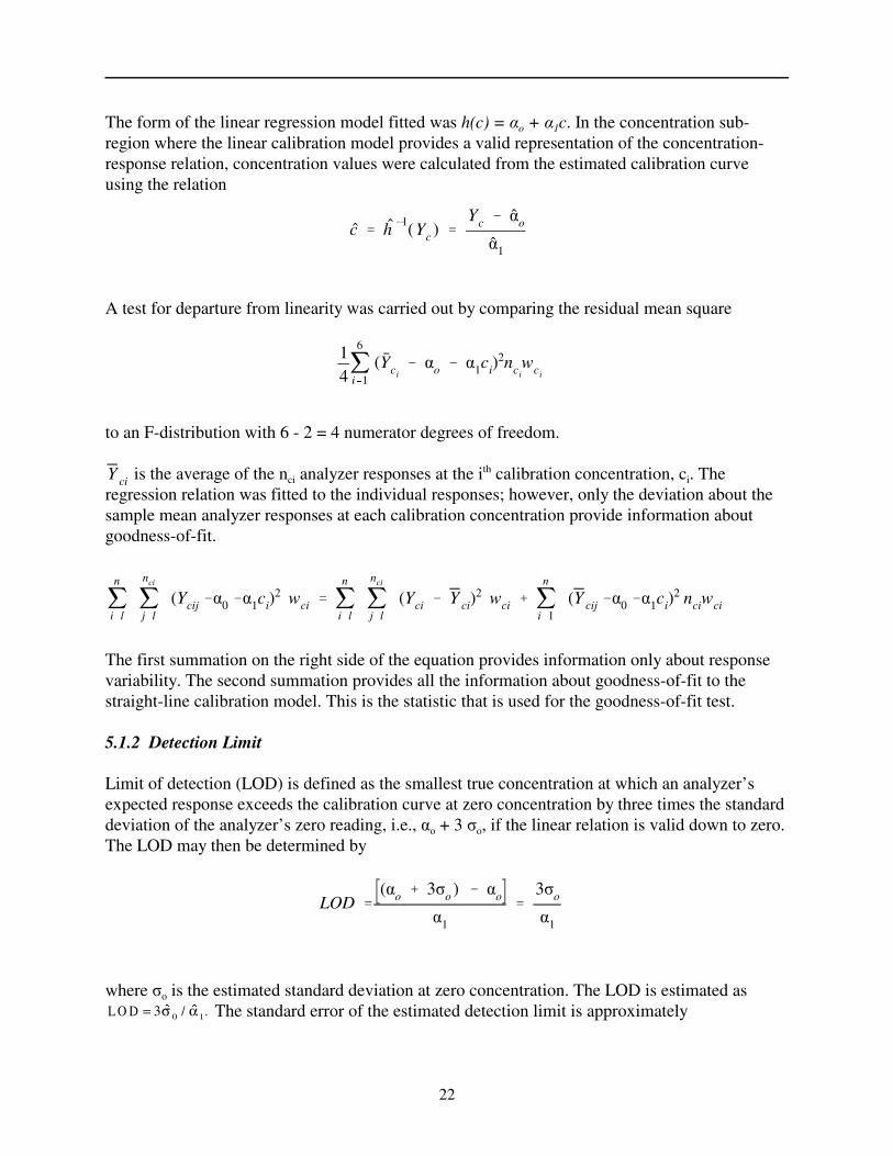
The form of the linear regression model fitted was h(c) = �o + �1c. In the concentration sub-region where the linear calibration model provides a valid representation of the concentration-response relation, concentration values were calculated from the estimated calibration curveusing the relation

A test for departure from linearity was carried out by comparing the residual mean square

to an F-distribution with 6 - 2 = 4 numerator degrees of freedom.

is the average of the nci analyzer responses at the ith calibration concentration, ci. TheY ciregression relation was fitted to the individual responses; however, only the deviation about thesample mean analyzer responses at each calibration concentration provide information aboutgoodness-of-fit.

�n

il�

nci

jl(Ycij ��0 ��1ci)

2 wci � �n

il�

nci

jl(Yci � Y ci)

2 wci � �n

i1(Y cij ��0 ��1ci)

2 nciwci

The first summation on the right side of the equation provides information only about responsevariability. The second summation provides all the information about goodness-of-fit to thestraight-line calibration model. This is the statistic that is used for the goodness-of-fit test.


Limit of detection (LOD) is defined as the smallest true concentration at which an analyzer’sexpected response exceeds the calibration curve at zero concentration by three times the standarddeviation of the analyzer’s zero reading, i.e., �o + 3 �o, if the linear relation is valid down to zero.The LOD may then be determined by

where �o is the estimated standard deviation at zero concentration. The LOD is estimated as The standard error of the estimated detection limit is approximatelyL O D = 3 0 1

� / � .σ α

23

SE (LOD)ˆ� LODˆ 1

2(n�1)�

SE (a1)

a1

2

Note that the validity of the detection limit estimate and its standard error depends on the validityof the assumption that the fitted linear calibration model accurately represents the response downto zero concentration.

5.1.3 Response Time

The response time of the ECA 450 analyzers to a step change in analyte concentration wascalculated by determining the total change in response due to the step change in concentration,and then determining the point in time when 95% of that change was achieved. Using data takenevery 10 seconds, the following calculation was carried out:

Total Response = Rc - Rz

where Rc is the final response of the analyzer to the calibration gas and Rz is the final response ofthe analyzer to the zero gas. The analyzer response that indicates the response time then is:

Response95% = 0.95(Total Response) + Rz.

The point in time at which this response occurs was determined by inspecting the response/timedata, linearly interpolating between two observed time points, as necessary. The response timewas calculated as:

RT = Time95% - TimeI,

where Time95% is the time at which ResponseRT occurred and TimeI is the time at which the spangas was substituted for the zero gas. Since only one measurement was made, the precision of theresponse time was not determined.


The effect of interrupted sampling is the arithmetic difference between the zero data and betweenthe span data obtained before and after the test. Differences are stated as ppm. No estimate wasmade of the precision of the observed differences.

5.1.5 Interferences

Interference is reported as both the absolute response (in ppm) to an interferant level, and as thesensitivity of the analyzer to the interferant species, relative to its sensitivity to NO or NO2. Therelative sensitivity is defined as the ratio of the observed NO/NO2/NOx response of the analyzerto the actual concentration of the interferant. For example, an analyzer that measures NO is

24

challenged with 500 ppm of CO, resulting in an absolute difference in reading of 1 ppm (as NO).The relative sensitivity of the analyzer is thus 1 ppm/500 ppm = 0.2%. The precision of theinterference results was not estimated from the data obtained, since only one measurement wasmade for each interferant.


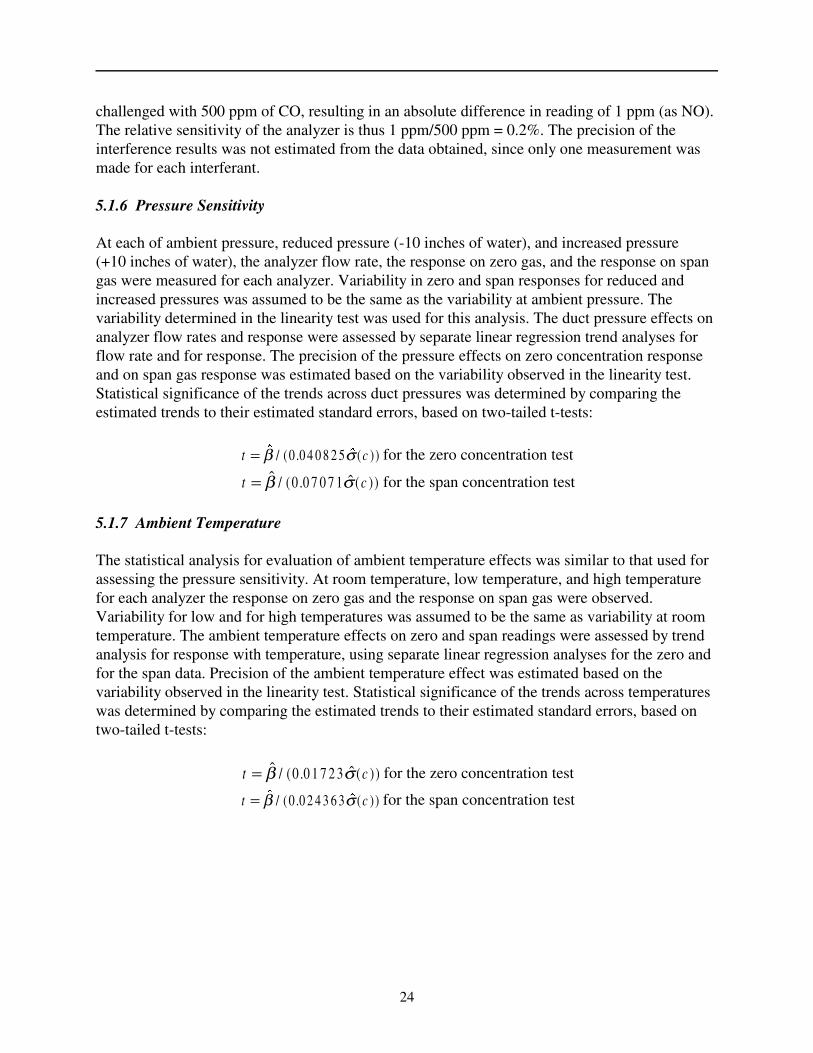
At each of ambient pressure, reduced pressure (-10 inches of water), and increased pressure(+10 inches of water), the analyzer flow rate, the response on zero gas, and the response on spangas were measured for each analyzer. Variability in zero and span responses for reduced andincreased pressures was assumed to be the same as the variability at ambient pressure. Thevariability determined in the linearity test was used for this analysis. The duct pressure effects onanalyzer flow rates and response were assessed by separate linear regression trend analyses forflow rate and for response. The precision of the pressure effects on zero concentration responseand on span gas response was estimated based on the variability observed in the linearity test.Statistical significance of the trends across duct pressures was determined by comparing theestimated trends to their estimated standard errors, based on two-tailed t-tests:

for the zero concentration testt c= � / ( . � ( ) )β σ0 0 4 0 8 2 5

for the span concentration testt c= � / ( . � ( ) )β σ0 0 7 0 7 1


The statistical analysis for evaluation of ambient temperature effects was similar to that used forassessing the pressure sensitivity. At room temperature, low temperature, and high temperaturefor each analyzer the response on zero gas and the response on span gas were observed.Variability for low and for high temperatures was assumed to be the same as variability at roomtemperature. The ambient temperature effects on zero and span readings were assessed by trendanalysis for response with temperature, using separate linear regression analyses for the zero andfor the span data. Precision of the ambient temperature effect was estimated based on thevariability observed in the linearity test. Statistical significance of the trends across temperatureswas determined by comparing the estimated trends to their estimated standard errors, based ontwo-tailed t-tests:

for the zero concentration testt c= � / ( . � ( ) )β σ0 0 1 7 2 3

for the span concentration testt c= � / ( . � ( ) )β σ0 0 2 4 3 6 3

25

RA �

� d� � t .n1

Sd

nx

× 100%

SE �Sd

n x0.3634 � t a

n12 1

2 n�1× 100%


5.2.1 Accuracy

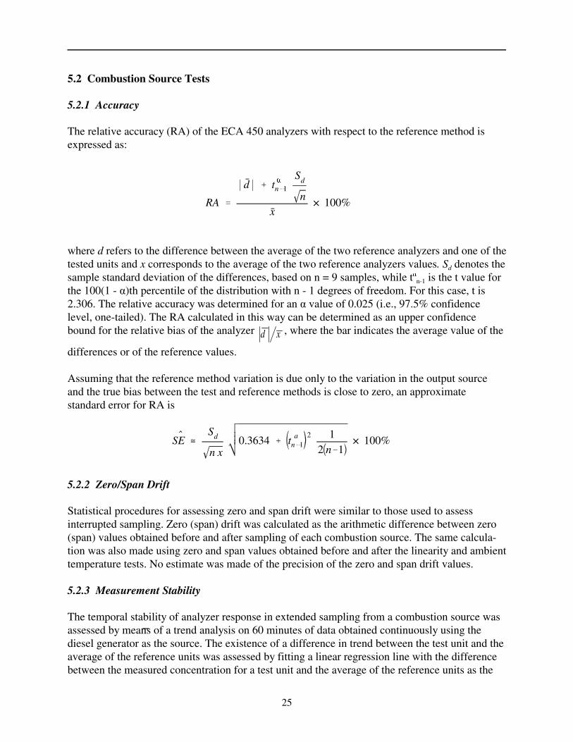
The relative accuracy (RA) of the ECA 450 analyzers with respect to the reference method isexpressed as:

where d refers to the difference between the average of the two reference analyzers and one of thetested units and x corresponds to the average of the two reference analyzers values. Sd denotes thesample standard deviation of the differences, based on n = 9 samples, while t.n-1 is the t value forthe 100(1 - �)th percentile of the distribution with n - 1 degrees of freedom. For this case, t is2.306. The relative accuracy was determined for an � value of 0.025 (i.e., 97.5% confidencelevel, one-tailed). The RA calculated in this way can be determined as an upper confidencebound for the relative bias of the analyzer , where the bar indicates the average value of thed x

differences or of the reference values.

Assuming that the reference method variation is due only to the variation in the output sourceand the true bias between the test and reference methods is close to zero, an approximatestandard error for RA is

5.2.2 Zero/Span Drift

Statistical procedures for assessing zero and span drift were similar to those used to assessinterrupted sampling. Zero (span) drift was calculated as the arithmetic difference between zero(span) values obtained before and after sampling of each combustion source. The same calcula-tion was also made using zero and span values obtained before and after the linearity and ambienttemperature tests. No estimate was made of the precision of the zero and span drift values.

5.2.3 Measurement Stability

The temporal stability of analyzer response in extended sampling from a combustion source wasassessed by means of a trend analysis on 60 minutes of data obtained continuously using thediesel generator as the source. The existence of a difference in trend between the test unit and theaverage of the reference units was assessed by fitting a linear regression line with the differencebetween the measured concentration for a test unit and the average of the reference units as the

26

dependent variable, and time as the independent variable. Subtracting the average reference unitvalues adjusts for variation in the source output. The slope and the standard error of the slope arereported. The null hypothesis that the slope of the trend line on the difference is zero was testedusing a one-sample two-tailed t-test with n - 2 = 58 degrees of freedom.

5.2.4 Inter-Unit Repeatability

The purpose of this comparison was to determine if any significant differences in performanceexist between two identical analyzers operating side by side. In tests in which analyzer per-formance was verified by comparison with data from the reference method, the two identicalunits of each type of analyzer were compared to one another using matched pairs t-testcomparisons. In tests in which no reference method data were obtained (e.g., linearity test), thetwo ECA 450 analyzer units were compared using statistical tests of difference. For example, theslopes of the calibration lines determined in the linearity test, and the detection limits determinedfrom those test data, were compared. Inter-unit repeatability was assessed for the linearity,detection limit, accuracy, and measurement stability tests.

For the linearity test, the intercepts and slopes of the two units were compared to one another bytwo-sample t-tests using the pooled standard error, with combined degrees of freedom the sum ofthe individual degrees of freedom.

For the detection limit test, the detection limits of the two units were compared to one another bytwo-sample t-tests using the pooled standard error with 10 degrees of freedom (the sum of theindividual degrees of freedom).

For the relative accuracy test, repeatability was assessed with a matched-pairs two-tailed t-testwith n - 1 = 8 degrees of freedom.

For the measurement stability test, the existence of differences in trends between the two unitswas assessed by fitting a linear regression to the paired differences between the units. The nullhypothesis that the slope of the trend line on the paired differences is zero was tested using amatched-pairs t-test with n - 2 = 58 degrees of freedom.

5.2.5 Data Completeness

Data completeness was calculated as the percentage of possible data recovered from an analyzerin a test; the ratio of the actual to the possible number of data points, converted to a percentage,i.e.,

Data Completeness = (Na)/(Np) x 100%,

where Na is the number of actual and Np the number of planned data points.

27

Chapter 6Test Results


6.1.1 Linearity

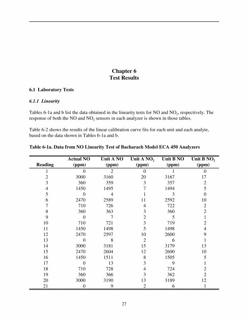
Tables 6-1a and b list the data obtained in the linearity tests for NO and NO2, respectively. Theresponse of both the NO and NO2 sensors in each analyzer is shown in those tables.

Table 6-2 shows the results of the linear calibration curve fits for each unit and each analyte,based on the data shown in Tables 6-1a and b.

Table 6-1a. Data from NO Linearity Test of Bacharach Model ECA 450 Analyzers

ReadingActual NO

(ppm)Unit A NO

(ppm)Unit A NO2

(ppm)Unit B NO

(ppm)Unit B NO2

(ppm)1 0 2 0 1 02 3000 3160 20 3167 173 360 359 3 357 24 1450 1495 7 1494 55 0 4 1 3 06 2470 2589 11 2592 107 710 726 4 722 28 360 363 3 360 29 0 7 2 5 1

10 710 721 3 719 211 1450 1498 5 1498 412 2470 2597 10 2600 913 0 8 2 6 114 3000 3181 15 3179 1315 2470 2604 12 2600 1016 1450 1511 8 1505 517 0 13 3 9 118 710 728 4 724 219 360 366 3 362 220 3000 3190 13 3189 1221 0 9 2 6 1

28

Table 6-1b. Data from NO2 Linearity Test of Bacharach Model ECA 450 Analyzers

NumberActual NO2

(ppm)Unit A NO

(ppm)Unit A NO2

(ppm)Unit B NO

(ppm)Unit B NO2

(ppm)1 0 0 0 0 02 450 4 453 4 4533 45 0 49 0 504 210 1 213 1 2145 0 0 1 0 26 350 3 354 3 3547 100 0 103 0 1048 45 0 47 0 489 0 0 1 0 110 100 0 102 0 10311 210 1 213 1 21412 350 3 358 0 35913 0 0 2 0 314 450 4 457 4 45615 350 3 358 0 36016 210 2 216 2 21917 0 0 3 0 418 100 0 103 0 10519 45 0 47 0 4820 450 5 457 5 45821 0 0 2 0 3

Table 6-2. Statistical Results for Test of Linearity

Linear Regression

Unit A Unit B

NO NO2 NO NO2

Intercept (ppm) (Std Err) -0.913 (3.680) 1.669 (0.319) -4.610 (3.950) 3.860 (1.274)Slope (Std Err) 1.048 (0.004) 1.011 (0.002) 1.049 (0.004) 1.007 (0.004)r2 0.9997 0.9999 0.9997 0.9998

The results in Table 6-2 show that the NO2 response of the ECA 450 analyzers was linear overthe entire range tested of up to 450 ppm. The NO2 slopes are both approximately 1.01, and the r2

values are 0.9998 or higher.

The NO linearity results in Table 6-2 show that, over the tested range of up to 3,000 ppm NO, theECA 450 analyzers gave negative intercept values and slopes of about 1.05, significantlyexceeding the upper limit of 1.02 generally expected of these analyzers.(8) Inspection of the NOlinearity data, plotted in Figure 6-1, shows that the NO response of the ECA 450 analyzers islinear at lower concentrations, but exhibits an upward curvature at higher concentrations,

29

NO Linearity Tests of Bacharach ECA 450

0

500

1000

1500

2000

2500

3000

3500

0.0 500.0 1000.0 1500.0 2000.0 2500.0 3000.0 3500.0

Actual NO, ppm

EC

A 4

50 R

esp

on

se, p

pm

NO

Unit A

Unit B

1 to 1

Figure 6-1. Plot of NO Linearity Data

resulting in the overall regression results shown in Table 6-2. For example, the regression slopesfor the two ECA 450 units are 1.007 and 1.009 when the lowest 12 calibration points inTable 6-1a (i.e., up to 710 ppm) are included, but increase to about 1.03 when the lowest 15 datapoints (i.e., up to 1,450 ppm) are included. These results suggest that the linear range of NOresponse for the ECA 450 analyzers is about 1,000 ppm, with increasing upward curvature ofresponse above that level.

The data in Tables 6-1a and 6-1b also indicate the extent of cross-sensitivity of the BacharachNO and NO2 sensors. Regression of the ECA 450 NO2 responses in the NO linearity test(Table 6-1a) gives the regression results:

Unit A NO2 = 0.0044 ×(NO, ppm) + 1.17 ppm, with r2 = 0.904, andUnit B NO2 = 0.0042 ×(NO, ppm) + 0.05 ppm, with r2 = 0.926.

These results indicate a very slight response of the Bacharach NO2 sensors to NO, amounting toabout 0.4% of the NO level present.

30

Similarly, regression of the ECA 450 NO responses in the NO2 linearity test (Table 6-1b) givesthe regression results:

Unit A NO = 0.0097 ×(NO2, ppm) - 0.36 ppm, with r2 = 0.932, andUnit B NO = 0.0078 ×(NO2, ppm) - 0.33 ppm, with r2 = 0.651.

These results also indicate a very small response of the Bacharach NO sensors to NO2,amounting to less than 1% of the NO2 level present.


Table 6-3 shows the estimated detection limits for each test unit and each analyte, determinedfrom the data obtained in the linearity test. These detection limits apply to the calibrationsconducted over a 0 to 3,000 ppm range for NO (Table 6-1a) and a 0 to 450 ppm range for NO2

(Table 6-1b).

Table 6-3. Estimated Detection Limits for Bacharach Model ECA 450 Analyzersa

Unit A Unit B

NO NO2 NO NO2

Estimated Detection Limit (ppm) 11.1 3.1 7.9 4.4

(Standard Error) (ppm) (3.5) (1.0) (2.5) (1.4)a Results are based on calibrations over 0-3,000 ppm range for NO and 0-450 ppm range for NO2.

Table 6-3 displays the estimated detection limits, and their standard errors for NO and NO2,separately for each ECA 450 analyzer. NO detection limits of 8 to 11 ppm, and NO2 detectionlimits of 3 to 4 ppm, are indicated. It must be stressed that these detection limits are based on thezero gas responses interspersed with sampling of high levels of NO and NO2 in the linearity tests.As shown in Tables 6-1a and 6-1b, the zero gas responses tended to increase steadily throughoutthe linearity tests as a result of the exposures to high concentrations. Substantially lower detec-tion limits are suggested by the results of the source testing (see Section 6.2), which show that, inthe absence of this memory effect (due to high concentration exposures), detection limits for bothNO and NO2 appear to be comparable to the 1 ppm resolution of the analyzer.

6.1.3 Response Time

Table 6-4 lists the data obtained in the response time test of the ECA 450 analyzers. Table 6-5shows the response times of the analyzers to a step change in analyte concentration, based on thedata shown in Table 6-4. Table 6-5 shows that the response times of the two ECA 450 analyzerswere consistent, i.e., 28 to 29 seconds for NO, and 54 to 57 seconds for NO2. These responsetimes are more than sufficient for source emission measurements and are well within the4-minute response criteria required of portable NO/NOx analyzers.(8)

31

Table 6-4. Response Time Data for Bacharach Model ECA 450 Analyzers

Time (sec)Unit A NO

(ppm)Unit A NO2

(ppm)Unit B NO

(ppm)Unit B NO2

(ppm) 0 4 1 2 210 601 55 709 2820 2294 225 2267 19930 2537 288 2546 27340 2600 319 2597 31150 2614 333 2610 32960 2620 342 2614 34070 2624 346 2617 34480 2626 349 2619 34790 2628 350 2621 349

100 2629 351 2622 351110 2630 352 2623 352120 2632 353 2624 353130 2633 354 2625 354140 2633 354 2626 354150 2634 354 2627 354160 2635 2627170 2636 2628

Table 6-5. Response Time Results for Bacharach Model ECA 450 Analyzers

Unit A Unit BNO NO2 NO NO2

Response Time (sec)a 29 54 28 57

a The analyzer’s responses were recorded at 10-second intervals; therefore the point in time when the 95%response was achieved was determined by interpolating between recorded times to the nearest second.


Table 6-6 shows the zero and span data resulting from the interrupted sampling test, andTable 6-7 shows the differences (pre- minus post-) of the zero and span values. Span con-centrations of 3,000 ppm NO and 450 ppm NO2 were used for this test.

The change in zero levels observed as a result of the shutdown period are larger for NO than forNO2. This difference, and the changes in zero values themselves, probably results from theexposure to elevated NO and NO2 levels in the linearity tests that immediately preceded theshutdown. That is, the small changes in zero readings are probably the result of the analyzersreturning to baseline readings after the linearity tests.

32

The ECA 450 analyzers showed essentially no change in the NO2 span response as a result of theshutdown (Table 6-7). The changes observed in the NO span response are much larger (168 and208 ppm), and amount to 5.6 and 6.9% of the 3,000 ppm NO span value.

Table 6-6. Data from Interrupted Sampling Test with Bacharach Model ECA 450Analyzers

Unit A NO Unit A NO2 Unit B NO Unit B NO2

Pre-Shutdown Date: 04/17/2000 Time: 15:15Pre-Shutdown Zero (ppm): 6 2 3 1Pre-Shutdown Span (ppm): 3325 457 3264 455

Post-Shutdown Date: 04/18/2000 Time: 8:00Post-Shutdown Zero (ppm): 0 0 0 0Post-Shutdown Span (ppm): 3117 458 3096 457

Table 6-7. Pre- to Post-Test Differences as a Result of Interruption of Operation ofBacharach Model ECA 450 Analyzers

Pre-Shutdown—Post-Shutdown

Unit A Unit B

NO NO2 NO NO2

Zero Difference (ppm) 6 2 3 1

Span Difference (ppm) 208 -1 168 -2

6.1.5 Interferences

Table 6-8 lists the data obtained in the interference tests. Table 6-9 summarizes the sensitivity ofthe analyzers to interferant species, based on the data from Table 6-8. The results in Table 6-8use the average of the zero readings before and after the interferant exposure to calculate theextent of the interference.

Table 6-9 indicates that no significant interference effects from CO, CO2, NH3, HCs, and SO2

were found. However, the response to 393 ppm NO was considerably reduced by the presence of451 ppm SO2, indicating a relative sensitivity to SO2 of about -9 to -10%. It should be noted thatthe vendor was not able to reproduce this effect in his own laboratories, using up to 500 ppmeach of NO and SO2, and has observed no significant interference from SO2 in the presence ofNO with the ECA 450 analyzer.

33

Table 6-8. Data from Interference Tests on Bacharach Model ECA 450 Analyzers

Interferant, Conc.(ppm)

Response (ppm equivalent)Unit A NO2 Unit B NO Unit B NO2

InterferantGas Unit A NO

Zero 0 4 0 3CO 496 0 3 0 2Zero 0 2 0 2CO2 5.03% 0 3 0 3Zero 0 3 0 3NH3 494 0 1 0 1Zero 0 0 0 0HCs 605 0 1 0 0Zero 0 0 0 0SO2 501 0 0 0 0Zero 0 0 0 0SO2 + NO 451 + 393 354 1 347 1

Table 6-9. Results of Interference Tests of Bacharach Model ECA 450 Analyzers

Interferant

Unit A Response ppm(relative sensitivity, %)

Unit B Response ppm(relative sensitivity, %)

NO NO2 NO NO2

CO (496 ppm) 0 0% 0 0.1%CO2 (5.03%) 0 <0.01% 0 <0.01%NH3 (494 ppm) 0 -0.2% 0 -0.2%HCs (605 ppm) 0 <0.2% 0 0SO2 (501 ppm) 0 0 0 0

SO2 (451 ppm) + NO (393 ppm)

-8.6% 0.2% -10.2% 0.2%


Table 6-10 lists the data obtained in the pressure sensitivity test. Table 6-11 summarizes thefindings from those data in terms of the ppm differences in zero and span readings at the differentduct gas pressures, and the ccm differences in analyzer flow rates at the different duct gaspressures.

Tables 6-10 and 6-11 show that only very small changes in ECA 450 zero readings resulted fromthe changes in duct pressure, for both NO and NO2. The changes observed do not indicate anystatistically significant effect of pressure on zero readings. In contrast, an effect of pressure was

34

seen on span responses for both NO and NO2 with both ECA 450 analyzers. The effect wasconsistent, in that lower pressure produced lower response, for both species on both ECA 450analyzers. The total difference in span responses between +8.5 and -8.5 in. H2O amounted toabout 3.7 to 7.5% of the 3,000 ppm NO span value, and to about 8 to 14% of the 450 ppm NO2

span value.

Tables 6-10 and 6-11 also show a substantial effect of pressure on the sample flow rates of theECA 450 analyzers. The reduced pressure condition reduced the sample flow rates by only about6 to 15% relative to the flows at ambient pressure. However, under the positive pressurecondition, the flow rates of both units were more than doubled.

Table 6-10. Data from Pressure Sensitivity Test for Bacharach Model ECA 450 Analyzers

Pressure Unit A NO Unit A NO2 Unit B NO Unit B NO2

Ambient Flow rate (ccm) 804 804 774 774Zero (ppm) 0 0 0 0NO span (ppm) 3209 11 3163 10Zero (ppm) 0 1 0 1NO2 span (ppm) 0 460 0 467Zero (ppm) 0 2 0 1

+8.5 in. H2O Flow rate (ccm) 1766 1766 1696 1696Zero (ppm) 0 1 0 0NO span (ppm) 3318 11 3224 10Zero (ppm) 0 2 0 1NO2 span (ppm) 0 475 0 500Zero (ppm) 0 2 0 2

-8.5 in. H2O Flow rate (ccm) 691 691 730 730Zero (ppm) 0 2 0 1NO span (ppm) 3093 11 3112 11Zero (ppm) 0 3 0 1NO2 span (ppm) 0 439 0 438Zero (ppm) 0 3 0 4

35

Table 6-11. Pressure Sensitivity Results for Bacharach Model ECA 450 Analyzers

Unit A Unit BNO NO2 NO NO2

Zero High–Ambient (ppm diff*) 0 0.667 0 0.333Low–Ambient (ppm diff) 0 1.667 0 1.333Significant Pressure Effect N N N N

Span High–Ambient (ppm diff) 109 15 61 33Low–Ambient (ppm diff) -116 -21 -51 -29Significant Pressure Effect Y Y Y Y

FlowRate

High–Ambient (ccm diff*) 962-113

922-44Low–Ambient (ccm diff)

*ppm or ccm difference between high/low and ambient pressures. The differences were calculated based on theaverage of the zero values.


Table 6-12 lists the data obtained in the ambient temperature test with the Bacharach Model ECA450 analyzers. Table 6-13 summarizes the sensitivity of the analyzers to changes in ambienttemperature. This table is based on the data shown in Table 6-12, where the span values are3,000 ppm NO and 450 ppm NO2.

Tables 6-12 and 6-13 show that the temperature variations in this test had no significant effect onthe NO or NO2 zero readings of either ECA 450 analyzer. The maximum change in any zeroreading as a result of a change in temperature environment was 2 ppm. On the other hand,temperature did have a significant effect on the NO and NO2 span responses of both ECA 450analyzers. The effect was consistent between the two analyzers for NO2, with warmerenvironments giving higher span values. The total difference in span readings between cool andheated environments was 2 to 5% of the 450 ppm NO2 span value. However, the effect was notconsistent for NO. Unit A showed lower NO span responses in both cooled and heatedenvironments than at room temperature, whereas Unit B showed lower response at highertemperatures and higher response at lower temperatures. These results do not strongly show aconsistent temperature effect for NO, since the maximum difference between heated and cooledNO span responses (i.e., 66 ppm) is only about 2% of the 3,000 ppm NO span value.

36

Table 6-12. Data from Ambient Temperature Test of Bacharach Model ECA 450 Analyzers

ConditionUnit A NO

(ppm)Unit A NO2

(ppm)Unit B NO

(ppm)Unit B NO2

(ppm)(Room Temp.)

Temp. 22.6�C (73�F) 0 0 0 1Zero 3248 20 3200 16NO span 0 2 0 3Zero 0 457 0 458NO2 span

(Heated)Temp. 38.9�C (102�F)

Zero 0 0 0 0NO span 3167 8 3230 8Zero 0 4 0 4NO2 span 14 458 5 466

(Cooled)Temp. 7.3�C (45�F)


(Room Temp.)Temp. 23.2�C (74�F)


Table 6-13. Ambient Temperature Effects on Bacharach Model ECA 450 Analyzers

Unit A Unit B

NO NO2 NO NO2

Zeroa Heat–Room (ppm diff*) 0 1 0 0.75

Cool–Room (ppm diff) 0 0 0 0.25

Significant Temp Effect N N N N

Spana Heat–Room (ppm diff) -116 1.5 -12.5 8.5

Cool–Room (ppm diff) -50 -7.5 22.5 -12.5

Significant Temp. Effect Y Y Y Ya ppm difference between heated/cooled and room temperatures. The differences were calculated using the average of two recorded responses at room temperature (Table 6-12).

37


Zero and span drift were evaluated from data taken at the start and end of the linearity andambient temperature laboratory tests. Those data are shown in Table 6-14, and the drift valuesobserved are shown as pre- minus post-test differences in ppm in Table 6-15. The NO and NO2

span values in these tests were 3,000 ppm and 450 ppm, respectively. Table 6-15 shows that zerodrifts in these tests were 4 ppm or less for NO2, and 7 ppm or less for NO. Zero drifts wereminimal in the temperature test, but were larger in the linearity test, probably because of theelevated zero readings caused by the exposures to high NO and NO2 levels in the linearity test.Span drift was minimal for NO2, amounting to 6 ppm or less (about 1% of the 450 ppm spanvalue) in the linearity test, and only 1 ppm in the ambient temperature test. Span drift for NO wasalso small, amounting to 30 ppm or less (1% of the 3,000 ppm NO span value) in the linearitytest, and 70 to 85 ppm (2 to 3% of the span value) in the ambient temperature test.

Table 6-14. Data from Linearity and Ambient Temperature Tests Used to Assess Zero andSpan Drift of the Bacharach Model ECA 450 Analyzers

TestUnit A NO

(ppm)Unit A NO2

(ppm)Unit B NO

(ppm)Unit B NO2

(ppm)

Linearity Pre-Test Zero 2 0 1 0

Pre-Test Span 3160 453 3167 453

Post-Test Zero 9 2 6 4

Post-Test Span 3190 457 3189 459

AmbientTemperature

Pre-Test Zero 0 2 0 3

Pre-Test Span 3248 457 3200 458

Post-Test Zero 0 2 0 1

Post-Test Span 3318 456 3285 457

Table 6-15. Zero and Span Drift Results for the Bacharach Model ECA 450 Analyzers

Pre- and Post-Differences

Unit A Unit BNO

(ppm)NO2

(ppm)NO

(ppm)NO2

(ppm)Linearity Test Zero -7 -2 -5 -4

Span -30 -4 -22 -6Ambient Temperature Test Zero 0 0 0 1.5

Span -70 1 -85 1

38


6.2.1 Relative Accuracy

Tables 6-16a through d list the measured NO, NO2, and NOx data obtained in sampling the fourcombustion sources. Note that the ECA 450 analyzers measure NO and NO2, and the indicatedNOX readings are the sum of those data. On the other hand, the reference analyzers measure NOand NOX, with NO2 determined by difference.

Table 6-17 displays the relative accuracy (in percent) for NO, NO2, and NOx of Units A and Bfor each of the four sources. Estimated standard errors are shown with the relative accuracyestimates. These standard error estimates were calculated under the assumption of zero true biasbetween the reference and test methods. If the bias is in fact non-zero, the standard errorsunderestimate the variability.

At the request of the Bacharach representative, the ECA 450 analyzers were calibrated before thesource tests with 500 ppm NO and 150 ppm NO2. The analyzers were adjusted to thosestandards. The span gas concentrations listed in Table 3-3 were then provided to the analyzersbefore and after sampling of each respective combustion source, but no adjustment of theanalyzers was made.

Table 6-17 shows that relative accuracy for NO ranged from 1.1 to 25.9% over both analyzersand all combustion sources, with better relative accuracy at higher concentrations. On the gasrangetop, the ECA 450 analyzers read about 1 to 1.5 ppm higher than the reference analyzers onthe low NO levels present (about 6 ppm). Since the resolution of the ECA 450 analyzers islimited to 1 ppm, the degree of agreement at such a low NO level is good. A similar result is seenin Table 6-17 for NO2. The relative accuracy numbers range from 11.6 to 73% for NO2, with thebest accuracy at the highest concentrations. On the gas rangetop and gas water heater, the NO2

readings were higher than the reference readings, but almost always agreed with the referencedata within the 1 ppm resolution of the analyzers. At the low NO2 levels produced by these gascombustion sources, the relative accuracy calculation expands this small difference into largerelative accuracy values. This is especially true for the gas rangetop, where the reference NO2

values were only about 1.2 ppm.

The relative accuracy for NOx with the two ECA 450 analyzers ranged from 4.3 to 8.6% on allsources except the gas rangetop, for which relative accuracy values were 31 and 34%. As notedabove, NO and NO2 readings on this source were almost always within the 1 ppm resolution ofthe analyzers.

The unit-to-unit agreement of the two ECA 450 analyzers in source sampling was also good. Forexample, the differences between the average NOx values obtained by ECA 450 Units A and Bon the four combustion sources ranged from 1.1 to 4.6%, relative to the average NOx values.These results were comparable to the unit-to-unit agreement of the reference analyzers, whichranged from 0.6 to 2.7%. With the diesel source, the agreement of the two ECA 450 analyzerswas actually better than that of the two reference analyzers. These results indicate a high degreeof consistency in the performance of the ECA 450 analyzers on combustion sources.

39

Tab

le 6

-16a

. Dat

a fr

om G

as R

ange

top

in V

erif

icat

ion

Tes

ting

of

Bac

hara

ch M

odel

EC

A 4

50 A

naly

zers

Bac

hara

ch A

naly

zer

Dat

aR

efer

ence

Ana

lyze

r D

ata

Uni

t A

Uni

t B

Uni

t 10

0643

Uni

t 10

0647

NO

(ppm

)N

O2

(ppm

)N

Ox

(ppm

)N

O(p

pm)

NO

2

(ppm

)N

Ox

(ppm

)N

O(p

pm)

NO

2

(ppm

)N

Ox

(ppm

)N

O(p

pm)

NO

2

(ppm

)N

Ox

(ppm

)1

72

96

28

5.46

1.17

6.63

5.38

1.22

6.60

27

29

62

85.

711.

116.

815.

591.

236.

82

37

29

72

95.

741.

176.

915.

691.

186.

87

47

29

72

95.

941.

137.

075.

821.

187.

00

57

29

72

95.

841.

116.

945.

731.

176.

90

67

29

62

85.

441.

146.

585.

341.

116.

45

77

29

72

95.

631.

086.

715.

521.

226.

74

87

29

72

95.

791.

196.

985.

691.

246.

93

97

29

72

95.

861.

197.

055.

721.

266.

98

Tab

le 6

-16b

. Dat

a fr

om G

as W

ater

Hea

ter

in V

erif

icat

ion

Tes

ting

of

Bac

hara

ch M

odel

EC

A 4

50 A

naly

zers

Bac

hara

ch A

naly

zer

Dat

aR

efer

ence

Ana

lyze

r D

ata

Uni

t A

Uni

t B

Uni

t 10

0643

Uni

t 10

0647

NO

(ppm

)N

O2

(ppm

)N

Ox

(ppm

)N

O(p

pm)

NO

2

(ppm

)N

Ox

(ppm

)N

O(p

pm)

NO

2

(ppm

)N

Ox

(ppm

)N

O(p

pm)

NO

2

(ppm

)N

Ox

(ppm

)1

477

5445

752

50.8

5.0

55.8

49.6

5.56

55.2

247

754

457

5250

.85.

356

.149

.95.

3655

.3

347

754

456

5150

.95.

556

.449

.75.

5655

.3

448

755

456

5151

.15.

456

.550

.15.

5655

.7

549

655

475

5252

.05.

057

.051

.25.

1656

.3

649

756

486

5453

.35.

859

.152

.15.

2657

.3

750

656

486

5453

.65.

358

.852

.84.

8757

.6

850

555

485

5354

.04.

758

.853

.34.

3757

.6

950

555

485

5353

.24.

858

.052

.34.

4756

.7

40

Tab

le 6

-16c

. Dat

a fr

om D

iese

l Gen

erat

or a

t H

igh

RP

M in

Ver

ific

atio

n T

esti

ng o

f B

acha

rach

Mod

el E

CA

450

Ana

lyze

rs

Bac

hara

ch A

naly

zer

Dat

aR

efer

ence

Ana

lyze

r D

ata

Uni

t A

Uni

t B

Uni

t 10

0643

Uni

t 10

0647

NO

(ppm

)N

O2

(ppm

)N

Ox

(ppm

)N

O(p

pm)

NO

2

(ppm

)N

Ox

(ppm

)N

O(p

pm)

NO

2

(ppm

)N

Ox

(ppm

)N

O(p

pm)

NO

2

(ppm

)N

Ox

(ppm

)1

131

7320

413

175

206

132.

858

.319

1.1

128.

957

.518

6.4

213

072

202

131

7420

513

4.7

59.3

194.

012

9.5

60.9

190.

3

313

472

206

135

7320

813

6.6

62.0

198.

613

0.4

63.7

194.

1

413

173

204

133

7520

813

8.6

64.5

203.

012

9.8

67.5

197.

4

512

972

201

131

7520

613

7.6

64.5

202.

112

8.9

66.5

195.

46

130

7120

113

272

204

134.

764

.519

9.1

126.

967

.119

4.1

713

170

201

131

7220

313

3.7

66.6

200.

312

7.0

65.3

192.

4

812

970

199

131

7220

313

3.7

63.5

197.

212

6.7

64.7

191.

4

912

971

200

133

7420

713

3.5

65.9

199.

412

7.2

68.0

195.

3

Tab

le 6

-16d

. Dat

a fr

om D

iese

l Gen

erat

or a

t Id

le in

Ver

ific

atio

n T

esti

ng o

f B

acha

rach

Mod

el E

CA

450

Ana

lyze

rs

Bac

hara

ch A

naly

zer

Dat

aR

efer

ence

Ana

lyze

r D

ata

Uni

t A

Uni

t B

Uni

t 10

0643

Uni

t 10

0647

NO

(ppm

)N

O2

(ppm

)N

Ox

(ppm

)N

O(p

pm)

NO

2

(ppm

)N

Ox

(ppm

)N

O(p

pm)

NO

2

(ppm

)N

Ox

(ppm

)N

O(p

pm)

NO

2

(ppm

)N

Ox

(ppm

)1

210

113

323

202

113

315

213.

297

.831

0.9

202.

510

1.3

303.

82

224

109

333

219

110

329

214.

197

.831

1.9

206.

498

.330

4.7

322

810

633

421

910

732

621

6.1

96.7

312.

820

7.4

98.3

305.

7

422

710

833

522

410

933

321

9.0

98.8

317.

821

0.3

98.3

308.

6

522

711

133

822

311

233

521

7.1

99.9

317.

021

0.3

97.3

307.

6

622

610

533

122

110

632

722

5.8

98.8

324.

621

5.1

99.3

314.

4

722

410

733

122

010

732

722

5.8

99.9

325.

721

5.1

99.3

314.

4

823

010

833

823

110

934

022

4.8

96.7

321.

521

6.1

98.3

314.

49

227

105

332

224

105

329

220.

997

.831

8.7

211.

299

.331

0.6

41

Table 6-17. Relative Accuracy of Bacharach Model ECA 450 Analyzers

Source

Unit A Unit B

NO (%)

NO2

(%)NOx

(%)NO(%)

NO2

(%)NOx

(%)

Gas Rangetop(6 ppm NO, 1 ppm NO2)

c25.928a

(0.831)b73.111(0.832)

33.752(0.737)

22.966(1.889)

73.111(0.832)

31.118(1.549)

Gas Water Heater(50 ppm NO, 5 ppm NO2)

6.682(0.225)

30.322(2.810)

4.290(0.301)

10.519(0.213)

23.032(3.284)

8.551(0.287)

Diesel Generator–High RPM(130 ppm NO, 65 ppm NO2)

1.954(0.351)

16.488(1.631)

4.944(0.613)

1.084(0.321)

19.544(1.605)

6.427(0.492)

Diesel Generator–Idle(220 ppm NO, 100 ppm NO2)

6.274(0.635)

11.621(0.737)

7.493(0.501)

4.499(0.741)

12.372(0.764)

6.509(0.580)

a Relative accuracy, percent relative to mean of two reference analyzers.b Standard error of the relative accuracy value.c Approximate NO and NO2 levels from each source are shown; see Tables 6-16a through d.


Table 6-18 shows the data used to evaluate zero and span drift of the Bacharach Model ECA 450analyzers from the combustion source tests.

Table 6-19 summarizes the zero and span drift results, showing that zero and span drift wasnever more than a few ppm in any of the combustion source tests, for either NO or NO2, witheither analyzer. The zero drift values exceeded ± 1 ppm only once, for the NO response of Unit Awith the diesel generator. These low drift values are comparable to the 1 ppm resolution of theanalyzers. With the gas rangetop, the zero drift values correspond to 5% of the 20 ppm NO spanand 10% of the NO2 span value. With the gas water heater, the NO2 zero drift is 7% of the 15ppm NO2 span value; and, for the diesel source at high RPM, the NO2 zero drift is 2% of the 50ppm NO2 span value. All zero drift values with the diesel source are 1% of the correspondingspan values.

The span drift values in Table 6-19 are similarly very small. Relative to the respective spanvalues, the NO span drift was at most 5% of span (relative to the 20 ppm span value used withthe rangetop), and the NO2 span drift was at most 7% (relative to the 15 ppm span value usedwith the water heater).

42

Table 6-18. Data Used to Assess Zero and Span Drift for Bacharach Model ECA 450Analyzers on Combustion Sources

Source

Unit ANO

(ppm)Unit A NO2

(ppm)Unit B NO

(ppm)Unit B NO2

(ppm)

Gas Rangetop Pre-Test Zero 0 1 0 0

Pre-Test Span 17 10 17 10

Post-TestZero

1 0 0 0

Post-TestSpan

18 10 17 10

Gas Water Heater Pre-Test Zero 0 1 0 1


Post-TestZero

0 0 0 0

Post-TestSpan

96 17 94 16

Diesel–High RPM Pre-Test Zero 0 0 0 0


Post-TestZero

0 1 0 1

Post-TestSpan

196 50 197 49

Diesel–Idle Pre-Test Zero 0 1 0 1

Pre-Test Span 404 100 406 99

Post-TestZero

4 0 0 0

Post-TestSpan

407 97 406 95

43

Table 6-19. Results of Zero and Span Drift Evaluation for Bacharach Model ECA 450Analyzers

Pre-Test—Post-Test

Unit A Unit B

NO(ppm)

NO2

(ppm)NO

(ppm)NO2

(ppm)

Gas Rangetop Zero -1 1 0 0

Span -1 0 0 0

Gas Water Heater Zero 0 1 0 1

Span -1 0 -1 1

Diesel Generator–High RPM Zero 0 -1 0 -1

Span 0 2 -2 2

Diesel Generator–Idle Zero -4 1 0 1

Span -3 3 0 4

6.2.3 Measurement Stability

Table 6-20 shows the data obtained in the extended sampling test, in which the Bacharach ModelECA 450 and reference analyzers sampled diesel emissions for a full hour without interruption orsampling of ambient air. Table 6-21 shows the results of this evauation in terms of the slopes andstandard errors of the NO, NO2, and NOX data with time. Also shown in Table 6-21 is anindication of whether the slopes observed by the ECA 450 analyzers differed from thoseobserved by the reference analyzers.

Table 6-21 shows that both the ECA 450 analyzers and the reference analyzers determineddecreasing trends in NO, NO2, and NOx during the extended sampling of the diesel source. Thetrends indicated by both ECA 450 analyzers for NO and for NOx in the diesel sampling were notsignificantly different from those indicated by the reference analyzers. The trends determined forNO2 by the two ECA 450 analyzers were significantly different from those determined by thereference analyzers. However, the difference in the NO2 trends was very small. The NO2 slopesdetermined by ECA 450 Units A and B were -0.211 ppm/min (-12.7 ppm/hr) and-0.193 ppm/min (-11.6 ppm/hr), respectively, compared to the reference analyzer trend of-0.145 ppm/min (-8.7 ppm/hr). Thus, over a one-hour period, the different trends resulted in a4 ppm or less deviation from the trend of the reference analyzers, or about 4% of the NO2 level inthe diesel exhaust.

6.2.4 Inter-Unit Repeatability

The repeatability of test results between the two ECA 450 analyzers was assessed in those caseswhere the data lent themselves to application of a t-test. The resulting t-statistics and associatedp-values are listed in Table 6-22. Highlighted in bold are those p-values less than 0.05, whichindicate a statistically significant difference between the two ECA 450 units at

44

Tab

le 6

-20.

Dat

a fr

om E

xten

ded

Sam

plin

g T

est

wit

h D

iese

l Gen

erat

or a

t Id

le, U

sing

Bac

hara

ch M

odel

EC

A 4

50 A

naly

zers

Bac

hara

ch A

naly

zer

Dat

aR

efer

ence

Ana

lyze

r D

ata

Uni

t A

Uni

t B

Uni

t 10

0643

Uni

t 10

0647

NO

(p

pm)

NO

2 (p

pm)

NO

x (p

pm)

NO

(p

pm)

NO

2 (p

pm)

NO

x (p

pm)

NO

(p

pm)

NO

2 (p

pm)

NO

x (p

pm)

NO

(p

pm)

NO

2 (p

pm)

NO

x (p

pm)

122

211

033

222

111

133

221

1.2

96.7

307.

920

4.5

99.3

303.

8

221

610

832

421

310

932

221

3.2

96.7

309.

920

4.5

98.3

302.

8

321

310

531

821

210

731

920

8.3

97.8

306.

120

1.6

95.3

296.

9

420

210

430

619

910

530

420

6.4

97.8

304.

220

0.6

94.3

294.

9

521

510

832

321

610

932

519

9.6

94.5

294.

119

4.8

94.3

289.

1

620

310

630

920

310

831

120

7.4

96.7

304.

020

0.6

96.3

296.

9

721

210

932

120

911

031

919

7.7

94.5

292.

218

9.9

98.3

288.

2

820

710

631

320

310

731

019

9.6

96.7

296.

318

9.9

96.3

286.

3

919

810

430

219

410

630

019

8.6

92.4

291.

018

8.0

99.3

287.

3

1021

610

532

121

010

731

719

7.7

98.8

296.

518

9.9

99.3

289.

2

1120

810

431

220

410

631

019

7.7

94.5

292.

219

0.9

96.3

287.

2

1221

910

832

721

610

932

520

7.4

95.6

303.

019

8.6

100.

329

9.0

1322

010

332

321

410

431

820

6.4

101.

030

7.4

198.

698

.329

7.0

1422

410

532

921

910

532

421

0.3

96.7

307.

020

3.5

96.3

299.

8

1522

110

832

921

510

832

321

1.2

97.8

309.

020

3.5

99.3

302.

8

1620

810

531

320

110

630

720

2.5

96.7

299.

219

4.8

97.3

292.

1

1722

010

732

721

510

331

820

2.5

96.7

299.

219

6.7

96.3

293.

0

1820

599

304

205

9930

420

3.5

93.5

297.

019

4.8

94.3

289.

1

1922

310

532

821

610

632

220

6.4

94.5

300.

919

8.6

96.3

295.

0

2020

510

531

020

010

630

619

7.7

96.7

294.

418

9.9

95.3

285.

3

2121

610

732

321

110

831

919

4.8

94.5

289.

318

7.0

97.3

284.

3

2221

010

631

620

610

230

820

2.5

95.6

298.

119

4.8

97.3

292.

1

2321

110

531

620

510

731

219

7.7

95.6

293.

318

9.0

95.3

284.

3

2420

210

430

619

910

530

419

8.6

97.8

296.

419

.496

.311

5.7

2519

710

330

019

710

530

218

5.1

92.4

277.

517

5.4

98.3

273.

7

2620

510

731

220

310

831

119

4.8

98.8

293.

618

9.0

95.3

284.

3

2720

810

431

220

110

630

719

2.8

93.5

286.

318

4.1

92.4

276.

5

2820

610

531

120

310

831

119

5.7

91.3

287.

118

8.0

95.3

283.

3

2919

810

530

319

310

629

919

0.9

98.8

289.

718

3.1

102.

328

5.4

3019

410

329

719

110

629

718

7.0

94.5

281.

617

9.3

97.3

276.

6

45

Tab

le 6

-20.

Dat

a fr

om E

xten

ded

Sam

plin

g T

est

wit

h D

iese

l Gen

erat

or a

t Id

le, U

sing

Bac

hara

ch M

odel

EC

A 4

50 A

naly

zers

(con

tinu

ed)

Bac

hara

ch A

naly

zer

Dat

aR

efer

ence

Ana

lyze

r D

ata

Uni

t A

Uni

t B

Uni

t 10

0643

Uni

t 10

0647

NO

(p

pm)

NO

2 (p

pm)

NO

x (p

pm)

NO

(p

pm)

NO

2

(pp

m)

NO

x

(pp

m)

NO

(p

pm)

NO

2 (p

pm)

NO

x (p

pm)

NO

(p

pm)

NO

2 (p

pm)

NO

x (p

pm)

3119

110

129

218

810

229

018

8.0

94.5

282.

518

1.2

97.3

278.

5

3219

110

029

119

310

329

618

0.2

91.3

271.

517

4.4

93.4

267.

8

3319

410

429

819

810

630

418

7.0

97.8

284.

818

1.2

96.3

277.

5

3418

710

228

918

310

328

617

7.3

95.6

272.

917

2.5

97.3

269.

8

3519

810

430

219

010

629

617

4.4

93.5

267.

916

5.7

95.3

261.

0

3619

099

289

185

101

286

175.

495

.627

1.0

170.

589

.425

9.9

3719

710

330

019

110

529

617

1.5

93.5

265.

016

9.6

86.4

256.

0

3819

510

429

918

810

429

218

1.2

97.8

279.

017

6.4

98.3

274.

7

3918

910

129

018

710

228

916

4.7

95.6

260.

316

7.6

93.4

261.

0

4019

610

329

919

810

630

418

6.0

95.6

281.

717

9.3

98.3

277.

6

4118

499

283

180

9927

918

4.1

93.5

277.

617

4.4

98.3

272.

7

4219

210

129

319

310

329

618

2.2

93.5

275.

617

4.4

99.3

273.

7

4319

110

829

918

511

029

518

4.1

96.7

280.

817

7.3

100.

327

7.6

4418

197

278

176

9927

517

6.4

95.6

272.

016

9.6

95.3

264.

9

4518

410

328

718

010

428

417

1.5

91.3

262.

816

5.7

92.4

258.

1

4617

793

270

171

9526

616

7.6

90.2

257.

916

0.9

89.4

250.

2

4718

710

028

718

410

228

616

6.7

90.2

256.

916

3.8

86.4

250.

2

4818

596

281

177

9727

417

6.4

91.3

267.

717

1.5

88.4

259.

9

4917

994

273

175

9627

116

8.6

87.0

255.

616

1.8

89.4

251.

2

5019

397

290

187

9928

617

5.4

87.0

262.

417

1.5

87.4

258.

9

5117

894

272

176

9527

117

2.5

90.2

262.

716

5.7

88.4

254.

1

5219

396

289

186

9928

516

6.7

87.0

253.

716

3.8

83.4

247.

2

5318

796

283

175

9727

218

9.9

87.0

276.

918

0.2

96.3

276.

6

5418

295

277

173

9626

916

4.7

89.2

253.

915

9.9

87.4

247.

3

5517

895

273

180

9827

818

1.2

79.5

260.

716

8.6

97.3

265.

9

5618

795

282

182

9627

817

1.5

93.5

265.

016

7.6

91.4

259.

0

5718

897

285

182

9828

017

3.4

89.2

262.

616

7.6

91.4

259.

0

5818

310

128

417

810

328

117

6.4

91.3

267.

717

0.5

92.4

262.

9

5917

795

272

172

9726

917

7.3

89.2

266.

516

8.6

92.4

261.

0

6017

395

268

176

9727

316

7.6

87.0

254.

715

9.9

89.4

249.

3

46

Table 6-21. Results of Evaluation of Measurement Stability for Bacharach Model ECA 450Analyzer

Unit A Unit B Reference Units

NO NO2 NOx NO NO2 NOx NO NO2 NOx

Slope -0.689 -0.211 -0.900 -0.716 -0.193 -0.909 -0.681 -0.145 -0.825 (Std Err) (0.053) (0.020) (0.064) (0.050) (0.021) (0.060) (0.091) (0.019)(0.094)

Difference inSlopes (ppm/min) (Std Err)

-0.008(0.092)

-0.067(0.019)

a

-0.075(0.097)

-0.035 (0.092)

-0.049(0.022)

a

-0.084(0.098)

--- --- ---

a Statistically significant difference in slope between test unit and the average of the reference units at the 5%significance level.

Table 6-22. Summary of Repeatability

Unit A vs. Unit B NO NO2 NOx

Linear Regression Intercept t-statistic 0.685 -1.668 ---p-value a 0.509 0.126 ---

Slope t-statistic -0.200 1.003 ---p-value 0.845 0.339 ---

Detection Limit t-statistic 0.743 -0.750 ---p-value 0.464 0.459 ---

Relative Accuracy Gas Rangetop t-statistic 2.000b

2.000p-value 0.081 - 0.081

Gas Water Heater t-statistic 12.000 2.530 10.094p-value <0.001 0.035 <0.001

Generator–HighRPM

t-statistic 3.776 8.485 6.400p-value 0.005 <0.001 <0.001

Generator–Idle t-statistic 4.566 4.000 3.738p-value 0.002 0.004 0.006

MeasurementStability

Slope t-statistic 1.170 -1.960 0.330

p-value 0.248 0.054 0.746a p-value <0.05 indicates that two test units are statistically different at the 5% significance level (in bold text).b Unit A and Unit B indicated exactly the same NO2 readings on the gas burner emission. No matched-pairs

t-statistic was calculated.

47

the 95% confidence level. As Table 6-22 shows, significant differences were found only inrelative accuracy.

The differences found indicate the variability that may be expected from one analyzer to the next.Although some statistically significant differences were found, the practical importance of thesedifferences is often small. Considering the relative accuracy results (Table 6-17), it is apparentthat statistically significant differences may exist even when the two analyzers are equallyapplicable to the measurement at hand. For example, the relative accuracy result for NO for UnitA on the diesel at high RPM is 1.95%, whereas that for Unit B is 1.08%. These results may differsignificantly in the statistical sense, but either unit would be more than adequate for determiningNO emissions from that source. The fine degree of discrimination provided by the statistical testsshould not obscure the fact that the two ECA 450 analyzers essentially worked equally wellthroughout the verification tests.

6.3 Other Factors

In addition to the performance characteristics evaluated in the laboratory and combustion sourcetests, three additional factors were recorded: analyzer cost, data completeness, and maintenance/operational factors.

6.3.1 Cost

The ECA 450 analyzers as tested in this verification test included all options and have a list priceof $14,300. An ECA 450 with only NO and NO2 capabilities and the Peltier cooler moistureremoval system has a list price of $10,250.

6.3.2 Data Completeness

The data completeness in the verification tests was 100% for both ECA 450 analyzers.

6.3.3 Maintenance/Operational Factors

The short duration of the verification test prevented assessment of long-term maintenance costs,durability, etc. However, no maintenance of any kind was required on the ECA 450 analyzers inthis test. The analyzers appeared to be rugged, and setup time was about 1/2 hour. The rapidresponse time and stability of the analyzers allowed verification testing to proceed smoothly.

48

Chapter 7Performance Summary

The Bacharach ECA 450 analyzers provided linear response for NO2 over the tested range of 0 to450 ppm. Response for NO was linear over the range of 0 to 1,000 ppm, but showed a slightupward curvature in response above that range. Over the full tested range of 0 to 3,000 ppm NO,the regression slope of NO response was approximately 1.05. Detection limits estimated fromthese wide-range linearity tests were 8 to 11 ppm for NO and 3 to 4 ppm for NO2. However,these detection limits probably were influenced by the high levels of NO and NO2 used in thelinearity tests. Combustion source tests indicated detection capabilities comparable to the 1 ppmmeasurement resolution of the analyzers. Response times were about 28 seconds for NO andabout 56 seconds for NO2.

Drift in ECA 450 zero readings before and after laboratory and combustion source tests waswithin ± 2 ppm in nearly all circumstances. Span drift for NO2 was always 1% or less, relative toa 450 ppm NO2 span gas. Span drift for NO was usually less than 1% relative to the 3,000 ppmNO span gas, and exceeded 5% only after an overnight shut down, following exposure to highNO levels in the linearity test. No interference was found from any of the following: 496 ppmCO; 5.03% CO2; 494 ppm NH3; 605 ppm of total hydrocarbons; and 501 ppm of SO2. In thepresence of 451 ppm SO2, the analyzers’ response to 393 ppm NO was reduced to about350 ppm.

Over the tested range of + 8.5 to - 8.5 in. H2O, sample gas pressure had no effect on ECA 450zero readings, but did have a significant effect on span readings. The total difference in spanresponses over this pressure range amounted to 3.7 to 7.5% of the 3,000 ppm NO span value andto 8 to 14% of the 450 ppm NO2 span value, with higher pressures producing higher response. This finding may be related to the effect of pressure on ECA 450 sample flow rates: reducedpressure lowered the sample flow rates by 6 to 15%, relative to those at ambient pressure, butpositive pressure nearly doubled the flow rates of both ECA 450 units. Variations in ambienttemperature over the range of 45 to 102�F had no effect on ECA 450 zero readings, and causeddifferences in span readings of at most a few percent.

In cases where NO or NO2 were present at levels below 6 ppm, the ECA 450 analyzers wereaccurate to within about their 1 ppm measurement resolution. For the balance of the measure-ments, the relative accuracies of the ECA 450 analyzers were 1 to 20% for NO and NO2 and 4.3to 8.6% for NOx. Unit-to-unit agreement of the two ECA 450 analyzers for NOx from combustionsources ranged from 1.1 to 4.6% and was, in some cases, better than that of the two referenceanalyzers. Comparison of verification results from the two ECA 450 analyzers showed only a

49

slight difference in relative accuracy, and the overall performance of the two analyzers wasessentially identical.

50

Chapter 8References

1. Test/QA Plan for Verification of Portable NO/NO2 Emission Analyzers, Version 2.0,Battelle, Columbus, Ohio, August 1999.

2. U.S. EPA Method 7E Determination of Nitrogen Oxides Emissions from Stationary Sources(Instrumental Analyzer Procedure) Code of Federal Regulations, 40 CFR, Ch 1, Part 60,Appendix A (1991).

3. Traceability Protocol for Establishing True Concentrations of Gases Used for Calibrationsand Audits of Continuous Source Emission Monitors: Protocol Number 1, ResearchTriangle Park, NC: U.S. Environmental Protection Agency, Quality Assurance Division,June 1978.

4. Interlaboratory Program to Validate a Protocol for the Measurement of NO2 Emissionsfrom Rangetop Burners, GRI-94/0458, Gas Research Institute, Chicago, Illinois, December1994.

5. Interlaboratory Study to Determine the Precision of an Emission Measurement Protocolfor Residential Gas Water Heaters, GRI-96-0021, Gas Research Institute, Chicago, Illinois,March 1996.

6. American National Standards (ANSI Z21.1) “Household Cooking Gas Appliances,”American National Standards Institute, 24th Edition, American Gas Association, 1990.

7. Quality Management Plan (QMP) for the ETV Advanced Monitoring Systems Pilot, U.S.EPA Environmental Technology Verification Program, Battelle, Columbus, Ohio,September 1998.

8. Portable NOx Analyzer Evaluation for Alternative Nitrogen Oxide Emission RateDetermination at Process Units, Source Testing and Engineering Branch, South Coast AirQuality Management District, Los Angeles, CA, September 21, 1994.

9. U.S. EPA Method 5, Determination of Particulate Emissions from Stationary Sources,Code of Federal Regulations, 40 CFR, Ch. 1, Part 60, Appendix A (1991).

51

10. Determination of Nitrogen Oxides, Carbon Monoxide, and Oxygen Emissions from NaturalGas-Fired Engines, Boilers, and Process Heaters Using Portable Analyzers, ConditionalTest Method (CTM)-030, U.S. EPA, Office of Air Quality Planning and Standards,Emission Measurement Center, October 13, 1997.

Date post:	09-Jul-2020
Category:	Documents
Upload:	others
View:	3 times
Download:	0 times

Environmental Technology Verification Report · 2018-10-18 · The Environmental Technology...

Documents