EPA’s Power Sector - EEI€¦ · · 2013-06-20EPA’s Power Sector Modeling Workshop 1 Focus,...

EPA’s Power Sector Modeling Workshop

1

Focus, Purpose, and Key Questions for Discussion

May 3, 2013

by

U.S. Environmental Protection Agency Office of Air and Radiation

Clean Air Markets Division

Draft -- Do Not Quote or Cite

Focus of EPA’s Power Sector Modeling

►Seeking robust projections of emissions at the state, regional, and national level, taking into account: ►Characteristics of existing units, retrofit options,

and options for new capacity additions ►Availability and prices of various fuels ►Limitations of the grid’s ability to connect supply

and demand • Maintenance of reserve margins for resource

adequacy

2 Draft -- Do Not Quote or Cite

New Platform: Draft EPA Base Case v.5.13 Using IPM

► Inputs from AEO 2012 Final Release and AEO 2013 Early Release

► Lower electricity demand (falling from 1.0%/year growth rate to only 0.7%/year)

► Higher crude, distillate, and residual oil prices (affects gas development in IPM)

► A new bottom-up NEEDS inventory

► Latest EIA forms and CAMD data, as well as public comments received in the last few years

► Updates new builds, retirements, controls, committed units, NOX rates

► State rules, state and NSR settlements

► Model regions update reflects power market structure based on NERC, FERC, EIA, and other data and planning sources

► Bottom-up detailed coal and gas supply updates

► Revised cost and performance of generation and retrofit technologies

► Revised financial assumptions 3 Draft -- Do Not Quote or Cite

Purpose of Today’s Workshop

► Provide “tour” of key structural components of EPA’s

Base Case v.5.13 using IPM

► Discuss input assumptions, data, and modeling approaches that influence projections ► Are input data and assumptions a reasonable reflection

of real-world conditions? ► Are there other data available that could further inform

assumptions or projections?

► Welcome input from assembled expertise to inform our thinking about further development of power sector projections


Opportunities for Input

► In the past, we have asked for input on power sector modeling updates as part of various regulatory development processes

► Even input on major platform updates has typically been a component of a notice-and-comment procedure for a particular rule

► Today’s workshop is one step in our consideration of a broader engagement approach moving beyond episodic, rule-driven exchanges

► Anticipate another opportunity for detailed engagement when we roll out EPA’s Base Case v.5.13 using IPM


►Contact Information:

► [email protected] ► 202-343-9781

6

Thank You

mailto:[email protected]

EPA Power Sector Modeling Workshop

Model Structure, Inputs and Outputs

Draft EPA Base Case v.5.13 Using IPM®

May 3, 2013 by



Overview ► Background on IPM

► What is IPM?

► Why EPA uses this model?

► Model Structure ► Model Inputs including Recent Updates in Draft EPA Base Case v.5.13 Using IPM

► NEEDS

► Fuel Assumptions

• Coal • Gas

► Technology • New generation technology (conventional and renewable) cost and performance • Retrofit technology cost and performance

► Modeling

• Financial

• Regions, Demand, Load, Transmission • Capacity, Generation, Dispatch

► Regulatory

• State rules, settlements and decrees

• MATS+CAIR

► Outputs

► National

► Regional

► Unit Level

► Emissions post-processing

► How we work with stakeholders in developing plans for future updates 8

Draft – Do not Quote or Cite

What is Integrated Planning Model

► IPM is a long-term capacity expansion and production costing model for analyzing the North American electric power sector

► Multi-regional, deterministic, dynamic linear programming model. ► Finds the least-cost solution to meeting electricity demand subject to environmental, transmission, fuel, reserve margin, and other system operating constraints. ► Provides detailed projections on electric system operation, electric

generation mix, new capacity, retirements, fuel choices and prices, pollution control technologies, allowance markets, emissions, and costs.

► Data is available at the unit level, power plant, state, IPM electric power region, or nationally for certain years out through 2050.

9 Draft – Do not Quote or Cite

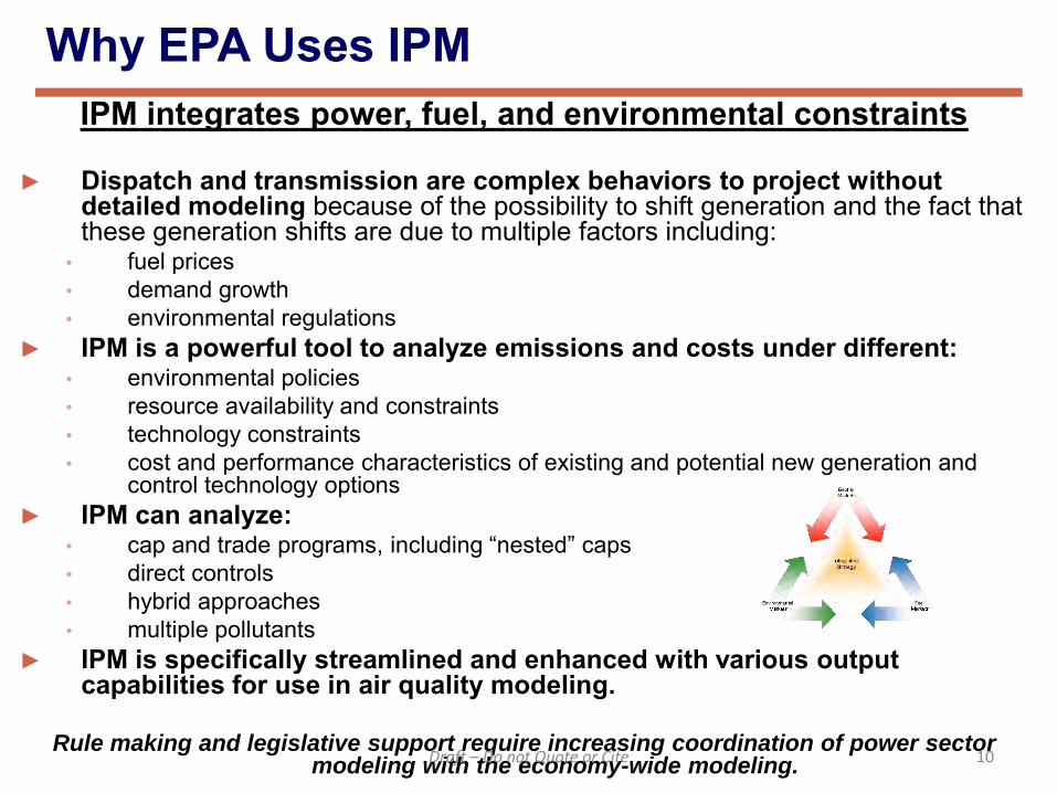
Why EPA Uses IPM

IPM integrates power, fuel, and environmental constraints

► Dispatch and transmission are complex behaviors to project without detailed modeling because of the possibility to shift generation and the fact that these generation shifts are due to multiple factors including:

• fuel prices • demand growth • environmental regulations

► IPM is a powerful tool to analyze emissions and costs under different: • environmental policies • resource availability and constraints • technology constraints • cost and performance characteristics of existing and potential new generation and

control technology options ► IPM can analyze:

• cap and trade programs, including “nested” caps • direct controls • hybrid approaches • multiple pollutants

► IPM is specifically streamlined and enhanced with various output capabilities for use in air quality modeling.

Rule making and legislative support require increasing coordination of power sector

modeling with the economy-wide modeling.


EPA’s Use of IPM ► EPA uses ICF’s Integrated Planning Model (IPM) to analyze

environmental policies affecting power sector emissions. ► EPA develops and maintains its own datasets for use in the application of IPM to

project the emissions and other impacts of environmental policies on the U.S. electric power sector.

► IPM outputs are used in EPA’s air quality models, streamlined with post-processing tools to generate unit level emissions of SO2, NOX, CO2, Hg, HCl (and PM, VOC, NH3).

► EPA’s application of IPM is used on air pollution regulations (e.g., CAIR, CSAPR, and MATS), including those dating back to the Title IV acid rain and NOX SIP call regulations, and for analysis including multi-pollutant and climate legislation

► Other clients of IPM include: ► Government agencies (FERC, RPO/MJOs, RGGI, MGA) ► Industry groups (EPRI, EEI, SoCal, PacifiCorp, TVA, AEP Florida Power, Cinergy,

National Coal Association) ► Other organizations (Center for Clean Air Policy, Clean Air Task Force, Clean Energy

Group)


EPA’s Application of IPM ► This graphic was obtained from ICF International

12 This graphic was obtained from ICF International Draft – Do not Quote or Cite

EPA Base Case Documentation ► New full-fledged documentation becomes available with each major EPA Base Case update.


Model Structure

► IPM has a linear “objective function” ► A series of “decision variables,” and ► A set of linear “constraints”

► Linear “objective function”:

► Minimize the total, discounted, net present value of the costs of meeting demand, power operation constraints, and environmental regulations over the entire planning horizon

► The sum of all the costs incurred by the electricity sector, expressed as the net present value of all the component costs (include the cost of new plant and pollution control construction, fixed and variable operating and maintenance costs, and fuel costs)

► Cost components are captured by multiplying the decision variables by a cost coefficient

► Cost escalation factors are used to reflect changes in cost over time ► Discount rates are applied to derive the net present value for the entire

planning horizon from the costs obtained for all years in the planning horizon


Model Structure

► IPM has a series of “decision variables,” which it “solves for” ► Decision variables are the model’s “outputs” and represent the optimal least-

cost solution for meeting the assumed constraints ► Key decision variables

• Generation Dispatch: Representing the generation from each model power plant, for each possible combination of fuel, season, model run year, and segment of the seasonal load duration curve applicable to the model plant

• Capacity: Representing the capacity of each existing model plant and capacity additions associated with potential (new) units in each model run year

• Transmission: Electricity transmission along each transmission link between model regions in each run year

• Emission Allowance: For emission policies where allowance trading applies, representing the total number of emission allowances that are bought and sold in current or subsequent run years

• Fuel Decision: For each type of fuel and each model run year, IPM defines decision variables representing the quantity of fuel delivered from each fuel supply region to model plants in each demand region

► Model plants are aggregate representations of real life electric generating units, used by IPM to model the electric power sector

15


Model Structure

► A set of linear “constraints” ► Reserve Margin: Regional. If existing plus planned capacity is not enough to

satisfy the annual regional reserve margin requirement, the model will “build” the required level of new capacity

► Demand: The model categorizes regional annual electricity demand into seasonal load segments and load duration curves (LDC)

► Capacity Factor: Specifies how much electricity each plant can generate (a maximum generation level), given its capacity and seasonal availability

► Turn Down: Takes into account the cycling capabilities of units ensuring that the model reflects the distinct operating characteristics of peaking, cycling, and base load units

► Emissions: An array of emission constraints for SO2, NOX, Hg, and CO2 can be implemented on a plant-by-plant, regional, or system-wide basis

► Transmission: Simultaneously models any number of regions linked by transmission lines

► Fuel Supply: Defines the types of fuel that each model plant is eligible to use and the supply regions that are eligible to provide fuel to each specific model plant. A separate constraint is defined for each model plant.


Model Structure

► Key Methodological Features of IPM IPM is a flexible modeling tool for obtaining short- and long-term

projections of production activity in the electric generation sector. The projections obtained using IPM are not statements of what

will happen but what might happen given the assumptions and

methodologies used.

► Model plants • Existing • Retrofit and retirement options • Potential (new) units

► Model run years ► Cost accounting ► Modeling wholesale electric markets ► Load Duration Curves (LDC) (see following slides)


Model Structure, cont.

18

► Hypothetical chronological hourly load curve and seasonal load duration curve in IPM



19

► Stylized depiction of load duration curve used in IPM



► Key Methodological Features of IPM, cont. ► Resource Adequacy: Specifies the amount of installed capacity

that must be in excess of peak power demand ► Fuel Modeling: Includes cost, supply, and characteristics of each

fuel ► Transmission: Detailed representation of existing transmission

capabilities between model regions ► Perfect Competition and Perfect Foresight: For wholesale

electric markets model assumes perfect competition and the entire modeling horizon has been solved simultaneously

► Air Regulatory Modeling: Detailed and flexible modeling of air regulations endogenously


Inputs ► Very detailed bottom up representation of U.S. power market regions

► NEEDS (National Electric Energy Data System) database: Each electric

generating unit’s characteristics and emission controls (more on slide 19) ► Demand, load, transmission, resource adequacy

► Coal supply

► Numerous coal grades ► Numerous coal supply and demand regions

► Natural gas module

► Numerous supply and demand regions, LNG import/export and gas storage facilities, and pipeline import/export points

► New capacity (conventional and renewable) and pollution control cost,

performance, and financing assumptions


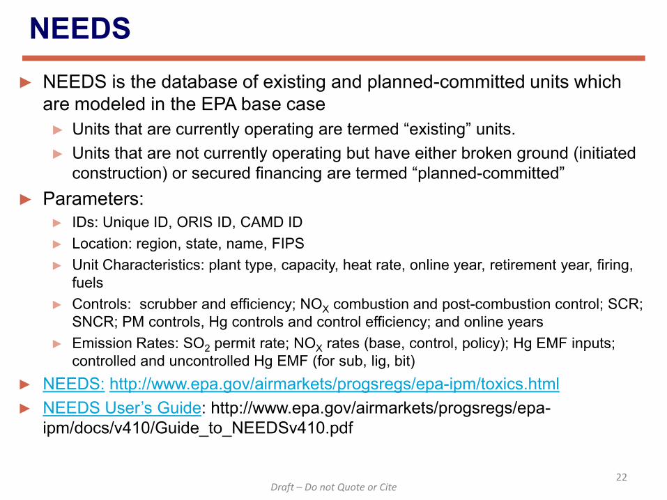
NEEDS ► NEEDS is the database of existing and planned-committed units which

are modeled in the EPA base case ► Units that are currently operating are termed “existing” units. ► Units that are not currently operating but have either broken ground (initiated

construction) or secured financing are termed “planned-committed” ► Parameters:

► IDs: Unique ID, ORIS ID, CAMD ID ► Location: region, state, name, FIPS ► Unit Characteristics: plant type, capacity, heat rate, online year, retirement year, firing,

fuels ► Controls: scrubber and efficiency; NOX combustion and post-combustion control; SCR;

SNCR; PM controls, Hg controls and control efficiency; and online years ► Emission Rates: SO2 permit rate; NOX rates (base, control, policy); Hg EMF inputs;

controlled and uncontrolled Hg EMF (for sub, lig, bit) ► NEEDS: http://www.epa.gov/airmarkets/progsregs/epa-ipm/toxics.html ► NEEDS User’s Guide: http://www.epa.gov/airmarkets/progsregs/epa-

ipm/docs/v410/Guide_to_NEEDSv410.pdf


http://www.epa.gov/airmarkets/progsregs/epa-ipm/toxics.html




http://www.epa.gov/airmarkets/progsregs/epa-ipm/docs/v410/Guide_to_NEEDSv410.pdf

Current Inputs ► The input assumptions for the EPA Base Case Application of IPM reflect the latest

available data, not a single year, obtained from numerous sources.

Draft EPA Base Case v.5.13 using IPM (there will be further updates in final) ► NEEDS

► Existing units (2010 EIA 860) ► Committed units with online year of 2015 or earlier (2010 EIA 860, AEO 2012, EPA research and

new entrants from Ventyx, 04/2012) ► Announced Coal Retirements (01/2013) ► Existing unit controls based on CAMD data (ETS 2011), 2010 EIA 860, previous versions of

NEEDS, comments received during the last 2 years, and other research ► NOx rates (CAMD data: ETS 2011) ► SO2 control removal efficiencies (2010 EIA 860) ► Heat rates for existing units (AEO 2012 and EIA Form 923) ► Nuclear unit capacity (AEO 2012)

► State Rules, Settlements, Consent Decrees ► Updated as of October, 2012 based on comments from states

► Electricity Demand: AEO 2013 ► Coal Market Assumptions: 2012-2013 update

► Numerous coal grades ► Numerous coal supply and demand regions

► Gas Market Assumptions: 2013 update ► New generation (conventional and renewable) and retrofit technology cost and

performance: AEO 2012-13 and other latest EPA assessments


Data Parameters for Model Inputs

► Electric System ► Existing utility generating resources

• Plant capacities (2010 EIA 860) • Heat rates (AEO 2012 and EIA Form 923) • Availability (AEO 2012 and NERC GADS) • Minimum generation requirements (ICF) • Fuels Allowed (EIA Forms) • Fixed and variable O&M costs (FERC Form 1 and ICF) • Emission limits or emission rates for NOx, SO2, CO2, Hg (2011 ETS, EIA) • Existing pollution control equipment and retrofit options (2011 ETS, Industry research and

EPA Assessments) ► New generating resources

• Cost and operating characteristics (AEO 2012 and EPA) • Technology Feasibility (EPA 2013)

► Other system requirements • Inter-regional transmission capabilities (Various NERC and ISO/RTO reports) • Reserve margin requirements for reliability (NERC 2012) • System specific generation requirements • Regional specification (ICF 2012/2013)

24


Data Parameters for Model Inputs, cont.

► Economic Outlook ► Electric demand

• Regional electric demand (AEO 2013 ER) • Load curves (2007 FERC Form 714)

► Financial outlook • Capital charge rate (ICF 2012) • Discount rate (ICF 2012)

► Fuels ► Coal Market Assumptions (EPA 2012/2013)

► Gas Market Assumptions (AEO 2012)

► Biomass Supply Curves (AEO 2012)

► Air Regulatory Outlook ► Air regulations for NOx, SO2, CO2, Hg ► Other EGU regulations (ash, water, as they become on the books)

25

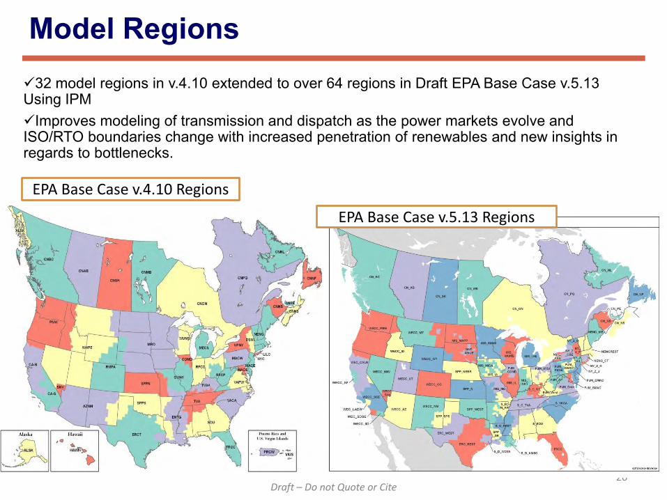
Model Regions

►

26

32 model regions in v.4.10 extended to over 64 regions in Draft EPA Base Case v.5.13 Using IPM Improves modeling of transmission and dispatch as the power markets evolve and ISO/RTO boundaries change with increased penetration of renewables and new insights in regards to bottlenecks.

EPA Base Case v.5.13 Regions

EPA Base Case v.4.10 Regions


Technology Options in EPA Base Case

► Generation Types: ► Biomass, coal steam, combined cycle, combustion turbine, fossil waste,

geothermal, hydro, IGCC, landfill gas, municipal solid waste, non-fossil waste, nuclear, O/G steam, pumped storage, solar, wind

► Retrofits:

► Dry and wet FGD, DSI, ACI, SCR, SNCR, FF (baghouse), CCS • State-of-the-art Low NOx burner.


Natural Gas Modeling

► EPA Base Case using IPM includes endogenous modeling of the North American natural gas supply system

28

Not all LNG nodes are shown

Gas Transmission Network Map

Canadian Arctic and Alaskan Supply Regions not shown

Gas Supply Regions


Natural Gas Modeling, cont. ► Draft EPA Base Case v.5.13 Using IPM has increased natural gas resource

availability

29

(1) Cove Point

(2) Elba Island

(3) Everett

(14) NE Gateway

(4) Gulf Gateway

(5) Lake Charles

(6) Altamira

(7) Costa Azul

(8) Cameron LNG

(10) Golden Pass

(9) Freeport LNG

(11) Canaport

(12) Sabin Pass

(13) Gulf LNG Energy

Existing Potential

North American LNG Regasification Facilities

7 7

7

7

7

3

8

10

7

20-Day80-DayOver 80 DaysLNG Peak Shaving

Natural Gas Storage Facility Nodes


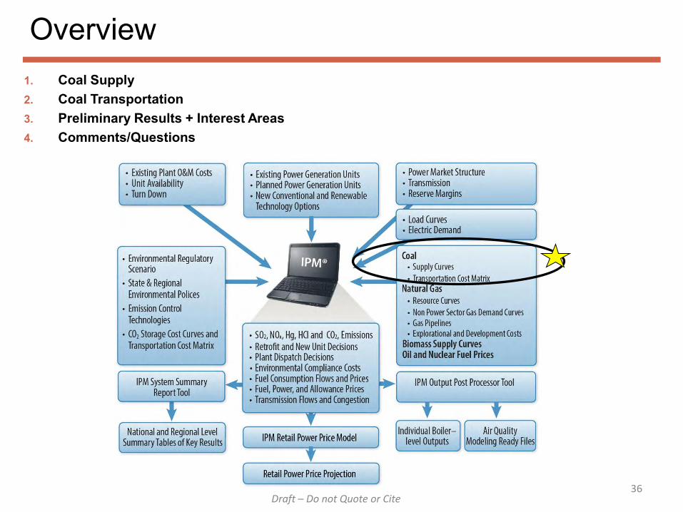
Coal Supply

30

Draft EPA Base Case v.5.13 using IPM includes detailed coal transportation matrix simulating each plant’s coal choices.


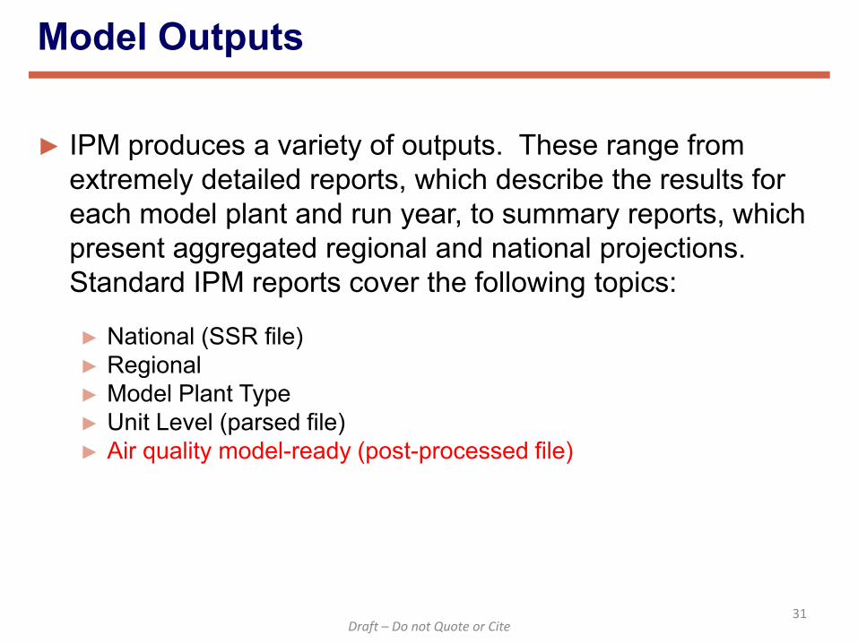
Model Outputs

► IPM produces a variety of outputs. These range from extremely detailed reports, which describe the results for each model plant and run year, to summary reports, which present aggregated regional and national projections. Standard IPM reports cover the following topics:

► National (SSR file) ► Regional ► Model Plant Type ► Unit Level (parsed file) ► Air quality model-ready (post-processed file)

31


Model Outputs, cont.

► Generation ► Capacity mix (by plant type and presence or absence of

emission controls) ► Capacity additions and retirements ► Capacity and energy prices ► Power production costs (capital, VOM, FOM, and fuel costs) ► Fuel consumption ► Fuel supply and demand ► Fuel prices for coal, natural gas, and biomass ► Emission allowance prices ► Unit-level emissions (NOX, SO2, CO2, HCl, and Hg) ► Additional post-processed emissions with stack parameters

(PM, VOC, NH3)


Model Outputs, cont ► SSR File: contains system-wide power sector results for the lower continental

U.S. for each run year. ► Reports projected generation, capacity, capacity additions, capacity factors, production costs,

emissions, fuel consumption & cost, and allowance prices by model run year at the national level and model plant type.

► Also provides information on the various regulatory and legal requirements that were input to the model as constraints.

► Example SSR file: http://www.epa.gov/airmarkets/progsregs/epa-ipm/toxics.html

► Parsed File: approximates the EPA Application of IPM results at the generating unit level

► Example Parsed File: http://www.epa.gov/airmarkets/progsregs/epa-ipm/transport.html

► Parsed File User Guide: http://www.epa.gov/airmarkets/progsregs/epa-ipm/docs/v410/Guide_to_Parsed_File_v410.pdf

► Guide to IPM Output Files: http://www.epa.gov/airmarkets/progsregs/epa-ipm/docs/v410/Guide_to_IPMv410_Input_and_Output_Files.pdf

► Air Quality Modeling-Ready Files: SMOKE-ready files are generated by a streamlined and automated post-processing tool using the parsed file. Contain unit level (lat-lon based) stack parameters and emissions of SO2, NOX, CO2, HCl, Hg (speciated) , PM2.5, PM10, VOC and NH3. PM emissions are calculated based on filterable and condensable components.



http://www.epa.gov/airmarkets/progsregs/epa-ipm/transport.html

http://www.epa.gov/airmarkets/progsregs/epa-ipm/docs/v410/Guide_to_Parsed_File_v410.pdf



http://www.epa.gov/airmarkets/progsregs/epa-ipm/docs/v410/Guide_to_IPMv410_Input_and_Output_Files.pdf



Contact Information

► CAMD website: http://www.epa.gov/airmarkets/

► EPA’s Application of IPM Website: http://www.epa.gov/airmarkets/progsregs/epa-ipm/ ► [email protected], 202-343-9390.

34

http://www.epa.gov/airmarkets/

http://www.epa.gov/airmarkets/

http://www.epa.gov/airmarkets/progsregs/epa-ipm/




mailto:[email protected]


Coal Supply and Transportation

May 3, 2013 by



Overview 1. Coal Supply 2. Coal Transportation 3. Preliminary Results + Interest Areas 4. Comments/Questions


Key Questions to Keep in Mind

1. Are there demand-side limitations impacting Illinois Basin growth?

2. What costs are associated with increasing a plant’s subbituminous or bituminous burn percentage above historic levels?

3. What is the role of PRB coal in a post 2015 world?

4. Where are coal steam export markets headed?

5. What are the obstacles to biomass co-firing at power plants?


Coal Overview

38

0

100

200

300

400

500

600

Mill

ion

to

ns

U.S. Thermal Coal Production

Powder River Basin

Central Appalachia

Illinois Basin

Northern Appalachia

Source: American Coal Foundation

Pollution Content By Coal Type (clustered values)

SO2 (lbs/MMBtu)

CO2 (lbs/MMBtu)

Hg (lbs/TBtu)

HCL (lbs/MMBtu)

Bituminous 0.66– 7.27 202 - 210 1.8 - 26 0.005 - .28

Subbituminous 0.6 – 1.9 209 - 215 2.0 – 8.6 0.001 - 0.003

Lignite 1.5 – 3.9 212 - 219 7.5 – 14.9 0.003 – 0.009


Source: Wood Mackenzie

Source: Platts Coal Trader

0

0.5

1

1.5

2

2.5

3

Northern App Central App Illinois Basin PRB

$/MMBtu

Coal Supply Curves

39

►EPA collaborates with Wood Mackenzie for bottom-up, mine-based supply curve development

Steps 1. Identify mines (approximately 1,700) 2. Map mines to supply regions and coal grades 3. Assign emission factors to each coal type 4. Identify new mines & cost escalation 5. Group similar mines within a region into “steps”

North Antelope Surface Mine - Wyoming

North River Underground Mine - Alabama


Coal Supply – Mine Identification, Rank/Grade

40

Mine State Strip Ratio Railroad

Heat Content (Btu/lb) Ash % Sulphur %

2010 Production

Capacity (t/y)

Cash Cost 2011$

Mine Reserves

(million tons)

TWILIGHT WV 17 CSX 12,600 10.5 0.69

3,168,486

3,487,452 59.2 78.9

Step 1 – Identify individual mines and characteristics

Cash Cost – Direct operating cost – labor, materials, overhead, pensions, transportation to point-of-sale Other – royalties, severance taxes, black lung fees, property tax, reclamation tax

Production Capacity - based largely on Wood Mackenzie proprietary data; also MSHA data Reserves – • Environmental Impact Statements • SEC filings • USGS data on seam thickness and coal depth • Interviews with company personnel • Checked to ensure they do not exceed EIA’s “Demonstrated Reserve Base” Draft – Do not Quote or Cite

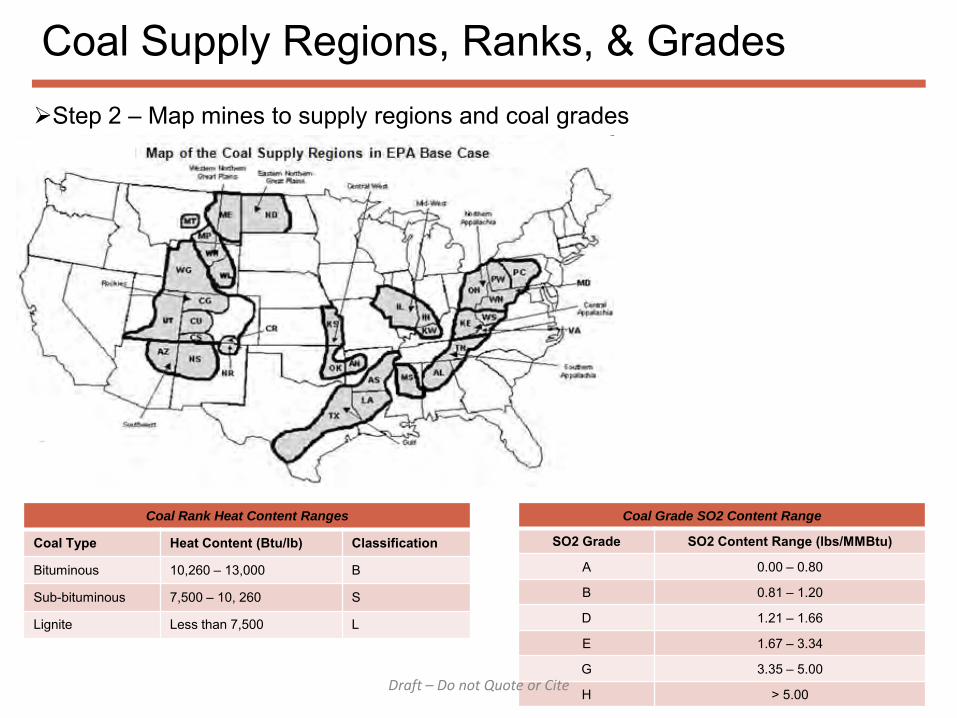
Coal Supply Regions, Ranks, & Grades

41

Step 2 – Map mines to supply regions and coal grades

Coal Rank Heat Content Ranges

Coal Type Heat Content (Btu/lb) Classification

Bituminous 10,260 – 13,000 B

Sub-bituminous 7,500 – 10, 260 S

Lignite Less than 7,500 L

Coal Grade SO2 Content Range

SO2 Grade SO2 Content Range (lbs/MMBtu)

A 0.00 – 0.80

B 0.81 – 1.20

D 1.21 – 1.66

E 1.67 – 3.34

G 3.35 – 5.00

H > 5.00 Draft – Do not Quote or Cite

Coal Supply – Quality and Emissions

42

Coal Supply Region Coal Grade

Heat Content (MMBtu/ton)

SO2 Content (lbs/MMBtu

Hg Content (lbs/Tbtu)

Ash Content (lbs/MMBtu)

CO2 Content

(lbs/MMBtu) HCL Content (lbs/MMBtu)

PC

BD 25.55 1.4 5.7 10.3 206 .027

BE 25.24 2.68 12.6 7.1 205 .027

BG 25.33 3.8 21.5 9.6 205 .0923

PW BE 26.22 2.5 8.4 5.4 204 .206

BG 25.86 3.7 8.6 6.5 205 .059

Use ICR and EIA data to identify coal

characteristics for each region/grade

combination

Clustering algorithm used to further aggregate data for

model size management

Step 3 – Derive emission factors for each coal type


Coal Supply – Future Mines, Future Cost

New mines – based on announced projections, coal lease applications, and unassigned reserves Mine productivity – function of projected production, stripping ratios, rising raw material costs

43

Step 4 – Identify new mines, productivity changes, and cost escalation

0.0%

0.5%

1.0%

1.5%

2.0%

2.5%

3.0%

Annual Basin-level Cost Escalation


EPA IPM Supply Curves

44

-

50

100

150

200

250

- 5 10 15 20 25 30 35 40 45

WS BD Coal Supply (million tons)

2016

2020

2025

2030

2040

2050

Year Coal Supply

Region Coal Grade Step Name Heat Content (MMBtu/ton)

Cost of Production (2011$/ton)

Production Capacity (Million

tons)

Cumulative Production (Million

tons)

End 2015 Coal Reserves (Million

tons)

2016 WS BD E1 24.40 27.51 0.13 0.13 1.70

2016 WS BD E2 24.50 33.86 0.32 0.45 11.80

2016 WS BD E3 24.50 48.58 4.50 4.95 30.42

2016 WS BD E4 24.50 58.36 15.37 20.32 268.19

2016 WS BD N2 24.40 61.56 0.30 20.62 20.00

2016 WS BD E5 24.50 68.56 10.49 31.11 271.96

2016 WS BD N3 24.40 79.60 1.00 32.11 500.00

2016 WS BD E6 24.50 80.76 6.86 38.96 141.69

2016 WS BD E7 24.50 105.62 1.56 40.52 35.35

2016 WS BD E8 24.50 132.66 0.08 40.60 5.42

WS BD Coal Characteristics

SO2 content – 1.3 lb/MMBtu Hg content – 8.1 lb/MMBtu HCL content - .097 lb/MMBtu CO2 content – 206.4 lb/MMBtu

Step 5 - Group similar mines into steps. Sort cost by ascending order.


Supply Curves for Major Basins

45

$0

$10

$20

$30

$40

$50

$60

$70

$80

$90

$100

Million tons

Illinois Basin

$0

$20

$40

$60

$80

$100

$120

$140

$160

$180

$200

Million tons

Northern App Basin

$0

$10

$20

$30

$40

$50

$60

$70

Million tons

Powder River Basin


$0

$50

$100

$150

$200

$250

$300

$350

Million tons

Central App Basin

Basin-level Production Caps and Reserve Depletion

46

$0

$10

$20

$30

$40

$50

$60

$70

Million tons

PRB 2016

$0

$10

$20

$30

$40

$50

$60

$70

Million tons

PRB 2050

Reserves depleted Max production capacity = 594.5

$0

$10

$20

$30

$40

$50

$60

$70

Million tons

PRB 2040

Max production capacity = 594.5

Table 2: Reserve Depletion

Coal Supply Region Coal Grade

Step Name

Coal Production (Million tons/year)

End 2015 Coal Reserves

(Million tons) WL SB 1 95 1,900 MP SD 2 15 450 WL SB 3 19 345 MP SA 4 30 777 MP SD 5 15 162

Table 1: Maximum Production Capacity by Year (Million tons) 2016 2020 2025 2030 + PRB 509.0 552.5 572.3 594.5 Illinois Basin 165 203 286 315 Max production capacity = 509

Step 1,3,5 Reserve - Depleted


$0

$20

$40

$60

$80

$100

$120

$140

$160

0 10 20 30 40 50 Million tons

2020 Southern WV BD coal

Price = Marginal Cost

Year Coal Supply

Region Coal

Grade Step

Production Capacity

(Million tons per year

Cumulative Production

(million tons)

Cost of Production

(2011$/short ton)

2020 WS BD 1 0.13 0.13 29.20

2020 WS BD 2 0.32 0.45 35.94

2020 WS BD 3 4.50 4.95 51.56

2020 WS BD 4 15.37 20.32 61.95

2020 WS BD 5 0.30 20.62 65.34

2020 WS BD 6 10.49 31.11 72.77

2020 WS BD 7 1.00 32.11 84.49

2020 WS BD 8 6.86 38.96 85.71

2020 WS BD 9 1.56 40.52 112.10

2020 WS BD 10 0.08 40.60 140.80

47

Draft EPA Base Case v.5.13 Using IPM – Output File (RPT)

On step

Off step

Draft EPA Base Case v.5.13 Using IPM – Input File


Stream Name Fuel Produced (million tons) Step Cost ($/ton)

Step Cost ($/MMBtu)

Marginal Price ($/MMBtu)

Marginal Price ($/ton)

Coal BD from West Virginia, South - 1 0.13 29.20 1.19 2.77 67.89

Coal BD from West Virginia, South – 2 0.32 35.94 1.47 2.77 67.89




48

Coal Transportation


Coal Transportation

► Transportation links established individually for each of the approximately 500 coal plants

► Based on historic deliveries ► Based on potential for new supplies to reach plant

► On average, each coal plant in Draft EPA Base Case v.5.13 has 9 transportation links

49

Plant Name Plant State

Coal Supply

Region

Coal Supply Region

Description

Total Cost (2012

Rate in

2011$/Ton)

Escalation/Year

(2013-2025)

Conemaugh PA KE Kentucky East $29.38 1.005

Conemaugh PA MD Maryland $17.90 1.005

Conemaugh PA OH Ohio $14.04 1.005

Conemaugh PA PC Pennsylvania, Central $7.00 1.004

Conemaugh PA PW Pennsylvania, West $12.60 1.005

Conemaugh PA WN West Virginia, North $13.68 1.005

Conemaugh PA WS West Virginia, South $28.86 1.005


Transportation Routings & Coal Origin Points

► Modeling each coal plant as a demand region allows us to capture specific railway serving that plant (e.g., CSX)

► To determine distance and calculate delivery costs, origin points are defined within each coal supply region

► Origin points in each supply region are based on significant mines or significant delivery points within in a coal supply region

► Multiple origin points identified for each supply region specific to major rail carriers (e.g., Norfolk Southern and CSX in East)

50

Example – Southern West Virginia Origin Points • Wells Prep Plant – CSX (rail) • Delbarton, WV – Norfolk Southern (rail) • Ceredo Dock – central hub for barge-delivered App. coal


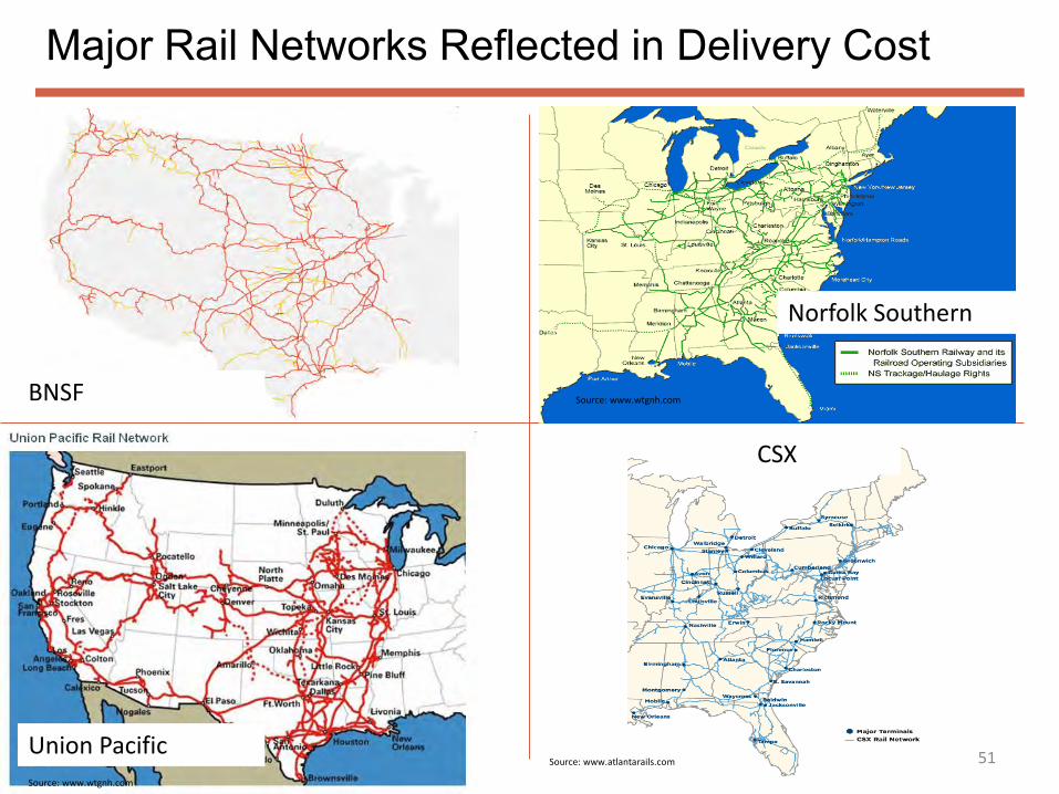
Major Rail Networks Reflected in Delivery Cost

51 Source: www.atlantarails.com

Source: www.wtgnh.com BNSF

Union Pacific

Norfolk Southern

CSX

Source: www.wtgnh.com

Rail Transport

1. Rail “origin points” identified in each supply region 2. Competition type identified 3. Determine rates per mileage block

52

Competition Type Definition

Captive

Demand source can only access coal supplies through a single provider; demand source has limited power when negotiating rates with railroads.

High-Cost Competitive

Demand source has some, albeit still limited, negotiating power with rail providers; definition typically applies to demand sources that have the option of taking delivery from either of the two major railroads in the region.

Low-Cost Competitive

Demand source has a strong position when negotiating with railroads; typically, these demand sources also have the option of taking coal supplies via modes other than rail (e.g., barge, truck, or lake/ocean vessel).

Mileage Block Captive High-Cost Competitive Low-Cost Competitive

< 200 85 85 72

200-299 71 71 60

300-399 69 69 59

400-649 61 61 52

650+ 43 43 37

Assumed Eastern Rail Rates for 2012 (2011 mills/ton-mile)


Barge Transport

53

1. Classify barge moves into three categories 2. All barge and lake vessel rates considered “competitive” because river access is

open to all barge firms 3. Rates for Great Lakes coal transport are determined on plant-specific basis

Type of Barge Movement Loading Cost ($/ton)

Transport (mills/ton-

mile) Upper Mississippi River, and Downstream on the Ohio River System

2.70 9.7

Upstream on the Ohio River System 2.45 11.5

Lower Mississippi River 2.70 6.9 Notes: 1. The Upper Mississippi River is the portion of the Mississippi River north of St. Louis. 2. The Ohio River System includes the Ohio, Big Sandy, Kanawha, Allegheny, and Monongahela Rivers. 3. The Lower Mississippi River is the portion of the Mississippi River south of St. Louis.


Trunk Cost and Transfers

54

All trucking flow is considered competitive due to open highway access

Market Loading Cost ($/ton)

Transport (mills/ton-mile)

All Markets 1.00 120

Type of Transportation Rate

($/ton) Rail-to-Barge Transfer 1.50

Rail-to-Vessel Transfer 2.00

Truck-to-Barge Transfer 2.00

Rail Switching Charge for Shortline

2.00

Conveyor 1.00

Transfer charges also apply when coal must be moved between different transportation modes


Transportation Market Drivers

► Fuel –Expected real increase of 0.8%/yr for diesel ► Equipment – Relatively stable ► Labor – Expected real increase of 1% for rail labor, no real increase for

more competitive truck and barge markets ► Productivity – some productivity gains expected for barge transportation

55

Mode ComponentComponent Weighting

Real Escalation

Before Productivity Adjustment

(%/year)

Productivity Gains Passed

Through to Shippers (%/year)

Real Escalation

After Productivity Adjustment

(%/year)

Rail Fuel 20% 0.8%Labor 35% 1.0%Equipment 45% 0.0%Total 100% 0.5% 0.0% 0.5%

Barge & Vessel Fuel 35% 0.8%Labor & Equip. 65% 0.0%Total 100% 0.3% 0.5% -0.2%

Truck Fuel 50% 0.8%Labor & Equip. 50% 0.0%Total 100% 0.4% 0.0% 0.4%

Conveyor Total 0.0% 0.0% 0.0%

Transloading Terminals Total 0.0% 0.0% 0.0%


Summary of Expected Escalation for Coal Transportation Rates

Some Key Issues Going Forward


-

100

200

300

400

500

600

Mill

ion

to

ns

Thermal Coal Export

Wood Mackenzie Long Term Outlook

AEO 2013 ER

Thermal Coal Export Demand

► Where are thermal coal export markets headed?

► WoodMac – “Export growth

largely predicated on large-scale US West Coast facilities being constructed/expanded…. A major risk is the actual construction of these new ports with environmental opposition adding risk to the permitting process. US West Coast port capacity growth of 260 Mstpa in the next 20 years represents a huge risk to our base case forecast”.

57

Assumed thermal export demand will have major impact on domestic production, assumption, and coal prices


What Limitations Are Associated With Coal Switching?

58

If increasing subbituminous • Increased cost due to material handling , milling capacity, dust control, and boiler

modifications; heat rate penalty due to higher moisture content • Plant pays a $250/KW (~$0.50/MMBtu) cost adder and a 5% heat rate penalty

If increasing bituminous The low ash fusion temperatures and/or the corrosive nature of its high chlorine content may necessitate some soot blowing and/or heat transfer surface modifications $50/KW (~$0.10/MMBtu) cost adder and 5% heat rate bonus

James H. Miller Plant (2012 consumption = 10 million tons) Delivered Cost in Future IPM Run Year (illustrative) • PRB = $2.70/MMBtu • Illinois Basin = $2.68/MMBtu


What Role Will PRB Play in 2016 and Beyond?

► Fly Ash Chemistry ► The calcium oxide in lignite and subbituminous coals provides a natural alkalinity

with a PH of 9+ that can neutralize much of the HCL in the flue gas stream ► 2010 ICR was suggesting 50% to 85% HCL removal in fly ash ► Current assumption is HCL removal at 75%. ► However, growing evidence of higher HCL removal ► At 83%, Wyoming PRB coals meet .002 MATS standard ► At 95%, lignite coals meet .002 MATS standard

59

HCL Characteristic of PRB coals

Coal Supply Region Coal

Grade Production Capacity

(million tons) % of Nationwide Subbit

production capacity HCL Content (lbs/MMBtu)

% removal needed to meet .002 lbs/mmbtu

PRB - Montana SA 23 4% 0.007 71% SD 20 3% 0.006 67%

PRB - Wyoming SA 276 45% 0.012 83% PRB - Wyoming SB 208 34% 0.012 83%


Biomass Co-firing

► Biomass co-firing provided as a fuel choice for all coal-fired units ► A maximum of 10% of facility power (not to exceed 50 MW)

• Logistical limitations – only economic to transport limited distance • Boiler considerations – high moisture content, lower heat content, storage

issues ► Significant portion of biomass co-firing driven by RPS in model ► Potential changes:

► Incorporate storage cost (e.g., ~$20/ton = $1.66/MMBtu)* ► Apply seasonal capacity factors

60

0

10

20

30

40

50

60

70

80

1000 GWh # of plants

Biomass Co-firing

2012 reported (EIA 923)

2016 Draft EPA Base Case v.5.13


0

10

20

30

40

50

60

2016 2020 2025 2030 2040

Tho

usa

nd

GW

h

Biomass Co-firing Generation

Draft EPA Base Case v.5.13

AEO 2013 ER

* Source - “Estimated Cost for Production, Storage and Transportation of Switchgrass. Iowa State University. 2008



61

Thank You


Natural Gas Framework

May 3, 2013 by

U.S. Environmental Protection Agency Office of Air and Radiation Clean Air Markets Division

Overview

► Overview of Natural Gas Module used in Draft EPA Base Case v.5.13 using IPM

► Key Components of Natural Gas Framework

► Supply Module

► Liquefied Natural Gas (LNG) Sub‐Module

► Non‐Electric Sector Natural Gas Demand Sub‐Module

► Pipeline Module

► Storage Module

► Other Modeling Algorithms

► Crude Oil and Natural Gas Liquids Prices

► LNG Exports

► Capacity Expansion Algorithm

► Supply and Demand Balance and Price Response

► IPM Natural Gas Modeling Results


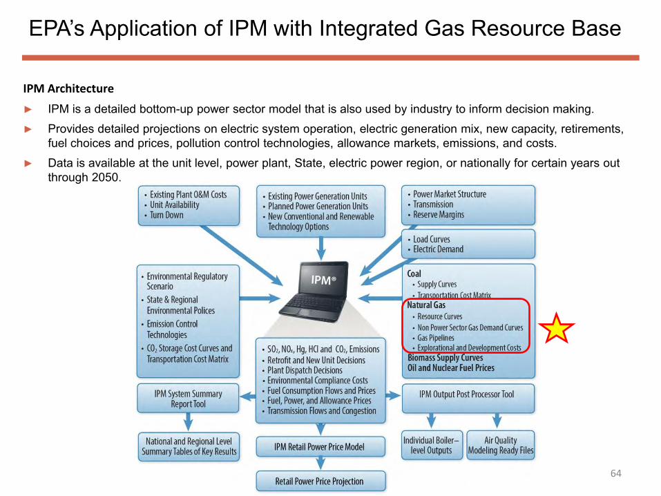
EPA’s Application of IPM with Integrated Gas Resource Base

64

IPM Architecture ► IPM is a detailed bottom-up power sector model that is also used by industry to inform decision making.

► Provides detailed projections on electric system operation, electric generation mix, new capacity, retirements, fuel choices and prices, pollution control technologies, allowance markets, emissions, and costs.

► Data is available at the unit level, power plant, State, electric power region, or nationally for certain years out through 2050.

Key Components of the Natural Gas Module


EPA’s Application of IPM with Integrated Gas Resource Base

66

Natural Gas Framework in EPA’s Application of IPM: ► 133 nodes which represent supply

regions, demand regions, LNG import/export facilities, gas storage facilities, and pipeline import/export points.

► 81 supply regions. ► 118 demand regions. Each of the gas

power plants is assigned to one of the 118 gas demand regions.

► 14 LNG regasification facilities. 1 LNG export terminal (Kitimat, BC).

► 4 U.S./Mexico pipeline import/export nodes.

► 108 underground storage facilities linked to 48 nodes. LNG peak shaving storage facilities linked to 24 nodes.

► 377 gas pipeline corridors (including bidirectional links).


Natural Gas Supply: Resource Discovery, Development, and Production


Natural Gas Resource Methodology

68

Recoverable Natural Gas Resources

(Trillion cubic feet)

AEO 2010

AEO 2011

AEO 2012

EPA 410 EPA 513

Lower 48 Onshore Non Associated 1,189 1,612 1,250 1,616 2,049 Conventional (includes tight) 740 668 646 626 566 Shale Gas 347 827 482 917 1,408

Northeast 73 473 217 254 647 Gulf Coast 90 105 130 432 492 Midcontinent 51 63 40 133 151 Southwest 60 87 46 60 67 Rocky Mountain 22 58 37 38 50 West Coast 51 41 12 0 0

Coalbed Methane 103 117 122 73 75 Lower 48 Offshore Non Associated 284 269 263 136 85 Associated-Dissolved Gas 117 135 146 143 116 Alaska 291 282 272 153 51 Total U.S. 1,881 2,299 1,931 2,048 2,300

Canada Non Associated 768 742 Canada Associated-Dissolved Gas 7 4 Total Canada 775 746 Total U.S and Canada 2,824 3,046

• Resource assumptions based initially on extensive industry participation and review of resources at the play level from the National Petroleum Council (NPC) 2003 study.

• Updated with detailed GIS assessments for unconventional gas resources provided by 22 oil and gas companies.

• The play coverage includes 24 shale plays, 18 tight gas plays, 3 conventional plays, and 6 coalbed methane plays.

• A “bottom-up” approach that first generates estimates of gas-in-place (GIP).

• Reservoir and economic models are utilized to determine well profile and well recovery of the grid cells to characterize the recoverable gas resources and economic resources.

• Resource cost curves are generated by sorting and stacking the grid cell recoverable resources based on exploration and development economics.


Natural Gas Supply Regions

69

81 supply regions


Non‐Electric Sector Natural Gas Demand Regions

70

118 demand regions. Each gas power plant is assigned to one of the 118 gas demand regions.


Non‐Electric Sector Natural Gas Demand Curves

► Non‐power sector natural gas demand (i.e. residential, commercial, and industrial) is modeled in the form of node‐level firm and interruptible demand curves.

► Calibrated to AEO 2012

► 118 demand regions in the U.S. and Canada.

► The firm demand curves are developed and used for residential, commercial, and some industrial gas customers.

► The interruptible demand curves are developed and used exclusively for industrial gas customers.

► Developed from GMM econometric demand models.

• Functions of weather, economic growth, price elasticity, efficiency and technology improvements, and other factors.

• Response function to price changes based on historical data.


Natural Gas Storage Facilities

72

108 underground storage facilities (some aggregated), linked to 48 nodes.


Natural Gas Storage Facilities (continued)

► The EPA's Application of IPM has 108 underground storage facilities that are linked to 48 nodes.

► The underground storage is grouped into three categories based on storage “Days Service”:

► “20‐Day” high deliverability storage (35 storage facilities)

► “80‐Day” depleted/aquifer reservoirs (38 storage facilities)

► “Over 80 Days” depleted/aquifer reservoirs (35 storage facilities)

► “Days Service” refers to the number of days required to completely withdraw the maximum working gas inventory associated with an underground storage facility.

► The model also includes LNG peak shaving storage facilities that are linked to 24 nodes.

► The level of gas storage withdrawals and injections are calculated within the supply and demand balance algorithm based on working gas levels, gas prices, and extraction/injection rates and costs.

► Storage working gas capacity and daily injection and withdrawal rates are specified as inputs. The model is allowed to add capacity, based on seasonal price spreads.


Crude Oil and Natural Gas Liquids Prices

► Hydrocarbon production from the exploration and development process includes crude oil and natural gas liquids (NGL).

► Revenues from crude oil and NGL production play a key role in determining the extent of exploration and development for natural gas.

► Higher crude oil/liquid prices provides an incentive for E&D activities in the liquid rich plays.

► To take into account these revenues, crude oil and NGL price projections are provided as inputs to the EPA's Application of IPM and factored into the calculation of costs in the IPM objective function.


Other Modeling Algorithms: LNG Exports

► The Draft EPA Base Case v.5.13 includes one LNG export terminal

► Kitimat LNG export terminal in British Columbia, Canada. ► The EPA's Application of IPM does not currently have a specific

sub‐module for LNG exports. ► Assumptions for exports taken from AEO 2012

► The modeling of Kitimat LNG export is currently done through firm demand.

► A new demand node is added to represent customers for Kitimat LNG export.

► The new node is linked to an existing node in British Columbia. ► A scenario based Kitimat LNG export projection is provided as input

to the new node in the form of inelastic firm demand curves.


Pipeline Capacity Expansion Algorithm

► The EPA's Application of IPM is equipped with capacity expansion algorithms for pipeline corridors, LNG regasification facilities, and gas storage facilities.

► The capacity expansions throughout the modeling horizon are treated as potential projects and are competing with each other.

► The decision to expand the capacity of the facilities is controlled by levelized capital cost of expanding the capacity and capacity constraints.

► Base year capacities, capacity constraints, and levelized capacity expansion costs are provided as inputs.

► The model can add capacity to a facility in any year, subject to capacity constraints, if the expansion cost contributes to the optimal solution, i.e., minimizes the overall costs (including the capital cost for adding new capacities) less their revenues (from oil, NGLs, and gas production).

► The model considers all possible expansion projects (pipeline corridors, LNG regasification facilities, and gas storage facilities) throughout the modeling horizon (perfect foresight) and selects the combination of expansion projects that provide the minimum objective function value.


Supply and Demand Balance and Price Response

► Natural gas prices are market clearing prices derived from the supply and demand balance at each node.

► On the supply‐side, prices are determined by production and storage price curves that reflect prices as a function of production and storage utilization.

► Prices are also affected by the “pipeline discount” curves which represent the marginal value of gas transmission as a function of a pipeline’s load factor and result in changes in basis differential.

► On the demand‐side, the price/quantity relationship in the demand curves capture the fuel‐switching behavior of end‐users at different price levels.

► The model balances supply and demand at all nodes and yields market clearing prices determined by the specific shape of the supply and demand curves at each node.


Supply and Demand Balance and Price Response




79

Thank You


Cost, Performance, and Financing of Potential Units

May 3, 2013 by



80 Draft - Do Not Quote or Cite

Introduction

► IPM is selecting from a suite of options to meet growing load and reserve requirements in a least-cost manner:

► Retrofits and increased utilization of existing resources (load only) ► New builds (load and reserve)

► Cost/performance and financial assumptions are integral to this decision ► In addition to a host of other technical and market drivers covered in this

workshop 82

0

1,000,000

2,000,000

3,000,000

4,000,000

5,000,000

6,000,000

2012 2017 2022 2027 2032 2037

Pro

ject

ed N

et D

eman

d (

GW

h)

Retrofit/Retire/New Build Increased Utilization/New Build

Draft - Do Not Quote or Cite

New Build Cost and Performance

83


New Build Orientation

► The cost and performance assumptions for new build options in EPA’s Draft Base Case v.5.13 are based primarily on EIA’s AEO2012

► Supplemented by EPA’s expert judgment ► There are two basic categories of new potential build types:

1. Conventional (fossil and nuclear) 2. Renewable (dispatchable and non-dispatchable)

84


Conventional Technologies Cost and Performance

► EPA does not make a distinction between ‘bituminous’ and ‘subbituminous’ coal build types.

► EPA does not model different vintages of conventional build types.

85

Build Type Capital Cost (2011$/kW)

Fixed O&M (2011$/kW-yr)

Variable O&M (2011$/MWh)

Heat Rate (btu/kWh)

Combined Cycle 1,025 14.9 3.2 6,430

Combustion Turbine 680 6.8 10.1 9,750

Nuclear 5,449 90.6 2.1 10,460

IGCC 3,289 49.9 7.0 8,700

SCPC* 2,905 30.3 4.3 8,800

Advanced Coal + CCS 5,462 70.8 8.2 10,700

* SCPC cost and performance is considered to generally reflect new CFB build options.


From Base Costs to Regional Costs

► There are several steps between the total overnight costs (TOC) displayed in the previous slide and the regional capital costs that IPM utilizes to solve for a least-cost solution in the model run.

86

TOC • Inclusive of project/process contingencies and

owner’s costs

TASC • Interest during construction (IDC) applied to

calculate ‘all-in’ or total as-spent cost (TASC)

Regional TASC

• Cost scalars are applied by region and technology

• Cost scalars by technology are new for v5.12

Effective TASC

• Short-term capital cost adders

• Learning rates


Interest During Construction

► IDC is added to the overnight costs of the project and is a function of lead time, construction profile, and the technology’s discount rate.

87

Plant type Lead Time

(Years)

Construction Profile

Year 1 Year 2 Year 3 Year 4 Year 5 Year 6

Coal 4 0.15 0.3 0.4 0.15 0 0

Gas 2 0.35 0.65 0 0 0 0

Nuclear 6 0.05 0.1 0.25 0.3 0.2 0.1

Wind 3 0.05 0.1 0.85 0 0 0

Offshore Wind 4 0.05 0.1 0.3 0.55 0 0

Solar Thermal 3 0.15 0.4 0.45 0 0 0


Capital Cost Multipliers

88

Capacity Type Minimum Regional Scalar Maximum Regional Scalar

Pulverized Coal 0.885 1.326

IGCC 0.908 1.284

Advanced Coal w/CCS 0.906 1.268

Combustion Turbine 0.932 1.684

Combined Cycle 0.893 1.664

Nuclear 0.954 1.136

Wind 0.947 1.246

Offshore Wind 0.918 1.294

Solar Thermal 0.824 1.501

Solar PV 0.841 1.449

► Capital cost multipliers reflect regional differences in labor, material, and construction costs.

► The range in regional scalars for selected technology types are presented below:


Short-Term Cost Adders and Learning Rates

► Cost adders are applied to a specific technology type if incremental builds in a run year exceed specified bounds.

► The increase in cost represents competition for scarce labor and resources driving up prices; therefore, the price increase is applied to all builds – not just the portion that exceeds the initial cost step.

► For example, below are representative cost adder steps for combustion turbine builds:

► Learning rates are determined by EPA’s capacity expansion projection; learning cost improvements are applied at the component level on a range from revolutionary to mature.

► Representative of learning by doing.

89

CT Builds - 2020 Step 1 Step 2 Step 3

Bound (MW) 120,492 80,328 Always Unlimited

Adder ($/kW) 0 213 551


Renewable Technologies Cost and Performance (2016)

90

Build Type Capital Cost (2011$/kW)

Fixed O&M (2011$/kW-yr)

Variable O&M (2011$/MWh)

Heat Rate (btu/kWh)

Wind 2,612 28.7 0 NA

Offshore Wind 5,978 54.5 0 NA

Solar PV 3,689 17.06 0 NA

Solar Thermal 4,216 65.4 0 NA

Biomass 3.942 102.7 5.11 13,500

Landfill Gas – High 8,408 381.7 8.51 13,648

Landfill Gas – Low 10,594 381.7 8.51 13,648

Landfill Gas – Very Low 16,312 381.7 8.51 13,648

Geothermal 2,219-29,459 87-938 0 30,000

Fuel Cell 7,118 357.5 0 9,038


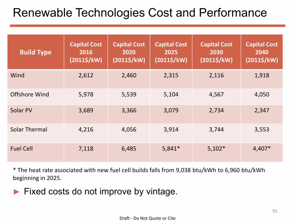
Renewable Technologies Cost and Performance

91

Build Type Capital Cost

2016 (2011$/kW)

Capital Cost 2020

(2011$/kW)

Capital Cost 2025

(2011$/kW)

Capital Cost 2030

(2011$/kW)

Capital Cost 2040

(2011$/kW)

Wind 2,612 2,460 2,315 2,116 1,918

Offshore Wind 5,978 5,539 5,104 4,567 4,050

Solar PV 3,689 3,366 3,079 2,734 2,347

Solar Thermal 4,216 4,056 3,914 3,744 3,553

Fuel Cell 7,118 6,485 5,841* 5,102* 4,407*

► Fixed costs do not improve by vintage.

* The heat rate associated with new fuel cell builds falls from 9,038 btu/kWh to 6,960 btu/kWh beginning in 2025.


Renewable Capacity Cost Declines

-

2,000

4,000

6,000

8,000

2016 2020 2025 2030 2040

Cap

ital

Co

st (

20

11

$/k

W) Fuel Cell

Offshore Wind

Solar Thermal

Solar PV

Wind

92

0%

10%

20%

30%

40%

% Decrease (2016-2040)

% D

ecr

eas

e in

Cap

ital

C

ost

(2

01

6-2

04

0) Fuel Cell

Offshore Wind

Solar Thermal

Solar PV

Wind


Capital Cost Vintages

► Select renewable build types are defined by multiple capital cost vintages, representing expected technology improvements.

► Capital cost declines associated with newer vintages occur independent of IPM’s capacity expansion projections.

► The establishment of vintages is unique to certain renewable capacity types in EPA’s Draft Base Case v.5.13; AEO2012 applies vintage improvements more broadly to conventional (including heat rate) and renewable capacity types.

► EPA is continually evaluating how the uncertainty surrounding long-term capital costs is portrayed in its Base Case.

93


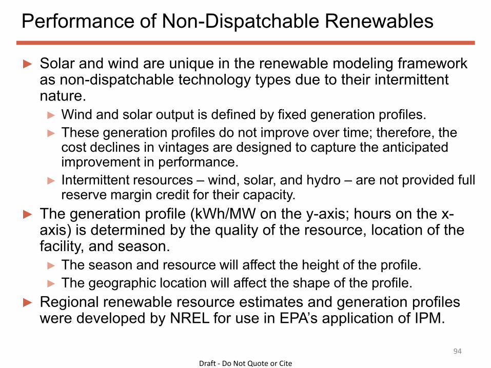
Performance of Non-Dispatchable Renewables

► Solar and wind are unique in the renewable modeling framework as non-dispatchable technology types due to their intermittent nature.

► Wind and solar output is defined by fixed generation profiles. ► These generation profiles do not improve over time; therefore, the

cost declines in vintages are designed to capture the anticipated improvement in performance.

► Intermittent resources – wind, solar, and hydro – are not provided full reserve margin credit for their capacity.

► The generation profile (kWh/MW on the y-axis; hours on the x-axis) is determined by the quality of the resource, location of the facility, and season.

► The season and resource will affect the height of the profile. ► The geographic location will affect the shape of the profile.

► Regional renewable resource estimates and generation profiles were developed by NREL for use in EPA’s application of IPM.

94


NREL Wind Resource

95

► Wind resources are grouped into: 1. Resource classes 2. Cost steps

► Resource classes are defined by wind speed; EPA’s application of IPM models wind classes 3-7.

► Wind classes are further categorized by cost step (1-4), reflecting factors such as distance from transmission, topography, population density, etc.

► Step 1: 1.0x capital cost ► Step 2: 1.2x capital cost ► Step 3: 1.5x capital cost ► Step 4: 2.5x capital cost


Representative Wind Generation Profiles

► Wind generation profiles were developed with regional data from NREL.

► Regional variation will affect the shape of the profile.

► Wind class will affect the height of the profile

► Average annual capacity factors by wind class (onshore/shallow offshore) are:

► Class 3: 29/31% ► Class 4: 33/34% ► Class 5: 39/41% ► Class 6: 46/48% ► Class 7: 50/52%

96

0

100

200

300

400

500

600

1 2 3 4 5 6 7 8 9 10 11 12 13 14 15 16 17 18 19 20 21 22 23 24

kWh

/MW

Hour of Day

Representative Wind Generation Profile (Winter)

Class 3 Class 4 Class 5 Class 6 Class 7

0

100

200

300

400

500

600

1 2 3 4 5 6 7 8 9 10 11 12 13 14 15 16 17 18 19 20 21 22 23 24

kWh

/MW

Hour of Day

Representative Wind Generation Profile (Summer)

Class 3 Class 4 Class 5 Class 6 Class 7


Overview of Solar Resources

► NREL also developed solar generation profiles for use in EPA’s application of IPM regions:

► Similar to wind, solar thermal resources are divided by class.

► Photovoltaic resources vary by region, not class.

► A notable update to EPA’s Draft Base Case v.5.12 representation of solar build options is the introduction of resource limits for both CSP and PV.

97

United States Solar PV Resource

United States Solar Thermal Resource


Solar Capacity Factors

► The generation profiles shown to the right are representative of the Arizona region in EPA’s Draft Base Case v.5.13.

► The average annual capacity factors associated with CSP resources are more tightly grouped than wind.

► CSP Class 2: 39.2% ► CSP Class 3: 42.7% ► CSP Class 4: 43.3% ► CSP Class 5: 44.7%

► The average annual capacity factor for PV in the Arizona region is 26.3%.

98

0

500

1000

1500

kWh

/MW

Representative Solar Generation Profile (Winter)

CSP Class 2 CSP Class 3 CSP Class 4

CSP Class 5 PV

0

500

1000

1500

2000 kW

h/M

W

Representative Solar Generation Profile (Summer)


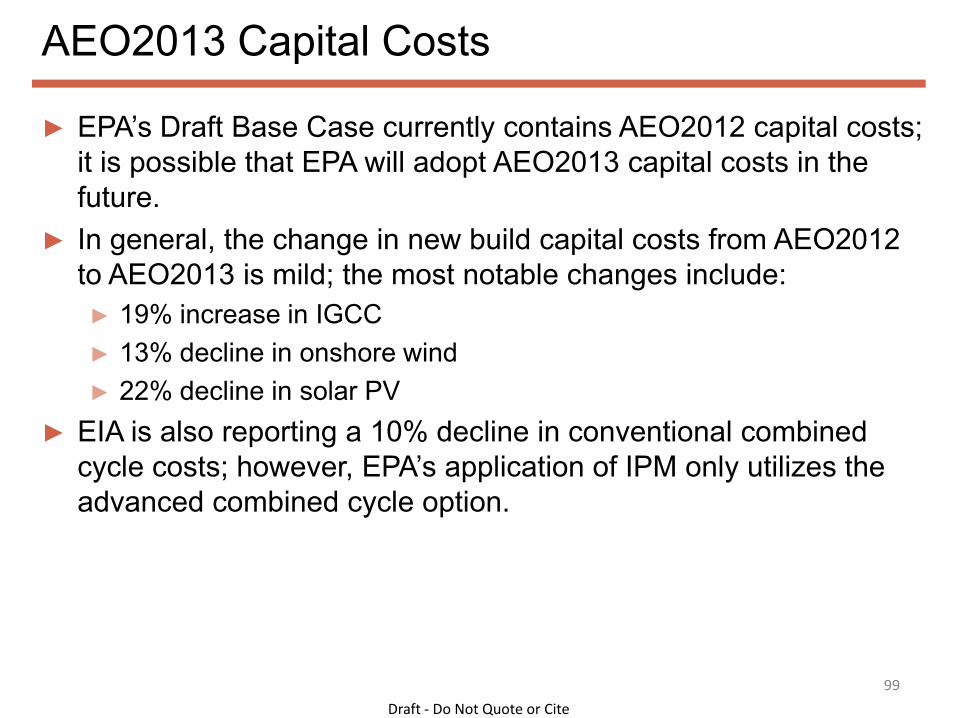
AEO2013 Capital Costs

► EPA’s Draft Base Case currently contains AEO2012 capital costs; it is possible that EPA will adopt AEO2013 capital costs in the future.

► In general, the change in new build capital costs from AEO2012 to AEO2013 is mild; the most notable changes include:

► 19% increase in IGCC ► 13% decline in onshore wind ► 22% decline in solar PV

► EIA is also reporting a 10% decline in conventional combined cycle costs; however, EPA’s application of IPM only utilizes the advanced combined cycle option.

99


Retrofit Cost and Performance

100


Retrofit Option Orientation

► There are two basic types of retrofit controls – reported controls and applied controls.

► Reported controls consist of the retrofit types found in EPA’s summary results:

► Scrubbers – wet and dry ► SCR ► SNCR ► ACI ► CCS ► DSI

► Applied controls are modeled as cost and performance changes that units choose to absorb:

► NOx combustion controls ► Fabric filters ► ESP upgrades ► Scrubber upgrades

► In addition, there are plant modification/modernization costs, such as boiler modifications for fuel switching, life extension costs, and – potentially - heat rate improvements.

101


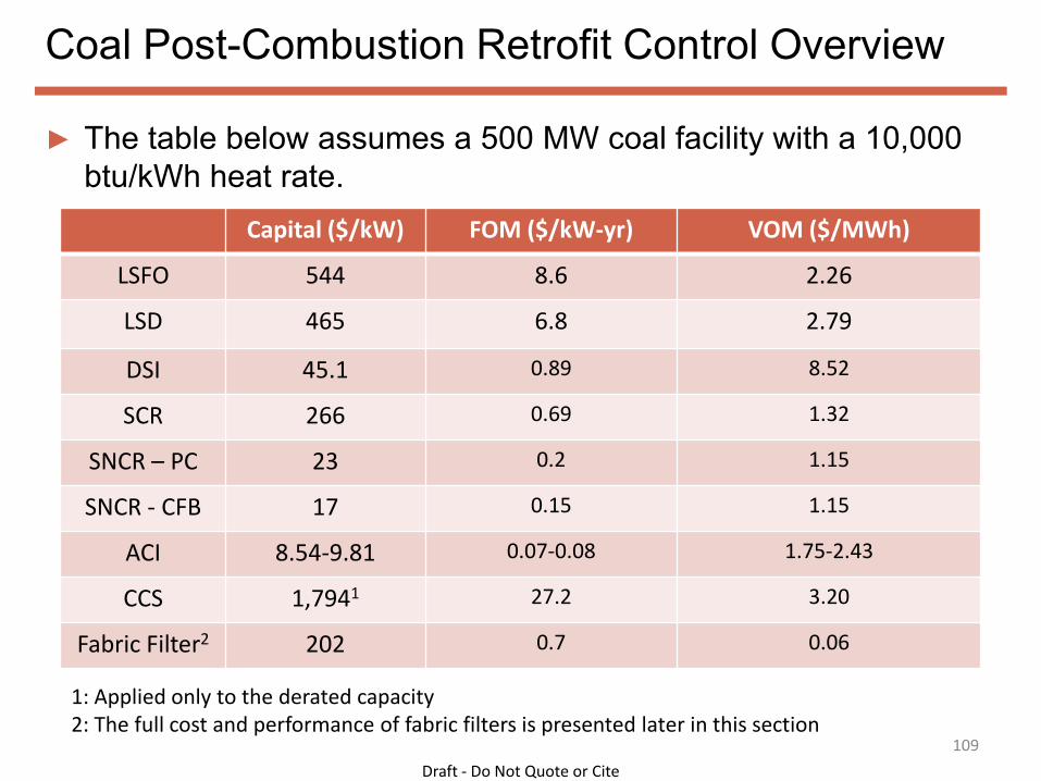
Arriving at a Total Project Cost for New Retrofits

► The total project cost for SO2 and NOx post-combustion controls are built up by cost module:

► Absorber island ► Reagent preparation ► Waste handling (SO2) ► Air heater modification (NOx) ► Balance of plant – primarily electrical and site upgrades

► The total expense of each cost module is impacted by a number of potential factors:

► Unit size ► Heat rate ► Current emission rate ► Coal rank ► Retrofit difficulty

102


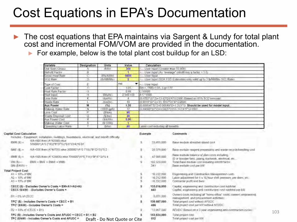
Cost Equations in EPA’s Documentation

103

► The cost equations that EPA maintains via Sargent & Lundy for total plant cost and incremental FOM/VOM are provided in the documentation.

► For example, below is the total plant cost buildup for an LSD:


Capacity and Heat Rate Penalties

► The operation of post-combustion retrofit controls reduces the amount of power available for sale to the grid (i.e. ‘parasitic load’).

► To capture this impact, EPA reduces the generating unit’s capacity by the percentage of generation required to operate the control. This is the capacity penalty associated with the control.

► For example, a wet scrubber installed on a 10,000 btu/kWh heat rate facility results in a capacity penalty of 1. 67%.

► However, the ‘parasitic load’ does not disappear - it still requires fuel consumption. To capture this, a heat rate penalty is imposed that restores fuel consumption to pre-capacity penalty levels.

► The heat rate penalty does not necessarily include a deterioration in the thermal efficiency of the facility resulting from control installation. 104


SO2 Post-Combustion Control Overview

Scrubber Type Heat Rate (Btu/kWh)

100 MW 500 MW 1000 MW Capacity

Penalty (%) Heat Rate

Penalty (%) VOM

(mills/kWh) Capital ($/kW)

FOM ($/kW-yr)

Capital ($/kW)

FOM ($/kW-yr)

Capital ($/kW)

FOM ($/kW-yr)

LSFO 9,000 819 23.7 519 8.3 426 6.4 -1.50 1.53 2.03

10,000 860 24.2 544 8.6 447 6.6 -1.67 1.70 2.26 11,000 899 24.6 569 8.9 467 6.8 -1.84 1.87 2.49

LSD 9,000 701 17.3 444 6.5 422 5.3 -1.18 1.20 2.51

10,000 734 17.7 465 6.8 442 5.5 -1.32 1.33 2.79 11,000 766 18.0 485 7.0 461 5.7 -1.45 1.47 3.07

105

Heat Rate (Btu/kWh)

Dry Sorbent Injection

Capacity Penalty (%)

Heat Rate Penalty (%)

VOM (mills/kWh)

100 MW 500 MW 1000 MW

Capital ($/kW)

FOM ($/kW-yr)

Capital ($/kW)

FOM ($/kW-yr)

Capital ($/kW)

FOM ($/kW-yr)

9,000 138.5 3.71 43.7 0.88 31.6 0.52 -0.64 0.65 7.67

10,000 142.8 3.75 45.1 0.89 35.1 0.55 -0.71 0.72 8.52

11,000 146.8 3.78 46.4 0.90 38.6 0.58 -0.79 0.79 9.38

► For all post-combustion controls, installations for unit sizes smaller than 100 MW receive the costs of a 100 MW unit.


NOx Post-Combustion Control Overview

106

Control Type Heat Rate (Btu/kWh)

100 MW 500 MW 1000 MW Capacity Penalty

(%)

Heat Rate Penalty (%)

VOM (mills/kWh) Capital

($/kW) FOM

($/kW-yr) Capital ($/kW)

FOM ($/kW-yr)

Capital ($/kW)

FOM ($/kW-yr)

SCR

9,000 321 1.76 243 0.64 222 0.53 -0.54 0.54 1.23

10,000 349 1.86 266 0.69 244 0.57 -0.56 0.56 1.32

11,000 377 1.96 289 0.73 265 0.62 -0.58 0.59 1.41

SNCR - Tangential

9,000 55 0.48 22 0.20 15 0.13

-0.05 0.78

1.04

10,000 56 0.50 23 0.20 15 0.14 1.15

11,000 57 0.51 23 0.21 16 0.14 1.27

SNCR - Fluidized Bed

9,000 41 0.36 17 0.15 11 0.10

-0.05 0.78

1.04

10,000 42 0.37 17 0.15 12 0.10 1.15

11,000 43 0.38 17 0.15 12 0.10 1.27


Hg Post-Combustion Control Overview

107

Control Type Heat Rate (Btu/kWh)

100 MW 500 MW 1000 MW Capacity

Penalty (%) Heat Rate

Penalty (%) VOM

(mills/kWh) Capital ($/kW)

FOM ($/kW-yr)

Capital ($/kW)

FOM ($/kW-yr)

Capital ($/kW)

FOM ($/kW-yr)

ACI (Existing ESP)

9,000 37.89 0.32 9.65 0.08 5.35 0.04 -0.10 0.10 2.19

10,000 38.51 0.32 9.81 0.08 5.44 0.05 -0.11 0.11 2.43

11,000 39.07 0.33 9.95 0.08 5.52 0.05 -0.12 0.12 2.68

ACI (Existing FF)

9,000 33.03 0.28 8.41 0.07 4.66 0.04 -0.04 0.04 1.57

10,000 33.54 0.28 8.54 0.07 4.74 0.04 -0.04 0.04 1.75

11,000 34.02 0.29 8.66 0.07 4.81 0.04 -0.05 0.05 1.92


CO2 Post-Combustion Control Overview

Applicability (Original MW Size) 400-750 MW > 750 MW

Capital Cost (2011 $/kW) 1,794 1,707

FOM (2011 $/kW-yr) 27.2 18.8

VOM (2011 (mills/kWh) 3.2 3.2

Capacity Penalty (%) 25% 25%

Heat Rate Penalty (%) 33% 33%

CO2 Removal (%) 90% 90%

108


Coal Post-Combustion Retrofit Control Overview

109

Capital ($/kW) FOM ($/kW-yr) VOM ($/MWh)

LSFO 544 8.6 2.26

LSD 465 6.8 2.79

DSI 45.1 0.89 8.52

SCR 266 0.69 1.32

SNCR – PC 23 0.2 1.15

SNCR - CFB 17 0.15 1.15

ACI 8.54-9.81 0.07-0.08 1.75-2.43

CCS 1,7941 27.2 3.20

Fabric Filter2 202 0.7 0.06

► The table below assumes a 500 MW coal facility with a 10,000 btu/kWh heat rate.

1: Applied only to the derated capacity 2: The full cost and performance of fabric filters is presented later in this section


Coal Post-Combustion Removal Efficiency

Control Type Removal Rate for Target Pollutant Coal Restrictions

LSFO 96% SO2 (0.06 lbs/MMBtu floor)/ 99% HCl All

LSD 92% SO2 (0.065 lbs/MMBtu floor)/ 99% HCl <=3lbs/MMBtu

DSI 70% SO2*/ 90% HCl <=2 lbs/MMBtu

SCR 90% (0.07 lb/MMBtu floor for bituminous; 0.05

lbs/MMBtu for subbituminous ) All

SNCR 25% PC; 50% CFB All

ACI 90% All

CCS 90% All

110

*Recent tests indicate that 90% HCl removal is likely to occur with a lower level of sorbent than initially anticipated. EPA is currently evaluating this assumption.


Applied Controls Overview

► NOx combustion controls are activated if a unit is subject to a policy that controls for NOx emissions

► Assumed technology includes LNB, OFA, etc. ► There are two PM controls in EPA’s Base Case

► ESP upgrades, which are dependent on the difference between historical PM emissions and the MATS standard.

► The installation of a fabric filter is required for some retrofit options; it is also applied as a standalone cost for those units that do not meet the MATS PM standard and do not have an (upgradeable) ESP.

► Below are the costs assumed in EPA’s Draft Base Case for a new fabric filter:

► EPA’s Base Case also contains scrubber upgrades for facilities not currently achieving HCl compliance with an existing scrubber. 111

Heat Rate (Btu/kWh)

Capacity (MW)

Capacity/Heat Rate Penalty (%) VOM (mills/kWh)

100 500 1000

Capital ($/kW)

FOM ($/kW-yr)

Capital ($/kW)

FOM ($/kW-yr)

Capital ($/kW)

FOM ($/kW-yr)

9,000 251 0.9 185 0.6 162 0.6 -0.60 0.05 10,000 274 1.0 202 0.7 177 0.6 -0.60 0.06 11,000 296 1.0 218 0.8 191 0.7 -0.60 0.07


Financial Assumptions

114


Overview of Financial Assumptions

► Investment options are only partially defined by the cost and performance characteristics provided in the previous two sections; financing parameters and costs play an important role.

► Decisions are made in IPM based on minimizing the net present value of capital plus operating costs over the run horizon.

► Two key concepts in the pursuit of this goal are: 1. Capital charge rate – completing the cost picture for investments 2. Discount rate – evaluating decisions and options across various

time periods in the planning horizon

115


Discount Rate

► IPM utilizes the discount rate to evaluate the balance of costs and revenues accruing in different time periods.

► A common manifestation is in cap-and-trade programs, where the allowance price will rise at the discount rate, provided an allowance banking mechanism is available.

► The proposed default discount rate for EPA’s Draft Base Case v.5.13 is 4.77%, consistent with the WACC for a new CC.

► Due to current economic conditions, the risk free rate utilized in v5 to calculate the discount rate is lower than in v4.

► EPA is continuing to evaluate the merits of a lower discount rate based on the implied risk-free rate from 2008-2012.

► The discount rate for a particular capacity type (weighted average cost of capital) plays an important role in the calculation of the capital charge rate.

116


Capital Charge Rate Overview

► The capital charge rate is used to convert a one-time capital expenditure into a stream of levelized annual payments that satisfies the particular investment’s internal rate of return.

► This annual payment can be thought of as equivalent to the project’s required EBITDA, with the capital charge rate representing the ratio of EBITDA to total capital expenditure (capital cost * installed capacity).

► The project incurs this annualized capital cost for the duration of its book life.

► $/kW * CCR = $/kW-yr ► $/kW-yr/Annual Generation = Levelized Capital Cost

117


Capital Charge Rate by Technology Type

118

New Investment Technology Capital Capital Charge Rate

Environmental Retrofits (Utility) 11.51%

Environmental Retrofits (Merchant) 16.18%

Advanced Combined Cycle 10.26%

Advanced Combustion Turbine 10.63%

New Coal (SCPC and Advanced) 12.57%

Advanced Coal with Carbon Capture 9.68%

Nuclear (Without PTC) 9.44%

Nuclear (With PTC) 7.97%

Biomass 9.53%

Wind, Landfill Gas, Solar and Geothermal 10.85%


Financial Updates for Existing Coal Facilities

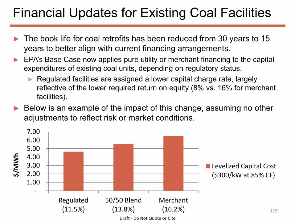
► The book life for coal retrofits has been reduced from 30 years to 15 years to better align with current financing arrangements.

► EPA’s Base Case now applies pure utility or merchant financing to the capital expenditures of existing coal units, depending on regulatory status.

► Regulated facilities are assigned a lower capital charge rate, largely reflective of the lower required return on equity (8% vs. 16% for merchant facilities).

► Below is an example of the impact of this change, assuming no other adjustments to reflect risk or market conditions.

119

- 1.00 2.00 3.00 4.00 5.00 6.00 7.00

Regulated (11.5%)

50/50 Blend (13.8%)

Merchant (16.2%)

$/M

Wh

Levelized Capital Cost ($300/kW at 85% CF)


Questions and Discussion

120


[email protected]


Demand, Transmission, and Resource Adequacy

May 3, 2013 by




Overview: Topics in this Session

► Development of Demand in Draft EPA Base Case v5.13 using IPM

► Demand Regions and Overall US Demand Projections ► Assignment of Demand to Regions and Load Segments

► Treatment of Transmission in Draft EPA Base Case v5.13 using

IPM ► Structure of Interregional Transmission ► Transmission Constraints

► Resource Adequacy

► Regional Reserve Margins ► Resource Adequacy Calculation ► Capacity Avoided Costs


Company Confidential – Do Not Distribute This graphic was obtained from ICF International.

EPA’s Application of IPM®

Demand Regions in Draft EPA Base Case v5.13

► Number of Regions have Increased from Previous Versions ► Total of 75 Model Regions ► US regions increase from 32 to 64 ► Canadian regions unchanged ► Organized around NERC Assessment Areas

► Design benefits ► Better alignment with RTOs/ISOs ► Better treatment of transmission limits and flows ► More closely aligned with dispatch ► Greater demand resolution


US Regions in Draft EPA Base Case v5.13 using IPM


Representing Regional Demand

► IPM Represents Demand by ► IPM region ► Year ► Season (Summer and Winter) ► Load Segment


Developing Regional Demand

► Total US Demand based on AEO Projections ► Each of the 22 AEO/EMM regional demands treated separately ► Demand is Allocated to IPM regions to be consistent with these

regional demands ► Canadian demand based on National Energy Board of Canada study

► Allocating Demand from AEO Regions to IPM Region and Load Segment

► Assign Balancing Areas to 64 IPM regions and 22 NEMS regions ► Use Balancing Areas to calculate each IPM region’s share of each

NEMS region’s load – this creates a mapping from NEMS net energy for load to IPM region.

► Assign NEMS demand to IPM regions using the mapping and net energy for load data from AEO projections

► Assign demand to load segment using hourly data by planning/control area


128

0.00%

5.00%

10.00%

15.00%

20.00%

25.00%

30.00%

35.00%

40.00%

45.00%

50.00%

2016 2020 2025 2030 2040 2050

Change in Annual and Peak Demand (Percent Change from 2016)

Annual Demand (TWh) (All)

Peak demand (MW) (All)


Transmission

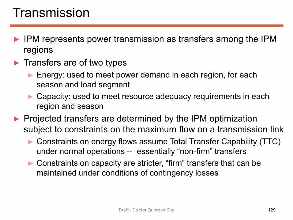
► IPM represents power transmission as transfers among the IPM regions

► Transfers are of two types ► Energy: used to meet power demand in each region, for each

season and load segment ► Capacity: used to meet resource adequacy requirements in each

region and season ► Projected transfers are determined by the IPM optimization

subject to constraints on the maximum flow on a transmission link ► Constraints on energy flows assume Total Transfer Capability (TTC)

under normal operations -- essentially “non-firm” transfers ► Constraints on capacity are stricter, “firm” transfers that can be

maintained under conditions of contingency losses


Transmission

► Transmission constraints in IPM are based on public sources where possible

► These sources include publicly available reports from RTOs and from planning authorities

► Public sources are also verified/supplemented by load flow studies and expert judgement when required

► The maximum potential transfers are also subject to two different

types of limits ► Limits on the quantity that can be transferred between pairs of IPM

regions ► Limits on the total quantity that can be transferred between groups of

regions – these limits are known as “Joint Bounds”


Schematic Example of Transmission Limits and Joint Bounds

► In this example ► Region1 can transfer up to 200 MW

to Region 3 ► Region 2 can transfer up to 300 MW

to Region 3 ► If there were no other limits, Region 1

and 2 could transfer a total of 500 MW to Region 3.

► However, in this example, there is a Joint Bound of 400 MW for combined total transfers from Regions 1 and 2 into Region 3.

► This type of Joint Bound might be used if transfers from Region 2 to Region 3 flowed over the lines between Region 1 and Region 3 (known as “Loop flow”)

131

Region 1

Region 2

Region 3

300 MW

200 MW

400 MW


Costs of Transmission in Draft EPA Base Case v5.13: Losses, Wheeling Charges, and Congestion

► Losses ► Loss percentage of 2.8% on all links between IPM Regions ► Based on EIA State Electricity Profiles 2010 report

► Wheeling Charges ► No charges within IPM regions ► Charges vary depending on region

• No charges imposed between regions within an RTO • Between other regions charges reflect cost of wheeling

► Congestion ► Congestion costs occur when links between regions or joint bounds

among regions are binding and constrain power flows ► Binding constraints cause increased costs by increasing the cost of

generation in the destination region


Limitations of IPM transmission representation in EPA Draft Base Case v5.13

► IPM is not a power flow model ► Does not directly represent real electrical properties of flows in the grid,

such as loop flow or voltage requirements ► Can represent the impact of loop flows using joint bounds where

information is available

► IPM does not directly represent transmission constraints within model regions

► IPM could represent the impact of some of these constraints – such as the need for voltage support – by placing constraints on generation in the model region

• For example, could require some units to run in high load segments for selected run years

► However, specifying such requirements is difficult to justify when using the model for policy impact purposes, and has not been done in the EPA Draft base case

• Would need to be sure requirement would be independent of potential policy scenarios, or be able to provide modeling options to satisfy the requirement


Draft EPA Base Case v5.13 for New York/New England: Sample Results

800

800

1650 1600

1650

2600

1600

2600

3250

1200 1600

1999

1550

1300

2650

175

283

760 760

1999

3450

1600

3500

4350

530

1290

1130

900

1200 1500

1700

1600

150

Transmission Capacities (Energy Flows)

A&B

C&E

D

F

K

G,H,I

J


800

800

1650 1600

1650

2600

1600

2600

3250

1200 1600

1999

1550

1300

2650

175

283

760 760

1999

3450

1600

3500

4350

530

1290

1130

900

1200 1500

1700

1600

150

Energy Flows in Summer Segment 1

(Peak 36 Hours)

1689

1500

1700

513

3450

150

922

1489

760 561

4350

322

1650

A&B

C&E

D

F

K

G,H,I

J

Joint Bound Limits and Flows Path Limit Flow %

ISO NE to NYISO 1,730 1,082 62.6% NY (K to G,H,I,J) 285 37 12.9% NY (G,H,I,J to K) 1,465 561 38.3% NYISO to ISO NE 1,730 150 8.7%

37




800

800

1650 1600

1650

2600

1600

2600

3250

1200 1600

1999

1550

1300

2650

175

283

760 760

1999

3450

1600

3500

4350

530

1290

1130

900

1200 1500

1700

1600

150


(Next 147 Hours)

1821

1500

1700

1827

3450

1085

2444

760 943

4350

900

1650

A&B

C&E

D

F

K

G,H,I

J


ISO NE to NYISO 1,730 1,673 96.7% NY (K to G,H,I,J) 285 112 39.3% NY (G,H,I,J to K) 1,465 943 64.3% NYISO to ISO NE 1,730 0 0.0%

481

112

13



800

800

1650 1600

1650

2600

1600

2600

3250

1200 1600

1999

1550

1300

2650

175

283

760 760

1999

3450

1600

3500

4350

530

1290

1130

900

1200 1500

1700

1600

150


(Next 367 Hours)

1649

1500

1700

2281

3450

1160

1804

760 1173

4350

800

1650

A&B

C&E

D

F

K

G,H,I

J


ISO NE to NYISO 1,730 1,560 90.2% NY (K to G,H,I,J) 285 285 100.0% NY (G,H,I,J to K) 1,465 1,173 80.1% NYISO to ISO NE 1,730 0 0.0%

283

1283



800

800

1650 1600

1650

2600

1600

2600

3250

1200 1600

1999

1550

1300

2650

175

283

760 760

1999

3450

1600

3500

4350

530

1290

1130

900

1200 1500

1700

1600

150


(Next 1102 Hours)

1655

1500

1700

2216

3450

908

1104

760 1290

4350

766

1650

1171

1461

A&B

C&E

D

F

K

G,H,I

J


ISO NE to NYISO 1,730 1,526 88.2% NY (K to G,H,I,J) 285 0 0.0% NY (G,H,I,J to K) 1,465 1,290 88.1% NYISO to ISO NE 1,730 0 0.0%



800

800

1650 1600

1650

2600

1600

2600

3250

1200 1600

1999

1550

1300

2650

175

283

760 760

1999

3450

1600

3500

4350

530

1290

1130

900

1200 1500

1700

1600

150


(Next 1102 Hours)

1453

1500

1700

1956

3161

566

13 1290

4350

1650

A&B

C&E

D

F

K

G,H,I

J


ISO NE to NYISO 1,730 12 0.7% NY (K to G,H,I,J) 285 0 0.0% NY (G,H,I,J to K) 1,465 1,465 100.0% NYISO to ISO NE 1,730 0 0.0%

175

1176



800

800

1650 1600

1650

2600

1600

2600

3250

1200 1600

1999

1550

1300

2650

175

283

760 760

1999

3450

1600

3500

4350

530

1290

1130

900

1200 1500

1700

1600

150


(Lowest 918 Hours)

742

1532

1334

121

505

698

2418

A&B

C&E

D

F

K

G,H,I

J


ISO NE to NYISO 1,730 0 0.0% NY (K to G,H,I,J) 285 0 0.0% NY (G,H,I ,J to K) 1,465 1,094 74.7% NYISO to ISO NE 1,730 0 0.0%

792


Resource Adequacy

► Resource adequacy in the EPA Base Case v5.13 is based on a target reserve margin in each region.

► Generally, target reserve margins are based on the margin in the NERC assessments, unless there are more specific requirements at the state level

► Each IPM region must maintain sufficient reserve margin capacity to cover peak load plus the target margin in each season

► Capacity may be internal to the region or transferred from other regions

► Capacity from other regions is subject to losses and to limits on capacity transfers

► Reserve margin capacity is 100% of a unit’s capacity except for wind, solar and hydro.


Resource Adequacy and Capacity

► Resource Adequacy Drives the Value of Capacity ► In IPM the avoided cost of capacity in each model region and season

depends on: • The peak demand (summer and winter) • The capacity resources in the region • The available capacity in other regions • The costs and constraints of importing capacity • The required reserve margins

► The expected value of capacity is a key component of the decision to build new plants in IPM:

► Reserve margins decrease over the planning horizon, as • Demand grows • Plants retire, and • IPM builds new plants to ensure adequate margin.




143

Thank You

Date post:	10-Apr-2018
Category:	Documents
Upload:	doanhuong
View:	216 times
Download:	2 times

EPA’s Power Sector - EEI€¦ · · 2013-06-20EPA’s Power Sector Modeling Workshop 1 Focus,...

Documents