EPI Distortion Correction - mrdac.uni- · PDF fileEPI Distortion Correction Works-in-Progress...

EPI Distortion Correction

Works-in-Progress package Version 2.6

For SIEMENS Magnetom

Sonata/Avanto/Espree/TRIO/7T

Installation and User’s Guide NUMARIS/4 VA25, VB11, VB12, VB13, VB15

Maxim Zaitsev, PhD

March 31, 2008

Magnetic Resonance Development and Application Center

MRDAC - Freiburg, University Hospital Freiburg, Germany

Contact: Hugstetterstr. 55, D 79106 Freiburg, email: [email protected], phone: +49 761 270-7412, fax -7413

Page 2 Magnetom Sonata/Avanto/Espree/TRIO/7T, Numaris/4 VA25 VB11 VB12 VB13 VB15

Table of Contents

1 General Remarks................................................................................................4 1.1 Preface..........................................................................................................4 1.2 Disclaimer .....................................................................................................4 1.3 Revision History ............................................................................................4

2 Method principles and implementation ............................................................5 2.1 Point Spread Function Mapping Technique ..................................................5 2.2 Implementation..............................................................................................7 2.3 Diffusion Package Option............................................................................11 2.4 7T Notes......................................................................................................13 2.5 References..................................................................................................14

3 Software Installation Procedure......................................................................15 3.1 Automatic Installation ..................................................................................15 3.2 Manual Installation, pre VB13 (BOLD-only).................................................15 3.3 Manual Installation, pre VB13 (Full Package) .............................................17 3.4 Manual Installation, VB13/VB15 (BOLD only) .............................................19 3.5 Manual Installation, VB13 (Full Package)....................................................20 3.6 Post-Installation Steps for DW-EPI..............................................................21

4 Sequences and Protocols................................................................................23 4.1 General Remarks ........................................................................................23 4.2 What’s New in Version 2.5 ..........................................................................23 4.3 What’s New in Version 2.5.1 .......................................................................23 4.4 What’s New in Version 2.6 ..........................................................................23 4.5 Common new functionality ..........................................................................23

4.5.1 7T Relevant Features...........................................................................24 4.5.2 Detailed description of the common extensions...................................24

4.6 New Parameters, PSF mapping..................................................................26 4.7 New Parameters, EPI..................................................................................27 4.8 New Parameters, DW-EPI...........................................................................28 4.9 Note on EVA Protocols................................................................................30 4.10 EVA Protocol Parameters for PSF Reconstruction......................................31 4.11 EVA Protocol Parameters for Application of Corrections.............................31 4.12 Remarks on Reconstruction Performance...................................................32

5 Workflow ...........................................................................................................34 5.1 General Remarks ........................................................................................34 5.2 Performing Distortion Correction Online......................................................34


5.3 Issues Specific to the Diffusion-Weighted EPI ............................................34 5.4 Retrospective Reconstruction of the PSF or EPI data.................................35 5.5 Performing Distortion Correction Offline......................................................36


1 General Remarks 1.1 Preface This package being a substantial commitment from our side is provided free of charge for everybody to benefit. In order to encourage the continued development of the package feel free to reference the following paper(s) in you publications:

M. Zaitsev, J. Hennig and O. Speck. PSF Mapping with Parallel Imaging Techniques with High Accelerations Factors: Fast, Robust and Flexible Method for EPI Distortion Correction. Magn Reson Med 2004; 52:1156-66.

1.2 Disclaimer The software and the associated documentation (the “Software”) is provided “as is”, without warranty of any kind, express or implied, including but not limited to the warranties of merchantability, fitness for a particular purpose and noninfringement. In no event shall the authors or copyright holders be liable for any claim, damages or other liability, whether in an action of contract, tort or otherwise, arising from, out of or in connection with the Software or the use or other dealings in the Software. 1.3 Revision History V 1.0 23.10.2003 Original release. V 2.0 20.01.2005 New release with extended functionality. V 2.1 07.02.2005 Service release containing no new features. V 2.1.1 20.12.2005 Service release containing only few new features. V 2.5 31.03.2006 New release with numerous improvements. V 2.5.1 23.07.2007 Reimplementation of the package for VB13. V 2.6 07.03.2008 Merge with the 7T version, reimplementation for VB15


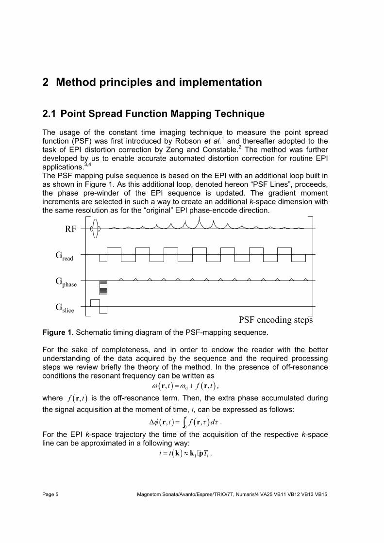
2 Method principles and implementation 2.1 Point Spread Function Mapping Technique The usage of the constant time imaging technique to measure the point spread function (PSF) was first introduced by Robson et al.1 and thereafter adopted to the task of EPI distortion correction by Zeng and Constable.2 The method was further developed by us to enable accurate automated distortion correction for routine EPI applications.3,4 The PSF mapping pulse sequence is based on the EPI with an additional loop built in as shown in Figure 1. As this additional loop, denoted hereon “PSF Lines”, proceeds, the phase pre-winder of the EPI sequence is updated. The gradient moment increments are selected in such a way to create an additional k-space dimension with the same resolution as for the “original” EPI phase-encode direction.

RF

Gread

Gphase

Gslice

PSF encoding steps

Figure 1. Schematic timing diagram of the PSF-mapping sequence. For the sake of completeness, and in order to endow the reader with the better understanding of the data acquired by the sequence and the required processing steps we review briefly the theory of the method. In the presence of off-resonance conditions the resonant frequency can be written as

( ) ( )0, ,t f tω ω= +r r ,

where ( ),f tr is the off-resonance term. Then, the extra phase accumulated during the signal acquisition at the moment of time, t, can be expressed as follows:

( ) ( )0

, ,t

t f dφ τ τΔ = ∫r r .

For the EPI k-space trajectory the time of the acquisition of the respective k-space line can be approximated in a following way:

( ) 1 lt t T= ≈k k p ,


where p is the unity vector for phase-encode direction and lT is the period time, required to acquire one line in k-space (often referred to as the “echo spacing”). Using the above notation, it is possible to write the standard EPI signal equation in the presence of off-resonance effects:

( ) ( ) ( )( )1

0exp ,lT

VS i f d dρ τ τ⎛ ⎞= ⋅ +⎜ ⎟

⎝ ⎠∫ ∫k p

k r k r r r .

The integral under the exponential expresses the undesired space-varying phase accumulation, which is causing EPI image distortions. The signal delivered by the PSF-mapping sequence is convenient to describe in terms of two wave vectors:

( ) ( ) ( ) ( )1

1 2 0,

1 2,T

i f diS e e dτ τ

ρ + ⋅ ∫= ∫k p

rk k rk k r r ,

where 1k corresponds to the EPI trajectory, whilst 2k describes the most conventional gradient-echo (GE) encoding. The Fourier transform of the above equation with respect to both 1k and 2k yields the following image intensity:

( ) ( ) ( ) ( ) ( )121 2 1 01 1 2 2

,

1 2 1 2 1 2 2 1, ,T

i f dii iI S e e d d e e dτ τ

ρ ⋅ −− ⋅ − ⋅ ∫= =∫∫ ∫k p

rk r rk r k rr r k k k k r k . As seen, the reconstructed image is a result of multiplication of the proton density in undistorted coordinates, ( )2ρ r , with a term, which we will refer to as space-varying

point-spread function, ( )1 2,H r r :

( ) ( ) ( )121 2 1 0

,

1 2 1,T

i f diH e e dτ τ⋅ − ∫= ∫

k prk r rr r k .

For the case of stationary off-resonance effects, when ( ) ( )0,f fτ ≈r r , the above equation transforms to:

( ) ( )( )1 2 2 1 0 2,H fδ= − +r r r r p r , which is more familiar form of the point spread function in presence of the off-resonance conditions. It is important to note, that the integration of the PSF image intensity, ( )1 2,I r r , along the distorted dimension, 1r , yields the undistorted GE image:

( ) ( ) ( )

( ) ( ) ( )

( )

121 2 1 0

1 2 1 2 1 2 1

,

2 1 1

2

, ,T

i f di

I d H d

e e d dτ τ

ρ

ρ

ρ

⋅ −

=

∫=

=

∫ ∫

∫ ∫k p

rk r r

r r r r r r r

r k r

r

.

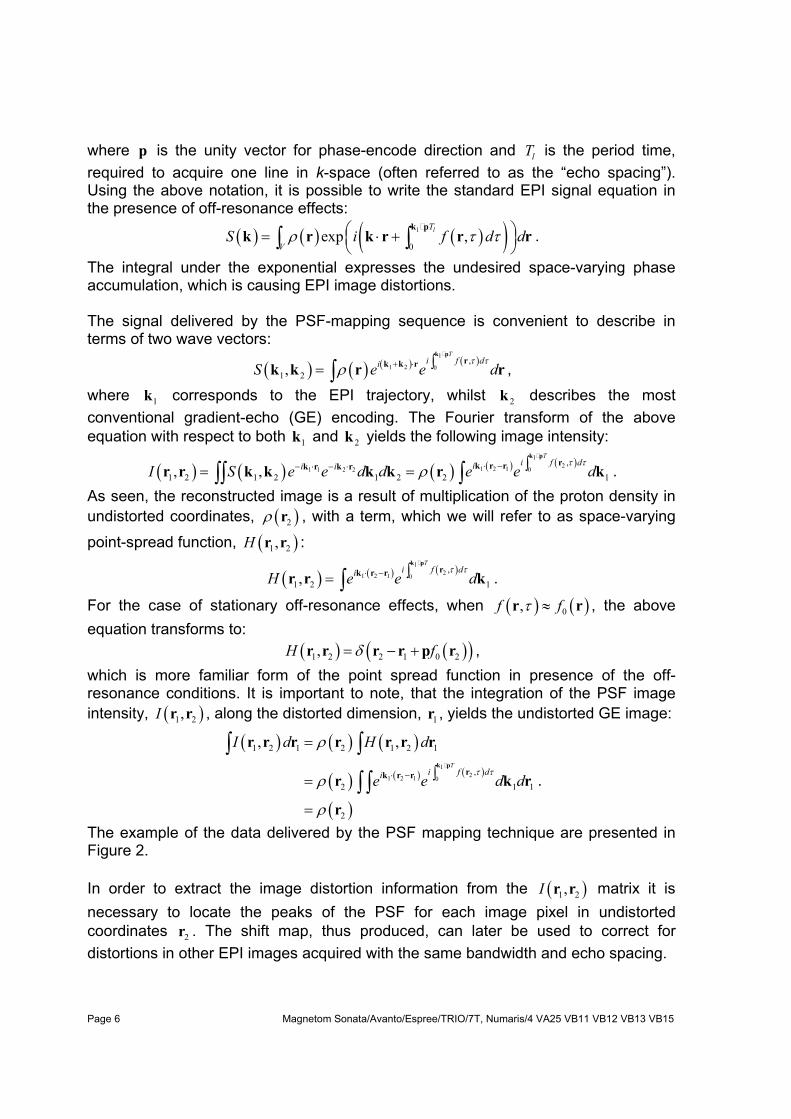
The example of the data delivered by the PSF mapping technique are presented in Figure 2. In order to extract the image distortion information from the ( )1 2,I r r matrix it is necessary to locate the peaks of the PSF for each image pixel in undistorted coordinates 2r . The shift map, thus produced, can later be used to correct for distortions in other EPI images acquired with the same bandwidth and echo spacing.


(a) (b) (c) Figure 2. Data delivered by the PSF mapping technique: distorted EPI image (a), undistorted GE image (b) and example of the PSF view in Y1-Y2 coordinates(c).

2.2 Implementation1 The PSF mapping package is implemented as a set of the following program modules:

• PSF mapping sequence, • ICE program for PSF reconstruction (a functor library in VB13) • Optional ICE program for online diffusion reconstruction • Four (optionally six) EVA functors for completing the PSF reconstruction and

applying the corrections and the • EPI sequence with minor modifications • Optional DW-EPI sequence with free diffusion encoding.

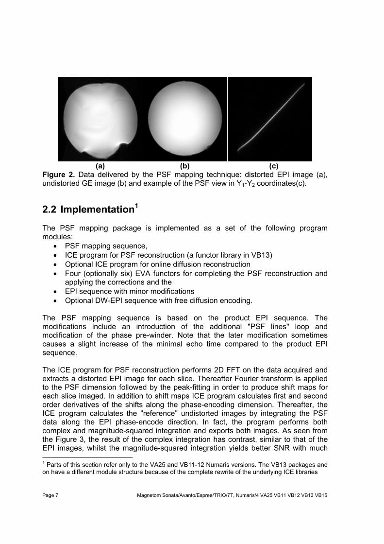
The PSF mapping sequence is based on the product EPI sequence. The modifications include an introduction of the additional "PSF lines" loop and modification of the phase pre-winder. Note that the later modification sometimes causes a slight increase of the minimal echo time compared to the product EPI sequence. The ICE program for PSF reconstruction performs 2D FFT on the data acquired and extracts a distorted EPI image for each slice. Thereafter Fourier transform is applied to the PSF dimension followed by the peak-fitting in order to produce shift maps for each slice imaged. In addition to shift maps ICE program calculates first and second order derivatives of the shifts along the phase-encoding dimension. Thereafter, the ICE program calculates the "reference" undistorted images by integrating the PSF data along the EPI phase-encode direction. In fact, the program performs both complex and magnitude-squared integration and exports both images. As seen from the Figure 3, the result of the complex integration has contrast, similar to that of the EPI images, whilst the magnitude-squared integration yields better SNR with much 1 Parts of this section refer only to the VA25 and VB11-12 Numaris versions. The VB13 packages and on have a different module structure because of the complete rewrite of the underlying ICE libraries


flatter contrast. This makes the later image a good source for the subsequently required tissue segmentation. The ICE program thus produces 6 image sets, which are stored in the image database on the host. The images for shift and shift derivative may appear rather strange because of the high noise in the areas of low signal. This is, however, rather normal.

a) b)

Figure 3. Result of the complex (a) and magnitude-squared (b) integration. Note lower contrast and higher SNR in the second image.

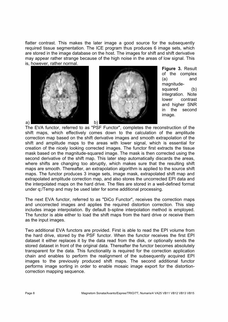
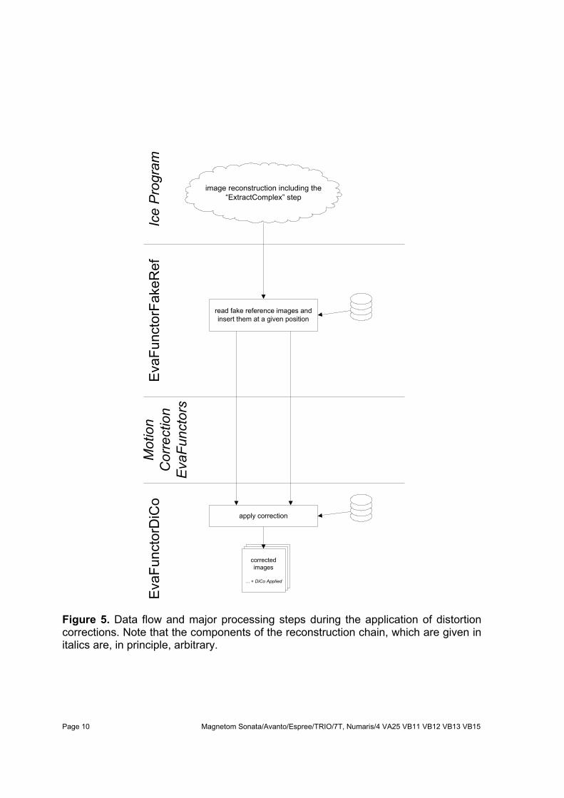
The EVA functor, referred to as "PSF Functor", completes the reconstruction of the shift maps, which effectively comes down to the calculation of the amplitude correction map based on the shift derivative images and smooth extrapolation of the shift and amplitude maps to the areas with lower signal, which is essential for creation of the nicely looking corrected images. The functor first extracts the tissue mask based on the magnitude-squared image. The mask is then corrected using the second derivative of the shift map. This later step automatically discards the areas, where shifts are changing too abruptly, which makes sure that the resulting shift maps are smooth. Thereafter, an extrapolation algorithm is applied to the source shift maps. The functor produces 3 image sets, image mask, extrapolated shift map and extrapolated amplitude correction map, and also stores the uncorrected EPI data and the interpolated maps on the hard drive. The files are stored in a well-defined format under q:/Temp and may be used later for some additional processing. The next EVA functor, referred to as "DiCo Functor", receives the correction maps and uncorrected images and applies the required distortion correction. This step includes image interpolation. By default b-spline interpolation method is employed. The functor is able either to load the shift maps from the hard drive or receive them as the input images. Two additional EVA functors are provided. First is able to read the EPI volume from the hard drive, stored by the PSF functor. When the functor receives the first EPI dataset it either replaces it by the data read from the disk, or optionally sends the stored dataset in front of the original data. Thereafter the functor becomes absolutely transparent for the data. This functionality is required for the correction application chain and enables to perform the realignment of the subsequently acquired EPI images to the previously produced shift maps. The second additional functor performs image sorting in order to enable mosaic image export for the distortion-correction mapping sequence.


Raw Data

3D-FT, unwrapping, integration, filtering, maximum interpolation

uncorrectedimages

DiCo Uncorrected

‘raw’ distortionmaps

DiCo Internal(Raw Shifts)

reference std. dev.Images

DiCo Internal(Reference HQ)

referenceimages

DiCo Reference

thresholding

segmentedmask

DiCo SegmentationMask

apply mask, inter/extra-polate, filter

processeddistortion

maps

DiCo ProcessedShifts

apply correction

correctedimages

… + DiCo Applied

Psf

IceF

unct

orP

sfE

vaFu

ncto

rE

vaFu

ncto

rDiC

o

secondderivative of

the ‘raw’distortion map

DiCo Internal(Raw Shifts Deriv2)

first derivativeof the ‘raw’

distortion mapDiCo Internal

(Raw Shifts Deriv)

processedamplitudecorrection

mapsDiCo Processed

Amplitude

Figure 4. Data flow and major processing steps during the PSF mapping reconstruction. Image-sorting functor is not shown for the sake of readability


read fake reference images andinsert them at a given position

apply correction

correctedimages

… + DiCo Applied

Ice

Pro

gram

Eva

Func

torF

akeR

efE

vaFu

ncto

rDiC

o

image reconstruction including the“ExtractComplex” step

Mot

ion

Cor

rect

ion

Eva

Func

tors

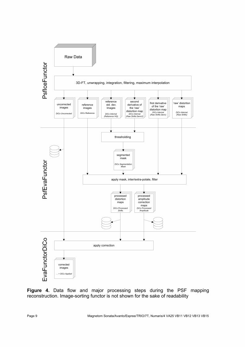
Figure 5. Data flow and major processing steps during the application of distortion corrections. Note that the components of the reconstruction chain, which are given in italics are, in principle, arbitrary.


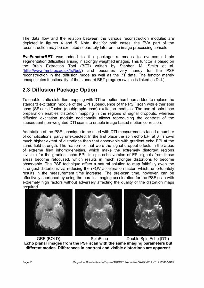
The data flow and the relation between the various reconstruction modules are depicted in figures 4 and 5. Note, that for both cases, the EVA part of the reconstruction may be executed separately later on the image processing console. EvaFunctorBET was added to the package a means to overcome brain segmentation difficulties arising in strongly weighted images. This functor is based on the Brain Extraction Tool (BET) written by Stephen M. Smith et al. (http://www.fmrib.ox.ac.uk/fsl/bet/) and becomes very handy for the PSF reconstruction in the diffusion mode as well as the 7T data. The functor merely encapsulates functionality of the standard BET program (which is linked as DLL). 2.3 Diffusion Package Option To enable static distortion mapping with DTI an option has been added to replace the standard excitation module of the EPI subsequence of the PSF scan with either spin echo (SE) or diffusion (double spin-echo) excitation modules. The use of spin-echo preparation enables distortion mapping in the regions of signal dropouts, whereas diffusion excitation module additionally allows reproducing the contrast of the subsequent non-weighted DTI scans to enable image based motion correction. Adaptation of the PSF technique to be used with DTI measurements faced a number of complications, partly unexpected. In the first place the spin echo EPI at 3T shown much higher extent of distortions than that observable with gradient echo EPI at the same field strength. The reason for that were the signal dropout effects in the areas of extreme filed inhomogeneities, which make the extremely distorted regions invisible for the gradient echo EPI. In spin-echo version of EPI signals from those areas become refocused, which results in much stronger distortions to become observable. The PSF technique offers a natural solution to map faithfully even the strongest distortions via reducing the rFOV acceleration factor, which, unfortunately results in the measurement time increase. The pre-scan time, however, can be effectively shortened by using the parallel imaging acceleration for the PSF scan with extremely high factors without adversely affecting the quality of the distortion maps acquired.

GRE (BOLD) SpinEcho Double Spin Echo (DTI) Echo planar images from the PSF scan with the same imaging parameters but different modes. Differences in contrast and visible distortions are apparent.


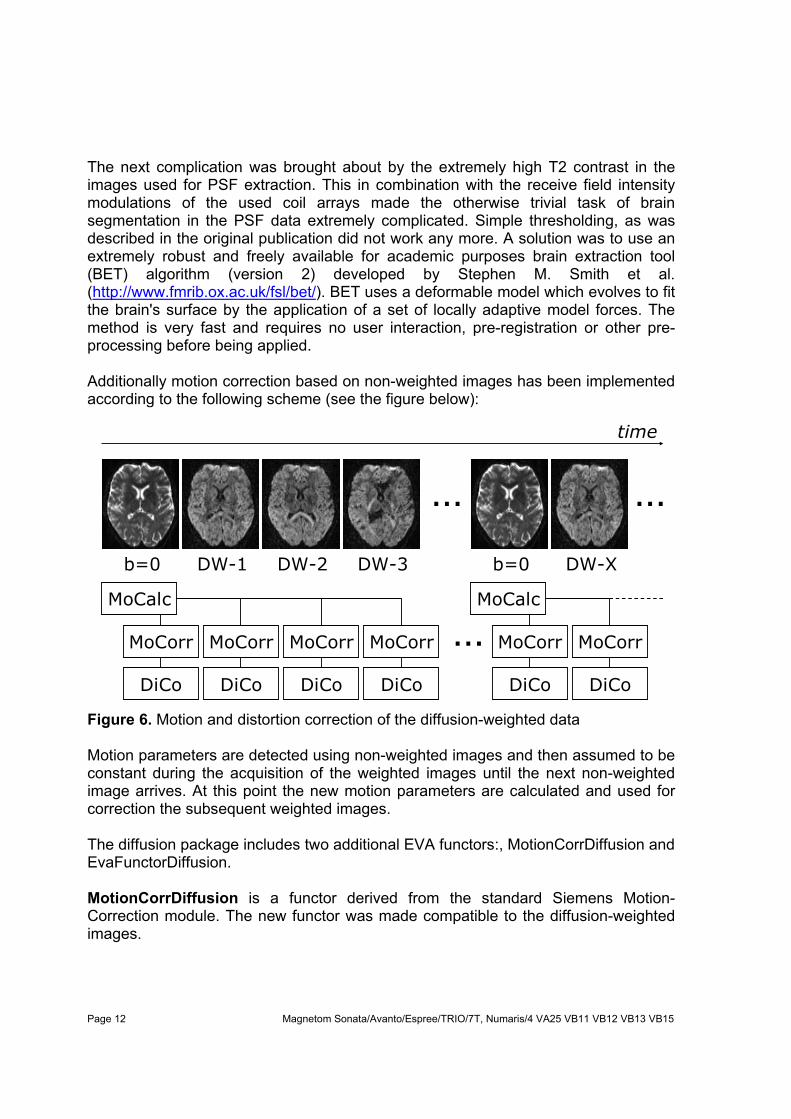
The next complication was brought about by the extremely high T2 contrast in the images used for PSF extraction. This in combination with the receive field intensity modulations of the used coil arrays made the otherwise trivial task of brain segmentation in the PSF data extremely complicated. Simple thresholding, as was described in the original publication did not work any more. A solution was to use an extremely robust and freely available for academic purposes brain extraction tool (BET) algorithm (version 2) developed by Stephen M. Smith et al. (http://www.fmrib.ox.ac.uk/fsl/bet/). BET uses a deformable model which evolves to fit the brain's surface by the application of a set of locally adaptive model forces. The method is very fast and requires no user interaction, pre-registration or other pre-processing before being applied. Additionally motion correction based on non-weighted images has been implemented according to the following scheme (see the figure below):

MoCorr

DiCo

b=0

…

DW-1 DW-2 DW-3

…

b=0 DW-X

time

MoCalc

MoCorr

DiCo

MoCorr MoCorr …DiCo DiCo

MoCalc

MoCorr

DiCo

MoCorr

DiCo

Figure 6. Motion and distortion correction of the diffusion-weighted data Motion parameters are detected using non-weighted images and then assumed to be constant during the acquisition of the weighted images until the next non-weighted image arrives. At this point the new motion parameters are calculated and used for correction the subsequent weighted images. The diffusion package includes two additional EVA functors:, MotionCorrDiffusion and EvaFunctorDiffusion. MotionCorrDiffusion is a functor derived from the standard Siemens Motion-Correction module. The new functor was made compatible to the diffusion-weighted images.


EvaFunctorDiffusion2 implements magnitude-domain averaging and the standard diffusion calculation routines, as in the product diffusion ice program. That is the trace and ADC calculation is not possible with MDDW data. 2.4 7T Notes Imaging at 7 Tesla is not a trivial task, especially when EPI sequence needs to be used. On the other hand, echo planar images acquired at 7T without distortion correction are nearly unusable. The PSF distortion mapping package works at 7T, however, one shall be much more careful at choosing parameters and controlling the results. As one of the most critical parts of the PSF reconstruction, we most strongly recommend to check whether the “DiCo Segmentation Mask” really fits the measured object (typically brain). Here are some hints how to achieve the best results at 7 Tesla and above.

• Use sinusoidal readout to lower helium boil-off and acoustic noise • Lower Fat-Sat flip angle and bandwidth-time-product of the excitation pulse to

save SAR • Use parallel imaging acceleration of 2 or 3 with EPI to reduce distortions and

the echo time • PSF “images” are much more strongly T2-weighted, which complicates

thresholding a lot. Optimize simple cut of threshold for your imaging parameters, then switch on BET and be prepared to optimize its parameters as well.

• When using an array coil severe signal dropouts may be observed in the PSF “Reference” images. Use “Late combination” to work around this issue.

7 Tesla option is a very recent addition, that is why do not be surprised if something works not as smooth as you might get used to at 3T. At this juncture we are very interested to receive your feedback and ideas for improvements.

2 EvaFunctorDiffusion is only a part of pre-VB13 packets


2.5 References

1. Robson MD, Gore JG, Constable RT. Measurement of the Point Spread Function in MRI Using Constant Time Imaging. Magn Reson Med 1997;38:733-740

2. Zeng H, Constable RT. Image Distortion Correction in EPI: Comparison of Field Mapping With Point Spread Function Mapping. Magn Reson Med 2002;48:137-146

3. Zaitsev M, Hennig J, Speck O. Automated Online EPI Distortion Correction for fMRI Applications. Proc Intl Soc Mag Reson Med, Toronto, 2003; p.1042

4. Zaitsev M, Hennig J, Speck O. PSF Mapping with Parallel Imaging Techniques with High Accelerations Factors: Fast, Robust and Flexible Method for EPI Distortion Correction. Magn Reson Med 2004; 52:1156-66.

5. Speck O, Stadler J, Zaitsev M. High resolution single-shot EPI at 7T. MAGMA in press, due to appear in spring of 2008


3 Software Installation Procedure An installation script, install.bat, is provided to automate the installation procedure. In case automatic installation fails, it is possible to proceed with manual installation, as described below. 3.1 Automatic Installation Automatic installation of on the scanner includes the following steps: Start SDE shell or command shell (CMD). Change into the directory, where the package archive was unpacked. Start the installation script by typing:

install.bat Make sure that the script completed successfully without error or warning messages. Create the new default protocols:

Open the Exam Explorer, select a protocol location, select ‘Insert … Sequence’, select ‘Folder: USER’, select ‘mz_epi2d_psf’, click ‘Insert’. Double click the new protocol and adjust the parameters as desired. Open the Exam Explorer, select a protocol location, select ‘Insert … Sequence’, select ‘Folder: USER’, select ‘mz_epi2d_bold_dc’, click ‘Insert’. Double click the new protocol and adjust the parameters as desired. Make sure the parameters for the EPI protocol are completely identical to those of the respective PSF mapping protocol. In case you have the full package: Open the Exam Explorer, select a protocol location, select ‘Insert … Sequence’, select ‘Folder: USER’, select ‘mz_epi2d_diff_free’, click ‘Insert’. Double click the new protocol and adjust the parameters as desired. Make sure the parameters for the DW-EPI protocol are identical where possible to those of the respective PSF mapping protocol. Very important for VB13/VB15: Go to the “PostProc” card and deactivate DtiIcePostProcFunctor option.

In case you have the full package be sure to complete the “Post-Installation Steps for DW-EPI” described below. 3.2 Manual Installation, pre VB13 (BOLD-only) Manual installation of on the scanner includes the following steps:


Start SDE shell or command shell (CMD). Change into the directory, where the package archive was unpacked. Copy the PSF sequence file for the host to the customer sequence directory:

copy mz_ep2d_psf.dll %CustomerSeq% . Check, which MPCU model your scanner equipped with. Depending on that copy the correct PSF sequence file for the MPCU to the corresponding sequence directory by execution one of the following commands:

copy mz_ep2d_psf.m603 %CustomerSeq% copy mz_ep2d_psf.m750 %CustomerSeq% copy mz_ep2d_psf.ia86 %CustomerSeq%

Copy the EPI sequence file for the host to the customer sequence directory:

copy mz_ep2d_bold_dc.dll %CustomerSeq% Check, which MPCU model your scanner equipped with. Depending on that copy the correct EPI sequence file for the MPCU to the corresponding sequence directory by execution one of the following commands:

copy mz_ep2d_bold_dc.m603 %CustomerSeq% copy mz_ep2d_bold_dc.m750 %CustomerSeq% copy mz_ep2d_bold_dc.ia86 %CustomerSeq%

Copy the ICE program to the customer ICE directory:

copy mz_IceProgramPSF.dll %CustomerIceProgs% Copy the EVA program to the customer EVA directory:

copy mz_EvaFunctorPSF.dll q:\bin Copy the additional dynamic library to the ICE computer:

copy newPAT.dll q:\bin Copy the default EVA protocols to the customer default EVA protocol directory:

mkdir %CustomerEvaDefProt%\DistCorr copy MrEvaPSF.evp %CustomerEvaDefProt%\DistCorr copy MrEvaApplyMoCoDiCo.evp %CustomerEvaDefProt%\DistCorr

Create the new default protocols:

Open the Exam Explorer, select a protocol location, select ‘Insert … Sequence’, select ‘Folder: USER’, select ‘mz_epi2d_psf’, click ‘Insert’. Double click the new protocol and adjust the parameters as desired. Open the Exam Explorer, select a protocol location, select ‘Insert … Sequence’, select ‘Folder: USER’, select ‘mz_epi2d_bold_dc’, click ‘Insert’. Double click the new protocol and adjust the parameters as desired. Make


sure the parameters for the EPI protocol are completely identical to that of the respective PSF mapping protocol.

Optionally you may install the offline post-processing part:

Copy the EVA program to the offline EVA directory:

copy mz_EvaFunctorPSF.dll %MEDHOME%\bin Copy the EVA protocols to the offline EVA protocol directory:

copy MrEvaPSF.evp %MEDHOME%\IDEA\EvaProt copy MrEvaApplyMoCoDiCo.evp %MEDHOME%\IDEA\EvaProt

3.3 Manual Installation, pre VB13 (Full Package) Manual installation of on the scanner includes the following steps: Start SDE shell or command shell (CMD). Change into the directory, where the package archive was unpacked. Copy the PSF sequence file for the host to the customer sequence directory:

copy mz_ep2d_psf.dll %CustomerSeq% . Check, which MPCU model your scanner equipped with. Depending on that copy the correct PSF sequence file for the MPCU to the corresponding sequence directory by execution one of the following commands:

copy mz_ep2d_psf.m603 %CustomerSeq% copy mz_ep2d_psf.m750 %CustomerSeq% copy mz_ep2d_psf.ia86 %CustomerSeq%

Copy the EPI sequence file for the host to the customer sequence directory:

copy mz_ep2d_bold_dc.dll %CustomerSeq% Check, which MPCU model your scanner equipped with. Depending on that copy the correct EPI sequence file for the MPCU to the corresponding sequence directory by execution one of the following commands:

copy mz_ep2d_bold_dc.m603 %CustomerSeq% copy mz_ep2d_bold_dc.m750 %CustomerSeq% copy mz_ep2d_bold_dc.ia86 %CustomerSeq%

Copy the ICE programs to the customer ICE directory:

copy mz_IceProgramPSF.dll %CustomerIceProgs% copy mz_IceProgramOnlineDiff2D.dll %CustomerIceProgs%

Copy the EVA program to the customer EVA directory:


copy mz_EvaFunctorPSF.dll q:\bin copy mz_EvaFunctorBET.dll q:\bin copy mz_EvaFunctorDiffusion.dll q:\bin

Copy the additional dynamic libraries to the ICE computer:

copy newPAT.dll q:\bin copy bet2dll.dll q:\bin

Copy the default EVA protocols to the customer default EVA protocol directory:

mkdir %CustomerEvaDefProt%\DistCorr copy MrEvaPSF.evp %CustomerEvaDefProt%\DistCorr copy MrEvaApplyMoCoDiCo.evp %CustomerEvaDefProt%\DistCorr mkdir %CustomerEvaDefProt%\Diffusion copy DiffMoCoDiCoMosaic.evp %CustomerEvaDefProt%\Diffusion

Copy the diffusion direction table to the C:\Medcom\Temp:

copy DTI_Directions.dat c:\medcom\temp Create the new default protocols:

Open the Exam Explorer, select a protocol location, select ‘Insert … Sequence’, select ‘Folder: USER’, select ‘mz_epi2d_psf’, click ‘Insert’. Double click the new protocol and adjust the parameters as desired. Open the Exam Explorer, select a protocol location, select ‘Insert … Sequence’, select ‘Folder: USER’, select ‘mz_epi2d_bold_dc’, click ‘Insert’. Double click the new protocol and adjust the parameters as desired. Make sure the parameters for the EPI protocol are completely identical to those of the respective PSF mapping protocol. Open the Exam Explorer, select a protocol location, select ‘Insert … Sequence’, select ‘Folder: USER’, select ‘mz_epi2d_diff_free’, click ‘Insert’. Double click the new protocol and adjust the parameters as desired. Make sure the parameters for the DW-EPI protocol are identical where possible to those of the respective PSF mapping protocol.

Optionally you may install the offline post-processing part:

Copy the EVA program to the offline EVA directory:

copy mz_EvaFunctorPSF.dll %MEDHOME%\bin Copy the EVA protocols to the offline EVA protocol directory:

copy MrEvaPSF.evp %MEDHOME%\IDEA\EvaProt copy MrEvaApplyMoCoDiCo.evp %MEDHOME%\IDEA\EvaProt

Be sure to complete the “Post-Installation Steps for DW-EPI” described below.


3.4 Manual Installation, VB13/VB15 (BOLD only) Manual installation of on the scanner includes the following steps: Start Windows command shell (CMD). Change into the directory, where the package archive was unpacked. Copy the PSF sequence files for the host to the customer sequence directory:

copy mz_ep2d_psf.dll %CustomerSeq% copy mz_ep2d_psf.i86 %CustomerSeq%

Copy the EPI sequence files for the host to the customer sequence directory:

copy mz_ep2d_bold_dc.dll %CustomerSeq% copy mz_ep2d_bold_dc.i86 %CustomerSeq%

Copy the win32 ICE modules and typelibs to the appropriate directory:

copy bet2dll.dll %MedHome%\bin copy IceSineEPI.dll %MedHome%\bin copy IceSineEPI.evp %MedHome%\bin copy mz_EvaFunctorBET.dll %MedHome%\bin copy mz_EvaFunctorBET.evp %MedHome%\bin copy mz_PsfEvaFunctors.dll %MedHome%\bin copy mz_PsfEvaFunctors.evp %MedHome%\bin copy mz_PsfIceFunctors.dll %MedHome%\bin copy mz_PsfIceFunctors.evp %MedHome%\bin

Copy the xlinux64 ICE modules and typelibs to the appropriate directory:

copy libIceSineEPI.so %MRIRHOME%\lib copy libmz_EvaFunctorBET.so %MRIRHOME%\lib copy libmz_PsfEvaFunctors.so %MRIRHOME%\lib copy libmz_PsfIceFunctors.so %MRIRHOME%\lib

Copy the ICE “programs” to the customer ICE directory:

copy mz_IceProgram2D_Sine.evp %CustomerIceProgs% copy mz_IceProgramPSF.evp %CustomerIceProgs% copy mz_IceProgramPSF_Sine.evp %CustomerIceProgs%


mkdir %CustomerEvaDefProt%\DistCorr copy MrEvaPSF.evp %CustomerEvaDefProt%\DistCorr copy MrEvaApplyMoCoDiCo.evp %CustomerEvaDefProt%\DistCorr

Create the new default protocols:


Open the Exam Explorer, select a protocol location, select ‘Insert … Sequence’, select ‘Folder: USER’, select ‘mz_epi2d_psf’, click ‘Insert’. Double click the new protocol and adjust the parameters as desired. Open the Exam Explorer, select a protocol location, select ‘Insert … Sequence’, select ‘Folder: USER’, select ‘mz_epi2d_bold_dc’, click ‘Insert’. Double click the new protocol and adjust the parameters as desired. Make sure the parameters for the EPI protocol are completely identical to those of the respective PSF mapping protocol.

3.5 Manual Installation, VB13 (Full Package) Manual installation of on the scanner includes the following steps: Start Windows command shell (CMD). Change into the directory, where the package archive was unpacked. Copy the PSF sequence files for the host to the customer sequence directory:

copy mz_ep2d_psf.dll %CustomerSeq% copy mz_ep2d_psf.i86 %CustomerSeq%

Copy the EPI sequence files for the host to the customer sequence directory:

copy mz_ep2d_bold_dc.dll %CustomerSeq% copy mz_ep2d_bold_dc.i86 %CustomerSeq%

Copy the DTI sequence files for the host to the customer sequence directory:

copy mz_ep2d_diff_free.dll %CustomerSeq% copy mz_ep2d_diff_free.i86 %CustomerSeq%

Copy the win32 ICE modules and typelibs to the appropriate directory:

copy bet2dll.dll %MedHome%\bin copy IceSineEPI.dll %MedHome%\bin copy IceSineEPI.evp %MedHome%\bin copy mz_EvaFunctorBET.dll %MedHome%\bin copy mz_EvaFunctorBET.evp %MedHome%\bin copy mz_PsfEvaFunctors.dll %MedHome%\bin copy mz_PsfEvaFunctors.evp %MedHome%\bin copy mz_PsfIceFunctors.dll %MedHome%\bin copy mz_PsfIceFunctors.evp %MedHome%\bin copy mz_DiffusionFunctors.dll %MedHome%\bin copy mz_DiffusionFunctors.evp %MedHome%\bin

Copy the xlinux64 ICE modules and typelibs to the appropriate directory:

copy libIceSineEPI.so %MRIRHOME%\lib copy libmz_EvaFunctorBET.so %MRIRHOME%\lib


copy libmz_PsfEvaFunctors.so %MRIRHOME%\lib copy libmz_PsfIceFunctors.so %MRIRHOME%\lib copy libmz_DiffusionFunctors %MRIRHOME%\lib

Copy the ICE “programs” to the customer ICE directory:

copy mz_IceProgram2D_Sine.evp %CustomerIceProgs% copy mz_IceProgramDiffusion2D.evp %CustomerIceProgs% copy mz_IceProgramDiffusion2D_Sine.evp %CustomerIceProgs% copy mz_IceProgramPSF.evp %CustomerIceProgs% copy mz_IceProgramPSF_Sine.evp %CustomerIceProgs%


mkdir %CustomerEvaDefProt%\DistCorr copy MrEvaPSF.evp %CustomerEvaDefProt%\DistCorr copy MrEvaApplyMoCoDiCo.evp %CustomerEvaDefProt%\DistCorr mkdir %CustomerEvaDefProt%\DTI copy DtiMoCoDiCoMosaic.evp %CustomerEvaDefProt%\DTI

Copy the diffusion direction table to the C:\Medcom\Temp:

copy DTI_Directions.dat c:\medcom\temp Create the new default protocols:

Open the Exam Explorer, select a protocol location, select ‘Insert … Sequence’, select ‘Folder: USER’, select ‘mz_epi2d_psf’, click ‘Insert’. Double click the new protocol and adjust the parameters as desired. Open the Exam Explorer, select a protocol location, select ‘Insert … Sequence’, select ‘Folder: USER’, select ‘mz_epi2d_bold_dc’, click ‘Insert’. Double click the new protocol and adjust the parameters as desired. Make sure the parameters for the EPI protocol are completely identical to those of the respective PSF mapping protocol. Open the Exam Explorer, select a protocol location, select ‘Insert … Sequence’, select ‘Folder: USER’, select ‘mz_epi2d_diff_free’, click ‘Insert’. Double click the new protocol and adjust the parameters as desired. Make sure the parameters for the DW-EPI protocol are identical where possible to those of the respective PSF mapping protocol. Very important: Go to the “PostProc” card and deactivate DtiIcePostProcFunctor option.

Be sure to complete the “Post-Installation Steps for DW-EPI” described below. 3.6 Post-Installation Steps for DW-EPI3 Because of the unclear file access permission configuration issues on Numaris VB the file “DTI_Directions.dat” located in “c:\medcom\temp” cannot be read by the 3 Only relevant for Numaris VB11, VB12 and VB13. VB15 seems not to suffer from this problem.


diffusion sequence during its execution. This leads to the failure of the sequence to start. To complete the installation of the diffusion sequence:

1. Create any valid protocol based on the mz_ep2d_diff_free sequence 2. Start the sequence (it will not succeed) 3. Open “c:\medcom\temp” in explorer, make sure you are able to find the file

“DTI_Directions.dat” 4. Open “DTI_Directions.dat” it in the text editor 5. Locate file called

“PLEASE_PASTE_CONTENTS_OF__DTI_directions.dat__HERE_AND_RENAME_THE_FILE”, open it in the text editor and paste content of “DTI_Directions.dat” into it

6. Close text editors 7. Delete “DTI_Directions.dat” 8. Rename “PLEASE_...” into “DTI_Directions.dat”


4 Sequences and Protocols 4.1 General Remarks Since the sequences are derived from the standard EPI sequence, the vast majority of the user interface and features are identical to those of this standard EPI. Prior to the first run of the PSF mapping sequence, the standard 3D shim procedure is performed to ensure best field homogeneity. As with the standard EPI this option cannot be disabled. It is important to ensure that no shim alternation occurs later on during the EPI runs, because that would invalidate the distortion maps. As with the standard EPI, due to the high switching rates used, the peripheral nerve stimulation monitor may sometimes not allow the measurement to be performed with the parameters selected. In general, a lower bandwidth will decrease the stimulation and a different selection of the readout gradient may also help (read direction along L/R-axis shows generally the lowest stimulation). 4.2 What’s New in Version 2.5

• VA25/VB11/VB12 support • Free imaging matrix • Inversion recovery preparation with shuffle mode • Spin Echo and Diffusion modes • GRAPPA acceleration for the PSF dimension • Further memory usage optimisation • More accurate and stable masking • EVA parameters are now adjustable by users

4.3 What’s New in Version 2.5.1

• VB13 support 4.4 What’s New in Version 2.6

• VB15 support • 7T relevant features

4.5 Common new functionality All sequences included in the package are based on the EPI template with somewhat extended functionality. This includes thin slice support, slice-selective inversion in “shuffle” mode and flexible matrix size or field of view adjustment possibilities. Although primary motivated by 7T developments, the features in the following section


have also became the common part of the package. Be sure to read the following section even if you are not planning to use the package at 7T. 4.5.1 7T Relevant Features Several new parameters have been added to address the common problems at 7T:

• Specific Adsorption Rate (SAR) control: “FatSat Flip angle”, “Sinc BW time Product” and “Elongate RF-Pulse”

• High Helium boil-off: “Sinusoidal Readout” • Long frequency adjustment: “Repeated Frequency Adjust”

These parameters, amongst the others, are described in detail below. 4.5.2 Detailed description of the common extensions

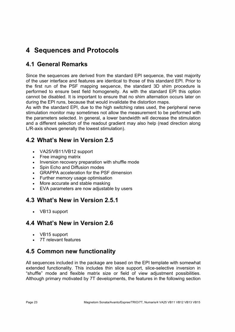
contrast card resolution card

Magnetization preparation: In all sequences “Slice-sel. IR” option is enabled. In contrast to the product sequence the inversion time TI defaults to “0”, which causes the solve handler to be activated once the inversion recovery is selected. This forces the initial TI to be as short as possible. Known bug: under some conditions the standard solve handler fails to adjust both TI and TR. In this case it makes sense to temporarily increase TR prior to activating the inversion recovery. Enable Inversion Shuffle: This new option enables application of the inversion pulses to slices different from the currently acquired one. This enables relatively flexible selection of TI without acquisition time penalty. Known bug: because of the tight link between TI and TR in shuffle mode it is not possible to adjust TR freely. In order to change TR it might be required to temporarily set TI to its minimum. FatSat Flip angle: Allows to reduce the fat saturation flip angle. The default of 110° gives the most dominant contribution to SAR at 7T. As T2* of fat at 7T is very short it is safe to reduce this value down to 30°. FoV Phase: It is now possible to select FoV in phase encoding direction to be larger than that in readout direction. The increments of the FoV in phase encoding direction correspond now to a single k-space line. Known problems: sometimes the sequence might not allow to change some other parameters while non-rectangular FoV is selected. In this case it is advisable to temporarily set FoV phase to 100%.


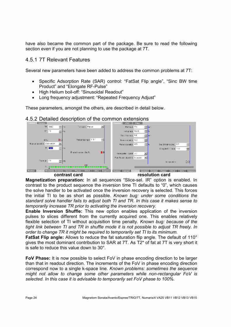
Slice Thickness: In versions prior to 2.6 for slices thinner than 2 mm the duration of the excitation RF pulse is doubled, which enables slice thickness to go down to 1 mm. Starting from 2.6 the duration of the RF pulse is controlled manually using “Elongate RF-Pulse” parameter. Known problem: under some unclear conditions (seemingly depending on TE) the displayed slice thickness is rounded to integer of mm. That is for 1.5 mm slices 2 mm will be displayed. This situation can be detected via disappearing the tens of mm from the display (2 mm is wrong, 2.0 is correct). It helps is this case to vary TR and TE, close and re-open protocol, etc. until the tens of mm reappear. Base Resolution: In contrast to product EPI base resolution of all sequences included in the package is free to choose. Although we did not observe any performance problems when using matrixes not equal to powers of 2, the user must be warned than using these matrixes implies higher computation overhead during the image reconstruction. Known problem: sometimes it is not possible to select some parameters while using non power of 2 matrixes. In this case it is advisable to temporarily change the matrix size. Partial Fourier Algorithm: An experimental feature allowing to activate an advanced partial Fourier reconstruction (POCS). Unfortunately, Siemens implementation of POCS seems to be inferior to the standard zero-filling. Sinc BW time Product: Allows the end user to trade slice profile fidelity for SAR. The default value of 5.2 reproduces the product sequence behavior. Elongate RF-Pulse: (attention, logic change for thin slice support) This parameter is an elongation factor, which allows to control manually the duration of the RF pulse(s) in the sequence. On one hand it may serve to reduce SAR, on the other hand to achieve a higher slice resolution (thinner slices).

system/adjustments card sequence/part1 card

Repeated Frequency Adjust: This flag allows to deactivate the default behavior of repeating frequency adjust on every sequence start. The default value reproduces the product sequence behavior. Readout Type: It is possible now to switch between the standard “Trapezoidal” and “Sinusoidal” readout profiles. The later one serves to the considerable reduction of Helium boil-off on certain 7T systems as well as the sound pressure level on most of the scanners.


Asymmetric echo, Echo Asymmetry factor: These two experimental options allow for asymmetric echoes in read-our direction. At this point it is not clear, whether they can be of an advantage in any way. 4.6 New Parameters, PSF mapping

sequence-special card additional “PSF&DiCo” card

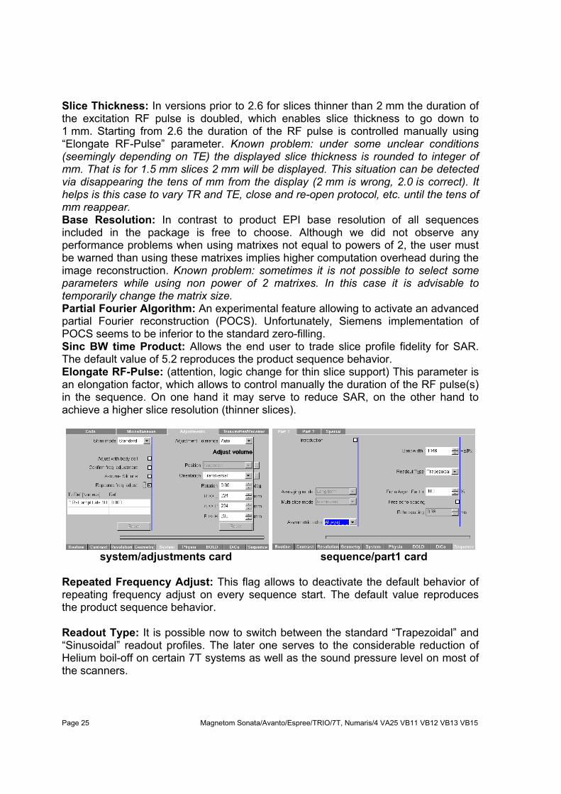
PSF rFOV Factor: Defines the FOV reduction in the PSF-encode direction. Reducing the field of view enables considerable time-saving, but limits the maximal distortions, which can be correctly mapped. Thus for head imaging at 3T machines it is valid to assume that the distortions are smaller that 1/8-th of the FOV, which yields the rFOV factor of 4. At other field strength or for different regions it might be needed to update this parameter respectively. PSF Lines to Measure & PSF Image Lines: These two are read-only parameters, provided for user information. The first one defines the actual number of PSF-encode lines acquired and the second defines the extents of the PSF dimension after the Fourier transform. PSF Hanning Filter: Enables filtering in PSF dimension. Depending on the sequence parameters and the object being imaged, the PSF reconstruction may sometimes produce step-like shift maps. This artifact almost exclusively appears in phantom imaging and can be diminished by enabling the filter option and adjusting the filter width. PSF Filter Width: Sets the strength of the filter in PSF direction. Bigger numbers mean stronger filtering. Please, note that whenever the filtering is at all needed, it must be rather strong (the filter width parameter must be between 64 and 128). PSF Wait for Recon: Holds the sequence from completing until the reconstruction is completed. This option makes sure that no further measurement is performed before the distortion correction maps are ready. PSF Late Combination:4 Forces the use sum-of-squares combination for the reference data. Affects segmentation results for some multi-channel coils. Related to the “Threshold” parameter from the “PSF&DiCo” card, which might need adaptation upon change of the combination mode. PSF Mode: Switches between different magnetization preparation modes for the PSF reference scan. Possible values are "Grad. Echo", "Spin Echo" and "Diffusion". 4 Not available in the VB13 version of the package, present but nit guaranteed to run in VB15


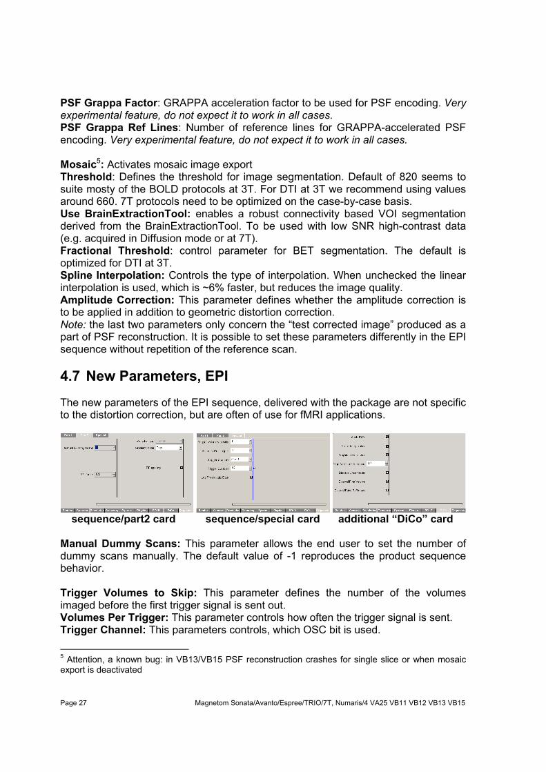
PSF Grappa Factor: GRAPPA acceleration factor to be used for PSF encoding. Very experimental feature, do not expect it to work in all cases. PSF Grappa Ref Lines: Number of reference lines for GRAPPA-accelerated PSF encoding. Very experimental feature, do not expect it to work in all cases. Mosaic5: Activates mosaic image export Threshold: Defines the threshold for image segmentation. Default of 820 seems to suite mosty of the BOLD protocols at 3T. For DTI at 3T we recommend using values around 660. 7T protocols need to be optimized on the case-by-case basis. Use BrainExtractionTool: enables a robust connectivity based VOI segmentation derived from the BrainExtractionTool. To be used with low SNR high-contrast data (e.g. acquired in Diffusion mode or at 7T). Fractional Threshold: control parameter for BET segmentation. The default is optimized for DTI at 3T. Spline Interpolation: Controls the type of interpolation. When unchecked the linear interpolation is used, which is ~6% faster, but reduces the image quality. Amplitude Correction: This parameter defines whether the amplitude correction is to be applied in addition to geometric distortion correction. Note: the last two parameters only concern the “test corrected image” produced as a part of PSF reconstruction. It is possible to set these parameters differently in the EPI sequence without repetition of the reference scan. 4.7 New Parameters, EPI The new parameters of the EPI sequence, delivered with the package are not specific to the distortion correction, but are often of use for fMRI applications.

sequence/part2 card sequence/special card additional “DiCo” card Manual Dummy Scans: This parameter allows the end user to set the number of dummy scans manually. The default value of -1 reproduces the product sequence behavior. Trigger Volumes to Skip: This parameter defines the number of the volumes imaged before the first trigger signal is sent out. Volumes Per Trigger: This parameter controls how often the trigger signal is sent. Trigger Channel: This parameters controls, which OSC bit is used.

5 Attention, a known bug: in VB13/VB15 PSF reconstruction crashes for single slice or when mosaic export is deactivated


Trigger Duration: This parameter sets the duration of the trigger signal. Log Physiologic Data: Enables logging of the physiologic monitoring data, such as EKG, pulse oxymetre and respiration. The log files are created in the directory C:\MedCom\log and are named PmuSignals_XXX.*, where XXX are the sequentially incremented numbers. Apply DiCo: This parameter activates distortion correction routines. Spline Interpolation: Controls the type of interpolation. When unchecked the linear interpolation is used, which is ~6% faster, but reduces the image quality. Amplitude Correction: This parameter defines, whether the amplitude correction is to be applied in addition to geometric distortion correction. Amp. Norm. Lower Bound: This parameters allows to set the lower bound for the global amplitude renormalization upon application of amplitude correction. This possibility shall serve as a means to address the earlier reported problem of the corrected images having extremely low pixel amplitudes. Discard Uncorrected: This parameter defines whether the uncorrected images need not to be stored in the image database. Discard First Volume: This parameter defines whether the first original EPI volume shall be discarded. This option was introduced mainly because of the performance problems during online motion correction (see below). Discard Fake Ref Image: This parameter defines whether the fake reference image (acquired by the PSF scan and stored on disk) needs to be stored in the image database. Default is ‘false’ because of the historical reasons and performance limitations. Note: it is not possible to select at the same time both “Discard First Volume” and “Discard Fake Ref Image”. 4.8 New Parameters, DW-EPI The diffusion-weighted sequence provided with the package in addition to distortion and motion correction amongst the other features (see common functionality above) contains the tree important improvements:

1. Support for arbitrary number of DTI weighting directions 2. Support for flexible number of non-weighted scans 3. Physiologic data logging 4. Online reconstruction allows for literally unlimited data volumes

(VB13/VB15 have no limits on the data volumes) 5. Flexible averaging support via combination of “Averages” and “Repetitions”

(not functional in VB13/VB15)


sequence-special card additional “PostProc” card, preVB13

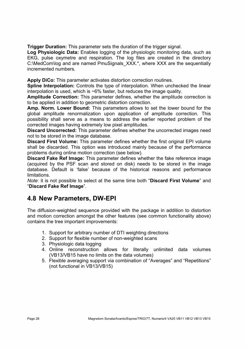
“PostProc” card, VB13/VB15. DtiIcePostProcFunctor must be off.

Log Physiologic Data: Enables logging of the physiologic monitoring data, such as EKG, pulse oxymetre and respiration. The log files are created in the directory C:\MedCom\log and are named PmuSignals_XXX.*, where XXX are the sequentially incremented numbers. Unweighted Scan Period: Controls how often the non-weighted scan (b=0) shall be performed. The tool tip of this parameter reports the total number of non-weighted scans for the current diffusion weighting scheme. Force Slice Coordinates: Forces the diffusion weighting scheme to use slice coordinates instead of the physical coordinates of the gradient system. Apply DiCo: This parameter activates distortion correction routines. Spline Interpolation: Controls the type of interpolation. When unchecked the linear interpolation is used, which is ~6% faster, but reduces the image quality. Amplitude Correction: This parameter defines, whether the amplitude correction is to be applied in addition to geometric distortion correction. Defaults to “false” for diffusion because of the dynamic range considerations. Discard Uncorrected: This parameter defines whether the uncorrected images need not to be stored in the image database. Discard First Volume: This parameter defines whether the first original EPI volume shall be discarded. Discard Fake Ref Image: This parameter defines whether the fake reference image (acquired by the PSF scan and stored on disk) needs to be stored in the image database. Note: it is not possible to select both “Discard First Volume” and “Discard Fake Ref Image”.


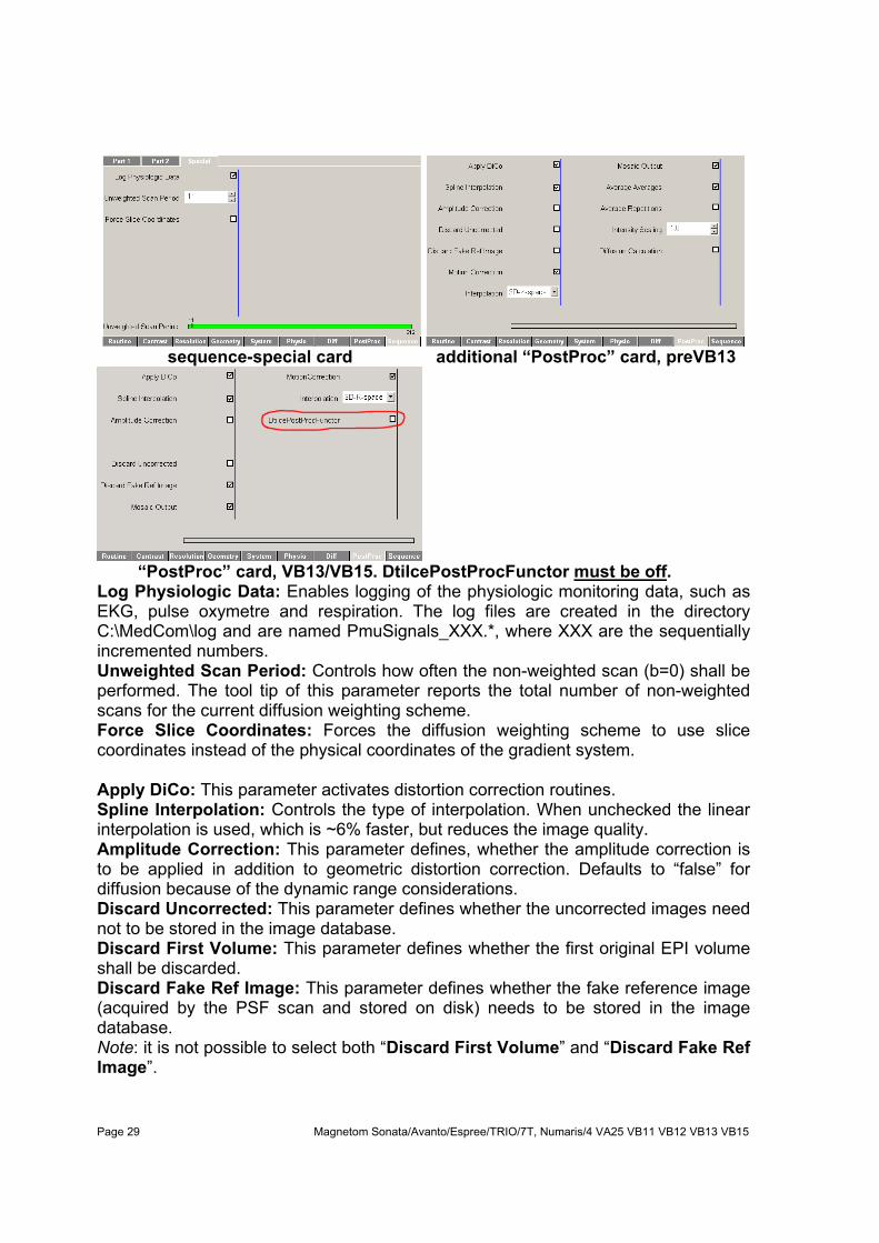
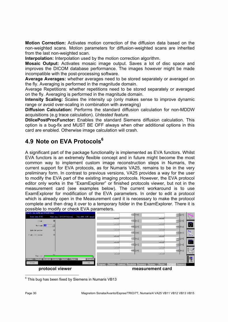
Motion Correction: Activates motion correction of the diffusion data based on the non-weighted scans. Motion parameters for diffusion-weighted scans are inherited from the last non-weighted scan. Interpolation: Interpolation used by the motion correction algorithm. Mosaic Output: Activates mosaic image output. Saves a lot of disc space and improves the DICOM database performance. The images however might be made incompatible with the post-processing software. Average Averages: whether averages need to be stored separately or averaged on the fly. Averaging is performed in the magnitude domain. Average Repetitions: whether repetitions need to be stored separately or averaged on the fly. Averaging is performed in the magnitude domain. Intensity Scaling: Scales the intensity up (only makes sense to improve dynamic range or avoid over-scaling in combination with averaging) Diffusion Calculation: Performs the standard diffusion calculation for non-MDDW acquisitions (e.g trace calculation). Untested feature. DtiIcePostProcFunctor: Enables the standard Siemens diffusion calculation. This option is a bug-fix and MUST BE OFF always when other additional options in this card are enabled. Otherwise image calculation will crash. 4.9 Note on EVA Protocols6 A significant part of the package functionality is implemented as EVA functors. Whilst EVA functors is an extremely flexible concept and in future might become the most common way to implement custom image reconstruction steps in Numaris, the current support for EVA protocols, as for Numaris VA25, remains to be in the very preliminary form. In contrast to previous versions, VA25 provides a way for the user to modify the EVA part of the existing imaging protocols. However, the EVA protocol editor only works in the “ExamExplorer” or finished protocols viewer, but not in the measurement card (see examples below). The current workaround is to use ExamExplorer for modification of the EVA parameters. In order to edit a protocol which is already open in the Measurement card it is necessary to make the protocol complete and then drag it over to a temporary folder in the ExamExplorer. There it is possible to modify or check EVA parameters.

protocol viewer measurement card

6 This bug has been fixed by Siemens in Numaris VB13


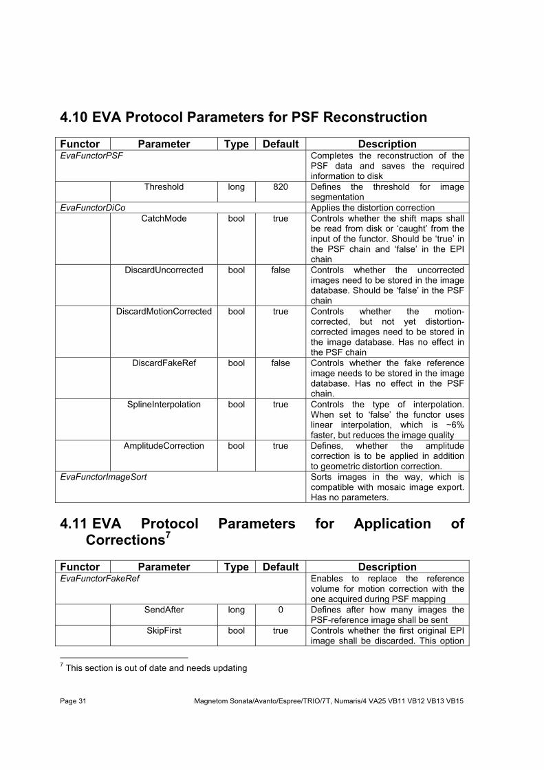
4.10 EVA Protocol Parameters for PSF Reconstruction Functor Parameter Type Default Description EvaFunctorPSF Completes the reconstruction of the

PSF data and saves the required information to disk

Threshold long 820 Defines the threshold for image segmentation

EvaFunctorDiCo Applies the distortion correction CatchMode bool true Controls whether the shift maps shall

be read from disk or ‘caught’ from the input of the functor. Should be ‘true’ in the PSF chain and ‘false’ in the EPI chain

DiscardUncorrected bool false Controls whether the uncorrected images need to be stored in the image database. Should be ‘false’ in the PSF chain

DiscardMotionCorrected bool true Controls whether the motion-corrected, but not yet distortion-corrected images need to be stored in the image database. Has no effect in the PSF chain

DiscardFakeRef bool false Controls whether the fake reference image needs to be stored in the image database. Has no effect in the PSF chain.

SplineInterpolation bool true Controls the type of interpolation. When set to ‘false’ the functor uses linear interpolation, which is ~6% faster, but reduces the image quality

AmplitudeCorrection bool true Defines, whether the amplitude correction is to be applied in addition to geometric distortion correction.

EvaFunctorImageSort Sorts images in the way, which is compatible with mosaic image export. Has no parameters.

4.11 EVA Protocol Parameters for Application of

Corrections7 Functor Parameter Type Default Description EvaFunctorFakeRef Enables to replace the reference

volume for motion correction with the one acquired during PSF mapping

SendAfter long 0 Defines after how many images the PSF-reference image shall be sent

SkipFirst bool true Controls whether the first original EPI image shall be discarded. This option

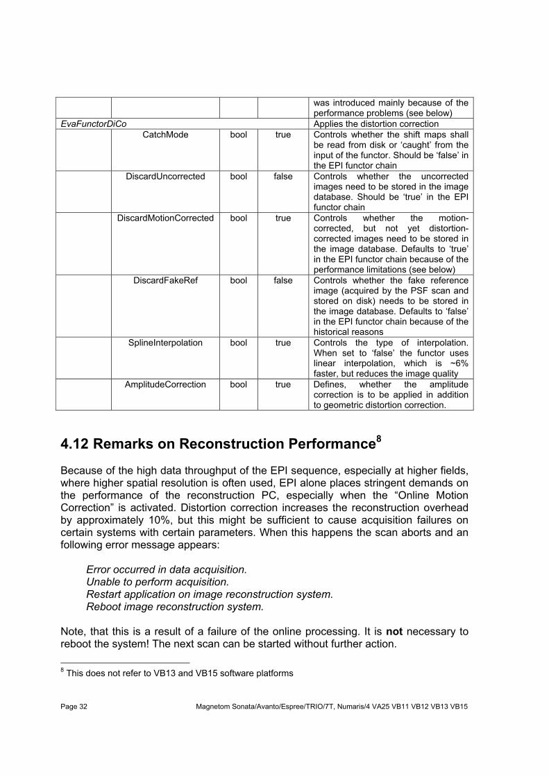
7 This section is out of date and needs updating


was introduced mainly because of the performance problems (see below)

EvaFunctorDiCo Applies the distortion correction CatchMode bool true Controls whether the shift maps shall

be read from disk or ‘caught’ from the input of the functor. Should be ‘false’ in the EPI functor chain

DiscardUncorrected bool false Controls whether the uncorrected images need to be stored in the image database. Should be ‘true’ in the EPI functor chain

DiscardMotionCorrected bool true Controls whether the motion-corrected, but not yet distortion-corrected images need to be stored in the image database. Defaults to ‘true’ in the EPI functor chain because of the performance limitations (see below)

DiscardFakeRef bool false Controls whether the fake reference image (acquired by the PSF scan and stored on disk) needs to be stored in the image database. Defaults to ‘false’ in the EPI functor chain because of the historical reasons

SplineInterpolation bool true Controls the type of interpolation. When set to ‘false’ the functor uses linear interpolation, which is ~6% faster, but reduces the image quality

AmplitudeCorrection bool true Defines, whether the amplitude correction is to be applied in addition to geometric distortion correction.

4.12 Remarks on Reconstruction Performance8 Because of the high data throughput of the EPI sequence, especially at higher fields, where higher spatial resolution is often used, EPI alone places stringent demands on the performance of the reconstruction PC, especially when the “Online Motion Correction” is activated. Distortion correction increases the reconstruction overhead by approximately 10%, but this might be sufficient to cause acquisition failures on certain systems with certain parameters. When this happens the scan aborts and an following error message appears:

Error occurred in data acquisition. Unable to perform acquisition. Restart application on image reconstruction system. Reboot image reconstruction system.

Note, that this is a result of a failure of the online processing. It is not necessary to reboot the system! The next scan can be started without further action.

8 This does not refer to VB13 and VB15 software platforms


The most critical parameter that affects the reconstruction system stability is the number of slices. For example on a system with Xeon 1700MHz reconstruction computer the acquisition of 32 slices with 1282 matrix and shortest possible TE and TR may not be interrupted after certain number of repetitions. However, reducing the number of slices, while keeping the TR at its minimum (which basically preserves the data throughput) results in the more stable performance. The product EPI-BOLD package is also prone to this problem; acquisition of the 64-slice volumes with 1282 matrix and online motion correction fails on the abovementioned system with exactly the same error message. The workarounds to resolve the problem include the following:

• Performing motion and distortion correction offline on the host or on the secondary console,

• Reducing number of slices or increasing TR, • Adjusting the parameters of the “MattauchBuffer” on the ice computer. To do

that you need to start ‘regedit’ on the ICE PC and reduce the value under the following key : HKEY_LOCAL_MACHINE\SOFTWARE\Siemens\NUMARIS4\Config\Site\Acquisition\MattauchBufferBias . Be sure to restart the reconstruction processes thereafter for the change to have an effect.


5 Workflow 5.1 General Remarks The distortion correction package consists of two principal parts: the distortion mapping and the EPI with correction routines, which are implemented as two sequences and have to be run separately. It is operators responsibility to insure, that these two methods are executed with the same slice positions and, more importantly, with the same sequence timing and in the same shimming conditions. Thus, the distortion mapping sequence has to be re-run each time patient reposition occurs or system adjustment parameters change, e.g. shim currents or frequency tuning. The reconstruction routines check the slice positioning and refuse to apply corrections if the positions are invalid, but as for the current moment, the equivalence of the shimming conditions may not be controlled. The EVA concept, employed in the package, enables to run the post-processing steps, such as PSF post-processing and application of corrections, both online, during the measurement, and offline after the measurement is complete. The second way might be preferable if the online processing is not feasible due to the performance limitations. 5.2 Performing Distortion Correction Online In order to make the online processing possible, the PSF mapping sequence has to be executed prior to the functional EPI run. It is of importance to set the number of slices and their position slices, as well as the other parameters, to be exactly as in the successive EPI sequence. The PSF mapping acquisition takes about 2 minutes, but the functional run may not be started before the reconstruction of the PSF images completes. The later may take up to 1-3 minutes, depending mostly on the resolution, the number of slices and number coils used, etc. Thereafter the EPI method may be started. Note, that with the current default settings, when the number of EPI repetitions is greater than 1, the first EPI volume is replaced with the reference volume stored by the PSF method and thus has to be discarded in the fMRI data analysis. The stimulation and analysis programs have to be updated accordingly. 5.3 Issues Specific to the Diffusion-Weighted EPI In order to be able to use motion correction built in to the package one needs to ensure that PSF reference scan is performed with the very same contrast as the following imaging scans. In case of diffusion it implies the same echo time and magnetization preparation. Unfortunately this considerably slows the PSF acquisition. If on the other hand motion correction is not performed during the DW acquisition it is possible to alter contrast e.g. disable inversion recovery preparation. It is then also advisable to use “spin echo” mode instead of “diffusion” to further shorten TE and TR.


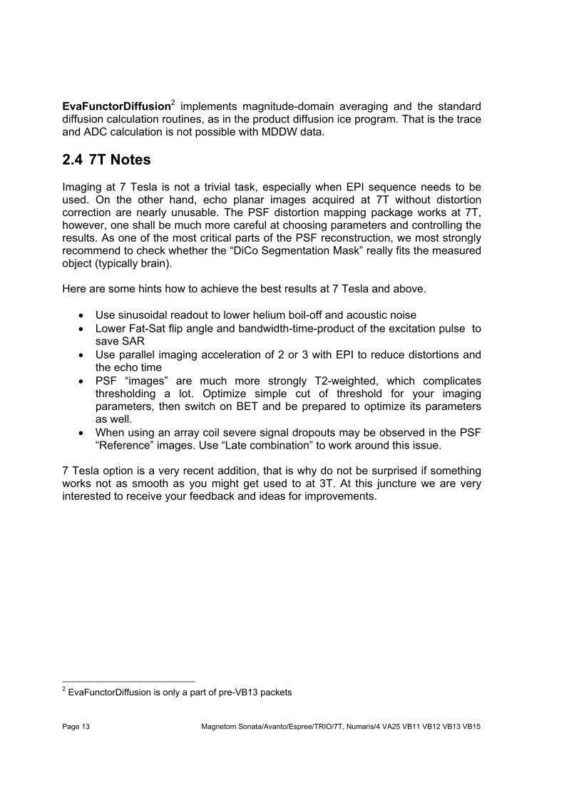
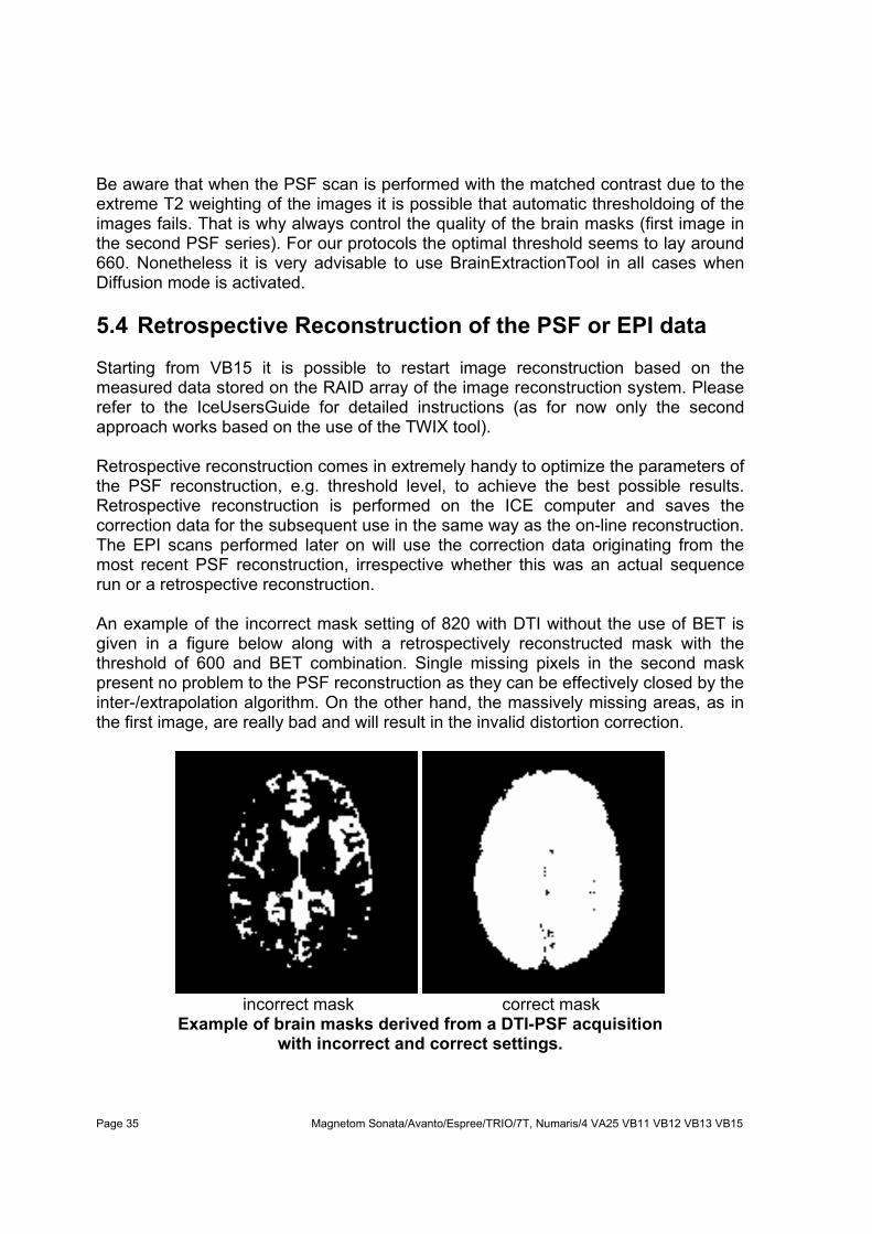
Be aware that when the PSF scan is performed with the matched contrast due to the extreme T2 weighting of the images it is possible that automatic thresholdoing of the images fails. That is why always control the quality of the brain masks (first image in the second PSF series). For our protocols the optimal threshold seems to lay around 660. Nonetheless it is very advisable to use BrainExtractionTool in all cases when Diffusion mode is activated. 5.4 Retrospective Reconstruction of the PSF or EPI data Starting from VB15 it is possible to restart image reconstruction based on the measured data stored on the RAID array of the image reconstruction system. Please refer to the IceUsersGuide for detailed instructions (as for now only the second approach works based on the use of the TWIX tool). Retrospective reconstruction comes in extremely handy to optimize the parameters of the PSF reconstruction, e.g. threshold level, to achieve the best possible results. Retrospective reconstruction is performed on the ICE computer and saves the correction data for the subsequent use in the same way as the on-line reconstruction. The EPI scans performed later on will use the correction data originating from the most recent PSF reconstruction, irrespective whether this was an actual sequence run or a retrospective reconstruction. An example of the incorrect mask setting of 820 with DTI without the use of BET is given in a figure below along with a retrospectively reconstructed mask with the threshold of 600 and BET combination. Single missing pixels in the second mask present no problem to the PSF reconstruction as they can be effectively closed by the inter-/extrapolation algorithm. On the other hand, the massively missing areas, as in the first image, are really bad and will result in the invalid distortion correction.

incorrect mask correct mask

Example of brain masks derived from a DTI-PSF acquisition with incorrect and correct settings.


It is also possible to repeat reconstruction of the EPI data retrospectively following the retrospective reconstruction of the PSF data e.g. to improve the correction quality or when the incorrect threshold setting was first discovered after the scan session. Keep in mind that the availability of the raw data on the RAID system depends on the load of the scanner and sequences being used. 5.5 Performing Distortion Correction Offline9 Offline distortion correction currently is not possible with diffusion datasets. Please note, that because of the very preliminary level of support in the actual Numaris versions, the offline execution of the EVA protocols may demand certain effort and may place certain requirements on the operator’s expertise. In any case we encourage the reader to study the related section of the ICE Users Guide, entitled “How to Perform Post Processing Evaluation on the HOST”, page 97. In order to be able to perform the offline distortion correction one has have a PSF dataset and at least one corresponding EPI dataset, both acquired in the same subject, with the same position, with the same imaging parameters and under the same shimming conditions. However, for the offline procession, it is possible to execute the PSF mapping method at the end of the session. It is also possible to use other EPI sequences, as long as the readout timing of the sequence used is equivalent to that of the PSF mapping technique. In order to perform corrections one has to first execute the PSF post-processing protocol (MrEvaPSF) on the PSF dataset. It is also possible then to control the expected quality of corrections and adjust the threshold parameter if needed. The PSF post-processing functor writes a set of files at C:\MedCom\, which are then used by the DiCo functor. After performing successfully the PSF EVA protocol it is possible to execute the DiCo protocol (MrEvaApplyMoCoDiCo). Keep in mind that the DiCo functor uses the reference and correction data stored by the PSF functor at C:\MedCom\. Known bug: as for version VA25 the off-line EVA framework reports wrong number of slices for the non-mosaic datasets, which makes it impossible to perform offlice correction of the single slice datasets.

9 Offline reconstruction is not yet available for VB13 and VB15

Date post:	31-Jan-2018
Category:	Documents
Upload:	vumien
View:	232 times
Download:	1 times

EPI Distortion Correction - mrdac.uni- · PDF fileEPI Distortion Correction Works-in-Progress...

Documents