AMERICAN JOURNA L OF EPIDEM[QLOGY Vol 121 No 2 Copyright copy 1985 by The Johns Hopkins University School of Hygiene and Public Health Printed in USA All righ t3 rt3er vti
Epidemiologic Programs for Computers and Calculators USE OF POISSON REGRESSION MODELS IN ESTIMATING
INCIDENCE RATES AND RATIOS
EDWARD L FROME AND H ARVEY CHECKOWAY
Frame E L (Oak Ridge National Laboratory Oak Ridge TN 37830) and H Checkoway Use of Poisson regression models in estimating incidence rates and ratios Am J Epidemio1985121309-23
Summarizing relative risk estimates across strata of a covariate is commonly done in comparative epidemiologic studies of incidence or mortality Conventional MantelmiddotHaenszel and rate standardization techniques used for this purpose are strictly suitable only when there is no interaction between relative risk and the covariate and tests for interaction typically are limited to examination for deparshytures from linearity Poisson regression modeling oIlers an alternative technique which can be used for summarizing relative risk and tor evaluating complex interactions with covariates A more general application of Poisson regression is its utility in modeling disease rates according to postulated etiologic mechanisms of exposures or according to disease expression characteristics in the population The applications of Poisson regression analysis to problems of summarizing relative risk and disease rate modeling are illustrated with examples of cancer incidence and mortality data including an example of a nonlinear model predicted by the multistage theory of carcinogenesis
biometry epidemiologic methods Poisson distribution regression analysis
Incidence or mortality data obtained from epidemiologic follow-up studies are often expressed as covariate stratum-spemiddot cific rates for which the covariate may be
Received for publication May 19 1983 and in fina l form May 15 1984
1 Mathematics and Statistics Research Engineershying Physics and Mathematics Division Oak Ridge National Laboratory Oak Ridge TN
2 Department of Epidemiology University of North Carolina School of Public Health Chapel Hill NC
Reprint requests to Dr Edward L Frome Oak Ridge Nationa l Laboratory PO Box Y Oak Ridge T N 37830
This report is based on work pe rformed under Contract DE-AC05-760R00033 with the US Departshyment of Energy Office of Health and Envi ronmental Research and the Oak Ridge Associated Universities and Contract W-7405-eng-26 with the Union Carbide Corporation
The aut hors are grateful to Drs Everett Logue Elaine Zeighami D G Goss lee and M D Morris for offering helpfu l suggestions and to Pamela Hooker for help with the manuscript
age or some other presumed confounding factor Comparative analysis of rates be shytween groups characterized according to ex shyposure level commonly involves computashytion of summary relative risk (or rate ratio) estimates wherein stratummiddotspecific relashytive risks are condensed into a single measure (1) Several methods have been proposed for this purpose The MantelshyHaenszel summary odds ratio method (2) has been adapted for use in cohort studies by Rothman and Boice (3) and by Tarone (4) Lilienfeld and Pyne (5) have also promiddot posed summarizing relative risk with a pro shycedure which differs from the previous apshyproaches principally in the choice of weights assigned to the stratummiddotspecific relative risk estimates Miettinen (6) has discussed this problem in the context of standardization as a means of controlling confounding
309
310 FROME AND CHECKOWA Y
With these relative risk summarizIng tech niques there is the implicit assumption that there is no interaction between relative risk and levels of the covariates and as such the comparison of summary estishymators is strictly valid only when this conshydit ion is true (7) Testing for interaction typically is limited to examining for deparshyture~ from lineari ty of relative risk howshyever when there are complex relationships between disease rates and the covariate conventional summary estimation techshyniques are unsuitable An alternative apshyproach to this problem is offered by modshyeling disease rates as a function of covariate levels Modeling disease rates can also be used for more general purposes such as to describe the pattern of disease occurrence according to postulated etiologic mechashynisms of exposure eg initiation and proshymotion activities of carcinogens or accordshying to disease expression characteristics in the population eg bimodal age distribushytion
In this paper we present a method for obtaining summary relative risk estimates by means of Poisson regression modeling Examples are presented to illustrate the method of summarizing relative risk and to demonstrate how Poisson regression can be used to address problems of heterogeneity and interaction An example that uses a nonlinear disease rate model derived from the multistage theory of carcinogenesis is given to illustrate the informativeness of the Poisson regression modeling approach
The Poisson regression model
The general framework of the Poisson regression model as applied to situations in which the dependent variable is a count (eg number of incident cases in a cohort study) has been described previously by Frome et al (8) The reader is referred to reference 9 for a discussion of the applicashytion of the model for epidemiologic analysis of cohort data To specify a Poisson regresshysion model it is assumed that the dependshyent va riable follows the Poisson distribushy
tion and t hat a rate function A(X J) that describes the relationship between disease rates the predictor variables (X) and the unknown vector of parameters (J) is given
In the context of a cohort study a popshyulation for which incidence or mortality data for some disease have been obtained can be categorized into J strata of the coshyvariate (eg age) for each of K risk (exshypoure) groups The data can be summashyrized for each level of these two factors as shown in table 1 where YJ denotes the number of cases and CJk t he number of persons or person-years for risk group kin stratum i The corresponding observed disshyease rate is rJ = YJcJbull If risk group 1 is considered to be the reference or nonexshyposed group the estimated relative risk for group k (k = 2 K) for stratum i (i =
1 J) is Tkr) 1
It is assumed that the YJ are distributed as Poisson variates (10 11) with expectashytion PJ = cJAJ The AJ represent the unshyderlying rate functions which are estimated from the data by rJbullbull If the covariate strashytum -specific relative risks are constant within each risk group then XJ = Ad where AJ denotes the rate for the ith strashytum level (Pk is the summary relative risk for group k (k gt 1) and = 1 for group k = 1 This is referred to as the product model and for estimation purposes it can be reshyparameterized as a log- linear model ie
A = exp(OJ + (5) (1)
where J = In(A) and 0 = In (k = 2
TABLE 1
Data layout for analysis of cohort study data
Risk group Stratum
2 k K
Cases Person-years
y c
y c
y c
y CoK
j Cases Person-years
Yjl
orgt Y) Cjj
Y 0
y ejK
J Cases Person-years
y 0
Yn en
Ybullbull c bullbull
Y K CK
311 POISSON REGRESSIO N MODELS FOR RATES
K) The J correspond to th e natural logashyrithms of the stratum-specific incidence rates in the reference group while the O represent the natural logarithm of t he sumshyma ry relative risk for group k (with group 1 as the reference group)
Tarone (4) has discussed the special case that occurs when there are only two risk groups and the more general case has been considered by Miett inen (6) Two of their examples will be given to illustrate how Poisson regression can be used to impleshyment and extend their analyses
Example 1- Relative risk estimation for two risk groups
This example illustrates how Poisson regression can be used when there are only two risk groups In this situation AJI = AJ and XJ2 = XJltgt = exp( aJ + 0) Scotto et al (12) compared skin cancer incidence rates among women for two geographic areas Dallas-Fort Worth and Minneapolis-St Paul Tarone (4) previously derived a sumshymary relative risk for Dallas-Fort Worth from the age -stratified data shown in table 2 T he formula Tarone used for the sumshymary relative risk in notation consistent with formulae given here is
J I J 11- (f c ) (f ZC 2 YJ I ) (2)Z Y J2
TABLE 2 Number of cases of non melanoma skin cancer and
population size for women in Dallo~-Fort Worth and MinneapolismiddotS t Paul
gtto Adapted from Scotto et a (12) t With Minneapolis-St Paul as the reference
group
where Cj = L CJk = total number of persons in the jth age stratum summed across K risk groups T arane computed a summary relative risk of 224 (standard deviation (SD) = 012) for these data with a X 2 for heterogeneity of 822 with 7 df indicating uniformity of relative risk across strata
The Poisson regresion model for these data (see Appendix for a discussion of the general case) can be expressed as
X(X fJ) = exp(XtJ )
= exp(~ XJJJ) = exp(J + 0) (3)
where X = (Xl X)) is a row vector and 1 = (a aK b) I In this example X I
through x are indicator variables repremiddot senting terms for each age stratum and X 9
indicates risk group so that 0 = In( ltgt) where ltgt denotes the summary relative risk for Dallas-Fort Worth with MinneapolisshySt Paul as the reference group Note that X is the ith row of the 16 by 9 model matrix X In general for a J by f table the model matrix will be J K by J + K - 1 A detailed discussion of a procedure used in construct ing a model matrix is given in the Appendix The maximum likelihood estishymate iJ of the parameter vector tJ is obshytained using the iterat ively reweighted least squares method desribed by Frome (9) The computations can be performed using the Generalized Linear Iterative Models (GUM) statistical package (13) (Listings of the computer program used for these analyses Can be obtained from t he author (E L F) on request)
The maximum likelihood estimate of 0 is amp= 0804 (the unadjusted estimate is 8= 0743) fro m which ~ = 223 is computed This result agrees closely with that obshytained from equation 2 by T arone (4) The estimated standard deviation for g is ob shytained from the inverse of the info rmation matrix which is readily available following the last iteration of the iteratively reo weighted least squares procedure The comshyputed standard deviation is 00522 which
312 FROME AND CHECKOWAY
gives a 95 per cent confidence interval for ltf of 202- 248 Heterogeneity of relative risk across strata is evaluated from the deviance D (~) which is a measure of unexshyplained variation (see Appendix) In this example D(~) = 8 17 with 7 df indicating that the product model cannot be rejected ie it is reasonable to assume that the relative risk is constant across age strata
A plot of the logarithm of the incidence rates against the log of age - 15 years (where age is the midpoint of the stratumshyspecific interval in yea rs) reveals that there is additional structure in these data (see figure 1) Figure 1 suggests that InA the natural logarithm of the age-specific rate increases linearly with lnt and the paramshyeter e is the slope of the line This is the relationship between incidence and age (t) that is predicted by the multistage theory of carcinogenesis (14) and is referred to as the power law because the age-specific inshycidence rates are proportional to t For the data in table 2- AI = Alit and AI = Autcent which can be wri tten as
A(X J ) = exp(x + Ox + oxd (4)
where XII = 1 X = In(t) and X I = 1 for Dallas-Fort Worth and 0 otherwise If t =
100
fO 0shy
f
0 0
~ ~
p
sect 0 10 Jr
~ CI
~ ))()J
bull
0001
1 10 00
AGE - 15
FIGURE 1 Logmiddotlog plot of age-specific incidence rates fo r skin cance r data for DaHas-Fort Worth (0---0) and MinneapolismiddotSt Paul (- ) (12)
(age - 15 years)3S then t = 1 for the 45shy54 age stratum and the intercept term in equation 4 is the logarithm of the incidence rate for Minneapolis-St Paul ie j = 4 (ages 45- 54) x = x = 0 and from equashytion 4 AO = exp(a) For Dallas -Fort Worth when ) = 4 and t = 1 AI = exp(a + 0) =
A()cent The maximum likelihood estimates for the parameters in equation 4 are amp =
- 0168 (SD = 0048) sect = 229 (SD = 0063) and S= 0803 (SD = 0052) The value for deviance which is asymptotically distribshyuted as a X 2 (8) is 1436 with 13 df indishycating a good fit of the power model for these data
The findings from the analysis described above are summarized in a Poisson ANOV A (analysis of variance) format in table 3 This table is obtained by recording the value of the deviance and the degrees of freedom for each model considered and can be used to evaluate the importance of parameters in the model and the goodness of fit of different models The deviance provides an absolute measure of residual (unexplained) variation and can be comshypared with the chi-square distribution to assess the goodness of fit of a specific model (The mean and variance of a chishysquare statistic are the degrees of freedom and two times the degrees of freedom reshyspectively)
As discussed previously the deviance of
TABLE 3 Pois8on ANOVA table lor skin cancer incidence data
in table 2
Model In( X) NOO[ Deviance df parame er f
Minimal 27903 15 Power law (0 ~ 0) ltr + Ot 2 2727 14
Age alone lt 8 2669 8 City alo ne a +h 2 25697 14 Power law 3 144 13( + Or + Age and city (IJ + b 9 82 7 Complete (yen)k 16 00
The deviance p rovides an abso lute measure of residual (ie unexplained) variation and is asymptotshyically dist ributed as a chi-square random variable (see Appendix)
313 POISSON IECIESSION
82 (df = 7) for the product model indicates that the relative risk is constant across age strata The deviance of the power law model (144 df = 13) further suggests a good fit of a model predicted by the multistage carshycinogenesis theory
Further inspection of table 3 indicates that there is considerable lack of fit for all other models considered in that the devishyance is considerably larger than the correshysponding degrees of freedom for each of these models In this situation the more parsimonious power law model is judged to provide a better representation of these data A more formal way to make this evalshyuation is to consider the difference of the deviances 144 - 82 = 62 This is a likelishyhood ratio statistic for the model ltX = ltX + e Int and can be compared with the chishysquare distribution with 13 - 7 = 6 df Comparison of the corresponding differshyences in the deviances and associated deshygrees of freedom suggests that the power model provides a good fit to the data
The importance of the parameter 0 can be evaluated by computing the decrease in the deviance that occurs when 0 is included in the power law model (2727 - 144) which is 2583 with 1 df This is consistent with the information obtained from the point estimate and its estimated standard deviashytion (amp SDb 2 = 2385) ie amp exceeds the null value of zero by more than 15 standard deviations The deviance can also be used to construct an R -type measure of variance explained For example the first three lines of table 3 show that most of the variation 100(27903 - 2669)27903 = 904 per cent in these data is explained by age alone and that the power law model (with 0 = 0) accounts for most (902 per cent ie 100(27903 - 2727)27903) of this exshyplained variation This example illustrates that the relative importance of various pashyrameters can be assessed in several ways using the Poisson ANOV A table and that these resulta are consistent with results obtained when point and interval estimates of summary relat ive risks are used We
MO[)ELS FOR RATES
emp hasize that this ad hoc analysis of the power law model should be interpreted as such and that a formal statistical test of the goodness of fit of a model that is obshytained after inspecting the data is of limited value The difference ofthe deviance should be used to assess the relative importance of a specific set of parameter values and is the analog of the decrease in sum of squares for standard linear models This implies that one should interpret the Poisson ANOV A in the same manner as an ANOVA table for an unbalanced design and it should be recognized that the results are order-dependent The general proce shydure that we recommend is to enter the potential confounding factor first and then to inspect the decrease in the deviance that occurs when the risk factor of interest is entered into the model as well as the deshyviance fo r the model with both factors inshycluded
In summary the analysis for this examshyple indicates that the relative risk for skin cancer among women is significantly higher in Dallas -Fort Worth than in Minneapolis shySt Paul that the relative risk is constant with respect to age and that the age-speshycific incidence rates are proportional to age - 15 years raised to the power of 23
Example 2- Relative risk estimation for K risk group
This next example is presented to demshyonstrate how Poisson regression modeling can be used to estimate the relative risk when there are more than two risk groups Miettinen (6) has discussed the general problem of summarizing relat ive risk in the context of standardization with respect to the distribution of a confounder The method of risk ratio standardization that Miettinen (6) used was illustrated with data from a cohort study by Kahn (15) of lung cancer mortality in relationship to cigarette smoking Table 4 shows the lung cancer death rates according to the levels of the risk factor and age the potential confounshyder
The crude relative risk (ie ignoring age
314 FRO ME AND CHECKOWA Y
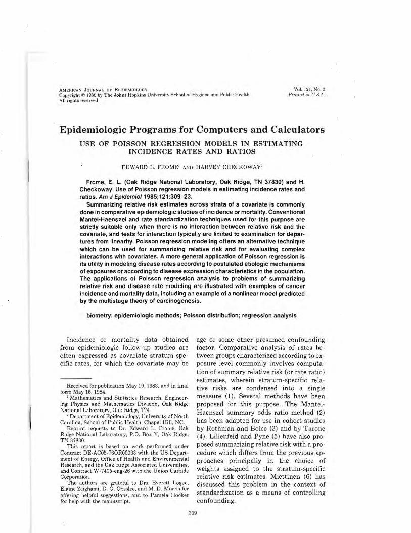
T ARt E 4 Lung cancer mortality according to cigarette consumption arid a~e for currenl cigarette smolwrs
Cigarettesday Age group Nonsmokers (yeArs) Occasional 1-9 10-20 21-39 40+
3)- 44 Dealhs Person -years (Rate per lOr )
0 35 164
(0)
0 3657
(0)
0 8 063
(0)
2 09965 (334)
4 40643 (984)
0 3992
(0)
45shy 54 Deaths P erson-years (Rate per lO)
0 1 5 1 ~4
(0)
deg 1283 (0)
0 3129
(0)
2 16392 (1 220)
10 12839 (7789)
2 1928
(10373)
55- 64 Deaths Person-years (Rate per 1O~)
~l
21388 (1169)
6 11624 (41113)
31 45217 (6856)
183 151664 (1 2066)
245 103020 (23782)
63 19649
(32063)
65- 74 Deaths Person -yea rs (Rate per 10~)
49 1712 11 (2862)
10 10053 (99 47)
44 371 30
(11850)
239 101731 (23493)
194 50045
(38765)
50 8937
(55947)
75+ Deaths Person-yea rs (Rate per 10~)
4 8489
(4712 )
1 5 12
(1953 1)
5 1923
(2600l)
15 3867
(387 89)
7 1273
(54988)
3 232
(129310)
Adapted from Kahn (15)
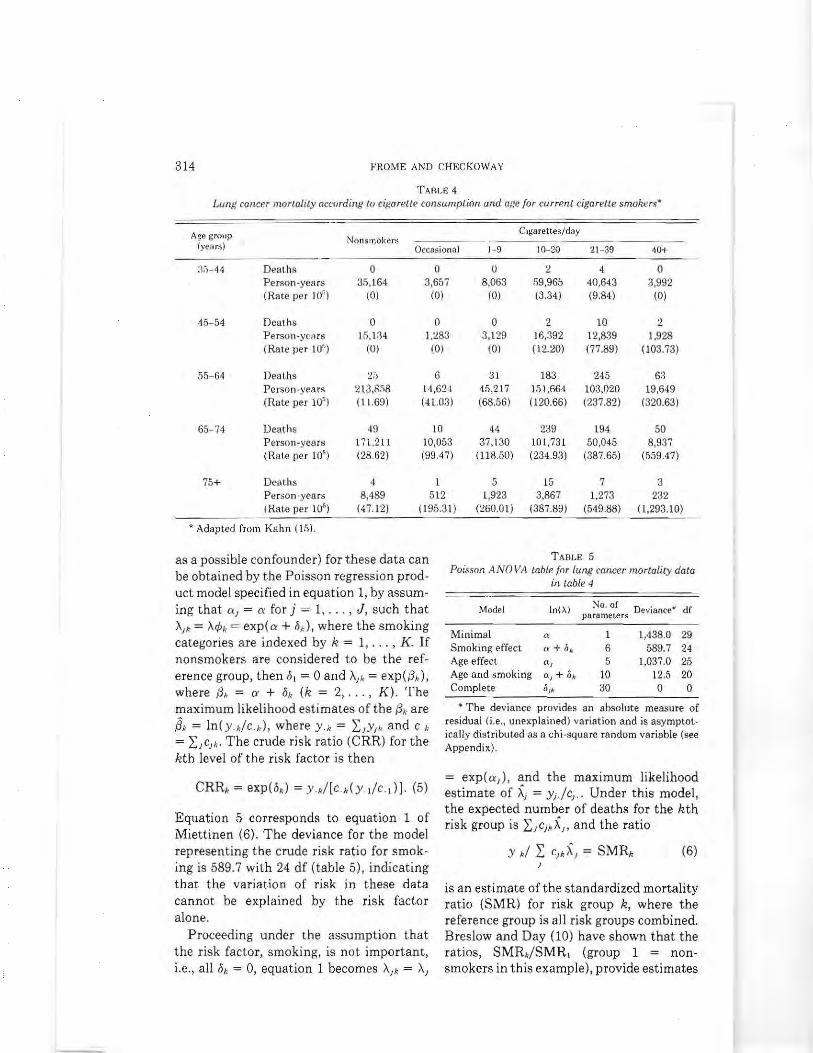
as a possible confounder) for t hese data can be obtained by the Poisson regression prodshyuct model specified in equation 1 by assumshying that I = for j = 1 J such that AI = Altgtk = exp(a + 0) where the smoking categories are indexed by k = 1 K If nonsmokers are considered to be the refshyerence group then 01 = degand AI = exp(O) where 0 = ex + Ok (k = 2 K) The maximum likelihood estimates of the Ok are S = In( yc) where Y = L Ylk and C
= I lcl The crude risk ratio (CRR) for the kth level of the risk factor is then
CRR = exp( b) = y[c (y c )] (5)
Equation 5 corresponds to equation 1 of Miettine n (6) The deviance for the model representing the crude risk ratio for smokshying is 5897 with 24 df (table 5) indicating that the variation of risk in these data cannot be explained by the risk factor alone
Proceeding under the assumption that the risk factor smoking is not important ie all I = 0 equation 1 becomes Ai = Al
T ABLE 5
Poiltson ANO VA lable fo r lung cancer mortality data in table 4
No ofModel in )) parameters Deviance df
Mi nimal a 1 14380 29 Smoking effect ~ + 1I~ 6 5897 24 Age effect a 5 10370 25 Age and smoking Ci j + 011 10 125 20 Complete 30 0 0
The deviance provides an absolute measure of residual (ie lInexplained) variation and is asymptotshyically distributed as a chi-squa re random variable (see Appendix)
= exp(a l ) and the maximum likelihood estimate of Xi = yi-cl Under this model the expected number of deaths for the kth risk group is I ICiXjgt and the ratio
y h I CIXI = SMRh (6)
is an estimate of the standardized mortality ratio (SMR) for risk group k where the reference group is all risk groups combined Breslow and Day (10) have shown that the ratios SMRSMR1 (group 1 = nonshysmokers in this example) provide estimates
315 POISSON REGRESSION MODELS FOR RATES
TABLE 6
Comparison of summary relative risk estimates for lung cancer data in lable 4
Crude risk ratio 32 48 75 126 193 SMRSMRt 34 48 88 157 219 ~ from product mode It 1 35 48 89 162 226
Reference category t All groups combined as the standard (see equation 6) SMR standardized mortality ratio t From Poisson regression model AJIt exp(aJ + Ih) where dk is the natural logarithm of the standardized
rate ratio ie 6~ = ln~k
of the summary relative risks These estishymates may be confounded however in that they lack a common standard The values of these ratios for the data in table 4 are given in table 6 The deviance for this model is 10370 with 25 df (see table 5) thus indicating that the confounder age alone cannot account fully for the variabilshyity in the data
From the foregoing it is apparent that neither smoking nor age alone can explain adequately the variation in these data A further analytic procedure is to fit the prodshyuct model equation (equation 1) which inshycludes both of these factors The maximum likelihood estimates for this model cannot be expressed in closed form therefore the iteratively reweighted least squares proceshydure is used to ohtain maximum likelihood estimates of the parameters (see Appenshydix) The deviance for this model is 125 with 20 df (table 5) indicating that the product model provides a very good descripshytion of these data
Miettinen (6) has proposed using the standardized risk ratio (SRR) as a sumshymary relative risk estimator The standardshyized risk ratio for risk group k is defined as
SRRk= (~ WIYlkClk) (~ wAI) (7)
where the WI are the standard population weights If the nonexposed risk group (k = 1) is considered to be the reference and the standard WI = Cjl and AJ = YJICjl When the product model provides a good fit as indicated by the contrast of the deviance
and its degrees of freedom the YJk in equashytion 7 can be replaced by their predicted values under the procJu~t model ie YJk = CJ exp(aJ + 0) = C)kAJrPk Thus the SRRk can be expressed as
SRRk = (~ wJJ cent) (~ WJI)
= centh = exp(b ) (8)
The ltPk are therefore estimators of the stanshydardized risk ratios with the nonexposed group as the referent and the choice of the standard population weights (wJ ) is unimshyportant In these situations we recommend use of the log-linear parameterized form of the product model as given in equation 1 because of ease of implementation with widely available statistical packages such as GLIM (13)
If the product model provides a reasonshyable fit to the data one can proceed to test the hypothesis of primary interest ie that the SRR = 1 for all k risk groups against the general alternative that SRR l This is equivalent to testing the hypothesis that Ii = 03 = = 0 = 0 in the product model In the example under consideration the test statistic is obtained by subtracting 125 from 10370 in table 5 to obtain 10245 with 5 df indicat ing that differences in standardized risk ratios are highly signifishycant
Example 3-Modeling disease rates according to levels of the exposure variable
and covariate
As mentioned previously summarizing relative risk across strata of a covariate is
316 FROME AND CHECKOWAY
appropriate when there is no interaction between relative risk and levels of the coshyvariates (7) In the context of the product model given in equation 1 interaction is equivalent to nonadditivity on a logarithshymic sca le and the deviance is used to meashysure the lack of fit of the product model In some situations an additive model Ak = AI + ltPh (ltPI = 0) may be more appropriate Note that the model matrix for this additive model is identical with that for the product model and Poisson regression can be used to fit either model When there are more complex relationships between the rates and the cQvariates conventional summary estimation techniques may not be approshypriate An alternative approach to this problem is offered by Poisson regression which can accommodate nonlinear modelshying of disease rates An example is given below to illustrate the approach
Doll (16) in studying the association beshytween cigarette smoki ng and lung cancer among British physicians proposed a model in which the age-specific death rate is proportional to smoking rate and age ie
A)k = (1 + adhll)t (9)
where t = (age - 20 years)425 and d =
exposure rate expressed as cigarettes per day Frome (9) has provided a detailed presshyentation of this model which is intrinsically nonlinear in the unknown parameter The parameter l represents the lung cancer death (per 105 man-years) in nonsmokers (d = 0) at age = 625 (t = 1) and It~ corresponds to the age-specific death rate in nonsmokers at age t A plot of the death rates against t on a log-log scale will result in a straight line with slope of 3 and intershycept l (see example 1) The effect of smokshying is represented by the term ad in equashytion 9 and when multiplied by t correshysponds to the increase in the lung cancer death rate for individuals that smoke d cigarettes per day Note that if 8 = 1 the relative increase in the age-specific death rate is proportional to the exposure rate for
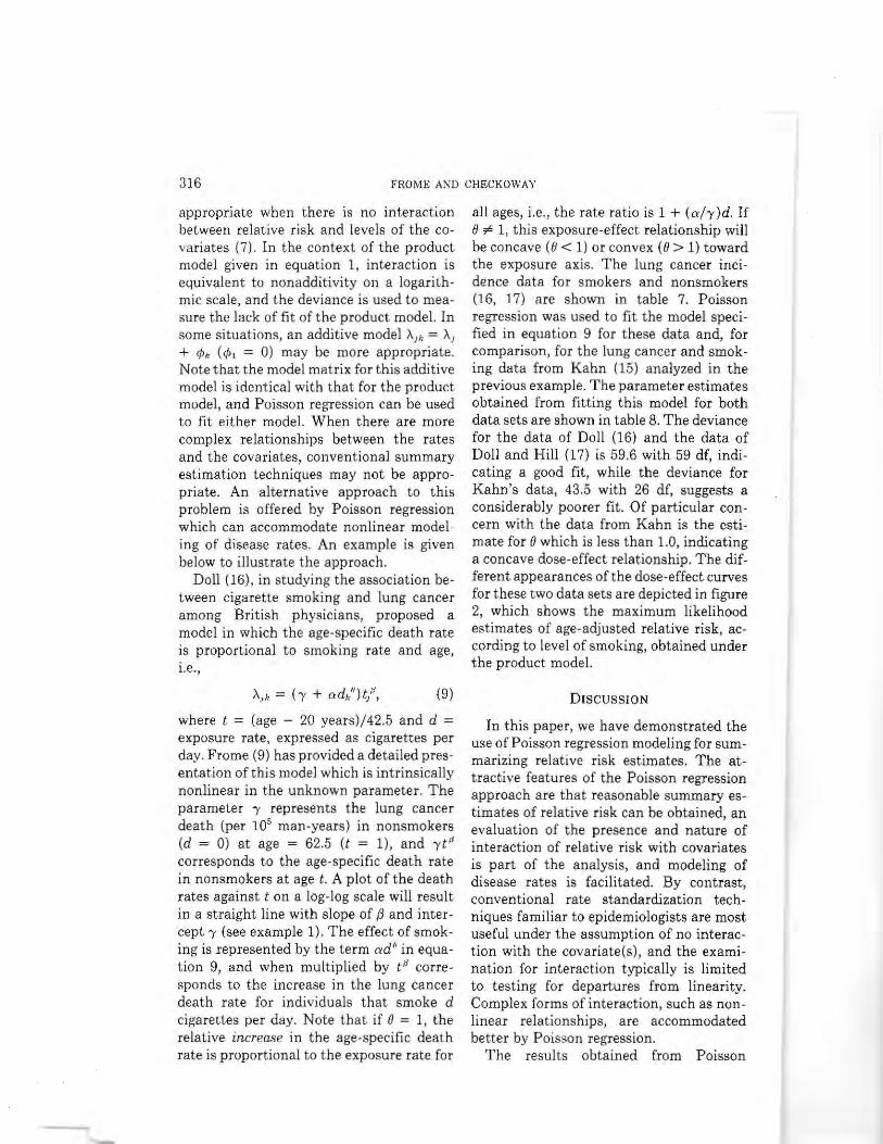
all ages ie the rate ratio is 1 + (ex-y )d If 8 1 this exposure-effect relationship will be concave (8 lt 1) or convex (8) 1) toward the exposure axis The lung cancer incishydence data for smokers and nonsmokers (16 17) are shown in table 7 Poisson regression was used to fit the model specishyfied in equation 9 for these data and for comparison for the lung cancer and smokshying data from Kahn (15) analyzed in the previous example The parameter estimates obtained from fitting this model for both data sets are shown in table 8 The deviance for the data of Doll (16) and the data of Doll and Hill (17) is 596 with 59 df indishycating a good fit while the deviance for Kahns data 435 with 26 df suggests a considerably poorer fit Of particular conshycern with the data from Kahn is the estishymate for 8 which is less than 10 indicating a concave dose-effect relationship The difshyferent appearances of the dose-effect curves for these two data sets are depicted in figure 2 which shows the maximum likelihood estimates of age-adjusted relative risk acshycording to level of smoking obtained under the product model
DISCUSSION
In this paper we have demonstrated the use of Poisson regression modeling for sumshymarizing relative risk estimates The atshytractive features of the Poisson regression approach are that reasonable summary esshytimates of relative risk can be obtained an evaluation of the presence and nature of interaction of relative risk with covariates is part of the analysis and modeling of disease rates is facilitated By contrast conventional rate standardization techshyniques familiar to epidemiologists are most useful under the assumption of no interacshytion with the covariate(s) and the examishynation for interaction typically is limited to testing for departures from linearity Complex forms of interaction such as nonshylinear relationships are accommodated better by Poisson regression
The resul ts obtained from Poisson
317 POISSON REGRESSION MODELS FOR RATES
TABLE 7
Person-years at risk and number of lung cancer cases (in parentheses) from study of British physiciansmiddot according to level of cigarette consumption
bull Death rate = XIII = (-y + ad )t where (age - 20 years)425 and d -= cigarettes per day
t Data from Kahn (15) t Data from Doll (16) and Doll and Hill (17) sect Standard deviation in parentheses
regression analysis are summarized in a Poisson ANOVA table which gives the deshyviances as measures of residual variation for the model parameters_ A general x test statistic for the null hypothesis of no efshy
J fect of the risk factor after adjustment for the effect of the covariate(s) can also be obtained from the ANOVA table (9) When this test is significant and there are quanshytitative val ues associated with levels of the exposure variable the covariate or both regression models can be developed to deshyscribe more precisely the relationships beshytween disease rates and the study factors
40
35
30
25 Q
amp I P ~ 201
or a I
oJ 1 Ej
sect I
I
$ 0 1 ltJ1 ~fi shy
p5
0 10 20 30 40 50
CIGARETTES PER DAY
FIGURE 2 Standardized risk ratios for tung cancer and level of c igarette smoking from studies of US veterans (0- - -0) (15) and British physicians (-- ) (16 17)
The flexibility of modeling offered by Poisshyson regression may facilitate comparisons of results from different studies when for example the levels of the exposure variashy
1
318 FROME AND CHECKOWA Y
bles differ between studies This situation was illustrated in example 3 in which an intrinsically nonlinear model was used to describe the effects of cigarette smoking on the age-specific mortality rates for lung cancer Data from two studies that used different exposure grouping schemes for age and smoking intensity were evaluated with the same regression model Although the examples considered here were limited to one risk factor and one covariate the methods described can be extended to inshyelude multiple risk factors and covariates simultaneously
The computational requirements for Poisson regression are sufficiently complex that in most situations a computer-based analysis would be required High quality inexpensive portable programs such as GLIM (13) are now widely available and can be used for all the analyses discussed in this paper (see Appendix for details) Poisson regression analysis can also be pershyformed on any micro (personal) computer with software that supports ANSI standard FORTRAN using the special purpose proshygram written by Frome (18) Consequently while the computations required for these methods are extensive by comparison with desk calculator or package program routines the computational complexities should no longer limit the availability and usefulness of Poisson regression analysis
Poisson regression models are especially appropriate in follow-up studies in which time-based denominators (person-years) are used to obtain disease rates or when the outcome of interest is rare such that the Poisson approximation to the binomial can be used (see Gart (19) for a discussion of this type of application) Further considshyeration of the use of generalized linear models for covariance adjustment and standardization is offered by Lane and NeIder (20) and Little and Pullum (21) Holford (ll) has provided an excellent reshyview of multiplicative models for rates and methods for analyzing categoric and censhysored survival data
The use of Poisson regression in cohorts with internal standard populations has been illustrated by Frome and Hudson (22) and by Lushbaugh et al (23) in occupashytional studies ofradiation-exposed workers Breslow et aL (24) have considered both internal and external standard populations in their demonstrations of the use of Poisshyson regression analysis and have discussed the Poisson regression approach relative to other statistical methods used in cohort studies When an external standard set of population rates is used eg national rates the eJk (see table 1) are expected events rather than person-years and although the c are in fact random the log-likelihood given under the Poisson assumption is still appropriate (24) Breslow (25) further disshycussed the use of Poisson regression with external rates and has illustrated how this multivariate approach can be used in relashytionship to traditional methods of cohort data analysis
The more general intrinsically nonlinear models are also of interest and can be hanshydled readily using the iteratively reweighted least squares procedure as was illustrated in example 3 James and Segal (26) have also described the fitting of intrinsically nonlinear models of age-year interaction effects to Poisson-distributed data Further discussion concerning the mathematical basis for regression methods appropriate to Poisson and binomial data is given by NeIder and Wedderburn (27) and Charnes et al (28) have detailed the underlying asshysumptions and applications of iteratively reweighted least squares model fitting for general regression models Frome (29) has recently reviewed the use of binomial and Poisson regression models in biomedical studies and a general overview of Poisson regression and its relationship to other esshytimation procedures has been presented by Koch et a (30)
Another useful feature of Poisson regresshysion analysis is the availability of regresshysion diagnostics that can be used to aid the analyst in detecting the outlying data
l
319 POISSON REGRESS(ON
points or inadequacies in the model specishyfication Pregibon (31) has described the essential elements of regression diagnostics for logistic regression and Frome (9) has discussed regression diagnostics for Poisshyson -distributed data
R EFERE NCES
1 Breslow NE Day NE Funda mental measures of disease occurrence and 8lsocia Lion Chap 2 In Statistical methods in cance r research analysis of case-control studies Volt Lyo n IARC 1980
2 Mantel N Haenszel W Stati stical aspects of the analysis of data from retrospective studies of disshyea )NC 195922719- 48
3 Rothman KJ Boice JD Epidemiologic analysis with a programmable calcu lato r Was hington DC N IH publication no 79middot 1649 1979 12- 13
4 Tarone RE On summa ry est imators of relati ve risk J Chronic Dis 198134463- 8
5 Lilienfeld DE Pyne DA On indices of morta lity deficiencies validi ty and alternatives J Chronic Dis 197932463-8
6 Miett inen OS Standa rdization of risk ratios Am J Epidemiol 197296383- 8
7 Kleinhau m DC Kupper LL Morgenstern H Epmiddot idemiologic research principles and quantit ative methods Belmont CA Lifet ime Learning Publishycations 1982320- 63
8 Frome EL Kutner MH Beauchamp JJ Regresmiddot sion analysis of Poisson-distributed data J Am Stat Assoc 197368935- 40
9 Frome EL The analys is of rates using Poisson regression models Biometrics 198339665- 74
10 Breslow NE Day NE Indi rect st andardization and multivariate models for rates with reference to the age adjustment of cancer incidence and relative frequency data J Chronic Dis 1975 28289- 303
11 Holford TR The ana lysis of rates and survivormiddot ship us ing logmiddot linea r models Biometrics 1980 36299- 305
12 Scotto J Kopf AW Urbach F Non-melanoma skin cancer a mong Caucasians in four a reas of the United States Cancer 197434 1333-8
13 Baker RJ Nelder JA Generali zed linear interacshytive modeling (GLlM) Release 3 Numerical Alshygorithms Group Oxford England 1978
14 Armitage P Doll R Stochastic models for carcinshyogenesis In Proceedings of the 4th Berkeley Symshyposium on Mathematical Statistics and Probabilshyity Biology and problems of health Vo14 Berkeshyley CA University of California Press 196119shy38
15 Kahn HA The Dorn study of smoking and morshytality among US vete rans repo rt on eight and one-half years of observatio n In Hae nszel W ed Epidemiological app roac hes to the study of cancer and other chronic diseases Nat Cancer Inst Monogr 19 1966 1- 125
16 Doll R The age distribtltion of cancer implicashytions for mode ls of ca rcinogenesis J R Stat Soc (A) 1971135133- 66
17 Doll R Hill AB Mortality o f Bri t ish doctors in
MODELS FOR RAT ES
rela t ion to smoking obse rvations on coronary thrombosis In Haenszel W ed Epidemiological approaches to the s tudy of cance r and other chronic diseases Nat Cancer Inst Monogr 19 1966205- 58
18 Frome EL Poisson regression analysis Am Stat shyistician 198135262- 3
19 Gart JJ The analysis of ratios and cross-product ratios of Poisson variates with application to inshycidence rates Communications Statist Theor Meth 1978A7(1O)9 l7- 37
20 Lane PW Nelder JA Analysis of covariance and standardization as instances of prediction Bioshymetrics 1982386 13- 21
21 Little RJA Pullum TW T he generailinear model and direct standardizat ion Socio l Meth Res 19797lt475- 50 l
22 Frome EL Hudson DR A ge neral statistical data structure for the epidemiologic studies of DOE workers In Truett T Margolies D Mensing RW eds Proceedings of t he 1980 Department of Energy Statistical Symposium CONF-801045 Berkeley CA 1981206- 18
23 Lushbaugh CC Fry SA S hy CM et a l DOE hea lth and mortali ty study at Oak Ridge In Proshyceedings of t he Health Physics Society sixteen th midyear topica l meeting CONF-83101 Albuquershyque NM 1983 105- 14
24 Breslow NE Lubin J H Marek P et a1 Multipli cative models and cohort analysis J Am Stut Assoc 1983781-12
25 Breslow N Multivariate cohort analysis JNCI (in press)
26 James JR Segal MR On a method of mortality analysis incorporating age -year in te raction with application to prostate cancer mort ality Biometmiddot rics 198238433-43
27 Neider JA Wedderbu rn RWM Gene ralized linear models J R Sta t Soc (A) 1972 135370-84
28 Charnes A Frome EL Yu PL The equivalence of generalized least squares and maximum likelihood estimation in the ex ponent ial family J Am S tat Assoc 197671169- 72
29 Frome EL Regression methods for bino mial and Poissonmiddotd istributed data In Herbert D ed Pro shyceedings of the American Association of Physimiddot cists in Medicine first midyear topical symposhysium Multiple regression analysis application in the health sciences (i n p ress)
30 Koch GC Atkinson SS Stokes ME Poisson regression In Kotz S Johnson LL Read A eds Encyclopedia of statistical sciences Vol 6 New York John Wiley amp Sons (in press )
31 Pregibon D Logistic regression diagnostics Ann Stat 19819705- 24
32 McCullagh P Quasi- likelihood functions Ann Stat 1983 11lt59- 67
33 Goodnight JH Sale J P SAS use rs guide stat is middot tics Cary NC SAS Institute 1982
34 Biomedica l Compu te r Progra ms P-Series (BMDP-79) Berkeley CA University of Califorshynia Press 1979
320 FROME AND CHECK OW A Y
ApPENDIX
Illustration of the model specification and computations involved in Poisson
regression analys is
The product model (see equation 1 and table 1) can be expressed as a log-linear model as follows
Aj = exp(a l + 0) = exp(Xp)
where X = (XI xp) is a row vector of indicator variables for the ith cell in the table and P = (a l (Xlgt 0 OK) is the p-dimensional column vector of un shyknown parameters with p = J + K - 1 If the ith cell of the table corresponds to raw j and column k the components of X (i = 1 JK) can be defined as follows
Xm = 1 if m == J
Xm = 1 if k gt 1 and m = J + k - 1
(m = 1 J + K - 1)
Xm = 0 otherwise
The rows of the JK by J + K - 1 X matrix for a J = 4 by K = 3 table are shown in Appendix table 1 to illustrate tbe general procedure
When ek gt 0 for allj and k this situation is equivalent to a full rank parameterizashytion of the design matrix for a two-factor fixed effects ANOV A model and the 0 are the natural logarithms of the standardized rate ratios with k = 1 as the standard and
reference group (see example 2) In pracshytice it is not necessary to generate this matrix because its structure is implied by the levels of the factors
Frome (9) has shown that maximum likelihood estimates of the parameter vecshytor P is equivalent to a weighted least squares regression Consider the following weighted sum of squares
N
S(P) = L wi [r - X(X P)] ~I
where r = yjCi denotes the observed rate in the ith cell (i = 1 N) where N is the number of cells in the table and the Poisson weights are Wi = cjX(X Pl The maximum likelihood estimate 13 is obtained using the iteratively reweighted least squares procedure and the deviance is comshyputed to obtain an absolute measure of residual (unexplained) variation The deshyviance is a likelihood ratio statistic-D (13) = -2[L(13) - L( y)] - where L(13) denotes the log-likelihood function evaluated at the maximum likelihood est imate and L( y) is the log-likelihood function for the satushyrated model ii =Yi (i = 1 N)
The deviance (see references 9 and 27) for a Poisson regression model is defined as follows
$SUBFILE DATA FCAPP1RSS ON 21 FEB 83 1 FCAPP1 APPENDIX LUNG CANCER MORTALITY-- AGE BY CIGARETTE CONSUMPTION I SOURCE KAHN(1966) APPENDIX TABLE A COLUMN 2 3 4 5 6 I NEVER OCCA 1-9 10-20 21-39 40+ $U NITS 30 $DATA C $READ C = MAN YEARS
8489 512 1923 3867 1273 232 $DATA Y $READ Y = LUNG CANCER DEATHS
000 240 o 0 0 2 10 2
25 6 31 183 245 63 49 10 44 239 194 50
4 1 5 15 7 3 $M TITLE FCAPP1 LUNG CANCER MORTALITY (KAHN1966) $E $CA $R=5 L=6 $FAC ROW R COL L $CA ROW=~GL(~RL) COL=$GL(~Ll) GENERATE ROW AND CO L $DATA 6 DOSE $READ 0 05 5 15 30 45 CIG PER DAY $CA D=DOSE(COL) AG= ROW10+30 DEFINE VARIABLES Xl AND X2 FOR NONLINEAR MODEL $WARN $CA Xl= IF( LE (D0)-8LOG(D) )$CA X2=LOG( (AG-20)425) $CA C=Cl00000 R=YC $PR TITLE R = LUNG CA DEATHS I 100000 MAN-YEARS $ $RETURN
FIGURE lAo GU M (1 3) program statements for defining data structure for Poisson regression analysis using the product model for data from Kahn (15) in example 2
I (Xi 3) denotes the regression function evaluated at tbe maximum likelibood estishymate iJ (Note tbat maximizing tbe logshylikelihood function is equivalent to minishymizing the deviance ) Anotber well known statistic tbat can be used as a measure of residual variation in Poisson regression is Pearson s X = L (y - iiol p (see refershyence 7) Botb of tbese test statistics will yield similar values wben tbe fitted values are large (ie p gt 3 for all i = 1 N) The value of these statistics may differ substantially wben some of the p are small and the analyst should proceed with caushytion If the assumed regression function I(X fJ) is appropriate both tbe deviance and Pearsons X will be distributed apshyproximately as a chi-square with N - pdf
where N is the number of observations and p is the number of parameters (see refershyences 8 and 32) It is generally advisable to utilize regression diagnostics (9 31) to asshysess the effect of outlying y values and or model inadequacies on these lack of fi t statistics and the estimated parameter valshyues In situations in which tbe unexplained variation is substantial t be lack of fit may be due to overdispersion (relative to tbe Poisson distribution) or to the inadequacy of tbe regression function If tbe lack of fit is attributed to overdispersion the estishymated parameter covariance matrix sbould be multiplied by tbe heterogeneity factor 1 = X(N - p) approximate interval estimates for the components of fJ should be based on the t distribution and test
322 FROME AND CHECKOWAY
$SUBFILE PHOD I $MAC PMOD I FIT PRODUCT MODEL $ERR P $WE C $YVAR R $FIT I $VAR ~L B2 II $CA II$CU(I) I $FIT COL $DISP E $USE RR I $FIT ROW $DISP E $USE RR $E $MAC RR I CALCULATE RISK RATIOS FOR PHOD
$EXTR $PE $CA BZ(II)PE(II ) B2(1)0 BZEXP(BZ) $PR RISK RATIOS B2 $END $R ETU RN I $SUBFILE NONLIN $HAC FITNL I FIT NONLINEAR MODEL DEFINED BY MAC NLH $DATA 4 B $READ 45 2 1 2 I STARTING VALUES FOR BETA $CA $K20 $C 000001 I SET CON CERGENCE CRITERIA $WE W tOWN Rl R2 R3 R4 $SC 1 $YVAR 2 DEFINE HODEL $WHILE $K NLM $PR STAND DEVS $DISP E $ $EXTR VL $CA H $VLW $DEL VI V2 PI P2 P3 P4 DB Z DELETE WOR K ARRAYS $PR H CONTAINS DIAG TERMS fROM H MATRIX $CA FT$SQRT( y) $SQRT( yl)-$ SQR T( 4CRHATl) $PR FT CONTAINS FREEMAN-TUKEY RESIDUALS $DEL NLH Rl R2 R3 $END $MACRO NLM POISSO N RATE ANALY SIS MACROS TO FIT NONLINEAR MODEL USING IRLS $CA VI $EXP ( B( I)X2) $CA V2 $IF( LE(D01l00HXP(B(2)B(3)Xl) ) $CA RHAT Vl( V2 EXP(B ( Qraquo ) $CA PI RHATX2 $CA P2 V2Vl $CA P3 P2Xl $CA P4 VlEXP(B(4 raquo $CA W CRHAT 2 R-RHAT LP Z $FIT PlP2P3+P4-GM $EXTR $PE $CA DB$PE $CA B B bull DB $PR $K ESTIMATES B I CHECK FOR CONVERGENCE OR MAXIMUM ITERATIONS $CA DBDBB DB IF( $LE(DBO)-DBDB) $CA DB $IF( LE(DBC)OI ) $CA $T $CU(DB) $CA $K$K-l $CA K $IF( LECUO) OK) $ $END MACROS REQUIRED BY OWN FOR POISSON RATE ANALYSIS I $H Rl $CA $FV$LP$E $M R2 $CA DRl0 $E $M R3 $CA VAl O$E $M R4 $CA $DI 2( Y$LOG(RRHAT)-CZ) W $E I $RETURN
FIGURE 2A GLlM (13) program statements for Poisson regression analysis of Kahns (15) data using the product model (example 2) and the nonlinear model in equation 9 (example 3)
statist ics for the relative importance of subshy factors that correspond to age and smoking sets of parameters should be based on apshy respectively The values of these factors proximate F ratios (see references 8 and and the variables Xl and X2 that are 32) needed for the nonlinear model are genershy
Figure lA provides a listing ofthe GLIM ated in the last 10 lines of figure lAo The (13) program statements that were used for GLIM macro PMOD in figure 2A was used the analysis of the data in example 2 from for the analysis of the data from example 2 Kahn (15) The GLIM statements in figure using the product model lA read the number of person-years into The data from example 3 necessitated the vector C and the corresponding number use of a model which is nonlinear in its of lung cancer deaths into the vector Y In parameter (equation 9) and therefore canshyGLIM terminology ROWand COL are not be fitted to these data with standard
1
323 POISSON REGRESSION
GLIM options Maximum likelihood estishymates of the model parameters can be obshytained from the iteratively reweigh ted linshyear squares algorithm using a G LIM macro developed for this purpose (9) The GLIM macro statements for fitting this nonlinear model are shown in figure 2A The iterashytively reweighted linear squares estimation method requires the partial derivatives of the rate function
X(Xi J) = [exp(J + Jxd
+ exp(34)J exp(3x)
where Xi = In (d) (d = dose rate) x = log(t) and J = (13 Ina 0 In-y) The partial
MODELS FOR RATES
derivatives are defined in the GLIM macro NLM (see figure 2A) as Pl P2 P3 and P4 where for example PI is
Pl = aX(X J)a 3
=x [V2 + exp(3)]Vl
where V2 = exp(p + Px d and Vl = exp(px) Additional macros that are reshyquired for the nonlinear model are also listed in figure 2A and the reader is reshyferred to the GLIM manual (13 Chap 18) for further details Identical results can also be obtained using the FORTRAN program PREG (18) the SAS procedure NLIN (33) and the BMDP program P3R (34)
310 FROME AND CHECKOWA Y
With these relative risk summarizIng tech niques there is the implicit assumption that there is no interaction between relative risk and levels of the covariates and as such the comparison of summary estishymators is strictly valid only when this conshydit ion is true (7) Testing for interaction typically is limited to examining for deparshyture~ from lineari ty of relative risk howshyever when there are complex relationships between disease rates and the covariate conventional summary estimation techshyniques are unsuitable An alternative apshyproach to this problem is offered by modshyeling disease rates as a function of covariate levels Modeling disease rates can also be used for more general purposes such as to describe the pattern of disease occurrence according to postulated etiologic mechashynisms of exposure eg initiation and proshymotion activities of carcinogens or accordshying to disease expression characteristics in the population eg bimodal age distribushytion
In this paper we present a method for obtaining summary relative risk estimates by means of Poisson regression modeling Examples are presented to illustrate the method of summarizing relative risk and to demonstrate how Poisson regression can be used to address problems of heterogeneity and interaction An example that uses a nonlinear disease rate model derived from the multistage theory of carcinogenesis is given to illustrate the informativeness of the Poisson regression modeling approach
The Poisson regression model
The general framework of the Poisson regression model as applied to situations in which the dependent variable is a count (eg number of incident cases in a cohort study) has been described previously by Frome et al (8) The reader is referred to reference 9 for a discussion of the applicashytion of the model for epidemiologic analysis of cohort data To specify a Poisson regresshysion model it is assumed that the dependshyent va riable follows the Poisson distribushy
tion and t hat a rate function A(X J) that describes the relationship between disease rates the predictor variables (X) and the unknown vector of parameters (J) is given
In the context of a cohort study a popshyulation for which incidence or mortality data for some disease have been obtained can be categorized into J strata of the coshyvariate (eg age) for each of K risk (exshypoure) groups The data can be summashyrized for each level of these two factors as shown in table 1 where YJ denotes the number of cases and CJk t he number of persons or person-years for risk group kin stratum i The corresponding observed disshyease rate is rJ = YJcJbull If risk group 1 is considered to be the reference or nonexshyposed group the estimated relative risk for group k (k = 2 K) for stratum i (i =
1 J) is Tkr) 1
It is assumed that the YJ are distributed as Poisson variates (10 11) with expectashytion PJ = cJAJ The AJ represent the unshyderlying rate functions which are estimated from the data by rJbullbull If the covariate strashytum -specific relative risks are constant within each risk group then XJ = Ad where AJ denotes the rate for the ith strashytum level (Pk is the summary relative risk for group k (k gt 1) and = 1 for group k = 1 This is referred to as the product model and for estimation purposes it can be reshyparameterized as a log- linear model ie
A = exp(OJ + (5) (1)
where J = In(A) and 0 = In (k = 2
TABLE 1
Data layout for analysis of cohort study data
Risk group Stratum
2 k K
Cases Person-years
y c
y c
y c
y CoK
j Cases Person-years
Yjl
orgt Y) Cjj
Y 0
y ejK
J Cases Person-years
y 0
Yn en
Ybullbull c bullbull
Y K CK
311 POISSON REGRESSIO N MODELS FOR RATES
K) The J correspond to th e natural logashyrithms of the stratum-specific incidence rates in the reference group while the O represent the natural logarithm of t he sumshyma ry relative risk for group k (with group 1 as the reference group)
Tarone (4) has discussed the special case that occurs when there are only two risk groups and the more general case has been considered by Miett inen (6) Two of their examples will be given to illustrate how Poisson regression can be used to impleshyment and extend their analyses
Example 1- Relative risk estimation for two risk groups
This example illustrates how Poisson regression can be used when there are only two risk groups In this situation AJI = AJ and XJ2 = XJltgt = exp( aJ + 0) Scotto et al (12) compared skin cancer incidence rates among women for two geographic areas Dallas-Fort Worth and Minneapolis-St Paul Tarone (4) previously derived a sumshymary relative risk for Dallas-Fort Worth from the age -stratified data shown in table 2 T he formula Tarone used for the sumshymary relative risk in notation consistent with formulae given here is
J I J 11- (f c ) (f ZC 2 YJ I ) (2)Z Y J2
TABLE 2 Number of cases of non melanoma skin cancer and
population size for women in Dallo~-Fort Worth and MinneapolismiddotS t Paul
gtto Adapted from Scotto et a (12) t With Minneapolis-St Paul as the reference
group
where Cj = L CJk = total number of persons in the jth age stratum summed across K risk groups T arane computed a summary relative risk of 224 (standard deviation (SD) = 012) for these data with a X 2 for heterogeneity of 822 with 7 df indicating uniformity of relative risk across strata
The Poisson regresion model for these data (see Appendix for a discussion of the general case) can be expressed as
X(X fJ) = exp(XtJ )
= exp(~ XJJJ) = exp(J + 0) (3)
where X = (Xl X)) is a row vector and 1 = (a aK b) I In this example X I
through x are indicator variables repremiddot senting terms for each age stratum and X 9
indicates risk group so that 0 = In( ltgt) where ltgt denotes the summary relative risk for Dallas-Fort Worth with MinneapolisshySt Paul as the reference group Note that X is the ith row of the 16 by 9 model matrix X In general for a J by f table the model matrix will be J K by J + K - 1 A detailed discussion of a procedure used in construct ing a model matrix is given in the Appendix The maximum likelihood estishymate iJ of the parameter vector tJ is obshytained using the iterat ively reweighted least squares method desribed by Frome (9) The computations can be performed using the Generalized Linear Iterative Models (GUM) statistical package (13) (Listings of the computer program used for these analyses Can be obtained from t he author (E L F) on request)
The maximum likelihood estimate of 0 is amp= 0804 (the unadjusted estimate is 8= 0743) fro m which ~ = 223 is computed This result agrees closely with that obshytained from equation 2 by T arone (4) The estimated standard deviation for g is ob shytained from the inverse of the info rmation matrix which is readily available following the last iteration of the iteratively reo weighted least squares procedure The comshyputed standard deviation is 00522 which
312 FROME AND CHECKOWAY
gives a 95 per cent confidence interval for ltf of 202- 248 Heterogeneity of relative risk across strata is evaluated from the deviance D (~) which is a measure of unexshyplained variation (see Appendix) In this example D(~) = 8 17 with 7 df indicating that the product model cannot be rejected ie it is reasonable to assume that the relative risk is constant across age strata
A plot of the logarithm of the incidence rates against the log of age - 15 years (where age is the midpoint of the stratumshyspecific interval in yea rs) reveals that there is additional structure in these data (see figure 1) Figure 1 suggests that InA the natural logarithm of the age-specific rate increases linearly with lnt and the paramshyeter e is the slope of the line This is the relationship between incidence and age (t) that is predicted by the multistage theory of carcinogenesis (14) and is referred to as the power law because the age-specific inshycidence rates are proportional to t For the data in table 2- AI = Alit and AI = Autcent which can be wri tten as
A(X J ) = exp(x + Ox + oxd (4)
where XII = 1 X = In(t) and X I = 1 for Dallas-Fort Worth and 0 otherwise If t =
100
fO 0shy
f
0 0
~ ~
p
sect 0 10 Jr
~ CI
~ ))()J
bull
0001
1 10 00
AGE - 15
FIGURE 1 Logmiddotlog plot of age-specific incidence rates fo r skin cance r data for DaHas-Fort Worth (0---0) and MinneapolismiddotSt Paul (- ) (12)
(age - 15 years)3S then t = 1 for the 45shy54 age stratum and the intercept term in equation 4 is the logarithm of the incidence rate for Minneapolis-St Paul ie j = 4 (ages 45- 54) x = x = 0 and from equashytion 4 AO = exp(a) For Dallas -Fort Worth when ) = 4 and t = 1 AI = exp(a + 0) =
A()cent The maximum likelihood estimates for the parameters in equation 4 are amp =
- 0168 (SD = 0048) sect = 229 (SD = 0063) and S= 0803 (SD = 0052) The value for deviance which is asymptotically distribshyuted as a X 2 (8) is 1436 with 13 df indishycating a good fit of the power model for these data
The findings from the analysis described above are summarized in a Poisson ANOV A (analysis of variance) format in table 3 This table is obtained by recording the value of the deviance and the degrees of freedom for each model considered and can be used to evaluate the importance of parameters in the model and the goodness of fit of different models The deviance provides an absolute measure of residual (unexplained) variation and can be comshypared with the chi-square distribution to assess the goodness of fit of a specific model (The mean and variance of a chishysquare statistic are the degrees of freedom and two times the degrees of freedom reshyspectively)
As discussed previously the deviance of
TABLE 3 Pois8on ANOVA table lor skin cancer incidence data
in table 2
Model In( X) NOO[ Deviance df parame er f
Minimal 27903 15 Power law (0 ~ 0) ltr + Ot 2 2727 14
Age alone lt 8 2669 8 City alo ne a +h 2 25697 14 Power law 3 144 13( + Or + Age and city (IJ + b 9 82 7 Complete (yen)k 16 00
The deviance p rovides an abso lute measure of residual (ie unexplained) variation and is asymptotshyically dist ributed as a chi-square random variable (see Appendix)
313 POISSON IECIESSION
82 (df = 7) for the product model indicates that the relative risk is constant across age strata The deviance of the power law model (144 df = 13) further suggests a good fit of a model predicted by the multistage carshycinogenesis theory
Further inspection of table 3 indicates that there is considerable lack of fit for all other models considered in that the devishyance is considerably larger than the correshysponding degrees of freedom for each of these models In this situation the more parsimonious power law model is judged to provide a better representation of these data A more formal way to make this evalshyuation is to consider the difference of the deviances 144 - 82 = 62 This is a likelishyhood ratio statistic for the model ltX = ltX + e Int and can be compared with the chishysquare distribution with 13 - 7 = 6 df Comparison of the corresponding differshyences in the deviances and associated deshygrees of freedom suggests that the power model provides a good fit to the data
The importance of the parameter 0 can be evaluated by computing the decrease in the deviance that occurs when 0 is included in the power law model (2727 - 144) which is 2583 with 1 df This is consistent with the information obtained from the point estimate and its estimated standard deviashytion (amp SDb 2 = 2385) ie amp exceeds the null value of zero by more than 15 standard deviations The deviance can also be used to construct an R -type measure of variance explained For example the first three lines of table 3 show that most of the variation 100(27903 - 2669)27903 = 904 per cent in these data is explained by age alone and that the power law model (with 0 = 0) accounts for most (902 per cent ie 100(27903 - 2727)27903) of this exshyplained variation This example illustrates that the relative importance of various pashyrameters can be assessed in several ways using the Poisson ANOV A table and that these resulta are consistent with results obtained when point and interval estimates of summary relat ive risks are used We
MO[)ELS FOR RATES
emp hasize that this ad hoc analysis of the power law model should be interpreted as such and that a formal statistical test of the goodness of fit of a model that is obshytained after inspecting the data is of limited value The difference ofthe deviance should be used to assess the relative importance of a specific set of parameter values and is the analog of the decrease in sum of squares for standard linear models This implies that one should interpret the Poisson ANOV A in the same manner as an ANOVA table for an unbalanced design and it should be recognized that the results are order-dependent The general proce shydure that we recommend is to enter the potential confounding factor first and then to inspect the decrease in the deviance that occurs when the risk factor of interest is entered into the model as well as the deshyviance fo r the model with both factors inshycluded
In summary the analysis for this examshyple indicates that the relative risk for skin cancer among women is significantly higher in Dallas -Fort Worth than in Minneapolis shySt Paul that the relative risk is constant with respect to age and that the age-speshycific incidence rates are proportional to age - 15 years raised to the power of 23
Example 2- Relative risk estimation for K risk group
This next example is presented to demshyonstrate how Poisson regression modeling can be used to estimate the relative risk when there are more than two risk groups Miettinen (6) has discussed the general problem of summarizing relat ive risk in the context of standardization with respect to the distribution of a confounder The method of risk ratio standardization that Miettinen (6) used was illustrated with data from a cohort study by Kahn (15) of lung cancer mortality in relationship to cigarette smoking Table 4 shows the lung cancer death rates according to the levels of the risk factor and age the potential confounshyder
The crude relative risk (ie ignoring age
314 FRO ME AND CHECKOWA Y
T ARt E 4 Lung cancer mortality according to cigarette consumption arid a~e for currenl cigarette smolwrs
Cigarettesday Age group Nonsmokers (yeArs) Occasional 1-9 10-20 21-39 40+
3)- 44 Dealhs Person -years (Rate per lOr )
0 35 164
(0)
0 3657
(0)
0 8 063
(0)
2 09965 (334)
4 40643 (984)
0 3992
(0)
45shy 54 Deaths P erson-years (Rate per lO)
0 1 5 1 ~4
(0)
deg 1283 (0)
0 3129
(0)
2 16392 (1 220)
10 12839 (7789)
2 1928
(10373)
55- 64 Deaths Person-years (Rate per 1O~)
~l
21388 (1169)
6 11624 (41113)
31 45217 (6856)
183 151664 (1 2066)
245 103020 (23782)
63 19649
(32063)
65- 74 Deaths Person -yea rs (Rate per 10~)
49 1712 11 (2862)
10 10053 (99 47)
44 371 30
(11850)
239 101731 (23493)
194 50045
(38765)
50 8937
(55947)
75+ Deaths Person-yea rs (Rate per 10~)
4 8489
(4712 )
1 5 12
(1953 1)
5 1923
(2600l)
15 3867
(387 89)
7 1273
(54988)
3 232
(129310)
Adapted from Kahn (15)
as a possible confounder) for t hese data can be obtained by the Poisson regression prodshyuct model specified in equation 1 by assumshying that I = for j = 1 J such that AI = Altgtk = exp(a + 0) where the smoking categories are indexed by k = 1 K If nonsmokers are considered to be the refshyerence group then 01 = degand AI = exp(O) where 0 = ex + Ok (k = 2 K) The maximum likelihood estimates of the Ok are S = In( yc) where Y = L Ylk and C
= I lcl The crude risk ratio (CRR) for the kth level of the risk factor is then
CRR = exp( b) = y[c (y c )] (5)
Equation 5 corresponds to equation 1 of Miettine n (6) The deviance for the model representing the crude risk ratio for smokshying is 5897 with 24 df (table 5) indicating that the variation of risk in these data cannot be explained by the risk factor alone
Proceeding under the assumption that the risk factor smoking is not important ie all I = 0 equation 1 becomes Ai = Al
T ABLE 5
Poiltson ANO VA lable fo r lung cancer mortality data in table 4
No ofModel in )) parameters Deviance df
Mi nimal a 1 14380 29 Smoking effect ~ + 1I~ 6 5897 24 Age effect a 5 10370 25 Age and smoking Ci j + 011 10 125 20 Complete 30 0 0
The deviance provides an absolute measure of residual (ie lInexplained) variation and is asymptotshyically distributed as a chi-squa re random variable (see Appendix)
= exp(a l ) and the maximum likelihood estimate of Xi = yi-cl Under this model the expected number of deaths for the kth risk group is I ICiXjgt and the ratio
y h I CIXI = SMRh (6)
is an estimate of the standardized mortality ratio (SMR) for risk group k where the reference group is all risk groups combined Breslow and Day (10) have shown that the ratios SMRSMR1 (group 1 = nonshysmokers in this example) provide estimates
315 POISSON REGRESSION MODELS FOR RATES
TABLE 6
Comparison of summary relative risk estimates for lung cancer data in lable 4
Crude risk ratio 32 48 75 126 193 SMRSMRt 34 48 88 157 219 ~ from product mode It 1 35 48 89 162 226
Reference category t All groups combined as the standard (see equation 6) SMR standardized mortality ratio t From Poisson regression model AJIt exp(aJ + Ih) where dk is the natural logarithm of the standardized
rate ratio ie 6~ = ln~k
of the summary relative risks These estishymates may be confounded however in that they lack a common standard The values of these ratios for the data in table 4 are given in table 6 The deviance for this model is 10370 with 25 df (see table 5) thus indicating that the confounder age alone cannot account fully for the variabilshyity in the data
From the foregoing it is apparent that neither smoking nor age alone can explain adequately the variation in these data A further analytic procedure is to fit the prodshyuct model equation (equation 1) which inshycludes both of these factors The maximum likelihood estimates for this model cannot be expressed in closed form therefore the iteratively reweighted least squares proceshydure is used to ohtain maximum likelihood estimates of the parameters (see Appenshydix) The deviance for this model is 125 with 20 df (table 5) indicating that the product model provides a very good descripshytion of these data
Miettinen (6) has proposed using the standardized risk ratio (SRR) as a sumshymary relative risk estimator The standardshyized risk ratio for risk group k is defined as
SRRk= (~ WIYlkClk) (~ wAI) (7)
where the WI are the standard population weights If the nonexposed risk group (k = 1) is considered to be the reference and the standard WI = Cjl and AJ = YJICjl When the product model provides a good fit as indicated by the contrast of the deviance
and its degrees of freedom the YJk in equashytion 7 can be replaced by their predicted values under the procJu~t model ie YJk = CJ exp(aJ + 0) = C)kAJrPk Thus the SRRk can be expressed as
SRRk = (~ wJJ cent) (~ WJI)
= centh = exp(b ) (8)
The ltPk are therefore estimators of the stanshydardized risk ratios with the nonexposed group as the referent and the choice of the standard population weights (wJ ) is unimshyportant In these situations we recommend use of the log-linear parameterized form of the product model as given in equation 1 because of ease of implementation with widely available statistical packages such as GLIM (13)
If the product model provides a reasonshyable fit to the data one can proceed to test the hypothesis of primary interest ie that the SRR = 1 for all k risk groups against the general alternative that SRR l This is equivalent to testing the hypothesis that Ii = 03 = = 0 = 0 in the product model In the example under consideration the test statistic is obtained by subtracting 125 from 10370 in table 5 to obtain 10245 with 5 df indicat ing that differences in standardized risk ratios are highly signifishycant
Example 3-Modeling disease rates according to levels of the exposure variable
and covariate
As mentioned previously summarizing relative risk across strata of a covariate is
316 FROME AND CHECKOWAY
appropriate when there is no interaction between relative risk and levels of the coshyvariates (7) In the context of the product model given in equation 1 interaction is equivalent to nonadditivity on a logarithshymic sca le and the deviance is used to meashysure the lack of fit of the product model In some situations an additive model Ak = AI + ltPh (ltPI = 0) may be more appropriate Note that the model matrix for this additive model is identical with that for the product model and Poisson regression can be used to fit either model When there are more complex relationships between the rates and the cQvariates conventional summary estimation techniques may not be approshypriate An alternative approach to this problem is offered by Poisson regression which can accommodate nonlinear modelshying of disease rates An example is given below to illustrate the approach
Doll (16) in studying the association beshytween cigarette smoki ng and lung cancer among British physicians proposed a model in which the age-specific death rate is proportional to smoking rate and age ie
A)k = (1 + adhll)t (9)
where t = (age - 20 years)425 and d =
exposure rate expressed as cigarettes per day Frome (9) has provided a detailed presshyentation of this model which is intrinsically nonlinear in the unknown parameter The parameter l represents the lung cancer death (per 105 man-years) in nonsmokers (d = 0) at age = 625 (t = 1) and It~ corresponds to the age-specific death rate in nonsmokers at age t A plot of the death rates against t on a log-log scale will result in a straight line with slope of 3 and intershycept l (see example 1) The effect of smokshying is represented by the term ad in equashytion 9 and when multiplied by t correshysponds to the increase in the lung cancer death rate for individuals that smoke d cigarettes per day Note that if 8 = 1 the relative increase in the age-specific death rate is proportional to the exposure rate for
all ages ie the rate ratio is 1 + (ex-y )d If 8 1 this exposure-effect relationship will be concave (8 lt 1) or convex (8) 1) toward the exposure axis The lung cancer incishydence data for smokers and nonsmokers (16 17) are shown in table 7 Poisson regression was used to fit the model specishyfied in equation 9 for these data and for comparison for the lung cancer and smokshying data from Kahn (15) analyzed in the previous example The parameter estimates obtained from fitting this model for both data sets are shown in table 8 The deviance for the data of Doll (16) and the data of Doll and Hill (17) is 596 with 59 df indishycating a good fit while the deviance for Kahns data 435 with 26 df suggests a considerably poorer fit Of particular conshycern with the data from Kahn is the estishymate for 8 which is less than 10 indicating a concave dose-effect relationship The difshyferent appearances of the dose-effect curves for these two data sets are depicted in figure 2 which shows the maximum likelihood estimates of age-adjusted relative risk acshycording to level of smoking obtained under the product model
DISCUSSION
In this paper we have demonstrated the use of Poisson regression modeling for sumshymarizing relative risk estimates The atshytractive features of the Poisson regression approach are that reasonable summary esshytimates of relative risk can be obtained an evaluation of the presence and nature of interaction of relative risk with covariates is part of the analysis and modeling of disease rates is facilitated By contrast conventional rate standardization techshyniques familiar to epidemiologists are most useful under the assumption of no interacshytion with the covariate(s) and the examishynation for interaction typically is limited to testing for departures from linearity Complex forms of interaction such as nonshylinear relationships are accommodated better by Poisson regression
The resul ts obtained from Poisson
317 POISSON REGRESSION MODELS FOR RATES
TABLE 7
Person-years at risk and number of lung cancer cases (in parentheses) from study of British physiciansmiddot according to level of cigarette consumption
bull Death rate = XIII = (-y + ad )t where (age - 20 years)425 and d -= cigarettes per day
t Data from Kahn (15) t Data from Doll (16) and Doll and Hill (17) sect Standard deviation in parentheses
regression analysis are summarized in a Poisson ANOVA table which gives the deshyviances as measures of residual variation for the model parameters_ A general x test statistic for the null hypothesis of no efshy
J fect of the risk factor after adjustment for the effect of the covariate(s) can also be obtained from the ANOVA table (9) When this test is significant and there are quanshytitative val ues associated with levels of the exposure variable the covariate or both regression models can be developed to deshyscribe more precisely the relationships beshytween disease rates and the study factors
40
35
30
25 Q
amp I P ~ 201
or a I
oJ 1 Ej
sect I
I
$ 0 1 ltJ1 ~fi shy
p5
0 10 20 30 40 50
CIGARETTES PER DAY
FIGURE 2 Standardized risk ratios for tung cancer and level of c igarette smoking from studies of US veterans (0- - -0) (15) and British physicians (-- ) (16 17)
The flexibility of modeling offered by Poisshyson regression may facilitate comparisons of results from different studies when for example the levels of the exposure variashy
1
318 FROME AND CHECKOWA Y
bles differ between studies This situation was illustrated in example 3 in which an intrinsically nonlinear model was used to describe the effects of cigarette smoking on the age-specific mortality rates for lung cancer Data from two studies that used different exposure grouping schemes for age and smoking intensity were evaluated with the same regression model Although the examples considered here were limited to one risk factor and one covariate the methods described can be extended to inshyelude multiple risk factors and covariates simultaneously
The computational requirements for Poisson regression are sufficiently complex that in most situations a computer-based analysis would be required High quality inexpensive portable programs such as GLIM (13) are now widely available and can be used for all the analyses discussed in this paper (see Appendix for details) Poisson regression analysis can also be pershyformed on any micro (personal) computer with software that supports ANSI standard FORTRAN using the special purpose proshygram written by Frome (18) Consequently while the computations required for these methods are extensive by comparison with desk calculator or package program routines the computational complexities should no longer limit the availability and usefulness of Poisson regression analysis
Poisson regression models are especially appropriate in follow-up studies in which time-based denominators (person-years) are used to obtain disease rates or when the outcome of interest is rare such that the Poisson approximation to the binomial can be used (see Gart (19) for a discussion of this type of application) Further considshyeration of the use of generalized linear models for covariance adjustment and standardization is offered by Lane and NeIder (20) and Little and Pullum (21) Holford (ll) has provided an excellent reshyview of multiplicative models for rates and methods for analyzing categoric and censhysored survival data
The use of Poisson regression in cohorts with internal standard populations has been illustrated by Frome and Hudson (22) and by Lushbaugh et al (23) in occupashytional studies ofradiation-exposed workers Breslow et aL (24) have considered both internal and external standard populations in their demonstrations of the use of Poisshyson regression analysis and have discussed the Poisson regression approach relative to other statistical methods used in cohort studies When an external standard set of population rates is used eg national rates the eJk (see table 1) are expected events rather than person-years and although the c are in fact random the log-likelihood given under the Poisson assumption is still appropriate (24) Breslow (25) further disshycussed the use of Poisson regression with external rates and has illustrated how this multivariate approach can be used in relashytionship to traditional methods of cohort data analysis
The more general intrinsically nonlinear models are also of interest and can be hanshydled readily using the iteratively reweighted least squares procedure as was illustrated in example 3 James and Segal (26) have also described the fitting of intrinsically nonlinear models of age-year interaction effects to Poisson-distributed data Further discussion concerning the mathematical basis for regression methods appropriate to Poisson and binomial data is given by NeIder and Wedderburn (27) and Charnes et al (28) have detailed the underlying asshysumptions and applications of iteratively reweighted least squares model fitting for general regression models Frome (29) has recently reviewed the use of binomial and Poisson regression models in biomedical studies and a general overview of Poisson regression and its relationship to other esshytimation procedures has been presented by Koch et a (30)
Another useful feature of Poisson regresshysion analysis is the availability of regresshysion diagnostics that can be used to aid the analyst in detecting the outlying data
l
319 POISSON REGRESS(ON
points or inadequacies in the model specishyfication Pregibon (31) has described the essential elements of regression diagnostics for logistic regression and Frome (9) has discussed regression diagnostics for Poisshyson -distributed data
R EFERE NCES
1 Breslow NE Day NE Funda mental measures of disease occurrence and 8lsocia Lion Chap 2 In Statistical methods in cance r research analysis of case-control studies Volt Lyo n IARC 1980
2 Mantel N Haenszel W Stati stical aspects of the analysis of data from retrospective studies of disshyea )NC 195922719- 48
3 Rothman KJ Boice JD Epidemiologic analysis with a programmable calcu lato r Was hington DC N IH publication no 79middot 1649 1979 12- 13
4 Tarone RE On summa ry est imators of relati ve risk J Chronic Dis 198134463- 8
5 Lilienfeld DE Pyne DA On indices of morta lity deficiencies validi ty and alternatives J Chronic Dis 197932463-8
6 Miett inen OS Standa rdization of risk ratios Am J Epidemiol 197296383- 8
7 Kleinhau m DC Kupper LL Morgenstern H Epmiddot idemiologic research principles and quantit ative methods Belmont CA Lifet ime Learning Publishycations 1982320- 63
8 Frome EL Kutner MH Beauchamp JJ Regresmiddot sion analysis of Poisson-distributed data J Am Stat Assoc 197368935- 40
9 Frome EL The analys is of rates using Poisson regression models Biometrics 198339665- 74
10 Breslow NE Day NE Indi rect st andardization and multivariate models for rates with reference to the age adjustment of cancer incidence and relative frequency data J Chronic Dis 1975 28289- 303
11 Holford TR The ana lysis of rates and survivormiddot ship us ing logmiddot linea r models Biometrics 1980 36299- 305
12 Scotto J Kopf AW Urbach F Non-melanoma skin cancer a mong Caucasians in four a reas of the United States Cancer 197434 1333-8
13 Baker RJ Nelder JA Generali zed linear interacshytive modeling (GLlM) Release 3 Numerical Alshygorithms Group Oxford England 1978
14 Armitage P Doll R Stochastic models for carcinshyogenesis In Proceedings of the 4th Berkeley Symshyposium on Mathematical Statistics and Probabilshyity Biology and problems of health Vo14 Berkeshyley CA University of California Press 196119shy38
15 Kahn HA The Dorn study of smoking and morshytality among US vete rans repo rt on eight and one-half years of observatio n In Hae nszel W ed Epidemiological app roac hes to the study of cancer and other chronic diseases Nat Cancer Inst Monogr 19 1966 1- 125
16 Doll R The age distribtltion of cancer implicashytions for mode ls of ca rcinogenesis J R Stat Soc (A) 1971135133- 66
17 Doll R Hill AB Mortality o f Bri t ish doctors in
MODELS FOR RAT ES
rela t ion to smoking obse rvations on coronary thrombosis In Haenszel W ed Epidemiological approaches to the s tudy of cance r and other chronic diseases Nat Cancer Inst Monogr 19 1966205- 58
18 Frome EL Poisson regression analysis Am Stat shyistician 198135262- 3
19 Gart JJ The analysis of ratios and cross-product ratios of Poisson variates with application to inshycidence rates Communications Statist Theor Meth 1978A7(1O)9 l7- 37
20 Lane PW Nelder JA Analysis of covariance and standardization as instances of prediction Bioshymetrics 1982386 13- 21
21 Little RJA Pullum TW T he generailinear model and direct standardizat ion Socio l Meth Res 19797lt475- 50 l
22 Frome EL Hudson DR A ge neral statistical data structure for the epidemiologic studies of DOE workers In Truett T Margolies D Mensing RW eds Proceedings of t he 1980 Department of Energy Statistical Symposium CONF-801045 Berkeley CA 1981206- 18
23 Lushbaugh CC Fry SA S hy CM et a l DOE hea lth and mortali ty study at Oak Ridge In Proshyceedings of t he Health Physics Society sixteen th midyear topica l meeting CONF-83101 Albuquershyque NM 1983 105- 14
24 Breslow NE Lubin J H Marek P et a1 Multipli cative models and cohort analysis J Am Stut Assoc 1983781-12
25 Breslow N Multivariate cohort analysis JNCI (in press)
26 James JR Segal MR On a method of mortality analysis incorporating age -year in te raction with application to prostate cancer mort ality Biometmiddot rics 198238433-43
27 Neider JA Wedderbu rn RWM Gene ralized linear models J R Sta t Soc (A) 1972 135370-84
28 Charnes A Frome EL Yu PL The equivalence of generalized least squares and maximum likelihood estimation in the ex ponent ial family J Am S tat Assoc 197671169- 72
29 Frome EL Regression methods for bino mial and Poissonmiddotd istributed data In Herbert D ed Pro shyceedings of the American Association of Physimiddot cists in Medicine first midyear topical symposhysium Multiple regression analysis application in the health sciences (i n p ress)
30 Koch GC Atkinson SS Stokes ME Poisson regression In Kotz S Johnson LL Read A eds Encyclopedia of statistical sciences Vol 6 New York John Wiley amp Sons (in press )
31 Pregibon D Logistic regression diagnostics Ann Stat 19819705- 24
32 McCullagh P Quasi- likelihood functions Ann Stat 1983 11lt59- 67
33 Goodnight JH Sale J P SAS use rs guide stat is middot tics Cary NC SAS Institute 1982
34 Biomedica l Compu te r Progra ms P-Series (BMDP-79) Berkeley CA University of Califorshynia Press 1979
320 FROME AND CHECK OW A Y
ApPENDIX
Illustration of the model specification and computations involved in Poisson
regression analys is
The product model (see equation 1 and table 1) can be expressed as a log-linear model as follows
Aj = exp(a l + 0) = exp(Xp)
where X = (XI xp) is a row vector of indicator variables for the ith cell in the table and P = (a l (Xlgt 0 OK) is the p-dimensional column vector of un shyknown parameters with p = J + K - 1 If the ith cell of the table corresponds to raw j and column k the components of X (i = 1 JK) can be defined as follows
Xm = 1 if m == J
Xm = 1 if k gt 1 and m = J + k - 1
(m = 1 J + K - 1)
Xm = 0 otherwise
The rows of the JK by J + K - 1 X matrix for a J = 4 by K = 3 table are shown in Appendix table 1 to illustrate tbe general procedure
When ek gt 0 for allj and k this situation is equivalent to a full rank parameterizashytion of the design matrix for a two-factor fixed effects ANOV A model and the 0 are the natural logarithms of the standardized rate ratios with k = 1 as the standard and
reference group (see example 2) In pracshytice it is not necessary to generate this matrix because its structure is implied by the levels of the factors
Frome (9) has shown that maximum likelihood estimates of the parameter vecshytor P is equivalent to a weighted least squares regression Consider the following weighted sum of squares
N
S(P) = L wi [r - X(X P)] ~I
where r = yjCi denotes the observed rate in the ith cell (i = 1 N) where N is the number of cells in the table and the Poisson weights are Wi = cjX(X Pl The maximum likelihood estimate 13 is obtained using the iteratively reweighted least squares procedure and the deviance is comshyputed to obtain an absolute measure of residual (unexplained) variation The deshyviance is a likelihood ratio statistic-D (13) = -2[L(13) - L( y)] - where L(13) denotes the log-likelihood function evaluated at the maximum likelihood est imate and L( y) is the log-likelihood function for the satushyrated model ii =Yi (i = 1 N)
The deviance (see references 9 and 27) for a Poisson regression model is defined as follows
$SUBFILE DATA FCAPP1RSS ON 21 FEB 83 1 FCAPP1 APPENDIX LUNG CANCER MORTALITY-- AGE BY CIGARETTE CONSUMPTION I SOURCE KAHN(1966) APPENDIX TABLE A COLUMN 2 3 4 5 6 I NEVER OCCA 1-9 10-20 21-39 40+ $U NITS 30 $DATA C $READ C = MAN YEARS
8489 512 1923 3867 1273 232 $DATA Y $READ Y = LUNG CANCER DEATHS
000 240 o 0 0 2 10 2
25 6 31 183 245 63 49 10 44 239 194 50
4 1 5 15 7 3 $M TITLE FCAPP1 LUNG CANCER MORTALITY (KAHN1966) $E $CA $R=5 L=6 $FAC ROW R COL L $CA ROW=~GL(~RL) COL=$GL(~Ll) GENERATE ROW AND CO L $DATA 6 DOSE $READ 0 05 5 15 30 45 CIG PER DAY $CA D=DOSE(COL) AG= ROW10+30 DEFINE VARIABLES Xl AND X2 FOR NONLINEAR MODEL $WARN $CA Xl= IF( LE (D0)-8LOG(D) )$CA X2=LOG( (AG-20)425) $CA C=Cl00000 R=YC $PR TITLE R = LUNG CA DEATHS I 100000 MAN-YEARS $ $RETURN
FIGURE lAo GU M (1 3) program statements for defining data structure for Poisson regression analysis using the product model for data from Kahn (15) in example 2
I (Xi 3) denotes the regression function evaluated at tbe maximum likelibood estishymate iJ (Note tbat maximizing tbe logshylikelihood function is equivalent to minishymizing the deviance ) Anotber well known statistic tbat can be used as a measure of residual variation in Poisson regression is Pearson s X = L (y - iiol p (see refershyence 7) Botb of tbese test statistics will yield similar values wben tbe fitted values are large (ie p gt 3 for all i = 1 N) The value of these statistics may differ substantially wben some of the p are small and the analyst should proceed with caushytion If the assumed regression function I(X fJ) is appropriate both tbe deviance and Pearsons X will be distributed apshyproximately as a chi-square with N - pdf
where N is the number of observations and p is the number of parameters (see refershyences 8 and 32) It is generally advisable to utilize regression diagnostics (9 31) to asshysess the effect of outlying y values and or model inadequacies on these lack of fi t statistics and the estimated parameter valshyues In situations in which tbe unexplained variation is substantial t be lack of fit may be due to overdispersion (relative to tbe Poisson distribution) or to the inadequacy of tbe regression function If tbe lack of fit is attributed to overdispersion the estishymated parameter covariance matrix sbould be multiplied by tbe heterogeneity factor 1 = X(N - p) approximate interval estimates for the components of fJ should be based on the t distribution and test
322 FROME AND CHECKOWAY
$SUBFILE PHOD I $MAC PMOD I FIT PRODUCT MODEL $ERR P $WE C $YVAR R $FIT I $VAR ~L B2 II $CA II$CU(I) I $FIT COL $DISP E $USE RR I $FIT ROW $DISP E $USE RR $E $MAC RR I CALCULATE RISK RATIOS FOR PHOD
$EXTR $PE $CA BZ(II)PE(II ) B2(1)0 BZEXP(BZ) $PR RISK RATIOS B2 $END $R ETU RN I $SUBFILE NONLIN $HAC FITNL I FIT NONLINEAR MODEL DEFINED BY MAC NLH $DATA 4 B $READ 45 2 1 2 I STARTING VALUES FOR BETA $CA $K20 $C 000001 I SET CON CERGENCE CRITERIA $WE W tOWN Rl R2 R3 R4 $SC 1 $YVAR 2 DEFINE HODEL $WHILE $K NLM $PR STAND DEVS $DISP E $ $EXTR VL $CA H $VLW $DEL VI V2 PI P2 P3 P4 DB Z DELETE WOR K ARRAYS $PR H CONTAINS DIAG TERMS fROM H MATRIX $CA FT$SQRT( y) $SQRT( yl)-$ SQR T( 4CRHATl) $PR FT CONTAINS FREEMAN-TUKEY RESIDUALS $DEL NLH Rl R2 R3 $END $MACRO NLM POISSO N RATE ANALY SIS MACROS TO FIT NONLINEAR MODEL USING IRLS $CA VI $EXP ( B( I)X2) $CA V2 $IF( LE(D01l00HXP(B(2)B(3)Xl) ) $CA RHAT Vl( V2 EXP(B ( Qraquo ) $CA PI RHATX2 $CA P2 V2Vl $CA P3 P2Xl $CA P4 VlEXP(B(4 raquo $CA W CRHAT 2 R-RHAT LP Z $FIT PlP2P3+P4-GM $EXTR $PE $CA DB$PE $CA B B bull DB $PR $K ESTIMATES B I CHECK FOR CONVERGENCE OR MAXIMUM ITERATIONS $CA DBDBB DB IF( $LE(DBO)-DBDB) $CA DB $IF( LE(DBC)OI ) $CA $T $CU(DB) $CA $K$K-l $CA K $IF( LECUO) OK) $ $END MACROS REQUIRED BY OWN FOR POISSON RATE ANALYSIS I $H Rl $CA $FV$LP$E $M R2 $CA DRl0 $E $M R3 $CA VAl O$E $M R4 $CA $DI 2( Y$LOG(RRHAT)-CZ) W $E I $RETURN
FIGURE 2A GLlM (13) program statements for Poisson regression analysis of Kahns (15) data using the product model (example 2) and the nonlinear model in equation 9 (example 3)
statist ics for the relative importance of subshy factors that correspond to age and smoking sets of parameters should be based on apshy respectively The values of these factors proximate F ratios (see references 8 and and the variables Xl and X2 that are 32) needed for the nonlinear model are genershy
Figure lA provides a listing ofthe GLIM ated in the last 10 lines of figure lAo The (13) program statements that were used for GLIM macro PMOD in figure 2A was used the analysis of the data in example 2 from for the analysis of the data from example 2 Kahn (15) The GLIM statements in figure using the product model lA read the number of person-years into The data from example 3 necessitated the vector C and the corresponding number use of a model which is nonlinear in its of lung cancer deaths into the vector Y In parameter (equation 9) and therefore canshyGLIM terminology ROWand COL are not be fitted to these data with standard
1
323 POISSON REGRESSION
GLIM options Maximum likelihood estishymates of the model parameters can be obshytained from the iteratively reweigh ted linshyear squares algorithm using a G LIM macro developed for this purpose (9) The GLIM macro statements for fitting this nonlinear model are shown in figure 2A The iterashytively reweighted linear squares estimation method requires the partial derivatives of the rate function
X(Xi J) = [exp(J + Jxd
+ exp(34)J exp(3x)
where Xi = In (d) (d = dose rate) x = log(t) and J = (13 Ina 0 In-y) The partial
MODELS FOR RATES
derivatives are defined in the GLIM macro NLM (see figure 2A) as Pl P2 P3 and P4 where for example PI is
Pl = aX(X J)a 3
=x [V2 + exp(3)]Vl
where V2 = exp(p + Px d and Vl = exp(px) Additional macros that are reshyquired for the nonlinear model are also listed in figure 2A and the reader is reshyferred to the GLIM manual (13 Chap 18) for further details Identical results can also be obtained using the FORTRAN program PREG (18) the SAS procedure NLIN (33) and the BMDP program P3R (34)
POISSON REGRESSION MODELe FOR RATES 321
$SUBFILE DATA FCAPP1RSS ON 21 FEB 83 1 FCAPP1 APPENDIX LUNG CANCER MORTALITY-- AGE BY CIGARETTE CONSUMPTION I SOURCE KAHN(1966) APPENDIX TABLE A COLUMN 2 3 4 5 6 I NEVER OCCA 1-9 10-20 21-39 40+ $U NITS 30 $DATA C $READ C = MAN YEARS
8489 512 1923 3867 1273 232 $DATA Y $READ Y = LUNG CANCER DEATHS
000 240 o 0 0 2 10 2
25 6 31 183 245 63 49 10 44 239 194 50
4 1 5 15 7 3 $M TITLE FCAPP1 LUNG CANCER MORTALITY (KAHN1966) $E $CA $R=5 L=6 $FAC ROW R COL L $CA ROW=~GL(~RL) COL=$GL(~Ll) GENERATE ROW AND CO L $DATA 6 DOSE $READ 0 05 5 15 30 45 CIG PER DAY $CA D=DOSE(COL) AG= ROW10+30 DEFINE VARIABLES Xl AND X2 FOR NONLINEAR MODEL $WARN $CA Xl= IF( LE (D0)-8LOG(D) )$CA X2=LOG( (AG-20)425) $CA C=Cl00000 R=YC $PR TITLE R = LUNG CA DEATHS I 100000 MAN-YEARS $ $RETURN
FIGURE lAo GU M (1 3) program statements for defining data structure for Poisson regression analysis using the product model for data from Kahn (15) in example 2
I (Xi 3) denotes the regression function evaluated at tbe maximum likelibood estishymate iJ (Note tbat maximizing tbe logshylikelihood function is equivalent to minishymizing the deviance ) Anotber well known statistic tbat can be used as a measure of residual variation in Poisson regression is Pearson s X = L (y - iiol p (see refershyence 7) Botb of tbese test statistics will yield similar values wben tbe fitted values are large (ie p gt 3 for all i = 1 N) The value of these statistics may differ substantially wben some of the p are small and the analyst should proceed with caushytion If the assumed regression function I(X fJ) is appropriate both tbe deviance and Pearsons X will be distributed apshyproximately as a chi-square with N - pdf
where N is the number of observations and p is the number of parameters (see refershyences 8 and 32) It is generally advisable to utilize regression diagnostics (9 31) to asshysess the effect of outlying y values and or model inadequacies on these lack of fi t statistics and the estimated parameter valshyues In situations in which tbe unexplained variation is substantial t be lack of fit may be due to overdispersion (relative to tbe Poisson distribution) or to the inadequacy of tbe regression function If tbe lack of fit is attributed to overdispersion the estishymated parameter covariance matrix sbould be multiplied by tbe heterogeneity factor 1 = X(N - p) approximate interval estimates for the components of fJ should be based on the t distribution and test
322 FROME AND CHECKOWAY
$SUBFILE PHOD I $MAC PMOD I FIT PRODUCT MODEL $ERR P $WE C $YVAR R $FIT I $VAR ~L B2 II $CA II$CU(I) I $FIT COL $DISP E $USE RR I $FIT ROW $DISP E $USE RR $E $MAC RR I CALCULATE RISK RATIOS FOR PHOD
$EXTR $PE $CA BZ(II)PE(II ) B2(1)0 BZEXP(BZ) $PR RISK RATIOS B2 $END $R ETU RN I $SUBFILE NONLIN $HAC FITNL I FIT NONLINEAR MODEL DEFINED BY MAC NLH $DATA 4 B $READ 45 2 1 2 I STARTING VALUES FOR BETA $CA $K20 $C 000001 I SET CON CERGENCE CRITERIA $WE W tOWN Rl R2 R3 R4 $SC 1 $YVAR 2 DEFINE HODEL $WHILE $K NLM $PR STAND DEVS $DISP E $ $EXTR VL $CA H $VLW $DEL VI V2 PI P2 P3 P4 DB Z DELETE WOR K ARRAYS $PR H CONTAINS DIAG TERMS fROM H MATRIX $CA FT$SQRT( y) $SQRT( yl)-$ SQR T( 4CRHATl) $PR FT CONTAINS FREEMAN-TUKEY RESIDUALS $DEL NLH Rl R2 R3 $END $MACRO NLM POISSO N RATE ANALY SIS MACROS TO FIT NONLINEAR MODEL USING IRLS $CA VI $EXP ( B( I)X2) $CA V2 $IF( LE(D01l00HXP(B(2)B(3)Xl) ) $CA RHAT Vl( V2 EXP(B ( Qraquo ) $CA PI RHATX2 $CA P2 V2Vl $CA P3 P2Xl $CA P4 VlEXP(B(4 raquo $CA W CRHAT 2 R-RHAT LP Z $FIT PlP2P3+P4-GM $EXTR $PE $CA DB$PE $CA B B bull DB $PR $K ESTIMATES B I CHECK FOR CONVERGENCE OR MAXIMUM ITERATIONS $CA DBDBB DB IF( $LE(DBO)-DBDB) $CA DB $IF( LE(DBC)OI ) $CA $T $CU(DB) $CA $K$K-l $CA K $IF( LECUO) OK) $ $END MACROS REQUIRED BY OWN FOR POISSON RATE ANALYSIS I $H Rl $CA $FV$LP$E $M R2 $CA DRl0 $E $M R3 $CA VAl O$E $M R4 $CA $DI 2( Y$LOG(RRHAT)-CZ) W $E I $RETURN
FIGURE 2A GLlM (13) program statements for Poisson regression analysis of Kahns (15) data using the product model (example 2) and the nonlinear model in equation 9 (example 3)
statist ics for the relative importance of subshy factors that correspond to age and smoking sets of parameters should be based on apshy respectively The values of these factors proximate F ratios (see references 8 and and the variables Xl and X2 that are 32) needed for the nonlinear model are genershy
Figure lA provides a listing ofthe GLIM ated in the last 10 lines of figure lAo The (13) program statements that were used for GLIM macro PMOD in figure 2A was used the analysis of the data in example 2 from for the analysis of the data from example 2 Kahn (15) The GLIM statements in figure using the product model lA read the number of person-years into The data from example 3 necessitated the vector C and the corresponding number use of a model which is nonlinear in its of lung cancer deaths into the vector Y In parameter (equation 9) and therefore canshyGLIM terminology ROWand COL are not be fitted to these data with standard
1
323 POISSON REGRESSION
GLIM options Maximum likelihood estishymates of the model parameters can be obshytained from the iteratively reweigh ted linshyear squares algorithm using a G LIM macro developed for this purpose (9) The GLIM macro statements for fitting this nonlinear model are shown in figure 2A The iterashytively reweighted linear squares estimation method requires the partial derivatives of the rate function
X(Xi J) = [exp(J + Jxd
+ exp(34)J exp(3x)
where Xi = In (d) (d = dose rate) x = log(t) and J = (13 Ina 0 In-y) The partial
MODELS FOR RATES
derivatives are defined in the GLIM macro NLM (see figure 2A) as Pl P2 P3 and P4 where for example PI is
Pl = aX(X J)a 3
=x [V2 + exp(3)]Vl
where V2 = exp(p + Px d and Vl = exp(px) Additional macros that are reshyquired for the nonlinear model are also listed in figure 2A and the reader is reshyferred to the GLIM manual (13 Chap 18) for further details Identical results can also be obtained using the FORTRAN program PREG (18) the SAS procedure NLIN (33) and the BMDP program P3R (34)