EPL 657Wireless Environment

and Mobility Issues

Andreas Pitsillides, Dept. of Computer Science, UCY

1

Overview• Why study?• Frequency bands• The wireless environment• Signal distortion – wireless channels

2

Why study?

3

Why study?• In a wireless environment (open space) carrying

data using radio signals, over given frequency bands:– Many additional complexities in

comparison to fixed media transmission, (as e.g. electrical signals in copper, or optical in fibre), which can seriously degrade the performance of wireless networking systems

4

Wireless networks compared to fixed networks• Higher loss-rates due to interference, plus signal attenuation

– RF emissions of, e.g., engines, lightning• Restrictive regulations of frequencies

– frequencies have to be coordinated, useful frequencies are almost all occupied• Low transmission rates (this is changing fast – Gbit/sec speeds

discussed)– local some Mbit/s, regional currently, e.g., 9.6kbit/s with GSM

• Higher delays, higher jitter (again there is much work being done here; 100s of ms for LTE)

– connection setup time with GSM in the second range, several hundred milliseconds for other wireless systems

• Lower security, simpler active attacking– radio interface accessible for everyone, base station can be simulated, thus

attracting calls from mobile phones• Always shared medium

– secure access mechanisms important

Effects of mobility

• Channel characteristics change over time and location signal paths change different delay variations of different

signal parts different phases of signal parts

quick changes in the power received (short term fading)

• Additional changes in distance to sender obstacles further away

slow changes in the average power received (long term fading)

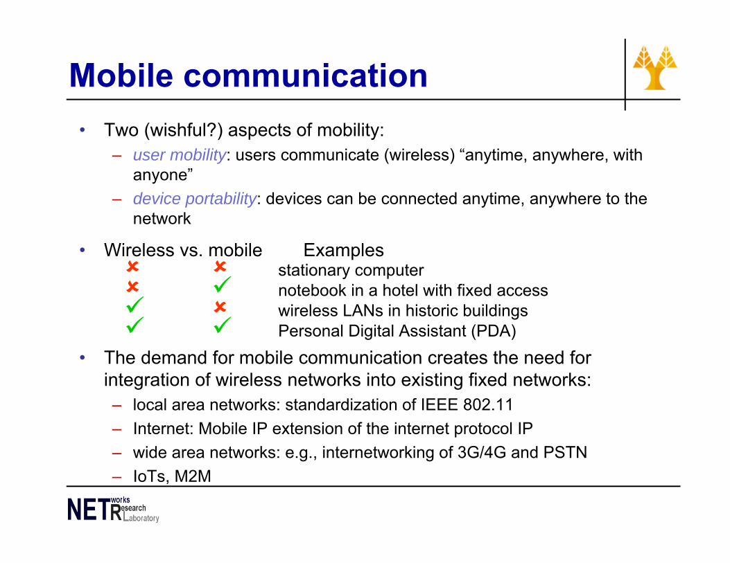
Mobile communication• Two (wishful?) aspects of mobility:

– user mobility: users communicate (wireless) “anytime, anywhere, with anyone”

– device portability: devices can be connected anytime, anywhere to the network

• Wireless vs. mobile Examples stationary computer notebook in a hotel with fixed access wireless LANs in historic buildings Personal Digital Assistant (PDA)

• The demand for mobile communication creates the need for integration of wireless networks into existing fixed networks:– local area networks: standardization of IEEE 802.11– Internet: Mobile IP extension of the internet protocol IP– wide area networks: e.g., internetworking of 3G/4G and PSTN– IoTs, M2M

Challenges for wireless / mobile networks• 2 grand challenges (beyond those for traditional

fixed networks)– Wireless link

• Capacity of link affected by many factors, e.g. (dynamic) spectrum allocation

• Quality of link connection is subjected to many (environmental) factors and can vary substantially

– Mobility• Wireless link quality is adversely affected by device location

(distance) from transmitting / receiving source ( where varies between about 2 to 4)

• Device / node portability

1ad

Effects of device portability• Power consumption

– limited computing power, low quality displays, small disks due to limited battery capacity

– CPU: power consumption ~ CV2f• C: internal capacity, reduced by integration• V: supply voltage, can be reduced to a certain limit• f: clock frequency, can be reduced temporally

• Loss of data– higher probability, has to be included in advance into the design

(e.g., defects, theft)• Limited user interfaces

– compromise between size of fingers and portability– integration of character/voice recognition, abstract symbols

• Limited memory– limited value of mass memories with moving parts– flash-memory or ? as alternative

Challenges in wireless / mobile communication• Wireless Communication

– transmission quality (bandwidth, error rate, delay)– modulation, coding, interference– media access, regulations– ...

• Mobility– location dependent services– location transparency– quality of service support (delay, jitter, security)– ...

• Portability– power consumption– limited computing power, sizes of display, ...– usability– ...

• Addressability (especially for Internet connected devices) and security– Internet addresses are linked to the Network Point of Attachment (NPA) which has physical

meaning– In sensor networks a different meaning of addressing

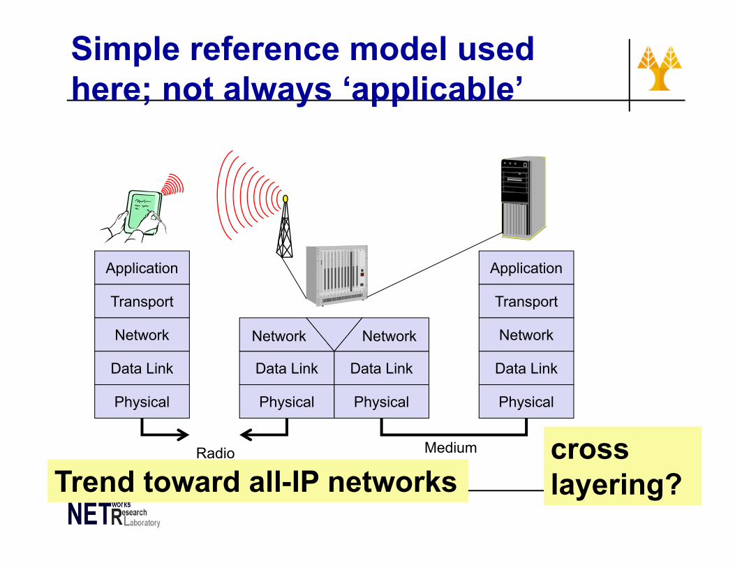
Simple reference model used here; not always ‘applicable’

Application

Transport

Network

Data Link

Physical

Medium

Data Link

Physical

Application

Transport

Network

Data Link

Physical

Data Link

Physical

Network Network

Radio

Trend toward all-IP networkscross layering?

Influence of mobile communication to the layer model

– service location– new applications, multimedia– adaptive applications– congestion and flow control– quality of service– addressing, routing,

device location– hand-over– authentication– media access– multiplexing– media access control– encryption– modulation– interference– attenuation– frequency

• Application layer

• Transport layer

• Network layer

• Data link layer

• Physical layer

The wireless environment

13

Frequencies for communication

VLF = Very Low Frequency UHF = Ultra High FrequencyLF = Low Frequency SHF = Super High FrequencyMF = Medium Frequency EHF = Extra High FrequencyHF = High Frequency UV = Ultraviolet LightVHF = Very High Frequency

Frequency and wave length:λ = c/f wave length λ, frequency fspeed of light c ≅ 3x108m/s,

14

Some frequencies are strictly controlled (pre-assigned by regulating bodies), others are open to use (even by different applications), subject to some given constraints, e.g. Max. Transmit Power

λ f

Frequencies for mobile communication

• VHF-/UHF-ranges for mobile radio simple, small antenna for cars deterministic propagation characteristics, reliable connections

• SHF and higher for directed radio links, satellite communication small antenna, focusing large bandwidth available

• Wireless LANs use frequencies in UHF to SHF spectrum smaller antenna some systems planned up to EHF limitations due to absorption by water and oxygen molecules (resonance frequencies)

15

‘optimum’ antenna size can be related to λ (λ/2 or similar for optimum power transfer)

Recall: Signals• physical representation of data

– function of time and location• signal parameters: parameters representing the value of

data• classification

continuous time/discrete time continuous values/discrete values analog signal = continuous time and continuous values digital signal = discrete time and discrete values

• Signal parameters of periodic signals: period T, frequency f=1/T, amplitude A, phase shift ϕ sine wave as special periodic signal for a carrier:

s(t) = At sin(2 π ft t + ϕt)

16

Transmitted signal <> received signal!

• Wireless transmission distorts any transmitted signal– Received <> transmitted signal; results in uncertainty at receiver

about which bit sequence originally caused the transmitted signal– Abstraction: Wireless channel describes these distortion effects

• Sources of distortion– Attenuation – energy is distributed to larger areas with increasing distance– Reflection/refraction – bounce of a surface; enter material– Absorption – energy is absorbed without any reflection– Diffraction – start “new wave” from a sharp edge– Scattering – multiple reflections at rough surfaces– Doppler fading – shift in frequencies (loss of center)

17

Example wireless signal strength in a multi-path environment

• Brighter color = stronger signal• Obviously, simple (quadratic)

free space attenuation formula is not sufficient to capture these effects

18

© Jochen Schiller, FU Berlin

Source / access point

Distortion effects: Non-line-of-sight paths• Because of reflection, scattering, …, radio communication is not

limited to direct line of sight communication (good or bad?)– Effects depend strongly on frequency, thus different behavior at higher

frequencies

• Different paths have different lengths = propagation time– Results in delay spread of the wireless channel– Closely related to frequency-selective fading

properties of the channel– With movement: fast fading

19

Line-of-sight path

Non-line-of-sight path

signal at receiver

LOS pulsesmultipathpulses

© Jochen Schiller, FU Berlin

Gain, Attenuation and path loss

20

Attenuation results in path loss• Effect of attenuation: received signal strength is a function of the

distance d between sender and transmitter• Captured by Friis free-space equation

– Describes signal strength at distance d relative to some reference distance d0 < d for which strength is known

– d0 is far-field distance, depends on antenna technology

21

Power received is inversely proportional to distance (free space)

Suitability of different frequencies –Attenuation

• Attenuation depends on the used frequency

• Can result in a frequency-selective channel

– If bandwidth spans frequency ranges with different attenuation properties

22

© http://w

ww.itnu.de/radargrundlagen/grundlagen/gl24-de.htm

l© http://141.84.50.121/iggf/Multimedia/Klimatologie/physik_arbeit.htm

Generalizing the attenuation formula• To take into account stronger attenuation than only

caused by distance (e.g., walls, …), use a larger exponent > 2– is the path-loss exponent

– Rewrite in logarithmic form (in dB):

• Take obstacles into account by a random variation– Add a Gaussian random variable with 0 mean, variance 2 to dB

representation– Equivalent to multiplying with a lognormal distributed r.v. in metric

units ! lognormal fading

23

Range and coverage

See tutorial

24

•range “maximum distance at which two radios can operate and maintain a connection.”

•can use simple geometry to determine the coverage area of an Access Point using the formula to determine the area of a circle (π)r2 where the radius (r) is the range of the Wi-Fi signal.

•The coverage area of an Access Point is often referred to as a cell and these terms are usually used interchangeably.

Link formulas

25

Range Basics• Function of data rate (tradeoff) – the higher the data

rate, the shorter the range.• determining the range of an Access Point,

– a few terms need to be defined and a basic understanding of the mathematics that goes into determining the distance by which a radio signal will travel needs to be provided.

• In an open environment, or what is referred to as Free Space, Power varies inversely with the square of the distance between two points (the receiver and the transmitter). – The stronger the Transmit Power, the higher the signal strength or

Amplitude. Antenna Gain also increases Amplitude and will be further discussed.

• While Gain and Power increase the distance a wireless signal can travel, the expected signal loss (Path Loss) between the transmitter and a receiver reduces it.

26

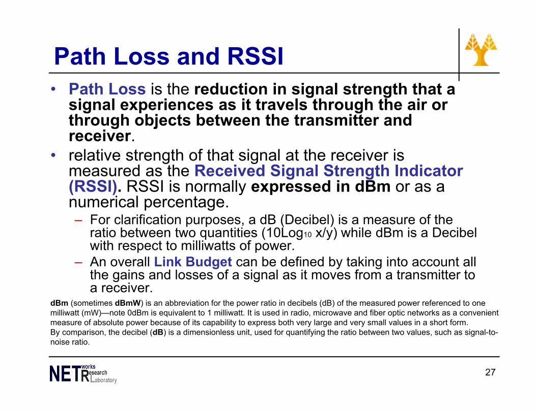
Path Loss and RSSI• Path Loss is the reduction in signal strength that a

signal experiences as it travels through the air or through objects between the transmitter and receiver.

• relative strength of that signal at the receiver is measured as the Received Signal Strength Indicator (RSSI). RSSI is normally expressed in dBm or as a numerical percentage. – For clarification purposes, a dB (Decibel) is a measure of the

ratio between two quantities (10Log10 x/y) while dBm is a Decibel with respect to milliwatts of power.

– An overall Link Budget can be defined by taking into account all the gains and losses of a signal as it moves from a transmitter to a receiver.

27

dBm (sometimes dBmW) is an abbreviation for the power ratio in decibels (dB) of the measured power referenced to one milliwatt (mW)—note 0dBm is equivalent to 1 milliwatt. It is used in radio, microwave and fiber optic networks as a convenient measure of absolute power because of its capability to express both very large and very small values in a short form. By comparison, the decibel (dB) is a dimensionless unit, used for quantifying the ratio between two values, such as signal-to-noise ratio.

• Zero dBm equals one milliwatt. • A 3 dB increase represents roughly doubling the power,

which means that 3 dBm equals roughly 2 mW. For a 3 dB decrease, the power is reduced by about one half, making 3 dBm equal to about 0.5 milliwatt. To express an arbitrary power P as x dBm, or go in the other direction, the following equations may be used:

• or, where P is the power in W and x is the power ratio in dBm.

dBm

28

http://en.wikipedia.org/wiki/DBm

29

dBm level Power Notes

80 dBm 100 kW Typical transmission power of FM radiostation with 50 km range

60 dBm 1 kW = 1000 WTypical combined radiated RF power of microwave oven elements Maximum allowed output RF power from a ham radiotransceiver (rig) without special permissions

50 dBm 100 WTypical thermal radiation emitted by a human body Typical maximum output RF power from a ham radio transceiver (rig)

40 dBm 10 W Typical PLC (Power Line Carrier) Transmit Power

37 dBm 5 W Typical maximum output RF power from a hand held ham radio transceiver (rig)

36 dBm 4 WTypical maximum output power for a Citizens' band radio station (27 MHz) in many countries

33 dBm 2 WMaximum output from a UMTS/3G mobile phone (Power class 1 mobiles) Maximum output from a GSM850/900 mobile phone

30 dBm 1 W = 1000 mWTypical RF leakage from a microwave oven - Maximum output power for DCS 1800 MHz mobile phone Maximum output from a GSM1800/1900 mobile phone

27 dBm 500 mWTypical cellular phone transmission power Maximum output from a UMTS/3G mobile phone (Power class 2 mobiles)

26 dBm 400 mW Access point for Wireless networking

http://en.wikipedia.org/wiki/DBm

Below is a table summarizing useful cases:

30

24 dBm 250 mW Maximum output from a UMTS/3G mobile phone (Power class 3 mobiles)

23 dBm 200 mW Maximum output in interior environment from a WiFi 2.4Ghz antenna (802.11b/g/n).

22 dBm 160 mW

21 dBm 125 mW Maximum output from a UMTS/3G mobile phone (Power class 4 mobiles)

20 dBm 100 mW

Bluetooth Class 1 radio, 100 m range Maximum output power from unlicensed AM transmitter per U.S. Federal Communications Commission (FCC) rules 15.219 [1]. Typical wireless routertransmission power.

15 dBm, 10 dBm, 6 dBm, 5 dBm, 4 dBm 32 mW, 10 mW, 4.0 mW,3.2 mW, 2.5 mW Typical WiFi transmission power in laptops.

3 dBm 2.0 mW Bluetooth Class 2 radio, 10 m range

More precisely (to 8 decimal places) 1.9952623 mW

http://en.wikipedia.org/wiki/DBm

31

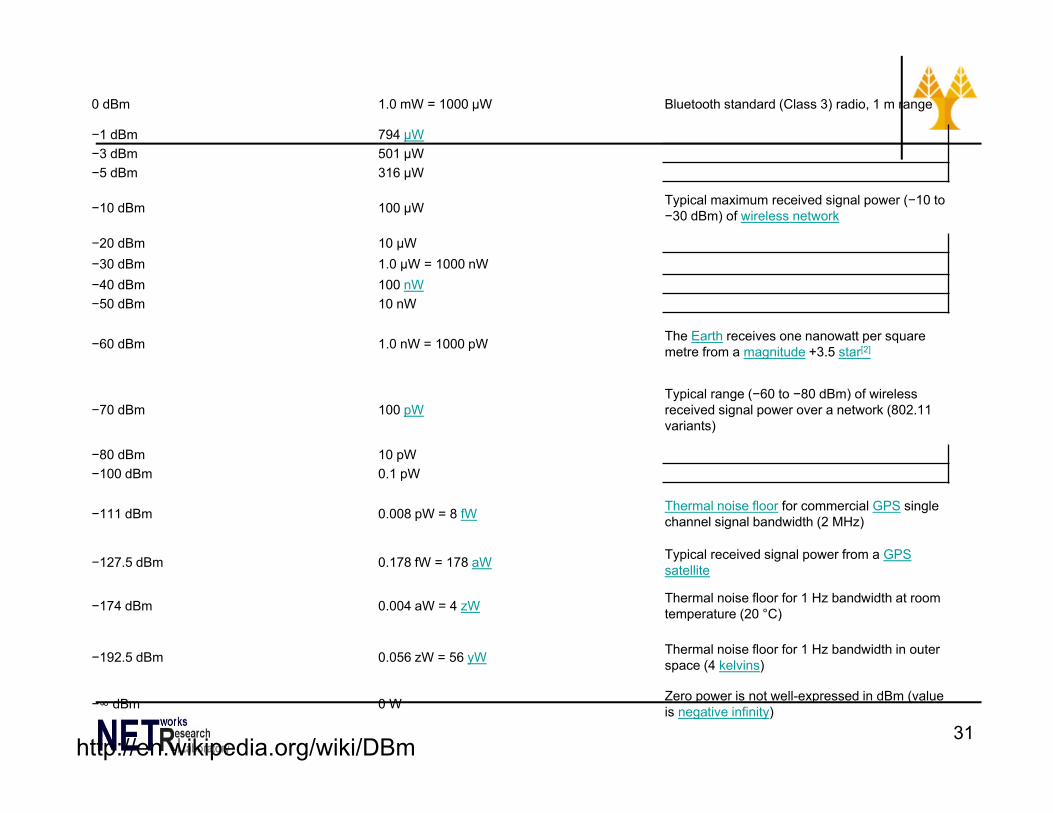
0 dBm 1.0 mW = 1000 µW Bluetooth standard (Class 3) radio, 1 m range

−1 dBm 794 µW−3 dBm 501 µW−5 dBm 316 µW

−10 dBm 100 µW Typical maximum received signal power (−10 to −30 dBm) of wireless network

−20 dBm 10 µW−30 dBm 1.0 µW = 1000 nW−40 dBm 100 nW−50 dBm 10 nW

−60 dBm 1.0 nW = 1000 pW The Earth receives one nanowatt per square metre from a magnitude +3.5 star[2]

−70 dBm 100 pWTypical range (−60 to −80 dBm) of wireless received signal power over a network (802.11 variants)

−80 dBm 10 pW−100 dBm 0.1 pW

−111 dBm 0.008 pW = 8 fW Thermal noise floor for commercial GPS single channel signal bandwidth (2 MHz)

−127.5 dBm 0.178 fW = 178 aW Typical received signal power from a GPS satellite

−174 dBm 0.004 aW = 4 zW Thermal noise floor for 1 Hz bandwidth at room temperature (20 °C)

−192.5 dBm 0.056 zW = 56 yW Thermal noise floor for 1 Hz bandwidth in outer space (4 kelvins)

−∞ dBm 0 W Zero power is not well-expressed in dBm (value is negative infinity)

http://en.wikipedia.org/wiki/DBm

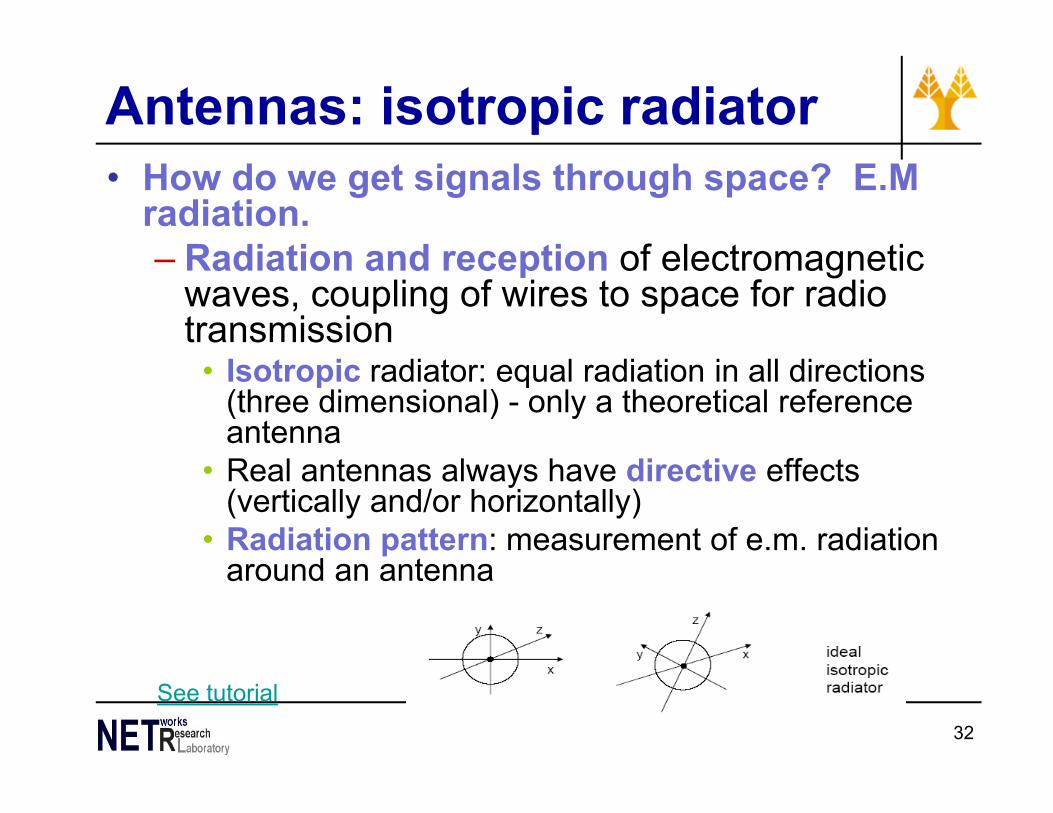
Antennas: isotropic radiator• How do we get signals through space? E.M

radiation.– Radiation and reception of electromagnetic

waves, coupling of wires to space for radio transmission

• Isotropic radiator: equal radiation in all directions (three dimensional) - only a theoretical reference antenna

• Real antennas always have directive effects (vertically and/or horizontally)

• Radiation pattern: measurement of e.m. radiation around an antenna

32

See tutorial

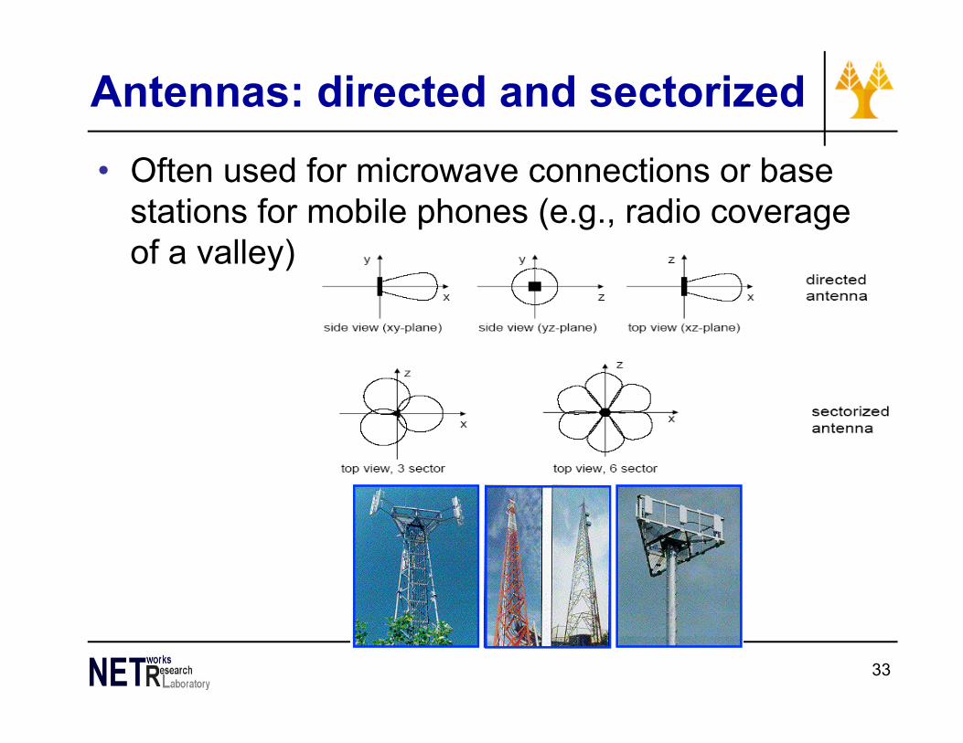
Antennas: directed and sectorized• Often used for microwave connections or base

stations for mobile phones (e.g., radio coverage of a valley)

33

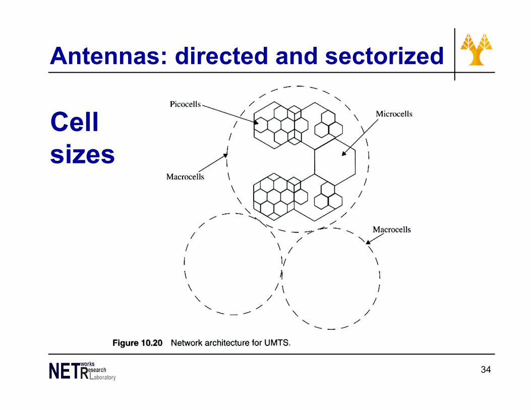
Antennas: directed and sectorized

34

Cell sizes

Antenna gain• Antenna Gain (also known as Amplification) improves range of an

antenna – extends range of a Wi-Fi network. – Gain refers to an increase of the Amplitude or Signal Strength

• One of the advantages of a directional antenna (e.g. a dipole) is greater antenna Gain; this is a result of the RF energy pattern being focused vs. an isotropic design. Other types of antennas are more directional in design taking their radiated energy and squeezing it into a very narrow pattern.

– good analogy: think of the isotropic antenna like a light bulb radiating energy equally in all directions, and the directional antenna like a flash light with the light focused in one direction

– the energy of the directional antenna is concentrated in a particular direction, enabling the beam to travel much farther than an isotropic antenna.

• Antenna Gain is bi-directional so it will amplify the signal as it is being transmitted and as it is received. So if a directional antenna is providing 6db Gain on transmit, it will also increase received sensitivity an equal amount, so the – antenna design of the Wi-Fi Access Point plays a critical role in the

amount of range (coverage) delivered.

35

Antenna gain basics

36

dBidB(isotropic) – the forward gain of an antenna compared with the hypothetical isotropic antenna, which uniformly distributes energy in all directions. Linear polarization of the EM field is assumed unless noted otherwise.

dBddB(dipole) – the forward gain of an antenna compared with a half-wave dipole antenna. 0 dBd = 2.15 dBi

Attenuation

37

RF signal strength is reduced as it passes through various materials. This effect is referred to as Attenuation.

As more Attenuation is applied to a signal, its effective range will be reduced. The amount of Attenuation will vary greatly based on the composition of the material the RF signal is passing through.

Note: A change in power ratio by a factor of two is approximately a 3 dB change20dB is a factor of 100

EIRP• EIRP - Effective Isotropic Radiated Power

EIRP = Power out (dBm) + antenna gain (dBi) – cable loss (dB)

• EIRP Regulations

38

Simplistic Range Calculations

• The Model

For indoor environment the signal power at the receiver SRx is related to the transmit power TRx as shown below (this model can be used as the

reference analysis model)

Where C=speed of light, f=center frequency, N: path loss coefficient. ITU recommends N=3.1 for 5-GHz and N=3 for 2.4-GHz

• IEEE 802.11b (with N=3)• With EIRP of 30dBm max range=154m• With EIRP of 19dBm max range=66.4m• With EIRP of 15dBm max range=48.4m

• IEEE 802.11a (with N=3.1)• With EIRP of 18dBm range=14m with 54Mbits /s• With EIRP of 23dBm range=30m with 54Mbits/s

Simplistic Range Calculations

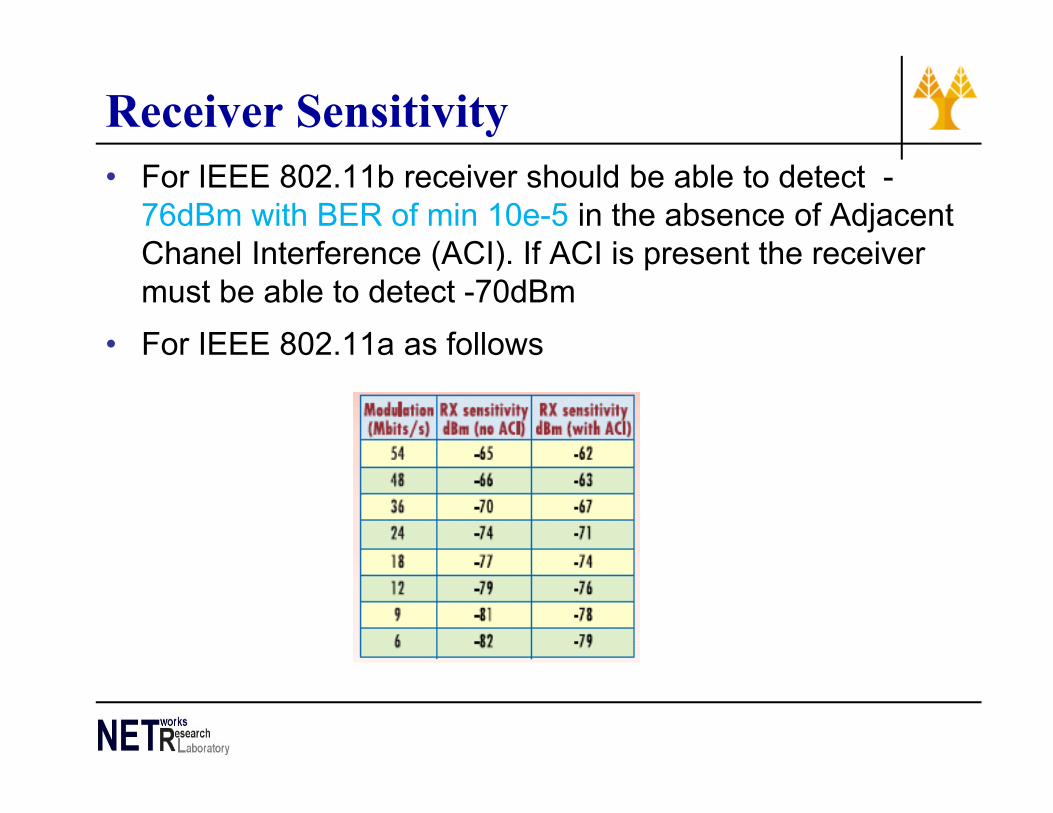
Receiver Sensitivity• For IEEE 802.11b receiver should be able to detect -

76dBm with BER of min 10e-5 in the absence of Adjacent Chanel Interference (ACI). If ACI is present the receiver must be able to detect -70dBm

• For IEEE 802.11a as follows

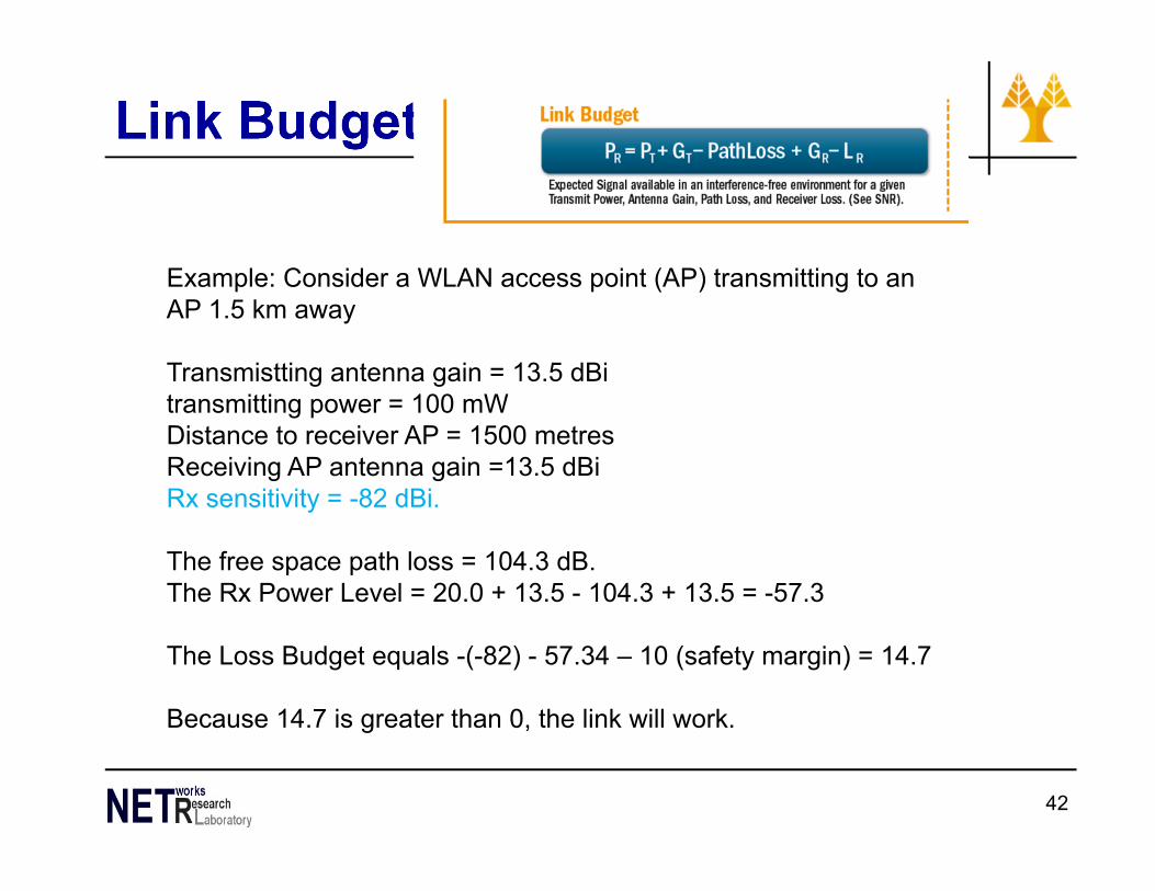
Link Budget

42

Example: Consider a WLAN access point (AP) transmitting to an AP 1.5 km away

Transmistting antenna gain = 13.5 dBi transmitting power = 100 mW Distance to receiver AP = 1500 metres Receiving AP antenna gain =13.5 dBi Rx sensitivity = -82 dBi.

The free space path loss = 104.3 dB.The Rx Power Level = 20.0 + 13.5 - 104.3 + 13.5 = -57.3

The Loss Budget equals -(-82) - 57.34 – 10 (safety margin) = 14.7

Because 14.7 is greater than 0, the link will work.

Signals in noise and interference

43

Signal-to-Noise Ratio (SNR)• The range of an Access Point is a function of data rate.

– notion that higher data rates do not appear to “travel” as far as the lower data rates is a function of the Signal to Noise Ratio (SNR) and not because the Access Point and the client can’t necessarily “hear” each other.

• SNR is the ratio of the desired signal to that of all other noise and interference as seen by a receiver. SNR is important as it determines which data rates can be correctly decoded in a wireless link.

• It is expressed in dB as a ratio.– The received signal and the noise level, determine the SNR. – As data rates increase from 6 Mbps to 54 Mbps, more complex

modulation and encoding methods are used that require a higher SNR to properly decode the signal.

• E.g. a 54 Mbps per second signal requires 25 db of SNR: signal will not be properly decoded at greater distances because as the signal moves further from the source, a greater amount of path loss occurs (the signal is attenuated). Lower data rate transmissions, can be more easily decoded and as a result appear to “travel” farther.

• E.g. in an outdoor environment with just free space loss, a 6 Mbps signal can actually be decoded 7 times further away than a 54 Mbps.

44

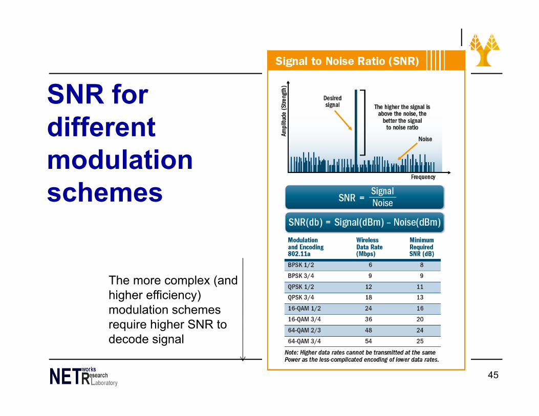
SNR for different modulation schemes

45

The more complex (and higher efficiency) modulation schemes require higher SNR to decode signal

Noise and interference• So far: only a single transmitter assumed

– Only disturbance: self-interference of a signal with multi-path “copies” of itself

• In reality, two further disturbances– Noise – due to effects in receiver electronics, depends on

temperature• Typical model: an additive Gaussian variable, mean 0, no correlation

in time – Interference from third parties

• Co-channel interference: another sender uses the same spectrum• Adjacent-channel interference: another sender uses some other

part of the radio spectrum, but receiver filters not good enough to fully suppress it

• Effect: Received signal is distorted by channel, corrupted by noise and interference– What is the result on the received bits?

46

Symbols and bit errors• Extracting symbols out of a distorted/corrupted wave

form is fraught with errors– Depends essentially on strength of the received signal compared

to the corruption – Captured by signal to noise and interference ratio (SINR)

• SINR allows to compute bit error rate (BER) for a given modulation– Also depends on data rate R (# bits/symbol) of modulation – E.g., for simple DPSK, data rate corresponding to bandwidth:

47

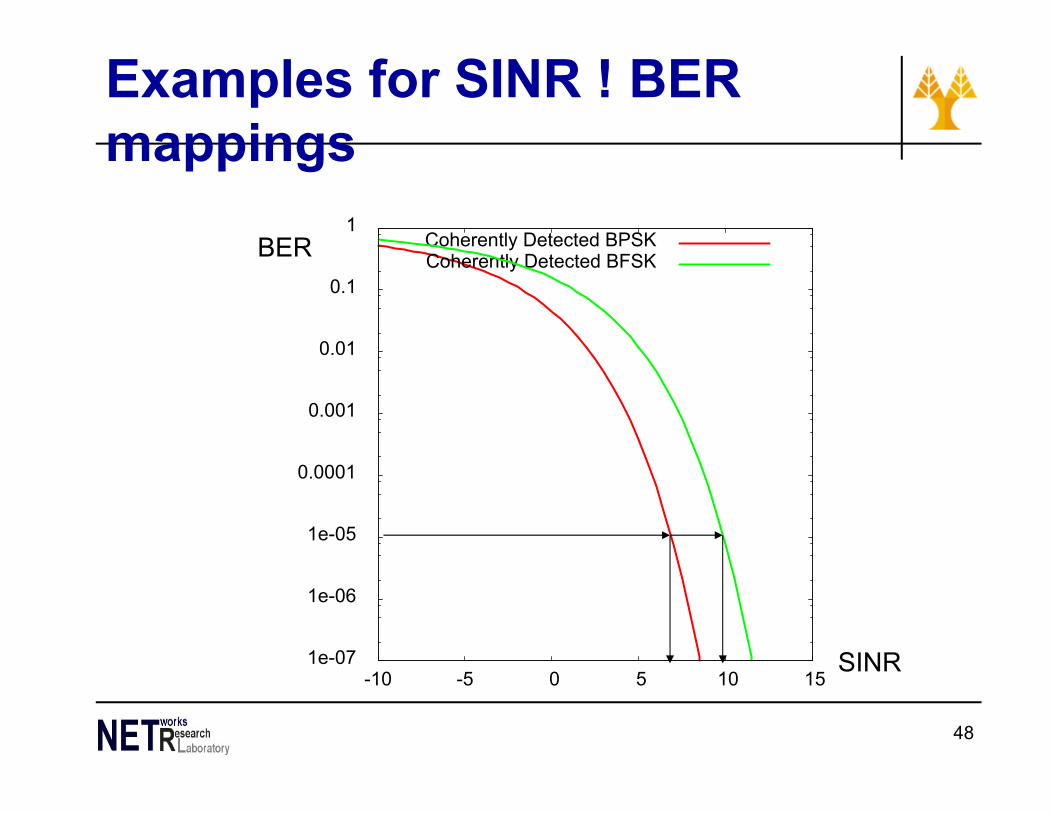
Examples for SINR ! BER mappings

48

1e-07

1e-06

1e-05

0.0001

0.001

0.01

0.1

1

-10 -5 0 5 10 15

Coherently Detected BPSKCoherently Detected BFSKBER

SINR

Signal Important quantities • Important quantities to measure the strength of the signal to the

receiver, noise, interference e.g. SNR . Signal to Noise Ratio in dB SIR = Signal to Interference Ratio; received power of reference user

in dBm/received power of all interferers in dBm C/I . Carrier over Interference in dB

Carrier Power (dBm) / received power of all interferers in dBm

49

Signal Important quantities -Examples• SNR – Signal to Noise Ratio

Assumptions to simplify things:- All the users are equally distributed in the coverage area so that they have equal

distances to the TRX Antenna- The power level they use is the same thus the interference they cause is on the same

level.- All the UEs use the same Baseband rate e.g. 60 kbits/sec for Streaming Video.

If assumed that there are X users under the same TRX Coverage (in the same Cell) and the above assumptions are applied, it means that there are X – 1 users causing interference to one (1) user. This indicates the Signal to Noise Ratio and when expressed in mathematical format the outcome is the following equation:

Where P is the power required for information transfer in one channel and is a multiple of the energy used per bit (Eb) and the Baseband rate ( P = Eb x Baseband rate)

)1(

XPPSNR

50

Bit Error Rate• IEEE 802.11b for BER better than 10e-5 then min S/N

• IEEE 802.11a for BER better than 10e-5 then min S/N

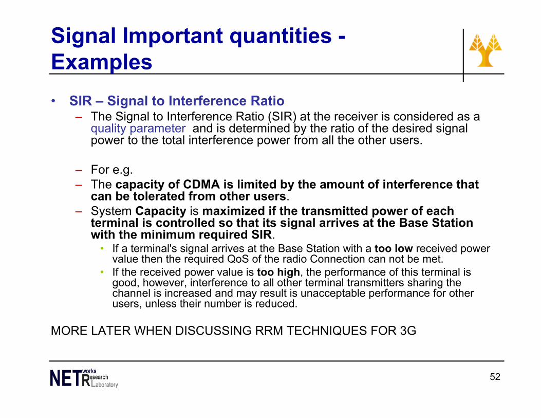
Signal Important quantities -Examples• SIR – Signal to Interference Ratio

– The Signal to Interference Ratio (SIR) at the receiver is considered as a quality parameter and is determined by the ratio of the desired signal power to the total interference power from all the other users.

– For e.g.– The capacity of CDMA is limited by the amount of interference that

can be tolerated from other users.– System Capacity is maximized if the transmitted power of each

terminal is controlled so that its signal arrives at the Base Station with the minimum required SIR.

• If a terminal's signal arrives at the Base Station with a too low received power value then the required QoS of the radio Connection can not be met.

• If the received power value is too high, the performance of this terminal is good, however, interference to all other terminal transmitters sharing the channel is increased and may result is unacceptable performance for other users, unless their number is reduced.

MORE LATER WHEN DISCUSSING RRM TECHNIQUES FOR 3G

52

Signal Important quantities -Examples• C/I – Carrier to Interference Ratio

The Wideband Signal to Interference (SIR) Ratio is also called as Carrier to Interference Ratio (C/I). The Carrier to Interference (C/I) Ratio is very important in Cellular systems in order to determine the maximum allowed interference level for which the system will work.

• Eb/No: The Required Eb/No (measured in dB) for a service denotes the value that the signal energy per bit (Eb) divided by the interference and noise power density (No) should have for achieving a certain BER (Bit Error Rate) so as to satisfy the required QoS of a service.

– Eb/No is the measure of signal to noise ratio for a digital communication system. It is measured at the input to the receiver and is used as the basic measure of how strong the signal is.

– it is the fundamental prediction tool for determining a digital link's performance. Another, more easily measured predictor of performance is the carrier-to-noise or C/N ratio

See www.sss-mag.com/ebn0.html

53fb-bit rate, Bw receiver noise bandwidth

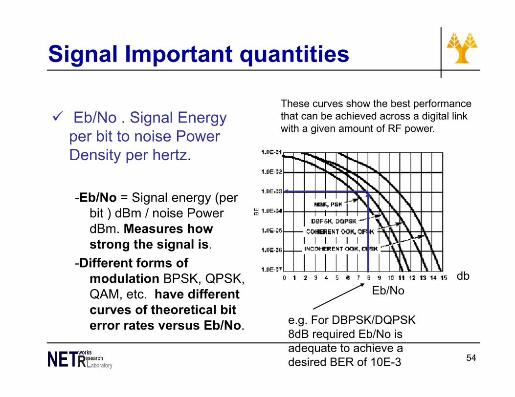
Signal Important quantities

Eb/No . Signal Energy per bit to noise Power Density per hertz.

-Eb/No = Signal energy (per bit ) dBm / noise Power dBm. Measures how strong the signal is.

-Different forms of modulation BPSK, QPSK, QAM, etc. have different curves of theoretical bit error rates versus Eb/No.

54

Eb/No

e.g. For DBPSK/DQPSK 8dB required Eb/No is adequate to achieve a desired BER of 10E-3

db

These curves show the best performance that can be achieved across a digital link with a given amount of RF power.

Example calculation• Consider a 12.2 kbps speech service spread over a 5 MHz

Carrier and that an Eb/No of 5.0 dB is required to achieve a 0.01 BER performance.

– After the dispreading in the receiver, the signal power needs to be typically a few decibels (dB) above the interference and noise power.

– Since an Eb/No of 5.0 dB is enough for efficiently detecting the signal, the required wideband Signal to Interference Ratio (SIR) will be 5.0 dB minus the Processing Gain of 25 dB that can be achieved for the corresponding service (10 x log (WCDMA Chip Rate/Bit Rate)). The chip rate is equal with 3.84 Mcps.

– Thus, the signal power can be 20 dB under the interference and thermal noise power, and the WCDMA receiver can still efficiently detect and interpret the signal correctly.

55

56

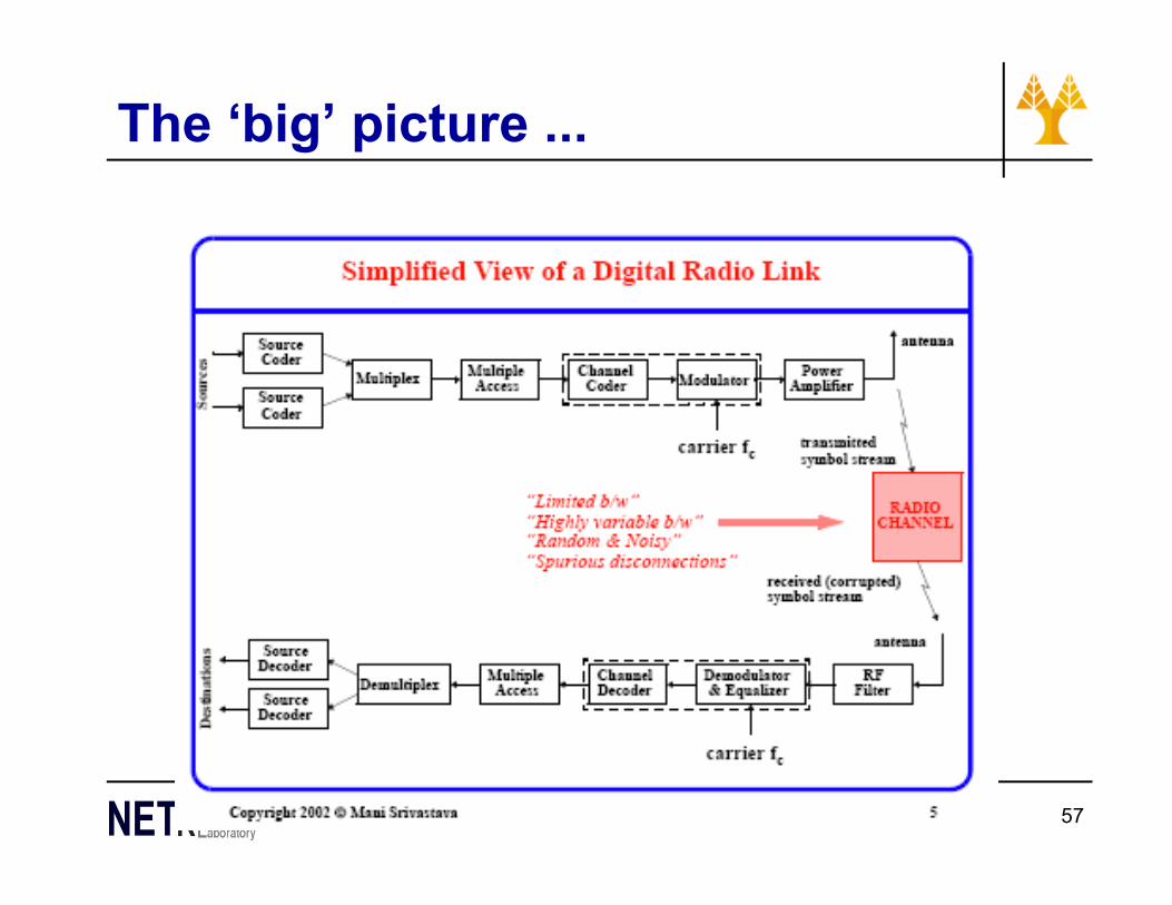
The ‘big’ picture ...

57

Effects of Mobility on channel

58

Effects of mobility on channel

• Channel characteristics change over time and location signal paths change different delay variations of

different signal parts different phases of signal parts

quick changes in the power received (short term fading)

• Additional changes in distance to sender obstacles further away

slow changes in the average power received (long term fading)

59

See mobility models papers for modelling Mobility paper 1, paper 2

Supplementary slides

60

Signal propagation ranges

• Transmission range communication possible low error rate

• Detection range detection of the signal

possible no communication possible

• Interference range signal may not be detected signal adds to the

background noise

61

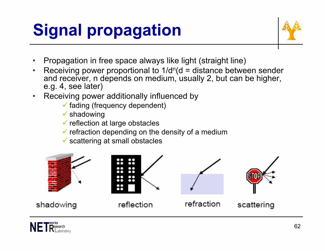
Signal propagation• Propagation in free space always like light (straight line)• Receiving power proportional to 1/dn(d = distance between sender

and receiver, n depends on medium, usually 2, but can be higher, e.g. 4, see later)

• Receiving power additionally influenced by fading (frequency dependent) shadowing reflection at large obstacles refraction depending on the density of a medium scattering at small obstacles diffraction at edges

62

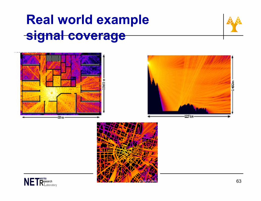
Real world examplesignal coverage

63

Multipath propagation

• Signal can take many different paths between sender and receiver due to reflection, scattering, diffraction

• Time dispersion: signal is dispersed over time interference with “neighbor” symbols, Inter Symbol Interference

(ISI)• The signal reaches a receiver directly and phase shifted

distorted signal depending on the phases of the different parts

64

Typical large-scale path loss

65

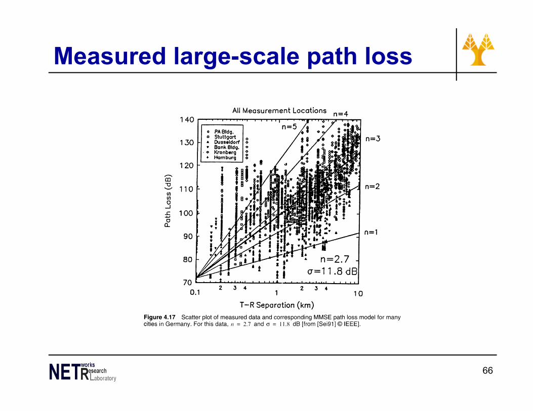
Measured large-scale path loss

66

Partition losses

67

Measured indoor path loss

68

Measured indoor path loss

69

Measured received power levels over a 605 m 38 GHz fixed wireless link in clear sky, rain, and hail [from [Xu00], ©IEEE].

70

Measured received power during rain storm at 38 GHz [from [Xu00], ©IEEE].

71