Dynamic Stiffness of Monopiles Supporting Offshore Wind Turbine Generators Masoud Shadlou 1 , Subhamoy Bhattacharya 1 1 Department of Civil and Environmental Engineering, University of Surrey, GU2 7XH, UK Corresponding author: Professor Subhamoy Bhattacharya Chair in Geomechanics University of Surrey Guildford GU2 7XH Email: [email protected]
Transcript
Dynamic Stiffness of Monopiles Supporting Offshore Wind Turbine Generators
Masoud Shadlou1, Subhamoy Bhattacharya1
1 Department of Civil and Environmental Engineering, University of Surrey, GU2 7XH, UK
Corresponding author:Professor Subhamoy BhattacharyaChair in GeomechanicsUniversity of SurreyGuildfordGU2 7XHEmail: [email protected]
Very large diameter steel tubular piles (up to 10m in diameter, termed as XL or XXL monopiles) and caissons are currently used as foundations to support offshore Wind Turbine Generators (WTG) despite limited guidance in codes of practice. The current codes of practice such as API/DnV suggest methods to analysis long flexible piles which are being used (often without any modification) to analyse large diameter monopiles giving unsatisfactory results. As a result, there is an interest in the analysis of deep foundation for a wide range of length to diameter (L/D) ratio embedded in different types of soil.
This paper carries out a theoretical study utilising Hamiltonian principle to analyse deep foundations (L/D≥2) embedded in three types of ground profiles (homogeneous, inhomogeneous and layered continua) that are of interest to offshore wind turbine industry. Impedance functions (static and dynamic) have been proposed for piles exhibiting rigid and flexible behaviour in all the 3 ground profiles. Through the analysis, it is concluded that the conventional Winkler-based approach (such as p-y curves or Bean-on-Dynamic Winkler Foundations) may not be applicable for piles or caissons having aspect ratio less than about 10 to 15. The results also show that, for the same dimensionless frequency, damping ratio of large diameter rigid piles is higher than long flexible piles and is approximately 1.2 to 1.5 times the material damping. It is also shown that Winkler-based approach developed for flexible piles will under predict stiffness of rigid piles, thereby also under predicting natural frequency of the WTG system. Four wind turbine foundations from four different European wind farms have been considered to gain further useful insights.
1- Background, introduction and a brief literature review
1.1 Challenges in the design of monopiles for offshore wind turbines
Very large diameter steel tubular piles (known as XL or XXL monopiles) and caissons with very low aspect ratio (length-to-diameter) are currently used as foundations to support offshore Wind Turbine Generators (WTG). Around 70% of the world’s offshore WTG foundations are large diameter monopiles (3 - 7m in diameter installed 15 - 40m into the seabed) and accounts for about 20 to 33% of the project costs. The high costs are due to uncertainty in the design (i.e. limited design guidance in codes of practices) as well as fabrication and installation of these relatively new type of foundations. While load and moment carrying capacities (Ultimate Limit State i.e. ULS design which is essentially the moment carrying capacity i.e. strength design) is a necessary condition, the governing design criteria is the SLS (Serviceability Limit State) and FLS (Fatigue Limit State) conditions which requires the estimation of the stiffness of the foundation i.e. pile head stiffness.
Stiffness of the foundation dictates the deformation of the wind turbine tower (which is restricted to 0.5 degrees rotation at the mudline level based on the current DnV code) under operational and extreme loads. Stiffness of the foundation also determines the natural frequency of the whole system which is another design constraint, if not the most challenging aspect of the design process. WTG structures are dynamically sensitive due to the fact that the first natural frequency of these systems (typically 0.25 to 0.35Hz) are very close to the forcing frequencies imposed upon them by the wave, 1P (rotor frequency) and 2P/3P (blade passing frequency). As a result, obtaining natural frequency of the system is an important design calculation. Further details on the challenges in designing foundations for offshore wind turbines can be found in Bhattacharya [1].
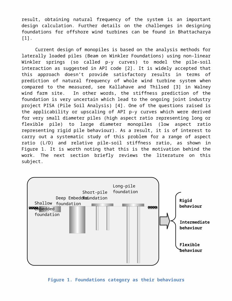
Current design of monopiles is based on the analysis methods for laterally loaded piles (Beam on Winkler Foundations) using non-linear Winkler springs (so called p-y curves) to model the pile-soil interaction as suggested in API code [2]. It is widely accepted that this approach doesn’t provide satisfactory results in terms of prediction of natural frequency of whole wind turbine system when compared to the measured, see Kallahave and Thilsed [3] in Walney wind farm site. In other words, the stiffness prediction of the foundation is very uncertain which lead to the ongoing joint industry project PISA (Pile Soil Analysis) [4]. One of the questions raised is the applicability or upscaling of API p-y curves which were derived for very small diameter piles (high aspect ratio representing long or flexible pile) to large diameter monopiles (low aspect ratio representing rigid pile behaviour). As a result, it is of interest to carry out a systematic study of this problem for a range of aspect ratio (L/D) and relative pile-soil stiffness ratio, as shown in Figure 1. It is worth noting that this is the motivation behind the work. The next section briefly reviews the literature on this subject.
Shallow embedded foundation
Deep Embedded foundation
Short-pile foundationLong-pile foundation
Rigid behaviour
Flexible behaviour
Intermediate behaviour
Figure 1. Foundations category as their behaviours
1.2 A brief literature review on analysis of piles
Using subgrade reaction approach (Beam-on-Winkler Foundation), Hetenyi [5] classified pile foundations as short, intermediate length, and long piles. The boundaries of classification had been refined by Poulos & Davis [6], but keeping the same concept. Adopting the terminology of effective length of laterally loaded pile [7], long-flexible pile was defined as the pile having the length greater than active length (Lac) or effective length (Lc) ( [8], [9]). Carter & Kulhawy [10] extended the previous investigations by proposing three cases of behaviour for pile as: rigid behaviour, intermediate behaviour, and flexible behaviour. Two lengths were presented to differentiate pile behaviour as: (1) rigid length (Lr), and (2) effective length (Lc). The research presented in this paper examines the above concepts in the light of WTG foundations to be applied to a wide range of elastic soils (homogeneous, linear-inhomogeneous and parabolic-inhomogeneous). To generalize the behaviour of the laterally loaded foundations and piles, the concept of classification (as shown in Figure 1) will be used.
Piles or general deep foundations can be categorized as embedded foundation, rigid pile, intermediate-stiff pile, and flexible pile depending on the length-to-diameter (aspect/ slenderness) ratio and the pile-soil relative stiffness ratio. Finite element (FE) and boundary element (BE) methods are capable of analyzing piles numerically considering full 3D nature of the problem. While these three-dimensional (3D) numerical solutions are feasible, they are not commonly used in practice due to their associated costs and time/ expertise required.
Analytical and semi-analytical methods for piles and foundations are not similar, and as a result, they need to be evaluated separately. For example, the response of a massless-rigid-cylindrical-shallow-embedded foundation (L/D≤2) in a layered soil half-space can be analysed by Cone Model ( [11]) Mass-spring-dashpot model ( [12]) and dynamic impedance functions ( [13], [14]) developed by analytical or semi-analytical solutions are other simplified methods
can be used to analyze shallow foundations. For caissons (drilled shafts, [15]) having length-to-diameter aspect ratio 2≤L/D≤6, Varun et al [16] has recently proposed Winkler-spring coefficients for side and base resistances. Similar modelling techniques were also to develop nonlinear Winkler springs for caissons [17]. Another example of the use of nonlinear Winkler springs to analyse monopile foundations supporting the OWTs has recently carried out by Bisoi and Haldar [18]. A limitation of the Winkler-based approach is that each soil spring responds independently of the adjacent ones and ignores the shear transfer between the soil layers. As a result, it may not be strictly valid for a layered stratum with sharp contrast of stiffness. Pile foundations may be evaluated by a number of coupled or uncoupled solutions reported in the literature such as [19], [20], [8], [21], [22], [10], [23], [24], [25], [26].
Non-dimensional solutions for pile foundations as a practical alternative are based on flexibility functions or impedance functions, initially proposed by Barber [27] and subsequently by Reese and Matlock [28] through subgrade reaction approach. These were further developed by Poulos [29] using elastic continuum solutions based on Mindlin solution, Banerjee and Davies [30] using BE (Boundary Element) methods and Randolph [8], using axisymmetric FE model. These solutions represent a simple method for predicting the pile deflection and rotation at ground level (mudline). Poulos [29] and Banerjee and Davies [30] presented static results in terms of pile-flexibility factor (K R=E p I p/Es L
4) and slenderness ratio (L/D). Since the effect of Ep /E s is difficult to be distinguished through K R and effect of slenderness ratio (L/D) is also difficult to be readily visualized ( [31]), Randolph [8] presented a more effective representation for flexible piles where the flexibility functions are expressed as a function of Ep /E s. Subsequently, Carter and Kulhawy [10] updated Randolph’s representation for rigid piles where the flexibility functions are mainly affected by slenderness ratio. In another development, Gazetas and his co-workers ( [32], [33], [34]) presented the pile-head impedance functions (as an inverse of flexibility matrix) for static and dynamic loading conditions including swaying, rocking and coupled swaying-rocking terms. Non-dimensional and uncoupled solutions are obtained by fitting curves for practical use.
In many cases, elasto-dynamic solutions are also used as an efficient method for calculating the soil and pile responses as an alternative to the sophisticated-numerical solutions (such as FE models), see for example ( [26]) for long-flexible piles. In this study, the method [26] is extended to calculate the response of caissons/piles having slenderness ratio of greater than 2. Impedance functions reported in the literature are also reviewed.
1.3 Aim and scope of the work
Due to the current level of interest in the subject, a generalised theoretical study is conducted to predict the stiffness of deep foundations for a wide range of aspect ratio (L⁄D≥2) embedded in a range of soils (homogeneous, inhomogeneous, and layered continua) under static and dynamic conditions, see Figure 1. Through the analysis, an understanding has been developed on the applicability of p-y curves to short piles exhibiting rigid behaviour. Finally, expressions for stiffness of monopiles have been proposed for three different types of ground profile encountered in practice. These are considered particularly useful as a means to compare with high fidelity numerical analysis. Four wind turbine foundations from four different European wind farms have been considered for discussion.
2- Details of Elasto-dynamic Solution
2.1 Theory and analysis
A single deep foundation embedded in multi-layered soil is modelled by Euler-Bernoulli beam theory. A circular object of radius r0 and length L is surrounded by homogeneous, inhomogeneous, or layered-elastic half-space. Hamilton’s principle for a conservative system states that the integral of the difference between kinetic and potential energies yields to zero variation. For a dynamic system, the interaction is taking to account by mass vibrations, and the following Lagrangian equation may be noted:
1
where, is kinetic energy and is total potential energy including strain energy stored in the system, and is the work done by external loading. It is presumed that there is no separation and slippage at the soil-pile interface. To separate effects of zone of the foundation influence and the soil where the displacement is vanishingly small, two regions are assumed around the pile. Inner region is called near-field region where the soil is influenced by pile motion, and the outer region known as far-field region which is isolated by pile influence.
To solve Lagrangian (Eq. 1), a displacement vector (u=[uruθuz ]T) was used by Shadlou and
Bhattacharya [26], and it was assumed that a fictitious pile is beneath the original pile to model boundary conditions at pile tip level. Above expression is not valid for short and stubby piles or foundations, because:- Foundation behaviour will be influenced by tip resistance - Uniform distribution of soil displacement inside fictitious foundation is not valid for short
foundations.
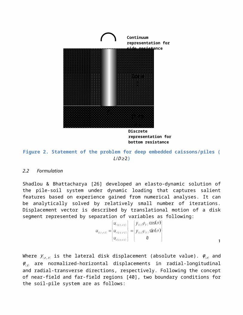
To facilitate the above effects for a deep foundation (exhibiting rigid, relative stiff, or flexible behaviour) under lateral and rocking loading, it is essential to model the foundation tip. This can be done by separating the tip resistance from the side resistance. Modelling surface foundations induced by dynamic loadings and supported on different soil strata was state-of-the-art in late 60s to 80s ( [35]). It is assumed that the resistance of foundation tip is similar to the resistance of rigid surface foundations. Hence foundation tip is modelled by discrete-dynamic impedance functions. As a result, the soil surrounding and beneath the foundation is divided into two zones (Error: Reference source not found).The side of the deep foundation (zone I) is modelled by the continuum approach and foundation tip (zone II) is formulated by appropriate dynamic impedance function as reported in the literature. In this case, dynamic impedance functions will be assigned based on the properties of surface foundations.
Veletsos & Verbic [36], and Luco [13] proposed a simple impedance function for surface circular foundations rested on homogeneous-elastic half space. This function can theoretically be expressed as following:
Continuum representation for side resistance
Discrete representation for bottom resistance
Zone I
Zone II
2 where a0=ωr /V s is dimensionless frequency, and r , V s, and ω are foundation radius, shear wave velocity of soil, and rotational frequency of vibration, respectively. Kausel [37], and Kausel & Ushijima [38] proposed dynamic impedance functions for a rigid circular foundation supported on a stratum-over-rigid base. Tasoulas & Kausel [39] further investigated the dynamic impedance function of the circular ring footings on an elastic stratum. For the sake of simplicity, simple formulation presented in Eq. 2 is used for foundation tip resistance. Hence it will additionally be assumed in the current research that the soil beneath the foundation is homogeneous-elastic half-space.
Figure 2. Statement of the problem for deep embedded caissons/piles (L/D≥2)
2.2 Formulation
Shadlou & Bhattacharya [26] developed an elasto-dynamic solution of the pile-soil system under dynamic loading that captures salient features based on experience gained from numerical analyses. It can be analytically solved by relatively small number of iterations. Displacement vector is described by translational motion of a disk segment represented by separation of variables as following:
1
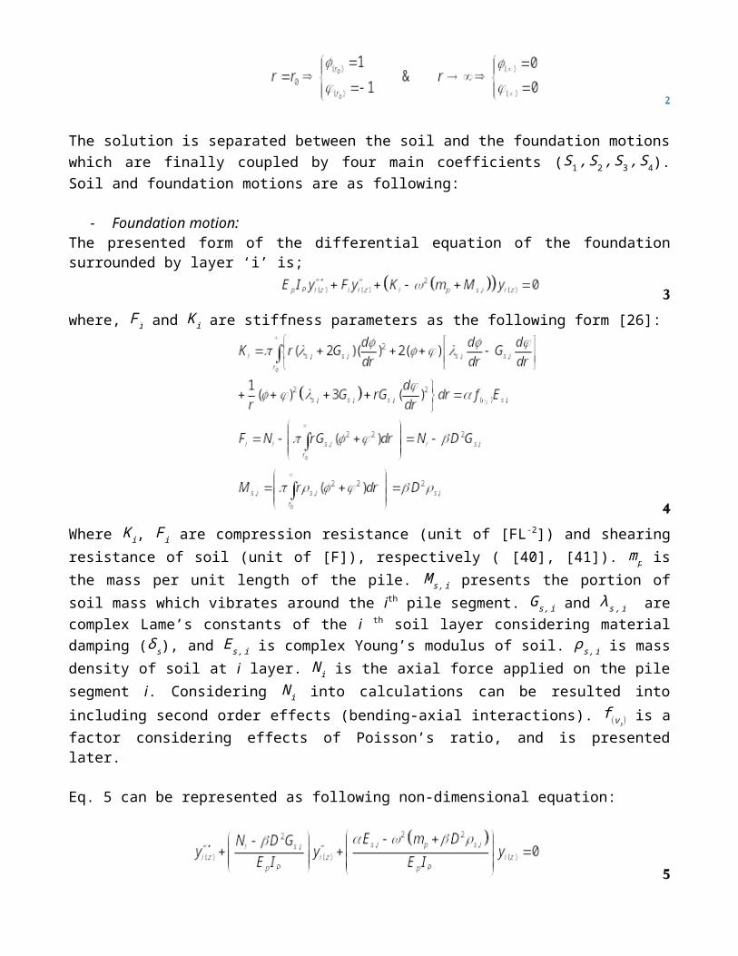
Where y(z ,t ) is the lateral disk displacement (absolute value). ϕ(r) and φ(r) are normalized-horizontal displacements in radial-longitudinal and radial-transverse directions, respectively. Following the concept of near-field and far-field regions [40], two boundary conditions for the soil-pile system are as follows:
2
The solution is separated between the soil and the foundation motions which are finally coupled by four main coefficients (S1 , S2 , S3 , S4). Soil and foundation motions are as following:
- Foundation motion:The presented form of the differential equation of the foundation surrounded by layer ‘i’ is;
3 where, F i and K i are stiffness parameters as the following form [26]:
4Where K i, F i are compression resistance (unit of [FL-2]) and shearing resistance of soil (unit of [F]), respectively ( [40], [41]). m p is the mass per unit length of the pile. M s , i presents the portion of soil mass which vibrates around the ith pile segment. Gs , i and λs ,i are complex Lame’s constants of the i th soil layer considering material damping (δ s), and E s ,i is complex Young’s modulus of soil. ρ s ,i is mass density of soil at i layer. N i is the axial force applied on the pile segment i. Considering N i into calculations can be resulted into including second order effects (bending-axial interactions). f (ν s) is a factor considering effects of Poisson’s ratio, and is presented later.
Eq. 5 can be represented as following non-dimensional equation:
5
Where, α and β are non-dimensional stiffness coefficients (compression and shearing) which can be calculated by Eq. 6. Taking α and β into account, effects of vibrating mass and shearing
resistance of soil can be simply adopted by β , and compression resistance of soil can be linked to the traditional (plane strain) Winkler spring form, α E s, ( [19], [42], [43], [26]). Above differential equation is distinct from the traditional Winkler approach (such as elastic Beam-on-Dynamic-Winkler Foundations and p-y curves) where effects of shearing resistance is ignored. It is worth noting that above equation is also different than two spring models ( [16], [44]) where both rotational and translational springs are positive constants. Rotational and translational springs have different definitions than shearing and compression stiffness. The former has positive rotational spring and the later has negative shearing spring. Therefore their solutions can be separated. On the other hand, the rotational and translational springs are constant independent of soil and pile properties [44].
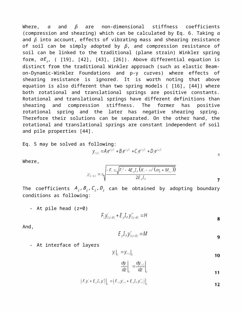
Eq. 5 may be solved as following:
6 Where,
7The coefficients Ai , Bi ,Ci , Di can be obtained by adopting boundary conditions as following:
- At pile head (z=0)
8And,
9 - At interface of layers
10
11
12
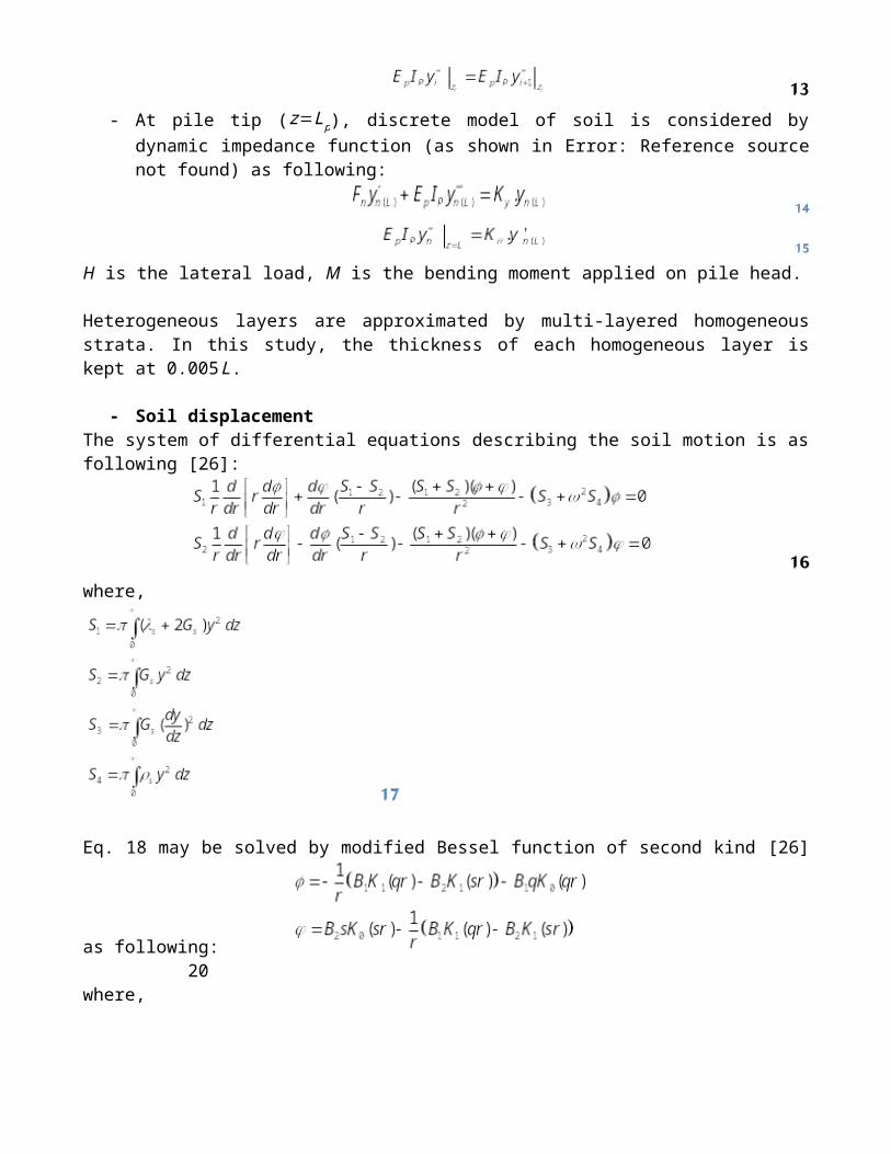
13 - At pile tip (z=Lp), discrete model of soil is considered by dynamic impedance function (as
shown in Error: Reference source not found) as following:
14
15 H is the lateral load, M is the bending moment applied on pile head.
Heterogeneous layers are approximated by multi-layered homogeneous strata. In this study, the thickness of each homogeneous layer is kept at 0.005 L.
- Soil displacementThe system of differential equations describing the soil motion is as following [26]:
16 where,
17
Eq. 18 may be solved by modified Bessel function of second kind [26] as following:
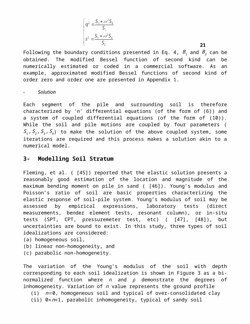
20where,
21Following the boundary conditions presented in Eq. 4, B1 and B2 can be obtained. The modified Bessel function of second kind can be numerically estimated or coded in a commercial software. As an example, approximated modified Bessel functions of second kind of order zero and order one are presented in Appendix 1.
- Solution
Each segment of the pile and surrounding soil is therefore characterized by ‘n’ differential equations (of the form of (6)) and a system of coupled differential equations (of the form of (10)). While the soil and pile motions are coupled by four parameters (S1 , S2 , S3 , S4) to make the solution of the above coupled system, some iterations are required and this process makes a solution akin to a numerical model.
3- Modelling Soil Stratum
Fleming, et al. ( [45]) reported that the elastic solution presents a reasonably good estimation of the location and magnitude of the maximum bending moment on pile in sand ( [46]). Young’s modulus and Poisson’s ratio of soil are basic properties characterizing the elastic response of soil-pile system. Young’s modulus of soil may be assessed by empirical expressions, laboratory tests (direct measurements, bender element tests, resonant column), or in-situ tests (SPT, CPT,
pressuremeter test, etc) ( [47], [48]), but uncertainties are bound to exist. In this study, three types of soil idealizations are considered: (a) homogeneous soil, (b) linear non-homogeneity, and (c) parabolic non-homogeneity.
The variation of the Young’s modulus of the soil with depth corresponding to each soil idealization is shown in Figure 3 as a bi-normalized function where n and ρ demonstrate the degrees of inhomogeneity. Variation of n value represents the ground profile
(i) n=0, homogeneous soil and typical of over-consolidated clay(ii) 0<n<1, parabolic inhomogeneity, typical of sandy soil (iii) n=1, linear inhomogeneity, typical of normally consolidated clay.
On the other hand, ρ defines the Young’s Modulus at the surface as defined in Figure 3. For all the cases, it is assumed that the Poisson’s ratio and mass density of soil are uniform. The depth ( z) and the Young’s modulus of soil at that depth (Es(z)) are normalized by Young’s Modulus of the soil at one diameter depth below (Es(0)). D p is the pile diameter, and H 1is the depth of top layer in layered strata.
Figure 3. Soil idealization as homogeneous, linear inhomogeneous, and parabolic inhomogeneous.
4- Validation
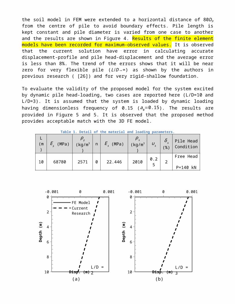
This section compares the results of the analyses to validate the proposed method. The efficiency of the method is investigated with reference to the deformation profile keeping in mind SLS design requirements. A set of time-domain Finite Element analyses has been carried out by 3D FE code in OPENSEES ( [49]) platform for pile foundations in elastic media. For the sake of brevity, only results of system (rigid and flexible piles) embedded in uniform soil stiffness distribution (n=0 , ρ=0) are discussed. First validation is done for the system induced by static head loading. Details of the soil and the pile properties are given in Table 1. The boundaries of the soil model in FEM were extended to a horizontal distance of 80Dp from the centre of pile to avoid boundary
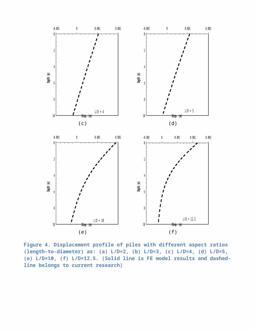
effects. Pile length is kept constant and pile diameter is varied from one case to another and the results are shown in Figure 4. Results of the finite element models have been recorded for maximum-observed values. It is observed that the current solution have error in calculating accurate displacement-profile and pile head-displacement and the average error is less than 8%. The trend of the errors shows that it will be near zero for very flexible pile (L/D→∞) as shown by the authors in previous research ( [26]) and for very rigid-shallow foundation.
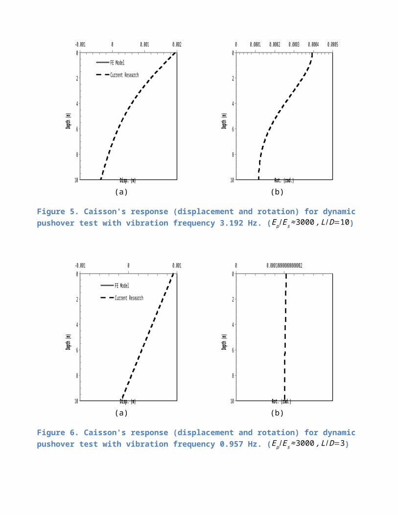
To evaluate the validity of the proposed model for the system excited by dynamic pile head-loading, two cases are reported here (L/D=10 and L/D=3). It is assumed that the system is loaded by dynamic loading having dimensionless frequency of 0.15 (a0=0.15). The results are provided in Figure 5 and 5. It is observed that the proposed method provides acceptable match with the 3D FE model.
Table 1. Detail of the material and loading parameters.L
Figure 4. Displacement profile of piles with different aspect ratios (length-to-diameter) as: (a) L/D=2, (b) L/D=3, (c) L/D=4, (d) L/D=5, (e) L/D=10, (f) L/D=12.5. (Solid line is FE model results and dashed-line belongs to current research)
-0.001 0 0.001 0.0020
2
4
6
8
10
FE Model Current Research
Disp. (m)
Depth (
m)
0 0.0001 0.0002 0.0003 0.0004 0.00050
2
4
6
8
10 Rot. (rad.)
Depth (
m)
(a) (b)
Figure 5. Caisson's response (displacement and rotation) for dynamic pushover test with vibration frequency 3.192 Hz. (Ep /E s≈3000 , L/D=10)
-0.001 0 0.0010
2
4
6
8
10
FE Model Current Research
Disp. (m)
Depth (
m)
0 0.0001000000000000020
2
4
6
8
10 Rot. (rad.)
Depth (
m)
(a) (b)
Figure 6. Caisson's response (displacement and rotation) for dynamic pushover test with vibration frequency 0.957 Hz. (Ep /E s≈3000 , L/D=3)
5- Comparing with methods available in the literature
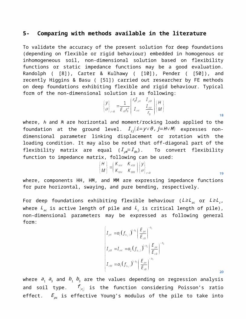
To validate the accuracy of the present solution for deep foundations (depending on flexible or rigid behaviour) embedded in homogenous or inhomogeneous soil, non-dimensional solution based on flexibility functions or static impedance functions may be a good evaluation. Randolph ( [8]), Carter & Kulhawy ( [10]), Pender ( [50]), and recently Higgins & Basu ( [51]) carried out researcher by FE methods on deep foundations exhibiting flexible and rigid behaviour. Typical form of the non-dimensional solution is as following:
18where, H and M are horizontal and moment/rocking loads applied to the foundation at the ground level. I ij(i= y∨θ , j=H∨M ) expresses non-dimensional parameter linking displacement or rotation with the loading condition. It may also be noted that off-diagonal part of the flexibility matrix are equal (I yM=I θH). To convert flexibility function to impedance matrix, following can be used:
19where, components HH, HM, and MM are expressing impedance functions for pure horizontal, swaying, and pure bending, respectively.
For deep foundations exhibiting flexible behaviour (L≥Lac or L≥Lc, where Lac is active length of pile and Lc is critical length of pile), non-dimensional parameters may be expressed as following general form:
20where a1 a3 and b1 b3 are the values depending on regression analysis and soil type. f (νs ) is the function considering Poisson’s ratio effect. Epe is effective Young’s modulus of the pile to take into account solid and hollow pile. Elastic modulus ratio or pile-soil relative stiffness ratio is referred to as Epe /E s from here onwards.
The above equations suggests that the response of foundation exhibiting flexible behaviour is mainly affected by elastic modulus ratio. In order to compare the formulas reported in literature and developed as a part of the current study, the flexibility functions are transformed to impedance functions and are tabulated in Table 2.
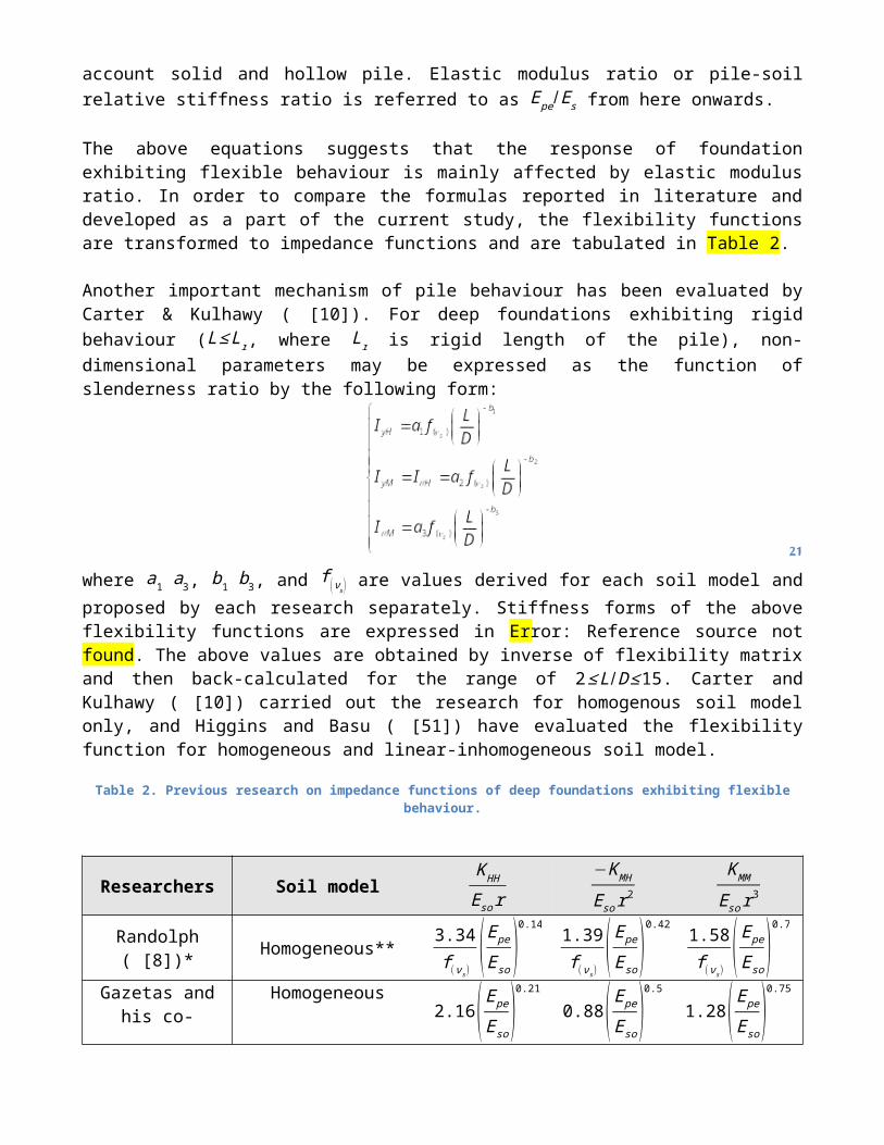
Another important mechanism of pile behaviour has been evaluated by Carter & Kulhawy ( [10]). For deep foundations exhibiting rigid behaviour (L≤Lr, where Lr is rigid length of the pile), non-dimensional parameters may be expressed as the function of slenderness ratio by the following form:
21where a1 a3, b1 b3, and f (νs ) are values derived for each soil model and proposed by each research separately. Stiffness forms of the above flexibility functions are expressed in Error: Referencesource not found. The above values are obtained by inverse of flexibility matrix and then back-calculated for the range of 2≤L/D≤15. Carter and Kulhawy ( [10]) carried out the research for homogenous soil model only, and Higgins and Basu ( [51]) have evaluated the flexibility function for homogeneous and linear-inhomogeneous soil model.
Table 2. Previous research on impedance functions of deep foundations exhibiting flexible behaviour.
Researchers Soil modelK HH
Eso r−KMH
E sor2
KMM
Eso r3
Randolph ( [8])* Homogeneous**3.34f (ν s)
(E pe
E so)
0.14 1.39f (ν s)
( Epe
Eso)
0.42 1.58f (ν s)
( Epe
Eso)
0.7
Gazetas and his co-workers***
Homogeneous 2.16( Epe
Eso)
0.21
0.88( Epe
Eso)
0.5
1.28( Epe
Eso)
0.75
Parabolic inhomogeneous (
n=0.5 , ρ=0)1.58( Epe
Eso)
0.25
0.96( E pe
E so)
0.53
1.2( Epe
E so)
0.77
Linear inhomogeneous (n=1 , ρ=0)
1.2( Epe
E so)
0.28
0.68( Epe
Eso)
0.6
1.12( Epe
E so)
0.8
Pender ( [50])*
Homogeneous 2.57( E pe
Eso)
0.188
1.23( Epe
Eso)
0.47
1.45( Epe
Eso)
0.738
Parabolic inhomogeneous (
n=0.5 , ρ=0)1.7( Epe
Eso)
0.29
0.96( E pe
E so)
0.53
1.2( Epe
E so)
0.77
Linear inhomogeneous (n=1 , ρ=0)
1.47( Epe
Eso)
0.33
1.08( Epe
Eso)
0.55
1.38( Epe
Eso)
0.776
* These data are back-calculated from original flexibility functions proposed by researcher.
** Poisson’s ratio effects may be considered by a function presented by Randolph as f (νs )=1+νs
1+0.75 νs.
*** These results are used in Euro Code 8, part 5, Annex C.
Table 3. Previous research on impedance functions of deep foundations exhibiting rigid behaviour.
Researchers Soil modelK HH
Eso r−KMH
E sor2
KMM
Eso r3
Carter & Kulhawy ( [10])*
Homogeneous**2.7f (νs)
( LD )0.81 3.6
f (νs)( LD )
1.6 14.27f (ν s)
( LD )2.15
Huggins and Basu ( [51])*,***
Homogeneous**4f (νs)
( LD )0.787 5.4
f (νs)( LD )
1.7 14.25f (νs)
( LD )2.47
Linear inhomogeneous** (n=1 , ρ=0)
4f (νs)
( LD )1.66 6.7
f (νs)( LD )
2.6 15.4f (ν s)
( LD )3.45
* These data are back-calculated from original flexibility functions proposed by researcher.
** Poisson’s ratio effects may be considered by a function presented by Randolph as f (νs )=1+νs
1+0.75 νs.
*** it is back-calculated for 2≤L/D≤15
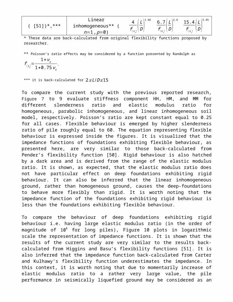
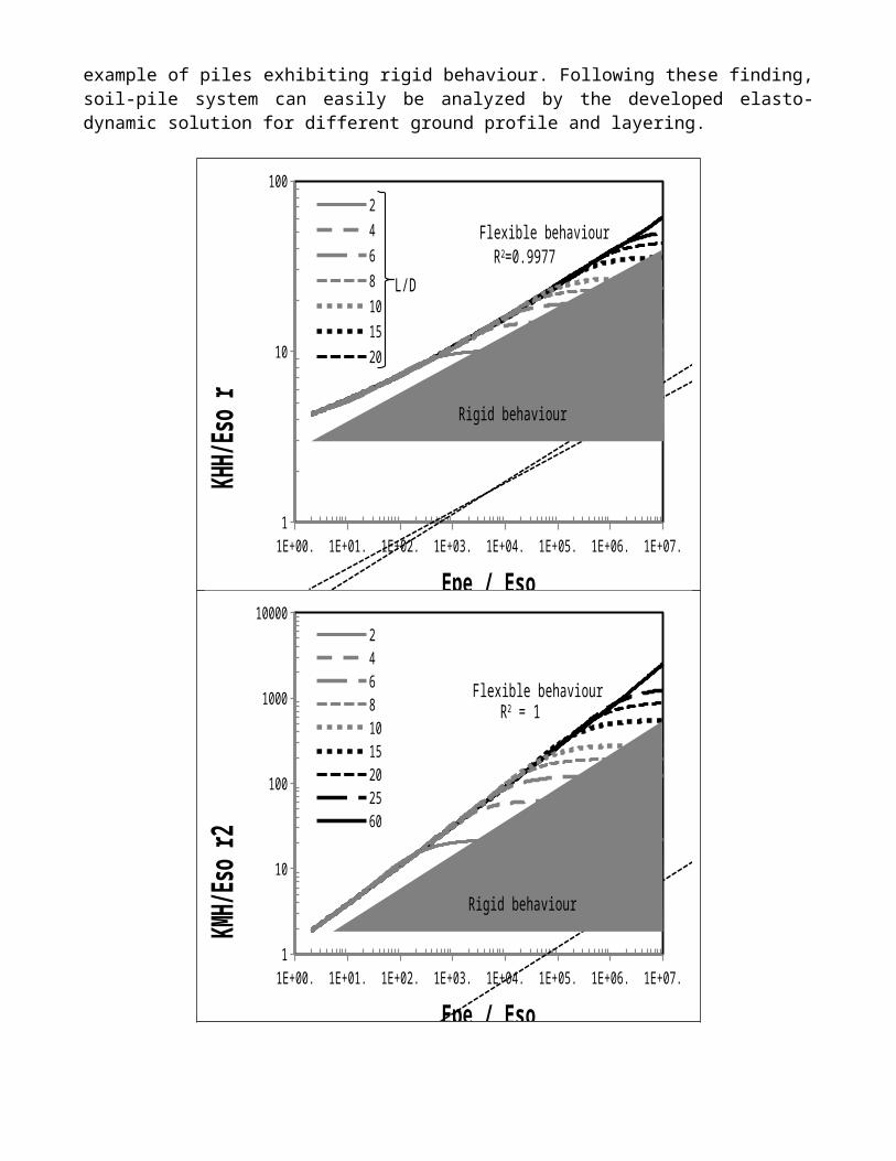
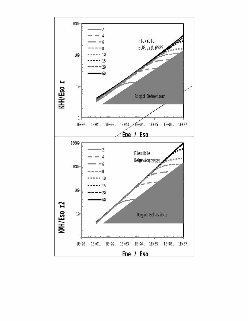
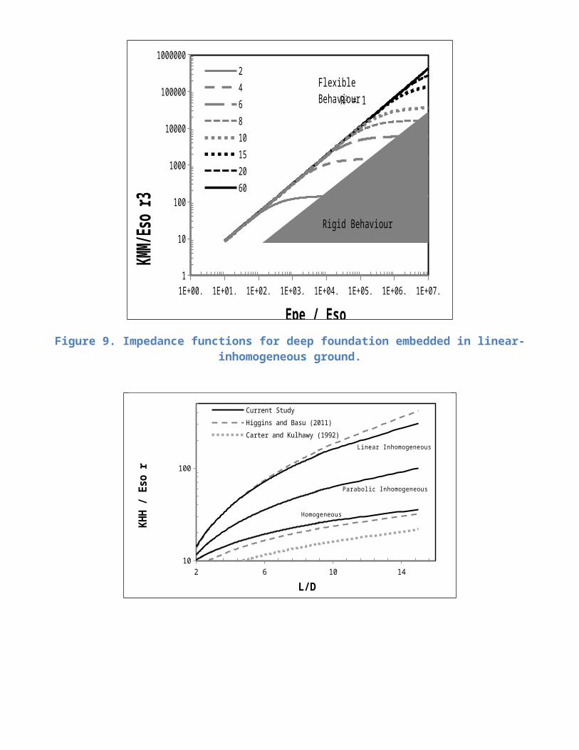
To compare the current study with the previous reported research, Figure 7 to 9 evaluate stiffness component HH, HM, and MM for different slenderness ratio and elastic modulus ratio for homogeneous, parabolic inhomogeneous, and linear inhomogeneous soil model, respectively. Poisson’s ratio are kept constant equal to 0.25 for all cases. Flexible behaviour is emerged by higher slenderness ratio of pile roughly equal to 60. The equation representing flexible behaviour is expressed inside the figures. It is visualized that the impedance functions of foundations exhibiting flexible behaviour, as presented here, are very similar to those back-calculated from Pender’s flexibility function [50]. Rigid behaviour is also hatched by a dark area and is derived from the range of the elastic modulus ratio. It is shown, as expected, that the elastic modulus ratio does not have particular effect on deep foundations exhibiting rigid behaviour. It can also be inferred that the linear inhomogeneous ground, rather than homogeneous ground, causes the deep-foundations to behave more flexibly than rigid. It is worth noting that the impedance function of the foundations exhibiting rigid behaviour is less than the foundations exhibiting flexible behaviour.
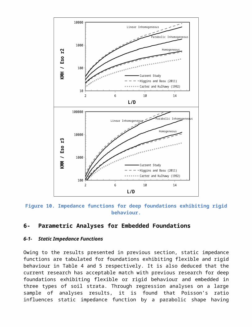
To compare the behaviour of deep foundations exhibiting rigid behaviour i.e. having large elastic modulus ratio (in the order of magnitude of 108 for long piles), Figure 10 plots in logarithmic scale the representation of impedance functions. It is shown that the results of the current study are very similar to the results back-calculated from Higgins and Basu’s flexibility functions [51]. It is also inferred that the impedance function back-calculated from Carter and Kulhawy’s flexibility function underestimates the impedance. In this context, it is worth noting that due to momentarily increase of elastic modulus ratio to a rather very large value, the pile performance in seismically liquefied ground may be considered as an example of piles exhibiting rigid behaviour. Following these finding, soil-pile system can easily be analyzed by the developed elasto-dynamic solution for different ground profile and layering.
Figure 9. Impedance functions for deep foundation embedded in linear-inhomogeneous ground.
2 6 10 1410
100
Current Study
Higgins and Basu (2011)
Carter and Kulhawy (1992)
L/D
KHH
/ Eso
r
Parabolic Inhomogeneous
Homogeneous
Linear Inhomogeneous
2 6 10 1410
100
1000
10000
Current Study
Higgins and Basu (2011)
Carter and Kulhawy (1992)
L/D
KMH
/ Eso
r2
Parabolic Inhomogeneous
Homogeneous
Linear Inhomogeneous
2 6 10 14100
1000
10000
100000
Current Study
Higgins and Basu (2011)
Carter and Kulhawy (1992)
L/D
KMM
/ Es
o r3
Parabolic Inhomogeneous
Homogeneous
Linear Inhomogeneous
Figure 10. Impedance functions for deep foundations exhibiting rigid behaviour.
6- Parametric Analyses for Embedded Foundations
6-1- Static Impedance Functions
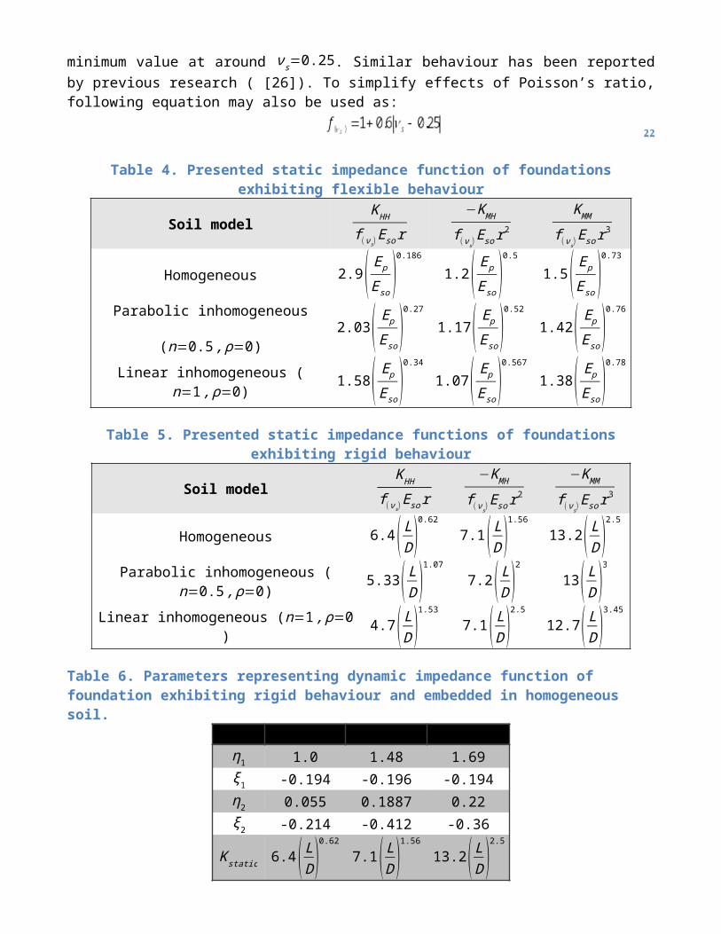
Owing to the results presented in previous section, static impedance functions are tabulated for foundations exhibiting flexible and rigid behaviour in Table 4 and 5 respectively. It is also deduced that the current research has acceptable match with previous research for deep foundations exhibiting flexible or rigid behaviour and embedded in three types of soil strata. Through regression analyses on a large sample of analyses results, it is found that Poisson’s ratio influences static impedance function by a parabolic shape having minimum value at around νs=0.25. Similar behaviour has been reported by previous research ( [26]). To simplify effects of Poisson’s ratio, following equation may also be used as:
22
Table 4. Presented static impedance function of foundations exhibiting flexible behaviour
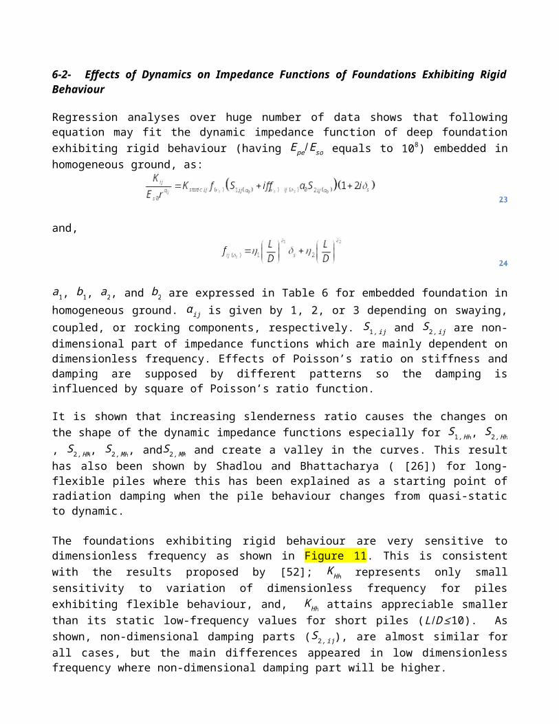
6-2- Effects of Dynamics on Impedance Functions of Foundations Exhibiting Rigid Behaviour
Regression analyses over huge number of data shows that following equation may fit the dynamic impedance function of deep foundation exhibiting rigid behaviour (having Epe /E so equals to 108) embedded in homogeneous ground, as:
23
and,
24
a1, b1, a2, and b2 are expressed in Table 6 for embedded foundation in homogeneous ground. α ij is given by 1, 2, or 3 depending on swaying, coupled, or rocking components, respectively. S1 ,ij and S2 ,ij are non-dimensional part of impedance functions which are mainly dependent on dimensionless frequency. Effects of Poisson’s ratio on stiffness and damping are supposed by different patterns so the damping is influenced by square of Poisson’s ratio function.
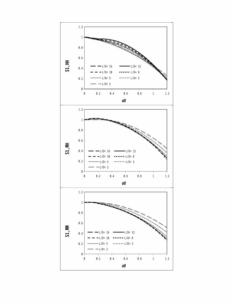
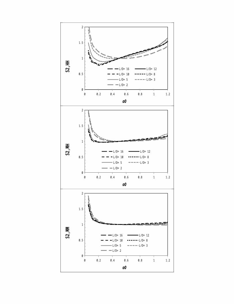
It is shown that increasing slenderness ratio causes the changes on the shape of the dynamic impedance functions especially for S1 , HH , S2 , HH, S2 , HM , S2 , MH, andS2 , MM and create a valley in the curves. This result has also been shown by Shadlou and Bhattacharya ( [26]) for long-flexible piles where this has been explained as a starting point of radiation damping when the pile behaviour changes from quasi-static to dynamic.
The foundations exhibiting rigid behaviour are very sensitive to dimensionless frequency as shown in Figure 11. This is consistent with the results proposed by [52]; K HH represents only small sensitivity to variation of dimensionless frequency for piles exhibiting flexible behaviour, and, K HH attains appreciable smaller than its static low-frequency values for short piles (L/D≤10). As shown, non-dimensional damping parts (S2 ,ij), are almost similar for all cases, but the main differences appeared in low dimensionless frequency where non-dimensional damping part will be higher.
0 0.2 0.4 0.6 0.8 1 1.20
0.2
0.4
0.6
0.8
1
1.2
L/D= 16 L/D= 12 L/D= 10
L/D= 8 L/D= 5 L/D= 3
L/D= 2
a0
S1,HH
0 0.2 0.4 0.6 0.8 1 1.20
0.2
0.4
0.6
0.8
1
1.2
L/D= 16 L/D= 12L/D= 10 L/D= 8
L/D= 5 L/D= 3L/D= 2
a0
S1,M
H
0 0.2 0.4 0.6 0.8 1 1.20
0.2
0.4
0.6
0.8
1
1.2
L/D= 16 L/D= 12
L/D= 10 L/D= 8
L/D= 5 L/D= 3
L/D= 2
a0
S1,M
M
0 0.2 0.4 0.6 0.8 1 1.20
0.5
1
1.5
2
L/D= 16 L/D= 12 L/D= 10
L/D= 8 L/D= 5 L/D= 3
L/D= 2
a0
S2,HH
0 0.2 0.4 0.6 0.8 1 1.20
0.5
1
1.5
2
L/D= 16 L/D= 12 L/D= 10
L/D= 8 L/D= 5 L/D= 3
L/D= 2
a0
S2,M
H
0 0.2 0.4 0.6 0.8 1 1.20
0.5
1
1.5
2
L/D= 16 L/D= 12L/D= 10 L/D= 8L/D= 5 L/D= 3L/D= 2
a0
S2,M
M
Figure 11. Non-dimensional parts of dynamic impedance functions for deep foundation founded in homogeneous soil.
6-3- Compression and Shearing Stiffness
As shown in Eq. 7, compression and shearing stiffness can be easily calculated by their coefficients (α , and β , respectively). As a result, Eq. 7 can be re-casted for piles or caissons neglecting second-order effects as following:
25
Where, ps , i and pc ,i are shearing and compression resistances of soil surrounding the pile/caisson. Plane strain Winkler formulation (elastic or nonlinear p-y curves) which neglects the shear transferring between the layers implicates the soil resistance to be only related to the pile displacement (relative displacement of pile and soil), y . As a result, p-y curves (compression resistance) are used extensively for long-flexible piles.
The elastic compression resistance under dynamic loading can be represented as following:
26
As expected, that the stiffness factor (α), elastic modulus of the soil layer (E s ,i), the vibration frequency (ω), and vibrating mass of the soil layer (β D2ρs ,i) are three significant parameters governing the shape of the pc− y curves. Material damping ratio (δ s) may also be counted as significant parameters as directly involved by imaginary part of elastic Young modulus and α , and β .
Eq. 29 considers another term to model the shear transferring between the layers linked to the pile bending strain (ε p) as following:
27
It is clear that the stiffness factor (β), and the soil shear modulus (Gs) are two significant parameters influencing ps−ε p relation. Unlike compression soil resistance which mobilizes with pile’s relative displacement, soil shearing resistance mobilizes with pile bending strain.
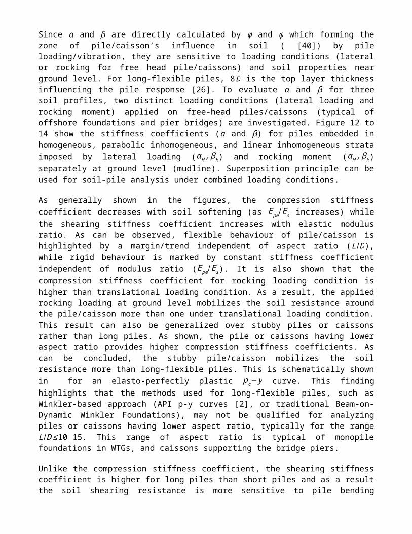
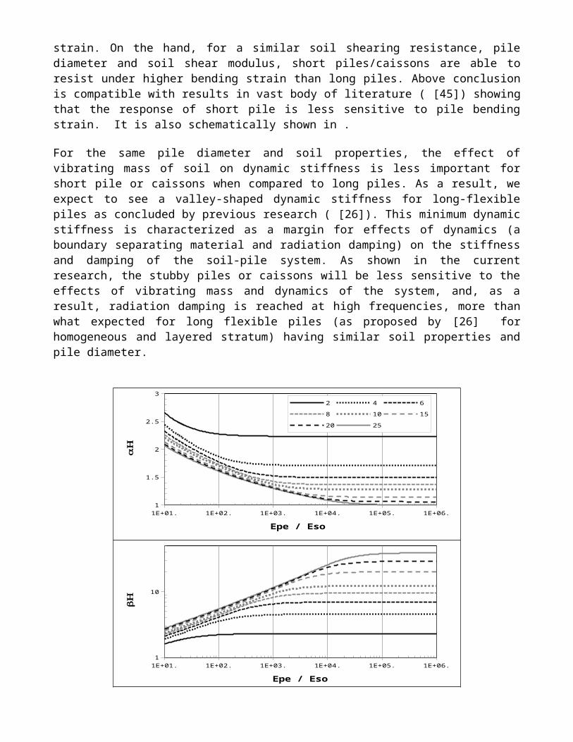
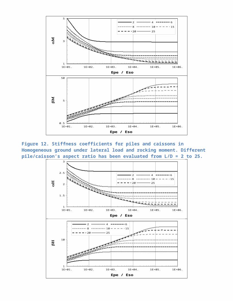
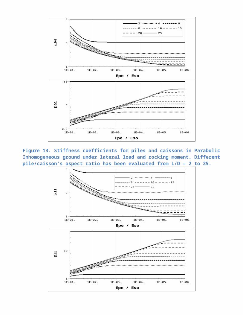
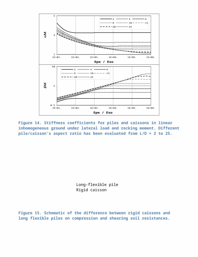
Since α and β are directly calculated by ϕ and φ which forming the zone of pile/caisson’s influence in soil ( [40]) by pile loading/vibration, they are sensitive to loading conditions (lateral or rocking for free head pile/caissons) and soil properties near ground level. For long-flexible piles, 8 D is the top layer thickness influencing the pile response [26]. To evaluate α and β for three soil profiles, two distinct loading conditions (lateral loading and rocking moment) applied on free-head piles/caissons (typical of offshore foundations and pier bridges) are investigated. Figure 12 to 14 show the stiffness coefficients (α and β) for piles embedded in homogeneous, parabolic inhomogeneous, and linear inhomogeneous strata imposed by lateral loading (αH , βH) and rocking moment (αM , βM) separately at ground level (mudline). Superposition principle can be used for soil-pile analysis under combined loading conditions.
As generally shown in the figures, the compression stiffness coefficient decreases with soil softening (as Epe /E s increases) while the shearing stiffness coefficient increases with elastic modulus ratio. As can be observed, flexible behaviour of pile/caisson is highlighted by a margin/trend independent of aspect ratio (L/D), while rigid behaviour is marked by constant stiffness coefficient independent of modulus ratio (Epe /E s). It is also shown that the compression stiffness coefficient for rocking loading condition is higher than translational loading condition. As a result, the applied rocking loading at ground level mobilizes the soil resistance around the pile/caisson more than one under translational loading condition. This result can also be generalized over stubby piles or caissons rather than long piles. As shown, the pile or caissons having lower aspect ratio provides higher compression stiffness coefficients. As can be concluded, the stubby pile/caisson mobilizes the soil resistance more than long-flexible piles. This is schematically shown in for an elasto-perfectly plastic pc− y curve. This finding highlights that the methods used for long-flexible piles, such as Winkler-based approach (API p-y curves [2], or traditional Beam-on-Dynamic Winkler Foundations), may not be qualified for analyzing piles or caissons having lower aspect ratio, typically for the range L/D≤10 15. This range of aspect ratio is typical of monopile foundations in WTGs, and caissons supporting the bridge piers.
Unlike the compression stiffness coefficient, the shearing stiffness coefficient is higher for long piles than short piles and as a result the soil shearing resistance is more sensitive to pile bending strain. On the hand, for a similar soil shearing resistance, pile diameter and soil shear modulus,
short piles/caissons are able to resist under higher bending strain than long piles. Above conclusion is compatible with results in vast body of literature ( [45]) showing that the response of short pile is less sensitive to pile bending strain. It is also schematically shown in .
For the same pile diameter and soil properties, the effect of vibrating mass of soil on dynamic stiffness is less important for short pile or caissons when compared to long piles. As a result, we expect to see a valley-shaped dynamic stiffness for long-flexible piles as concluded by previous research ( [26]). This minimum dynamic stiffness is characterized as a margin for effects of dynamics (a boundary separating material and radiation damping) on the stiffness and damping of the soil-pile system. As shown in the current research, the stubby piles or caissons will be less sensitive to the effects of vibrating mass and dynamics of the system, and, as a result, radiation damping is reached at high frequencies, more than what expected for long flexible piles (as proposed by [26] for homogeneous and layered stratum) having similar soil properties and pile diameter.
1E+01. 1E+02. 1E+03. 1E+04. 1E+05. 1E+06.1
1.5
2
2.5
3
2 4 6
8 10 15
20 25
Epe / Eso
aH
1E+01. 1E+02. 1E+03. 1E+04. 1E+05. 1E+06.1
10
Epe / Eso
bH
1E+01. 1E+02. 1E+03. 1E+04. 1E+05. 1E+06.1
3
5
2 4 6
8 10 15
20 25
Epe / Eso
aM
1E+01. 1E+02. 1E+03. 1E+04. 1E+05. 1E+06.0.5
5
50
Epe / Eso
bM
Figure 12. Stiffness coefficients for piles and caissons in Homogeneous ground under lateral load and rocking moment. Different pile/caisson’s aspect ratio has been evaluated from L/D = 2 to 25.
1E+01. 1E+02. 1E+03. 1E+04. 1E+05. 1E+06.1
1.5
2
2.5
3
2 4 6
8 10 1520 25
Epe / Eso
aH
1E+01. 1E+02. 1E+03. 1E+04. 1E+05. 1E+06.1
10
2 4 6
8 10 15
20 25
Epe / Eso
bH
1E+01. 1E+02. 1E+03. 1E+04. 1E+05. 1E+06.1
3
5
2 4 6
8 10 15
20 25
Epe / Eso
aM
1E+01. 1E+02. 1E+03. 1E+04. 1E+05. 1E+06.0.5
5
50
Epe / Eso
bM
Figure 13. Stiffness coefficients for piles and caissons in Parabolic Inhomogeneous ground under lateral load and rocking moment. Different pile/caisson’s aspect ratio has been evaluated from L/D = 2 to 25.
1E+01. 1E+02. 1E+03. 1E+04. 1E+05. 1E+06.1
2
3
2 4 6
8 10 15
20 25
Epe / Eso
aH
1E+01. 1E+02. 1E+03. 1E+04. 1E+05. 1E+06.1
10
Epe / Eso
bH
1E+01. 1E+02. 1E+03. 1E+04. 1E+05. 1E+06.1
3
5
2 4 6
8 10 15
20 25
Epe / Eso
aM
Long-flexible pileRigid caisson
1E+01. 1E+02. 1E+03. 1E+04. 1E+05. 1E+06.0.5
5
502 4 6
8 10 15
20 25
Epe / Eso
bM
Figure 14. Stiffness coefficients for piles and caissons in linear inhomogeneous ground under lateral load and rocking moment. Different pile/caisson’s aspect ratio has been evaluated from L/D = 2 to 25.
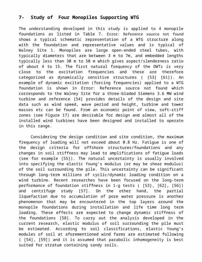
Figure 15. Schematic of the difference between rigid caissons and long flexible piles on compression and shearing soil resistances.
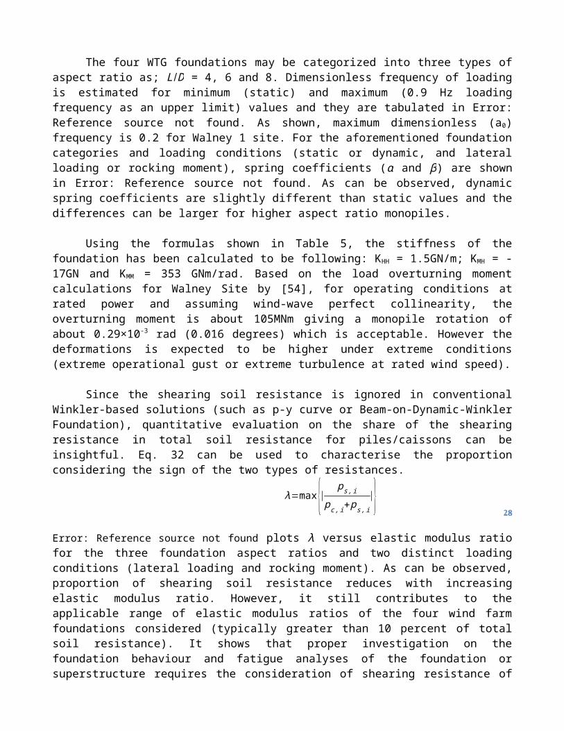
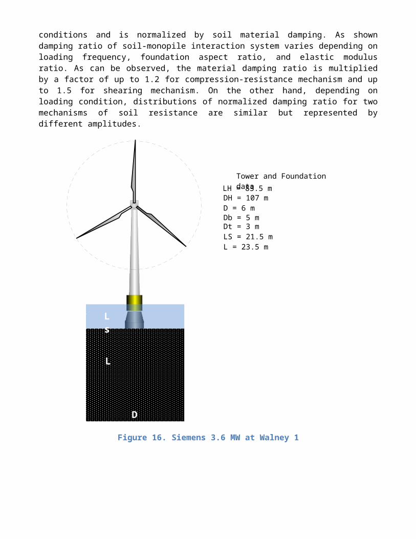
7- Study of Four Monopiles Supporting WTG
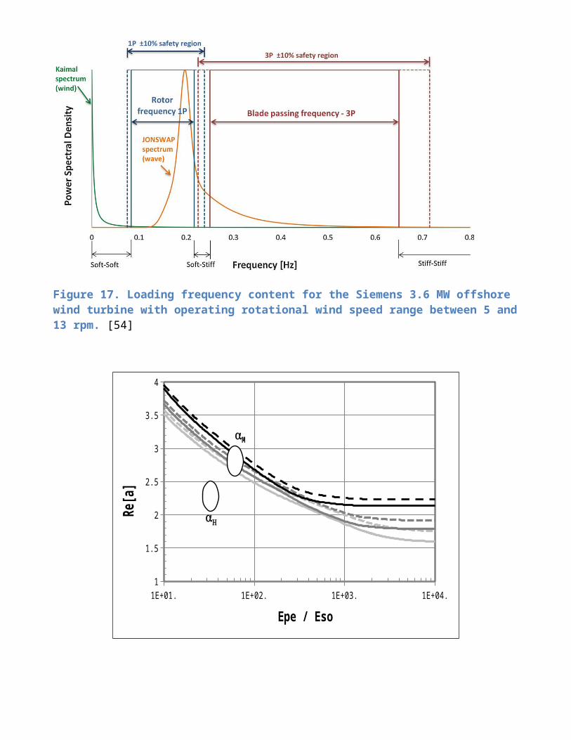
The understanding developed in this study is applied to 4 monopile foundations as listed in Table 7. Error: Reference source not found shows a typical schematic representation of a WTG structure along with the foundation and representative values and is typical of Walney Site 1. Monopiles are large open-ended steel tubes, with typically diameters that are between 3 m to 7m, and embedded lengths typically less than 30 m to 50 m which gives aspect/slenderness ratio of about 4 to 15. The first natural frequency of the OWTs is very close to the excitation frequencies and these are therefore categorized as dynamically sensitive structures ( [53] [61]). An example of dynamic excitation (forcing frequencies) applied to a WTG foundation is shown in Error:Reference source not found which corresponds to the Walney Site for a three-bladed Siemens 3.6 MW wind turbine and reference [54] provides details of the design and site data such as wind speed, wave
period and height, turbine and tower masses etc can be found. From an economic point of view, soft–stiff zones (see Figure 17) are desirable for design and almost all of the installed wind turbines have been designed and installed to operate in this range.
Considering the design condition and site condition, the maximum frequency of loading will not exceed about 0.8 Hz. Fatigue is one of the design criteria for offshore structures/foundations and any changes in soil stiffness may lead to amplifications of fatigue loads (see for example [55]). The natural uncertainty is usually involved into specifying the elastic Young’s modulus (or may be shear modulus) of the soil surrounding the pile. This uncertainty can be significant through long-term millions of cyclic/dynamic loading condition on a wind turbine. Recent researches have been focused on the long-term performance of foundation stiffness in 1-g tests ( [53], [62], [56]) and centrifuge study [57]. On the other hand, the partial liquefaction due to accumulation of pore water pressure is another phenomenon that may be encountered in the top layers around the monopile foundations during installation and life time long term loading. These effects are expected to change dynamic stiffness of the foundations [58]. To carry out the analysis developed in the current research, elastic modulus of soil surrounding the pile must be estimated. According to soil classifications, elastic Young’s modules of soil at aforementioned wind farms are estimated following ( [54], [59]) and it is assumed that parabolic inhomogeneity is best suited for stratum containing sandy soils.
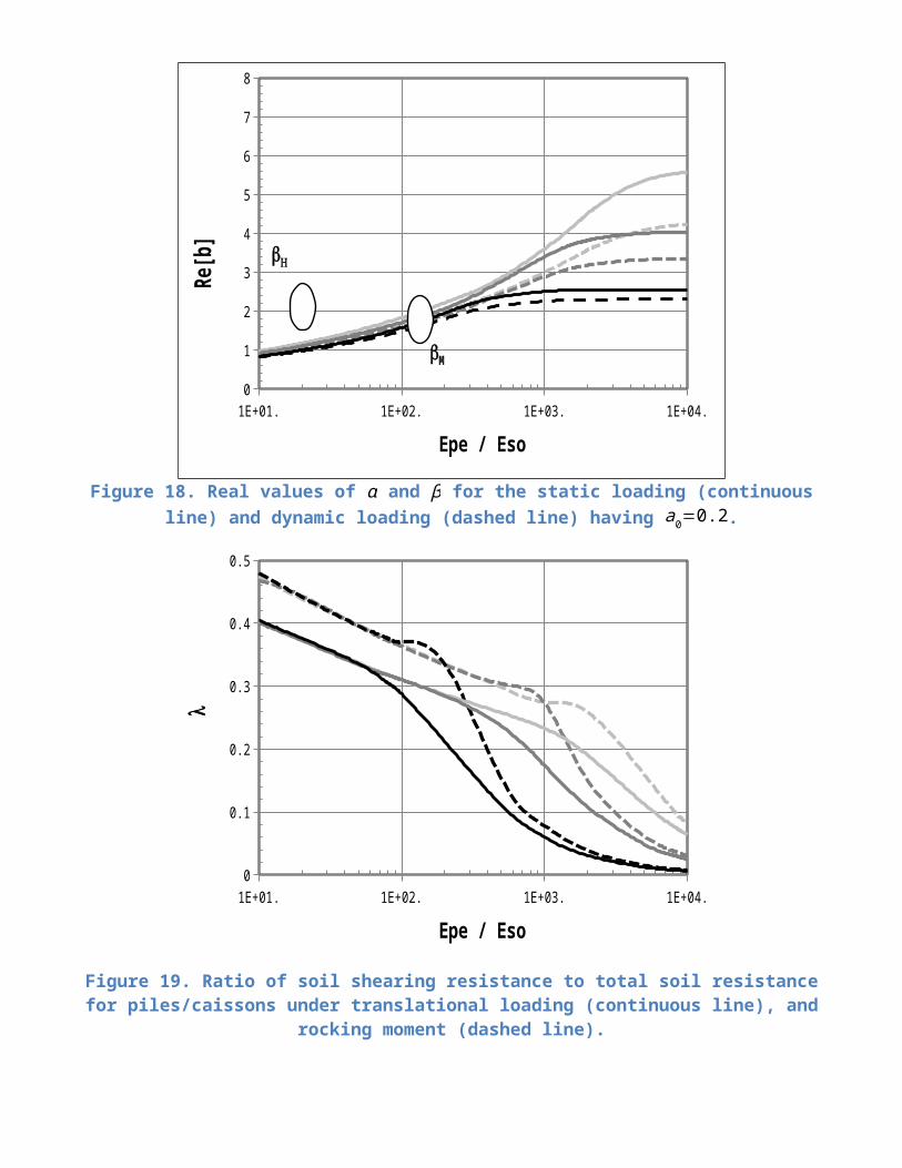
The four WTG foundations may be categorized into three types of aspect ratio as; L/D = 4, 6 and 8. Dimensionless frequency of loading is estimated for minimum (static) and maximum (0.9 Hz loading frequency as an upper limit) values and they are tabulated in Error: Reference source notfound. As shown, maximum dimensionless (a0) frequency is 0.2 for Walney 1 site. For the aforementioned foundation categories and loading conditions (static or dynamic, and lateral loading or rocking moment), spring coefficients (α and β) are shown in Error: Reference source not found. As can be observed, dynamic spring coefficients are slightly different than static values and the differences can be larger for higher aspect ratio monopiles.
Using the formulas shown in Table 5, the stiffness of the foundation has been calculated to be following: KHH = 1.5GN/m; KMH = -17GN and KMM = 353 GNm/rad. Based on the load overturning moment calculations for Walney Site by [54], for operating conditions at rated power and assuming wind-wave perfect collinearity, the overturning moment is about 105MNm giving a monopile rotation of about 0.29×10⁻³ rad (0.016 degrees) which is acceptable. However the deformations is expected to be higher under extreme conditions (extreme operational gust or extreme turbulence at rated wind speed).
Since the shearing soil resistance is ignored in conventional Winkler-based solutions (such as p-y curve or Beam-on-Dynamic-Winkler Foundation), quantitative evaluation on the share of the shearing resistance in total soil resistance for piles/caissons can be insightful. Eq. 32 can be used to characterise the proportion considering the sign of the two types of resistances.
28
λ=max {| ps , ipc , i+ ps, i
|}
Error: Reference source not found plots λ versus elastic modulus ratio for the three foundation aspect ratios and two distinct loading conditions (lateral loading and rocking moment). As can be observed, proportion of shearing soil resistance reduces with increasing elastic modulus ratio. However, it still contributes to the applicable range of elastic modulus ratios of the four wind farm foundations considered (typically greater than 10 percent of total soil resistance). It shows that proper investigation on the foundation behaviour and fatigue analyses of the foundation or superstructure requires the consideration of shearing resistance of the soil. It is derived from Error: Reference source not found that
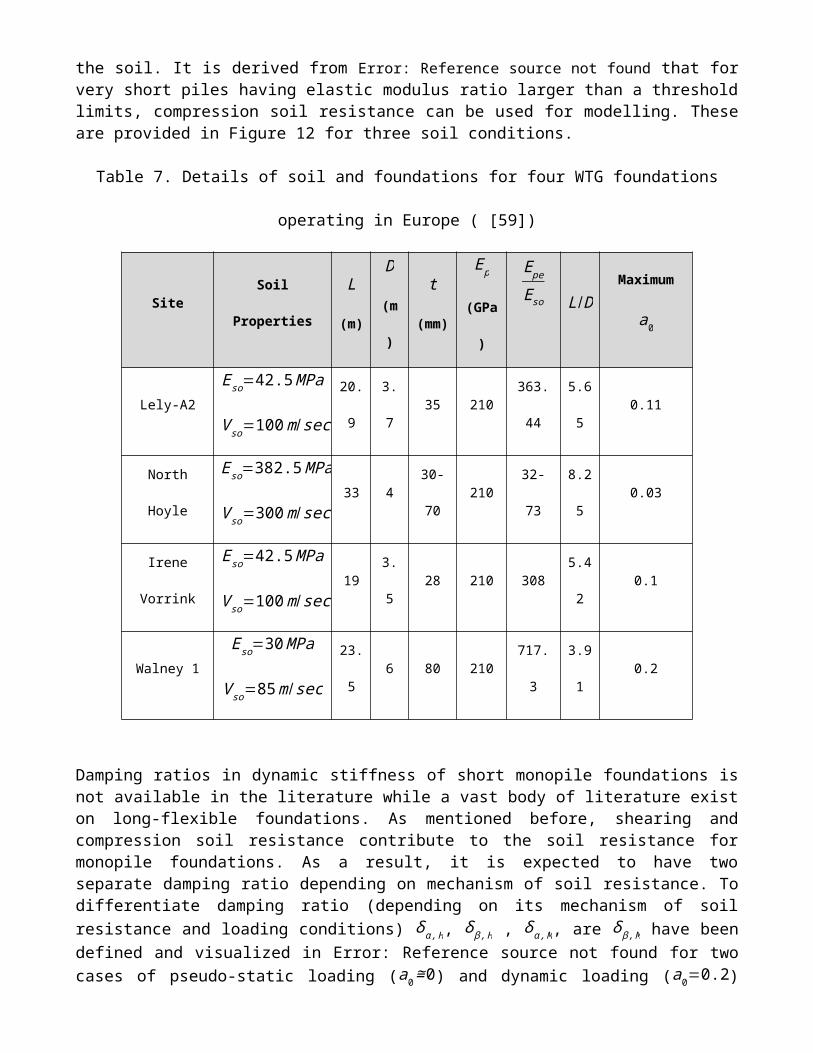
for very short piles having elastic modulus ratio larger than a threshold limits, compression soil resistance can be used for modelling. These are provided in Figure 12 for three soil conditions.
Table 7. Details of soil and foundations for four WTG foundations operating in Europe ( [59])
Site Soil PropertiesL
(m)
D
(m
)
t
(mm)
Ep
(GPa)
Epe
E so L/D Maximum a0
Lely-A2
E so=42.5 MPa
V so=100m/ sec20.9 3.7 35 210
363.4
45.65 0.11
North Hoyle
E so=382.5MPa
V so=300m/ sec33 4 30-70 210 32-73 8.25 0.03
Irene
Vorrink
E so=42.5 MPa
V so=100m/ sec19 3.5 28 210 308 5.42 0.1
Walney 1
E so=30 MPa
V so=85m /sec23.5 6 80 210 717.3 3.91 0.2
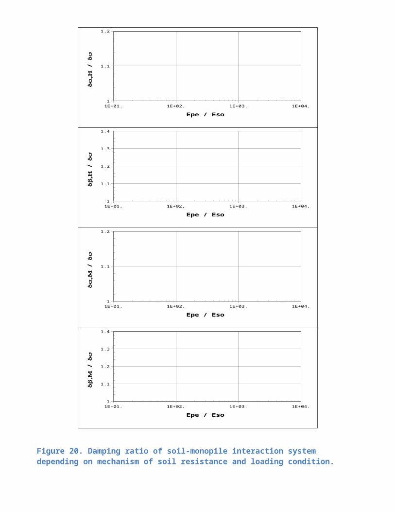
Damping ratios in dynamic stiffness of short monopile foundations is not available in the literature while a vast body of literature exist on long-flexible foundations. As mentioned before, shearing and compression soil resistance contribute to the soil resistance for monopile foundations. As a result, it is expected to have two separate damping ratio depending on mechanism of soil resistance. To differentiate damping ratio (depending on its mechanism of soil resistance and loading conditions) δ α , H, δ β , H , δ α ,M, are δ β ,M have been defined and visualized in Error: Reference source not found for two cases of pseudo-static loading (a0≅ 0) and dynamic loading (a0=0.2) conditions and is normalized by soil material damping. As shown damping ratio of soil-monopile interaction system varies depending on loading frequency, foundation aspect ratio, and elastic modulus ratio. As can be observed, the material damping ratio is multiplied by a factor of up to 1.2 for compression-resistance mechanism and up to 1.5 for shearing mechanism. On the other hand, depending on loading condition, distributions of normalized damping ratio for two mechanisms of soil resistance are similar but represented by different amplitudes.
L
Mudline
Mean Sea level
Ls
LH
DH
D
Db
Dt
Tower and Foundation data
LH = 83.5 mDH = 107 mD = 6 mDb = 5 mDt = 3 mLS = 21.5 mL = 23.5 m
Figure 16. Siemens 3.6 MW at Walney 1
Figure 17. Loading frequency content for the Siemens 3.6 MW offshore wind turbine with operating rotational wind speed range between 5 and 13 rpm. [54]
1E+01. 1E+02. 1E+03. 1E+04.1
1.5
2
2.5
3
3.5
4
Epe / Eso
Re[a
]
aM
aH
1E+01. 1E+02. 1E+03. 1E+04.0
1
2
3
4
5
6
7
8
Epe / Eso
Re[b
]
bM
bH
Figure 18. Real values of α and β for the static loading (continuous line) and dynamic loading (dashed line) having a0=0.2.
1E+01. 1E+02. 1E+03. 1E+04.0
0.1
0.2
0.3
0.4
0.5
Epe / Eso
l
Figure 19. Ratio of soil shearing resistance to total soil resistance for piles/caissons under translational loading (continuous line), and rocking moment (dashed line).
1E+01. 1E+02. 1E+03. 1E+04.1
1.1
1.2
Epe / Eso
da,H
/ ds
1E+01. 1E+02. 1E+03. 1E+04.1
1.1
1.2
1.3
1.4
Epe / Eso
db,H
/ ds
1E+01. 1E+02. 1E+03. 1E+04.1
1.1
1.2
Epe / Eso
da,M
/ ds
1E+01. 1E+02. 1E+03. 1E+04.1
1.1
1.2
1.3
1.4
Epe / Eso
db,M
/ ds
Figure 20. Damping ratio of soil-monopile interaction system depending on mechanism of soil resistance and loading condition. Pseudo-static loading (continuous line) and dynamic loading (dashed line) are marked separately.
Important observation specifically related to WTG supported on large diameter monopile foundations are:
(1) Behaviour of monopiles or caissons are more sensitive to compressional soil resistance as compared to long flexible piles because of the mobilization of the soil resistance related to the pile deformation. Also, there is considerable contributions from the shearing soil resistance depending on the elastic modulus ratio. Therefore Winkler-based approaches (such as p-y curve or Beam-on-Dynamic-Winkler Foundations) which are validated for very long-flexible piles cannot be strictly used for monopiles and caissons.
(2) If the short piles have Elastic modulus ratio (similar to pile-soil stiffness ratio) larger than a threshold limit, compressional soil resistance may be adequate to model the problem.
(3) While OWTs are dynamical sensitive structures, the current study shows that for most operational wind turbines, the estimation of dynamic stiffness of foundations is not necessary and static stiffness will be sufficient for calculations.
(4) Damping ratio is higher for monopiles as compared to long flexible piles. It is approximately 1.2δ s for mechanism arising due to compression soil resistance and 1.5δ s for mechanism of shearing soil resistance, where δ s is hysteretic damping ratio of soil. However damping ratio of monopile foundation depends on dimensionless frequency of loading, foundation aspect ratio and elastic modulus ratio. Higher damping ratio is beneficial for OWTs as it would reduce the dynamic response and also the fatigue loads.
8- Conclusion
In this study, elastodynamic solutions techniques has been used to study a wide ranges of deep foundations having different aspect ratio (representing caissons, rigid piles and flexible piles) embedded in three different ground profiles. A set of impedance functions have been proposed to obtain stiffness of the monopiles exhibiting rigid and flexible behaviour bearing in mind the current interest in WTG foundations. The solutions were compared with Finite Element analysis and other existing solutions in the literature.
Through the analysis, further understanding is developed on the applicability of uncoupled p-y curves/Winkler springs through the separation of soil resistance to laterally loaded piles into two components (shearing and compression soil resistances). The insights gained through the analysis were discussed considering four offshore wind turbine foundations from four different European wind farms. It is also shown that for deep foundations supporting Wind Turbine Generators, estimation of dynamic stiffness is not necessary and that static stiffness will be sufficient for calculations. Furthermore, damping is higher for rigid monopiles and is beneficial for the system performance of OWT (Offshore Wind Turbines) due to dynamic sensitive nature of the structure.
Acknowledgement: The work is part funded by the EPSRC (Engineering and Physical Sciences Research Council, United Kingdom) through the grant EP/H015345/2. The second author would also like to acknowledge University of Bristol for the University Senior Research Fellowship for the year 2011 to 2012.
APPENDIX
Appendix 1: Approximation of modified Bessel function of second kind.
Modified Bessel functions of second kind of order zero and order one are two solutions of soil behaviour surrounding pile in layered and inhomogeneous strata. They may be estimated by following [60]:
K 0 (x)=√ π2x
e−x [1− 18x (1− 9
16 x (1− 2524 x ))]
(1-1)
K 1 (x)=√ π2x
e− x [1+ 38 x (1− 5
16 x (1− 2124 x )) ]
(1-2)
Where x may be qr or sr.
References
[1] S. Bhattacharya, “Challenges in design of foundations for offshore wind turbines,” Engineering and Technology Reference, vol. doi:10.1049/etr.2014.0041, pp. 1-9, 2014.
[2] API, 2A (WSD): Recommended Practice for Planning, Design, and Constructing Fixed Offshore Platforms-Working Stress Design, Version 21st ed., 2000.
[3] C. LaBlanc, B. W. Byrne and G. T. Houlsby, “Response of stiff piles to random two-way lateral loading,” Geotechnique, vol. 60, no. 9, pp. 715-721, 2010.
[4] D. Kallehave, B. W. Byrne, C. LeBlanc and K. K. Mikkelsen, “Optimization of monopiles for offshore wind turbines,” Philosophical Transactions Royal Society Academy, vol. 373, p. DOI: 10.1098/rsta.2014.0100, 2015.
[5] M. Hetenyi, “Beams on Elastic Foundations,” University of Michigan, Ann Arbor, 1946.
[6] H. G. Poulos and E. H. Davis, Pile Foundation Analysis and Design, New York: John Wiley and Sons, 1980.
[7] R. L. Kuhlemeyer, “Static and dynamic laterally loaded floating piles,” Journal of Geotechnical Engineering Dicision, ASCE, vol. 105, no. GT2, pp. 289-304, 1979.
[8] M. F. Randolph, “The Response of Flexible Piles to Lateral Loading,” Geotechnique, vol. 31, no. 2, pp. 247-259, 1981.
[9] R. Dobry, E. Vicente, M. O'Rourke and J. Roesset, “Horizontal Stiffness and Damping of Single Piles,” Journal of Geotechnical Engineering Division, vol. 108, pp. 439-459, 1982.
[10] J. P. Carter and F. H. Kulhawy, “Analysis of laterally loaded shafts in rock,” ASCE Journal of Geotechnical Engineering, vol. 118, no. 6, pp. 839-855, 1992.
[11] J. P. Wolf and A. J. Deeks, Foundation vibration analysis; a strength of material approach, 1st ed., Amsterdam: Elsevier, 2004.
[12] J. P. Wolf, “Spring-dashpot-mass models for foundation vibration,” Earthquake Engineering and Structural Dynamics, vol. 26, no. 9, pp. 931-949, 1997.
[13] J. E. Luco, “Impedance functions for a rigid foundations on a layered medium,” Nuclear Engineering and Design, vol. 31, no. 2, pp. 204-217, 1974.
[14] G. Gazetas, “Formulas and Charts for Impedances of Surface and Embedded Foundations,” Journal of Geotechnical Engineering, ASCE, vol. 117, no. 9, pp. 1363-1381, 1991.
[15] D. A. Brown, J. P. Turner and R. J. Castelli, “Drilled Shafts: Construction Procedure and LRFD Design Methods,” FHWA NHI-10-016, Washington, D.C., 2010.
[16] V. Varun, D. Assimali and G. Gazetas, “A simplified model for lateral response of large diameter caisson doundations-Linear elastic foundation,” Soil Dynamics and Earthquake Engineering, vol. 29, pp. 268-291, 2009.
[17] N. Gerolymos and G. Gazetas, “Development of Winkler model for static and dynamic response of caisson foundations with soil and interface nonlinearities,” Soil Dynamics and Earthquake Engineering, vol. 26, pp. 363-376, 2006.
[18] S. Bisoi and S. Haldar, “Dynamic analysis of offshore wind turbine in clay considering soil-monopile-tower interaction,” Soil Dynamics and Earthquake Engineering, vol. 63, pp. 19-35, 2014.
[19] M. Novak, “Dynamic stiffness and damping of piles,” Canadian Geotechnical Journal, vol. 11, pp. 574-591, 1974.
[20] G. W. Blaney, E. Kausel and J. M. Roesset, “Dynamic Stiffness of Piles,” in Numerical Methods in Geomechanics, C. S. V. 2. Desai, Ed., 1976, pp. 1011-1012.
[21] A. Kaynia, “Dynamic Stiffness and Seismic Response of Pile Groups,” Research Repot R82-03, Department of Civil Engineering, MIT, Cambridge, USA, 1982.
[22] G. Gazetas, “Seismic response of end-bearing single piles,” Soil Dynamics and Earthquake Engineering, vol. 3, no. 2, pp. 82-93, 1984.
[23] F. Abedzadeh and R. Pak, “Continuum Mechanics of Lateral Soil–Pile Interaction,” Journal of Engineering Mechanics, vol. 130, no. 11, pp. 1309-1318, 2004.
[24] F. Dezzi, S. Carbonari and G. Leoni, “Kinematic bending moments in pile foundations,” Soil Dynamics and Earthquake Engineering, vol. 30, pp. 119-132, 2010.
[25] S. Haldar and D. Basu, “Response of Euler-Bernoulli beam on spatially random elastic soil,” Computers and Geotechnics, vol. 50, pp. 110-128, 2013.
[26] M. Shadlou and S. Bhattacharya, “Dynamic Stiffness of Pile in a Layered Elastic Continuum,” Geotechnique, vol. 64, no. 4, pp. 303-319, 2014.
[27] E. S. Barber, “Discussion to paper by S.M.Gleser,” ASTM,STP, vol. 154, pp. 96-99, 1953.
[28] L. C. Reese and H. Matlock, “Non-Dimensional Solutions for Laterally Loaded Piles with Soil Modulus Assumed Proportional to Depth,” in Proceeding of 8th Texas Conference on Soil Mechanics and Foundation Engineering, Special Publication, No. 29, Austin, University of Texas, Austin, 1956.
[29] H. Poulos, “The displacement of Laterally loaded piles: I- Single piles,” Journal of Soil Mechanics and Foundation Division, vol. 97, pp. 711-731, 1971 a.
[30] P. K. Banerjee and T. G. Davies, “The Behaviour of Axially and Laterally Loaded Single Piles Embedded in Non-Homogeneous Soils,” Geotechnique, vol. 28, no. 3, pp. 309-326, 1978.
[31] R. Krishnan, G. Gazetas and A. Velez, “Static and dynamic lateral deflexion of piles in non-homogeneous soil stratum,” Geotechnique, vol. 33, no. 3, pp. 307-325, 1983.
[32] G. Gazetas and R. Dobry, “Horizontal Response of Piles in Layered Soils,” Journal of Geotechnical Engineering, ASCE, vol. 110, no. 1, pp. 20-40, 1984-a.
[33] G. Gazetas and R. Dobry, “Simplified Radiation Damping Model for Piles and Foutings,” Journal of Engineering Mechanics, vol. 110, no. 6, pp. 937-956, 1984-b.
[34] R. Dobry and G. Gazetas, “Simple method for dynamic stiffness and damping of floating pile groups,” Geotechnique, vol. 38, no. 4, pp. 557-574, 1988.
[35] G. Gazetas, “Foundation Vibration,” in Foundation Engineering Handbook, H. Y. Fang, Ed., New York, Van Nostrand Reinholds, 1991, pp. 553-593.
[36] A. S. Veletsos and B. Verbic, “Lateral and rocking vibrations of footings,” ASCE Journal of Soil Mechanics and Foundations Division, vol. 97, no. SM9, p. 1227, 1971.
[37] E. Kausel, “Forced vibrations of circular foundations on layered media,” Research Report R74-11, MIT, Massachusetts, US, 1974.
[38] E. Kausel and R. Ushijima, “Vertical and torsional stiffness of cylindrical footing,” Research Report, R79-6, MIT, Massachusetts, 1979.
[39] J. L. Tasoulas and E. Kausel, “On the dynamic stiffness of circular ring footings on an elastic stratum,” International Journal of Analytical Methods in Geomechanics, vol. 8, no. 5, pp. 411-426, 1984.
[40] M. Shadlou, “Contribution to Static and Dynamic Response of Piles in Liquefiable Ground,” PhD thesis, University of Bristol, Bristol, UK, 2015.
[41] D. Basu and R. Kameswara, “Analytical solutions for Euler-Bernoulli beam on visco-elastic foundation subjected to moving load,” International Journal of Numerical and Analytical Methods in Geomechanics, vol. 37, no. 8, pp. 945-960, 2013.
[42] M. Novak and B. El Sharnouby, “Stiffness Constants of Single Piles,” Journal of Geotechnical Engineering, ASCE, vol. 109, no. 7, pp. 961-974, 1983.
[43] M. Kavvadas and G. Gazetas, “Kinematic seismic response and bending of free-head piles in layered soil,” Geotechnique, vol. 43, no. 2, pp. 207-222, 1993.
[44] M. Novak, T. Nogami and F. Aboul-Ella, “Dynamic soil reactions for plane strain case,” Journal of Engineering Mechanic Division, ASCE, vol. 104, no. 4, pp. 953-959, 1978.
[45] K. Fleming, A. Weltman, M. Randolph and K. Elson, Piling Engineering, New York: Taylor & Francis, 2009.
[46] Y. O. Barton, Laterally Loaded Model Piles in Sand: Centrifuge Tests and Finite Element Analyses, Cambridge: University of Cambridge, 1982.
[47] A. Marsland and M. F. Randolph, “Comparisond of the results from pressuremeter tests and larger in-situ tests in London Clay,” Geotechnique, vol. 27, no. 2, pp. 217-243, 1977.
[48] W. K. Elson, “Design of Laterally-Loaded Piles,” Construction Industry Research and Information Association (CIRIA), p. Report 103, 1984.
[49] S. Mazzoni, F. McKenna and G. Fenves, “Open system for earthquake engineering simulation user manual,” University of California, Berkeley, 2006. [Online]. Available: (http://opensees.berkeley.edu/OpenSees/manuals/usermanual/).
[50] M. J. Pender, “Aseismic Pile Foundation Design Analysis,” Bulletin of the New Zealand National Society for Earthquake Engineering, vol. 26, no. 1, pp. 49-160, 1993.
[51] W. Higgins and D. Basu, “Fourier finite element analysis of laterally loaded piles in elastic media,” Internal Geotechnical Report 2011-1, University of Connecticut, Storrs, Connecticut, US, 2011.
[52] A. Velez, G. Gazetas and R. Krishnan, “Lateral Dynamic Response of Constrained Head Piles,” Journal of Geitechnical Engineering, vol. 109, no. 9, pp. 1063-1081, 1983.
[53] S. Bhattacharya, J. A. Cox, D. Lombardi and D. Muir Wood, “Dynamics of offshore wind turbines supported on two foundations,” Proceeding of the ICE-Geotechnical Engineering, vol. 166, no. 2, pp. 159-169, 2012.
[54] L. Arany, S. Bhattacharya, J. Macdonald and S. J. Hogan, “Simplified critical mudline bending moment spectra of offshore wind turbine support structures,” Wind Energy, vol. DOI: 10.1002/we.1812, 2014.
[55] M. Kuhn, “Soft or stiff: a fundamental question for designers of offshore wind energy converters,” Dublin, 1997.
[56] S. Bhattacharya, T. Carrington and T. Aldridge, “Observed increases in offshore pile driving resistance,” Proceedings of the ICE-Geotechnical Engineering, vol. 162, no. 1, pp. 71-80, 2009.
[57] J. A. Cox, S. Bhattacharya, C. D. O'Loughlin, C. Gaudin, M. Cassidy and B. Bienen, “Centrifuge study on the cyclic performance of caissons in sand,” International Journal of Physical modelling in Geotechnics, vol. 14, no. 4, pp. 99-115, 2014.
[58] P. Cuéllar, M. Baeßler and W. Rücker, “Relevant factors for the liquefaction susceptibility of cyclically loaded offshore monopiles in sand,” Promechanics V, ASCE, pp. 1336-1345, 2013.
[59] S. Adhikari and S. Bhattacharya, “Dynamic analysis of wind turbine towers on flexible foundations,” Shock and Vibration, vol. 19, pp. 37-56, 2012.
[60] N. W. McLachlan, Bessel Functions for Engineers, London: Oxford University Press, 1955.
[61] L. Arany, L. , S.Bhattacharya et al (2016) Closed form solution of Eigen frequency of monopile supported offshore wind turbines in deeper waters incorporating stiffness of substructure and SSI, Soil Dynamics and Earthquake Engineering, Volume 83, April 2016, Pages 18–32
[62] Nikitas, Vimalan and Bhattacharya (2016) An innovative cyclic loading device to study long term performance of offshore wind turbines; Soil Dynamics and Earthquake Engineering; Volume 82, March 2016, Pages 154–160; doi:10.1016/j.soildyn.2015.12.008