1.1 Equations and Graphs Learning Objectives A student will be able to: Find solutions of graphs of equations. Find key properties of graphs of equations including intercepts and symmetry. Find points of intersections of two equations. Interpret graphs as models. Introduction In this lesson we will review what you have learned in previous classes about mathematical equations of relationships and corresponding graphical representations and how these enable us to address a range of mathematical applications. We will review key properties of mathematical relationships that will allow us to solve a variety of problems. We will examine examples of how equations and graphs can be used to model real-life situations. Let’s begin our discussion with some examples of algebraic equations: Example 1: y = x². The equation has ordered pairs of numbers (x, y) as solutions. Recall that a particular pair of numbers is a solution if direct substitution of the x and y values into the original equation yields a true equation statement. In this example, several solutions can be seen in the following table: We can graphically represent the relationships in a rectangular coordinate system, taking the x as the horizontal axis and the y as the vertical axis. Once we plot the individual solutions, we can draw the curve through the points to get a sketch of the graph of the relationship: We call this shape a parabola and every quadratic function, has a parabola-shaped graph. Let’s recall how we analytically find the key points on the parabola. The vertex will be the lowest point, . In
Transcript
1.1 Equations and Graphs
Learning Objectives
A student will be able to:
Find solutions of graphs of equations.
Find key properties of graphs of equations including intercepts and symmetry.
Find points of intersections of two equations.
Interpret graphs as models.
Introduction
In this lesson we will review what you have learned in previous classes about mathematical equations of relationships and
corresponding graphical representations and how these enable us to address a range of mathematical applications. We will review key properties of mathematical relationships that will allow us to solve a variety of problems. We will examine
examples of how equations and graphs can be used to model real-life situations.
Let’s begin our discussion with some examples of algebraic equations:
Example 1: y = x². The equation has ordered pairs of numbers (x, y) as solutions. Recall that a particular pair of
numbers is a solution if direct substitution of the x and y values into the original equation yields a true equation statement. In this example, several solutions can be seen in the following table:
We can graphically represent the relationships in a rectangular coordinate system, taking the x as the horizontal axis and the y as the vertical axis. Once we plot the individual solutions, we can draw the curve through the points to get a sketch
of the graph of the relationship:
We call this shape a parabola and every quadratic function, has a parabola-shaped graph.
Let’s recall how we analytically find the key points on the parabola. The vertex will be the lowest point, . In
2
general, the vertex is located at the point . We then can identify points crossing the and axes. These
are called the intercepts of the equation. The intercept is found by setting in the equation, and then solving for as follows:
The intercept is located at
The intercept is found by setting in the equation, and solving for as follows:
Using the quadratic formula, we find that . The intercepts are located at and
.
Finally, recall that we defined the symmetry of a graph. We noted examples of vertical and horizontal line symmetry as well as symmetry about particular points. For the current example, we note that the graph has symmetry in the vertical
line The graph with all of its key characteristics is summarized below:
Let’s look at a couple of more examples.
Example 2:
Here are some other examples of equations with their corresponding graphs:
3
Example 3:
We recall the first equation as linear so that its graph is a straight line. Can you determine the intercepts?
Solution:
intercept at and intercept at
Example 4:
We recall from pre-calculus that the second equation is that of a circle with center and radius Can you show
analytically that the radius is 2?
Solution:
Find the four intercepts, by setting and solving for , and then setting and solving for .
Example 5:
The third equation is an example of a polynomial relationship. Can you find the intercepts analytically?
Solution:
We can find the intercepts analytically by setting and solving for So, we have
So the intercepts are located at and Note that is also the intercept. The intercepts
can be found by setting . So, we have
4
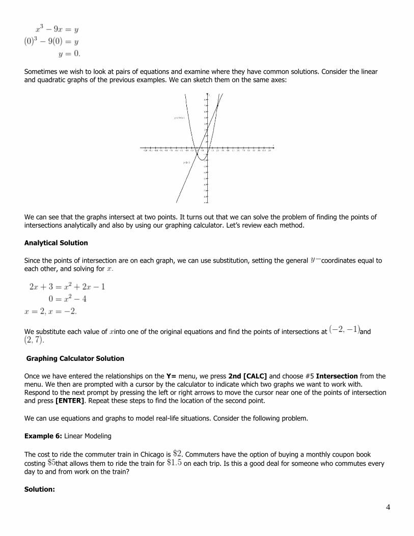
Sometimes we wish to look at pairs of equations and examine where they have common solutions. Consider the linear
and quadratic graphs of the previous examples. We can sketch them on the same axes:
We can see that the graphs intersect at two points. It turns out that we can solve the problem of finding the points of
intersections analytically and also by using our graphing calculator. Let’s review each method.
Analytical Solution
Since the points of intersection are on each graph, we can use substitution, setting the general coordinates equal to
each other, and solving for
We substitute each value of into one of the original equations and find the points of intersections at and
Graphing Calculator Solution
Once we have entered the relationships on the Y= menu, we press 2nd [CALC] and choose #5 Intersection from the
menu. We then are prompted with a cursor by the calculator to indicate which two graphs we want to work with.
Respond to the next prompt by pressing the left or right arrows to move the cursor near one of the points of intersection and press [ENTER]. Repeat these steps to find the location of the second point.
We can use equations and graphs to model real-life situations. Consider the following problem.
Example 6: Linear Modeling
The cost to ride the commuter train in Chicago is . Commuters have the option of buying a monthly coupon book
costing that allows them to ride the train for on each trip. Is this a good deal for someone who commutes every
day to and from work on the train?
Solution:
5
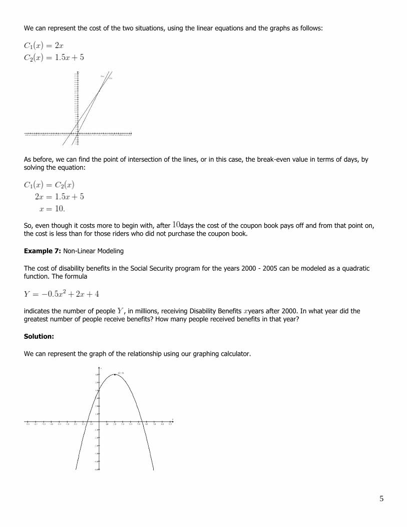
We can represent the cost of the two situations, using the linear equations and the graphs as follows:
As before, we can find the point of intersection of the lines, or in this case, the break-even value in terms of days, by
solving the equation:
So, even though it costs more to begin with, after days the cost of the coupon book pays off and from that point on,
the cost is less than for those riders who did not purchase the coupon book.
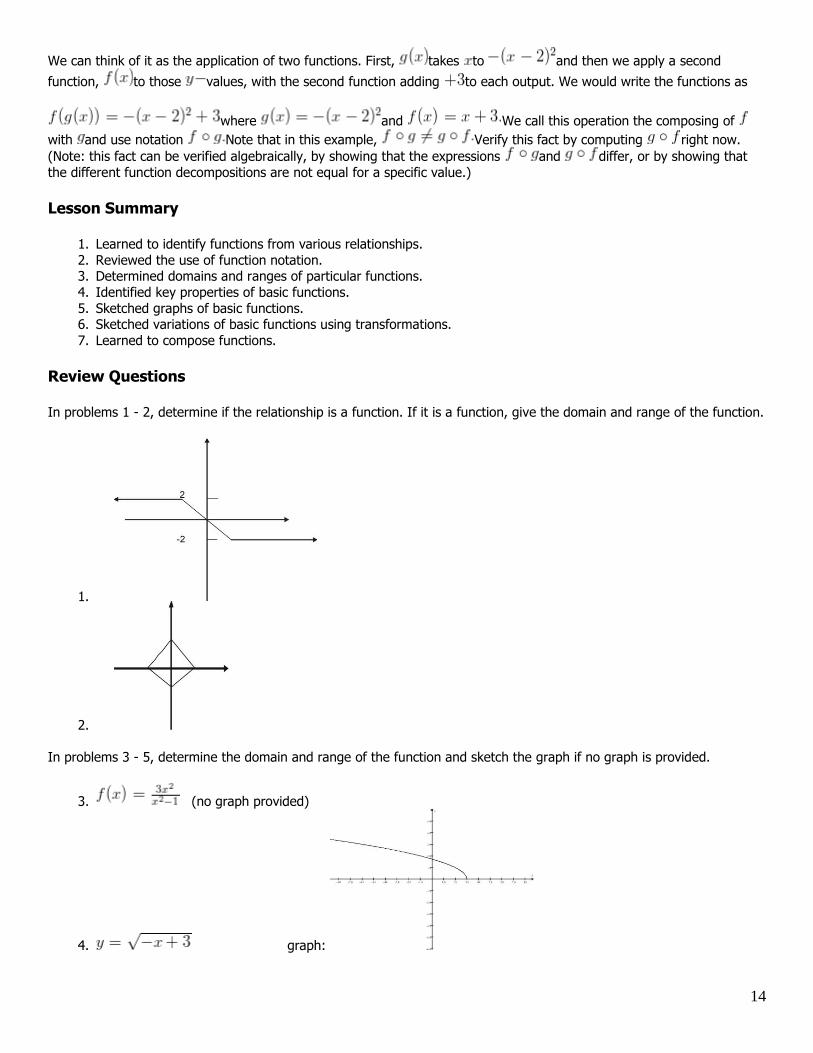
Example 7: Non-Linear Modeling
The cost of disability benefits in the Social Security program for the years 2000 - 2005 can be modeled as a quadratic function. The formula
indicates the number of people , in millions, receiving Disability Benefits years after 2000. In what year did the
greatest number of people receive benefits? How many people received benefits in that year?
Solution:
We can represent the graph of the relationship using our graphing calculator.
6
The vertex is the maximum point on the graph and is located at Hence in year 2002 a total of 6 million people
received benefits.
Lesson Summary
1. Reviewed graphs of equations
2. Reviewed how to find the intercepts of a graph of an equation and to find symmetry in the graph 3. Reviewed how relationships can be used as models of real-life phenomena
4. Reviewed how to solve problems that involve graphs and relationships
Review Questions
In each of problems 1 - 4, find a pair of solutions of the equation, the intercepts of the graph, and determine if the graph has symmetry.
1.
2.
3.
4.
7
5. Once a car is driven off of the dealership lot, it loses a significant amount of its resale value. The graph below
shows the depreciated value of a BMW versus that of a Chevy after t years. Which of the following statements is
the best conclusion about the data?
a. You should buy a BMW because they are better cars.
b. BMWs appear to retain their value better than Chevys. c. The value of each car will eventually be $0.
6. Which of the following graphs is a more realistic representation of the depreciation of cars.
7. A rectangular swimming pool has length that is 25 yards greater than its width.
a. Give the area enclosed by the pool as a function of its width.
b. Find the dimensions of the pool if it encloses an area of 264 square yards. 8. Suppose you purchased a car in 2004 for $18,000. You have just found out that the current year 2008 value of
your car is $8,500. Assuming that the rate of depreciation of the car is constant, find a formula that shows changing value of the car from 2004 to 2008.
9. For problem #8, in what year will the value of the vehicle be less than $1,400? 10. For problem #8, explain why using a constant rate of change for depreciation may not be the best way to model
depreciation.
Review Answers
1. and are two solutions. The intercepts are located at (0, -5/3) and (5/2, 0). We have a linear relationship between x and y, so its graph can be sketched as the line passing through any two solutions.
2. By solving for y, we have so two solutions are and The x-intercepts are
located at and the y-intercept is located at The graph is symmetric in the y-axis. 3. Using your graphing calculator, enter the relationship on the Y= menu. Viewing a table of points, we see many
solutions, say and and the intercepts at and By inspection we see that
the graph is symmetric about the origin.
4. Using your graphing calculator, enter the relationship on the Y= menu. Viewing a table of points, we see many
solutions, say and and the intercepts located at and By inspection we
see that the graph does not have any symmetry.
5. b. 6. c. because you would expect (1) a decline as soon as you bought the car, and (2) the value to be declining more
gradually after the initial drop. 7.
a. b. The pool has area 264 when width = 8 and length = 33.
8. The rate of change will be The formula will be
9. At the time x=7, or equivalently in the year 2011, the car will be valued at $1375. 10. A linear model may not be the best function to model depreciation because the graph of the function decreases
as time increases; hence at some point the value will take on negative real number values, an impossible
situation for the value of real goods and products.
8
1.2 Relations and Functions
Learning Objectives
A student will be able to:
Identify functions from various relationships.
Review function notation.
Determine domains and ranges of particular functions.
Identify key properties of some basic functions.
Sketch graphs of basic functions.
Sketch variations of basic functions using transformations.
Compose functions.
Introduction
In our last lesson we examined a variety of mathematical equations that expressed mathematical relationships. In this
lesson we will focus on a particular class of relationships called functions, and examine their key properties. We will then review how to sketch graphs of some basic functions that we will revisit later in this class. Finally, we will examine a way
to combine functions that will be important as we develop the key concepts of calculus.
Let’s begin our discussion by reviewing four types of equations we examined in our last lesson.
Example 1:
9
Of these, the circle has a quality that the other graphs do not share. Do you know what it is?
Solution:
The circle’s graph includes points where a particular value has two points associated with it; for example, the points
and are both solutions to the equation For each of the other relationships, a particular
value has exactly one value associated with it.)
The relationships that satisfy the condition that for each value there is a unique value are called functions. Note
that we could have determined whether the relationship satisfied this condition by a graphical test, the vertical line test. Recall the relationships of the circle, which is not a function. Let’s compare it with the parabola, which is a function.
If we draw vertical lines through the graphs as indicated, we see that the condition of a particular value having
exactly one value associated with it is equivalent to having at most one point of intersection with any vertical line. The lines on the circle intersect the graph in more than one point, while the lines drawn on the parabola intersect the graph in
exactly one point. So this vertical line test is a quick and easy way to check whether or not a graph describes a function.
We want to examine properties of functions such as function notation, their domain and range (the sets of and values
that define the function), graph sketching techniques, how we can combine functions to get new functions, and also survey some of the basic functions that we will deal with throughout the rest of this book.
Let’s start with the notation we use to describe functions. Consider the example of the linear function We
could also describe the function using the symbol and read as " of " to indicate the value of the function for a
particular value. In particular, for this function we would write and indicate the value of the function
at a particular value, say as and find its value as follows: This statement
corresponds to the solution as a point on the graph of the function. It is read, " of is ."
We can now begin to discuss the properties of functions, starting with the domain and the range of a function. The
domain refers to the set of values that are inputs in the function, while the range refers to the set of values that the function takes on. Recall our examples of functions:
Linear Function
Quadratic Function
Polynomial Function
We first note that we could insert any real number for an value and a well-defined value would come out. Hence
each function has the set of all real numbers as a domain and we indicate this in interval form as .
Likewise we see that our graphs could extend up in a positive direction and down in a negative direction without end in
either direction. Hence we see that the set of values, or the range, is the set of all real numbers
10
Example 2:
Determine the domain and range of the function.
Solution:
We note that the condition for each value is a fraction that includes an term in the denominator. In deciding what
set of values we can use, we need to exclude those values that make the denominator equal to Why? (Answer: division by is not defined for real numbers.) Hence the set of all permissible values, is all real numbers except
for the numbers which yield division by zero. So on our graph we will not see any points that correspond to
these values. It is more difficult to find the range, so let’s find it by using the graphing calculator to produce the graph.
From the graph, we see that every value in (or "All real numbers") is represented; hence the range of
the function is This is because a fraction with a non-zero numerator never equals zero.
Eight Basic Functions
We now present some basic functions that we will work with throughout the course. We will provide a list of eight basic functions with their graphs and domains and ranges. We will then show some techniques that you can use to graph
variations of these functions.
Linear
Domain All reals
Range All reals
Square (Quadratic)
Domain All reals
Range
11
Cube (Polynomial)
Domain All reals
Range All reals
Square Root
Domain
Range
Absolute Value
Domain All reals
Range
Rational
Domain
Range
Sine
Domain All reals
Range
Cosine
Domain All reals
Range
12
Graphing by Transformations
Once we have the basic functions and each graph in our memory, we can easily sketch variations of these. In general, if
we have and is some constant value, then the graph of is just the graph of shifted to the
right. Similarly, the graph of is just the graph of shifted to the left.
Example 3:
In addition, we can shift graphs up and down. In general, if we have and is some constant value, then the graph
of is just the graph of shifted up on the axis. Similarly, the graph of is just the graph
of shifted down on the axis.
Example 4:
13
We can also flip graphs in the axis by multiplying by a negative coefficient.
Finally, we can combine these transformations into a single example as follows.
Example 5:
The graph will be generated by taking flipping in the axis, and moving it two
units to the right and up three units.
Function Composition
The last topic for this lesson involves a way to combine functions called function composition. Composition of functions enables us to consider the effects of one function followed by another. Our last example of graphing by transformations
provides a nice illustration. We can think of the final graph as the effect of taking the following steps:
14
We can think of it as the application of two functions. First, takes to and then we apply a second
function, to those values, with the second function adding to each output. We would write the functions as
where and We call this operation the composing of
with and use notation Note that in this example, Verify this fact by computing right now.
(Note: this fact can be verified algebraically, by showing that the expressions and differ, or by showing that
the different function decompositions are not equal for a specific value.)
Lesson Summary
1. Learned to identify functions from various relationships.
2. Reviewed the use of function notation. 3. Determined domains and ranges of particular functions.
4. Identified key properties of basic functions.
5. Sketched graphs of basic functions. 6. Sketched variations of basic functions using transformations.
7. Learned to compose functions.
Review Questions
In problems 1 - 2, determine if the relationship is a function. If it is a function, give the domain and range of the function.
1.
2.
In problems 3 - 5, determine the domain and range of the function and sketch the graph if no graph is provided.
3. (no graph provided)
4. graph:
15
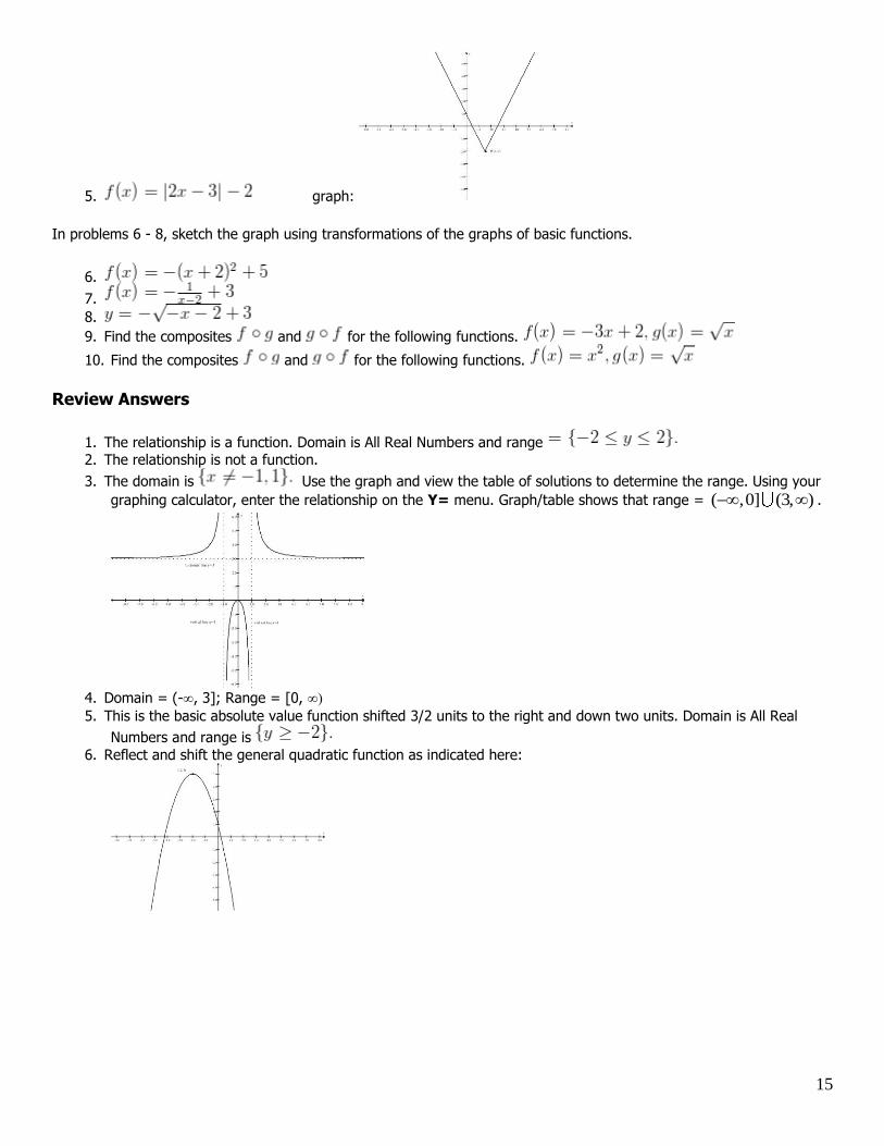
5. graph:
In problems 6 - 8, sketch the graph using transformations of the graphs of basic functions.
6.
7.
8.
9. Find the composites and for the following functions.
10. Find the composites and for the following functions.
Review Answers
1. The relationship is a function. Domain is All Real Numbers and range 2. The relationship is not a function.
3. The domain is Use the graph and view the table of solutions to determine the range. Using your
graphing calculator, enter the relationship on the Y= menu. Graph/table shows that range = ( ,0] (3, ) .
4. Domain = (-∞, 3]; Range = [0, ∞)
5. This is the basic absolute value function shifted 3/2 units to the right and down two units. Domain is All Real
Numbers and range is
6. Reflect and shift the general quadratic function as indicated here:
16
7. Reflect and shift the general rational function as indicated here:
8. Reflect and shift the general radical function as indicated here:
9. 10. ,f g x g f x ; any functions where ,f g x g f x are called inverses; in this problem f and g are
inverses of one another. Note that the domain for is restricted to only positive numbers and zero.
1.3 Models and Data
Learning Objectives
A student will be able to:
Fit data to linear models.
Fit data to quadratic models.
Fit data to trigonometric models.
Fit data to exponential growth and decay models.
Introduction
In our last lesson we examined functions and learned how to classify and sketch functions. In this lesson we will use
some classic functions to model data. The lesson will be a set of examples of each of the models. For each, we will make extensive use of the graphing calculator.
Let’s do a quick review of how to model data on the graphing calculator.
Enter Data in Lists
Press [STAT] and then [EDIT] to access the lists, L1 - L6.
17
View a Scatter Plot
Press 2nd [STAT PLOT] and choose accordingly.
Then press [WINDOW] to set the limits of the axes.
Compute the Regression Equation
Press [STAT] then choose [CALC] to access the regression equation menu. Choose the appropriate regression equation
(Linear, Quad, Cubic, Exponential, Sine).
Graph the Regression Equation Over Your Scatter Plot
Go to Y=> [MENU] and clear equations. Press [VARS], then enter and EQ and press [ENTER] (This series of entries
will copy the regression equation to your Y = screen.) Press [GRAPH] to view the regression equation over your scatter plot
Plotting and Regression in Excel
You can also do regression in an Excel spreadsheet. To start, copy and paste the table of data into Excel. With the two columns highlighted, including the column headings, click on the Chart icon and select XY scatter. Accept the defaults
until a graph appears. Select the graph, then click Chart, then Add Trendline. From the choices of trendlines choose
Linear.
Now let’s begin our survey of the various modeling situations.
Linear Models
For these kinds of situations, the data will be modeled by the classic linear equation Our task will be to find
appropriate values of and for given data.
Example 1:
It is said that the height of a person is equal to his or her wingspan (the measurement from fingertip to fingertip when your arms are stretched horizontally). If this is true, we should be able to take a table of measurements, graph the
measurements in an coordinate system, and verify this relationship. What kind of graph would you expect to see? (Answer: You would expect to see the points on the line .)
Suppose you measure the height and wingspans of nine of your classmates and gather the following data. Use your graphing calculator to see if the following measurements fit this linear model (the line ).
Height (inches) Wingspan (inches)
18
Height (inches) Wingspan (inches)
We observe that only one of the measurements has the condition that they are equal. Why aren’t more of the measurements equal to each other? (Answer: The data do not always conform to exact specifications of the model. For example, measurements tend to be loosely documented so there may be an error arising in the way that measurements were taken.)
We enter the data in our calculator in L1 and L2. We then view a scatter plot. (Caution: note that the data ranges exceed
the viewing window range of Change the window ranges accordingly to include all of the data, say )
Here is the scatter plot:
Now let us compute the regression equation. Since we expect the data to be linear, we will choose the linear
regression option from the menu. We get the equation
In general we will always wish to graph the regression equation over our data to see the goodness of fit. Doing so yields
the following graph, which was drawn with Excel:
Since our calculator will also allow for a variety of non-linear functions to be used as models, we can therefore examine
quite a few real life situations. We will first consider an example of quadratic modeling.
Quadratic Models
Example 2:
The following table lists the number of Food Stamp recipients (in millions) for each year after 1990.
19
Years after 1990 Participants
We enter the data in our calculator in L3 and L4 (that enables us to save the last example’s data). We then will view a
scatter plot. Change the window ranges accordingly to include all of the data. Use for and for
Here is the scatter plot:
Now let us compute the regression equation. Since our scatter plot suggests a quadratic model for the data, we will choose Quadratic Regression from the menu. We get the equation:
Let’s graph the equation over our data. We see the following graph:
Trigonometric Models
The following example shows how a trigonometric function can be used to model data.
Example 3:
With the skyrocketing cost of gasoline, more people have looked to mass transit as an option for getting around. The following table uses data from the American Public Transportation Association to show the number of mass transit trips
(in billions) between 1992 and 2000.
20
Year Trips (billions)
1992
1993
1994
1995
1996
1997
1998
1999
2000
We enter the data in our calculator in L5 and L6. We then will view a scatter plot. Change the window ranges accordingly
to include all of the data. Use for both and ranges.
Here is the scatter plot:
Now let us compute the regression equation. Since our scatter plot suggests a sine model for the data, we will choose
Sine Regression from the menu. We get the equation:
Let us graph the equation over our data. We see the following graph:
This example suggests that the sine over time is a function that is used in a variety of modeling situations.
Caution: Although the fit to the data appears quite good, do we really expect the number of trips to continue to go up
and down in the future? Probably not. Here is what the graph looks like when projected an additional ten years:
Exponential Models
21
Our last class of models involves exponential functions. Exponential models can be used to model growth and decay
situations. Consider the following data about the declining number of farms for the years 1980 - 2005.
Example 4:
The number of dairy farms has been declining over the past years. The following table charts the decline:
Year Farms (thousands)
1980
1985
1990
1995
2000
2005
We enter the data in our calculator in L5 (again entering the years as 1, 2, 3...) and L6. We then will view a scatter plot.
Change the window ranges accordingly to include all of the data. For the large values, choose the range
with a scale of
Here is the scatter plot:
Now let us compute the regression equation. Since our scatter plot suggests an exponential model for the data, we will
choose Exponential Regression from the menu. We get the equation:
Let’s graph the equation over our data. We see the following graph:
In the homework we will practice using our calculator extensively to model data.
Lesson Summary
1. Fit data to linear models. 2. Fit data to quadratic models.
3. Fit data to trigonometric models.
4. Fit data to exponential growth and decay models.
Review Questions
1. Consider the following table of measurements of circular objects:
22
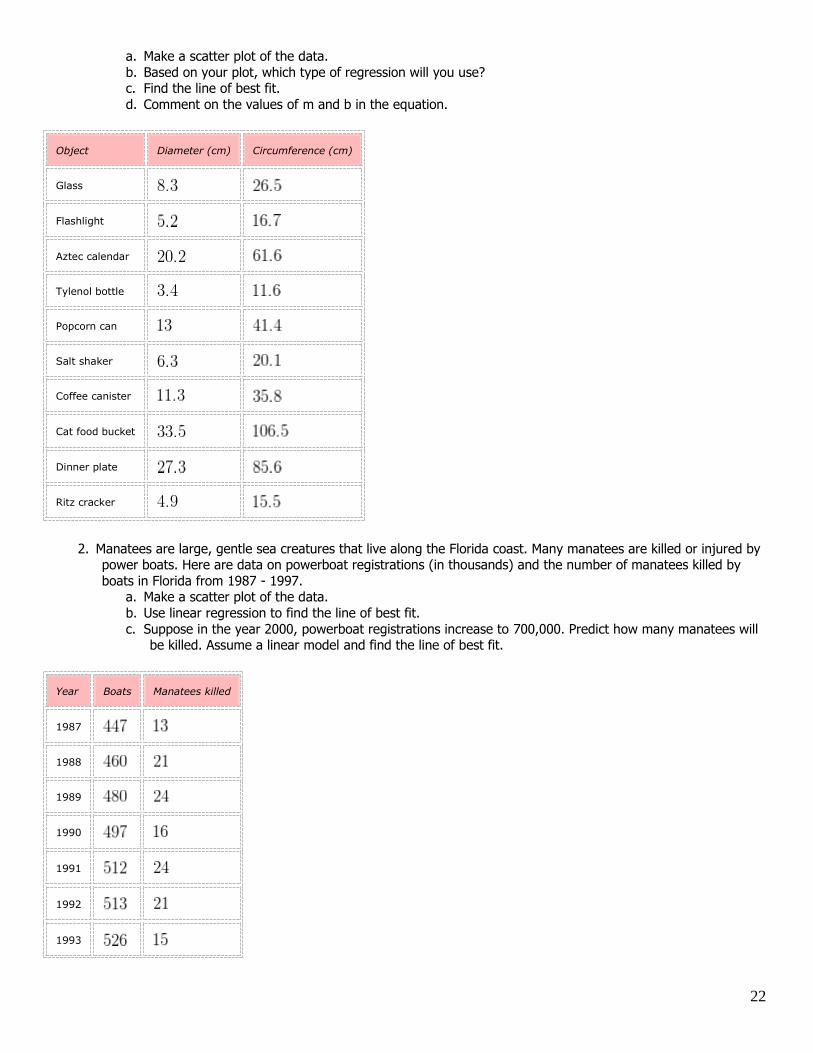
a. Make a scatter plot of the data.
b. Based on your plot, which type of regression will you use? c. Find the line of best fit.
d. Comment on the values of m and b in the equation.
Object Diameter (cm) Circumference (cm)
Glass
Flashlight
Aztec calendar
Tylenol bottle
Popcorn can
Salt shaker
Coffee canister
Cat food bucket
Dinner plate
Ritz cracker
2. Manatees are large, gentle sea creatures that live along the Florida coast. Many manatees are killed or injured by power boats. Here are data on powerboat registrations (in thousands) and the number of manatees killed by
boats in Florida from 1987 - 1997. a. Make a scatter plot of the data.
b. Use linear regression to find the line of best fit.
c. Suppose in the year 2000, powerboat registrations increase to 700,000. Predict how many manatees will be killed. Assume a linear model and find the line of best fit.
Year Boats Manatees killed
1987
1988
1989
1990
1991
1992
1993
23
Year Boats Manatees killed
1994
1995
1996
1997
3. A passage in Gulliver’s Travels states that the measurement of “Twice around the wrist is once around the neck.” The table below contains the wrist and neck measurements of 10 people.
a. Make a scatter plot of the data. b. Find the line of best fit and comment on the accuracy of the quote from the book.
c. Predict the distance around the neck of Gulliver if the distance around his wrist is found to be 52 cm.
Wrist (cm) Neck (cm)
4. The following table gives women’s average percentage of men’s salaries for the same jobs for each 5-year period
from 1960 - 2005. a. Make a scatter plot of the data.
b. Based on your sketch, should you use a linear or quadratic model for the data? c. Find a model for the data.
d. Can you explain why the data seems to dip at first and then grow?
Year Percentage
1960
1965
24
Year Percentage
1970
1975
1980
1985
1990
1995
2000
2005
5. Based on the model for the previous problem, when will women make as much as men? Is your answer a realistic prediction?
6. The average price of a gallon of gas for selected years from 1975 - 2008 is given in the following table: a. Make a scatter plot of the data.
b. Based on your sketch, should you use a linear, quadratic, or cubic model for the data? c. Find a model for the data.
d. If gas continues to rise at this rate, predict the price of gas in the year 2012.
Year Cost
1975
1976
1981
1985
1995
2005
2008
7. For the previous problem, use a linear model to analyze the situation. Does the linear method provide a better estimate for the predicted cost for the year 2011? Why or why not?
8. Suppose that you place $1,000 in a bank account where it grows exponentially at a rate of 12% continuously over the course of five years. The table below shows the amount of money you have at the end of each year.
a. Find the exponential model.
b. In what year will you triple your original amount?
Year Amount
25
Year Amount
9. Suppose that in the previous problem, you started with $3,000 but maintained the same interest rate. a. Give a formula for the exponential model. (Hint: note the coefficient and exponent in the previous
answer!) b. How long will it take for the initial amount, $3,000, to triple? Explain your answer.
10. The following table gives the average daily temperature for Indianapolis, Indiana for each month of the year.
a. Construct a scatter plot of the data. b. Find the sine model for the data.
Month Avg Temp (F)
Jan
Feb
March
April
May
June
July
Aug
Sept
Oct
Nov
Dec
Review Answers
26
1.
a. . b. Linear.
c. d. m is an estimate of , and b should be zero but due to error in measurement it is not.
2.
a. .
b. c. About 46 manatees will be killed in the year 2000. Note: there were actually 81 manatees killed in the
year 2000. 3.
a. .
b. c. 104.42 cm
4.
a. . b. Quadratic
c. d. It might be because the first wave of women into the workforce tended to take whatever jobs they could
find without regard for salary. 5. The data suggest that women will reach 100% in 2009; this is unrealistic based on current reports that women
still lag far behind men in equal salaries for equal work. 6.
a. . b. Cubic.
c. d. $12.15
7. Linear ; Predicted cost in 2012 is $4.73; it is hard to say which model works best but it seems that the use of a cubic model may overestimate the cost in the short term.
8.
a. b. the amount will triple early in Year 9.
9.
a. b. The amount will triple early in Year 9 as in the last problem because the exponential equations
and both reduce to the same equation
and hence have the same solution.
10.
27
1.4 The Calculus
Learning Objectives
A student will be able to:
Use linear approximations to study the limit process.
Compute approximations for the slope of tangent lines to a graph.
Introduce applications of differential calculus.
Introduction
In this lesson we will begin our discussion of the key concepts of calculus. They involve a couple of basic situations that
we will come back to time and again throughout the book. For each of these, we will make use of some basic ideas about how we can use straight lines to help approximate functions.
Let’s start with an example of a simple function to illustrate each of the situations.
Consider the quadratic function We recall that its graph is a parabola. Let’s look at the point on the
graph.
Suppose we magnify our picture and zoom in on the point The picture might look like this:
We note that the curve now looks very much like a straight line. If we were to overlay this view with a straight line that
intersects the curve at our picture would look like this:
We can make the following observations. First, this line would appear to provide a good estimate of the value of for
values very close to Second, the approximations appear to be getting closer and closer to the actual value of
28
the function as we take points on the line closer and closer to the point This line is called the tangent line to
at This is one of the basic situations that we will explore in calculus.
Tangent Line to a Graph
Continuing our discussion of the tangent line to at we next wish to find the equation of the tangent line. We
know that it passes though but we do not yet have enough information to generate its equation. What other
information do we need? (Answer: The slope of the line.)
Yes, we need to find the slope of the line. We would be able to find the slope if we knew a second point on the line. So
let’s choose a point on the line, very close to We can approximate the coordinates of using the function
; hence Recall that for points very close to the points on the line are close approximate
points of the function. Using this approximation, we can compute the slope of the tangent as follows:
(Note: We choose points very close to but not the point itself, so ).
In particular, for we have and Hence the equation of the tangent line,
in point slope form is We can keep getting closer to the actual value of the slope by taking
closer to or closer and closer to as in the following table:
As we get closer to we get closer to the actual slope of the tangent line, the value We call the slope of the
tangent line at the point the derivative of the function at the point
Let’s make a couple of observations about this process. First, we can interpret the process graphically as finding secant
lines from to other points on the graph. From the diagram we see a sequence of these secant lines and can observe
how they begin to approximate the tangent line to the graph at The diagram shows a pair of secant lines, joining
with points and
29
Second, in examining the sequence of slopes of these secants, we are systematically observing approximate slopes of
the function as point gets closer to Finally, producing the table of slope values above was an inductive process in which we generated some data and then looked to deduce from our data the value to which the generated results
tended. In this example, the slope values appear to approach the value This process of finding how function values behave as we systematically get closer and closer to particular values is the process of finding limits. In the next
lesson we will formally define this process and develop some efficient ways for computing limits of functions.
Applications of Differential Calculus
Maximizing and Minimizing Functions
Recall from Lesson 1.3 our example of modeling the number of Food Stamp recipients. The model was found to be
with graph as follows: (Use viewing window ranges of on and on )
We note that the function appears to attain a maximum value about an value somewhere around Using the
process from the previous example, what can we say about the tangent line to the graph for that value that yields the
maximum value (the point at the top of the parabola)? (Answer: the tangent line will be horizontal, thus having a slope of .)
Hence we can use calculus to model situations where we wish to maximize or minimize a particular function. This process
will be particularly important for looking at situations from business and industry where polynomial functions provide
accurate models.
Velocity of a Falling Object
We can use differential calculus to investigate the velocity of a falling object. Galileo found that the distance traveled by a
falling object was proportional to the square of the time it has been falling:
The average velocity of a falling object from to is given by
HW Problem #10 will give you an opportunity to explore this relationship. In our discussion, we saw how the study of tangent lines to functions yields rich information about functions. We now consider the second situation that arises in
Calculus, the central problem of finding the area under the curve of a function .
Area Under a Curve
30
First let’s describe what we mean when we refer to the area under a curve. Let’s reconsider our basic quadratic function
Suppose we are interested in finding the area under the curve from to
We see the cross-hatched region that lies between the graph and the axis. That is the area we wish to compute. As
with approximating the slope of the tangent line to a function, we will use familiar linear methods to approximate the area. Then we will repeat the iterative process of finding better and better approximations.
Can you think of any ways that you would be able to approximate the area? (Answer: One ideas is that we could compute
the area of the square that has a corner at to be and then take half to find an area This is one
estimate of the area and it is actually a pretty good first approximation.)
We will use a variation of this covering of the region with quadrilaterals to get better approximations. We will do so by dividing the interval from to into equal sub-intervals. Let’s start by using four such subintervals as
indicated:
We now will construct four rectangles that will serve as the basis for our approximation of the area. The subintervals will serve as the width of the rectangles. We will take the length of each rectangle to be the maximum value of the function
in the subinterval. Hence we get the following figure:
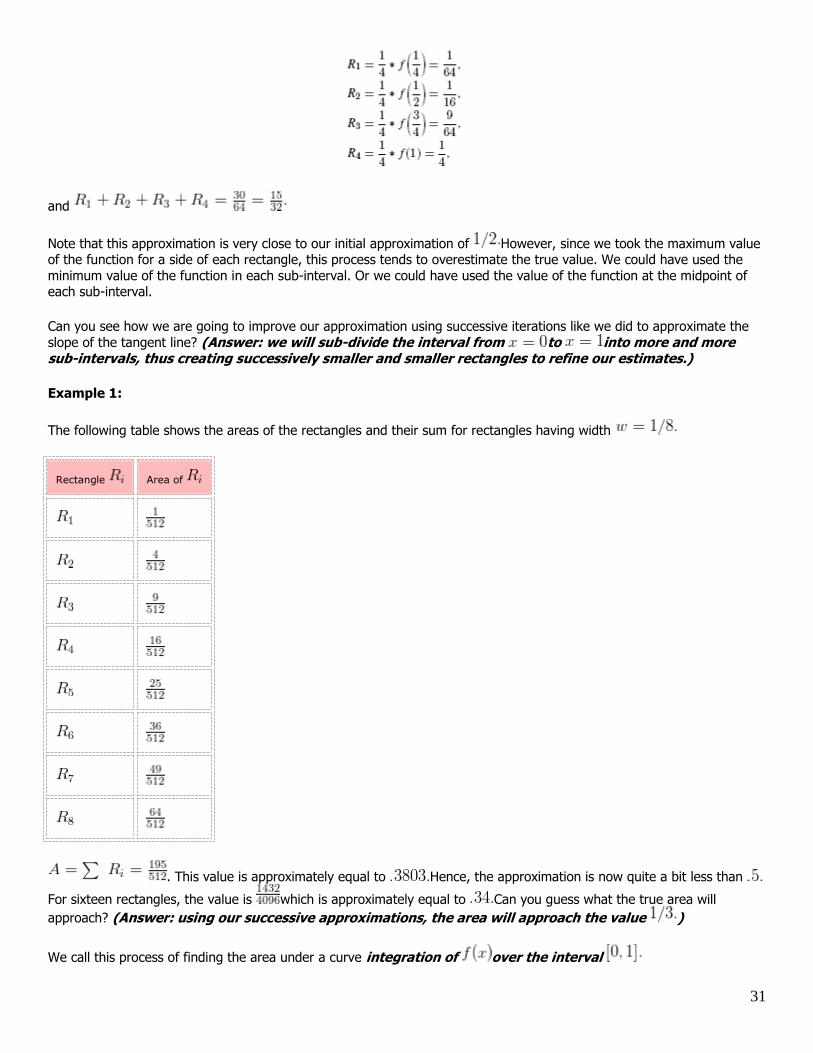
If we call the rectangles R1–R4, from left to right, then we have the areas
31
and
Note that this approximation is very close to our initial approximation of However, since we took the maximum value of the function for a side of each rectangle, this process tends to overestimate the true value. We could have used the
minimum value of the function in each sub-interval. Or we could have used the value of the function at the midpoint of each sub-interval.
Can you see how we are going to improve our approximation using successive iterations like we did to approximate the
slope of the tangent line? (Answer: we will sub-divide the interval from to into more and more sub-intervals, thus creating successively smaller and smaller rectangles to refine our estimates.)
Example 1:
The following table shows the areas of the rectangles and their sum for rectangles having width
Rectangle Area of
. This value is approximately equal to Hence, the approximation is now quite a bit less than
For sixteen rectangles, the value is which is approximately equal to Can you guess what the true area will
approach? (Answer: using our successive approximations, the area will approach the value )
We call this process of finding the area under a curve integration of over the interval
32
Applications of Integral Calculus
We have not yet developed any computational machinery for computing derivatives and integrals so we will just state
one popular application of integral calculus that relates the derivative and integrals of a function.
Example 2:
There are quite a few applications of calculus in business. One of these is the cost function of producing items of a
product. It can be shown that the derivative of the cost function that gives the slope of the tangent line is another
function that that gives the cost to produce an additional unit of the product. This is called the marginal cost and is a very important piece of information for management to have. Conversely, if one knows the marginal cost as a function of
then finding the area under the curve of the function will give back the cost function
Lesson Summary
1. We used linear approximations to study the limit process. 2. We computed approximations for the slope of tangent lines to a graph.
3. We analyzed applications of differential calculus. 4. We analyzed applications of integral calculus.
Review Questions
1. For the function approximate the slope of the tangent line to the graph at the point Use the
following set of x-values to generate the sequence of secant line slopes: What value does the sequence of slopes approach?
2. Consider the function
a. For what values of x would you expect the slope of the tangent line to be negative?
b. For what value of x would you expect the tangent line to have slope m = 0? c. Give an example of a function that has two different horizontal tangent lines.
3. Consider the function Generate the graph of using your calculator.
a. Approximate the slope of the tangent line to the graph at the point Use the following set of
x-values to generate the sequence of secant line slopes. b. For what values of x do the tangent lines appear to have slope of 0? (Hint: Use the calculate function in
your calculator to approximate the x-values.)
c. For what values of x do the tangent lines appear to have positive slope? d. For what values of x do the tangent lines appear to have negative slope?
4. The cost of producing x Hi-Fi stereo receivers by Yamaha each week is modeled by the following function:
a. Generate the graph of C(x) using your calculator. (Hint: Change your viewing window to reflect the high y values.)
b. For what number of units will the function be maximized?
c. Estimate the slope of the tangent line at
d. Where is marginal cost positive?
5. Find the area under the curve of from x = 1 to x = 3. Use a rectangle method that uses the
minimum value of the function within sub-intervals. Produce the approximation for each case of the subinterval cases.
a. four sub-intervals. b. eight sub-intervals.
c. Repeat part a. using a Mid-Point Value of the function within each sub-interval. d. Which of the answers in a. - c. provide the best estimate of the actual area?
6. Consider the function
33
a. Find the area under the curve from x = 0 to x = 1.
b. Can you find the area under the curve from x = -1 to x = 0? Why or why not? What is problematic for this computation?
7. Find the area under the curve of from x = 1 to x = 4. Use the Max Value rectangle method with six sub-intervals to compute the area.
8. The Eiffel Tower is 320 meters high. Suppose that you drop a ball off the top of the tower. The distance that it
falls is a function of time and is given by Find the velocity of the ball after 4 seconds. (Hint: the average velocity for a time interval is average velocity = change in distance/change in time. Investigate
the average velocity for t intervals close to t = 4 such as 3.9 t 4 and closer and see if a pattern is evident.)
Review Answers
1. m = 6
2. a. For
b. At the tangent line is horizontal and thus has slope of 0.
c. Many different examples; for instance, a polynomial function such as
3.
a. Slope tends toward
b. .57x
c. ( , .57) (.57, )
d. ( .57,.57)
4.
a. 80, 20, -40 b. 333 units
c. 80, 20, -40
d. x < 333 5.
a. 6.75 b. 7.6875
c. 8.625 d. Part c.
6.
a. 1.75 b. The graph drops below the x-axis into the third quadrant. Hence we are not finding the area below the
curve but actually the area between the curve and the x-axis. But note that the curve is symmetric about the origin. Hence the region from x = -1 to x = 0 will have the same area as the region from
x = 0 to x = 1.
7. 4.911 8. 39.2 m/s
1.5 Finding Limits
Learning Objectives
A student will be able to:
Find the limit of a function numerically.
Find the limit of a function using a graph.
Identify cases when limits do not exist.
Use the formal definition of a limit to solve limit problems.
Introduction
34
In this lesson we will continue our discussion of the limiting process we introduced in Lesson 1.4. We will examine
numerical and graphical techniques to find limits where they exist and also to examine examples where limits do not exist. We will conclude the lesson with a more precise definition of limits.
Let’s start with the notation that we will use to denote limits. We indicate the limit of a function as the values approach
a particular value of say as
So, in the example from Lesson 1.3 concerning the function we took points that got closer to the point on the
graph and observed the sequence of slope values of the corresponding secant lines. Using our limit notation here, we would write
Recall also that we found that the slope values tended to the value ; hence using our notation we can write
Finding Limits Numerically
In our example in Lesson 1.3 we used this approach to find that . Let’s apply this technique to a more
complicated function.
Consider the rational function . Let’s find the following limit:
Unlike our simple quadratic function, it is tedious to compute the points manually. So let’s use the [TABLE]
function of our calculator. Enter the equation in your calculator and examine the table of points of the function. Do you
notice anything unusual about the points? (Answer: There are error readings indicated for because the function is not defined at these values.)
Even though the function is not defined at we can still use the calculator to read the values for values very
close to Press 2ND [TBLSET] and set Tblstart to and to (see screen on left below). The resulting
table appears in the middle below.
Can you guess the value of ? If you guessed you would be correct. Before we finalize our answer, let’s get even closer to and determine its function value using the [CALC VALUE] tool.
35
Press 2ND [TBLSET] and change Indpnt from Auto to Ask. Now when you go to the table, enter and
press [ENTER] and you will see the screen on the right above. Press [ENTER] and see that the function value is
which is the closest the calculator can display in the four decimal places allotted in the table. So our guess is
correct and .
Finding Limits Graphically
Let’s continue with the same problem but now let’s focus on using the graph of the function to determine its limit.
We enter the function in the menu and sketch the graph. Since we are interested in the value of the function for
close to we will look to [ZOOM] in on the graph at that point.
Our graph above is set to the normal viewing window Hence the values of the function appear to be very close
to . But in our numerical example, we found that the function values approached To see this graphically, we can use the [ZOOM] and [TRACE] function of our calculator. Begin by choosing [ZOOM] function and
choose [BOX]. Using the directional arrows to move the cursor, make a box around the value (See the screen on the left below Press [ENTER] and [TRACE] and you will see the screen in the middle below.) In [TRACE] mode, type
the number and press [ENTER]. You will see a screen like the one on the right below.
The graphing calculator will allow us to calculate limits graphically, provided that we have the function rule for the function so that we can enter its equation into the calculator. What if we have only a graph given to us and we are asked
to find certain limits?
It turns out that we will need to have pretty accurate graphs that include sufficient detail about the location of data
points. Consider the following example.
Example 1:
Find for the function pictured here. Assume units of value 1 for each unit on the axes.
36
By inspection, we see that as we approach the value from the left, we do so along what appears to be a portion of
the horizontal line We see that as we approach the value from the right, we do so along a line segment
having positive slope. In either case, the values of approaches
Nonexistent Limits
We sometimes have functions where does not exist. We have already seen an example of a function where
our a value was not in the domain of the function. In particular, the function was not defined for but we
could still find the limit as
What do you think the limit will be as we let
Our inspection of the graph suggests that the function around does not appear to approach a particular value. For
the points all lie in the first quadrant and appear to grow very quickly to large positive numbers as we get close to
Alternatively, for we see that the points all lie in the fourth quadrant and decrease to large negative
numbers. If we inspect actual values very close to we can see that the values of the function do not approach a
particular value.
For this example, we say that does not exist.
Formal Definition of a Limit
37
We conclude this lesson with a formal definition of a limit.
Definition:
This definition is somewhat intuitive to us given the examples we have covered. Geometrically, the definition
means that for any lines below and above the line , there exist vertical lines
to the left and right of so that the graph of between and lies
between the lines and . The key phrase in the above statement is “for every open interval ”,
which means that even if is very, very small (that is, is very, very close to ), it still is possible to find
interval where is defined for all values except possibly .
We say that the limit of a function at is written as , if for every open interval of
there exists an open interval of that does not include such that is in for every in
Example 2:
Use the definition of a limit to prove that
We need to show that for each open interval of , we can find an open neighborhood of , that does not include , so that all in the open neighborhood map into the open interval of .
Equivalently, we must show that for every interval of say we can find an interval of , say
such that whenever
The first inequality is equivalent to and solving for we have
Hence if we take , we will have
Fortunately, we do not have to do this to evaluate limits. In Lesson 1.6 we will learn several rules that will make the task manageable.
Lesson Summary
1. We learned to find the limit of a function numerically.
2. We learned to find the limit of a function using a graph. 3. We identified cases when limits do not exist.
4. We used the formal definition of a limit to solve limit problems.
38
Multimedia Links
For another look at the definition of a limit, the series of videos at Tutorials for the Calculus Phobe has a nice intuitive
introduction to this fundamental concept (despite the whimsical name). If you want to experiment with limits yourself,
follow the sequence of activities using a graphing applet at Informal Limits. Directions for using the graphing applets at this very useful site are also available at Applet Intro.
Review Questions
1. Use a table of values to find . Use x-values of x = -1.9, -1.99, -1.999, -2.1, -2.01, -2.001. What
value does the sequence of values approach?
2. Use a table of values to find . Use values of x = .49, .499, .4999, .51, .501, .5001. What
value does the sequence of values approach?
3. Consider the function Generate the graph of p(x) using your calculator. Find each of the following limits if they exist. Use tables with appropriate values to determine the limits.
a.
b.
c. d. Find the values of the function corresponding to x = 4, -4, 0. How do these function values compare to
the limits you found in #a-c? Explain your answer.
4. Examine the graph of f(x) below to approximate each of the following limits if they exist.
a.
b.
c.
d. 5. Examine the graph of f(x) below to approximate each of the following limits if they exist.
a.
b.
c.
d.
In problems #6-8, determine if the indicated limit exists, and if so, find the limit. Provide a numerical argument to justify your answer.
In problems #9-10, determine if the indicated limit exists. Provide a graphical argument to justify your answer. (Hint: Make use of the [ZOOM] and [TABLE] functions of your calculator to view functions values close to the indicated x
value.
9.
10.
Review Answers
1. -4 2. 2/5
3. a. lim as x -> 4 of (3x³ - 3x) = 180
b. lim as x -> -4 of (3x³ - 3x) = -180
c. d. They are the same values because the function is defined for each of these x-values.
4.
a.
b.
c.
d. does not exist.
5.
a.
b. does not exist.
c. is some number close to 1 and less than 1, but not equal to 1.
d. is some number close to 1 and less than 1, but not equal to 1. 6. The limit does exist. This can be verified by using the [TRACE] or [TABLE] function of your calculator, applied
to x values very close to . The limit is 7. 7. The limit does exist. This can be verified by using the [TRACE] or [TABLE] function of your calculator, applied
to x values very close to . The limit is -1/2.
8. The limit does exist. This can be verified by using the [TRACE] or [TABLE] function of your calculator, applied to x values very close to . The limit is 1.
9. The limit does exist. This can be verified with either the [TRACE] or [TABLE] function of your calculator. 10. The limit does not exist; [ZOOM] in on the graph around x = -1 and see that the y-values approach a different
value when approached from the right and from the left.
1.6 Evaluating Limits
Learning Objectives
A student will be able to:
Find the limit of basic functions.
Use properties of limits to find limits of polynomial, rational and radical functions.
Find limits of composite functions.
Find limits of trigonometric functions.
Use the Squeeze Theorem to find limits.
Introduction
40
In this lesson we will continue our discussion of limits and focus on ways to evaluate limits. We will observe the limits of a
few basic functions and then introduce a set of laws for working with limits. We will conclude the lesson with a theorem that will allow us to use an indirect method to find the limit of a function.
Direct Substitution and Basic Limits
Let’s begin with some observations about limits of basic functions. Consider the following limit problems:
These are examples of limits of basic constant and linear functions, and
We note that each of these functions are defined for all real numbers. If we apply our techniques for finding the limits we
see that
and observe that for each the limit equals the value of the function at the value of interest:
Hence . This will also be true for some of our other basic functions, in particular all polynomial and
radical functions, provided that the function is defined at . For example, and
. The properties of functions that make these facts true will be discussed in Lesson 1.7. For now, we wish to use this idea for evaluating limits of basic functions. However, in order to evaluate limits of more
complex function we will need some properties of limits, just as we needed laws for dealing with complex problems involving exponents. A simple example illustrates the need we have for such laws.
Example 1:
Evaluate . The problem here is that while we know that the limit of each individual function of the
sum exists, and , our basic limits above do not tell us what happens when we find the limit of a sum of functions. We will state a set of properties for dealing with such sophisticated functions.
Properties of Limits
Suppose that and both exist. Then
1. where is a real number,
2. where is a real number,
3.
4.
5. provided that
41
With these properties we can evaluate a wide range of polynomial and radical functions. Recalling our example above, we
see that
Find the following limit if it exists:
Since the limit of each function within the parentheses exists, we can apply our properties and find
Observe that the second limit, , is an application of Law #2 with . So we have
In most cases of sophisticated functions, we simplify the task by applying the Properties as indicated. We want to examine a few exceptions to these rules that will require additional analysis.
Strategies for Evaluating Limits of Rational Functions
Let’s recall our example
We saw that the function did not have to be defined at a particular value for the limit to exist. In this example, the
function was not defined for . However we were able to evaluate the limit numerically by checking functional values
around and found .
Note that if we tried to evaluate by direct substitution, we would get the quantity , which we refer to as an
indeterminate form. In particular, Property #5 for finding limits does not apply since . Hence in
order to evaluate the limit without using numerical or graphical techniques we make the following observation. The
numerator of the function can be factored, with one factor common to the denominator, and the fraction simplified as follows:
In making this simplification, we are indicating that the original function can be viewed as a linear function for values close to but not equal to , that is,
for . In terms of our limits, we can say
Example 2:
Find
42
This is another case where direct substitution to evaluate the limit gives the indeterminate form . Reducing the fraction as before gives:
Example 3:
In order to evaluate the limit, we need to recall that the difference of squares of real numbers can be factored as
We then rewrite and simplify the original function as follows:
Hence .
You will solve similar examples in the homework where some clever applications of factoring to reduce fractions will enable you to evaluate the limit.
Limits of Composite Functions
While we can use the Properties to find limits of composite functions, composite functions will present some difficulties that we will fully discuss in the next Lesson. We can illustrate with the following examples, one where the limit exists and
the other where the limit does not exist.
Example 4:
Consider . Find .
We see that and note that property #5 does hold. Hence by direct substitution we have
Example 5:
Consider Then we have that is undefined and we get the indeterminate form .
Hence does not exist.
Limits of Trigonometric Functions
In evaluating limits of trigonometric functions we will look to rely more on numerical and graphical techniques due to the unique behavior of these functions. Let’s look at a couple of examples.
Example 6:
Find .
43
We can find this limit by observing the graph of the sine function and using the [CALC VALUE] function of our calculator
to show that .
While we could have found the limit by direct substitution, in general, when dealing with trigonometric functions, we will
rely less on formal properties of limits for finding limits of trigonometric functions and more on our graphing and
numerical techniques.
The following theorem provides us a way to evaluate limits of complex trigonometric expressions.
Squeeze Theorem
Suppose that for near , and .
Then .
In other words, if we can find bounds for a function that have the same limit, then the limit of the function that they
bound must have the same limit.
Example 7:
Find .
From the graph we note that:
1. The function is bounded by the graphs of and
2. .
Hence the Squeeze Theorem applies and we conclude that
Lesson Summary
1. We learned to find the limit of basic functions. 2. We learned to find the limit of polynomial, rational and radical functions.
3. We learned how to find limits of composite and trigonometric functions.
4. We used the Squeeze Theorem to find special limits.
Multimedia Links
For an introduction to finding limits (1.0), see Math Video Tutorials by James Sousa, Introduction to Limits
9. Consider function such that for Use the Squeeze Theorem to
find .
10. Use the Squeeze Theorem to show that
Review Answers
1.
2.
3.
4. does not exist.
5.
6.
7.
8. does not exist since is undefined.
9. since
10. Note that , and since , then by the Squeeze Theorem
we must have .
1.7 Continuity
Learning Objectives
A student will be able to:
Learn to examine continuity of functions.
Find one-sided limits.
Understand properties of continuous functions.
Solve problems using the Min-Max theorem.
Solve problems using the Intermediate Value Theorem.
Introduction
In this lesson we will discuss the property of continuity of functions and examine some very important implications. Let’s
start with an example of a rational function and observe its graph. Consider the following function:
We know from our study of domains that in order for the function to be defined, we must use Yet when we generate the graph of the function (using the standard viewing window), we get the following picture that appears to be
defined at :
46
The seeming contradiction is due to the fact that our original function had a common factor in the numerator and
denominator, that cancelled out and gave us a picture that appears to be the graph of
But what we actually have is the original function, that we know is not defined at
At we have a hole in the graph, or a discontinuity of the function at That is, the function is defined for
all other values close to
Loosely speaking, if we were to hand-draw the graph, we would need to take our pencil off the page when we got to this hole, leaving a gap in the graph as indicated:
Now we will formalize the property of continuity of a function and provide a test for determining when we have continuous functions.
Continuity of a Function
Definition:
The function is continuous at if the following conditions all hold:
1. is in the domain of ;
2. exists;
3.
Note that it is possible to have functions where two of these conditions are satisfied but the third is not.
Consider the piecewise function
47
In this example we have exists, is in the domain of , but .
One-Sided Limits and Closed Intervals
Let’s recall our basic square root function, .
Since the domain of is , we see that that does not exist. Specifically, we cannot find open
intervals around that satisfy the limit definition. However we do note that as we approach from the right-
hand side, we see the successive values tending towards . This example provides some rationale for how we can define one-sided limits.
Definition:
Similarly, we say that the left-hand limit of at is , written as , if for every open
interval of there exists an open interval contained in the domain of such that is in for
every in
For the example above, we write
We say that the right-hand limit of a function at is , written as , if for every open
interval of , there exists an open interval contained in the domain of such that is in
for every in
48
Example 1:
Find
The graph has a discontinuity at as indicated:
We see that and also that .
Properties of Continuous Functions
Let’s recall our example of the limit of composite functions:
We saw that is undefined and has the indeterminate form of . Hence does not exist.
In general, we will require that be continuous at and must be in the domain of in order for
to exist.
We will state the following theorem and delay its proof until Chapter 3 when we have learned more about real numbers.
Min-Max Theorem: If a function is continuous in a closed interval , then has both a maximum value and a
minimum value in .
Example 2:
Consider and interval
The function has a minimum value at value at and a maximum value at where
49
We will conclude this lesson with a theorem that will enable us to solve many practical problems such as finding zeros of
functions and roots of equations.
Intermediate Value Theorem
If a function is continuous on a closed interval then the function assumes every value between and .
The proof is left as an exercise with some hints provided. (Homework #10).
We can use the Intermediate Value Theorem to analyze and approximate zeros of functions.
Example 3:
Use the Intermediate Value Function to show that there is at least one zero of the function in the indicated interval.
We recall that the graph of this function is shaped somewhat like a parabola; viewing the graph in the standard window, we get the following graph:
Of course we could zoom in on the graph to see that the lowest point on the graph lies within the fourth quadrant, but
let’s use the [CALC VALUE] function of the calculator to verify that there is a zero in the interval In order to apply the Intermediate Value Theorem, we need to find a pair of values that have function values with different signs. Let’s
try some in the table below.
We see that the sign of the function values changes from negative to positive somewhere between and . Hence, by
the Intermediate Value theorem, there is some value in the interval such that .
Lesson Summary
1. We learned to examine continuity of functions.
2. We learned to find one-sided limits. 3. We observed properties of continuous functions.
4. We solved problems using the Min-Max theorem.
5. We solved problems using the Intermediate Value Theorem.
Multimedia Links
50
For a presentation of continuity using limits (2.0), see Math Video Tutorials by James Sousa, Continuity Using Limits
(5:44) .
For a video presentation of the Intermediate Value Theorem (3.0), see Just Math Tutoring, Intermediate Value Theorem
(7:53) .
Review Questions
1. Generate the graph of using your calculator and discuss the continuity of the
function.
2. Generate the graph of using your calculator and discuss the continuity of the function.
Compute the limits in #3 - 6.
3.
4.
5.
6. 2
2 2lim
2 2x
x x
x x
In problems 7 and 8, explain how you know that the function has a root in the given interval. (Hint: Use the Intermediate Value Function to show that there is at least one zero of the function in the indicated interval.):
7. , in the interval (-3, -2)
8. , in the interval (9, 10)
9. State whether the indicated x-values correspond to maximum or minimum values of the function depicted below.
10. Prove the Intermediate Value Theorem: If a function is continuous on a closed interval , then the function
1. While graph of the function appears to be continuous everywhere, a check of the table values indicates that the
function is not continuous at x = -1.
2. While the function appears to be continuous for all 2x , a check of the table values indicates that the
function is not continuous at x = 2.
3.
4. does not exist
5.
6. 2
2 2lim 0
2 2x
x x
x x
7. By the Intermediate Value Theorem, there is an x-value c with
.
8. By the Intermediate Value Theorem, there is an x-value c with .
9. is a relative maximum, is an absolute minimum, is an absolute maximum and is not a maximum nor a minimum.
10. Here is an outline of the proof: we need to show that for every number d between f(a) and f(b), there exists a
number c such that f(c) = d. Assume that f(a) < f(c) < f(b). Let S be the set of [ , ]x a b for which f(x) < d.
Note that ,a S b S , so b is an upper bound for set S. Hence by the completeness property of the real
numbers, S has an upper bound, c. There are then three possibilities to explore: f(c) < d, f(c) = d, or f(c) > d.
Explore these and show why f(c) = d.
1.8 Infinite Limits
Learning Objectives
A student will be able to:
Find infinite limits of functions.
Analyze properties of infinite limits.
Identify asymptotes of functions.
Analyze end behavior of functions.
Introduction
In this lesson we will discuss infinite limits. In our discussion the notion of infinity is discussed in two contexts. First, we can discuss infinite limits in terms of the value a function as we increase without bound. In this case we speak of the
limit of as approaches and write . We could similarly refer to the limit of as
approaches - and write .
The second context in which we speak of infinite limits involves situations where the function values increase without
bound. For example, in the case of a rational function such as 2
1( )
1
xf x
x
, a function we discussed in previous
lessons:
52
At , we have the situation where the graph grows without bound in both a positive and a negative direction. We
say that we have a vertical asymptote at , and this is indicated by the dotted line in the graph above.
In this example we note that does not exist. But we could compute both one-sided limits as follows.
and .
More formally, we define these as follows:
Definition:
We observe that as increases in the positive direction, the function values tend to get smaller. The same is true
if we decrease in the negative direction. Some of these extreme values are indicated in the following table.
Suppose we look at the function and determine the infinite limits and
.
The definition for negative infinite limits is similar.
The right-hand limit of the function at is infinite, and we write , if for every
positive number , there exists an open interval contained in the domain of , such that is in
for every in .
The following example shows how we can use this fact in evaluating limits of rational functions.
Since our original function was roughly of the form , this enables us to determine limits for all other
functions of the form with Specifically, we are able to conclude that . This shows how we can find infinite limits of functions by examining the end behavior of the function
We observe that the values are getting closer to Hence and
Example 1:
Find .
Solution:
53
Note that we have the indeterminate form, so Limit Property #5 does not hold. However, if we first divide both numerator
and denominator by the quantity , we will then have a function of the form
We observe that the limits and both exist. In particular, and
. Hence Property #5 now applies and we have .
Lesson Summary
1. We learned to find infinite limits of functions. 2. We analyzed properties of infinite limits.
3. We identified asymptotes of functions.
4. We analyzed end behavior of functions.
Multimedia Links
For more examples of limits at infinity (1.0), see Math Video Tutorials by James Sousa, Limits at Infinity (9:42)
Review Questions
In problems 1 - 7, find the limits if they exist.
1.
2.
3.
4.
5.
6.
7.
In problems 8 - 10, analyze the given function and identify all asymptotes and the end behavior of the graph.