MIT - 16.20 Fall, 2002

Unit 4Equations of Elasticity

Readings:R 2.3, 2.6, 2.8T & G 84, 85B, M, P 5.1-5.5, 5.8, 5.9

7.1-7.9 6.1-6.3, 6.5-6.7

Jones (as background on composites)

Paul A. Lagace, Ph.D.Professor of Aeronautics & Astronautics

and Engineering Systems

Paul A. Lagace © 2001

MIT - 16.20 Fall, 2002

Let’s first review a bit … from Unified, saw that there are 3 basic considerations in elasticity:

1. Equilibrium 2. Strain - Displacement 3. Stress - Strain Relations (Constitutive Relations)

Consider each:

1. Equilibrium (3)

• Σ Fi = 0, Σ Mi = 0

• Free body diagrams

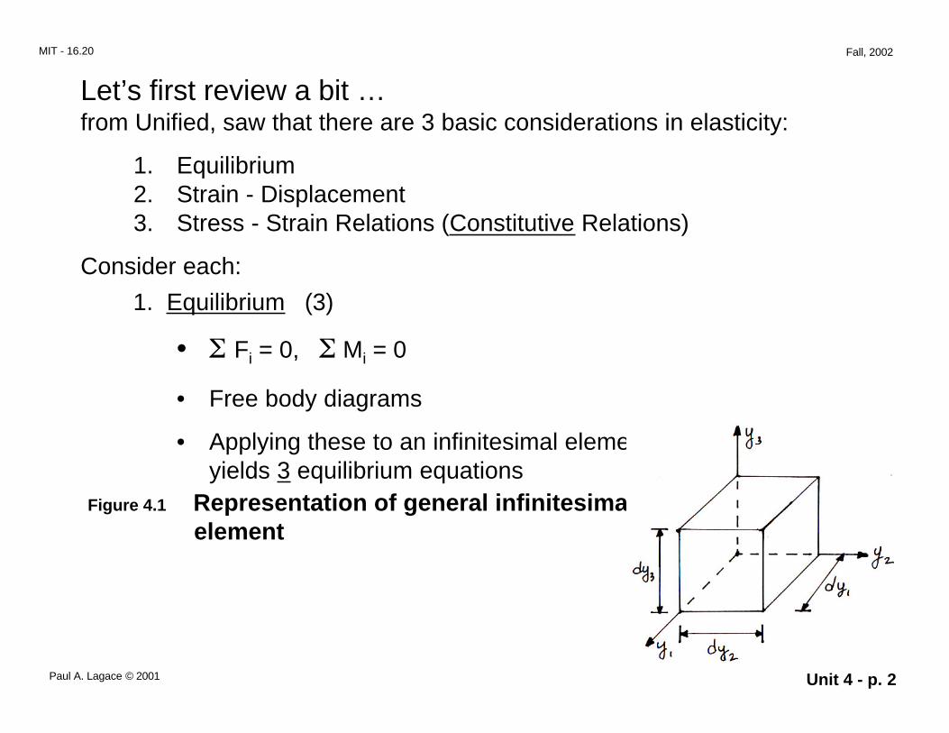
• Applying these to an infinitesimal element yields 3 equilibrium equations

Figure 4.1 Representation of general infinitesimal element

Paul A. Lagace © 2001 Unit 4 - p. 2

MIT - 16.20 Fall, 2002

∂σ11 + ∂σ21 +

∂σ31 + f1 = 0 (4-1) ∂y1 ∂y2 ∂y3 ∂σ12 +

∂σ22 + ∂σ32 + f2 = 0 (4-2)

∂y1 ∂y2 ∂y3 ∂σ13 +

∂σ23 + ∂σ33 + f3 = 0 (4-3)

∂y1 ∂y2 ∂y3

∂∂

+ σmn

m n yf 0 =

2. Strain - Displacement (6)

• Based on geometric considerations

• Linear considerations (I.e., small strains only -- we will talk about

large strains later) (and infinitesimal displacements only)

Paul A. Lagace © 2001 Unit 4 - p. 3

MIT - 16.20 Fall, 2002

ε11 =∂u1 (4-4)∂y1

ε22 =∂u2 (4-5)∂y2

ε33 =∂u3 (4-6)∂y3

ε21 = ε12 = 1

∂u1 +

∂u2

2 ∂y2 ∂y1

ε31 = ε13 =1

∂u1 +

∂u3

2 ∂y3 ∂y1

ε32 = ε23 =1

∂u2 +

∂u3

2 ∂y3 ∂y2

(4-7)

(4-8)

(4-9)

1 ∂um + ∂un

εmn =

2 ∂yn ∂ym

Paul A. Lagace © 2001 Unit 4 - p. 4

MIT - 16.20 Fall, 2002

3. Stress - Strain (6)

σmn = Emnpq εpq

we’ll come back to this …

Let’s review the “4th important concept”: Static Determinance

There are there possibilities (as noted in U.E.)

a. A structure is not sufficiently restrained (fewer reactions than d.o.f.)

degrees of freedom

⇒ DYNAMICS

b. Structure is exactly (or “simply”) restrained (# of reactions = # of d.o.f.)

⇒ STATICS (statically determinate)

Implication: can calculate stresses via equilibrium (as done in Unified)

Paul A. Lagace © 2001 Unit 4 - p. 5

MIT - 16.20 Fall, 2002

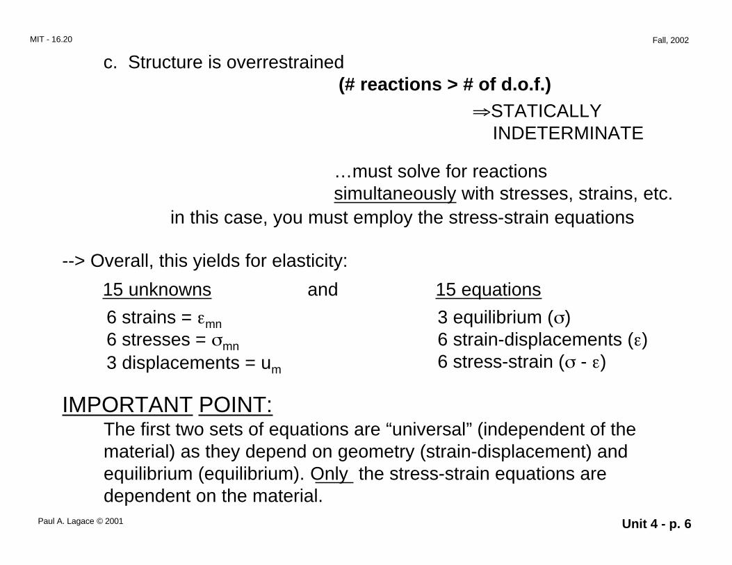
c. Structure is overrestrained (# reactions > # of d.o.f.)

⇒STATICALLY INDETERMINATE

…must solve for reactions simultaneously with stresses, strains, etc.

in this case, you must employ the stress-strain equations

--> Overall, this yields for elasticity:

15 unknowns and 15 equations

6 strains = εmn 3 equilibrium (σ) 6 stresses = σmn 6 strain-displacements (ε) 3 displacements = um 6 stress-strain (σ - ε)

IMPORTANT POINT: The first two sets of equations are “universal” (independent of the material) as they depend on geometry (strain-displacement) and equilibrium (equilibrium). Only the stress-strain equations are dependent on the material.

Paul A. Lagace © 2001 Unit 4 - p. 6

∂ ∂ ∂ ∂

MIT - 16.20 Fall, 2002

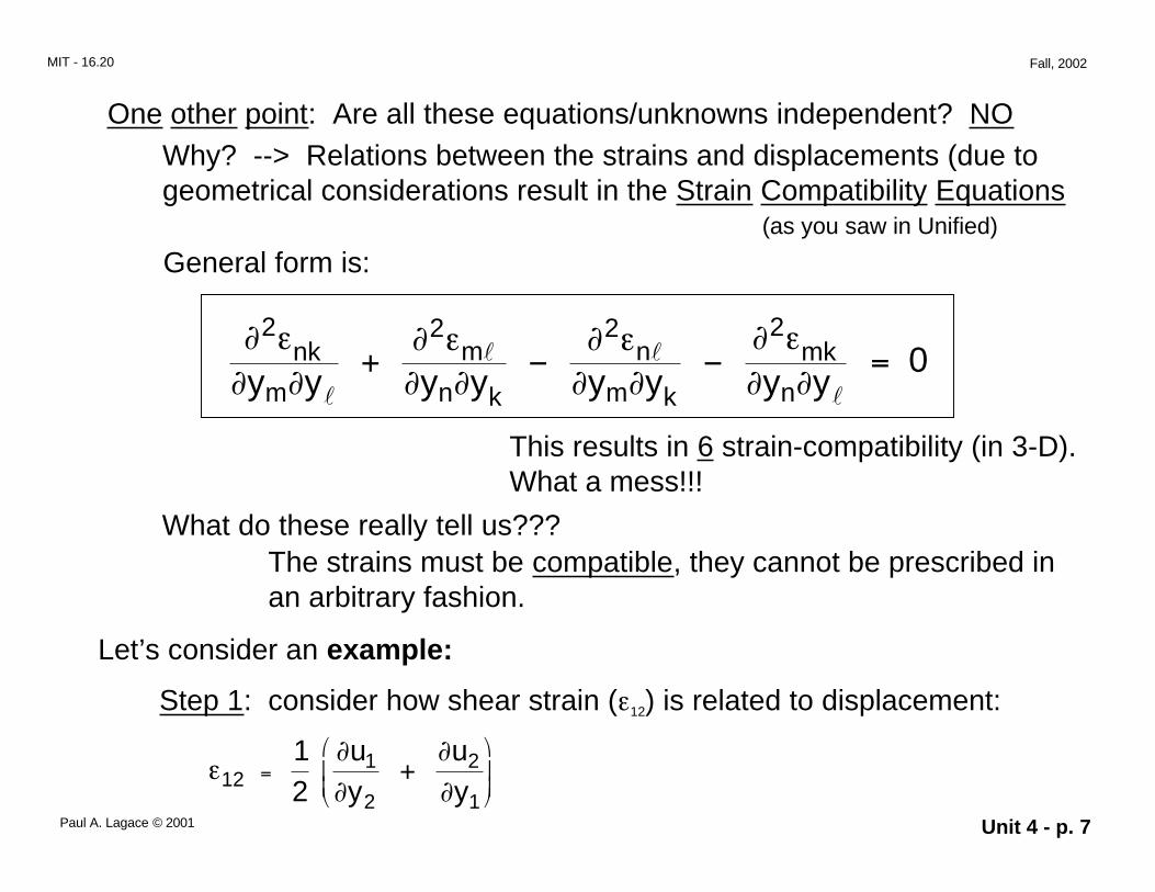
One other point: Are all these equations/unknowns independent? NO Why? --> Relations between the strains and displacements (due to geometrical considerations result in the Strain Compatibility Equations

(as you saw in Unified)

General form is:

∂2εnk + ∂2εml −

∂2εnl −∂2εmk = 0

y yl ∂ ∂yk y yk ∂ ∂ylm yn m yn

This results in 6 strain-compatibility (in 3-D). What a mess!!!

What do these really tell us??? The strains must be compatible, they cannot be prescribed in an arbitrary fashion.

Let’s consider an example:

Step 1: consider how shear strain (ε12) is related to displacement:

1 ∂u1 ∂u2

+ ε12 = 2 ∂y2 ∂y1

Paul A. Lagace © 2001 Unit 4 - p. 7

∂ ∂ ∂ ∂ ∂ ∂

MIT - 16.20 Fall, 2002

Note that deformations (um) must be continuous single-valued functions for continuity. (or it doesn’t make physical sense!)

Step 2: Now consider the case where there are gradients in the strain field

∂ε12 ≠ 0, ∂ε12 ≠ 0

∂y1 ∂y2

This is the most general case and most likely in a general structure

Take derivatives on both sides:

∂2ε12 1 ∂3u1 ∂3u2 ⇒ = 2 + 2y y2 2 y y2 y y2

1 1 1

Step 3: rearrange slightly and recall other strain-displacement equations

∂u1 = ε1 , ∂u2 ε2 =

∂y1 ∂y2

Paul A. Lagace © 2001 Unit 4 - p. 8

∂ ∂

MIT - 16.20 Fall, 2002

∂2ε12 1 ∂2ε11 + ∂2ε22 ⇒ = 2y y2 2 ∂y2 ∂y1

2 1

So, the gradients in strain are related in certain ways since they are all related to the 3 displacements.

Same for other 5 cases …

Let’s now go back and spend time with the …

Stress-Strain Relations and the Elasticity Tensor

In Unified, you saw particular examples of this, but we now want to generalize it to encompass all cases.

The basic relation between force and displacement (recall 8.01) is Hooke’s Law:

F = kx

spring constant (linear case)

Paul A. Lagace © 2001 Unit 4 - p. 9

MIT - 16.20 Fall, 2002

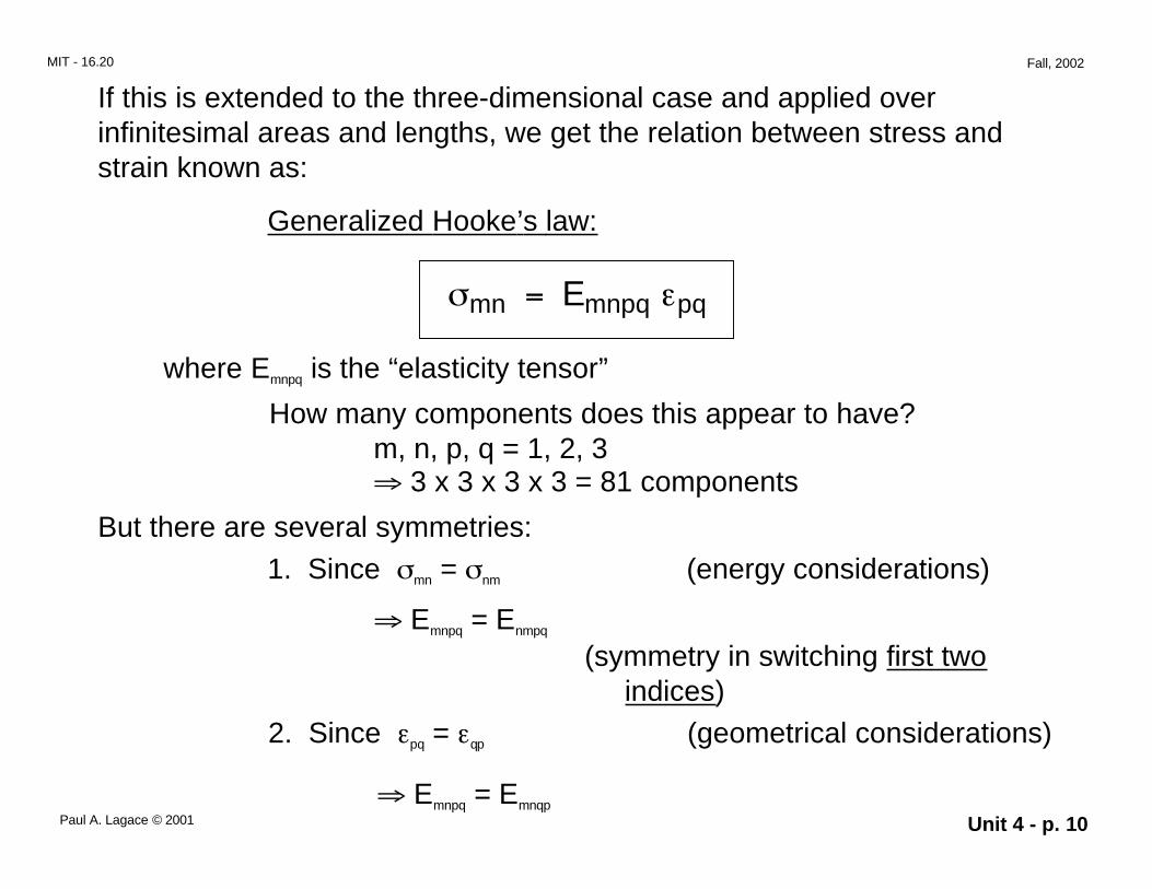
If this is extended to the three-dimensional case and applied over infinitesimal areas and lengths, we get the relation between stress and strain known as:

Generalized Hooke’s law:

σmn = Emnpq εpq

where Emnpq is the “elasticity tensor”

How many components does this appear to have? m, n, p, q = 1, 2, 3 ⇒ 3 x 3 x 3 x 3 = 81 components

But there are several symmetries:

1. Since σmn = σnm (energy considerations)

⇒ Emnpq = Enmpq

(symmetry in switching first two indices)

2. Since εpq = εqp (geometrical considerations)

⇒ Emnpq = Emnqp Paul A. Lagace © 2001 Unit 4 - p. 10

2212

MIT - 16.20 Fall, 2002

(symmetry in switching last two indices)

3. From thermodynamic considerations (1st law of thermo)

⇒ Emnpq = Epqmn

(symmetry in switching pairs of indices)

Also note that: Since σmn = σnm

are only 6! , the apparent 9 equations for stress

With these symmetrics, the resulting equations are:

σ11 E1111 E1122 E1133 2E1123 2E1113 2E1112 ε11

E1122 E2222 E2233 2E2223 2E2213 2E2212

ε22 σ22 σ33 E1133 E2233 E3333 2E3323 2E3313 2E3312 ε33 = σ23 E1123 E2223 E3323 2E2323 2E1323 2E1223

ε23 σ13 E1113 E2213 E3313 2E1323 2E1313 2E1213 ε13 σ12 E1112 E2212 E3312 2E1223 2E1213 2E1212 ε12

Paul A. Lagace © 2001 Unit 4 - p. 11

MIT - 16.20 Fall, 2002

Results in 21 independent components of the elasticity tensor • Along diagonal (6) • Upper right half of matrix (15)

[don’t worry about 2’s]

Also note: 2’s come out automatically…don’t put them in ε~ For example: σ12 = … E1212 ε12 + E1221 ε21 …

= … 2E1212 ε12 …

These Emnpq can be placed into 3 groups:

• Extensional strains to extensional stresses E1111 E1122

E2222 E1133

E3333 E2233

e.g., σ11 = … E1122 ε22 …

• Shear strains to shear stresses E1212 E1213

E1313 E1323

E2323 E2312

Paul A. Lagace © 2001 Unit 4 - p. 12

MIT - 16.20 Fall, 2002

e.g., σ12 = … 2E1223 ε23 …

• Coupling term: extensional strains to shear stress or shear strains to extensional stresses

E1112 E2212 E3312

E1113 E2213 E3313

E1123 E2223 E3323

e.g., σ12 = …E1211 ε11… 11 = …2E1123 ε23…σ

A material which behaves in this manner is “fully” anisotropic

However, there are currently no useful engineering materials which have 21 different and independent components of Emnpq

The “type” of material (with regard to elastic behavior) dictates the number of independent components of Emnpq:

Paul A. Lagace © 2001 Unit 4 - p. 13

MIT - 16.20 Fall, 2002

2Isotropic

3Cubic

5“Transversely Isotropic”*

6Tetragonal

9Orthotropic

13Monoclinic

21Anisotropic

# of Independent Components of Emnpq

Material Type

Useful Engineering

Materials

Composite Laminates

Basic Composite

Ply

Metals (on average)

Good Reference: BMP, Ch. 7*not in BMP

For orthotropic materials (which is as complicated as we usually get), there are no coupling terms in the principal axes of the material

Paul A. Lagace © 2001 Unit 4 - p. 14

MIT - 16.20 Fall, 2002

• When you apply an extensional stress, no shear strains arise e.g., E1112 = 0

(total of 9 terms are now zero)

• When you apply a shear stress, no extensional strains arise (some terms become zero as for

previous condition)

• Shear strains (stresses) in one plane do not cause shear strains (stresses) in another plane

( E1223 , E1213 , E1323 = 0)

With these additional terms zero, we end up with 9 independent components:

(21 - 9 - 3 = 9)

and the equations are:

Paul A. Lagace © 2001 Unit 4 - p. 15

⇒⇒⇒

13

MIT - 16.20 Fall, 2002

σ11 E1111 E1122 E1133 0 0 0 ε11

E1122 E2222 E2233 0 0 0

σ22

ε22 σ33 E1133 E2233 E3333 0 0 0 ε33 = σ23

0 0 0 2E2323 0 0 ε23 σ13 0 0 0 0 2E1313 0 ε13 σ12

0 0 0 0 0 2E1212 ε12

For other cases, no more terms become zero, but the terms are not Independent.

For example, for isotropic materials:

• E1111 = E2222 = E3333

• E1122 = E1133 = E2233

• E2323 = E1313 = E1212

• And there is one other equation relating E1111 , E1122 and E2323

⇒ 2 independent components of Emnpq

(we’ll see this more when we do engineering constants)

Paul A. Lagace © 2001 Unit 4 - p. 16

MIT - 16.20 Fall, 2002

Why, then, do we bother with anisotropy? Two reasons: 1. Someday, we may have useful fully anisotropic materials

(certain crystals now behave that way) Also, 40-50 years ago, people only worried about isotropy

2. It may not always be convenient to describe a structure (i.e., write the governing equations) along the principal material axes.

How else? Loading axes

Examples

Figure 4-2

wing

rocket case fuselage

Paul A. Lagace © 2001 Unit 4 - p. 17

MIT - 16.20 Fall, 2002

In these other axis systems, the material may have “more” elastic components. But it really doesn’t.

(you can’t “create” elastic components just by describing a material in a different axis system, the inherent properties of the material stay the same).

Figure 4-3 Example: Unidirectional composite (transversely isotropic)

No shear / extension coupling Shears with regard to loading axis but still no inherent shear/extension coupling

In order to describe full behavior, need to do …TRANSFORMATIONS

(we’ll review this/expand on it later)

Paul A. Lagace © 2001 Unit 4 - p. 18

MIT - 16.20 Fall, 2002

--> It is often useful to consider the relationship between stress and strain (opposite way). For this we use

COMPLIANCE

εmn = Smnpq σpq

where: Smnpq = compliance tensor

Paul A. Lagace © 2001 Unit 4 - p. 19

MIT - 16.20 Fall, 2002

Using matrix notation: σ = E ε ~ ~ ~ and E-1 σ ~~ = ε ~

inverse

with ε = S σ~ ~ ~ this means

E-1 = S~ ~

⇒ E S = I~ ~ ~ ⇒The compliance matrix is the

inverse of the elasticity matrix

Note: the same symmetries apply to Smnpq as to Emnpq

Paul A. Lagace © 2001 Unit 4 - p. 20

MIT - 16.20 Fall, 2002

Meaning of each:

• Elasticity term Emnpq: amount of stress (σmn) related to the deformation/strain (εpq)

• Compliance term Smnpq: amount of strain (εmn) the stress (σpq) causes

These are useful in defining/ determining the “engineering constants”

All of this presentation on elasticity (and what you had in

Unified) is based on assumptions which limit their applicability:

which we will review / introduce / expand on in the next lecture.

CAUTION

• Small strain • Small displacement / infinitesimal (linear) strain

Fortunately, most engineering structures are such that these assumptions cause negligible error.

Paul A. Lagace © 2001 Unit 4 - p. 21

MIT - 16.20 Fall, 2002

However, there are cases where this is not true: • Manufacturing (important to be able to convince) • Compliant materials • Structural examples: dirigibles, …

So let’s explore:

Large strain and the formal definition of strain

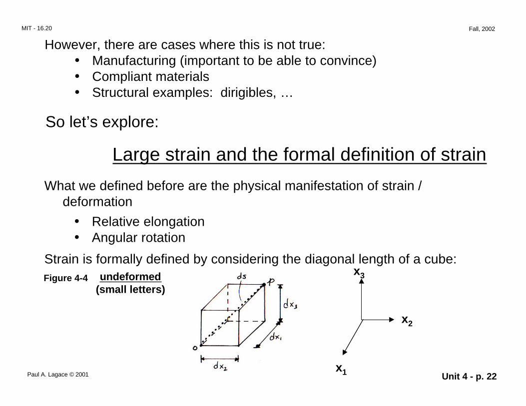
What we defined before are the physical manifestation of strain / deformation

• Relative elongation • Angular rotation

Strain is formally defined by considering the diagonal length of a cube: Figure 4-4 undeformed x3

(small letters)

x2

Paul A. Lagace © 2001 x1 Unit 4 - p. 22

MIT - 16.20 Fall, 2002

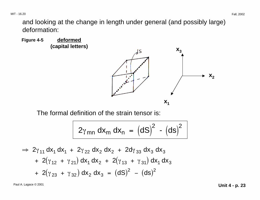
and looking at the change in length under general (and possibly large) deformation:

Figure 4-5 deformed (capital letters) x3

x2

x1

The formal definition of the strain tensor is:

2 22γ mn dxm dxn = (dS) - (ds)

⇒ 2γ 11 dx1 dx1 + 2γ 22 dx2 dx2 + 2dγ 33 dx3 dx3

+ 2(γ 12 + γ 21) dx1 dx2 + 2(γ 13 + γ 31) dx1 dx3

2 2+ 2(γ 23 + γ 32 ) dx2 dx3 = (dS) − (ds) Paul A. Lagace © 2001 Unit 4 - p. 23

MIT - 16.20 Fall, 2002

where γmn = formal strain tensor.

This is a definition. The physical interpretation is related to this but not directly in the general case.

One can show (see BMP 5.1 - 5.4) that the formal strain tensor is related to relative elongation (the familiar ∆l ) via:

l

relative elongation in m-direction:

Em = m1 γ m+ 2 − 1 (no summation on m)

and is related to angular change via: 2γ mnsin φ = mn (1 + Em ) (1 + En )

Thus, it also involves the relative elongations!

Most structural cases deal with relatively small strain. If the relative elongation is small (<<100%)

⇒ Em <<1

Paul A. Lagace © 2001 Unit 4 - p. 24

MIT - 16.20 Fall, 2002

look at: Em = 1 + 2γ mm − 1

2 ⇒ (Em + 1) = 1 + 2γ mm

E2 + 2Em = 2γ mmm

but if Em << 1, then E2m ≈ 0

⇒ Em = γmm

Relative elongation = strain ∆l = ε small strain approximation!l

Can assess this effect by comparing 2Em and Em (2 + Em)

relative elongation = Em

2Em Em (2 + Em) % error

0.01 0.02 0.0201 0.5% 0.02 0.04 0.0404 1.0% 0.05 0.10 0.1025 2.4% 0.10 0.20 0.2100 4.8%

Paul A. Lagace © 2001 Unit 4 - p. 25

MIT - 16.20 Fall, 2002

Similarly, consider the general expression for rotation: 2γ mnsin φ = mn (1 + Em ) (1 + En )

for small elongations (Em << 1, En << 1) ⇒ sin φmn = 2γ mn

and, if the rotation is small:

sin φmn ≈ φmn

⇒ φmn = 2γ mn

= 2εmn small strain approximation! (as before)

Note: factor of 2 !

Even for a balloon, the small strain approximation may be good enough

So: from now on, small strain assumed, but • understand limitations • be prepared to deal with large strain • know difference between formal definition and the engineering

approximation which relates directly to physical reality. Paul A. Lagace © 2001 Unit 4 - p. 26

MIT - 16.20 Fall, 2002

What is the other limitation? It deals with displacement, so consider

Large Displacement and Non-Infinitesimal (Non-linear) Strain

See BMP 5.8 and 5.9 The general strain-displacement relation is:

1 ∂u ∂u ∂u ∂u γ mn =

m + n + r s δrs 2 ∂xn ∂xm ∂xm ∂xn

Where: δrs = Kronecker delta

The latter terms are important for larger displacements but are higher order for small displacements and can then be ignored to arrive back at:

1 ∂um + ∂un

εmn =

2 ∂yn ∂ym

Paul A. Lagace © 2001 Unit 4 - p. 27

MIT - 16.20 Fall, 2002

How to assess?

Look at ∂um ∂ur ∂usvs. δrs∂xn ∂xm ∂xn

and compare magnitudes

Small vs. large and linear vs. nonlinear will depend on:

• material(s) • structural configuration • mode of behavior • the loading

Examples

• Rubber in inflated structures ⇒ Large strain (Note: generally means larger displacement)

• Diving board of plastic or wood ⇒ Small strain but possibly large displacement (will look at this

more when we deal with beams)

Paul A. Lagace © 2001 Unit 4 - p. 28

MIT - 16.20 Fall, 2002

• Floor beam of steel ⇒ Small strain and linear strain (Note: linear strain must also be ⇒ small)

Next…back to constitutive constants…now their physical reality

Paul A. Lagace © 2001 Unit 4 - p. 29