Page 1
University of Texas at El PasoDigitalCommons@UTEP
Open Access Theses & Dissertations
2014-01-01
Equations of State in a Strongly InteractingRelativistic SystemJason Paul KeithUniversity of Texas at El Paso, [email protected]
Follow this and additional works at: https://digitalcommons.utep.edu/open_etdPart of the Physics Commons
This is brought to you for free and open access by DigitalCommons@UTEP. It has been accepted for inclusion in Open Access Theses & Dissertationsby an authorized administrator of DigitalCommons@UTEP. For more information, please contact [email protected] .
Recommended CitationKeith, Jason Paul, "Equations of State in a Strongly Interacting Relativistic System" (2014). Open Access Theses & Dissertations. 1272.https://digitalcommons.utep.edu/open_etd/1272
Page 2
EQUATIONS OF STATE IN A STRONGLY INTERACTING RELATIVISTIC SYSTEM
Jason P. Keith
Department of Physics
APPROVED:
Efrain Ferrer, Chair, Ph.D.
Vivian de la Incera, Ph.D.
Piotr Wojciechowski, Ph.D.
Juan Noveron, Ph.D.
Bess Sirmon-Taylor, Ph.D.
Interim Dean of the Graduate School
Page 3
EQUATIONS OF STATE IN A STRONGLY INTERACTING RELATIVISTIC SYSTEM
by
Jason P. Keith
THESIS
Presented to the Faculty of the Graduate School of
The University of Texas at El Paso
in Partial Fulfillment
of the Requirements
for the Degree of
MASTER OF SCIENCE
Department of Physics
THE UNIVERSITY OF TEXAS AT EL PASO
August 2014
Page 4
Acknowledgements
This work was conducted under the advisement of Dr. E.J. Ferrer at the University of Texas
at El Paso, and has been supported by the UTEP-COURI-2011 grant and DOE Nuclear
Theory grant de-sc0002179. Special thanks to Israel Portillo for advice on computational
methods, Vivian de la Incera, and the rest of the high-energy theory group.
iii
Page 5
Abstract
It has long been understood that the ground state of a superdense quark system, a Fermi
liquid of weakly interacting quarks, is unstable with respect to the formation of diquark
condensates. This nonperturbative phenomenon is essentially equivalent to the Cooper in-
stability of conventional BCS superconductivity. As the quark pairs have nonzero color
charge, this kind of superconductivity breaks the SU(3) color gauge symmetry, thus the phe-
nomenon is called color superconductivity. However, not much is known about the behavior
of quark systems at moderate densities between the formation of baryons and asymptotic
freedom. Strong theoretical and experimental evidence suggests that there will be a smooth
crossover between the two, during which the color superconducting properties of the quark
system will undergo a shift between dynamics of a Bose-Einstein condensate (BEC) and
weakly bound diquark pairs governed by BCS theory. Chromomagnetic instabilities exist for
the densities in question and it is unclear what phase will resolve them. Therefore, there are
many different proposed models accounting for several possible phases in need of thorough
investigation. The analysis of two simple models that exhibit the crossover between a BCS
state and a Bose-Einstein Condensate (BEC), as well as the evolution of the corresponding
equation of state through the crossover, are the topics of this thesis.
iv
Page 6
Table of Contents
Page
Acknowledgements . . . . . . . . . . . . . . . . . . . . . . . . . . . . . . . . . . . . . iii
Abstract . . . . . . . . . . . . . . . . . . . . . . . . . . . . . . . . . . . . . . . . . . . iv
Table of Contents . . . . . . . . . . . . . . . . . . . . . . . . . . . . . . . . . . . . . . v
List of Figures . . . . . . . . . . . . . . . . . . . . . . . . . . . . . . . . . . . . . . . vii
List of Figures . . . . . . . . . . . . . . . . . . . . . . . . . . . . . . . . . . . . . . vii
1 Introduction . . . . . . . . . . . . . . . . . . . . . . . . . . . . . . . . . . . . . . . 1
1.1 Objectives of Thesis . . . . . . . . . . . . . . . . . . . . . . . . . . . . . . . 4
2 Theoretical Background . . . . . . . . . . . . . . . . . . . . . . . . . . . . . . . . 5
2.1 Equations of State and Thermodynamic Potentials . . . . . . . . . . . . . . 5
2.2 Superconductivity . . . . . . . . . . . . . . . . . . . . . . . . . . . . . . . . . 7
2.3 QCD . . . . . . . . . . . . . . . . . . . . . . . . . . . . . . . . . . . . . . . . 9
2.4 QCD Phase Diagram . . . . . . . . . . . . . . . . . . . . . . . . . . . . . . . 10
2.5 BCS-BEC crossover . . . . . . . . . . . . . . . . . . . . . . . . . . . . . . . . 12
2.6 Newton’s Method . . . . . . . . . . . . . . . . . . . . . . . . . . . . . . . . . 13
3 Equations of State in a Relativistic Boson-Fermion System . . . . . . . . . . . . . 15
3.1 Composite-Boson-Fermion model . . . . . . . . . . . . . . . . . . . . . . . . 15
3.2 Gap Equation at Fixed Fermion Density . . . . . . . . . . . . . . . . . . . . 18
3.3 Numerical Solutions . . . . . . . . . . . . . . . . . . . . . . . . . . . . . . . . 18
4 Fermionic Model for a Relativistic Superfluid . . . . . . . . . . . . . . . . . . . . . 23
4.1 Purely-Fermionic model . . . . . . . . . . . . . . . . . . . . . . . . . . . . . 23
4.2 Numerical solutions . . . . . . . . . . . . . . . . . . . . . . . . . . . . . . . . 25
4.3 Stability Condition in the BEC Region . . . . . . . . . . . . . . . . . . . . . 26
5 Final Remarks . . . . . . . . . . . . . . . . . . . . . . . . . . . . . . . . . . . . . 29
References . . . . . . . . . . . . . . . . . . . . . . . . . . . . . . . . . . . . . . . . . . 31
v
Page 7
Curriculum Vitae . . . . . . . . . . . . . . . . . . . . . . . . . . . . . . . . . . . . . . 35
vi
Page 8
List of Figures
2.1 QCD Phase Diagram . . . . . . . . . . . . . . . . . . . . . . . . . . . . . . . 11
3.1 Chemical potential and energy in composite boson model . . . . . . . . . . . 19
3.2 Quasiparticle dispersion curves in composite boson model . . . . . . . . . . . 19
3.3 Boson and fermion densities in composite boson model . . . . . . . . . . . . 20
3.4 Pressure and energy in composite boson model . . . . . . . . . . . . . . . . . 21
4.1 Chemical potential in fermionic model . . . . . . . . . . . . . . . . . . . . . 24
4.2 Energy gap in fermionic model . . . . . . . . . . . . . . . . . . . . . . . . . . 25
4.3 Dispersion curves in fermionic model . . . . . . . . . . . . . . . . . . . . . . 27
4.4 Pressure in fermionic model . . . . . . . . . . . . . . . . . . . . . . . . . . . 28
vii
Page 9
Chapter 1
Introduction
The strong nuclear interaction is one of the four fundamental interactions of nature. Gov-
erned by quantum chromodynamics (QCD) it provides a description of how nucleons (pro-
tons and neutrons) stay bound together in a nucleus via their constituent particles, known as
quarks, which couple with the strong force. Quarks are fundamental particles, classified as
fermions, spin-1/2 particles, which are predicted to exist by the Standard Model of particle
physics. Quarks couple to the strong nuclear interaction which, unlike the electromagnetic
interaction, has three different charges called colors. Quarks also come in several different
species. The three species relevant to the current topic are up (u), down (d), and strange (s),
this introduces a new degree of freedom referred to as flavor. Although individual quarks
have never been observed in a lab, one possible explanation for this lack of observational evi-
dence could be attributed to the nature of the strong interaction whose coupling constant, or
strength of the interaction, increases as distance increases between the interacting particles,
meaning that separating them requires increasing amounts of energy. On the other hand,
at very small distance their interaction becomes negligibly small. That is, very energetic
quarks that can be very close do not interact. This is what is called the asymptotic freedom
of the strong interaction. It is thought that under extreme temperature and negligible pres-
sures, quarks may experience deconfinement and overcome the strong attraction to become
unbound free particles. Interestingly, that is not the only way in which quarks might act as
free particles considering that if, rather than providing enough energy to liberate them, one
were to compress the hadrons decreasing the average separation of their consituent quarks,
this would decrease the coupling strength to arbitrarily low values. The boundaries of previ-
ously distinct hadrons then overlap leaving only a dense fermion gas of approximately freely
1
Page 10
moving fermions in asymptotic freedom.
Asymptotic freedom was first described in 1973 by David Gross, Frank Wilczek, and
David Politzer [1] for which they shared a Nobel prize in 2004. When asymptotic freedom
occurs the quarks may be thought of approximately as free particles.
The immense pressure and relatively low temperatures that can be found within the cores
of dense neutron stars might provide adequate conditions for asymptotic freedom to mani-
fest. Because fermions are subject to the Pauli exclusion principle (discussed in section 2.3)
they populate all energy states up to the Fermi-surface. The physics of a weakly interacting
system such as this, is already well described in the context of superconductivity of electrons
within a framework known as BCS theory (named after its creators Bardeen, Cooper, and
Schreifer), in which the electrons experience an attractive potential due to phonon interac-
tions allowing them to form bound states of two electrons with opposite spins called Cooper
pairs. This framework can readily be applied to the context of cold asymptotically free
quarks as well since the Cooper instability described by the theory applies to any fermionic
system with an attractive interaction at sufficiently low temperature. These conditions suit
color superconductivity well due to quark interactions in QCD possessing attractive chan-
nels. The theory resolves the instability with the creation of Cooper pairs, two quarks with
opposite momentum and spin bound together by their weak attraction, resulting in a gap for
the energy required to create a particle at the Fermi surface such that no excitation energies
exist with vanishing free energy. The formed state of matter is known as a color supercon-
ductor, where the term color comes from the fact that the ground state is now charged with
respect to the color charge.
In temperature versus chemical potential plane of the QCD phase diagram the region
of asymptotically large µ and zero T is well understood in the context of weakly coupled
QCD, in which all the quarks are paired in diquarks in the energetically favored Color-
Flavor-Locked (CFL) superconducting phase. The CFL phase is characterized by a zero
spin diquark condensate which is antisymmetric in both color and flavor. Besides looking for
signatures of color superconductivity in neutron stars there are experiments planned which
2
Page 11
could possibly probe color superconductivity in the future at locations such as the Facility
for Antiproton and Ion Research (FAIR) at GSI, the Nuclotron-Ion Collider Facility (NICA)
at JINR, the Japan Proton Accelerator Research Complex (JPARK) at JAERI, Brookhaven
National Lab (BNL) at RHIC, and CERN at the LHC [25].
Chiral models of QCD, which take the limit as the fermion mass tends to zero, predict
critical points in the QCD phase diagram (shown in Section 2.4) implying that beneath the
relevant critical point might lie a region in which hadronic matter is capable of smoothly
transitioning into a color superconductor rather than undergoing a phase transition. This
smooth transition is called a crossover.
It is thought that in smoothly fine tuning the diquark coupling strength, which might be
thought of as increasing as the radial distance decreases to the center of the neutron star,
the Fermi gas gives rise to a regime where the fermions are bound into states of quark pairs
with all combinations of colors and flavors in the so called Color-Flavor-Locked (CFL) phase
[11]. These pairs would then comprise of a composite boson, which is no longer subject to
the Pauli exclusion principle, which at such low temperatures would correspond to a Bose-
Einstein-condensate (BEC) and might still retain its color superconducting properties due
to the fact that the ground state is now color charged.
Decreasing the density it was found that there exists chromomagnetic instabilities, which
are exhibited as a consequence of mismatched Fermi momenta of different quarks produced
by the strange quark mass ms together with the constraints imposed by electric and color
neutralities. Due to such instabilities it is unclear what phase is most stable for a color
superconductor at intermediate densities as those between hadronic matter and color super-
conducting CFL phase at high density. Therefore, exploratory work is being done in this
area to remove the chromomagnetic instabilities [26]. Several interesting models have been
proposed, such as a CFL-phase modified to include a kaon condensate [27], a LOFF phase
on which the quarks pair with nonzero total momentum [28], and an inhomogeneous gluon
condensate [29]. To obtain deeper insight into the nature of the unknown stable phase is the
motivation of our research.
3
Page 12
1.1 Objectives of Thesis
The objective of this thesis is to present an overview of the physics and recent developments
surrounding the smooth crossover, described above, in the dynamics of color superconductors
between BCS and BEC descriptions. We will consider two simplified toy models to investigate
the BCS-BEC crossover and analyze its impact in the systems’ equations of state (EoS).
The results and conclusions presented here are, therefore, not definitive within the overall
framework of QCD but serve to provide deeper insight toward that goal. The Lagrangians
of each respective model will allow calculation of thermodynamic potentials, which will be
set to zero temperature as is the limit for the states of matter, which are most interesting
for astrophysical applications. One of the models in question will contain both bosonic and
fermionic degrees of freedom, which are treated as separate degrees of freedom, and a second
model describing a simple four fermion interaction in which only fermionic degrees of freedom
exist, but its bosonic behavior is realized through the formation of diquarks. We then can
take the difermion coupling strength to act as a crossover parameter to drive the system
between higher and lower density regions, effectively moving between the domains of BCS
and BEC dynamics smoothly. In doing this, we will observe similar implications for the
stability of the star within both models.
The thesis will be organized as follows: Chapter 2 will serve to introduce the necessary
formalism and the theoretical background used in later chapters. In Chapter 3 we introduce
a simple model for the crossover in which the system is taken to possess fermionic and
bosonic degrees of freedom. Chapter 4 then presents a second model with only fermionic
degrees of freedom, where the crossover occurs via a shift between the nature of the system
quasiparticles at some critical value of the diquark attractive coupling. Finally, in Chapter
5 we conclude with a general discussion of the obtained results, a comparison between the
two models, and an outlook of needed future investigagions.
4
Page 13
Chapter 2
Theoretical Background
2.1 Equations of State and Thermodynamic Potentials
Equations of state are relations between dynamical state variables that can include any of
the following: temperature T , entropy S, pressure p, volume V , chemical potential µ, and
particle number N . The last two can be defined for each species of particle in the system.
One is able to find relations between these variables by the use of the thermodynamic
potentials, originally formulated in 1886 by Pierre Duhem. A different thermodyanmic po-
tential exists for each combination formed by making each of the above variables either
dyanamic or constant. Once one thermodynamic potential is known the others may be
found by taking Legendre transformations of it, typically done with the internal energy U
due to U having a well understood physical interpretation.
The particular thermodynamic potential which is of interest to us in the rest of the
discussions to follow is the Grand potential Ω, and so all reference to the term thermodynamic
potential will be used interchangeably with Grand potential beyond this section. The Grand
potential has the following definition
Ω = U − TS −∑i
µiNi. (2.1)
The quantity U can be found from considerations of the system available energy mi-
crostates, and this is done via a factor known as the partition function, which is simply the
5
Page 14
sum of Boltzmann factors over all energy states [8]
Z(T ) =∑s
exp(−εs/kBT ) (2.2)
where kB is Boltzmann’s constant and εs is the energy of state s. In Quantum Field Theory
(QFT) it is given instead by the path integral on field configurations
Z =
∫D[φ]exp
(i
∫d4k
(2π)4φ(−k)G−1(k)φ(k)
)(2.3)
where G−1(k) is the inverse field propagator.
One can verify that
Ω = −T lnZ (2.4)
is a solution to Eq (2.1) by also noting that
S = −(∂Ω
∂T
)V,µi
Ni = −(∂Ω
∂µi
)T,V,µj 6=i
, (2.5)
where the notation being used in the derivative subscripts is a list of variables being held
constant for the partial derivative.
It will now be useful to define here the total derivative of the grand potential, which
comes directly from Eq (2.1) and the total derivative of U
dU = TdS − pdV −∑i
µidNi, (2.6)
which may be arranged into
d(U − TS −∑i
µiNi) = −SdT − pdV −∑i
Nidµi = dΩ. (2.7)
From Eq (2.7) we can now define the system pressure, which will be useful in later
sections. One sees that in finding the partial derivative of the thermodynamic potential with
6
Page 15
respect to volumedΩ
dV= −S dT
dV− p−
∑i
NidµidV
, (2.8)
and by holding temperature and chemical potential constant, this leads to our definition for
the pressure being
p = −(∂Ω
∂V
)T,µi
, (2.9)
and the definition for particle number
Ni = −(∂Ω
∂µi
)T,V,µj 6=i
, (2.10)
which is akin to the particle density that will be used in later sections. Following a similar
procedure used in deriving Eq (2.7) one can define
F = Ω +∑i
µiNi (2.11)
which gives the free energy of the system.
2.2 Superconductivity
The first scientific observation of superconducting phenomena was made by Heike Kamer-
lingh Onnes in 1911 [2]. He observed that at extremely low temperatures, below a certain
threshhold temperature, which depends on the conductors material, a current is able to
flow without any resistance. However, this could be imagined as simply a perfect conductor,
which was Onnes’ motivation for studying the phenomenon. He was attempting to determine
if the resistivity would vanish according to the Drude model, or whether it would actually
increase as proposed by Lord Kelvin. Unexpectedly, however the resistance did not gradually
drop but did so suddenly, hinting that this may be a new phenomenon at work. Onnes won
the Nobel prize in 1913 for this research that led to the creation of liquid helium. However,
7
Page 16
it wasn’t until the discovery (of the so called Meissner effect) by Meissner and Ochsenfeld in
1933 [22], a complete expulsion of a magnetic field from the superconductor as its temper-
ature drops below the critical value TC , that physicsts realized a completely new theory of
superconductivity would be required.
In any idealized perfect conductor an external magnetic field would be repelled by the
simple creation of currents on its surface, which do not diminish in time due to zero resistance.
These currents would generate an induced magnetic field that would completely oppose
any external magnetic field. However, this is not, in general, the behaviour observed in
superconductors. As stated above, the expulsion of the magnetic field inside the conductor,
up to a distance from the surface known as the London penetration depth, by an opposing
one is set up at the moment the superconductor drops below the threshhold temperature and
bemes a superconductor. This induced magnetic field is permanent and does not account
for any new changes in external magnetic fields, and therefore the currents set up at the
creation of the superconductor are known as persistent currents.
A microscopic theory of superconductivity, known as BCS theory after its creators Bardeen,
Cooper, and Schrieffer, was published in 1957 for which they shared a Nobel prize. A normal
superconductor allows electrical current to flow through it with no resistance. This occurs
because vibrations of the lattice, mediated by phonons, can give rise to a net attractive force
between electrons that are relatively far apart. The resulting bound state is called a Cooper
pair composed of two electrons of half spin, giving the Cooper pair a spin of zero and can
hence be described as a boson. Being bosons, the Cooper pairs may condense to the same
energy state leaving behind an energy gap for the quasiparticles. Once this gap is created,
electron energies can be freely exited up into the gap allowing them to move freely without
resistance. In doing so, the electrons simultaneously leave behind a hole, which may be
thought of as a positively charged particle. Note that all of this depends on the delicate
phonon interaction that can be disturbed by thermal effects. This is the reason why all
known superconductors require low temperatures.
8
Page 17
2.3 QCD
Quantum Chromodynamics (QCD) is a theory describing the behaviour of particles that
possess color charge. Unlike other fundamental forces, the interaction mediating particles
in QCD are not neutral. Gluons are the force mediators and their charge is described with
a color and an anti-color. Particles in color bound states have oscillating color charge due
to constant gluon interactions and the fact that they only posses a single color charge. The
effect of the gluons color/anti-color charge is to change the charge of the particle it interacts
with.
In a system of fermions at zero temperature, T = 0, all the fermions are in their lowest
energy states. However, unlike bosons, which are integral spin particles, fermions are half-
integer spin particles, and so in accordance with the Pauli exclusion principle, particles with
half-integer spin cannot occupy the same quantum state as each other. Therefore, the ground
state of a system of fermions is the state in which all of the N lowest individual fermion
states are occupied, where N is the total number of identical fermions in the system. The
distribution for fermions is known as the Fermi-Dirac distribution function [15]
f(εk0) =1
eβ(εk0−µ) + 1(2.12)
with β = 1/(kBT ). Taking the limit of Eq (2.12) as T approaches zero yields either f(εk0) = 1
or 0, depending on whether µ− εk0 > 0 or µ− εk0 < 0, respectively. These two regions can
be summarized as a single expression by using an Heaviside step function
f(εk0) = θ(µ− εk0), (2.13)
so that all states up to a critical value of εk0 = µ are filled. This critical value is known
as the Fermi energy. The corresponding momentum k which produces this energy, coming
from the relation
εk0 =√k2 +m2 = µ, (2.14)
9
Page 18
is known as the Fermi momentum kF , or PF as it will be labeled later. Because the momen-
tum enters into the energy function as a square, k2, and if we take the Fermi momentum to
be very large, then in momentum space the boundary between occupied and empty states
may be approximated as a sphere, the Fermi sphere with a radius of PF giving a total volume
of 43πP 3
F in momentum space. The Fermi energy then is taken to have infinite degeneracy,
due to having approximately infinite points on the surface at the same energy level.
As outlined previously (Section 2.2) there exists between fermions near the surface an
attractive interation. Then, as Cooper showed [7], regardless of how weak this interation
is the tendency of the fermions will be to form bound Cooper pairs. Being composed of
two individual half-integer spin particles the Cooper pair can be thought of as a composite
boson because the resulting combination will have whole integer spin. The Cooper pairs
then together form a particle which is not subject to the Pauli exclusion principle, and so
all of them may condense to the same ground state.
2.4 QCD Phase Diagram
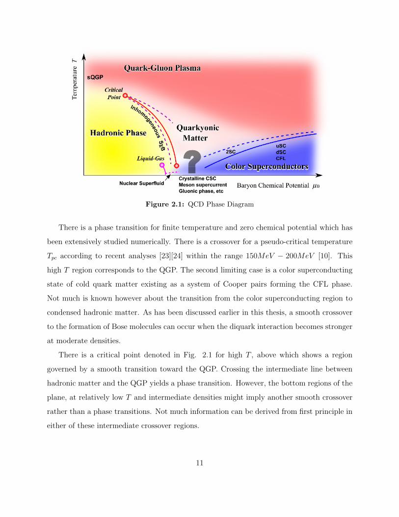
Figure 2.1 is a schematic representation in the temperature-density plane of known phases
of QCD [10].
At baryonic chemical potential around µNM = 924MeV and T = 0 nuclear matter starts
to form, and in this region of the graph the familiar critical point of a phase transition
between the familiar hadronic matter, mesons and baryons, makes up the low temperature
and low density corner of the graph. In the outer regions of the temperature density plane,
our current understanding only allows us to make strong statements on limiting cases, such
as high T and relatively small density or, as in this thesis, asympotically high density and
low vanishing T . The first of these cases leads to a region of deconfinement where individual
quarks are too energetic to remain in bound states from the strong nuclear interaction which
is the state of matter thought to have existed in the early universe and known as the quark-
gluon plasma (QGP).
10
Page 19
Figure 2.1: QCD Phase Diagram
There is a phase transition for finite temperature and zero chemical potential which has
been extensively studied numerically. There is a crossover for a pseudo-critical temperature
Tpc according to recent analyses [23][24] within the range 150MeV − 200MeV [10]. This
high T region corresponds to the QGP. The second limiting case is a color superconducting
state of cold quark matter existing as a system of Cooper pairs forming the CFL phase.
Not much is known however about the transition from the color superconducting region to
condensed hadronic matter. As has been discussed earlier in this thesis, a smooth crossover
to the formation of Bose molecules can occur when the diquark interaction becomes stronger
at moderate densities.
There is a critical point denoted in Fig. 2.1 for high T , above which shows a region
governed by a smooth transition toward the QGP. Crossing the intermediate line between
hadronic matter and the QGP yields a phase transition. However, the bottom regions of the
plane, at relatively low T and intermediate densities might imply another smooth crossover
rather than a phase transitions. Not much information can be derived from first principle in
either of these intermediate crossover regions.
11
Page 20
We will want to investigate how equations of state behave throughout the BCS-BEC
crossover in order to understand how the dynamical properties of our systems will change.
2.5 BCS-BEC crossover
The attraction binding ultracold fermionic pairs in atomic physics can be tuned via Feshbach
resonance where an applied magnetic field is used to adjust the interaction. Crossovers
between BCS and BEC dynamics have already been observed [2]. In tuning the interaction
the coherence length of the Cooper pairs is altered. In the BCS regime the coherence length
is much larger than the interparticle spacing. However, for BEC dynamics to occur at larger
coupling strength that can reducing the interparticle distance enough to form Bose molecules,
the fermionic degrees of freedom have to be removed.
As for dense quark matter in particular, strong theoretical developments now exist indi-
cating that by tuning the interaction strength between the quarks forming the Cooper pairs
we can drive the system between domains of BCS and BEC dynamics [5], and several models
have already been proposed [17]-[21]. This section serves to introduce a general layout for
the methods and definitions used in defining the crossover parameter in the models presented
later in Chapters 3 and 4
The Pauli exclusion principle prevents half-integer spin particles from occupying the same
quantum states, however, bosons having integral spin means they are not subject to this
restriction. Therefore, a uniformly distributed system of bosons may act as free particles
giving rise to color superconductivity. Color superconductivity can also be realized for a
system of fermions according to BCS theory by the formation of Cooper pairs composed
of different color quarks [9] with opposite momentum near the Fermi-surface. Now, let us
discuss in a simple way how the BCS-BEC crossover takes place in a relativistic system [3].
The dispersion of the quasiparticles in a superconductor is given by
εk =√
(εk0 − µ)2 + ∆2 (2.15)
12
Page 21
where for relativistic energies
εk0 =√m2 + k2. (2.16)
From Eq. (2.15) we find that the energy minimum in k has two values, one at k =√µ2 −m2
and another at k = 0. It can be seen that the minimum at k =√µ2 −m2 results in a lower
energy than that at k = 0, and is thus the true minimum provided that µ ≥ m. However,
if µ ≤ m then the first minima disappears due to not returning a real value, leaving k = 0
as the minimum. With the first minima we have an energy gap ∆ as is the case for a BCS
state, while the second minima leaves an energy gap of√
(m− µ)2 + ∆2 which corresponds
to a BEC state of matter. Because the two minima, as well as the energy gaps for both BCS
and BEC, are equal for µ = m this suggests a smooth crossover between the two regions
rather than an abrupt phase transition.
2.6 Newton’s Method
In chapters 3 and 4 it will become necessary to solve systems of integral equations for the
energy gap (∆) and chemical potential (µ) which require us to resort to numerical techniques.
One such technique is called Newton’s method, which we will use in this section to derive a
solution that may be applied to the specific cases that will arise later.
Newton’s method is a technique for finding approximately the roots for equations of the
form f(x) = 0. For functions of a single variable Newton’s method is summarized in the
following iterative equation
xn+1 = xn −f(xn)
f ′(xn)(2.17)
where xn+1 is a better approximation to the true solution than was xn. x0 is often chosen
as a best guess, or in order to ensure convergence of the series. For systems of equations
involving more than one variable of the form fi(x) = 0 where x is a column vector, and each
13
Page 22
of the fi(x) is an element in the column vector F, then Eq (2.17) becomes
J y = F (2.18)
in which J is the Jacobian matrix having elements
Jij =∂Fi∂xj
(2.19)
and y is the column vector y = xn+1−xn representing the correction to xn for each iteration.
In the special case in which we have a system of two equations with two variables, meaning
F and y are 2 component vectors and the Jacobian, J , is a 2 × 2 matrix, then a general
solution can be found for y1 and y2, as
y1 =(J22J12F1 − F2
)J12
J12J21−J11J22
y2 = −F1+J11y1J12 .
(2.20)
The above equations is our general solution which will be used in Chapters 3 and 4 to solve
the systems of integral equations. The integrals themselves will also be solved numerically
using the trapezoidal rule. The final values, y, are then added to xn and the process is
repeated until
F ≤ ε, (2.21)
where ε is an acceptably low error.
14
Page 23
Chapter 3
Equations of State in a Relativistic
Boson-Fermion System
This Chapter studies the BCS-BEC crossover for color superconducting regimes by using a
relativistic model that possesses both bosonic and fermionic degrees of freedom [20]. There-
fore, it is expected that the density of fermions should vanish when entering the BEC region
and vice versa. This is in contrast to the purely fermionic model presented in Chapter 4 in
which there is only fermionic degrees of freedom.
3.1 Composite-Boson-Fermion model
The bosons are expected to form at lower densities when asymptotic freedom is broken and
the quarks are no longer able to exist as free particles. In that case, quarks bind together
into diquark molecules. In this model we treat independently the boson molecules that exist
in the strong coupling regime, and the composite diquarks which are expected to form as
Cooper pairs in the weak coupling regime. They will appear as different fields contributing
to the Lagrangian. We will refer to the system as either being BCS or BEC based on which
dispersion relation (Eq (3.8) and graphed in Fig. 3.2) describes the quasiparticles in each
region in question. The Lagrangian is composed of a bosonic (L0) and fermionic (LF ) term
with a Yukawa interaction between the two (LI):
L = Lf + Lb + LI (3.1)
15
Page 24
where
Lf = ψ (iγµ∂µ + γ0µ−m)ψ
Lb = | (∂t − iµb)ϕ|2 − |∇ϕ|2 −mb|ϕ|2
LI = g(ϕψCiγ5ψ + ϕ∗ψiγ5ψC
) (3.2)
Here, C = iγ2γ0 is the charge conjugate matrix, and ψC = CψT and ψC = ψTC are the
charge conjugate spinors. We also impose the restriction that µb = 2µ to ensure equilibrium
between fermion and boson conversions. Then, in the mean-field approximation in which
φ = 〈ϕ0〉 is the vaccuum expectation value of the boson field, we find in the Nambu-Gorkov
space with spinors
Ψ =
ψ
ψC
, Ψ =(ψ, ψC
)(3.3)
the Lagrangian density
L =1
2ΨS−1Ψ + (µ2
b −m2b)|φ|2 + |(∂t − iµb)φ|2 − |∆φ|2 −m2
b |φ|2 (3.4)
with inverse fermion propagator given by
S−1(P ) =
Pµγµ + µγ0 −m 2igγ5φ
∗
2igγ5φ Pµγµ − µγ0 −m
. (3.5)
As it is characteristic of the mean-field approximation we neglect the interaction between
the fermions and the fluctuating boson fields.
The thermodyanmic potential density at finite temperature T is then computed beginning
with the partition function from Eq. (2.3). In our case with fermionic and bosonic fields this
is
Z =
∫[dψ][dψ][dφ][dφ∗]e
∫ 1/T0 dτd3xL. (3.6)
16
Page 25
Plugging the above into Eq. (2.4) yields
Ω = −∑
e=±∫
d3k(2π)3
[εek + 2T ln
[1 + exp
(− εek
T
)]]+
(m2b−µ
2b)∆2
4g2
+12
∑e=±
∫d3k
(2π)3
[ωek + 2T ln
[1− exp
(−ωe
k
T
)]],
. (3.7)
where the terms involving the quasiparticle energy are denoted by
εek =
√(εk0 − eµ)2 + ∆2 εk0 =
√k2 +m2 ωek =
√k2 +m2
b − eµb, (3.8)
with e = ±1 corresponding to fermions and antifermions for plus and minus respectively, and
∆ = 2gφ. We are particularly interested in the zero-temperature limit of the thermodynamic
potential
Ω0 = −∑e=±
∫d3k
(2π)3 εek +
(m2b − µ2
b) ∆2
4g2+
1
2
∑e=±
∫d3k
(2π)3ωek. (3.9)
In this model we renormalize the boson mass rather than the coupling, by the condition
m2b,r = 4g2 ∂Ω
∂∆2
∣∣∣∣∆=µ=T=0
= m2b − 4g2
∫d3k
(2π)3
1
εk0. (3.10)
The crossover parameter that will be used is defined as follows
x = −m2b,r − µ2
b
4g2, (3.11)
Hence, from Eqs. (3.10) and (3.11) the dynamical boson mass is given in terms of the
crossover parameter as
m2b − µ2
b = 4g2
(∫d3k
(2π)3
1
εk0− x)
= 4g2(x0 − x). (3.12)
Then, for small enough fermion masses (m Λ, where Λ is the momentum cutoff), we have
x0 ≈Λ2
4π2. (3.13)
17
Page 26
3.2 Gap Equation at Fixed Fermion Density
Now, to find solutions for µ and ∆ we can make use of two additional conditions. First,
because each momentum state in the Fermi sphere can only be occupied by two fermions of
opposite spin, there exists a relation between the particle density in momentum space and
the Fermi momentum. The second condition is that the energy gap produced by the Cooper
pairs should minimize the thermodynamic potential. These two conditions are summarized
in the following equations respectively
∂Ω0
∂µ= − P
3F
3π2(3.14)
∂Ω0
∂∆= 0. (3.15)
Substituting Eq. (3.9) into the above yields
(P 3F
3π2
)=
1
2π2
∫ 1
0
k2dk
[ξ+k
ε+k− ξ−kε−k
]+
2
g2µ∆2 (3.16)
− x
x0
= 2
∫ 1
0
k2dk
[1
ε+k+
1
ε−k− 2
εk0
](3.17)
with
ξek = εk − eµ. (3.18)
3.3 Numerical Solutions
To solve the set of Eqs. (3.16)-(3.17) we resort to numerical methods with the following
parameters fixed: the upper limit of momentum Λ = 602.3MeV, PF = 0.3Λ, m = 0.4Λ, and
g = 4/Λ2. The procedure now follows the methods described in section 2.6 to adapt them
18
Page 27
0
0.1
0.2
0.3
0.4
0.5
0.6
0.7
-0.4 -0.3 -0.2 -0.1 0 0.1 0.2
x/x0
µ~
∆~m
Figure 3.1: µ and ∆ vs. the crossover parameter x/x0, where µ = µ/Λ and ∆ = ∆/Λ
0
0.2
0.4
0.6
0.8
1
1.2
1.4
1.6
0 0.1 0.2 0.3 0.4 0.5 0.6 0.7 0.8 0.9 1
ε~k
+
k~
x/x0 = -0.45
x/x0 = 0.005
x/x0 = 0.4
Figure 3.2: Quasiparticle dispersion curves of Eq. (3.8) for various values of x/x0
19
Page 28
0
0.1
0.2
0.3
0.4
0.5
0.6
0.7
0.8
0.9
1
-0.5 -0.4 -0.3 -0.2 -0.1 0 0.1 0.2 0.3 0.4 0.5
x/x0
ρ0ρF
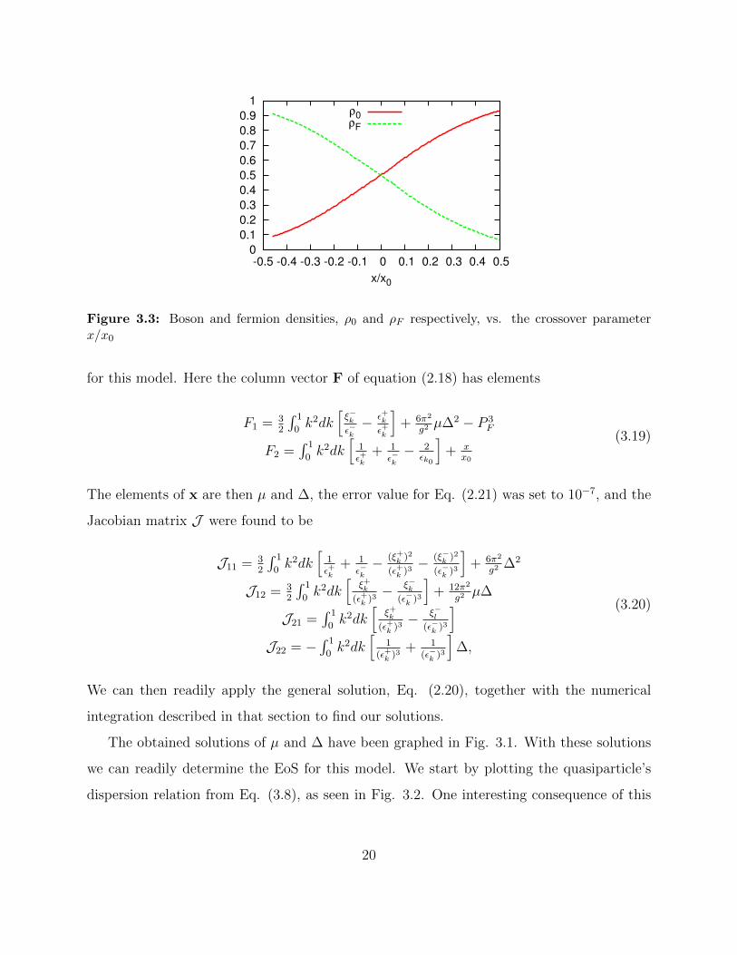
Figure 3.3: Boson and fermion densities, ρ0 and ρF respectively, vs. the crossover parameterx/x0
for this model. Here the column vector F of equation (2.18) has elements
F1 = 32
∫ 1
0k2dk
[ξ−kε−k− ε+k
ε+k
]+ 6π2
g2µ∆2 − P 3
F
F2 =∫ 1
0k2dk
[1ε+k
+ 1ε−k− 2
εk0
]+ x
x0
(3.19)
The elements of x are then µ and ∆, the error value for Eq. (2.21) was set to 10−7, and the
Jacobian matrix J were found to be
J11 = 32
∫ 1
0k2dk
[1ε+k
+ 1ε−k− (ξ+k )2
(ε+k )3− (ξ−k )2
(ε−k )3
]+ 6π2
g2∆2
J12 = 32
∫ 1
0k2dk
[ξ+k
(ε+k )3− ξ−k
(ε−k )3
]+ 12π2
g2µ∆
J21 =∫ 1
0k2dk
[ξ+k
(ε+k )3− ξ−l
(ε−k )3
]J22 = −
∫ 1
0k2dk
[1
(ε+k )3+ 1
(ε−k )3
]∆,
(3.20)
We can then readily apply the general solution, Eq. (2.20), together with the numerical
integration described in that section to find our solutions.
The obtained solutions of µ and ∆ have been graphed in Fig. 3.1. With these solutions
we can readily determine the EoS for this model. We start by plotting the quasiparticle’s
dispersion relation from Eq. (3.8), as seen in Fig. 3.2. One interesting consequence of this
20
Page 29
-0.1
-0.08
-0.06
-0.04
-0.02
0
0.02
0.04
0.06
0.08
0.1
-0.4 -0.2 0 0.2 0.4 0.6 0.8
x/x0
p
ε
Figure 3.4: Pressure and energy density p = p/Λ4 ε = ε/Λ4 vs. the crossover parameter x/x0.
graph is that according to the explanation in section 2.4, we observe a bosonic like curve
for x/x0 larger than the critical value where the system crosses over to the BEC regime,
as indicated by the chemical potential becoming smaller than th mass in Fig. 3.1. This
means that even though we model the system as separate boson and fermion contributions
the quasiparticles behave as bosons in the strong coupling regime.
Now we investigate the system EoS using the solutions for chemical potential and gap
just found. The energy density and pressure are given respectively by ε = Ω0 + µn and
p = −Ω0. To guarantee that the system pressure and energy become zero in vacuum (i.e.
when µ = ∆ = 0) we introduce
ε = Ω0 + µn− Ωvac0
p = −Ω0 + Ωvac0
Ωvac0 = Ω0(µ = ∆ = 0).
(3.21)
Next we analyze with the fractional densities of fermions (ρF = nF/n) and bosons (ρ0 = n0/n),
such that n = n0 + nF , where
nF = −∂Ω
∂µ, n0 =
2µ∆2
g2, n =
P 3F
3π2. (3.22)
21
Page 30
As you can see in Fig. 3.3 the system is primarily composed of fermions with a low boson
density when x/x0 < 0, highlighting the BCS portion of the x/x0 domain, while in the right
half of the graph, for x/x0 > 0, there consists of a high boson and low fermion density
corresponding to the BEC region.
The numerical solutions previously found are now used to examine the EoS (i.e. the pres-
sure and energy), displayed in Fig. 3.4. The dominant term in Ω0 is the bosonic contribution
throughout both BCS and BEC regimes, however, once the vacuum term Ωvac is subtracted
the bosonic contribution essentially disappears. The sign in the middle term of Eq. (3.9)
is determined by m2b − µ2
b which changes roughly around the crossover when µ = m. So
the middle term contributes a positive pressure to the BCS region, yet turns negative just
before the crossover to the BEC region. As for the fermionic contribution to the pressure, it
is positive throughout both regions. Therefore, it is this middle, fermion-boson interaction,
term which makes the pressure unstable in the far BEC region.
Further investigation shows that the same results as above may also be obtained for
various values of m and mb. The values used in this thesis were chosen to agree with the
originally proposed model [20], as well as to highlight the pressure instability that may
occur in the far BEC regime. These two considerations required careful balancing due to
limitations of the numerical methods used. Additionally, the presence of a positive pressure
in the BCS region with a decreasing pressure, together with the instability, toward the BEC
region agree with expectations, because of the lack of Pauli exclusion principle once the
quasiparticles become bosonic.
22
Page 31
Chapter 4
Fermionic Model for a Relativistic
Superfluid
This model describes a system with only fermionic degrees of freedom and multi-fermion
interactions. The attractive channel between quarks allows the formation of diquarks in
the strong coupling regime. The diquarks play the role of the bosonic field used in chapter
3. Additionally there exists a diquark-diquark repulsive channel [16] parameterized by the
coupling constant λ.
4.1 Purely-Fermionic model
For this investigation we consider a simple relativistic model of fermions with multi-fermion
interactions represented in the Lagrangian density
L = ψ (iγµ∂µ −m)ψ + LI + L′I (4.1)
where
LI =g
4
(ψiγ5Cψ
T) (ψTCiγ5ψ
)
L′I = −λ[(ψiγ5Cψ
T) (ψTCiγ5ψ
)]2,
m is the fermion mass, µ the chemical potential, g the fermion-fermion coupling constant, λ
the diquark-diquark repulsive constant, and C = iγ0γ2 the charge conjugation matrix.
23
Page 32
0.37
0.38
0.39
0.4
0.41
0.42
0.43
0.44
0.45
18 20 22 24 26 28 30 32 34 36 38
µ
g~
λ=0
λ=0.1
λ=1
λ=10
m
Figure 4.1: Chemical potential µ versus coupling constant g = gΛ2 plotted for different values ofλ.
With LI above simulating the quark-quark attractive interaction and the second, primed,
term L′I with λ > 0 corresponding to a diquark-diquark repulsive interaction. From this La-
grangian density (4.1) and the procedure outlined in Section 2.4 the thermodynamic potential
can be calculated [20], which at T = 0 is
Ω0 = −∑e=±1
∫Λ
d3k
(2π)3εek +
∆2
g+ λ∆4 (4.2)
With the energy spectrum, εek, given by
εek =
√(εk0 − eµ)2 + ∆2 (4.3)
εk0 =√k2 +m2
and e = ±1, which corresponds to particles for positive, and antiparticles for negative.
24
Page 33
0
0.01
0.02
0.03
0.04
0.05
0.06
20 22 24 26 28 30 32 34 36
∆
g~
λ=0
λ=0.1
λ=1
λ=10
Figure 4.2: Energy gap ∆ versus coupling constant g = gΛ2 plotted for different values of λ.
4.2 Numerical solutions
Similar to Chapter 3, the goal is now to find solutions for µ and ∆ from the thermodynamic
potential, Eq. (4.2). This is done with the particle density equation fixed by the Fermi
momentum
P 3F = 3π2∂Ω0
∂µ= −3
2
∫Λ
dkk2
[ξ+k
ε+k− ξ−kε−k
](4.4)
and the gap equation ∂Ω0/∂∆ = 0 that can be written as
1 =g
4π2
∫Λ
dkk2
[1
ε+k+
1
ε−k
]− 2λg∆2 (4.5)
where
ξek = εk − eµ (4.6)
Once more employing the general solution of Eq. (2.20) we have
F1 = 32
∫ 1
0dkk2
[ξ−kε−k− ξ+k
ε−k
]−(PF
Λ
)3
F2 = g4π2
∫ 1
0dkk2
[1ε+k
+ 1ε−k
]− 2λg∆2 − 1
(4.7)
25
Page 34
and the elements of the Jacobian
J11 = 32
∫ 1
0dkk2
[1ε+k
+ 1ε−k− (ξ+k )2
(ε+k )3− (ξ−k )2
(ε−k )3
]J12 = 3
2
∫ 1
0dkk2
[ξ+k
(ε+k )3− ξ−k
(ε−k )3
]∆
J21 = g4π2
∫ 1
0dkk2
[ξ+k
(ε+k )3− ξ−k
(ε−k )3
]J22 = − g
4π2
∫ 1
0dkk2
[1
(ε+k )3+ 1
(ε−k )3
]∆− 4λg∆
(4.8)
In solving this system of integral equations we fix the other parameters to represent a
relativistic quark gas [19], Λ = 602.3MeV the cutoff in the momentum integral, m/Λ = 0.4
the fermionic mass, and PF/Λ = 0.3 the Fermi momentum, and the results are graphed in
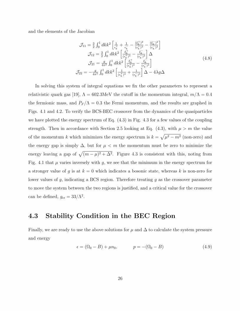
Figs. 4.1 and 4.2. To verify the BCS-BEC crossover from the dynamics of the quasiparticles
we have plotted the energy spectrum of Eq. (4.3) in Fig. 4.3 for a few values of the coupling
strength. Then in accordance with Section 2.5 looking at Eq. (4.3), with µ > m the value
of the momentum k which minimizes the energy spectrum is k =√µ2 −m2 (non-zero) and
the energy gap is simply ∆, but for µ < m the momentum must be zero to minimize the
energy leaving a gap of√
(m− µ)2 + ∆2. Figure 4.3 is consistent with this, noting from
Fig. 4.1 that µ varies inversely with g, we see that the minimum in the energy spectrum for
a stronger value of g is at k = 0 which indicates a bosonic state, whereas k is non-zero for
lower values of g, indicating a BCS region. Therefore treating g as the crossover parameter
to move the system between the two regions is justified, and a critical value for the crossover
can be defined, gcr = 33/Λ2.
4.3 Stability Condition in the BEC Region
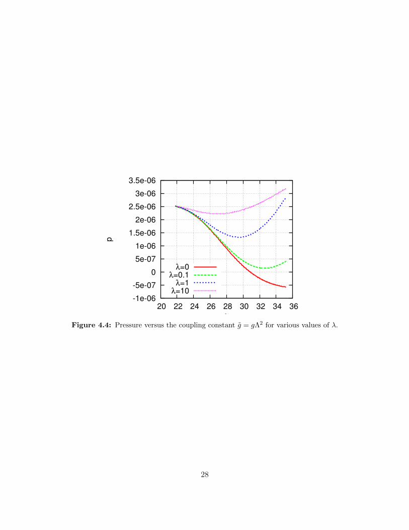
Finally, we are ready to use the above solutions for µ and ∆ to calculate the system pressure
and energy
ε = (Ω0 −B) + µn0, p = −(Ω0 −B) (4.9)
26
Page 35
0
50
100
150
200
250
300
350
400
450
0 100 200 300 400 500 600 700
ε k+
k
g~ =20g~ =28g~ =36
Figure 4.3: ε+k vs k plotted for different values of the coupling strength g = gΛ2.
where in this model the vacuum is treated as a constant, B, whose value is determined
by setting the pressure to zero. Pressure is plotted in Fig. 4.4, and as can be seen the
λ = 0 solution becomes negative before the critical value (gcr = 33/Λ2), therefore this
solution doesn’t allow for BEC dynamics at all due to unstable pressure. Although a similar
comparison shows that the other solutions for larger values of λ do permit BEC dynamics
with positive pressure in this particular model.
27
Page 36
-1e-06
-5e-07
0
5e-07
1e-06
1.5e-06
2e-06
2.5e-06
3e-06
3.5e-06
20 22 24 26 28 30 32 34 36
p
g~
λ=0
λ=0.1
λ=1
λ=10
Figure 4.4: Pressure versus the coupling constant g = gΛ2 for various values of λ.
28
Page 37
Chapter 5
Final Remarks
We study the BCS-BEC crossover for two relativistic systems. One formed by fermions and
bosons interacting through a Yukawa potential. The other, only having fermionic degrees
of freedom under multi-fermion interactions that account for a fermion-fermion attractive
channel and a difermion-difermion repulsion. The main goal of this investigations was to
analyze the evolution of the system EoS throughout the crossover.
We have found for the boson-fermion model that the system pressure is positive through-
out the entire BCS domain. In the BEC domain the pressure decreases to negative values
indicating an instability. Before this instability occurs in the BEC region the pressure is
positive and the graph actually displays an interesting downward concavity in the curve. In
separating out the individual contributions to the pressure from each term it is observed
that this inflection point is caused by a shift in dominance from the fermionic term given
by an integral over the fermionic dispersion to the term contributed by the fermion-boson
interaction (middle term) in Eq. (3.9).
In our simple fermion model the pressure displayed the expected decreasing behavior
when the system crosses over from the BCS to the BEC region. In the case in which the
diquark-diquark repulsion term was added to the thermodynamic potential it seems possible
that the system could remain stable for all values of the coupling, g, in the BEC region [25].
Therefore, in this simple fermionic model we observe a stable BCS region which crosses over
into stable BEC dynamics once the diquark-diquark repulsion is strong enough. However, our
investigation was limited up to the λ∆4 tree-level contribution. A more detailed investigation
would introduce additional terms to the quasiparticle spectrum.
It appears the the two models are qualitatively in agreement as to the stability of the
29
Page 38
star, with both stable BCS and BEC dynamics and an eventual instability arising deeper
into the BEC region. One difference between the results that stands out is the existence of
a maximum in the pressure in the middle of the BEC region for our fermion-boson model,
wheras no such maximum exists in the simple fermion model. In the limit of low chemical
potential, which is the case near this maximum, it can be seen that the equations describing
the pressure in the two models becomes very similar. Yet, this difference between the two
models still occurs due to the fact that the diquark-diquark repulsion in the simple fermion
model enters into the calculations of µ and ∆ as seen in Eq. (4.8).
As a physical interpretation of the instabilities described in this paper, note that the
instabilities are thought to merely indicate where the model no longer describes a diquark
BEC state, rather than an actual instability in the star. The graphs show that the instabil-
ities would exist at lower densities within the neutron star which could possibly mean that
the density is low enough for hadronization to take place.
30
Page 39
References
[1] D. J. Gross and F. Wilczek, Phys. Rev. Lett. 30, 1343 (1973).
[2] K. I. Wysokinski, arXiv:1111.5318 [physics.hist-ph].
[3] G. -f. Sun, L. He and P. Zhuang, Phys. Rev. D 75, 096004 (2007) [hep-ph/0703159].
[4] E. J. Ferrer, V. de la Incera, J. P. Keith, I. Portillo and P. L. Springsteen, Phys. Rev.
C 82, 065802 (2010) [arXiv:1009.3521 [hep-ph]].
[5] M. Randeria and E. Taylor, Physics 5, 209 (2014) [arXiv:1306.5785 [cond-mat.quant-
gas]].
[6] I. A. Shovkovy, Found. Phys. 35, 1309 (2005) [nucl-th/0410091].
[7] L. N. Cooper, Phys. Rev. 104, 1189 (1956).
[8] C. Kittel and H. Kroemer, W. H. Freeman and Company, 1980, New York, NY.
[9] M. G. Alford, A. Schmitt, K. Rajagopal and T. Schfer, Rev. Mod. Phys. 80, 1455 (2008)
[arXiv:0709.4635 [hep-ph]].
[10] K. Fukushima and T. Hatsuda, Rept. Prog. Phys. 74, 014001 (2011) [arXiv:1005.4814
[hep-ph]].
[11] M. G. Alford, K. Rajagopal and F. Wilczek, Nucl. Phys. B 537, 443 (1999) [hep-
ph/9804403].
[12] Z. G. Wang, S. L. Wan and W. M. Yang, hep-ph/0508302.
[13] M. Huang, P. -f. Zhuang and W. -q. Chao, Chin. Phys. Lett. 19, 644 (2002) [hep-
ph/0110046].
¡UNUSED¿
31
Page 40
[14] M. Huang, P. -f. Zhuang and W. -q. Chao, Phys. Rev. D 65, 076012 (2002) [hep-
ph/0112124].
[15] M. Huang, Int. J. Mod. Phys. E 14, 675 (2005) [hep-ph/0409167].
[16] F. Wilczek, In *Shifman, M. (ed.) et al.: From fields to strings, vol. 1* 77-93 [hep-
ph/0409168].
[17] Y. Nishida and H. Abuki, Phys. Rev. D 72, 096004 (2005) [hep-ph/0504083].
[18] L. He and P. Zhuang, Phys. Rev. D 75, 096003 (2007) [hep-ph/0703042].
[19] E. J. Ferrer and J. P. Keith, Phys. Rev. C 86, 035205 (2012) [arXiv:1201.2203 [nucl-th]].
[20] J. Deng, A. Schmitt and Q. Wang, Phys. Rev. D 76, 034013 (2007) [nucl-th/0611097].
[21] A. H. Rezaeian and H. J. Pirner, Nucl. Phys. A 779, 197 (2006) [nucl-th/0606043]. L. He
and P. Zhuang, Phys. Rev. D 76, 056003 (2007) [arXiv:0705.1634 [hep-ph]]. G. -f. Sun,
L. He and P. Zhuang, Phys. Rev. D 75, 096004 (2007) [hep-ph/0703159]. H. Abuki,
Nucl. Phys. A 791, 117 (2007) [hep-ph/0605081]. M. Kitazawa, D. H. Rischke and
I. A. Shovkovy, Phys. Lett. B 663, 228 (2008) [arXiv:0709.2235 [hep-ph]]. H. Abuki
and T. Brauner, Phys. Rev. D 78, 125010 (2008) [arXiv:0810.0400 [hep-ph]]. J. Deng,
J. -c. Wang and Q. Wang, Phys. Rev. D 78, 034014 (2008) [arXiv:0803.4360 [hep-ph]].
D. Blaschke and D. Zablocki, Phys. Part. Nucl. 39, 1010 (2008) [arXiv:0812.0589 [hep-
ph]]. T. Brauner, Phys. Rev. D 77, 096006 (2008) [arXiv:0803.2422 [hep-ph]]. J. O. An-
dersen, Nucl. Phys. A 820, 171C (2009) [arXiv:0809.2892 [hep-ph]]. H. Guo, C. -C. Chien
and Y. He, Nucl. Phys. A 823, 83 (2009) [arXiv:0812.1782 [hep-ph]]. B. Chatterjee,
H. Mishra and A. Mishra, Phys. Rev. D 79, 014003 (2009) [arXiv:0804.1051 [hep-ph]].
T. Hatsuda, M. Tachibana, N. Yamamoto and G. Baym, Phys. Rev. Lett. 97, 122001
(2006) [hep-ph/0605018]. N. Yamamoto, M. Tachibana, T. Hatsuda and G. Baym,
Phys. Rev. D 76, 074001 (2007) [arXiv:0704.2654 [hep-ph]]. T. Hatsuda, M. Tachibana
32
Page 41
and N. Yamamoto, Phys. Rev. D 78, 011501 (2008) [arXiv:0802.4143 [hep-ph]]. N. Ya-
mamoto and T. Kanazawa, Phys. Rev. Lett. 103, 032001 (2009) [arXiv:0902.4533 [hep-
ph]]. H. Basler and M. Buballa, Phys. Rev. D 82, 094004 (2010) [arXiv:1007.5198 [hep-
ph]]. H. Abuki, G. Baym, T. Hatsuda and N. Yamamoto, Phys. Rev. D 81, 125010
(2010) [arXiv:1003.0408 [hep-ph]]. J. -c. Wang, Q. Wang and D. H. Rischke, Phys. Lett.
B 704, 347 (2011) [arXiv:1008.4029 [nucl-th]]. J. -c. Wang, V. de la Incera, E. J. Ferrer
and Q. Wang, Phys. Rev. D 84, 065014 (2011) [arXiv:1012.3204 [nucl-th]].
[22] J. Ranninger, arXiv:1207.6911 [cond-mat.supr-con].
[23] Y. Aoki, G. Endrodi, Z. Fodor, S. D. Katz and K. K. Szabo, Nature 443, 675 (2006)
[hep-lat/0611014].
[24] C. DeTar and U. M. Heller, Eur. Phys. J. A 41, 405 (2009) [arXiv:0905.2949 [hep-lat]].
[25] E. J. Ferrer, V. de la Incera, J. P. Keith and I. Portillo, arXiv:1405.7422 [hep-ph].
[26] R. Casalbuoni, R. Gatto, M. Mannarelli, G. Nardulli and M. Ruggieri, Phys. Lett. B
605, 362 (2005) [Erratum-ibid. B 615, 297 (2005)] [hep-ph/0410401]. M. Alford and
Q. -h. Wang, J. Phys. G 31, 719 (2005) [hep-ph/0501078]. K. Fukushima, Phys. Rev.
D 72, 074002 (2005) [hep-ph/0506080].
[27] P. F. Bedaque and T. Schfer, Nucl. Phys. A 697, 802 (2002) [hep-ph/0105150]. A. Kry-
jevski and T. Schfer, Phys. Lett. B 606, 52 (2005) [hep-ph/0407329]. A. Gerhold and
T. Schfer, Phys. Rev. D 73, 125022 (2006) [hep-ph/0603257].
[28] M. G. Alford, J. A. Bowers and K. Rajagopal, Phys. Rev. D 63, 074016 (2001)
[hep-ph/0008208]. I. Giannakis and H. -C. Ren, Phys. Lett. B 611, 137 (2005) [hep-
ph/0412015]. R. Casalbuoni, R. Gatto, N. Ippolito, G. Nardulli and M. Ruggieri, Phys.
Lett. B 627, 89 (2005) [Erratum-ibid. B 634, 565 (2006)] [hep-ph/0507247]. M. Cim-
inale, G. Nardulli, M. Ruggieri and R. Gatto, Phys. Lett. B 636, 317 (2006) [hep-
33
Page 42
ph/0602180]. K. Rajagopal and R. Sharma, Phys. Rev. D 74, 094019 (2006) [hep-
ph/0605316].
[29] E. J. Ferrer and V. de la Incera, Phys. Rev. Lett. 97, 122301 (2006) [hep-ph/0604136].
34
Page 43
Curriculum Vitae
Jason Keith received his Bachelor of Science degree in Physics from the University of Texas
at El Paso in 2012. During this degree he was awarded for research excellence by the College
Office of Undergraduate Initiatives (COURI) and the Department of Physics, inducted into
the Sigma Pi Sigma physics honor society, and engaged in research with Dr. Ferrer and the
high-energy theory group at UTEP which lead to a publication (Phys.Rev.C82:065802,2010).
As an undergraduate he also had many opportunities to go to conferences and present re-
search, spent one summer at Virginia Tech for an REU, and worked on campus as a TA.
Continuing with his education he began working toward an M.S. degree in physics which
will be completed in Spring of 2014 pending the approval of this Thesis.
35