PHYSICAL REVIEW A VOLUME 39, NUMBER 4 FEBRUARY 15, 1989 Equilibrium and nonequilibrium Lyapunov spectra for dense fluids and solids Harald A. Posch Institute for Experimental Physics, University of Vienna, Boltzmanngasse 5, Vienna A-1090, Austria William G. Hoover Department ofApplied Science, University of California at Davis-Livermore and Lawrence Livermore National Laboratory, Box 808, Livermore, California 94550 (Received 16 August 1988) The Lyapunov exponents describe the time-averaged rates of expansion and contraction of a La- grangian hypersphere made up of comoving phase-space points. The principal axes of such a hyper- sphere grow, or shrink, exponentially fast with time. The corresponding set of phase-space growth and decay rates is called the "Lyapunov spectrum." Lyapunov spectra are determined here for a variety of two- and three-dimensional fluids and solids, both at equilibrium and in nonequilibrium steady states. The nonequilibrium states are all boundary-driven shear flows, in which a single boundary degree of freedom is maintained at a constant temperature, using a Nose-Hoover ther- mostat. Even far-from-equilibrium Lyapunov spectra deviate logarithmically from equilibrium ones. Our nonequilibrium spectra, corresponding to planar-Couette-flow Reynolds numbers rang- ing from 13 to 84, resemble some recent approximate model calculations based on Navier-Stokes hydrodynamics. We calculate the Kaplan-Yorke fractal dimensionality for the nonequilibrium phase-space flows associated with our strange attractors. The far-from-equilibrium dimensionality may exceed the number of additional phase-space dimensions required to describe the time depen- dence of the shear-flow boundary. I. INTRODUCTION Over 100 years ago Boltzmann emphasized the prob- lem of reconciling the irreversible macroscopic behavior of atomistic systems with the time-reversal invariance of the underlying equations of motion. I But Boltzmann's H-theorem explanation was criticized because the irrever- sibility inherent in his equation was based on statistical arguments rather than mechanical principles. Under- standing the connection between macroscopic irreversi- bility and microscopic reversibility has remained a con- stant challenge. Only recently has a more complete pic- 5 ture been developed. 2 - The key concepts underlying this understanding are fractal strange attractors and re- pellors, in phase space, and their relation to the novel nonequilibrium molecular-dynamics simulation tech- niques made possible by modern supercomputers. 6 Through computer simulation it has finally become possi- ble to extend Boltzmann's H-theorem explanation of ir- reversibility. This new understanding of irreversible behavior is based on the phase-space description of nonequilibrium systems. The time development of systems, either at or away from equilibrium, is most concisely described in terms of the phase trajectory in that space. The mathematical stability of the motion, and the quantita- tive characterization of the irreversibility described by the second law of thermodynamics, require that the motion of a set of contiguous phase points be studied. - This set can be visualized as a co moving hypersphere, centered on an ordinary "reference trajectory." The de- formation of such a hypersphere then needs to be de- scribed. As has been emphasized repeatedly7 the motion in cases corresponding to a statistical thermodynamic or hydrodynamic description is "Lyapunov unstable." This means that neighboring initial points separate from one another exponentially fast in time. At the same time these "unstable" nonequilibrium motions are actually stable in the sense that they explore only a restricted por- tion of phase space, a "strange attract or" with a dimen- sionality less than that of the equilibrium phase space. Within the limited subspace occupied by the attractor, the trajector comes close to a fractal set of points in the same sense that the Peano curve, shown in Fig. 1, comes close to the points in a two-dimensional unit square. But the mechanism for the covering of the attractor is different from the smaller-and-smaller-scale turnings of a Peano curve. Smale emphasized that phase-space mixing occurs through a "Smale horseshoe" deformation that simultaneously incorporates the expanding and contract- ing motions characteristic of chaotic time-reversible dynamical systems. 8 ,9 These phase-space flows can be partially characterized in terms of their spectrum of Lyapunov characteristic ex- ponents. The results obtained so far for many-particle systems both in equilibrium and nonequilibrium steady states can be summarized as follows. (1) Equilibrium reversible Hamiltonian systems have Lyapunov spectra made up of pairs ( that sum to zero. This symmetric distribution, with zero sum, corre- sponds to the conservation of phase-space volume de- tailed by Liouville's theorem. As may be verified from 39 2175 1989 The American Physical Society
Transcript
PHYSICAL REVIEW A VOLUME 39 NUMBER 4 FEBRUARY 15 1989
Equilibrium and nonequilibrium Lyapunov spectra for dense fluids and solids
Harald A Posch Institute for Experimental Physics University of Vienna Boltzmanngasse 5 Vienna A-1090 Austria
William G Hoover Department ofApplied Science University ofCalifornia at Davis-Livermore and Lawrence Livermore National Laboratory
Box 808 Livermore California 94550 (Received 16 August 1988)
The Lyapunov exponents describe the time-averaged rates of expansion and contraction of a Lashygrangian hypersphere made up of comoving phase-space points The principal axes of such a hypershysphere grow or shrink exponentially fast with time The corresponding set of phase-space growth and decay rates is called the Lyapunov spectrum Lyapunov spectra are determined here for a variety of two- and three-dimensional fluids and solids both at equilibrium and in nonequilibrium steady states The nonequilibrium states are all boundary-driven shear flows in which a single boundary degree of freedom is maintained at a constant temperature using a Nose-Hoover thershymostat Even far-from-equilibrium Lyapunov spectra deviate logarithmically from equilibrium ones Our nonequilibrium spectra corresponding to planar-Couette-flow Reynolds numbers rangshying from 13 to 84 resemble some recent approximate model calculations based on Navier-Stokes hydrodynamics We calculate the Kaplan-Yorke fractal dimensionality for the nonequilibrium phase-space flows associated with our strange attractors The far-from-equilibrium dimensionality may exceed the number of additional phase-space dimensions required to describe the time depenshydence of the shear-flow boundary
I INTRODUCTION
Over 100 years ago Boltzmann emphasized the probshylem of reconciling the irreversible macroscopic behavior of atomistic systems with the time-reversal invariance of the underlying equations of motion I But Boltzmanns H-theorem explanation was criticized because the irrevershysibility inherent in his equation was based on statistical arguments rather than mechanical principles Undershystanding the connection between macroscopic irreversishybility and microscopic reversibility has remained a conshystant challenge Only recently has a more complete picshy
5ture been developed 2- The key concepts underlying this understanding are fractal strange attractors and reshypellors in phase space and their relation to the novel nonequilibrium molecular-dynamics simulation techshyniques made possible by modern supercomputers 6
Through computer simulation it has finally become possishyble to extend Boltzmanns H-theorem explanation of irshyreversibility
This new understanding of irreversible behavior is based on the phase-space description of nonequilibrium systems The time development of systems either at or away from equilibrium is most concisely described in terms of the phase trajectory in that space The mathematical stability of the motion and the quantitashytive characterization of the irreversibility described by the second law of thermodynamics require that the motion of a set of contiguous phase points be studied
- This set can be visualized as a co moving hypersphere centered on an ordinary reference trajectory The deshy
formation of such a hypersphere then needs to be deshyscribed As has been emphasized repeatedly7 the motion in cases corresponding to a statistical thermodynamic or hydrodynamic description is Lyapunov unstable This means that neighboring initial points separate from one another exponentially fast in time At the same time these unstable nonequilibrium motions are actually stable in the sense that they explore only a restricted porshytion of phase space a strange attractor with a dimenshysionality less than that of the equilibrium phase space
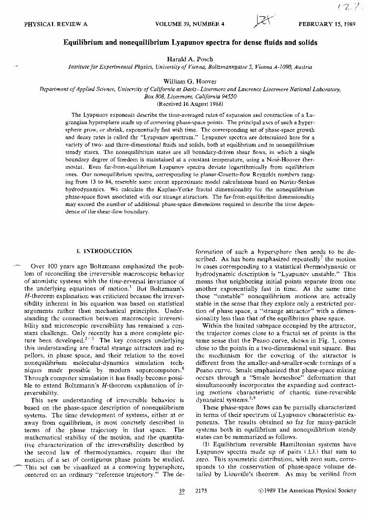
Within the limited subspace occupied by the attractor the trajector comes close to a fractal set of points in the same sense that the Peano curve shown in Fig 1 comes close to the points in a two-dimensional unit square But the mechanism for the covering of the attractor is different from the smaller-and-smaller-scale turnings of a Peano curve Smale emphasized that phase-space mixing occurs through a Smale horseshoe deformation that simultaneously incorporates the expanding and contractshying motions characteristic of chaotic time-reversible dynamical systems89
These phase-space flows can be partially characterized in terms of their spectrum of Lyapunov characteristic exshyponents The results obtained so far for many-particle systems both in equilibrium and nonequilibrium steady states can be summarized as follows
(1) Equilibrium reversible Hamiltonian systems have Lyapunov spectra made up of pairs ( that sum to zero This symmetric distribution with zero sum correshysponds to the conservation of phase-space volume deshytailed by Liouvilles theorem As may be verified from
39 2175 1989 The American Physical Society
2176 HARALD A POSCH AND WILLIAMG HOOVER 39
t t
t t
Peano Smale
FIG 1 The Peano space-filling curve and the Smale horseshoe
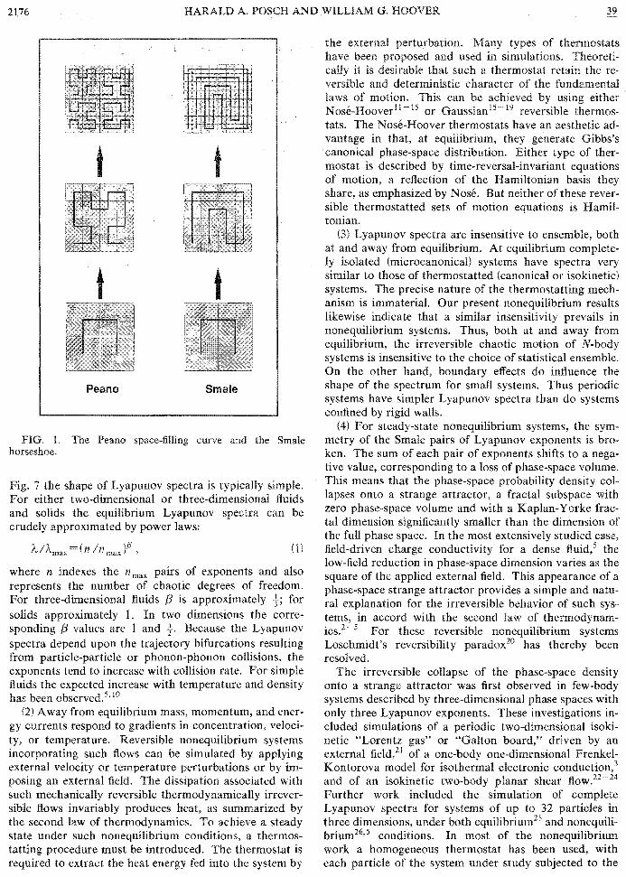
7 the shape of Lyapunov spectra is typically simple For either two-dimensional or three-dimensional fluids and solids the equilibrium Lyapunov spectra can be crudely approximated by power laws
where n indexes the n max pairs of exponents and also represents the number of chaotic degrees of freedom For three-dimensional fluids 3 is approximately t for solids approximately I In two dimensions the correshysponding 3 values are 1 and f Because the Lyapunov spectra depend upon the trajectory bifurcations resulting from particle-particle or phonon-phonon collisions the exponents tend to increase with collision rate For simple fluids the expected increase with temperature and density has been observed 510
(2) Away from equilibrium mass momentum and enershygy currents respond to gradients in concentration velocishyty or temperature Reversible nonequiIibrium systems incorporating such flows can be simulated by applying external velocity or temperature perturbations or by imshyposing an external field The dissipation associated with such mechanically reversible thermodynamically irrevershysible flows invariably produces heat as summarized by the second law of thermodynamics To achieve a steady state under such nonequilibrium conditions a thermosshytatting procedure must be introduced The thermostat is required to extract the heat energy fed into the system by
the external perturbation Many types of thermostats have been proposed and used in simulations Theoretishycally it is desirable that such a thermostat retain the reshyversible and deterministic character of the fundamental laws of motion This can be achieved by eithermiddot Nose-Hooverll- 15 or Gaussian15
-19 reversible thermosshy
tats The Nose-Hoover thermostats have an aesthetic adshyvantage in that at equilibrium they generate Gibbss canonical phase-space distribution Either type of thershymostat is described by time-reversal-invariant equations of motion a reflection of the Hamiltonian basis they share as emphasized by Nose But neither of these revershysible thermostatted sets of motion equations is Hamilshytonian
(3) Lyapunov spectra are insensitive to ensemble both at and away from equilibrium At equilibrium completeshyly isolated (microcanonicaD systems have spectra very similar to those of thermostatted (canonical or isokinetic) systems The precise nature of the thermostatting mechshyanism is immaterial Our present nonequilibrium results likewise indicate that a similar insensitivity prevails in nonequilibrium systems Thus both at and away from equilibrium the irreversible chaotic motion of N-body systems is insensitive to the choice of statistical ensemble On the other hand boundary effects do influence the shape of the spectrum for small systems Thus periodic systems have simpler Lyapunov spectra than do systems confined by rigid walls
(4) For steady-state nonequilibrium systems the symshymetry of the Smale pairs of Lyapunov exponents is broshyken The sum of each pair of exponents shifts to a negashytive value corresponding to a loss of phase-space volume This means that the phase-space probability density colshylapses onto a strange attractor a fractal subspace with zero phase-space volume and with a Kaplan-Yorke fracshytal dimension significantly smaller than the dimension of the full phase space In the most extensively studied case field-driven charge conductivity for a dense fluidS the low-field reduction in phase-space dimension varies as the square of the applied external field This appearance of a phase-space strange attractor provides a simple and natushyral explanation for the irreversible behavior of such sysshytems in accord with the second law of thermodynamshy
5ics2 - For these reversible nonequilibrium systems Loschmidts reversibility paradox2o has thereby been resolved
The irreversible collapse of the phase-space density onto a strange attractor was first observed in few-body systems described by three-dimensional phase spaces with only three Lyapunov exponents These investigations inshycluded simulations of a periodic two-dimensional isokishynetic Lorentz gas or Galton board driven by an external field1 of a one-body one-dimensional FrenkelshyKontorova model for isothermal electronic conduction3
22 24and of an isokinetic two-body planar shear flOW shy
Further work included the simulation of complete Lyapunov spectra for systems of up to 32 particles in three dimensions under both equilibrium25 and nonequilishybrium26
bull5 conditions In most of the nonequilibrium
work a homogeneous thermostat has been used with each particle of the system under study subjected to the
2177 EQUILIBRIUM AND NONEQUILIBRIUM L Y APUNOV SPECTRA
thermostatting constraint force Both Nose-Hoover thershymostats characterized by a response time I and Gaussshyian thermostats corresponding to the limit have been employed
Closer to experiment and therefore of more inshyterest are the boundary-bulk-boundary nonequilibrium systems as indicated schematically in Fig 2 and investishygated earlier2724 Such systems may incorporate two or more boundary regions in which particles interact with an external force and a thermostat with a bulk region sandwiched between the boundaries In the bulk Newtonian regions the particle motion is solely governed by Newtons equations of motion In the heat-flow case with the geometry illustrated in Fig 3 the boundary reshygions on the left and right represent hot and cold resershyvoirs The heat transported through the Newtonian bulk system can then be studied4
In this paper we present the results of extensive simulashytions of two-dimensional shear flow (plane Couette flow) for systems of N two- or three-dimensional bulk Newtonian particles A typical situation is sketched in Fig 3 The bulk particles are enclosed by a downmoving vertical boundary to the left and an upmoving vertical boundary on the right with periodic boundaries linking the top and bottom of the system By fixing the normal separation of the two moving boundaries to a constant value it is possible to describe their horizontal (x) motion with a single degree of freedom thermostatted by a single Nose-Hoover thermostat This model evolved so as to minimize the boundary and thermostat degrees of freeshydom and is described in more detail in the following secshytion A modified two-dimensional shear model with two boundary degrees of freedom is discussed in Sec VI A Extensions to shear flow in three dimensions are treated in Sec VI C
The method for determining the model Lyapunov specshytra is discussed in Sec II Our simulation results for sysshytems involving up to N 81 bulk particles in two dimenshysions and N =27 particles in three dimensions are all reshyported in Secs III-VI As detailed in Secs IV and VI
Cold
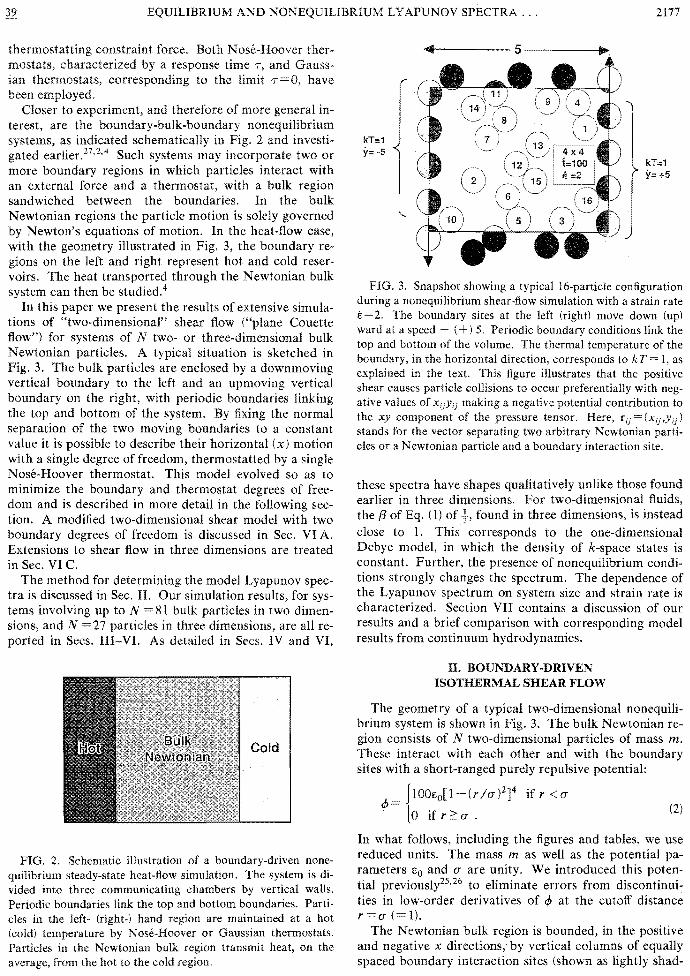
FIG 2 Schematic illustration of a boundary-driven noneshyquilibrium steady-state heat-flow simulation The system is dishyvided into three communicating chambers by vertical walls Periodic boundaries link the top and bottom boundaries Partishycles in the left- (right-) hand region are maintained at a hot (cold) temperature by Nose-Hoover or Gaussian thermostats Particles in the Newtonian bulk region transmit heat on the average from the hot to the cold region
kT=1 y= -5
kT=1 y= +5
FIG 3 Snapshot showing a typical 16-particle configuration during a nonequilibrium shear-flow simulation with a strain rate 1=2 The boundary sites at the left (right) move down (up) ward at a speed (+) 5 Periodic boundary conditions link the top and bottom of the volume The thermal temperature of the boundary in the horizontal direction corresponds to kT = 1 as explained in the text This figure illustrates that the positive shear causes particle collisions to occur preferentially with negshyative values of XiJYij making a negative potential contribution to the xy component of the pressure tensor Here r ij = (x ijy ij )
stands for the vector separating two arbitrary Newtonian partishycles or a Newtonian particle and a boundary interaction site
these spectra have shapes qualitatively unlike those found earlier in three dimensions For two-dimensional fluids the l3 of Eq (1) of found in three dimensions is instead close to 1 This corresponds to the one-dimensional Debye model in which the density of k-space states is constant Further the presence of nonequilibrium condishytions strongly changes the spectrum The dependence of the Lyapunov spectrum on system size and strain rate is characterized Section VII contains a discussion of our results and a brief comparison with corresponding model results from continuum hydrodynamics
n BOUNDARY-DRIVEN ISOTHERMAL SHEAR FLOW
The geometry of a typical two-dimensional nonequilishybrium system is shown in Fig 3 The bulk Newtonian reshygion consists of N two-dimensional particles of mass m These interact with each other and with the boundary sites with a short-ranged purely repulsive potential
JlOOEo[ 1 - (r I a 2]4 if r lt a
lo if r a (2)
In what follows including the figures and tables we use reduced units The mass m as well as the potential pashyrameters EO and a are unity We introduced this potenshytial previously2526 to eliminate errors from discontinuishyties in low-order derivatives of cp at the cutoff distance r =a ( 1)
The Newtonian bulk region is bounded in the positive and negative x directions by vertical columns of equally spaced boundary interaction sites (shown as lightly shadshy
2178 HARALD A POSCH AND WILLIAM G HOOVER
ed in Fig 3) These boundary sites are arranged parallel to the vertical (y) axis The spacing between adjacent boundary sites (T (= 1) is equal to the potential cutoff distance There are L I (T interaction sites for each boundary L is the periodicity interval for the periodic boundary conditions applied in the vertical direction The horizontal (x) spacing between centers of the two columns of sites is kept constant and equal to L + (T In all simulations L was chosen to be equal to liN (T thus fixing the number density N IL2 of the Newtonian bulk particles at 1 All of the boundary sites are coherently joined together so that their horizontal momentum reacts to the summed interactions of all of the bulk partishycles which lie within unit distance of any boundary site The total mass associated with the x motion of the boundary sites is unity the same as the mass of a single Newtonian bulk particle The thermodynamic temperashyture associated with the boundary sites is also taken to be unity and is enforced by a Nose-Hoover thermostat which guarantees on a time-averaged basis that the flucshytuating part of the boundary kinetic energy P 12m has the equipartition value t
(3)
Here is the momentum in the x direction of all 2L boundary sites with a combined mass equal to the mass m 1 of a Newtonian particle ( gt denotes a time average k is Boltzmanns constant and T is the average temperature of this horizontal boundary degree of freeshydom No thermal fluctuations of the boundary motion in the vertical (y) direction are allowed In this direction the boundary particles move with a constant velocity VB related to the imposed strain rate eby
+(T)e (4)
where the plus and minus signs refer to the right- and left-hand columns of boundary sites respectively It is sufficient to solve the equations of motion for a single boundary site by properly adding all interactions linking bulk and boundary particles using appropriate periodic boundary conditions in the y direction We denote the position of this reference site by R = (X Y) and its flucshytuating momentum by P=(PxO) The positions of an arshybitrary boundary particle are given by RB = (XB YB ) If furthermore TnPn denote the respective positions and momenta of the bulk particles (n 12 N) then the equations of motion of our model system take the form
Til =Pn 1m
(5) (L+(T)e2
ix -altPintaX -tPx
~=(PlmkT-l)
Here ~N is the potential energy of the Newtonian bulk (assumed to be pairwise additive) and ltPint is the interacshy
tion energy between the Newtonian particles and the moving walls
ltPN= ~ ~ 1gt( irn-rlll) n ( fl) n
(6) ltPnt= ~ ~ 1gt( Irn-R B )
B n
The sum over B is over all 2L I (T interactions sites of the boundary
Extension of this model to three dimensions is straightshyforward Either spherical or cylindrical boundary partishycles can be used We have chosen cylinders to avoid inshyducing motion in the z direction This model is discussed in more detail in Sec VI C
The thermostat variable t which causes the boundary momentum to fluctuate on a timescale T in the x direcshytion is an independent variable arising as a momentum in Noses original derivation Thus in two (three) dimenshysions the dimensionality of the phase space is increased from the bulk-particle value of 4N (6N) to 4N +4 (6N +4) including the x coordinate and momentum of the boundary reference site its y coordinate and the fricshytion coefficient t The dimension of the phase space is of crucial importance in the description and discussion of the results of our simulations
Let the flow equations (5) be abbreviated by
(7)
where r (rnPnXPx Yt) is a (4N +4)-dimensional state vector In principle the 4N +4 Lyapunov exshyponents are calculated by solving-in addition to (7)-the 4N +4 linearized sets of equations28 - 32
(8)
where I 12 4N +4 for the two-dimensional case D(r)=aG(r)ar is a quadratic dynamical matrix which couples the reference trajectory to the differenshytially separated satellite trajectories represented by 8(t) An arbitrarily oriented set of orthonormal vectors can serve as initial condition for the vectors 8[ (t) In the course of time these vectors do not stay orthonormal but tend to rotate into the direction of maximum phase-space growth By application of a Gram-Schmidt orthonormalshyization procedure every few time steps one finds that the vector 81 tends to point uniquely into a direction of most rapid phase space growth [proportional to exp(j t)] Similarly 8182 span a subspace whose area grows most rapidly [proportional to exp( Ai + A)t] and so forth From this sequence all Ai are obtained The Lyapunov exponents are the time averages of these quantities
(9)
In practice we follow the trajectories forward for a time t of the order of 1000 employing a fourth-order Runge-Kutta integration scheme To avoid initial transhysients we exclude the first 30 of the trajectory from the averaging procedure For almost all simulation results we report in the following sections a reduced time step
39 EQUILIBRIUM AND NONEQUILIBRIUM L Y APUNOV SPECTRA 2179
At =0001 is used all exceptions being specially marked at the appropriate places
The sum over all Lyapunov exponents (~A) is equal to the averaged logarithmic rate of growth of the phaseshyspace volume In our case this means that
(10)
where as in (9) lt ) denotes a time average (in practice over the length l of the run) The quantity A =d alar) t(t) is called the phase-space compressibility The sum rule (10) provides a convenient test for the conshysistency of our simulation results Typically (10) is fulfilled to an accuracy of at least four significant digits
The internal energy of our boundary-bulk-boundary shear problem (5) is given by
Making use of the equations of motion the rate of change ofH(r) is given by
aH rmiddot = (12)ar where
(13)
The sum in the last equation is over all boundary interacshytion sites and YB is given by (4) Since altlgtintaYB is the total frictional force component parallel to the shear exshyerted by the boundary site B on the bulk W( r) is the rate of work performed on the system by the boundary The first term on the right-hand side of (12) is the rate at which heat is extracted by the thermostat In nonequilishybrium steady states both terms cancel each other (inn) =0 from which we find a quadratic strain-rate dependence of the averaged friction (s)
(14)
In this equation 7 is the viscosity defined by
(15)
The factor 2 accounts for the total length of the comshybined left and right boundaries Equation (14) is used to obtain 7J from the simulation results for (s)middot
Integrating (12) one finds that the quantity
(16)
is constant along a trajectory r(t) both at equilibrium (for which W vanishes) as well as in nonequilibrium states We have verified that HNose is indeed conserved by our simulations However the total momentum of the boundary-bulk-boundary system is not a constant of the motion 13 The consequences are discussed in Sec III
The information-theory entropy is defined by
Sinf=-k Jdr j(rt)lnj(rt) (17)
where j (r t) is the phase-space distribution function Equating time averages with ensemble averages over the non equilibrium ensemble one finds for the rate of change of Sinf (Refs 33 and 34)
(18)
For non equilibrium steady-state conditions the rate of change of Sinf is balanced by the rate of (global) irreversishyble entropy production
(19)
which according to (14) is a positive quadratic function of the applied strain rate t
The thermostat response time T enters the Nose equashytions of motion as a free parameter In what follows we require that T is proportional to the mean collision time between bulk particles and the boundary Because in two dimensions the respective collision rate is proportional to the periodicity interval in the y direction L we choose T= IlL (in our reduced units) In three dimensions T= 1L 2 The Lyapunov spectra reported in the followshying sections are insensitive to this choice Furthermore the boundary thermostat temperature T chosen for all our simulations corresponds to kT = 1
The linear differential equation for Yin (5) is associated with a vanishing Lyapunov exponent From a practical point of view it is advantageous to avoid the timeshyconsuming computation of this vanishing exponent in an ordered sequence Ai Ai + I as required by the algoshyrithms This can be achieved by replacing this trivial differential equation by its integral Y(t)= Vt + Y(O) and using Y(t) for the evaluation of ltlgtint This converts the autonomous system of flow equations (5) with (4N +4)dimensional phase space into a non autonomous system of order 4N + 3 and reduces the number of exshyponents to be calculated by one In three dimensions 4N is replaced by 6N
At relatively high strain rates the kinetic energy of some Newtonian particles might become large enough to overcome the potential barrier imposed by the walls In this case a Newtonian particle can escape by slipping beshytween two neighboring boundary interaction sites In our first runs we were alerted to this problem by noticing that pairs of Lyapunov exponents started to vanish two pairs for each escaped particle We then prevented such esshycapes by imposing an elastic reflection whenever a bulk particle attempted to cross the boundary lines x =X and x = X + L + a respectively
III MAXIMUM LYAPUNOV EXPONENTS
The maximum Lyapunov exponent Amax reflects the rate of the fastest dynamical events taking place in phase space In Table I this quantity is listed for the twoshydimensional simulations for various system sizes N both at equilibrium (t=O) as well as in nonequilibrium steady states Also given in this table is the time-averaged thershy
2180 HARALD A POSCH AND WILLIAM G HOOVER 39
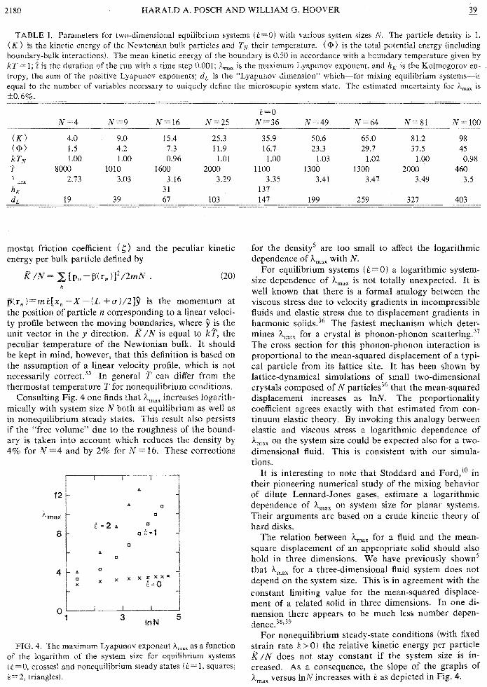
TABLE I Parameters for two-dimensional equilibrium systems (t=o) with various system sizes N The particle density is 1 ltK) is the kinetic energy of thc Newtonian bulk particles and TN their temperature lt1raquo is the total potential energy (including boundary-bulk interactions) The mean kinetic energy of the boundary is 050 in accordance with a boundary temperature given by kT = 1 tis the duration of the run with a time step 0001 max is the maximum Lyapunov exponent and 11K is the Kolmogorov enshytropy the sum of the positive Lyapunov exponents is the Lyapullov dimension which-for mixing equilibrium systems-i~ equal to the number of variables necessary to uniquely define the microscopic system state The estimated uncertainty for Amax is plusmn06
N=4 N=9 N 25 =o
N=36 N=49 N=64 N=81 N 100
(K) lt1gt )
1 ~
x
hK
40 15 100
8000 273
19
90 42 100
1010 303
39
154 73 096
1600 316
31 67
253 119 101
2000 329
103
359 167 100
1100 335
137 147
506 233
103 1300
341
199
650 297
102 1300
347
259
812 375
100 2000
349
327
98 45
098 460
35
403
mostat friction coefficient (s) and the peculiar kinetic energy per bulk particle defined by
(20)
p(Tn )=mpound[xn - X -L +cr )2]51 is the momentum at the position of particle n corresponding to a linear velocishyty profile between the moving boundaries where y is the unit vector in the y direction K 11 is equal to the peculiar temperature of the Newtonian bulk It should be kept in mind however that this definition is based on the assumption of a linear velocity profile which is not necessarily correct 35 In general l can differ from the thermostat temperature T for nonequilibrium conditions
Consulting Fig 4 one finds that )max increases logarithshymically with system size 11 both at equilibrium as well as in non equilibrium steady states This result also persists if the free volume due to the roughness of the boundshyary is taken into account which reduces the density by 4 for 11 =4 and by 2 for 11 16 These corrections
12 CI
Amax CI
E CI2
o E=18 CI
A CI
4
3 5InN
FIG 4 The maximum Lyapunov exponent Amax as a function of the logarithm of the system size for equilibrium systems (t=O crosses) and nonequilibrium steady states (1=1 squares =2 triangles)
for the density5 are too small to affect the logarithmic dependence of Amax with 11
For equilibrium systems (pound=0) a logarithmic systemshysize dependence of Ama is not totally unexpected It is well known that there is a formal analogy between the viscous stress due to velocity gradients in incompressible fluids and elastic stress due to displacement gradients in harmonic solids36 The fastest mechanism which detershymines Amax for a crystal is phonon-phonon scattering37
The cross section for this phonon-phonon interaction is proportional to the mean-squared displacement of a typishycal particle from its lattice site It has been shown by lattice-dynamical simulations of small two-dimensional crystals composed of N particles36 that the mean-squared displacement increases as InN The proportionality coefficient agrees exactly with that estimated from conshytinuum elastic theory By invoking this analogy between elastic and viscous stress a logarithmic dependence of Amax on the system size could be expected also for a twoshydimensional fluid This is consistent with our simulashytions
It is interesting to note that Stoddard and Ford1O in their pioneering numerical study of the mixing behavior of dilute Lennard-Jones gases estimate a logarithmic dependence of Amax on system size for planar systems Their arguments are based on a crude kinetic theory of hard disks
The relation between Amax for a fluid and the meanshysquare displacement of an appropriate solid should also hold in three dimensions We have previously shown5
that Amax for a three-dimensional fluid system does not depend on the system size This is in agreement with the constant limiting value for the mean-squared displaceshyment of a related solid in three dimensions In one dishymension there appears to be much less number depenshydence 38 39
For nonequilibrium steady-state conditions (with fixed strain rate tgt 0) the relative kinetic energy per particle K 11 does not stay constant if the system size is inshycreased As a consequence the slope of the graphs of
versus InN increases with pound as depicted in Fig 4
2181 EQUILIBRIUM AND NONEQUILIBRIUM L Y APUNOV SPECTRA
An interesting but unexpected phenomenon takes place for larger strainrates (t 2) and large enough systems (N gt 36) It has been mentioned already in Sec II that the equations of motion (5) do not conserve the total momentum of the boundary-bulk-boundary system
d -~Px (21)
dt [~Pn +P] = - ~ altlgtintaYn n J
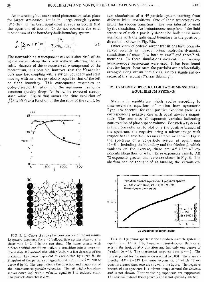
The nonvanishing x component causes a slow drift of the whole system along the x axis without affecting the reshysults Because of the non conserved Y component of the momentum it is possible however that the Newtonian bulk may lose coupling with a system boundary and start moving with an average velocity equal to that of the left or right boundary This consequence resembles an order-disorder transition and the maximum Lyapunov exponent quickly drops far below its expected steadyshystate value Figure Sea) shows the time evolution of f1A( tldt It as a function of the duration of the run t for
OL-_-~~L_~~~~_~---~
o 500 1000 1500
FIG 5 (al Curve A shows the convergence of the maximum Lyapunov exponent for a 49-bulk-particle system sheared at a shear rate pound=2 1 is the run time The same system with different initial conditions suffers a transition into a more orshydered state at 1 around 400 which leads to a fast decrease of the maximum Lyapunov exponent as exemplified by curve B (bl Snapshot of the particle configuration at a run time 1= 1500 of curve B in (a) The bars indicate the direction and magnitude of the instantaneous particle velocities The left (right) boundary moves down (up) with a velocity equal to 8 in reduced units The particle diameter is a 1
two simulations of a 49-partic1e system starting from different initial conditions One of these trajectories exshyhibits this sudden transition in the time interval covered by the simulation An instantaneous snapshot of the fluid structure of such a partially decoupled bulk phase movshying along with the right-hand boundary in the positive Y direction is shown in Fig S(b)
Other kinds of order-disorder transitions have been obshyserved recently in nonequilibrium molecular-dynamics simulations of shear flow both in tw040 and three41 dishymensions In these simulations momentum-conserving homogeneous thermostats were used It has been found that for larger shear rates the particles are preferentially arranged along stream lines giving rise to a significant deshycrease of the viscosity (shear thinning)
IV LYAPUNOV SPECTRA FOR TWO-DIMENSIONAL EQUILIBRIUM SYSTEMS
Systems in equilibrium which evolve according to time-reversible equations of motion have symmetric Lyapunov spectra for each positive exponent there is a corresponding negative one with equal absolute magnishytude The sum over all exponents vanishes indicating conservation of phase-space volume For such a system it is therefore sufficient to plot only the positive branch of the spectrum the negative being a mirror image with respect to the abscissa As an example we show in Fig 6 the spectrum of a 36-partic1e system at equilibrium (pound=0) Including the boundary and the friction ~ which vanishes on the average there are 4N +3 147 exshyponents altogether of which three exponents vanish All 72 exponents greater than zero are shown in Fig 6 The abscissa can be thought of as labeling the various exshy
FIG 6 Lyapunov spectrum for a 36-bulk-partic1e system in equilibrium (pound=0) The boundary Nose-Hoover thermostat acts in the horizontal x direction and has only one degree of freedom (g I) The thermostat response time is 1= i The time step used for the simulation is equal to 0001 There are alshytogether 4N +3= 147 Lyapunov exponents of which 72 exshyponents greater than zero are shown in the figure The negative branch of the spectrum is a mirror image around the abscissa and is not shown Four vanishing exponents are suppressed The abscissa indexes the exponents and is not specially labeled
2182 HARALD A POSCH AND WILLIAM G HOOVER 39
ponents by a Lyapunov index n with n = I for the smallshyest positive exponent and n =72 for the top-right maxshyimum exponent Amax The index n (A) can be interpreted as the number of positive exponents less or equal to A Parameters related to this spectrum are also contained in Table I
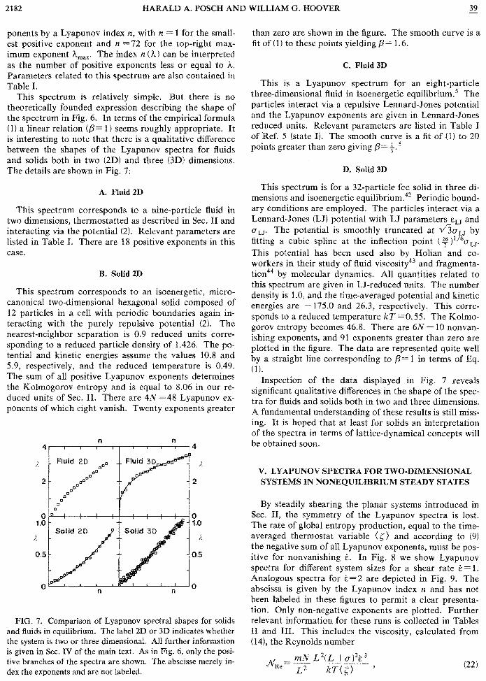
This spectrum is relatively simple But there is no theoretically founded expression describing the shape of the spectrum in Fig 6 In terms of the empirical formula (1) a linear relation (3= 1) seems roughly appropriate It is interesting to note that there is a qualitative difference between the shapes of the Lyapunov spectra for fluids and solids both in two (2D) and three (3D) dimensions The details are shown in Fig 7
A Fluid 2D
This spectrum corresponds to a nine-particle fluid in two dimensions thermostatted as described in Sec II and interacting via the potential (2) Relevant parameters are listed in Table I There are 18 positive exponents in this case
B Solid 2D
This spectrum corresponds to an isoenergetic microshycanonical two-dimensional hexagonal solid composed of 12 particles in a cell with periodic boundaries again inshyteracting with the purely repulsive potential (2) The nearest-neighbor separation is 09 reduced units correshysponding to a reduced particle density of 1426 The poshytential and kinetic energies assume the values 108 and 59 respectively and the reduced temperature is 049 The sum of all positive Lyapunov exponents determines the Kolmogorov entropy and is equal to 806 in our reshyduced units of Sec II There are 4N =48 Lyapunov exshyponents of which eight vanish Twenty exponents greater
n n 44
Fluid 2D )) 0dega 0 0
0 0
0 02 20
0 0
0 a a
0 0
o a 0 10 10
Solid 2D )(
05 05
0 0 n n
FIG 7 Comparison of Lyapunov spectral shapes for solids and fluids in equilibrium The label 2D or 3D indicates whether the system is two or three dimensional All further information is given in Sec IV of the main text As in Fig 6 only the posishytive branches of the spectra are shown The abscisse merely inshydex the exponents and are not labeled
than zero are shown in the figure The smooth curve is a fit of (1) to these points yielding 3= 1 6
C Fluid 3D
This is a Lyapunov spectrum for an eight-particle three-dimensional fluid in isoenergetic equilibrium 5 The particles interact via a repulsive Lennard-Jones potential and the Lyapunov exponents are given in Lennard-Jones reduced units Relevant parameters are listed in Table I of Ref 5 (state I) The smooth curve is a fit of (1) to 20 points greater than zero giving -5
D Solid 3D
This spectrum is for a 32-particle fcc solid in three dishymensions and isoenergetic equilibrium42 Periodic boundshyary conditions are employed The particles interact via a Lennard-Jones (LJ) potential with LJ parameters ELJ and aLJ The potential is smoothly truncated at V3aLJ by fitting a cubic spline at the inflection point (yen )1I6aLJ
This potential has been used also by Holian and coshyworkers in their study of fluid viscosity43 and fragmentashytion44 by molecular dynamics All quantities related to this spectrum are given in LJ-reduced units The number density is 10 and the time-averaged potential and kinetic energies are 1750 and 263 respectively This correshysponds to a reduced temperature kT =0 55 The Kolmoshygorov entropy becomes 468 There are 6N - 10 nonvanshyishing exponents and 91 exponents greater than zero are plotted in the figure The data are represented quite well by a straight line corresponding to 3= I in terms of Eq (1)
Inspection of the data displayed in Fig 7 reveals significant qualitative differences in the shape of the specshytra for fluids and solids both in two and three dimensions A fundamental understanding of these results is still missshying It is hoped that at least for solids an interpretation of the spectra in terms of lattice-dynamical concepts will be obtained soon
V LYAPUNOV SPECTRA FOR TWOmiddotDIMENSIONAL SYSTEMS IN NONEQUILIBRIUM STEADY STATES
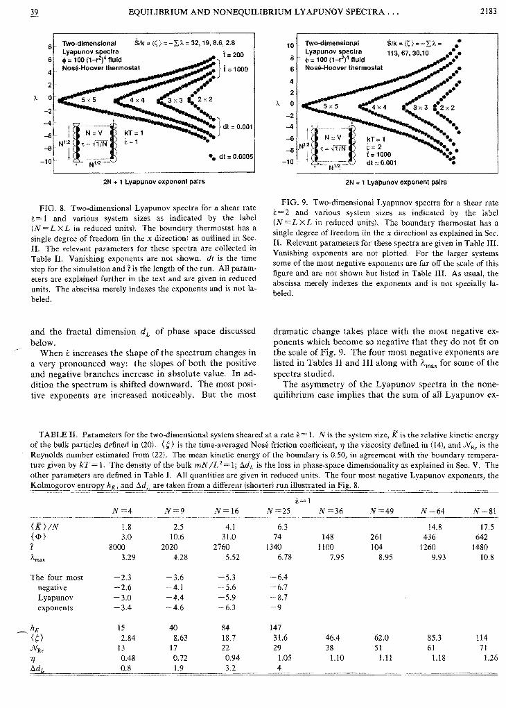
By steadily shearing the planar systems introduced in Sec II the symmetry of the Lyapunov spectra is lost The rate of global entropy production equal to the timeshyaveraged thermostat variable (() and according to (9) the negative sum of all Lyapunov exponents must be posshyitive for nonvanishing t In Fig 8 we show Lyapunov spectra for different system sizes for a shear rate t= 1 Analogous spectra for t = 2 are depicted in Fig 9 The abscissa is given by the Lyapunov index n and has not been labeled in these figures to permit a clear presentashytion Only non-negative exponents are plotted Further relevant information for these runs is collected in Tables II and III This includes the viscosity calculated from (14) the Reynolds number
N =mNf2(L+a)2t 3
(22)Re L2 kT()
39 EQUILIBRIUM AND NONEQUILIBRIUM LY APUNOV SPECTRA 2183
Two-dimensional Sik =(I ) = - L A= Lyapunov spectra 113673010 p = 100 1_r2)4 fluid Nose-Hoover thermostat
kT= 1 E= 2 1=1000 dt 0001
2N + 1 Lyapunov exponent pairs
FIG 8 Two-dimensional Lyapunov spectra for a shear rate t = 1 and various system sizes as indicated by the label (N = LX L in reduced units) The boundary thermostat has a single degree of freedom (in the x direction) as outlined in Sec II The relevant parameters for these spectra are collected in Table II Vanishing exponents are not shown dt is the time step for the simulation and tis the length of the run All paramshyeters are explained further in the text and are given in reduced units The abscissa merely indexes the exponents and is not lashybeled
and the fractal dimension dL of phase space discussed below
When increases the shape of the spectrum changes in a very pronounced way the slopes of both the positive and negative branches increase in absolute value In adshydition the spectrum is shifted downward The most posishytive exponents are increased noticeably But the most
TABLE II Parameters for the two-dimensional system sheared at a rate E= L N is the system size K is the relative kinetic energy of the bulk particles defined in (20) lt~ gt is the time-averaged Nose friction coefficient 7J the viscosity defined in (14) and N Re is the Reynolds number estimated from (22) The mean kinetic energy of the boundary is 050 in agreement with the boundary temperashyture given by kT = 1 The density of the bulk mNIL 2= 1 tdL is the loss in phase-space dimensionality as explained in Sec V The other parameters are defined in Table I All quantities are given in reduced units The four most negative Lyapunov exponents the
and
N=4
(KIN 18 ltltP gt 30 t 8000 max 329
The four most -23 negative -26 Lyapunov -30 exponents -34
hK-lt0
15 284
N Re 13
7J 048 08
2N + 1 Lyapunov exponent pairs
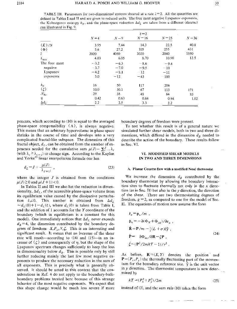
FIG 9 Two-dimensional Lyapunov spectra for a shear rate I = 2 and various system sizes as indicated by the label (N = L XL in reduced units) The boundary thermostat has a single degree of freedom (in the x direction) as explained in Sec II Relevant parameters for these spectra are given in Table III Vanishing exponents are not plotted For the larger systems some of the most negative exponents are far off the scale of this figure and are not shown but listed in Table Ill As usual the abscissa merely indexes the exponents and is not specially lashybeled
dramatic change takes place with the most negative exshyponents which become so negative that they do not fit on the scale of Fig 9 The four most negative exponents are listed in Tables II and III along with max for some of the spectra studied
The asymmetry of the Lyapunov spectra in the noneshyquilibrium case implies that the sum of all Lyapunov ex-
are taken from a different run illustrated in 8
t=1 N=9 N=16 N=25 N=36
~~---~------~-----
25 41 63 106 310 74 148
2020 2760 1340 1100 428 552 678 795
-36 -53 -64 -41 -56 -67 -44 -59 -87 -46 -63 -9
40 84 147 863 187 316 464
17 22 29 38 072 094 105 110 19 32 4
N=49 N=64 N=81
148 175 261 436 642 104 1260 1480
895 993 108
620 853 114 51 61 71
111 118 126
2184 HARALD A POSCH AND WILLIAM G HOOVER 39
TABLE III Parameters for two-dimensional systems sheared at a rate E = 2 All the quantities are defined in Tables I and II and are given in reduced units The four most negative Lyapunov exponents the Kolmogorov entropy hK and the phase-space reduction 1dL are taken from a different (shorter) run illustrated in Fig 9
ponents which according to (10) is equal to the averaged phase-space compressibility ltA) is always negative This means that an arbitrary hypervolume in phase space shrinks in the course of time and develops into a very complicated fractal-like subspace The dimension of this fractal object dL can be obtained from the number of exshyponents needed for the cumulative sum f1(J)= Lf=l Ai (with Ai 2 Ai +1) to change sign According to the Kaplan and Y orke45 linear interpolation formula one has
_ f1(J) (23)dL -J +-IA--I
J+l
where the integer J is obtained from the conditions f1(J) 2 degand f1(J + 1) lt 0
In Tables II and III we also list the reduction in dimenshysionality J1dv of the accessible phase-space volume from its equilibrium value caused by the dissipative perturbashytion pound0 This number is obtained from J1dL
=dL(O)+ I-dL(pound) where dL(O) is taken from Table I and the addition of 1 accounts for the Y coordinate of the boundary (which in equilibrium is a constant for this model) One immediately notices that J1dL never exceeds dB =4 the dimension contributed by the boundary deshygrees of freedom XPx Ys This is an interesting and significant result It means that an increase of the shear rate will result-according to (4) and (15)-in an inshycrease of lts) and consequently of 7] but the shape of the Lyapunov spectrum changes sufficiently to keep the loss in dimensionality below dB This is possible only by still further reducing mainly the last few most negative exshyponents to produce the necessary reduction in the sum of all exponents This is precisely what is generally obshyserved It should be noted in this context that the conshysiderations in Ref 4 do not apply to the boundary-bulkshyboundary problems treated here because of this strange behavior of the most negative exponents We expect that this shape change would be much less severe if more
boundary degrees of freedom were present To test whether this result is of a general nature we
simulated further shear models both in two and three dishymensions which differed in the dimension dB needed to describe the action of the boundary These results follow in Sec VI
VI MODIFIED SHEAR MODELS IN TWO AND THREE DIMENSIONS
A Planar Couette flow with a modified Nose thermostat
We increase the dimension dB contributed by the boundary thermostat by allowing the boundary interacshytion sites to fluctuate thermally not only in the x direcshytion (as in Sec IV but also in the y direction the direction of the shear There are two thermostatting degrees of freedom g = 2 as compared to one for the model of Sec II The equations of motion now assume the form
Pn = -a(ltPN+ltPint)arn
R=Plm -f(L +a)poundy (24)
p= -altIgtint aR -sP t=(p2I2mkT-l)h2
As before R = (X Y) denotes the position and P =(Px Py ) the thermally fluctuating part of the momenshytum for the boundary reference site y is the unit vector in y direction The thermostat temperature is now detershymined by
kT=(P+P)2m (25)
instead of (3) and the sum rule 00) takes the form
2185 AND NONEQUILIBRIUM L Y APUNOV SPECTRA
(26)
where A is the sum over all exponents In practice this equation for a 16-particle system is obeyed with a precision- of at least five significant figures after 300000 time steps
Similar to (16) the quantity
P~ p2 HNose(rJ=ltlgtN+ltlgtint + 2 2 + 2 +
m m
- ftW(rJdt+gkT ffdt (27) o 0
(g =2) is a constant along the trajectory r(t) where W by (13) is the rate at which work is performed on
the system by the boundary The value of depends on the choice of the time origin We have verified that (27) is conserved by our simulations As in the shear model of Sec II the total momentum is not a constant of the motion
4N +5 variables are needed to characterize uniquely the state vector r = (rn Pn R P () of the system Conseshyquently the equilibrium phase-space dimension dL (0)
4N +5 The reduction in phase-space dimensionality due to the dissipative perturbation is given by tdL =4N +5-dL (pound) The dimension contributed by the boundary degrees of freedom is dB = 5
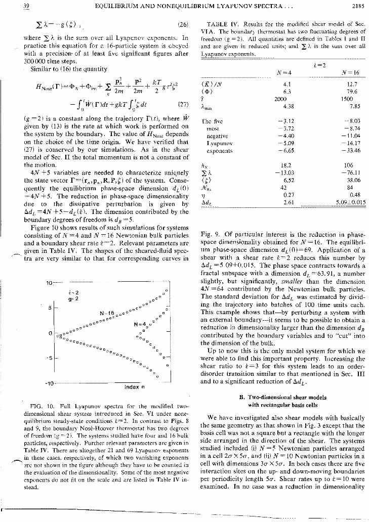
Figure 10 shows results of such simulations for systems consisting of N =4 and N = 16 Newtonian bulk particles and a boundary shear rate t = 2 Relevant parameters are given in Table IV The shapes of the sheared-fluid specshy
~
tra are very similar to that for corresponding curves in
Index n
FIG 10 Full Lyapunov spectra for the modified twoshydimensional shear system introduced in Sec VI under noneshyquilibrium steady-state conditions pound=2 In contrast to Figs 8 and 9 the boundary Nose-Hoover thermostat has two degrees of freedom (g =2) The systems studied have four and 16 bulk particles respectively Further relevant parameters are given in Table IV There are altogether 21 and 69 Lyapunov exponents
~in these cases respectively of which two vanishing exponents Ire not shown in the although they have to be counted in the evaluation of the dimensionality Some of the most negative exponents do not fit on the scale and are listed in Table IV inmiddotmiddot stead
TABLE IV Results for the modified shear model of Sec VI A The boundary thermostat has two fluctuating of freedom (g 2) All quantities are defined in Tables I and II
in reduced units and 2 f is the sum over all
pound=2 N=4 N 16
(K)IN 41 127 ( ltlgt ) 63 796 t 2000 1500
Amax 438 785
The five -312 -803 most 372 -874 negative -440 -1104 Lyapunov 509 -1417 exponents 665 3346
hK 182 106 2 I 1303 -7611 (sgt 652 3806 NRe 42 84
027 048lJ 261 509plusmn0015
Fig 9 Of particular interest is the reduction in phaseshyspace dimensionality obtained for N 16 The equilibrishyum phase-space dimension dL (0 69 Application of a shear with a shear rate t=2 reduces this number bv tdL = 5 09plusmn0 015 The phase space contracts towards ~ fractal subspace with a dimension dL = 63 91 a number slightly but significantly smaller than the dimension 4N =64 contributed by the Newtonian bulk particles The standard deviation for adL was estimated by dividshying the trajectory into batches of 100 time units each This example shows that-by perturbing a system with an external boundary-it seems to be possible to obtain a reduction in dimensionality larger than the dimension dB contributed by the boundary variables and to cut into the dimension of the bulk
Up to now this is the only model system for which we were able to find this important property Increasing the shear ratio to pound= 3 for this system leads to an ordershydisorder transition similar to that mentioned in Sec III and to a significant reduction of tdL
B Two-dimensional shear models with rectangular basis cells
We have investigated also shear models with basically the same geometry as that shown in Fig 3 except that the basis cell was not a square but a rectangle with the longer side arranged in the direction of the shear The systems studied included (i) N = 5 Newtonian particles arranged in a cell 2(7 X 50 and (ii) N = IONewtonian particles in a cell with dimensions 3(7 X 5(7 In both cases there are five interaction sites on the up- and down-moving boundaries per periodicity length 5(7 Shear rates up to t = 10 were examined In no case was a reduction in dimensionality
bullbullbull
bullbullbull
2186 HARALD A POSCH AND WILLIAM G HOOVER 39
10
8
6
4
2 Ile uooo x 2 x 2 Nose-Hoover thermostat
f 0 bull 1j 0 0 0 kT =1 I 100 dt 0001 bullbullbull 00000-2 000 0000bullbullbullbull 000 000
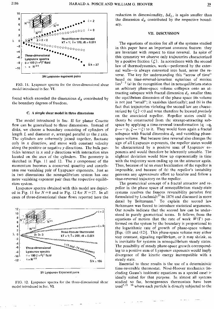
FIG 11 Lyapunov spectra for the three-dimensional shear model introduced in Sec VI
found which exceeded the dimensions dB contributed by the boundary degrees of freedom
C A simple shear model in three dimensions
The model introduced in Sec II for planar Couette flow can be generalized to three dimensions Instead of disks we choose a boundary consisting of cylinders of length L and diameter cr arranged parallel to the z axis The cylinders are coherently joined together fluctuate only in x direction and move with constant velocity along the positive or negative y directions The bulk parshyticles interact in x and y directions with interaction sites located on the axes of the cylinders The geometry is sketched in Figs 11 and 12 The z component of the momentum becomes a conserved quantity and contribshyutes one vanishing pair of Lyapunov exponents Just as in two dimensions the nonequilibrium system has one more vanishing exponent pair than the respective equilibshyrium system
Lyapunov spectra obtained with this model are depictshyed in Fig 11 for N 8 and in Fig 12 for N =27 In all cases of three-dimensional shear flows reported here the
FIG 12 Lyapunov spectra for the three-dimensional shear model introduced in Sec VI
reduction in dimensionality tdL is again smaller than the dimension dB contributed by the respective boundshyary
VII DISCUSSION
The equations of motion for all of the systems studied in this paper have an important common feature they are invariant with respect to time reversal In spite of this symmetry we observe only trajectories characterized by a positive friction lts) In accordance with the second law of thermodynamics work-performed by the extershynal walls-is always converted into heat never the reshyverse The key for understanding this arrow of time based on time-reversal-invariant equations of motion lies2- S (a) in the recognition that in nonequilibrium states an arbitrary phase-space volume collapses onto an atshytracting subspace with fractal dimension dL smaller than the equilibrium dimension of the phase space (its volume is not just small it vanishes identically) and (b) in the fact that trajectories violating the second law are characshyterized by lts) lt0 and must therefore be located precisely on the associated repellor Repellor states could in theory be constructed from the strange-attracting subshyspace by applying a time-reversal transformation (q---q p --- - p s--- - s) to it They would form again a fractal subspace with fractal dimension dL and vanishing phaseshyspace volume But because time reversal also changes the sign of all Lyapunov exponents the repellor states would be characterized by a positive sum of Lyapunov exshyponents and would therefore be inherently unstable The slightest deviation would blow up exponentially in time with the trajectory soon ending up on the attractor again Thus because of (a) an exact localization of the repellor is impossible and because of (b) the repellors instability prevents any approximate effort to localize and follow a time-reversed trajectory on the repellor
The geometrical concept of a fractal attractor and reshypellor in the phase space of nonequilibrium steady-state systems resolves the famous reversibility paradox first formulated by Loschmidt20 in 1876 and discussed in more detail by Boltzmann l To explain the second law Boltzmann was forced to introduce statistical arguments Our results indicate that the second law can be undershystood in purely geometrical terms It follows from the equations of motion that the rate of work W( r) pershyformed on the system by the boundary is proportional to the logarithmic rate of growth of phase-space volume [Eqs (to) and (12)] This phase-space volume may either stay constant signaling equilibrium or it may shrink as is inevitable for systems in non equilibrium steady states The possibility of steady phase-space growth correspondshying to a positive sum of Lyapunov exponents would imply divergence of the kinetic energy incompatible with a steady state
Essential to these results is the use of a deterministic time-reversible thermostat Nose-Hoover mechanics (inshycluding Gausss isokinetic equations as a special case) if ideally suited for that purpose In almost all systems studied so far homogeneous thermostats have been used522-26 where each particle is directly subjected to the
39 EQUILIBRIUM AND NONEQUILIBRIUM L Y APUNOV SPECTRA 2187
thermostatting constraint force In this paper however we study composite boundary-bulk-boundary nonequilishybrium systems in which only the boundary particles are thermostatted and are exposed to an external perturbing force The bulk region is composed of particles obeying solely Newtons equations In addition to all the irrevershysible properties summarized above we find an important new feature The reduction of phase-space dimension asshysociated with the irreversible flux can only with great difficulty exceed the dimension dB necessary to describe the state of the boundary This important result has been found previously in a study of heat flow from a hot to a cold reservoir4 but our shear-flow results presented in this paper make this conclusion much more convincing For small systems it seems to be difficult to reduce the dimensionality of the attracting subspace for the total system below a limit set by the dimension of the Newtonian bulk particles Only in one of the systems studied here does the reduction in dimensionality exceed dB In contrast to heat conduction4 the thermostatted boundary strongly influences the attainable phase-space dimensionality loss t1dL for the shear flow problems studshyied here
A new and important role has to be attributed to the few most negative Lyapunov exponents We have demonstrated in Secs V and VI that they have a decisive influence both on the sum of all Lyapunov exponents and the dimensionality loss The most strongly converging directions in phase space therefore largely determine the irreversible behavior This is in accord with the information-theoretical arguments by Shaw46 We have recently shown47 how the most negative Lyapunov exshyponents can be calculated without the need to compute the whole spectrum of exponents as required by the classhysical algorithms This method also provides the possibilishyty of obtaining negative exponents directly from experishymental time series
Shear flow in two and three dimensions can also be studied by continuum hydrodynamics48 Taking the Navier-Stokes equations as a starting point the Lyapunov spectra for planar shear flow at low49 and high5obull51 Reyshynolds numbers have been approximated by simulation Since the dimension of the state space of a partial differential equation is infinite the problem is numericalshyly approached by introducing a grid of points in phase space (100 X 100 are typical) and using finite-difference methods or Fourier techniques The dimensionality of the resulting caricature problem is then determined by the number of variables used in the simulation
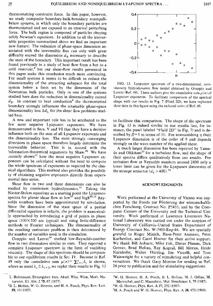
Grappin and Leorat49 studied low-Reynolds-number flow in two dimensions similar to ours They reported a complete Lyapunov spectrum in the limit of vanishing viscosity The shape ofthis spectrum should be comparashyble to our equilibrium results in Sec IV Because in Ref 49 only the cumulative sum fL( n) =If Ai is shown where as usual Ai ~ Ai +l we replot their results in Fig 13
04 I I o
o 0 0
0
02 I- 0 shy0
0 0
0 0 0
0 0 0 1-0 0 shy
0 0
0 0 0
00
- 02 I- shy
o o o
o -Q4~______J~______~1___~~~
n
FIG 13 Lyapunov spectrum of a two-dimensional zeroshyviscosity hydrodynamic flow model obtained by Grappin and Leorat (Ref 49) These authors give the cumulative sum -l(n) of Lyapunov exponents To facilitate comparison of the spectral shape with our results in Fig 7 (Fluid 2D) we have replotted their data in this figure using the reduced units of Ref 49
to facilitate this comparison The shape of the spectrum in Fig 13 is indeed similar to our results (see for inshystance the panel labeled Fluid 2D in Fig 7) and is deshyscribed by 1 in terms of (1) For non vanishing TJ their Lyapunov dimension is of the order of 9 and depends strongly on the wave number of the applied shear
A much larger dimension has been reported by Yamashyda and Ohkitani5o for a turbulent flow and the shape of their spectra differs qualitatively from our results For turbulent flow at Reynolds numbers around 2800 only a lower limit can be given for the Lyapunov dimension of the strange attractor (dL gt 400)51
ACKNOWLEDGMENTS
Work performed at the University of Vienna was supshyported by the Fonds zur Forderung der wissenschaftlishychen Forschung Contract No P5455 and by the Comshyputer Centers of the University and the Technical Unishyversity Work performed at Lawrence Livermore Nashytional Laboratory was carried out under the auspices of University of California-United States Department of Energy Contract No W-7405-Eng-48 We are specially grateful to Roger Minich Hans-Peter Axmann Peter Karlsreiter and Carol Hoover for their active support We thank Bill Ashurst Mike Feit Dieter Flamm Dick Grover Brad Holian Ray Kapral Bill Moran Heide Narnhofer Walter Thirring Jim Viecelli and Tom Wainwright for a variety of stimulating and helpful conshyversations We thank Gary Morriss for sending us Ref 24 prior to publication and for stimulating suggestions
L Boltzmann Sitzungsber kais Akad Wiss Wien Math Nashy 3W G Hoover H A Posch B L Holian M J Gillan M turwiss Kl Abt 27567 (1877) Mareschal and C Massobrio Mol Simulation 1 79 (1987)
2B L Holian W G Hoover and H A Posch Phys Rev Lett 4W G Hoover Phys Rev A 37 252 (1987) 59 10 (1987) 5H A Posch and W G Hoover Phys Rev A 38473(988)
2188 HARALD A POSCH AND WILLIAM G HOOVER
6W G Hoover Molecular Dynamics Vol 258 of Lecture Notes in Physics edited by H Araki J Ehlers K Hepp R Kipshypenhahn H A Weidenmiiller and J Zittartz (SpringershyVerlag Berlin 1986)
7J Ford Phys Today 36 (4) 40 (1983) 8S Smale Bull Am Math Soc 73247 (1967) 91 B Schwartz Phys Rev Lett 601359 (1988) lOS D Stoddard and J Ford Phys Rev A 81504 (1973) 11s Nose MoL Phys 52 255 (1984) uS Nose J Chern Phys 81 511 (1984) 13s Nose Mol Phys 57187 (1986) 14W G Hoover Phys Rev A 31 1695 (1985) ISD J Evans and B L Holian J Chern Phys 83 4069 (1985) 16W G Hoover A J C Ladd and B Moran Phys Rev Lett
481818 (1982) 17D J Evans J Chern Phys 783297 (1983) 18D J Evans W G Hoover B H Failor B Moran and A J
C Ladd Phys Rev A 28 1016 (1983) 19D J Evans in Molecular-Dynamics Simulation of Scatisticalshy
Mechanical Systems Proceedings of the International School of Physics Enrico Fermi Course XCVII Varenna 1985 edited by G Ciccotti and W G Hoover (North-Holland Amsterdam 1986)
20J Loschmidt Sitzungsber kais Akad Wiss Wien Math Nashyturwiss Kl Abt 2 73 128 (1876)
21B Moran W G Hoover and S Bestiale J Stat Phys 48 709 (1987)
22G P Morriss Phys Lett A 122 236 (1987) 23G P Morriss Phys Rev A 37 2118 (1988) 24G P Morriss (unpublished) 25W G Hoover H A Posch and S Bestiale J Chern Phys
876665 (1987) 26W G Hoover and H A Posch Phys Lett A 123 227 (1987) 27W T Ashurst PhD dissertation University of California at
Davis-Livermore 1974 28G Benettin L Galgani A Giorgilli and J M Strelcyn C R
Acad Sci SeI A 286 431 (1978) 29G Benettin L Galgani A Giorgilli and J M Strelcyn Mecshy
eaniea 15 9 (1980) 301 Shimada and T Nagashima Prog Thear Phys 61 1605
(1979) 3IJ_p Eckmann and D Ruelle Rev Mod Phys 57 1115-shy
(1985) 32A Wolf J B Swift H L Swinney and J A Vastano Physishy
caD 16 285 (1985) 33D J Evans Phys Rev A 32 2923 (1985l 34B L Holian Phys Rev A 344238 (1986) 35D J Evans and G P Morriss Phys Rev Lett 56 2172
(1986) 36W G Hoover W T Ashurst and R J Olness J Chern
Phys 60 4043 (1974) 37A J C Ladd B Moran and W G Hoover Phys Rev B 34
5058 (1986) 38R Livi A Politi and S Ruffo J Phys A 19 2033 (1986) 39R Livi A Politi S Ruffo and A Vulpiani J Stat Phys 46
147 (1987) 4oD M Heyes G P Morriss and D J Evans J Chern Phys
834760 (1985) 41J J Erpenbeck Phys Rev Lett 521333 (1984) 42H A Posch and W G Hoover (unpublished) 43B L Holian and D J Evans J Chern Phys 78 5147 (1983) 44B L Holian Phys Rev Lett 60 1355 (1988) 45J Kaplan and J Yorke in Functional Differential Equations
and the Approximation of Fixed Points Vol 730 of Lecture Notes in Mathematics edited by H O and H O Walther (Springer-Verlag Berlin 1980)
46R Shaw Z Naturforsch 36a 80 (1981) 47W G Hoover C G Tull and H A Posch Phys Lett A
131 211 (1988) 48p Constantin C Foias O P Manley and R Temann J
Fluid Mech150 427 (1985) 49R Grappin and J Leorat Phys Rev Lett 59 1100 (1987) 50~1 Yamada and K Ohkitani PhysRev Lett 60 983 (1988) 51L Keefe P Moin andJ Kim Bull Am Phys Soc 32 2026
(1987)
p1
p2
p3
p4
p5
p6
p7
p8
p9
p10
p11
p12
p13
p14
2176 HARALD A POSCH AND WILLIAMG HOOVER 39
t t
t t
Peano Smale
FIG 1 The Peano space-filling curve and the Smale horseshoe
7 the shape of Lyapunov spectra is typically simple For either two-dimensional or three-dimensional fluids and solids the equilibrium Lyapunov spectra can be crudely approximated by power laws
where n indexes the n max pairs of exponents and also represents the number of chaotic degrees of freedom For three-dimensional fluids 3 is approximately t for solids approximately I In two dimensions the correshysponding 3 values are 1 and f Because the Lyapunov spectra depend upon the trajectory bifurcations resulting from particle-particle or phonon-phonon collisions the exponents tend to increase with collision rate For simple fluids the expected increase with temperature and density has been observed 510
(2) Away from equilibrium mass momentum and enershygy currents respond to gradients in concentration velocishyty or temperature Reversible nonequiIibrium systems incorporating such flows can be simulated by applying external velocity or temperature perturbations or by imshyposing an external field The dissipation associated with such mechanically reversible thermodynamically irrevershysible flows invariably produces heat as summarized by the second law of thermodynamics To achieve a steady state under such nonequilibrium conditions a thermosshytatting procedure must be introduced The thermostat is required to extract the heat energy fed into the system by
the external perturbation Many types of thermostats have been proposed and used in simulations Theoretishycally it is desirable that such a thermostat retain the reshyversible and deterministic character of the fundamental laws of motion This can be achieved by eithermiddot Nose-Hooverll- 15 or Gaussian15
-19 reversible thermosshy
tats The Nose-Hoover thermostats have an aesthetic adshyvantage in that at equilibrium they generate Gibbss canonical phase-space distribution Either type of thershymostat is described by time-reversal-invariant equations of motion a reflection of the Hamiltonian basis they share as emphasized by Nose But neither of these revershysible thermostatted sets of motion equations is Hamilshytonian
(3) Lyapunov spectra are insensitive to ensemble both at and away from equilibrium At equilibrium completeshyly isolated (microcanonicaD systems have spectra very similar to those of thermostatted (canonical or isokinetic) systems The precise nature of the thermostatting mechshyanism is immaterial Our present nonequilibrium results likewise indicate that a similar insensitivity prevails in nonequilibrium systems Thus both at and away from equilibrium the irreversible chaotic motion of N-body systems is insensitive to the choice of statistical ensemble On the other hand boundary effects do influence the shape of the spectrum for small systems Thus periodic systems have simpler Lyapunov spectra than do systems confined by rigid walls
(4) For steady-state nonequilibrium systems the symshymetry of the Smale pairs of Lyapunov exponents is broshyken The sum of each pair of exponents shifts to a negashytive value corresponding to a loss of phase-space volume This means that the phase-space probability density colshylapses onto a strange attractor a fractal subspace with zero phase-space volume and with a Kaplan-Yorke fracshytal dimension significantly smaller than the dimension of the full phase space In the most extensively studied case field-driven charge conductivity for a dense fluidS the low-field reduction in phase-space dimension varies as the square of the applied external field This appearance of a phase-space strange attractor provides a simple and natushyral explanation for the irreversible behavior of such sysshytems in accord with the second law of thermodynamshy
5ics2 - For these reversible nonequilibrium systems Loschmidts reversibility paradox2o has thereby been resolved
The irreversible collapse of the phase-space density onto a strange attractor was first observed in few-body systems described by three-dimensional phase spaces with only three Lyapunov exponents These investigations inshycluded simulations of a periodic two-dimensional isokishynetic Lorentz gas or Galton board driven by an external field1 of a one-body one-dimensional FrenkelshyKontorova model for isothermal electronic conduction3
22 24and of an isokinetic two-body planar shear flOW shy
Further work included the simulation of complete Lyapunov spectra for systems of up to 32 particles in three dimensions under both equilibrium25 and nonequilishybrium26
bull5 conditions In most of the nonequilibrium
work a homogeneous thermostat has been used with each particle of the system under study subjected to the
2177 EQUILIBRIUM AND NONEQUILIBRIUM L Y APUNOV SPECTRA
thermostatting constraint force Both Nose-Hoover thershymostats characterized by a response time I and Gaussshyian thermostats corresponding to the limit have been employed
Closer to experiment and therefore of more inshyterest are the boundary-bulk-boundary nonequilibrium systems as indicated schematically in Fig 2 and investishygated earlier2724 Such systems may incorporate two or more boundary regions in which particles interact with an external force and a thermostat with a bulk region sandwiched between the boundaries In the bulk Newtonian regions the particle motion is solely governed by Newtons equations of motion In the heat-flow case with the geometry illustrated in Fig 3 the boundary reshygions on the left and right represent hot and cold resershyvoirs The heat transported through the Newtonian bulk system can then be studied4
In this paper we present the results of extensive simulashytions of two-dimensional shear flow (plane Couette flow) for systems of N two- or three-dimensional bulk Newtonian particles A typical situation is sketched in Fig 3 The bulk particles are enclosed by a downmoving vertical boundary to the left and an upmoving vertical boundary on the right with periodic boundaries linking the top and bottom of the system By fixing the normal separation of the two moving boundaries to a constant value it is possible to describe their horizontal (x) motion with a single degree of freedom thermostatted by a single Nose-Hoover thermostat This model evolved so as to minimize the boundary and thermostat degrees of freeshydom and is described in more detail in the following secshytion A modified two-dimensional shear model with two boundary degrees of freedom is discussed in Sec VI A Extensions to shear flow in three dimensions are treated in Sec VI C
The method for determining the model Lyapunov specshytra is discussed in Sec II Our simulation results for sysshytems involving up to N 81 bulk particles in two dimenshysions and N =27 particles in three dimensions are all reshyported in Secs III-VI As detailed in Secs IV and VI
Cold
FIG 2 Schematic illustration of a boundary-driven noneshyquilibrium steady-state heat-flow simulation The system is dishyvided into three communicating chambers by vertical walls Periodic boundaries link the top and bottom boundaries Partishycles in the left- (right-) hand region are maintained at a hot (cold) temperature by Nose-Hoover or Gaussian thermostats Particles in the Newtonian bulk region transmit heat on the average from the hot to the cold region
kT=1 y= -5
kT=1 y= +5
FIG 3 Snapshot showing a typical 16-particle configuration during a nonequilibrium shear-flow simulation with a strain rate 1=2 The boundary sites at the left (right) move down (up) ward at a speed (+) 5 Periodic boundary conditions link the top and bottom of the volume The thermal temperature of the boundary in the horizontal direction corresponds to kT = 1 as explained in the text This figure illustrates that the positive shear causes particle collisions to occur preferentially with negshyative values of XiJYij making a negative potential contribution to the xy component of the pressure tensor Here r ij = (x ijy ij )
stands for the vector separating two arbitrary Newtonian partishycles or a Newtonian particle and a boundary interaction site
these spectra have shapes qualitatively unlike those found earlier in three dimensions For two-dimensional fluids the l3 of Eq (1) of found in three dimensions is instead close to 1 This corresponds to the one-dimensional Debye model in which the density of k-space states is constant Further the presence of nonequilibrium condishytions strongly changes the spectrum The dependence of the Lyapunov spectrum on system size and strain rate is characterized Section VII contains a discussion of our results and a brief comparison with corresponding model results from continuum hydrodynamics
n BOUNDARY-DRIVEN ISOTHERMAL SHEAR FLOW
The geometry of a typical two-dimensional nonequilishybrium system is shown in Fig 3 The bulk Newtonian reshygion consists of N two-dimensional particles of mass m These interact with each other and with the boundary sites with a short-ranged purely repulsive potential
JlOOEo[ 1 - (r I a 2]4 if r lt a
lo if r a (2)
In what follows including the figures and tables we use reduced units The mass m as well as the potential pashyrameters EO and a are unity We introduced this potenshytial previously2526 to eliminate errors from discontinuishyties in low-order derivatives of cp at the cutoff distance r =a ( 1)
The Newtonian bulk region is bounded in the positive and negative x directions by vertical columns of equally spaced boundary interaction sites (shown as lightly shadshy
2178 HARALD A POSCH AND WILLIAM G HOOVER
ed in Fig 3) These boundary sites are arranged parallel to the vertical (y) axis The spacing between adjacent boundary sites (T (= 1) is equal to the potential cutoff distance There are L I (T interaction sites for each boundary L is the periodicity interval for the periodic boundary conditions applied in the vertical direction The horizontal (x) spacing between centers of the two columns of sites is kept constant and equal to L + (T In all simulations L was chosen to be equal to liN (T thus fixing the number density N IL2 of the Newtonian bulk particles at 1 All of the boundary sites are coherently joined together so that their horizontal momentum reacts to the summed interactions of all of the bulk partishycles which lie within unit distance of any boundary site The total mass associated with the x motion of the boundary sites is unity the same as the mass of a single Newtonian bulk particle The thermodynamic temperashyture associated with the boundary sites is also taken to be unity and is enforced by a Nose-Hoover thermostat which guarantees on a time-averaged basis that the flucshytuating part of the boundary kinetic energy P 12m has the equipartition value t
(3)
Here is the momentum in the x direction of all 2L boundary sites with a combined mass equal to the mass m 1 of a Newtonian particle ( gt denotes a time average k is Boltzmanns constant and T is the average temperature of this horizontal boundary degree of freeshydom No thermal fluctuations of the boundary motion in the vertical (y) direction are allowed In this direction the boundary particles move with a constant velocity VB related to the imposed strain rate eby
+(T)e (4)
where the plus and minus signs refer to the right- and left-hand columns of boundary sites respectively It is sufficient to solve the equations of motion for a single boundary site by properly adding all interactions linking bulk and boundary particles using appropriate periodic boundary conditions in the y direction We denote the position of this reference site by R = (X Y) and its flucshytuating momentum by P=(PxO) The positions of an arshybitrary boundary particle are given by RB = (XB YB ) If furthermore TnPn denote the respective positions and momenta of the bulk particles (n 12 N) then the equations of motion of our model system take the form
Til =Pn 1m
(5) (L+(T)e2
ix -altPintaX -tPx
~=(PlmkT-l)
Here ~N is the potential energy of the Newtonian bulk (assumed to be pairwise additive) and ltPint is the interacshy
tion energy between the Newtonian particles and the moving walls
ltPN= ~ ~ 1gt( irn-rlll) n ( fl) n
(6) ltPnt= ~ ~ 1gt( Irn-R B )
B n
The sum over B is over all 2L I (T interactions sites of the boundary
Extension of this model to three dimensions is straightshyforward Either spherical or cylindrical boundary partishycles can be used We have chosen cylinders to avoid inshyducing motion in the z direction This model is discussed in more detail in Sec VI C
The thermostat variable t which causes the boundary momentum to fluctuate on a timescale T in the x direcshytion is an independent variable arising as a momentum in Noses original derivation Thus in two (three) dimenshysions the dimensionality of the phase space is increased from the bulk-particle value of 4N (6N) to 4N +4 (6N +4) including the x coordinate and momentum of the boundary reference site its y coordinate and the fricshytion coefficient t The dimension of the phase space is of crucial importance in the description and discussion of the results of our simulations
Let the flow equations (5) be abbreviated by
(7)
where r (rnPnXPx Yt) is a (4N +4)-dimensional state vector In principle the 4N +4 Lyapunov exshyponents are calculated by solving-in addition to (7)-the 4N +4 linearized sets of equations28 - 32
(8)
where I 12 4N +4 for the two-dimensional case D(r)=aG(r)ar is a quadratic dynamical matrix which couples the reference trajectory to the differenshytially separated satellite trajectories represented by 8(t) An arbitrarily oriented set of orthonormal vectors can serve as initial condition for the vectors 8[ (t) In the course of time these vectors do not stay orthonormal but tend to rotate into the direction of maximum phase-space growth By application of a Gram-Schmidt orthonormalshyization procedure every few time steps one finds that the vector 81 tends to point uniquely into a direction of most rapid phase space growth [proportional to exp(j t)] Similarly 8182 span a subspace whose area grows most rapidly [proportional to exp( Ai + A)t] and so forth From this sequence all Ai are obtained The Lyapunov exponents are the time averages of these quantities
(9)
In practice we follow the trajectories forward for a time t of the order of 1000 employing a fourth-order Runge-Kutta integration scheme To avoid initial transhysients we exclude the first 30 of the trajectory from the averaging procedure For almost all simulation results we report in the following sections a reduced time step
39 EQUILIBRIUM AND NONEQUILIBRIUM L Y APUNOV SPECTRA 2179
At =0001 is used all exceptions being specially marked at the appropriate places
The sum over all Lyapunov exponents (~A) is equal to the averaged logarithmic rate of growth of the phaseshyspace volume In our case this means that
(10)
where as in (9) lt ) denotes a time average (in practice over the length l of the run) The quantity A =d alar) t(t) is called the phase-space compressibility The sum rule (10) provides a convenient test for the conshysistency of our simulation results Typically (10) is fulfilled to an accuracy of at least four significant digits
The internal energy of our boundary-bulk-boundary shear problem (5) is given by
Making use of the equations of motion the rate of change ofH(r) is given by
aH rmiddot = (12)ar where
(13)
The sum in the last equation is over all boundary interacshytion sites and YB is given by (4) Since altlgtintaYB is the total frictional force component parallel to the shear exshyerted by the boundary site B on the bulk W( r) is the rate of work performed on the system by the boundary The first term on the right-hand side of (12) is the rate at which heat is extracted by the thermostat In nonequilishybrium steady states both terms cancel each other (inn) =0 from which we find a quadratic strain-rate dependence of the averaged friction (s)
(14)
In this equation 7 is the viscosity defined by
(15)
The factor 2 accounts for the total length of the comshybined left and right boundaries Equation (14) is used to obtain 7J from the simulation results for (s)middot
Integrating (12) one finds that the quantity
(16)
is constant along a trajectory r(t) both at equilibrium (for which W vanishes) as well as in nonequilibrium states We have verified that HNose is indeed conserved by our simulations However the total momentum of the boundary-bulk-boundary system is not a constant of the motion 13 The consequences are discussed in Sec III
The information-theory entropy is defined by
Sinf=-k Jdr j(rt)lnj(rt) (17)
where j (r t) is the phase-space distribution function Equating time averages with ensemble averages over the non equilibrium ensemble one finds for the rate of change of Sinf (Refs 33 and 34)
(18)
For non equilibrium steady-state conditions the rate of change of Sinf is balanced by the rate of (global) irreversishyble entropy production
(19)
which according to (14) is a positive quadratic function of the applied strain rate t
The thermostat response time T enters the Nose equashytions of motion as a free parameter In what follows we require that T is proportional to the mean collision time between bulk particles and the boundary Because in two dimensions the respective collision rate is proportional to the periodicity interval in the y direction L we choose T= IlL (in our reduced units) In three dimensions T= 1L 2 The Lyapunov spectra reported in the followshying sections are insensitive to this choice Furthermore the boundary thermostat temperature T chosen for all our simulations corresponds to kT = 1
The linear differential equation for Yin (5) is associated with a vanishing Lyapunov exponent From a practical point of view it is advantageous to avoid the timeshyconsuming computation of this vanishing exponent in an ordered sequence Ai Ai + I as required by the algoshyrithms This can be achieved by replacing this trivial differential equation by its integral Y(t)= Vt + Y(O) and using Y(t) for the evaluation of ltlgtint This converts the autonomous system of flow equations (5) with (4N +4)dimensional phase space into a non autonomous system of order 4N + 3 and reduces the number of exshyponents to be calculated by one In three dimensions 4N is replaced by 6N
At relatively high strain rates the kinetic energy of some Newtonian particles might become large enough to overcome the potential barrier imposed by the walls In this case a Newtonian particle can escape by slipping beshytween two neighboring boundary interaction sites In our first runs we were alerted to this problem by noticing that pairs of Lyapunov exponents started to vanish two pairs for each escaped particle We then prevented such esshycapes by imposing an elastic reflection whenever a bulk particle attempted to cross the boundary lines x =X and x = X + L + a respectively
III MAXIMUM LYAPUNOV EXPONENTS
The maximum Lyapunov exponent Amax reflects the rate of the fastest dynamical events taking place in phase space In Table I this quantity is listed for the twoshydimensional simulations for various system sizes N both at equilibrium (t=O) as well as in nonequilibrium steady states Also given in this table is the time-averaged thershy
2180 HARALD A POSCH AND WILLIAM G HOOVER 39
TABLE I Parameters for two-dimensional equilibrium systems (t=o) with various system sizes N The particle density is 1 ltK) is the kinetic energy of thc Newtonian bulk particles and TN their temperature lt1raquo is the total potential energy (including boundary-bulk interactions) The mean kinetic energy of the boundary is 050 in accordance with a boundary temperature given by kT = 1 tis the duration of the run with a time step 0001 max is the maximum Lyapunov exponent and 11K is the Kolmogorov enshytropy the sum of the positive Lyapunov exponents is the Lyapullov dimension which-for mixing equilibrium systems-i~ equal to the number of variables necessary to uniquely define the microscopic system state The estimated uncertainty for Amax is plusmn06
N=4 N=9 N 25 =o
N=36 N=49 N=64 N=81 N 100
(K) lt1gt )
1 ~
x
hK
40 15 100
8000 273
19
90 42 100
1010 303
39
154 73 096
1600 316
31 67
253 119 101
2000 329
103
359 167 100
1100 335
137 147
506 233
103 1300
341
199
650 297
102 1300
347
259
812 375
100 2000
349
327
98 45
098 460
35
403
mostat friction coefficient (s) and the peculiar kinetic energy per bulk particle defined by
(20)
p(Tn )=mpound[xn - X -L +cr )2]51 is the momentum at the position of particle n corresponding to a linear velocishyty profile between the moving boundaries where y is the unit vector in the y direction K 11 is equal to the peculiar temperature of the Newtonian bulk It should be kept in mind however that this definition is based on the assumption of a linear velocity profile which is not necessarily correct 35 In general l can differ from the thermostat temperature T for nonequilibrium conditions
Consulting Fig 4 one finds that )max increases logarithshymically with system size 11 both at equilibrium as well as in non equilibrium steady states This result also persists if the free volume due to the roughness of the boundshyary is taken into account which reduces the density by 4 for 11 =4 and by 2 for 11 16 These corrections
12 CI
Amax CI
E CI2
o E=18 CI
A CI
4
3 5InN
FIG 4 The maximum Lyapunov exponent Amax as a function of the logarithm of the system size for equilibrium systems (t=O crosses) and nonequilibrium steady states (1=1 squares =2 triangles)
for the density5 are too small to affect the logarithmic dependence of Amax with 11
For equilibrium systems (pound=0) a logarithmic systemshysize dependence of Ama is not totally unexpected It is well known that there is a formal analogy between the viscous stress due to velocity gradients in incompressible fluids and elastic stress due to displacement gradients in harmonic solids36 The fastest mechanism which detershymines Amax for a crystal is phonon-phonon scattering37
The cross section for this phonon-phonon interaction is proportional to the mean-squared displacement of a typishycal particle from its lattice site It has been shown by lattice-dynamical simulations of small two-dimensional crystals composed of N particles36 that the mean-squared displacement increases as InN The proportionality coefficient agrees exactly with that estimated from conshytinuum elastic theory By invoking this analogy between elastic and viscous stress a logarithmic dependence of Amax on the system size could be expected also for a twoshydimensional fluid This is consistent with our simulashytions
It is interesting to note that Stoddard and Ford1O in their pioneering numerical study of the mixing behavior of dilute Lennard-Jones gases estimate a logarithmic dependence of Amax on system size for planar systems Their arguments are based on a crude kinetic theory of hard disks
The relation between Amax for a fluid and the meanshysquare displacement of an appropriate solid should also hold in three dimensions We have previously shown5
that Amax for a three-dimensional fluid system does not depend on the system size This is in agreement with the constant limiting value for the mean-squared displaceshyment of a related solid in three dimensions In one dishymension there appears to be much less number depenshydence 38 39
For nonequilibrium steady-state conditions (with fixed strain rate tgt 0) the relative kinetic energy per particle K 11 does not stay constant if the system size is inshycreased As a consequence the slope of the graphs of
versus InN increases with pound as depicted in Fig 4
2181 EQUILIBRIUM AND NONEQUILIBRIUM L Y APUNOV SPECTRA
An interesting but unexpected phenomenon takes place for larger strainrates (t 2) and large enough systems (N gt 36) It has been mentioned already in Sec II that the equations of motion (5) do not conserve the total momentum of the boundary-bulk-boundary system
d -~Px (21)
dt [~Pn +P] = - ~ altlgtintaYn n J
The nonvanishing x component causes a slow drift of the whole system along the x axis without affecting the reshysults Because of the non conserved Y component of the momentum it is possible however that the Newtonian bulk may lose coupling with a system boundary and start moving with an average velocity equal to that of the left or right boundary This consequence resembles an order-disorder transition and the maximum Lyapunov exponent quickly drops far below its expected steadyshystate value Figure Sea) shows the time evolution of f1A( tldt It as a function of the duration of the run t for
OL-_-~~L_~~~~_~---~
o 500 1000 1500
FIG 5 (al Curve A shows the convergence of the maximum Lyapunov exponent for a 49-bulk-particle system sheared at a shear rate pound=2 1 is the run time The same system with different initial conditions suffers a transition into a more orshydered state at 1 around 400 which leads to a fast decrease of the maximum Lyapunov exponent as exemplified by curve B (bl Snapshot of the particle configuration at a run time 1= 1500 of curve B in (a) The bars indicate the direction and magnitude of the instantaneous particle velocities The left (right) boundary moves down (up) with a velocity equal to 8 in reduced units The particle diameter is a 1
two simulations of a 49-partic1e system starting from different initial conditions One of these trajectories exshyhibits this sudden transition in the time interval covered by the simulation An instantaneous snapshot of the fluid structure of such a partially decoupled bulk phase movshying along with the right-hand boundary in the positive Y direction is shown in Fig S(b)
Other kinds of order-disorder transitions have been obshyserved recently in nonequilibrium molecular-dynamics simulations of shear flow both in tw040 and three41 dishymensions In these simulations momentum-conserving homogeneous thermostats were used It has been found that for larger shear rates the particles are preferentially arranged along stream lines giving rise to a significant deshycrease of the viscosity (shear thinning)
IV LYAPUNOV SPECTRA FOR TWO-DIMENSIONAL EQUILIBRIUM SYSTEMS
Systems in equilibrium which evolve according to time-reversible equations of motion have symmetric Lyapunov spectra for each positive exponent there is a corresponding negative one with equal absolute magnishytude The sum over all exponents vanishes indicating conservation of phase-space volume For such a system it is therefore sufficient to plot only the positive branch of the spectrum the negative being a mirror image with respect to the abscissa As an example we show in Fig 6 the spectrum of a 36-partic1e system at equilibrium (pound=0) Including the boundary and the friction ~ which vanishes on the average there are 4N +3 147 exshyponents altogether of which three exponents vanish All 72 exponents greater than zero are shown in Fig 6 The abscissa can be thought of as labeling the various exshy
FIG 6 Lyapunov spectrum for a 36-bulk-partic1e system in equilibrium (pound=0) The boundary Nose-Hoover thermostat acts in the horizontal x direction and has only one degree of freedom (g I) The thermostat response time is 1= i The time step used for the simulation is equal to 0001 There are alshytogether 4N +3= 147 Lyapunov exponents of which 72 exshyponents greater than zero are shown in the figure The negative branch of the spectrum is a mirror image around the abscissa and is not shown Four vanishing exponents are suppressed The abscissa indexes the exponents and is not specially labeled
2182 HARALD A POSCH AND WILLIAM G HOOVER 39
ponents by a Lyapunov index n with n = I for the smallshyest positive exponent and n =72 for the top-right maxshyimum exponent Amax The index n (A) can be interpreted as the number of positive exponents less or equal to A Parameters related to this spectrum are also contained in Table I
This spectrum is relatively simple But there is no theoretically founded expression describing the shape of the spectrum in Fig 6 In terms of the empirical formula (1) a linear relation (3= 1) seems roughly appropriate It is interesting to note that there is a qualitative difference between the shapes of the Lyapunov spectra for fluids and solids both in two (2D) and three (3D) dimensions The details are shown in Fig 7
A Fluid 2D
This spectrum corresponds to a nine-particle fluid in two dimensions thermostatted as described in Sec II and interacting via the potential (2) Relevant parameters are listed in Table I There are 18 positive exponents in this case
B Solid 2D
This spectrum corresponds to an isoenergetic microshycanonical two-dimensional hexagonal solid composed of 12 particles in a cell with periodic boundaries again inshyteracting with the purely repulsive potential (2) The nearest-neighbor separation is 09 reduced units correshysponding to a reduced particle density of 1426 The poshytential and kinetic energies assume the values 108 and 59 respectively and the reduced temperature is 049 The sum of all positive Lyapunov exponents determines the Kolmogorov entropy and is equal to 806 in our reshyduced units of Sec II There are 4N =48 Lyapunov exshyponents of which eight vanish Twenty exponents greater
n n 44
Fluid 2D )) 0dega 0 0
0 0
0 02 20
0 0
0 a a
0 0
o a 0 10 10
Solid 2D )(
05 05
0 0 n n
FIG 7 Comparison of Lyapunov spectral shapes for solids and fluids in equilibrium The label 2D or 3D indicates whether the system is two or three dimensional All further information is given in Sec IV of the main text As in Fig 6 only the posishytive branches of the spectra are shown The abscisse merely inshydex the exponents and are not labeled
than zero are shown in the figure The smooth curve is a fit of (1) to these points yielding 3= 1 6
C Fluid 3D
This is a Lyapunov spectrum for an eight-particle three-dimensional fluid in isoenergetic equilibrium 5 The particles interact via a repulsive Lennard-Jones potential and the Lyapunov exponents are given in Lennard-Jones reduced units Relevant parameters are listed in Table I of Ref 5 (state I) The smooth curve is a fit of (1) to 20 points greater than zero giving -5
D Solid 3D
This spectrum is for a 32-particle fcc solid in three dishymensions and isoenergetic equilibrium42 Periodic boundshyary conditions are employed The particles interact via a Lennard-Jones (LJ) potential with LJ parameters ELJ and aLJ The potential is smoothly truncated at V3aLJ by fitting a cubic spline at the inflection point (yen )1I6aLJ
This potential has been used also by Holian and coshyworkers in their study of fluid viscosity43 and fragmentashytion44 by molecular dynamics All quantities related to this spectrum are given in LJ-reduced units The number density is 10 and the time-averaged potential and kinetic energies are 1750 and 263 respectively This correshysponds to a reduced temperature kT =0 55 The Kolmoshygorov entropy becomes 468 There are 6N - 10 nonvanshyishing exponents and 91 exponents greater than zero are plotted in the figure The data are represented quite well by a straight line corresponding to 3= I in terms of Eq (1)
Inspection of the data displayed in Fig 7 reveals significant qualitative differences in the shape of the specshytra for fluids and solids both in two and three dimensions A fundamental understanding of these results is still missshying It is hoped that at least for solids an interpretation of the spectra in terms of lattice-dynamical concepts will be obtained soon
V LYAPUNOV SPECTRA FOR TWOmiddotDIMENSIONAL SYSTEMS IN NONEQUILIBRIUM STEADY STATES
By steadily shearing the planar systems introduced in Sec II the symmetry of the Lyapunov spectra is lost The rate of global entropy production equal to the timeshyaveraged thermostat variable (() and according to (9) the negative sum of all Lyapunov exponents must be posshyitive for nonvanishing t In Fig 8 we show Lyapunov spectra for different system sizes for a shear rate t= 1 Analogous spectra for t = 2 are depicted in Fig 9 The abscissa is given by the Lyapunov index n and has not been labeled in these figures to permit a clear presentashytion Only non-negative exponents are plotted Further relevant information for these runs is collected in Tables II and III This includes the viscosity calculated from (14) the Reynolds number
N =mNf2(L+a)2t 3
(22)Re L2 kT()
39 EQUILIBRIUM AND NONEQUILIBRIUM LY APUNOV SPECTRA 2183
Two-dimensional Sik =(I ) = - L A= Lyapunov spectra 113673010 p = 100 1_r2)4 fluid Nose-Hoover thermostat
kT= 1 E= 2 1=1000 dt 0001
2N + 1 Lyapunov exponent pairs
FIG 8 Two-dimensional Lyapunov spectra for a shear rate t = 1 and various system sizes as indicated by the label (N = LX L in reduced units) The boundary thermostat has a single degree of freedom (in the x direction) as outlined in Sec II The relevant parameters for these spectra are collected in Table II Vanishing exponents are not shown dt is the time step for the simulation and tis the length of the run All paramshyeters are explained further in the text and are given in reduced units The abscissa merely indexes the exponents and is not lashybeled
and the fractal dimension dL of phase space discussed below
When increases the shape of the spectrum changes in a very pronounced way the slopes of both the positive and negative branches increase in absolute value In adshydition the spectrum is shifted downward The most posishytive exponents are increased noticeably But the most
TABLE II Parameters for the two-dimensional system sheared at a rate E= L N is the system size K is the relative kinetic energy of the bulk particles defined in (20) lt~ gt is the time-averaged Nose friction coefficient 7J the viscosity defined in (14) and N Re is the Reynolds number estimated from (22) The mean kinetic energy of the boundary is 050 in agreement with the boundary temperashyture given by kT = 1 The density of the bulk mNIL 2= 1 tdL is the loss in phase-space dimensionality as explained in Sec V The other parameters are defined in Table I All quantities are given in reduced units The four most negative Lyapunov exponents the
and
N=4
(KIN 18 ltltP gt 30 t 8000 max 329
The four most -23 negative -26 Lyapunov -30 exponents -34
hK-lt0
15 284
N Re 13
7J 048 08
2N + 1 Lyapunov exponent pairs
FIG 9 Two-dimensional Lyapunov spectra for a shear rate I = 2 and various system sizes as indicated by the label (N = L XL in reduced units) The boundary thermostat has a single degree of freedom (in the x direction) as explained in Sec II Relevant parameters for these spectra are given in Table III Vanishing exponents are not plotted For the larger systems some of the most negative exponents are far off the scale of this figure and are not shown but listed in Table Ill As usual the abscissa merely indexes the exponents and is not specially lashybeled
dramatic change takes place with the most negative exshyponents which become so negative that they do not fit on the scale of Fig 9 The four most negative exponents are listed in Tables II and III along with max for some of the spectra studied
The asymmetry of the Lyapunov spectra in the noneshyquilibrium case implies that the sum of all Lyapunov ex-
are taken from a different run illustrated in 8
t=1 N=9 N=16 N=25 N=36
~~---~------~-----
25 41 63 106 310 74 148
2020 2760 1340 1100 428 552 678 795
-36 -53 -64 -41 -56 -67 -44 -59 -87 -46 -63 -9
40 84 147 863 187 316 464
17 22 29 38 072 094 105 110 19 32 4
N=49 N=64 N=81
148 175 261 436 642 104 1260 1480
895 993 108
620 853 114 51 61 71
111 118 126
2184 HARALD A POSCH AND WILLIAM G HOOVER 39
TABLE III Parameters for two-dimensional systems sheared at a rate E = 2 All the quantities are defined in Tables I and II and are given in reduced units The four most negative Lyapunov exponents the Kolmogorov entropy hK and the phase-space reduction 1dL are taken from a different (shorter) run illustrated in Fig 9
ponents which according to (10) is equal to the averaged phase-space compressibility ltA) is always negative This means that an arbitrary hypervolume in phase space shrinks in the course of time and develops into a very complicated fractal-like subspace The dimension of this fractal object dL can be obtained from the number of exshyponents needed for the cumulative sum f1(J)= Lf=l Ai (with Ai 2 Ai +1) to change sign According to the Kaplan and Y orke45 linear interpolation formula one has
_ f1(J) (23)dL -J +-IA--I
J+l
where the integer J is obtained from the conditions f1(J) 2 degand f1(J + 1) lt 0
In Tables II and III we also list the reduction in dimenshysionality J1dv of the accessible phase-space volume from its equilibrium value caused by the dissipative perturbashytion pound0 This number is obtained from J1dL
=dL(O)+ I-dL(pound) where dL(O) is taken from Table I and the addition of 1 accounts for the Y coordinate of the boundary (which in equilibrium is a constant for this model) One immediately notices that J1dL never exceeds dB =4 the dimension contributed by the boundary deshygrees of freedom XPx Ys This is an interesting and significant result It means that an increase of the shear rate will result-according to (4) and (15)-in an inshycrease of lts) and consequently of 7] but the shape of the Lyapunov spectrum changes sufficiently to keep the loss in dimensionality below dB This is possible only by still further reducing mainly the last few most negative exshyponents to produce the necessary reduction in the sum of all exponents This is precisely what is generally obshyserved It should be noted in this context that the conshysiderations in Ref 4 do not apply to the boundary-bulkshyboundary problems treated here because of this strange behavior of the most negative exponents We expect that this shape change would be much less severe if more
boundary degrees of freedom were present To test whether this result is of a general nature we
simulated further shear models both in two and three dishymensions which differed in the dimension dB needed to describe the action of the boundary These results follow in Sec VI
VI MODIFIED SHEAR MODELS IN TWO AND THREE DIMENSIONS
A Planar Couette flow with a modified Nose thermostat
We increase the dimension dB contributed by the boundary thermostat by allowing the boundary interacshytion sites to fluctuate thermally not only in the x direcshytion (as in Sec IV but also in the y direction the direction of the shear There are two thermostatting degrees of freedom g = 2 as compared to one for the model of Sec II The equations of motion now assume the form
Pn = -a(ltPN+ltPint)arn
R=Plm -f(L +a)poundy (24)
p= -altIgtint aR -sP t=(p2I2mkT-l)h2
As before R = (X Y) denotes the position and P =(Px Py ) the thermally fluctuating part of the momenshytum for the boundary reference site y is the unit vector in y direction The thermostat temperature is now detershymined by
kT=(P+P)2m (25)
instead of (3) and the sum rule 00) takes the form
2185 AND NONEQUILIBRIUM L Y APUNOV SPECTRA
(26)
where A is the sum over all exponents In practice this equation for a 16-particle system is obeyed with a precision- of at least five significant figures after 300000 time steps
Similar to (16) the quantity
P~ p2 HNose(rJ=ltlgtN+ltlgtint + 2 2 + 2 +
m m
- ftW(rJdt+gkT ffdt (27) o 0
(g =2) is a constant along the trajectory r(t) where W by (13) is the rate at which work is performed on
the system by the boundary The value of depends on the choice of the time origin We have verified that (27) is conserved by our simulations As in the shear model of Sec II the total momentum is not a constant of the motion
4N +5 variables are needed to characterize uniquely the state vector r = (rn Pn R P () of the system Conseshyquently the equilibrium phase-space dimension dL (0)
4N +5 The reduction in phase-space dimensionality due to the dissipative perturbation is given by tdL =4N +5-dL (pound) The dimension contributed by the boundary degrees of freedom is dB = 5
Figure 10 shows results of such simulations for systems consisting of N =4 and N = 16 Newtonian bulk particles and a boundary shear rate t = 2 Relevant parameters are given in Table IV The shapes of the sheared-fluid specshy
~
tra are very similar to that for corresponding curves in
Index n
FIG 10 Full Lyapunov spectra for the modified twoshydimensional shear system introduced in Sec VI under noneshyquilibrium steady-state conditions pound=2 In contrast to Figs 8 and 9 the boundary Nose-Hoover thermostat has two degrees of freedom (g =2) The systems studied have four and 16 bulk particles respectively Further relevant parameters are given in Table IV There are altogether 21 and 69 Lyapunov exponents
~in these cases respectively of which two vanishing exponents Ire not shown in the although they have to be counted in the evaluation of the dimensionality Some of the most negative exponents do not fit on the scale and are listed in Table IV inmiddotmiddot stead
TABLE IV Results for the modified shear model of Sec VI A The boundary thermostat has two fluctuating of freedom (g 2) All quantities are defined in Tables I and II
in reduced units and 2 f is the sum over all
pound=2 N=4 N 16
(K)IN 41 127 ( ltlgt ) 63 796 t 2000 1500
Amax 438 785
The five -312 -803 most 372 -874 negative -440 -1104 Lyapunov 509 -1417 exponents 665 3346
hK 182 106 2 I 1303 -7611 (sgt 652 3806 NRe 42 84
027 048lJ 261 509plusmn0015
Fig 9 Of particular interest is the reduction in phaseshyspace dimensionality obtained for N 16 The equilibrishyum phase-space dimension dL (0 69 Application of a shear with a shear rate t=2 reduces this number bv tdL = 5 09plusmn0 015 The phase space contracts towards ~ fractal subspace with a dimension dL = 63 91 a number slightly but significantly smaller than the dimension 4N =64 contributed by the Newtonian bulk particles The standard deviation for adL was estimated by dividshying the trajectory into batches of 100 time units each This example shows that-by perturbing a system with an external boundary-it seems to be possible to obtain a reduction in dimensionality larger than the dimension dB contributed by the boundary variables and to cut into the dimension of the bulk
Up to now this is the only model system for which we were able to find this important property Increasing the shear ratio to pound= 3 for this system leads to an ordershydisorder transition similar to that mentioned in Sec III and to a significant reduction of tdL
B Two-dimensional shear models with rectangular basis cells
We have investigated also shear models with basically the same geometry as that shown in Fig 3 except that the basis cell was not a square but a rectangle with the longer side arranged in the direction of the shear The systems studied included (i) N = 5 Newtonian particles arranged in a cell 2(7 X 50 and (ii) N = IONewtonian particles in a cell with dimensions 3(7 X 5(7 In both cases there are five interaction sites on the up- and down-moving boundaries per periodicity length 5(7 Shear rates up to t = 10 were examined In no case was a reduction in dimensionality
bullbullbull
bullbullbull
2186 HARALD A POSCH AND WILLIAM G HOOVER 39
10
8
6
4
2 Ile uooo x 2 x 2 Nose-Hoover thermostat
f 0 bull 1j 0 0 0 kT =1 I 100 dt 0001 bullbullbull 00000-2 000 0000bullbullbullbull 000 000
FIG 11 Lyapunov spectra for the three-dimensional shear model introduced in Sec VI
found which exceeded the dimensions dB contributed by the boundary degrees of freedom
C A simple shear model in three dimensions
The model introduced in Sec II for planar Couette flow can be generalized to three dimensions Instead of disks we choose a boundary consisting of cylinders of length L and diameter cr arranged parallel to the z axis The cylinders are coherently joined together fluctuate only in x direction and move with constant velocity along the positive or negative y directions The bulk parshyticles interact in x and y directions with interaction sites located on the axes of the cylinders The geometry is sketched in Figs 11 and 12 The z component of the momentum becomes a conserved quantity and contribshyutes one vanishing pair of Lyapunov exponents Just as in two dimensions the nonequilibrium system has one more vanishing exponent pair than the respective equilibshyrium system
Lyapunov spectra obtained with this model are depictshyed in Fig 11 for N 8 and in Fig 12 for N =27 In all cases of three-dimensional shear flows reported here the
FIG 12 Lyapunov spectra for the three-dimensional shear model introduced in Sec VI
reduction in dimensionality tdL is again smaller than the dimension dB contributed by the respective boundshyary
VII DISCUSSION
The equations of motion for all of the systems studied in this paper have an important common feature they are invariant with respect to time reversal In spite of this symmetry we observe only trajectories characterized by a positive friction lts) In accordance with the second law of thermodynamics work-performed by the extershynal walls-is always converted into heat never the reshyverse The key for understanding this arrow of time based on time-reversal-invariant equations of motion lies2- S (a) in the recognition that in nonequilibrium states an arbitrary phase-space volume collapses onto an atshytracting subspace with fractal dimension dL smaller than the equilibrium dimension of the phase space (its volume is not just small it vanishes identically) and (b) in the fact that trajectories violating the second law are characshyterized by lts) lt0 and must therefore be located precisely on the associated repellor Repellor states could in theory be constructed from the strange-attracting subshyspace by applying a time-reversal transformation (q---q p --- - p s--- - s) to it They would form again a fractal subspace with fractal dimension dL and vanishing phaseshyspace volume But because time reversal also changes the sign of all Lyapunov exponents the repellor states would be characterized by a positive sum of Lyapunov exshyponents and would therefore be inherently unstable The slightest deviation would blow up exponentially in time with the trajectory soon ending up on the attractor again Thus because of (a) an exact localization of the repellor is impossible and because of (b) the repellors instability prevents any approximate effort to localize and follow a time-reversed trajectory on the repellor
The geometrical concept of a fractal attractor and reshypellor in the phase space of nonequilibrium steady-state systems resolves the famous reversibility paradox first formulated by Loschmidt20 in 1876 and discussed in more detail by Boltzmann l To explain the second law Boltzmann was forced to introduce statistical arguments Our results indicate that the second law can be undershystood in purely geometrical terms It follows from the equations of motion that the rate of work W( r) pershyformed on the system by the boundary is proportional to the logarithmic rate of growth of phase-space volume [Eqs (to) and (12)] This phase-space volume may either stay constant signaling equilibrium or it may shrink as is inevitable for systems in non equilibrium steady states The possibility of steady phase-space growth correspondshying to a positive sum of Lyapunov exponents would imply divergence of the kinetic energy incompatible with a steady state
Essential to these results is the use of a deterministic time-reversible thermostat Nose-Hoover mechanics (inshycluding Gausss isokinetic equations as a special case) if ideally suited for that purpose In almost all systems studied so far homogeneous thermostats have been used522-26 where each particle is directly subjected to the
39 EQUILIBRIUM AND NONEQUILIBRIUM L Y APUNOV SPECTRA 2187
thermostatting constraint force In this paper however we study composite boundary-bulk-boundary nonequilishybrium systems in which only the boundary particles are thermostatted and are exposed to an external perturbing force The bulk region is composed of particles obeying solely Newtons equations In addition to all the irrevershysible properties summarized above we find an important new feature The reduction of phase-space dimension asshysociated with the irreversible flux can only with great difficulty exceed the dimension dB necessary to describe the state of the boundary This important result has been found previously in a study of heat flow from a hot to a cold reservoir4 but our shear-flow results presented in this paper make this conclusion much more convincing For small systems it seems to be difficult to reduce the dimensionality of the attracting subspace for the total system below a limit set by the dimension of the Newtonian bulk particles Only in one of the systems studied here does the reduction in dimensionality exceed dB In contrast to heat conduction4 the thermostatted boundary strongly influences the attainable phase-space dimensionality loss t1dL for the shear flow problems studshyied here
A new and important role has to be attributed to the few most negative Lyapunov exponents We have demonstrated in Secs V and VI that they have a decisive influence both on the sum of all Lyapunov exponents and the dimensionality loss The most strongly converging directions in phase space therefore largely determine the irreversible behavior This is in accord with the information-theoretical arguments by Shaw46 We have recently shown47 how the most negative Lyapunov exshyponents can be calculated without the need to compute the whole spectrum of exponents as required by the classhysical algorithms This method also provides the possibilishyty of obtaining negative exponents directly from experishymental time series
Shear flow in two and three dimensions can also be studied by continuum hydrodynamics48 Taking the Navier-Stokes equations as a starting point the Lyapunov spectra for planar shear flow at low49 and high5obull51 Reyshynolds numbers have been approximated by simulation Since the dimension of the state space of a partial differential equation is infinite the problem is numericalshyly approached by introducing a grid of points in phase space (100 X 100 are typical) and using finite-difference methods or Fourier techniques The dimensionality of the resulting caricature problem is then determined by the number of variables used in the simulation
Grappin and Leorat49 studied low-Reynolds-number flow in two dimensions similar to ours They reported a complete Lyapunov spectrum in the limit of vanishing viscosity The shape ofthis spectrum should be comparashyble to our equilibrium results in Sec IV Because in Ref 49 only the cumulative sum fL( n) =If Ai is shown where as usual Ai ~ Ai +l we replot their results in Fig 13
04 I I o
o 0 0
0
02 I- 0 shy0
0 0
0 0 0
0 0 0 1-0 0 shy
0 0
0 0 0
00
- 02 I- shy
o o o
o -Q4~______J~______~1___~~~
n
FIG 13 Lyapunov spectrum of a two-dimensional zeroshyviscosity hydrodynamic flow model obtained by Grappin and Leorat (Ref 49) These authors give the cumulative sum -l(n) of Lyapunov exponents To facilitate comparison of the spectral shape with our results in Fig 7 (Fluid 2D) we have replotted their data in this figure using the reduced units of Ref 49
to facilitate this comparison The shape of the spectrum in Fig 13 is indeed similar to our results (see for inshystance the panel labeled Fluid 2D in Fig 7) and is deshyscribed by 1 in terms of (1) For non vanishing TJ their Lyapunov dimension is of the order of 9 and depends strongly on the wave number of the applied shear
A much larger dimension has been reported by Yamashyda and Ohkitani5o for a turbulent flow and the shape of their spectra differs qualitatively from our results For turbulent flow at Reynolds numbers around 2800 only a lower limit can be given for the Lyapunov dimension of the strange attractor (dL gt 400)51
ACKNOWLEDGMENTS
Work performed at the University of Vienna was supshyported by the Fonds zur Forderung der wissenschaftlishychen Forschung Contract No P5455 and by the Comshyputer Centers of the University and the Technical Unishyversity Work performed at Lawrence Livermore Nashytional Laboratory was carried out under the auspices of University of California-United States Department of Energy Contract No W-7405-Eng-48 We are specially grateful to Roger Minich Hans-Peter Axmann Peter Karlsreiter and Carol Hoover for their active support We thank Bill Ashurst Mike Feit Dieter Flamm Dick Grover Brad Holian Ray Kapral Bill Moran Heide Narnhofer Walter Thirring Jim Viecelli and Tom Wainwright for a variety of stimulating and helpful conshyversations We thank Gary Morriss for sending us Ref 24 prior to publication and for stimulating suggestions
L Boltzmann Sitzungsber kais Akad Wiss Wien Math Nashy 3W G Hoover H A Posch B L Holian M J Gillan M turwiss Kl Abt 27567 (1877) Mareschal and C Massobrio Mol Simulation 1 79 (1987)
2B L Holian W G Hoover and H A Posch Phys Rev Lett 4W G Hoover Phys Rev A 37 252 (1987) 59 10 (1987) 5H A Posch and W G Hoover Phys Rev A 38473(988)
2188 HARALD A POSCH AND WILLIAM G HOOVER
6W G Hoover Molecular Dynamics Vol 258 of Lecture Notes in Physics edited by H Araki J Ehlers K Hepp R Kipshypenhahn H A Weidenmiiller and J Zittartz (SpringershyVerlag Berlin 1986)
7J Ford Phys Today 36 (4) 40 (1983) 8S Smale Bull Am Math Soc 73247 (1967) 91 B Schwartz Phys Rev Lett 601359 (1988) lOS D Stoddard and J Ford Phys Rev A 81504 (1973) 11s Nose MoL Phys 52 255 (1984) uS Nose J Chern Phys 81 511 (1984) 13s Nose Mol Phys 57187 (1986) 14W G Hoover Phys Rev A 31 1695 (1985) ISD J Evans and B L Holian J Chern Phys 83 4069 (1985) 16W G Hoover A J C Ladd and B Moran Phys Rev Lett
481818 (1982) 17D J Evans J Chern Phys 783297 (1983) 18D J Evans W G Hoover B H Failor B Moran and A J
C Ladd Phys Rev A 28 1016 (1983) 19D J Evans in Molecular-Dynamics Simulation of Scatisticalshy
Mechanical Systems Proceedings of the International School of Physics Enrico Fermi Course XCVII Varenna 1985 edited by G Ciccotti and W G Hoover (North-Holland Amsterdam 1986)
20J Loschmidt Sitzungsber kais Akad Wiss Wien Math Nashyturwiss Kl Abt 2 73 128 (1876)
21B Moran W G Hoover and S Bestiale J Stat Phys 48 709 (1987)
22G P Morriss Phys Lett A 122 236 (1987) 23G P Morriss Phys Rev A 37 2118 (1988) 24G P Morriss (unpublished) 25W G Hoover H A Posch and S Bestiale J Chern Phys
876665 (1987) 26W G Hoover and H A Posch Phys Lett A 123 227 (1987) 27W T Ashurst PhD dissertation University of California at
Davis-Livermore 1974 28G Benettin L Galgani A Giorgilli and J M Strelcyn C R
Acad Sci SeI A 286 431 (1978) 29G Benettin L Galgani A Giorgilli and J M Strelcyn Mecshy
eaniea 15 9 (1980) 301 Shimada and T Nagashima Prog Thear Phys 61 1605
(1979) 3IJ_p Eckmann and D Ruelle Rev Mod Phys 57 1115-shy
(1985) 32A Wolf J B Swift H L Swinney and J A Vastano Physishy
caD 16 285 (1985) 33D J Evans Phys Rev A 32 2923 (1985l 34B L Holian Phys Rev A 344238 (1986) 35D J Evans and G P Morriss Phys Rev Lett 56 2172
(1986) 36W G Hoover W T Ashurst and R J Olness J Chern
Phys 60 4043 (1974) 37A J C Ladd B Moran and W G Hoover Phys Rev B 34
5058 (1986) 38R Livi A Politi and S Ruffo J Phys A 19 2033 (1986) 39R Livi A Politi S Ruffo and A Vulpiani J Stat Phys 46
147 (1987) 4oD M Heyes G P Morriss and D J Evans J Chern Phys
834760 (1985) 41J J Erpenbeck Phys Rev Lett 521333 (1984) 42H A Posch and W G Hoover (unpublished) 43B L Holian and D J Evans J Chern Phys 78 5147 (1983) 44B L Holian Phys Rev Lett 60 1355 (1988) 45J Kaplan and J Yorke in Functional Differential Equations
and the Approximation of Fixed Points Vol 730 of Lecture Notes in Mathematics edited by H O and H O Walther (Springer-Verlag Berlin 1980)
46R Shaw Z Naturforsch 36a 80 (1981) 47W G Hoover C G Tull and H A Posch Phys Lett A
131 211 (1988) 48p Constantin C Foias O P Manley and R Temann J
Fluid Mech150 427 (1985) 49R Grappin and J Leorat Phys Rev Lett 59 1100 (1987) 50~1 Yamada and K Ohkitani PhysRev Lett 60 983 (1988) 51L Keefe P Moin andJ Kim Bull Am Phys Soc 32 2026
(1987)
p1
p2
p3
p4
p5
p6
p7
p8
p9
p10
p11
p12
p13
p14
bullbullbull
bullbullbull
2186 HARALD A POSCH AND WILLIAM G HOOVER 39
10
8
6
4
2 Ile uooo x 2 x 2 Nose-Hoover thermostat
f 0 bull 1j 0 0 0 kT =1 I 100 dt 0001 bullbullbull 00000-2 000 0000bullbullbullbull 000 000
FIG 11 Lyapunov spectra for the three-dimensional shear model introduced in Sec VI
found which exceeded the dimensions dB contributed by the boundary degrees of freedom
C A simple shear model in three dimensions
The model introduced in Sec II for planar Couette flow can be generalized to three dimensions Instead of disks we choose a boundary consisting of cylinders of length L and diameter cr arranged parallel to the z axis The cylinders are coherently joined together fluctuate only in x direction and move with constant velocity along the positive or negative y directions The bulk parshyticles interact in x and y directions with interaction sites located on the axes of the cylinders The geometry is sketched in Figs 11 and 12 The z component of the momentum becomes a conserved quantity and contribshyutes one vanishing pair of Lyapunov exponents Just as in two dimensions the nonequilibrium system has one more vanishing exponent pair than the respective equilibshyrium system
Lyapunov spectra obtained with this model are depictshyed in Fig 11 for N 8 and in Fig 12 for N =27 In all cases of three-dimensional shear flows reported here the
FIG 12 Lyapunov spectra for the three-dimensional shear model introduced in Sec VI
reduction in dimensionality tdL is again smaller than the dimension dB contributed by the respective boundshyary
VII DISCUSSION
The equations of motion for all of the systems studied in this paper have an important common feature they are invariant with respect to time reversal In spite of this symmetry we observe only trajectories characterized by a positive friction lts) In accordance with the second law of thermodynamics work-performed by the extershynal walls-is always converted into heat never the reshyverse The key for understanding this arrow of time based on time-reversal-invariant equations of motion lies2- S (a) in the recognition that in nonequilibrium states an arbitrary phase-space volume collapses onto an atshytracting subspace with fractal dimension dL smaller than the equilibrium dimension of the phase space (its volume is not just small it vanishes identically) and (b) in the fact that trajectories violating the second law are characshyterized by lts) lt0 and must therefore be located precisely on the associated repellor Repellor states could in theory be constructed from the strange-attracting subshyspace by applying a time-reversal transformation (q---q p --- - p s--- - s) to it They would form again a fractal subspace with fractal dimension dL and vanishing phaseshyspace volume But because time reversal also changes the sign of all Lyapunov exponents the repellor states would be characterized by a positive sum of Lyapunov exshyponents and would therefore be inherently unstable The slightest deviation would blow up exponentially in time with the trajectory soon ending up on the attractor again Thus because of (a) an exact localization of the repellor is impossible and because of (b) the repellors instability prevents any approximate effort to localize and follow a time-reversed trajectory on the repellor
The geometrical concept of a fractal attractor and reshypellor in the phase space of nonequilibrium steady-state systems resolves the famous reversibility paradox first formulated by Loschmidt20 in 1876 and discussed in more detail by Boltzmann l To explain the second law Boltzmann was forced to introduce statistical arguments Our results indicate that the second law can be undershystood in purely geometrical terms It follows from the equations of motion that the rate of work W( r) pershyformed on the system by the boundary is proportional to the logarithmic rate of growth of phase-space volume [Eqs (to) and (12)] This phase-space volume may either stay constant signaling equilibrium or it may shrink as is inevitable for systems in non equilibrium steady states The possibility of steady phase-space growth correspondshying to a positive sum of Lyapunov exponents would imply divergence of the kinetic energy incompatible with a steady state
Essential to these results is the use of a deterministic time-reversible thermostat Nose-Hoover mechanics (inshycluding Gausss isokinetic equations as a special case) if ideally suited for that purpose In almost all systems studied so far homogeneous thermostats have been used522-26 where each particle is directly subjected to the
39 EQUILIBRIUM AND NONEQUILIBRIUM L Y APUNOV SPECTRA 2187
thermostatting constraint force In this paper however we study composite boundary-bulk-boundary nonequilishybrium systems in which only the boundary particles are thermostatted and are exposed to an external perturbing force The bulk region is composed of particles obeying solely Newtons equations In addition to all the irrevershysible properties summarized above we find an important new feature The reduction of phase-space dimension asshysociated with the irreversible flux can only with great difficulty exceed the dimension dB necessary to describe the state of the boundary This important result has been found previously in a study of heat flow from a hot to a cold reservoir4 but our shear-flow results presented in this paper make this conclusion much more convincing For small systems it seems to be difficult to reduce the dimensionality of the attracting subspace for the total system below a limit set by the dimension of the Newtonian bulk particles Only in one of the systems studied here does the reduction in dimensionality exceed dB In contrast to heat conduction4 the thermostatted boundary strongly influences the attainable phase-space dimensionality loss t1dL for the shear flow problems studshyied here
A new and important role has to be attributed to the few most negative Lyapunov exponents We have demonstrated in Secs V and VI that they have a decisive influence both on the sum of all Lyapunov exponents and the dimensionality loss The most strongly converging directions in phase space therefore largely determine the irreversible behavior This is in accord with the information-theoretical arguments by Shaw46 We have recently shown47 how the most negative Lyapunov exshyponents can be calculated without the need to compute the whole spectrum of exponents as required by the classhysical algorithms This method also provides the possibilishyty of obtaining negative exponents directly from experishymental time series
Shear flow in two and three dimensions can also be studied by continuum hydrodynamics48 Taking the Navier-Stokes equations as a starting point the Lyapunov spectra for planar shear flow at low49 and high5obull51 Reyshynolds numbers have been approximated by simulation Since the dimension of the state space of a partial differential equation is infinite the problem is numericalshyly approached by introducing a grid of points in phase space (100 X 100 are typical) and using finite-difference methods or Fourier techniques The dimensionality of the resulting caricature problem is then determined by the number of variables used in the simulation
Grappin and Leorat49 studied low-Reynolds-number flow in two dimensions similar to ours They reported a complete Lyapunov spectrum in the limit of vanishing viscosity The shape ofthis spectrum should be comparashyble to our equilibrium results in Sec IV Because in Ref 49 only the cumulative sum fL( n) =If Ai is shown where as usual Ai ~ Ai +l we replot their results in Fig 13
04 I I o
o 0 0
0
02 I- 0 shy0
0 0
0 0 0
0 0 0 1-0 0 shy
0 0
0 0 0
00
- 02 I- shy
o o o
o -Q4~______J~______~1___~~~
n
FIG 13 Lyapunov spectrum of a two-dimensional zeroshyviscosity hydrodynamic flow model obtained by Grappin and Leorat (Ref 49) These authors give the cumulative sum -l(n) of Lyapunov exponents To facilitate comparison of the spectral shape with our results in Fig 7 (Fluid 2D) we have replotted their data in this figure using the reduced units of Ref 49
to facilitate this comparison The shape of the spectrum in Fig 13 is indeed similar to our results (see for inshystance the panel labeled Fluid 2D in Fig 7) and is deshyscribed by 1 in terms of (1) For non vanishing TJ their Lyapunov dimension is of the order of 9 and depends strongly on the wave number of the applied shear
A much larger dimension has been reported by Yamashyda and Ohkitani5o for a turbulent flow and the shape of their spectra differs qualitatively from our results For turbulent flow at Reynolds numbers around 2800 only a lower limit can be given for the Lyapunov dimension of the strange attractor (dL gt 400)51
ACKNOWLEDGMENTS
Work performed at the University of Vienna was supshyported by the Fonds zur Forderung der wissenschaftlishychen Forschung Contract No P5455 and by the Comshyputer Centers of the University and the Technical Unishyversity Work performed at Lawrence Livermore Nashytional Laboratory was carried out under the auspices of University of California-United States Department of Energy Contract No W-7405-Eng-48 We are specially grateful to Roger Minich Hans-Peter Axmann Peter Karlsreiter and Carol Hoover for their active support We thank Bill Ashurst Mike Feit Dieter Flamm Dick Grover Brad Holian Ray Kapral Bill Moran Heide Narnhofer Walter Thirring Jim Viecelli and Tom Wainwright for a variety of stimulating and helpful conshyversations We thank Gary Morriss for sending us Ref 24 prior to publication and for stimulating suggestions
L Boltzmann Sitzungsber kais Akad Wiss Wien Math Nashy 3W G Hoover H A Posch B L Holian M J Gillan M turwiss Kl Abt 27567 (1877) Mareschal and C Massobrio Mol Simulation 1 79 (1987)
2B L Holian W G Hoover and H A Posch Phys Rev Lett 4W G Hoover Phys Rev A 37 252 (1987) 59 10 (1987) 5H A Posch and W G Hoover Phys Rev A 38473(988)
2188 HARALD A POSCH AND WILLIAM G HOOVER
6W G Hoover Molecular Dynamics Vol 258 of Lecture Notes in Physics edited by H Araki J Ehlers K Hepp R Kipshypenhahn H A Weidenmiiller and J Zittartz (SpringershyVerlag Berlin 1986)
7J Ford Phys Today 36 (4) 40 (1983) 8S Smale Bull Am Math Soc 73247 (1967) 91 B Schwartz Phys Rev Lett 601359 (1988) lOS D Stoddard and J Ford Phys Rev A 81504 (1973) 11s Nose MoL Phys 52 255 (1984) uS Nose J Chern Phys 81 511 (1984) 13s Nose Mol Phys 57187 (1986) 14W G Hoover Phys Rev A 31 1695 (1985) ISD J Evans and B L Holian J Chern Phys 83 4069 (1985) 16W G Hoover A J C Ladd and B Moran Phys Rev Lett
481818 (1982) 17D J Evans J Chern Phys 783297 (1983) 18D J Evans W G Hoover B H Failor B Moran and A J
C Ladd Phys Rev A 28 1016 (1983) 19D J Evans in Molecular-Dynamics Simulation of Scatisticalshy
Mechanical Systems Proceedings of the International School of Physics Enrico Fermi Course XCVII Varenna 1985 edited by G Ciccotti and W G Hoover (North-Holland Amsterdam 1986)
20J Loschmidt Sitzungsber kais Akad Wiss Wien Math Nashyturwiss Kl Abt 2 73 128 (1876)
21B Moran W G Hoover and S Bestiale J Stat Phys 48 709 (1987)
22G P Morriss Phys Lett A 122 236 (1987) 23G P Morriss Phys Rev A 37 2118 (1988) 24G P Morriss (unpublished) 25W G Hoover H A Posch and S Bestiale J Chern Phys
876665 (1987) 26W G Hoover and H A Posch Phys Lett A 123 227 (1987) 27W T Ashurst PhD dissertation University of California at
Davis-Livermore 1974 28G Benettin L Galgani A Giorgilli and J M Strelcyn C R
Acad Sci SeI A 286 431 (1978) 29G Benettin L Galgani A Giorgilli and J M Strelcyn Mecshy
eaniea 15 9 (1980) 301 Shimada and T Nagashima Prog Thear Phys 61 1605
(1979) 3IJ_p Eckmann and D Ruelle Rev Mod Phys 57 1115-shy
(1985) 32A Wolf J B Swift H L Swinney and J A Vastano Physishy
caD 16 285 (1985) 33D J Evans Phys Rev A 32 2923 (1985l 34B L Holian Phys Rev A 344238 (1986) 35D J Evans and G P Morriss Phys Rev Lett 56 2172
(1986) 36W G Hoover W T Ashurst and R J Olness J Chern
Phys 60 4043 (1974) 37A J C Ladd B Moran and W G Hoover Phys Rev B 34
5058 (1986) 38R Livi A Politi and S Ruffo J Phys A 19 2033 (1986) 39R Livi A Politi S Ruffo and A Vulpiani J Stat Phys 46
147 (1987) 4oD M Heyes G P Morriss and D J Evans J Chern Phys
834760 (1985) 41J J Erpenbeck Phys Rev Lett 521333 (1984) 42H A Posch and W G Hoover (unpublished) 43B L Holian and D J Evans J Chern Phys 78 5147 (1983) 44B L Holian Phys Rev Lett 60 1355 (1988) 45J Kaplan and J Yorke in Functional Differential Equations
and the Approximation of Fixed Points Vol 730 of Lecture Notes in Mathematics edited by H O and H O Walther (Springer-Verlag Berlin 1980)
46R Shaw Z Naturforsch 36a 80 (1981) 47W G Hoover C G Tull and H A Posch Phys Lett A
131 211 (1988) 48p Constantin C Foias O P Manley and R Temann J
Fluid Mech150 427 (1985) 49R Grappin and J Leorat Phys Rev Lett 59 1100 (1987) 50~1 Yamada and K Ohkitani PhysRev Lett 60 983 (1988) 51L Keefe P Moin andJ Kim Bull Am Phys Soc 32 2026
(1987)
p1
p2
p3
p4
p5
p6
p7
p8
p9
p10
p11
p12
p13
p14
2188 HARALD A POSCH AND WILLIAM G HOOVER
6W G Hoover Molecular Dynamics Vol 258 of Lecture Notes in Physics edited by H Araki J Ehlers K Hepp R Kipshypenhahn H A Weidenmiiller and J Zittartz (SpringershyVerlag Berlin 1986)
7J Ford Phys Today 36 (4) 40 (1983) 8S Smale Bull Am Math Soc 73247 (1967) 91 B Schwartz Phys Rev Lett 601359 (1988) lOS D Stoddard and J Ford Phys Rev A 81504 (1973) 11s Nose MoL Phys 52 255 (1984) uS Nose J Chern Phys 81 511 (1984) 13s Nose Mol Phys 57187 (1986) 14W G Hoover Phys Rev A 31 1695 (1985) ISD J Evans and B L Holian J Chern Phys 83 4069 (1985) 16W G Hoover A J C Ladd and B Moran Phys Rev Lett
481818 (1982) 17D J Evans J Chern Phys 783297 (1983) 18D J Evans W G Hoover B H Failor B Moran and A J
C Ladd Phys Rev A 28 1016 (1983) 19D J Evans in Molecular-Dynamics Simulation of Scatisticalshy
Mechanical Systems Proceedings of the International School of Physics Enrico Fermi Course XCVII Varenna 1985 edited by G Ciccotti and W G Hoover (North-Holland Amsterdam 1986)
20J Loschmidt Sitzungsber kais Akad Wiss Wien Math Nashyturwiss Kl Abt 2 73 128 (1876)
21B Moran W G Hoover and S Bestiale J Stat Phys 48 709 (1987)
22G P Morriss Phys Lett A 122 236 (1987) 23G P Morriss Phys Rev A 37 2118 (1988) 24G P Morriss (unpublished) 25W G Hoover H A Posch and S Bestiale J Chern Phys
876665 (1987) 26W G Hoover and H A Posch Phys Lett A 123 227 (1987) 27W T Ashurst PhD dissertation University of California at
Davis-Livermore 1974 28G Benettin L Galgani A Giorgilli and J M Strelcyn C R
Acad Sci SeI A 286 431 (1978) 29G Benettin L Galgani A Giorgilli and J M Strelcyn Mecshy
eaniea 15 9 (1980) 301 Shimada and T Nagashima Prog Thear Phys 61 1605
(1979) 3IJ_p Eckmann and D Ruelle Rev Mod Phys 57 1115-shy
(1985) 32A Wolf J B Swift H L Swinney and J A Vastano Physishy
caD 16 285 (1985) 33D J Evans Phys Rev A 32 2923 (1985l 34B L Holian Phys Rev A 344238 (1986) 35D J Evans and G P Morriss Phys Rev Lett 56 2172
(1986) 36W G Hoover W T Ashurst and R J Olness J Chern
Phys 60 4043 (1974) 37A J C Ladd B Moran and W G Hoover Phys Rev B 34
5058 (1986) 38R Livi A Politi and S Ruffo J Phys A 19 2033 (1986) 39R Livi A Politi S Ruffo and A Vulpiani J Stat Phys 46
147 (1987) 4oD M Heyes G P Morriss and D J Evans J Chern Phys
834760 (1985) 41J J Erpenbeck Phys Rev Lett 521333 (1984) 42H A Posch and W G Hoover (unpublished) 43B L Holian and D J Evans J Chern Phys 78 5147 (1983) 44B L Holian Phys Rev Lett 60 1355 (1988) 45J Kaplan and J Yorke in Functional Differential Equations
and the Approximation of Fixed Points Vol 730 of Lecture Notes in Mathematics edited by H O and H O Walther (Springer-Verlag Berlin 1980)
46R Shaw Z Naturforsch 36a 80 (1981) 47W G Hoover C G Tull and H A Posch Phys Lett A
131 211 (1988) 48p Constantin C Foias O P Manley and R Temann J
Fluid Mech150 427 (1985) 49R Grappin and J Leorat Phys Rev Lett 59 1100 (1987) 50~1 Yamada and K Ohkitani PhysRev Lett 60 983 (1988) 51L Keefe P Moin andJ Kim Bull Am Phys Soc 32 2026