Equilibrium in the Market for Public School Teachers: District Wage Strategies and Teacher Comparative Advantage (Online Appendix) Barbara Biasi, Chao Fu and John Stromme * July, 2021 B1 Algorithms Teacher’s decision rule implies that if District d makes an offer to the teacher, their acceptance probability is given by h d (x, c, d 0 )= exp V d (x,c,d 0 ) σ exp V d (x,c,d 0 ) σ+ ∑ d 0 ∈D\d o d 0 (x, c, d 0 ) exp V d 0 (x,c,d 0 ) σ . (1) We assume that districts make decisions based on a simplified belief, given by e h d (x, c, d 0 | w (x, c) ,σ w (x, c)) = 1 1 + exp (f (x, c, d 0 ,w d ,q d ,λ d )) , (2) with f (·)= xζ 1 + ζ 2 c 1 + c 2 2 + ζ 3 w d - w (x, c) σ w(x,c) + ζ 4 q d + ζ 5 e λ d + ζ 6 λ d c 1 + (1 - I (d 0 = 0)) [I (d 6= d 0 )(ζ 7 + ζ 8 x 1 )+ ζ 9 I (z d 6= z d 0 )] , * Biasi: Yale School of Management and NBER; Fu: University of Wisconsin and NBER, [email protected]; Stromme: University of Wisconsin. 1
Transcript
Equilibrium in the Market for Public School Teachers:
District Wage Strategies and Teacher Comparative
Advantage
(Online Appendix)
Barbara Biasi, Chao Fu and John Stromme∗
July, 2021
B1 Algorithms
Teacher’s decision rule implies that if District dmakes an offer to the teacher, their acceptance
probability is given by
hd (x, c, d0) =exp
(Vd(x,c,d0)
σε
)exp
(Vd(x,c,d0)
σε
)+∑
d′∈D\d od′ (x, c, d0) exp(Vd′ (x,c,d0)
σε
) . (1)
We assume that districts make decisions based on a simplified belief, given by
∗Biasi: Yale School of Management and NBER; Fu: University of Wisconsin and NBER, [email protected];Stromme: University of Wisconsin.
1
where w (x, c) and σw (x, c) are the mean and standard deviation of wages across all districts
for a teacher with (x, c) , i.e.,
w (x, c) ≡ 1
D
∑d
wd (x, c;ωd) (3)
σw(x,c) ≡√
1
D − 1
∑d
(wd (x, c;ωd)− w (x, c))2. (4)
An equilibrium requires beliefs hd (x, c, d0), and in particular the vector ζ and the wage
statisticsw (x, c) , σw(x,c)
x,c
, to be consistent with decisions made by teachers and districts.
B1.1 Estimation Algorithm
The estimation algorithm involves an outer loop searching for the parameter vector Θ and
an inner loop solving the model for each given Θ. This inner loop does not require finding
the fixed point for all components in ζ, w (·) , σw (·): Assuming that data were generated
from an equilibrium, w (·) and σw (·) can be derived directly from the observed district
wage schedules ωodd, where the superscript o denotes “observed.” For estimation, one only
needs to find the fixed point for ζ; the observed equilibrium wage statistics wo (·) , σow (·)can be plugged directly into the belief function (2) . Given a parameter vector Θ, the inner
loop of the estimation algorithm involves the following steps.
1. Search for ζ∗ (Θ)
(a) Guess ζ, which, together with wo (·) and σow (·), implies a beliefhd (·|ζ, wo (·) , σow (·))
as defined in (2).
(b) Given hd (·|ζ, wo (·) , σow (·)), solve for the optimal job offers o∗d (·;ωod) under the
observed ωod for each district d.
(c) Given the job offers and the wages implied by o∗d (·;ωod) , ωodd, calculate each
teacher’s acceptance probabilities hd (·) for each d, as in (1), and the distance∥∥∥h (·)− h (·|ζ, wo (·) , σow (·))∥∥∥ .
(d) Repeat Steps 1a-1c until∥∥∥h (·)− h (·|ζ, wo (·) , σow (·))
∥∥∥ is below a tolerance level;
the associated ζ is the consistent belief parameter vector ζ∗ (Θ).
2. Given job offers o∗d (·;ωod)d under hd (·|ζ∗ (Θ) , wo (·) , σow (·)) and wages implied by
ωod , each teacher chooses the most preferred among their received offers. The implied
teacher-district matches will be compared with the observed matches in the outer loop.
2
3. Given hd (·|ζ∗ (Θ) , wo (·) , σow (·)), each district makes optimal decisions on its wage
schedule ω∗d (Θ) .1 The resulting ω∗d (Θ)d will be compared with the observed ωoddin the outer loop.
B1.2 Solving for the Equilibrium
Both the teacher-specific wage statistics(w (x, c) , σw(x,c)
)x,c
and the wage rules (ωd1, ωd2)dthat govern these statistics are high-dimensional objects. However, notice that districts’
wages are given by
wd (x, c;ω) =
w if ω1W
0d (x) + ω2 [λdc1 + (1− λd) c2] < w
w if ω1W0d (x) + ω2 [λdc1 + (1− λd) c2] > w
ω1W0d (x) + ω2 [λdc1 + (1− λd) c2] otherwise
, (5)
where the pre-reform wage schedule W 0d (x) is a linear function of experience categories (x1)
and the MA dummy (x2). It follows that the mean wage is a linear function of the following
form governed by some parameter vector θ1
w (x, c) =
w if
∑n θ
11nI (x1 = n) + θ1
2x2 + θ13c1 + θ1
4c2 < w
w if∑
n θ11nI (x1 = n) + θ1
2x2 + θ13c1 + θ1
4c2 > w∑n θ
11nI (x1 = n) + θ1
2x2 + θ13c1 + θ1
4c2 otherwise.
(6)
Similary, the cross-district wage standard deviation for a teacher will be the square root of
a quadratic function (Q) , governed by some parameter vector θ2, and bounded from above
by the largest possible wage spread, i.e.,
σw(x,c) = min√
max Q (x1, x2, c1, c2; θ2) , 0, w − w. (7)
Instead of searching for fixed points ofhd (x, c, d0)x,c , (ωd1, ωd2)
d, one can search for
parameter vectors ζ, θ1, and θ2 in (2) , (6) and (7) to guarantee equilibrium consistency. Note
that none of ζ, θ1, and θ2 are not structural parameters; rather, they serve to summarize
the equilibrium under a given policy scenario and are policy dependent. We now describe
the algorithm we use to simulate the equilibrium outcomes, for a given policy environment.
1We assume that changing a single district’s wage for Teacher i has a negligible effect on wage statistics(wo (xi, ci) , σ
ow (xi, ci)), i.e., the mean and standard deviation of Teacher i’s wage across the 411 districts in
our sample.
3
B1.2.1 Equilibrium Algorithm
We draw M economies, each with D districts and N teachers. All economies share the
same observable teacher and district characteristics as those in the data, but each economy
is assigned a different realization of wage-choice-specific shocks ηdωωd, drawn from the
i.i.d. extreme value distribution, with the scaling parameter ση. The expected equilibrium
outcomes are calculated as the average outcomes across M economies. For each economy m,
we conduct the following procedure.
1. Guess parameters ζ, θ1, and θ2, which implyw (x, c) , σw(x,c), hd
(x, c, d0|w (x, c) , σw(x,c)
)from (2) , (6) and (7) .
2. Givenhd
(x, c, d0|w (x, c) , σw(x,c)
), each district d chooses its optimal wage and offer
policies ωd, O (ωd) .
3. Given ωd, O (ωd)d, compute teacher acceptance probabilities hd (·) from their decision
rules (1), the mean wage w (x, c) based on (3), and standard deviation σw(x,c) based on
(4).
4. Calculate the distance betweenw (x, c) , σw(x,c), hd
(x, c, d0|w (x, c) , σw(x,c)
)and
w (x, c) , σw(x,c), hd(x, c, d0|
(w (x, c) , σw(x,c)
)).
5. Repeat Step 1 to Step 4 and search for ζ∗, θ1∗, θ2∗ that bring the distance in Step
4 below a tolerance level. The vector ζ∗, θ1∗, θ2∗ renders the consistent belief (2) .
Equilibrium outcomes in economy m consist of the decisions made by districts and
teachers under this consistent belief.
B2 Data Details
B2.1 Sample Construction
We construct our samples as follows. For estimation and empirical analysis, we focus on full-
time Grade 4-6 math teachers employed in Wisconsin school districts in 2014 (411 districts
and 6,625 individuals).2 We exclude 3 teachers from the sample, whose schools did not report
test scores. We also exclude 22 teachers with missing information on years of experience.
This leaves us with 6,600 teachers and 411 districts in the final estimation sample.
For the validation sample, we focus on 6,751 full-time Grade 4-6 math teachers employed in
2Wisconsin had 424 school districts in 2014, 11 of which did not have any elementary school, and 2 ofwhich did not have any full-time Grades 4-6 math teachers.
4
411 districts in 2010. We exclude 10 teachers with missing information on years of experience.
This leaves us with 6,741 teachers and 411 districts in the final validation sample.
B2.2 Teacher’s Previous District
Our model requires identifying the district where each teacher was working at the beginning
of the model period (di0). For the estimation sample, which is based on 2014 data, we define
di0 as follows. If the teacher never moved or moved only once between 2011 and 2014, di0
is the district where she was employed in 2011. If a teacher moved more than once between
2011 and 2014, we set di0 to be the last employer she worked for before 2014. For example,
if teacher i worked in District A in 2011 and 2012, and District C in 2013 and 2014, then
di0 = C. If teacher i worked in District A in 2011 and 2012, in District B in 2013, and in
District C in 2014, then di0 = B.
For the validation sample, based on data from 2010, we obtain teachers’ di0 following the
same procedure as above, using a teacher’s employment history between 2007 and 2010.
B2.3 Teacher Effectiveness
Students were tested on math and language in the Wisconsin Knowledge and Concepts
Examination (WKCE, 2007-2014) and Badger test (2015-2016); we focus on their math
scores. The WKCE was administered in November of each school year, whereas the Badger
test was administered in March. To account for this change, for the years 2007–2014 we
assign each student a score equal to the average of the standardized scores for the current
and the following year. The test score data also include individual characteristics of test
takers, such as gender, race and ethnicity, socio-economic (SES) status, migration status,
English-learner status, and disability status.
Our data allow us to link students and teachers up to the school-grade level, rather than
the classroom level. To account for this data structure, we estimate two student achievement
models and derive teacher effectiveness measures from each of them. In the following, we
first describe the achievement model used in our empirical analysis, and its estimation and
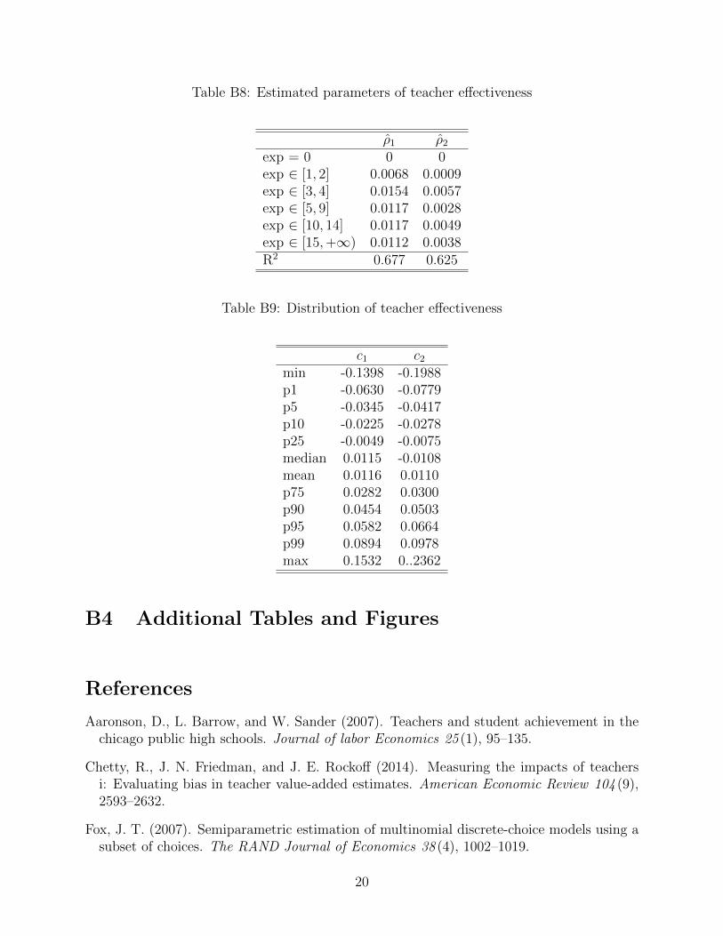
identification. The distribution of effectiveness measures estimated with this achievement
model is summarized in Table B9 and Figure B2. Next, we describe the alternative model,
and its estimation and identification. Finally, we show that the effectiveness measures we
obtain from both models are strongly correlated and that our auxiliary models used in our
structural estimation are robust to the choice of effectiveness measures.
5
B2.3.1 Achievement Model 1 (Main)
The effectiveness measures used in our empirical analysis are estimated using the following
achievement model:
Akt = γZskt +
∑i:SGkt=SG
Tit
2∑n=1
I (τk = n) (ρnxit + vin) + εkt (8)
= γZskt +
∑i:SGkt=SG
Tit
2∑n=1
I (τk = n) ρnxit + ϕkt (9)
where Akt is achievement (measured as the standardized Math test score) of student k in
year t. The vector Zskt contains the following: a cubic polynomial of previous year’s test
scores, interacted with grade fixed effects; a cubic polynomial of previous year’s average test
scores for k’s cohort in the school, interacted with grade fixed effects; a set of student charac-
teristics, including gender, race and ethnicity, disability status, English-language status, and
socioeconomic status; the same average characteristics for student k’s cohort; cohort size;
grade-by-school fixed effects; and year fixed effects. The variable εkt is an i.i.d. unobservable
component of achievement, idiosyncratic to each student and year. SGkt (SGTit) denotes the
school-grade of student k (teacher i) in year t. The variable τk equals 1 for low-achieving
students and 2 for high-achieving ones; we consider a student to be low-achieving if their test
score in the previous year is below the grade-specific median in the state, and high-achieving
otherwise. The contribution of teacher i to the achievement of a student of type n ∈ 1, 2is ρnxit + vin, where xit denotes i’s education and experience in year t and vin is the part
unexplained by xit.
The achievement model in (8) assumes that all teachers in a given school-grade contribute
to the achievement of all students in the same school-grade. We make this choice to be able
to allow xit to directly enter teacher effectiveness (since experience has been shown to affect
teacher effectiveness (Wiswall 2013), especially in the first years of a teacher’s career (Rockoff
2004)), even if we do not observe all the teacher-student classroom links in the data. Model
(8) allows us to identify the component of teacher effectiveness that depends on a teacher’s
experience and education.
Constructing our measures of effectiveness (ci1, ci2) requires estimating vin and ρn for
n ∈ 1, 2. We make the following two assumptions:
A1. εkt is i.i.d. with mean 0 and variance σ2ε .
A2. Cov(εkt, vin) = 0 ∀k, i, t, n : SGTit = SGkt. This implies that there is no sorting on
unobservables of teachers across school-grades within a district. Although there is no direct
6
test of this assumption, in Section B3.3, we combine the approaches of Chetty et al. (2014)
and Rothstein (2010) and we do not find evidence of non-random sorting.
Estimation Procedure: Model 1
1. Given A1 and A2, we estimate γ and ρn via OLS on equation (8), to obtain γ and ρn.
2. With the estimated γ and ρn, we can then estimate vin using an empirical Bayes
estimator similar to the one of Kane and Staiger (2008) which we adapt to take into
account the structure of our data.
(a) Let
ϕkt = Akt − γZskt −
∑i:SGkt=SG
Tit
2∑n=1
ρnxitI(τk = n). (10)
The quantity ϕkt is an estimate for ϕkt, i.e.,
ϕkt ≡∑
i′:SGkt=SGTi′t
2∑n=1
vi′nI(τk = n) + εkt.
Let KSGTitnbe the number of achievement type-n students in the school-grade that
i belongs to. For each teacher i we define, for n ∈ 1, 2
vint =1
KSGTitn
∑k:SGkt=SG
Tit
ϕktI (τk = n) (11)
which is an estimate of ∑i′:SGT
i′t=SGTit
vi′n +1
KSGTitn
∑k:SGkt=SG
Tit
εkt.
This quantity corresponds to the average test score residuals of type-n students
in teacher i’s school-grade in year t, conditional on observables Zskt and the char-
acteristics x of all teachers in the same school-grade in t.
(b) We form a weighted average of the residuals vintt by weighting each vint by
$int =KSGT
itn∑
tKSGTitn
, so that residuals corresponding to more observations receive
more weight:
vin =∑t
$intvint (12)
7
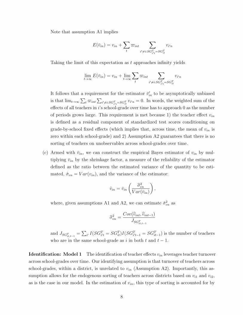
Note that assumption A1 implies
E(vin) = vin +∑t
$int
∑i′ 6=i:SGT
i′t=SGTit
vi′n
Taking the limit of this expectation as t approaches infinity yields
limt→∞
E(vin) = vin + limt→∞
∑t
$int
∑i′ 6=i:SGT
i′t=SGTit
vi′n
It follows that a requirement for the estimator v′in to be asymptotically unbiased
is that limt→∞∑
t$int
∑i′ 6=i:SGT
i′t=SGTitvi′n = 0. In words, the weighted sum of the
effects of all teachers in i’s school-grade over time has to approach 0 as the number
of periods grows large. This requirement is met because 1) the teacher effect vin
is defined as a residual component of standardized test scores conditioning on
grade-by-school fixed effects (which implies that, across time, the mean of vin is
zero within each school-grade) and 2) Assumption A2 guarantees that there is no
sorting of teachers on unobservables across school-grades over time.
(c) Armed with vin, we can construct the empirical Bayes estimator of vin by mul-
tiplying vin by the shrinkage factor, a measure of the reliability of the estimator
defined as the ratio between the estimated variance of the quantity to be esti-
mated, σvn = V ar(vin), and the variance of the estimator:
vin = vin
(σ2vn
V ar(vin)
),
where, given assumptions A1 and A2, we can estimate σ2vn as
σ2vn =
Cov(vint, vint−1)
JSGTit,t−1
and JSGTit,t−1=∑
i′ I(SGTi′t = SGT
it)I(SGTi′t−1 = SGT
it−1) is the number of teachers
who are in the same school-grade as i in both t and t− 1.
Identification: Model 1 The identification of teacher effects vin leverages teacher turnover
across school-grades over time. Our identifying assumption is that turnover of teachers across
school-grades, within a district, is unrelated to vin (Assumption A2). Importantly, this as-
sumption allows for the endogenous sorting of teachers across districts based on vi1 and vi2,
as is the case in our model. In the estimation of vin, this type of sorting is accounted for by
8
the school-grade fixed effects included in Zskt.
Teacher turnover across school-grades allows us to identify vin from vin for all i and n. In
particular, we can stack all the equations (12) for all I teachers and n = 1, 2, forming a system
of 2I equations (where I is the total number of teachers) in 2I unknowns (vini,n∈1,2).Identification is achieved if the rank condition of the system is satisfied, i.e., if the coefficient
matrix of the system is full-rank.
In practice, this requires that the set i′ : SGTi′t = SGT
it∀t is empty for all i, which
means that there are no two teachers who teach the same school-grade in all t. When this
is the case, the system (and the vin for all i and n) is perfectly identified. In our data,
i′ : SGTi′t = SGT
it∀t is empty for 75% of teachers, for whom we can precisely estimate
(vi1, vi2) . For the remaining 25% of teachers, i′ := SGTi′t = SGT
it∀t is non-empty, and our
estimated vin is the average of vi′n for i′ : SGTi′t = SGT
it∀t.
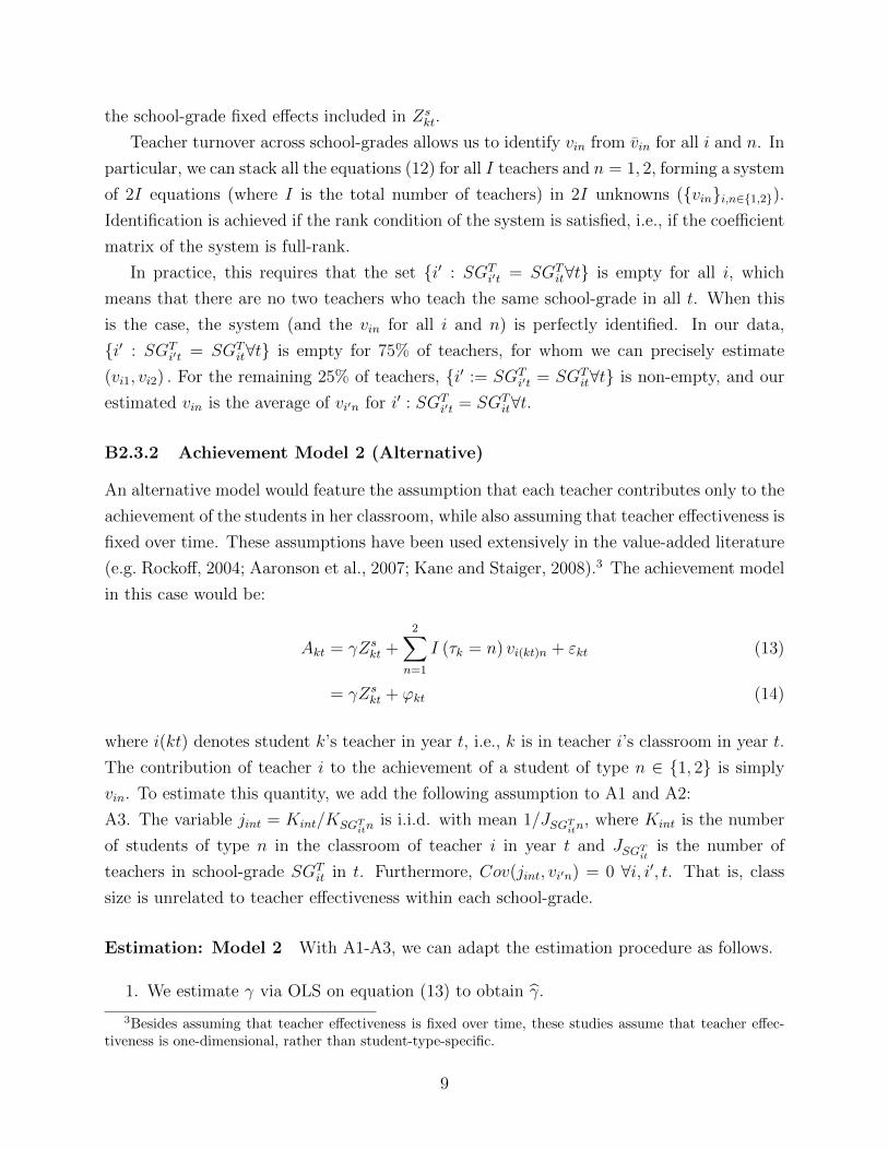
B2.3.2 Achievement Model 2 (Alternative)
An alternative model would feature the assumption that each teacher contributes only to the
achievement of the students in her classroom, while also assuming that teacher effectiveness is
fixed over time. These assumptions have been used extensively in the value-added literature
(e.g. Rockoff, 2004; Aaronson et al., 2007; Kane and Staiger, 2008).3 The achievement model
in this case would be:
Akt = γZskt +
2∑n=1
I (τk = n) vi(kt)n + εkt (13)
= γZskt + ϕkt (14)
where i(kt) denotes student k’s teacher in year t, i.e., k is in teacher i’s classroom in year t.
The contribution of teacher i to the achievement of a student of type n ∈ 1, 2 is simply
vin. To estimate this quantity, we add the following assumption to A1 and A2:
A3. The variable jint = Kint/KSGTitnis i.i.d. with mean 1/JSGTitn, where Kint is the number
of students of type n in the classroom of teacher i in year t and JSGTit is the number of
teachers in school-grade SGTit in t. Furthermore, Cov(jint, vi′n) = 0 ∀i, i′, t. That is, class
size is unrelated to teacher effectiveness within each school-grade.
Estimation: Model 2 With A1-A3, we can adapt the estimation procedure as follows.
1. We estimate γ via OLS on equation (13) to obtain γ.
3Besides assuming that teacher effectiveness is fixed over time, these studies assume that teacher effec-tiveness is one-dimensional, rather than student-type-specific.
9
2. We construct
ϕ′kt = Akt − γZskt (15)
which is an estimate for∑2
n=1 vi(kt)nI(τk = n) + εkt. For each teacher i, we define, for
n ∈ 1, 2
v′int=1
KSGTitn
∑k:SGkt=SG
Tit
ϕ′ktI (τk = n) (16)
which is an estimate of∑
i′:SGTit=SGTi′t
ji′ntvi′n +1
KSGTitn
∑k:SGkt=SG
Tit
εkt (17)
3. We form a weighted average of v′intt, with the same weights $int as before:
v′in =∑t
$intv′int
Assumption A1. implies
E(v′in) = vin∑t
$int
JSGTit+∑t
$int
JSGTit
∑i′:SGTit=SG
Ti′t
vi′n
Taking the limit of this expectation as t approaches infinity implies
limt→∞
E(v′in) = vin∑t
$int
JSGTit+ lim
t→∞
∑t
$int
JSGTit
∑i′:SGTit=SG
Ti′t
vi′n
It follows that the estimator
¯v′in =1∑
t$intJSGT
it
v′in (18)
is asymptotically unbiased if limt→∞∑
t$intJSGT
it
∑i′:SGTit=SG
Ti′tvi′n = 0. As before, this
requirement implies that the weighted average of the effects of all teachers in i’s school-
grade over time has to approach 0 as the number of periods grows large. Assumption
A2 and the fact that we are conditioning on school-grade fixed effects guarantees that
this is the case asymptotically.
4. Finally, we construct the empirical Bayes estimator for vin as
v′in = ¯v′in
(σ2′vn
V ar(¯v′in)
)
10
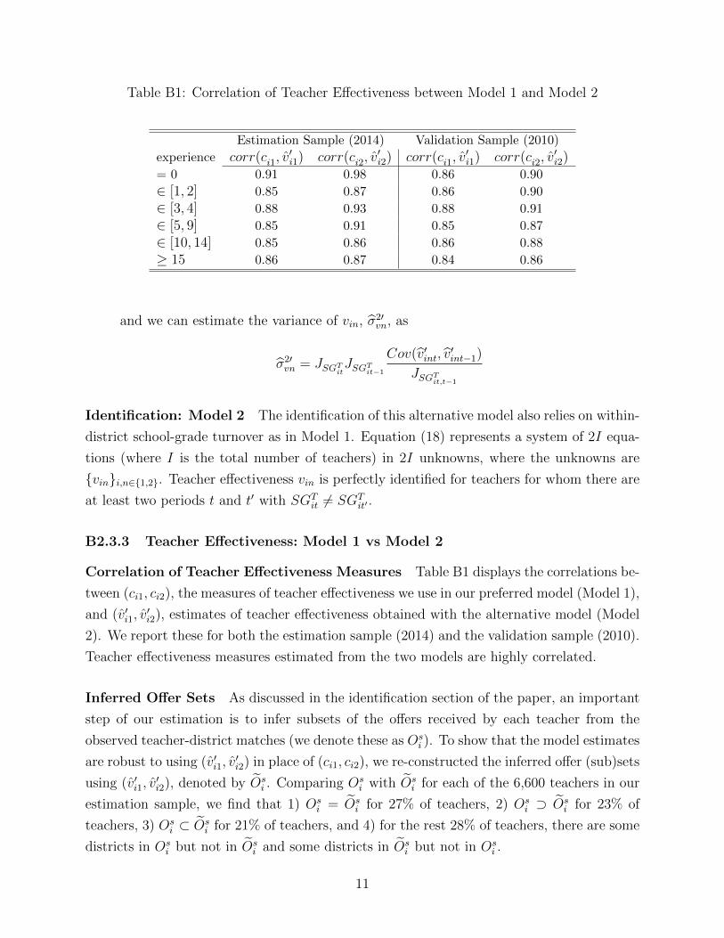
Table B1: Correlation of Teacher Effectiveness between Model 1 and Model 2
Estimation Sample (2014) Validation Sample (2010)
experience corr(ci1, v′i1) corr(ci2, v
′i2) corr(ci1, v
′i1) corr(ci2, v
′i2)
= 0 0.91 0.98 0.86 0.90
∈ [1, 2] 0.85 0.87 0.86 0.90
∈ [3, 4] 0.88 0.93 0.88 0.91
∈ [5, 9] 0.85 0.91 0.85 0.87
∈ [10, 14] 0.85 0.86 0.86 0.88
≥ 15 0.86 0.87 0.84 0.86
and we can estimate the variance of vin, σ2′vn, as
σ2′vn = JSGTitJSGTit−1
Cov(v′int, v′int−1)
JSGTit,t−1
Identification: Model 2 The identification of this alternative model also relies on within-
district school-grade turnover as in Model 1. Equation (18) represents a system of 2I equa-
tions (where I is the total number of teachers) in 2I unknowns, where the unknowns are
vini,n∈1,2. Teacher effectiveness vin is perfectly identified for teachers for whom there are
at least two periods t and t′ with SGTit 6= SGT
it′ .
B2.3.3 Teacher Effectiveness: Model 1 vs Model 2
Correlation of Teacher Effectiveness Measures Table B1 displays the correlations be-
tween (ci1, ci2), the measures of teacher effectiveness we use in our preferred model (Model 1),
and (v′i1, v′i2), estimates of teacher effectiveness obtained with the alternative model (Model
2). We report these for both the estimation sample (2014) and the validation sample (2010).
Teacher effectiveness measures estimated from the two models are highly correlated.
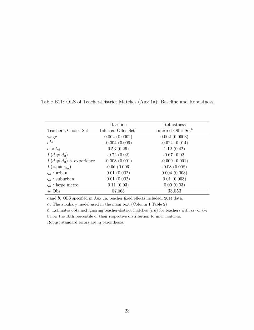
Inferred Offer Sets As discussed in the identification section of the paper, an important
step of our estimation is to infer subsets of the offers received by each teacher from the
observed teacher-district matches (we denote these as Osi ). To show that the model estimates
are robust to using (v′i1, v′i2) in place of (ci1, ci2), we re-constructed the inferred offer (sub)sets
using (v′i1, v′i2), denoted by Os
i . Comparing Osi with Os
i for each of the 6,600 teachers in our
estimation sample, we find that 1) Osi = Os
i for 27% of teachers, 2) Osi ⊃ Os
i for 23% of
teachers, 3) Osi ⊂ Os
i for 21% of teachers, and 4) for the rest 28% of teachers, there are some
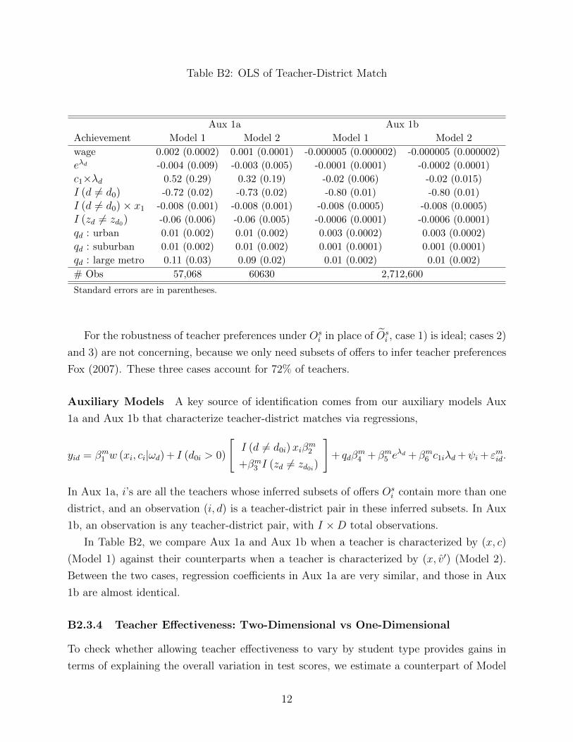
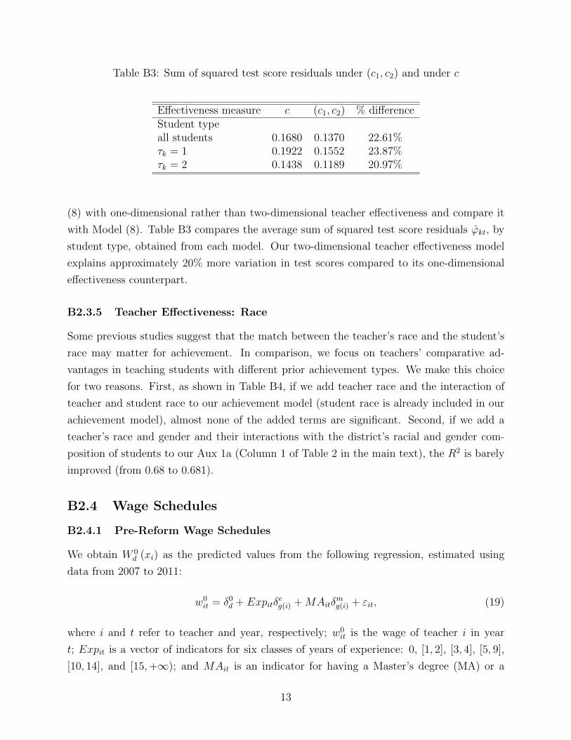
(8) with one-dimensional rather than two-dimensional teacher effectiveness and compare it
with Model (8). Table B3 compares the average sum of squared test score residuals ϕkt, by
student type, obtained from each model. Our two-dimensional teacher effectiveness model
explains approximately 20% more variation in test scores compared to its one-dimensional
effectiveness counterpart.
B2.3.5 Teacher Effectiveness: Race
Some previous studies suggest that the match between the teacher’s race and the student’s
race may matter for achievement. In comparison, we focus on teachers’ comparative ad-
vantages in teaching students with different prior achievement types. We make this choice
for two reasons. First, as shown in Table B4, if we add teacher race and the interaction of
teacher and student race to our achievement model (student race is already included in our
achievement model), almost none of the added terms are significant. Second, if we add a
teacher’s race and gender and their interactions with the district’s racial and gender com-
position of students to our Aux 1a (Column 1 of Table 2 in the main text), the R2 is barely
improved (from 0.68 to 0.681).
B2.4 Wage Schedules
B2.4.1 Pre-Reform Wage Schedules
We obtain W 0d (xi) as the predicted values from the following regression, estimated using
data from 2007 to 2011:
w0it = δ0
d + Expitδeg(i) +MAitδ
mg(i) + εit, (19)
where i and t refer to teacher and year, respectively; w0it is the wage of teacher i in year
t; Expit is a vector of indicators for six classes of years of experience: 0, [1, 2], [3, 4], [5, 9],
[10, 14], and [15,+∞); and MAit is an indicator for having a Master’s degree (MA) or a
13
Table B4: Estimates of achievement model in equation (13), obtained controlling for teachers’(T) and students’ (S) race/ethnicity indicators and their interactions
τ = 1 τ = 2(1) (2)
Black S -0.056∗∗∗ -0.067∗∗∗
(0.003) (0.003)
Hisp S -0.007∗∗ -0.022∗∗∗
(0.003) (0.003)
Asian S 0.053∗∗∗ 0.081∗∗∗
(0.004) (0.004)
Black T -0.001(0.005)
Black T * Black S -0.008 -0.019∗
(0.006) (0.010)
Hisp T -0.010∗ -0.006(0.005) (0.005)
Hisp T * Hisp S 0.007 0.008(0.007) (0.009)
Asian T 0.003 0.004(0.007) (0.008)
Asian T * Asian S 0.015 0.022(0.017) (0.016)
Observations 3360517 3635942
higher degree. The parameter δ0 can be interpreted as the average wages for teachers with
zero experience and without a MA; with δeg(i) normalized to 0 for those with zero experience,
δeg(i) is the average wage premium for teachers in each of the higher experience category,
relative to those with zero experience with the same education; and δm is the wage premium
for teachers who have a MA.
We estimate the intercept δ0d separately for each district. Trading off the accuracy of our
wage schedules with power, we estimate the coefficients δe and δm by groups of districts,
defined as follows:
1. For the 35 large districts (i.e., those with at least 10 teachers in each experience and
education category), each group corresponds to a district.
14
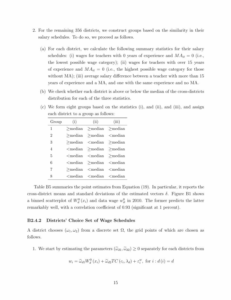
2. For the remaining 356 districts, we construct groups based on the similarity in their
salary schedules. To do so, we proceed as follows.
(a) For each district, we calculate the following summary statistics for their salary
schedules: (i) wages for teachers with 0 years of experience and MAit = 0 (i.e.,
the lowest possible wage category); (ii) wages for teachers with over 15 years
of experience and MAit = 0 (i.e., the highest possible wage category for those
without MA); (iii) average salary difference between a teacher with more than 15
years of experience and a MA, and one with the same experience and no MA.
(b) We check whether each district is above or below the median of the cross-districts
distribution for each of the three statistics.
(c) We form eight groups based on the statistics (i), and (ii), and (iii), and assign
each district to a group as follows:
Group (i) (ii) (iii)
1 ≥median ≥median ≥median
2 ≥median ≥median <median
3 ≥median <median ≥median
4 <median ≥median ≥median
5 <median <median ≥median
6 <median ≥median <median
7 ≥median <median <median
8 <median <median <median
Table B5 summaries the point estimates from Equation (19). In particular, it reports the
cross-district means and standard deviations of the estimated vectors δ. Figure B1 shows
a binned scatterplot of W 0d (xi) and data wage w0
it in 2010. The former predicts the latter
remarkably well, with a correlation coefficient of 0.93 (significant at 1 percent).
B2.4.2 Districts’ Choice Set of Wage Schedules
A district chooses (ω1, ω2) from a discrete set Ω, the grid points of which are chosen as
follows.
1. We start by estimating the parameters (ωd1, ωd2) ≥ 0 separately for each districts from
wi = ωd1W0d (xi) + ωd2TC (ci, λd) + εwi , for i : d (i) = d
15
Table B5: Cross-district Summary of Pre-Reform Wage Schedules
Cross-district Mean Cross-district Std Dev.
δ0 34,686.8 3,286.1
δe: [1, 2] 1,719.2 598.3
[3, 4] 3,939.1 1,103.3
[5, 9] 8,227.8 1,536.6
[10, 14] 14,644.0 2,348.5
≥15 21,235.4 3,063.4
δm(MA) 7,008.5 2,456.6
Figure B1: Relationship between W 0d (xi) and w0
it
correlation = .93
40
50
60
70
80
Wid0
40 50 60 70 80wit
0
Note: Binned scatterplot of W 0d (xi) and w0
it using wage data from 2010.
16
where wi is the observed 2014 wage for teacher i working in district d (i : d (i) = d),
W 0d (xi) is defined as in Section B2.4.1, and teacher contribution TC (ci, λd) is given by
TC (ci, λd) = λdci1 + (1− λd) ci2.
2. Based on the estimated (ωd1, ωd2)d , we choose a set of equally spaced grid points
that provides a good coverage of the empirical distribution in the data:
Aaronson, D., L. Barrow, and W. Sander (2007). Teachers and student achievement in thechicago public high schools. Journal of labor Economics 25 (1), 95–135.
Chetty, R., J. N. Friedman, and J. E. Rockoff (2014). Measuring the impacts of teachersi: Evaluating bias in teacher value-added estimates. American Economic Review 104 (9),2593–2632.
Fox, J. T. (2007). Semiparametric estimation of multinomial discrete-choice models using asubset of choices. The RAND Journal of Economics 38 (4), 1002–1019.
20
Figure B2: Distribution of teacher effectiveness
0
5
10
15
20
Den
sity
-.2 -.1 0 .1 .2
c1 c2
Kane, T. J. and D. O. Staiger (2008). Estimating teacher impacts on student achievement:An experimental evaluation. NBER Working Paper .
Rockoff, J. E. (2004). The impact of individual teachers on student achievement: Evidencefrom panel data. American Economic Review 94 (2), 247–252.
Rothstein, J. (2010). Teacher quality in educational production: Tracking, decay, and studentachievement. The Quarterly Journal of Economics 125 (1), 175–214.
21
Table B10: Teacher and District Characteristics (2010)
A. Teacher Characteristics All x1< 3 x1≥ 10x1: Experience 15.6 (9.6) 1.6 (0.5) 20.2 (7.7)
x2: MA or above 0.55 (0.50) 0.05 (0.22) 0.66 (0.48)
10c1 0.11 (0.25) 0.07 (0.27) 0.11 (0.25)
10c2 0.12 (0.30) 0.06 (0.32) 0.12 (0.29)
Corr (c1, c2) 0.65 - -
# Teachers 6,741 391 4,675
B. District Characteristics All λd 1st Quartile λd 4th Quartile