Page 1
1
Equilibrium Modeling of Combined Heat and Power Deployment
Anand Govindarajana, Seth Blumsack
a*
a Leone Family Department of Energy and Mineral Engineering, Pennsylvania State University
University Park, PA 16802
*Corresponding author. Tel: +1 (814) 863-7597, Fax: +1 (814) 865-3248
E-mail address: [email protected]
Abstract
Combined heat and power (CHP) generates electricity and heat from the same fuel source and
can provide these services at higher equivalent conversion efficiency relative to grid-purchased
electricity and stand-alone steam production. Previous work has focused on the economic factors
and optimal operation strategy that influence the decision to install a single CHP unit. Our
approach is to assess the economic potential for CHP in electricity-market equilibrium
framework, accounting for the impact that CHP adoption will have on energy prices. We utilize a
statistical model of electricity supply and pricing to estimate zonal supply curves for
transmission constrained electricity markets. We couple the above model of electricity prices
with simulated usage of CHP in different types of buildings, using the Philadelphia area as a case
study. Incremental installations of CHP reduce the electricity demand from the grid, thus
reducing wholesale electricity prices. The net present value from CHP is modeled as a function
of wholesale electricity prices, and thus decreases with each additional unit of CHP installed.
Under a range of operational assumptions and fuel prices, substantial CHP deployment could be
achieved without reducing returns to the point where incremental CHP installations would
become uneconomic.
Keywords: Combined Heat and Power, Energy Efficiency, Electricity market modeling
1. Introduction
About two-thirds of the fuel used for electricity generation is wasted as heat; this is in
addition to the transmission and distribution losses (U.S. Environmental Protection Agency
2008a). Electricity generation is the single largest contributor of greenhouse gas emissions in the
U.S (U.S Environmental Protection Agency 2010), so the inefficiency of central-station power
generation is a contributing factor to emissions. Combined heat and power captures and reuses
the waste heat and provides a viable alternative to centralized electricity generation for
qualifying applications (Siler-Evans et al 2012; Strachan and Farrell 2006; Strachan and Farrell
2006).
Combined heat and power (CHP) also known as cogeneration, is the onsite production of
electricity where the co-produced heat is captured and utilized for space heating, cooling, and
Page 2
2
other site specific applications. The most important characteristic of CHP is the on-site
generation of electricity and heat from the same fuel source. Commonly, this fuel is natural gas
but other fuels such as biomass have potential for utilization in CHP systems as well. Compared
to the conventional method of providing electricity through the power grid and producing onsite
heat using a gas fired boiler system, CHP can yield substantial equivalent efficiency gains.
A shortcoming with deploying CHP in commercial buildings is the utilization of the
rejected heat during summer. However, the heat from CHP is used to run an absorptive chiller to
provide air conditioning. This is called tri-generation or combined cooling, heat and power
(CCHP). In a case study of small-scale CHP in a hospital, the absorptive chillers were cost-
effective addition to the CHP system (Siler-Evans et al 2012). This provides the flexibility of
using the heat for space heating in the winter and cooling in the summer. Distributed generation,
including CHP, decreases the dependence on power grid and provides reliable power supply
along with cost savings and emissions reduction benefits (Zerriffi et al 2007). CHP can act as a
backup source of power during power outages caused by natural disasters or breakdowns in the
electricity grid. CHP can be linked with district heating schemes in municipalities or university
campuses and this practice is proven practical in countries like Denmark and Finland (Kelly and
Pollitt 2010; Unterwurzacher 1992).
Despite the potential benefits, CHP’s share of electricity generation in U.S is less than 10
per cent. In comparison, CHP’s share of total electricity production in countries like Finland and
Denmark is about 38 percent and 52 percent respectively(International Energy Agency 2008).
Some of the hurdles for CHP adoption in the U.S. include electricity rate structures,
interconnection issues with the grid, tax treatment and technical barriers related to the flexibility
of CHP systems (Oak Ridge National Lab 2008). From an investor’s perspective, adopting CHP
is a business decision and economic viability is a crucial factor.
Several studies use net present value and payback period as a measure of feasibility in
evaluating the application of CHP to different types of commercial buildings. A general finding
is that the combination of low fuel prices and high electricity prices is generally advantageous
for distributed generation, including CHP (King and Morgan, 2007). In a study comparing the
use of CHP and CCHP units to a supermarket, the CCHP system had better primary energy
saving potential but had a higher payback period (Maidment et al 2001). The higher payback
period was attributed to the capital costs associated with the absorptive chiller but better payback
period is achieved as the size of the chiller unit increased and as the demand for the chiller unit
increases. An economic feasibility study of applying CCHP systems to a hospital show that the
project and low payback period and high net present value (Ziher and Poredos 2006). A study
conducted to study the emission reduction potential of CHP systems in seven types of
commercial buildings showed that hospitals had the highest reduction of CO2, NOx, and CH4
emissions (Pedro J. Mago and Smith 2012). In addition, schools and small offices showed an
increase in primary energy consumption.
Page 3
3
The application of CHP systems to various commercial buildings requires understanding
of the difference in energy consumption patterns and thermal and electric ratios. In a report
assessing the market potential for cogeneration, commercial buildings types were ranked based
on the size, hours of operation, system configuration and concurrence in thermal and electric
loads (Lawrence Berkeley National Lab 1991). The report suggests that CHP does not offer
similar benefits to all types of buildings. Hospitals are the best candidates among commercial
buildings for deploying CHP because of the large size, continuous operation throughout the year
and high electricity and heating demand.
Previous work has focused on the economic factors and optimal operation strategy that
influence the decision to install a single CHP unit or assess the technical potential of CHP. Our
approach is to assess the economic potential for CHP in electricity-market equilibrium
framework, accounting for the impact that CHP adoption will have on energy prices. We couple
an econometric model of electricity prices with simulated usage of CHP in different types of
buildings, using the Philadelphia area, which falls under the PECO zone of PJM electricity
market, as a case study. We find that under certain operational and fuel-price scenarios, the
equilibrium level of economical CHP deployment is substantially lower than the technical
potential. Incremental installations of CHP reduce the demand for electricity provided by the
grid, thus reducing wholesale electricity prices. The net present value from CHP (i.e., the
discounted value of the energy cost savings) is modeled as a function of wholesale electricity
prices, and thus decreases with each additional unit of CHP installed.
The remainder of this paper is organized as follows - Section 2 introduces some
background work on supply curve modeling and developing a working model of electricity
prices and fuels utilization in the PECO zone, which will reflect changes in electricity prices with
various levels of CHP deployment. Section 3 describes the equilibrium modeling of CHP
deployment. Section 4 gives a brief description of the case study along with the relevant data and
methodology. Section 5 discusses the results of the case study and section 6 provides
conclusions.
2. Background on supply curve modeling
In modern restructured electricity markets, such as the PJM market in the United States,
market prices change frequently and are influenced primarily by the level of electricity demand.
Prices are set by the supply offer of the generating unit that clears the market – i.e., the last unit
dispatched to equate total system supply and demand. Shifts in demand will affect the set of
generating units dispatched and thus the clearing price in the electricity market. Our approach
models the impact of CHP adoption on electricity demand in Greater Philadelphia, and thus the
wholesale price of electricity along with the utilization of different fuels to serve aggregate
demand for grid-provided power in Greater Philadelphia. We do not consider impacts on prices
for capacity or ancillary services in this paper, but the costs of these services would be expected
to rise and fall along with actual or projected electricity demand.
Page 4
4
Modeling electricity prices and fuels utilization in a transmission-constrained electricity
markets is complex. Actual supply curves based on cost data from the generation owners or
transmission system operators are not public information. Much of the existing literature
estimates short run supply curves using data from the Emissions and Generation Resource
Integrated Database (eGRID 2007) published by the U.S. Environmental Protection Agency
(Newcomer and Apt 2009; Newcomer et al. 2008). Figure 1 is the estimated short run supply
curve for PJM electricity market using the above methodology.
Figure 1 - Short run supply curve for PJM electricity market. Each marker represents a generator.
These supply curves built in previous work typically model coal generators as being
dispatched before natural gas generators in PJM electricity market. This scenario, however, is
changing as the recent discovery of Marcellus shale gas reserves has led to a decrease in gas
prices in the Mid-Atlantic region. The share of natural gas for power generation has been
growing and the share of coal has been declining. Also, coal fired power plants are increasingly
facing regulatory hurdles and increased costs related to air emissions of various pollutants
(Newcomer and Apt 2009).
A second drawback with this approach is that it ignores transmission constraints on the
electricity network. Transmission constraints can induce a different marginal fuel and prices at
two different locations within in the same interconnected power system (Sahraei-Ardakani et al
2012). For example, in a location with high demand, oil will be the marginal fuel and therefore
higher electricity prices as compared to a location with relatively lower demand where coal or
gas will be on the margin and lower electricity prices.
0
50
100
150
200
250
300
350
400
450
0 50 100 150 200
Short
run M
argin
al c
ost
($/M
Wh)
PJM Demand (GW)
Oi
Gas Coal
Baseload Shoulder Peak
Page 5
5
To address this issue, we draw on recent work (Sahraei-Ardakani et al 2012) that
estimates statistical models of electricity supply and pricing in transmission constrained
electricity markets. These estimated supply curves incorporate the transmission constraints in an
electricity network unlike the short run marginal cost curves (like the one shown in Figure 1) that
are estimated using individual plant level data. The approach taken by Sahraei-Ardakani, et al., is
to construct an econometric model that estimates prices on a sub-system or “zonal” basis, using
publicly-available data on fuel prices and electricity loads. The fuel on the margin in a zone (i.e.,
the fuel whose price best explains variations in electricity price over a relevant range of
demands) is a function of the zonal demand, total system demand and the relative fuel prices.
Supply curves for each type of fuel (coal, gas and oil) are determined and each segment
represents the influence of the fuel on the electricity price.
Figure 2 - Supply curve with transmission constraints for PECO zone estimated by Sahraei-
Ardakani et al (2012)
The estimated supply curve is piecewise linear with three segments associated with the
three different fuels (coal, gas and oil; other fuels are generally price-setters in the PJM system).
Thresholds based on demand levels where the marginal input fuel switches differentiate the three
segments. The threshold value when the marginal fuel switches from coal to gas is ‘3846 MW’
and ‘8140 MW’ for gas to oil. There is a small discontinuity when the fuel at the margin changes
3 4 5 6 7 80
50
100
150
200
Load in PECO (GW)
Pri
ce i
n P
EC
O (
$/M
Wh
)
Page 6
6
from coal to gas indicating that marginal cost of producing electricity from gas is comparable to
coal plants. This transition point is modeled using a fuzzy logic type of approach (Sahraei-
Ardakani et al 2012) where the marginal fuel is actually a mixture of two different fuels, such as
coal and gas. Saharei-Ardakani, et al (2012) also suggest that the gap could be widened with
changes in relative fuel prices i.e. decline in natural gas prices or increase in coal prices.
3. Model description
A large-scale deployment of CHP will decrease the demand for grid-provided electricity
and thus will decrease location-based prices in wholesale electricity markets. Unlike previous
work examining investment incentives for a single CHP unit, or estimating technical potential for
CHP deployment, our goal is to estimate an equilibrium model of CHP deployment, using the
Philadelphia zone within the PJM electricity market as a case study. Our approach represents an
equilibrium model in that it incorporates feedbacks in electricity prices on the net present value
of additional CHP installations. In other words, we estimate the level of CHP deployment such
that additional investments in CHP in that region will not be beneficial or a marginal CHP
investment will have a negative net present value.
The zonal electricity price is a function of the zonal demand in the grid and a decrease in
demand will decrease the electricity prices. The savings from CHP is a function of the real-time
electricity prices, so a decrease in the demand will tend to lower savings, holding the natural gas
price constant. The demand reduction depends on the number of CHP units installed. Figure 3
explains the model of equilibrium CHP market deployment.
Page 7
7
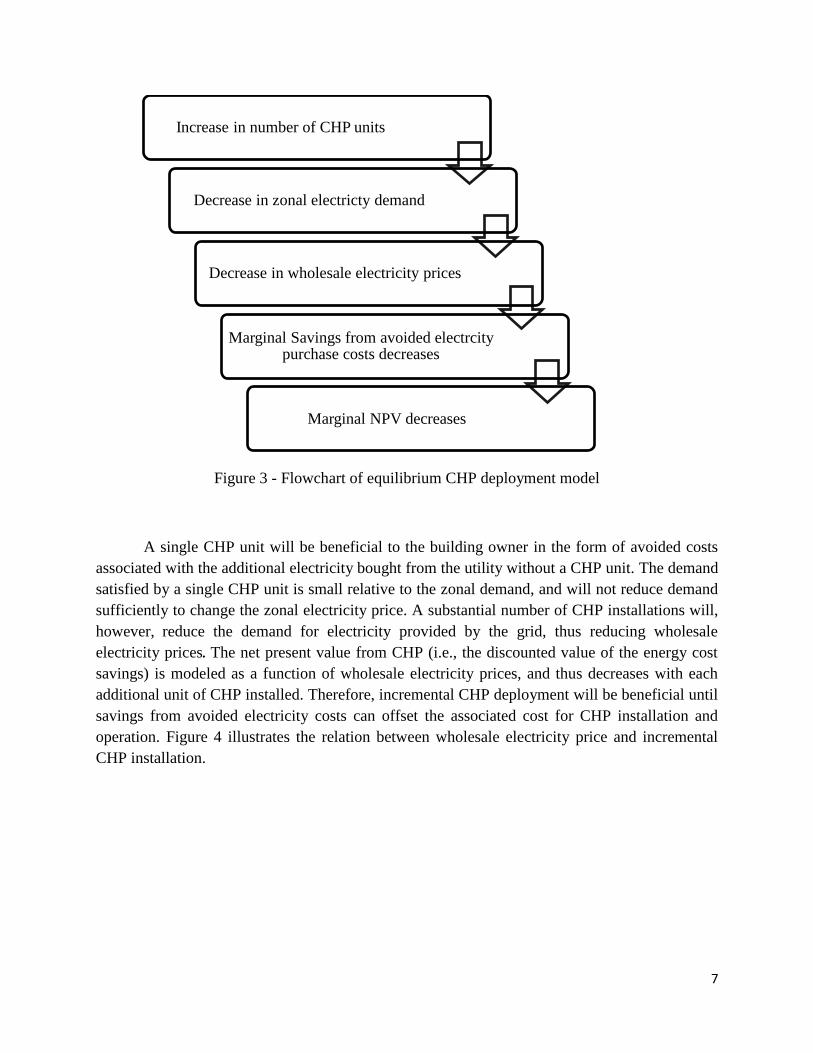
Figure 3 - Flowchart of equilibrium CHP deployment model
A single CHP unit will be beneficial to the building owner in the form of avoided costs
associated with the additional electricity bought from the utility without a CHP unit. The demand
satisfied by a single CHP unit is small relative to the zonal demand, and will not reduce demand
sufficiently to change the zonal electricity price. A substantial number of CHP installations will,
however, reduce the demand for electricity provided by the grid, thus reducing wholesale
electricity prices. The net present value from CHP (i.e., the discounted value of the energy cost
savings) is modeled as a function of wholesale electricity prices, and thus decreases with each
additional unit of CHP installed. Therefore, incremental CHP deployment will be beneficial until
savings from avoided electricity costs can offset the associated cost for CHP installation and
operation. Figure 4 illustrates the relation between wholesale electricity price and incremental
CHP installation.
Increase in number of CHP units
Decrease in zonal electricty demand
Decrease in wholesale electricity prices
Marginal Savings from avoided electrcity purchase costs decreases
Marginal NPV decreases
Page 8
8
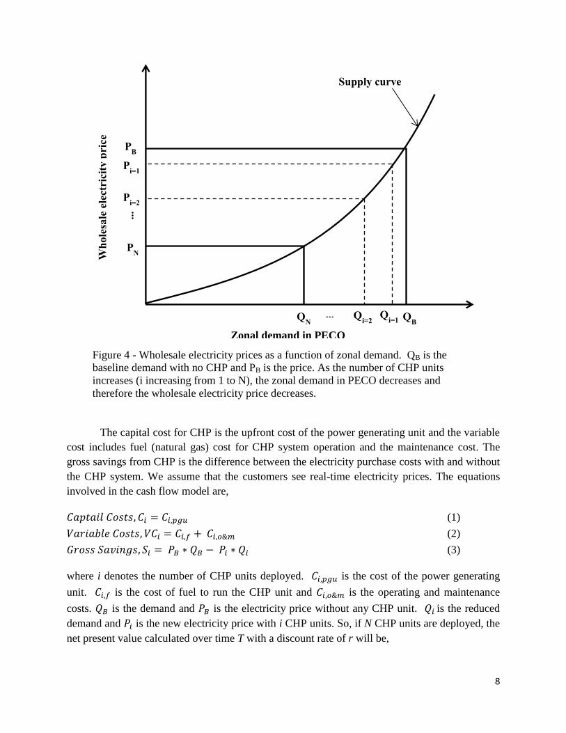
The capital cost for CHP is the upfront cost of the power generating unit and the variable
cost includes fuel (natural gas) cost for CHP system operation and the maintenance cost. The
gross savings from CHP is the difference between the electricity purchase costs with and without
the CHP system. We assume that the customers see real-time electricity prices. The equations
involved in the cash flow model are,
(1)
(2)
(3)
where i denotes the number of CHP units deployed. is the cost of the power generating
unit. is the cost of fuel to run the CHP unit and is the operating and maintenance
costs. is the demand and is the electricity price without any CHP unit. is the reduced
demand and is the new electricity price with i CHP units. So, if N CHP units are deployed, the
net present value calculated over time T with a discount rate of r will be,
Figure 4 - Wholesale electricity prices as a function of zonal demand. QB is the
baseline demand with no CHP and PB is the price. As the number of CHP units
increases (i increasing from 1 to N), the zonal demand in PECO decreases and
therefore the wholesale electricity price decreases.
PN
...
Qi=2
Zonal demand in PECO
Wh
ole
sale
ele
ctri
city
pric
e
Supply curve
PB
Pi=2
Pi=1
QB Q
N Q
i=1 ...
Page 9
9
∑ {∑ (
)
} (4)
The savings potential of CHP depends on the zonal electricity price and operation
strategy of the CHP unit. At some level of CHP deployment, the savings will be equal to the
costs (discounted). At this equilibrium point, a marginal CHP investment will not be beneficial
and will have a net present value of zero.
4. Description of the case study
This study focuses on the deployment of single-user CHP among various types of
commercial buildings in Philadelphia, in Southeastern Pennsylvania. A typical single-user
building CHP installation would represent a few megawatts or less of power generation capacity.
Larger installations (tens of megawatts), as would be typical of industrial applications, are not
considered in our analysis. Philadelphia falls in the PECO zone of the PJM electricity market.
Primarily due to transmission constraints, prices in the PECO zone have historically been higher
than average for the PJM market as a whole.
Data on Philadelphia’s commercial building stock was obtained from the CoStar database
(Econsult Corporation 2011). While the database does not capture the universe of commercial
buildings in Philadelphia, it does provide the best available representation of the region’s
commercial building stock and the distribution of building stock among different building types.
Table 1 shows the number of buildings in eight types of commercial buildings in Philadelphia.
Table 1 - Commercial buildings stock in Philadelphia
Rank1
Building Type Number of buildings
1 Hospital 50
2 Large Hotel 74
3 Restaurant 29
4 Large Office 284
5 Supermarket 51
6 School2 63
7 Motel 22
8 Warehouse 439
1 Priority rankings for CHP deployment in different types of commercial buildings developed by
Lawrence Berkley National Laboratory(Lawrence Berkeley National Lab 1991)
Page 10
10
2 The Costar database did not include information on the school buildings in the region and this
number was obtained from National Center for Education Statistics. Online at
<http://nces.ed.gov/datatools/>.
4.1 Building Hourly loads
Comprehensive energy demand profiles of buildings are not commonly recorded. The
Building - CHP Screening tool (BCHP), developed by Oak Ridge National Lab, was used to
develop hourly electricity, heating and cooling demand profiles for the eight types of buildings
under study (Oak Ridge National Lab 2005). The BCHP tool estimates energy demand profiles
for various types of commercial buildings based on user-defined parameters such as building
dimensions, location and occupancy schedules. Input parameters for the eight types of
commercial building were obtained from by U.S Department of Energy Commercial Reference
Building Models of the National Building Stock (National Renewable Energy Lab 2011). For
each type of building, three scenarios were developed – Baseline without CHP, CHP system
following thermal loads (CHP-FTL) and CHP system following electrical load (CHP-FEL) (P. J.
Mago, Fumo, and Chamra 2009).
The baseline scenario is a reference case without any CHP units installed. For CHP
following thermal load, the system is operated to maximize the delivery of thermal load required
at the site for various processes such as space heating, space cooling, dehumidification and other
site related applications. In the process of operating the CHP unit to meet thermal demands,
some amount of electricity is generated. The recovered heat from the CHP system will displace
much, if not all, of the fossil fuel required that would have been required in a conventional boiler
for the site and the electricity produced meets some of the demand. For CHP following electric
load, the CHP system operates to meet the site’s electricity demand. In general, this is not
economical because onsite generation of electricity from CHP cannot compete with central
station generation of electricity on a cost per kWh basis. In addition, the recovered heat does not
match with the thermal demand; hence a complete advantage of the fuel savings is not realized.
Table 2 provides the area, building occupancy schedule and hours of generator operation
used in the BCPH tool for each type of building. We assumed the generators operated when the
electricity demand was high. The periods of high demand for each type of building was
estimated based on the baseline case simulation results.
Page 11
11
Table 2 - Buildings occupancy schedule and peak-electricity demand periods
Table 3 compares the energy intensities from the BCHP tool and the energy intensities
for buildings in Mid-Atlantic region obtained from the Commercial Building Energy
Consumption Survey (Energy Information Administration 2006). The CBECS is a nation-wide
survey of energy consumption of commercial buildings in the U.S. Energy intensities for certain
building types were missing under the Mid-Atlantic census division. The missing values were
obtained from Buildings Energy Data Book (US Department of Energy 2011). There are some
substantial differences between the energy intensities from CBECS and from BCHP. In
particular, BCHP’s estimates of energy intensity for supermarkets and warehouses are more than
20% higher than estimates from CBECS.
Building type Area
(m2)
Hours of generator
operation Building occupancy schedule
Hospital 22422 8 am to 6 pm weekdays - 24 hours
weekends - 24 hours
Large Office 46320 9 am to 3 pm weekdays - 7 am to 8 pm
weekends - closed
Large Hotel 11345 7 am to 2pm,
6 pm to 9 pm
weekdays - 24 hours
weekends - 24 hours
Motel 4014 7 am to 11 am,
7 pm to 9 pm
weekdays - 24 hours
weekends - 24 hours
Supermarket 4181 8 am to 5 pm weekdays - 8 am to 8 pm
weekends - 8 am to 8 pm
Restaurant 511 10 am to 7 pm weekdays - 9 am to midnight
weekends - 9 am to midnight
School 19572 10 am to 2 pm weekdays - 8 am to 10 pm
weekends - closed
Warehouse 4835 9 am to 4 pm weekdays – 8 am to 6 pm
weekends - closed
Page 12
12
Table 3 - Energy Intensity Validation
Building Type
Energy Intensity
from CBECS
(1000 Btu/SF)
Energy
Intensity from
BCHP (1000
Btu/SF)
Hospital 214 201
Large Office 81 64
Large Hotel 110 113
Small Hotel/Motel 75 102
Supermarket 74 89
Restaurant 198 172
Secondary School 80 69
Warehouse 49 72
The BCHP tool calculates the generator sizing using the DOE-2 sizing run. The sizing
depends on the maximum load for each building type since we model the generator to operate
during periods of high demand. Table 4 gives the generator sizing for each building type.
Table 4 - Generator sizing for each type of building
Building Type Generator Size(kW)
Hospital 1500
Large Hotel 420
Restaurant 30
Large Office 1820
Supermarket 200
School 550
Small Hotel/Motel 125
Warehouse/Flex- industrial 100
Page 13
13
3.2 Average Costs estimates for a CHP system
The costs associated with a CHP system include capital costs, and operating costs such as
fuel and maintenance. It is assumed that all the CHP units run on natural gas. Average cost
estimates for a typical CHP unit were obtained from the U.S. Environmental Protection Agency
(Environmental Protection Agency 2008b). Table 5 gives an average capital and operation and
maintenance cost for a typical CHP system. The natural gas consumption under each operational
strategy is obtained from BCHP tool to estimate the fuel cost.
Table 5 - Average cost estimates for a typical CHP system
Capital Cost ($/kW)
1200
Incremental O&M cost ($/kWh) 0.01
3.3 Methodology
We model CHP deployment according to the priority rankings developed by the
Lawrence Berkley National Laboratory (Lawrence Berkeley National Lab 1991). Our analysis
assumes that CHP units will be installed at the most advantageous sites first (according to the
LBNL rankings) followed by deployment at progressively less advantageous sites. We thus
assume that CHP units will be installed first in all the hospitals (which are ranked the most
advantageous single-use cases for CHP) followed by large hotels and so on, as shown in Table 1.
Reflecting a limitation in the CoStar data, we assume that building types have homogeneous
thermal and electric load profiles within type and those demand profiles are well-represented by
the BCHP tool. The BCHP tool is utilized to generate hourly CHP usage profiles for each
building type. For each deployment scenario, hourly CHP usage is aggregated across all
simulated CHP installations; this represents the electricity demand taken off the PJM electric
grid in each hour. We thus reduce hourly demand in the PECO zone of the PJM electricity
markets (using demand in 2010 as the baseline) with every CHP unit deployed and estimate the
zonal price change with incremental CHP units deployed. Figure 5 shows the load duration
curves for the baseline case and the reduced demand with CHP units following thermal load
(FTL) and electric load (FEL) for all 1,012 CHP units corresponding to the commercial building
stock represented in the CoStar database. CHP-FEL has more on-site generation compared to
CHP-FTL and hence higher displacement of grid-provided electricity.
Page 14
14
Figure 5 - Load duration curves for a) Baseline demand, b) CHP-FTL, c) CHP- FEL
Reductions in grid-provided electricity, however, are reasonably modest in magnitude no
matter what operational strategy is modeled (FEL or FTL). The average demand for electricity
from the grid reduces from 4879 MW (baseline) to 4820 MW in case of CHP-FTL and 4720
MW in case of CHP-FEL. The standard deviation for base line, CHP-FTL and CHP-FEL are
1011, 1009 and 1025 MW respectively.
Large-scale CHP deployment might affect both natural gas and electricity prices, in
opposite directions (since CHP would increase demand for natural gas while decreasing demand
for grid-provided electricity). Natural gas prices affect the operating costs of CHP and also the
zonal electricity prices (hence savings). We capture uncertainty in the price of natural gas using
three gas price scenarios ($2/mm Btu, $4/ mm Btu and $8/ mm Btu). Prices for coal and oil
(other fuels utilized in the Philadelphia region) are assumed to remain constant (coal - $2 / mm
Btu, oil – $10.667/ mm Btu). The net present value on a CHP investment is calculated for three
natural gas price scenarios for a 10-year period with a discount rate 10%. The return on
investment is calculated assuming first year (2010) savings are achieved every year.
1000 2000 3000 4000 5000 6000 7000 80002000
3000
4000
5000
6000
7000
8000
9000
FTL
Baseline
FEL
Load
(M
Wh
)
Hours
Page 15
15
5. Results
The technical potential for CHP in Philadelphia is substantial. Incremental installations of
CHP, however, reduce the demand for electricity provided by the grid, thus reducing wholesale
electricity prices. The return on incremental investment is a function of the electricity prices,
decreases as the number of CHP units installed increases. Figure 6 shows the price duration
curves corresponding to the load duration curves in figure 5.
Figure 6 - Price duration curves for a) Baseline demand, b) CHP-FEL, c) CHP- FTL.
Fuel prices are assumed to be, coal - $2 / mm Btu, gas - $8/mm Btu, oil – $10/ mm Btu.
With natural gas prices of $2/mm Btu and $4/mm Btu (and $2/mm Btu coal price) we do
not observe substantial differences in the effects on the price duration curve arising from 1,012
CHP installations operated according to FEL and FTL. The results suggest that price reduction
(and savings) is sensitive to natural gas prices and the operational strategy of CHP. In particular,
we find that the impacts of CHP adoption will have larger impacts on the electricity price
duration curve under high gas-price scenarios. This is due primarily to the reductions in peak-
time electricity demand. We also find that operating CHP units in FEL mode has a larger impact
400 1000 2000 3000 4000 5000 6000 7000 8000
20
30
40
50
60
70
80
90
100
110
Hours
Pri
ce (
$/M
Wh
)
Baseline
FEL
FTL
100 200 300 400100
150
200
Page 16
16
on the electricity price duration curve (through larger reductions in demand for grid-provided
electricity) than does operating CHP units in FTL mode.
The gross savings from a CHP unit are the avoided costs from purchasing additional
electricity bought from the utility without a CHP unit (net savings would incorporate the cost of
natural gas to fuel the CHP unit, plus other operational or maintenance costs). As shown in figure
5 and 6, there will be decrease in demand and price every hour in a year. We estimate the hourly
savings using equation (3) and aggregate it to get yearly savings from avoided electricity costs.
Figures 7, 8 and 9 show gross electricity cost savings as a function of the number of CHP units
deployed and the operational strategy (FEL or FTL). The figures calculate gross electricity cost
savings over a 10-year period under three gas-price scenarios ($2/mm Btu, $4/ mm Btu and $8/
mm Btu). Higher savings were achieved with higher $8/mm Btu natural gas price as there will be
more savings from avoided electricity costs as compared to a $2/mm Btu natural gas price. The
savings from CHP-FEL is higher since there will be more onsite electricity generation, hence
higher avoided electricity costs as compared to CHP-FTL. The total savings curve tends to
flatten as number of CHP unit deployed increases indicating that the incremental savings from
CHP decreases.
Figure 7 - Total Savings with a $2/mm Btu natural gas price
100 200 300 400 500 600 700 800 900 10000
0.5
1
1.5
2
2.5
3x 10
7
# CHP units
Tot
al S
avin
gs (
$)
FTL
FEL
Number of CHP units
Gro
ss S
avin
gs
($)
Page 17
17
Figure 8 - Total Savings with a $4/mm Btu natural gas price
100 200 300 400 500 600 700 800 900 10000
1
2
3
4
5
6
7x 10
7
# CHP units
Tot
al S
avin
gs ($
)
FTL
FEL
100 200 300 400 500 600 700 800 900 10000
2
4
6
8
10
12
14
16
18x 10
7
# CHP units
To
tal
Sa
vin
gs
($)
FTL
FEL
Number of CHP units
Number of CHP units
Gro
ss S
av
ing
s ($
) G
ross
Savin
gs
($)
Page 18
18
Figure 9 - Total Savings with a $8/mm Btu natural gas price
After about 300 CHP installations, the savings from CHP-FEL decreases for a $2/mm
Btu natural gas price (figure 7). This happens because of low zonal electricity prices resulting
because of substantial demand taken off the grid coupled with lower natural gas price. At this
point, the price of electricity from the utility is cheaper than generating on-site electricity from
CHP. This means that any further deployment of CHP-FEL will not be beneficial to the building
owner.
Figures 10, 11 and 12 show the incremental energy cost savings (which we term
“marginal savings” for CHP installations, for the three natural gas price scenarios and the two
CHP operation strategies. The marginal savings from CHP-FTL decreases with increase in the
number of CHP units for all three price scenarios. Marginal savings from CHP-FEL actually
increase for deployment in hospitals (the first 50 CHP units), since the savings in grid-purchased
electricity is large compared to the impact on LMPs in the PECO zone. As less advantageous
CHP units are deployed, the marginal savings begins to decrease more rapidly.. Marginal savings
flattens out once roughly 100 to 300 CHP units are deployed, reflecting a combination of lower
reductions in the demand for grid-provided electricity and a shift inwards of electricity demand
towards the less-elastic portion of the PECO supply curve.
100 200 300 400 500 600 700 800 900 10000
1
2
3
4
5
6x 10
5
# CHP units
Mar
gin
al S
avin
gs (
$)
FTL
FEL
Number of CHP units
Marg
inal
Savin
gs
($)
Page 19
19
Figure 10 - Marginal savings with a $2/mm Btu natural gas price
Figure 11 - Marginal savings with a $4/mm Btu natural gas price
100 200 300 400 500 600 700 800 900 10000
1
2
3
4
5
6x 10
5
# CHP units
Mar
gina
l Sav
ings
($)
FTL
FEL
100 200 300 400 500 600 700 800 900 10000
1
2
3
4
5
6
7
8
9x 10
5
# CHP units
Mar
gina
l Sav
ings
($)
FTL
FEL
Number of CHP units
Number of CHP units
Marg
inal
Savin
gs
($)
Marg
inal
Savin
gs
($)
Page 20
20
Figure 12 - Marginal savings with a $8/mm Btu natural gas price
For all levels of the natural gas price, we observe fluctuations in the incremental savings
from aditional CHP installations. This effect appears most prominent under the FEL mode of
operation. The reason for this behavior is related to the mixture of coal and natural gas on the
margin in the PECO zone of PJM (which we referred to as the “fuzzy gap” in section 2),
especially in those scenarios with low gas prices. The supply curve model in section 2 was
estimated with a natural gas price of $8/mm Btu, a coal price of $2/mm Btu and an oil price of
$10.66/mm Btu. With these fuel prices, the partial supply curves associated with coal, gas, oil
and the threshold level is well-defined. With low natural gas prices, the cost of generating
electricty from gas is as cheap as generating electricty from coal with a low natural gas price (say
$2/mm Btu). The threshold between the coal portion of the supply curve and the natural-gas
portion of the supply curve becomes less well-defined. The fuel at the margin keeps switching
between coal and natural gas leading to fluctuations in electricty prices. The savings from CHP
is a function of the zonal elctricty price and hence there are fluctuations in incremental savings.
Also, the deviations are minimal when the natural gas price is $8/mm Btu which suggests that
the supply curve model works better for higher natural gas prices. The fluctuations are minimal
with CHP-FTL as compared to CHP-FEL because the demand reduction is not high enough to
create siginificant flucutuations in electricty prices.
The net present value modeled as a function of electricty prices is estimated using
equation (4), assuming a 10-year decision horizon and a 10% annual discount rate. Figures 13,
14 and 15 show how the marginal NPV for CHP installations changes with the three price
scenarios. While we observe some fluctuations in the NPV of an incremental CHP installation at
low levels of CHP utilization, we generally observe a decline in the NPV of the marginal CHP
unit, as anticipated. Not only does marginal NPV decreases with incremental CHP installations
and under certain operational and fuel-price scenarios, the equilibrium level of economical CHP
deployment is substantially lower than the technical potential. With a $2/mmBtu natural gas
price the operating costs of a CHP unit is less but at the same time the savings is also less
because of lower electricty costs. With a $8/mmBtu natural gas price, the high operating costs is
offset by the higher savings from avoided electricty prices.
Page 21
21
Figure 13 - Marginal NPV with a $2/mm Btu natural gas price
Figure 14 - Marginal NPV with a $4/mm Btu natural gas price
100 200 300 400 500 600 700 800 900 1000-0.5
0
0.5
1
1.5
2
2.5
3
3.5x 10
6
# CHP units
Mar
gina
l NP
V (
$))
FTL
FEL
Number of CHP units
Number of CHP units
Marg
inal
NP
V (
$)
Marg
inal
NP
V (
$)
Page 22
22
Figure 15 - Marginal NPV with a $8/mm Btu natural gas price
For the natural gas price scenarios of $2 and $4 /mm Btu the marginal NPV declines
quickly under the FTL operational strategy, approaching zero by the time 100 to 150 CHP units
are installed and operating. Thus, if all CHP units are operated according to FTL, then the
economic extent of the market in Philadelphia is around one-tenth of the technical potential for
these lower gas prices scenarios. In the case of CHP-FEL, for a gas price of $2/ mm Btu the
marginal NPV beomes zero after 282 units are installed; for a gas price of $4/ mm Btu the
marginal NPV becomes zero for after 424 CHP units are installed. These points suggests that any
further CHP deployment will not be benefiical. The marginal NPV doesn’t cross zero with a
$8/mm Btu for CHP-FEL and CHP-FTL. Thus, if all CHP units are operated according to FEL,
the economic potential is larger (around three to four times as large as under FTL operations) but
still substantially smaller than the technical potential in the lower gas price scenarios.
We draw three policy-relevant lessons from our analysis of CHP deployment in the
Philadelphia region. First, higher gas prices in and of themselves do not economically
disadvantage CHP – the spark spread (difference between gas and electricity prices) is the more
relevant variable, as also pointed out by King and Morgan (2005). Our model of electricity
pricing in Philadelphia and the operational costs of single-user CHP suggests that increases in
natural gas prices will disproportionally affect electricity prices relative to CHP operational
100 200 300 400 500 600 700 800 900 10000
2
4
6
8
10
12
14
16
18x 10
5
# CHP units
Mar
gina
l NP
V (
$))
FTL
FEL
Number of CHP units
Marg
inal
NP
V (
$)
Page 23
23
costs. Second, the operational strategy adopted for CHP matters just as much in determining
profitable deployment levels as does the fuel price. Perhaps driven by high peak-time prices for
electricity in Philadelphia, we find that an operational strategy of electric load following (FEL)
yields larger economic savings than thermal load following (FTL) when CHP has relatively low
levels of adoption. At higher levels of adoption, FTL may be a more economical operational
strategy when fuel prices are low (see Figures 7, 10 and 13). Third, ecxept in the highest fuel-
price scenarios, the economic potential for CHP in the Philadelphia region is substantially
smaller than the technical potential. This conclusion suggests that additional policy measures to
support CHP adoption (including the feed-in tariff policy option suggested by Siler-Evans et al,
2012) would need to be justified by further analysis of the social benefits of CHP in reducing
greenhouse-gas emissions; improving local air quality; or improving the resiliency of electrical
networks.
6. Conclusions
CHP represents a near-term solution to improve energy efficiency and reduce greenhouse
gas emissions but its adoption has been slow for various reasons. The Philadelphia region has
significant technical potential for CHP and with the recent development of Marcellus Shale, CHP
could represent a substantial consumer of regionally-produced natural gas. While previous
analyses have modeled the individual decision to adopt CHP based on electricity market prices
and other relevant variables, our analysis utilizes a statistical model of electricity supply and
pricing in the Philadelphia region is used to capture relevant feedbacks between adoption rates,
electricity pricing and the economic viability of incremental CHP adoption. Marginal savings
and marginal NPV curves were estimated for three gas price scenarios and two CHP operation
strategies (i.e., CHP-FTL and CHP-FEL). The marginal savings and marginal NPV decrease as
the number of CHP units increase for all three-gas price scenarios and two CHP operation
strategies. This study suggests that the priority rankings for CHP deployment are important
considering a large-scale adoption of CHP in a region. The results suggests that higher natural
gas prices and hence higher electricity prices, is favorable for CHP adoption. Under a range of
operational assumptions and fuel prices, substantial CHP deployment could be achieved without
reducing returns to the point where existing and incremental CHP installations would become
uneconomic. The results of this study leads to a number of policy related questions such as how
the natural gas demand created by a large-scale deployment of CHP might affect regional natural
gas prices, assessing the importance of CHP as a source of reliable power, the associated
environmental benefits, and factors affecting individual decisions to install CHP.
Bibliography
Cardona, E., and A. Piacentino, 2004. A Validation Methodology for a Combined Heating Cooling and Power
(CHCP) Pilot Plant. Journal of Energy Resources Technology 126 (4): 285. doi:10.1115/1.1803849.
Econsult Corporation, 2011. The Market for Commercial Property Energy Retrofits in the Philadelphia Region.
Online at < http://www.econsult.com/GPIC_report.pdf>
Page 24
24
Hendriks, Chris, and Kornelis Blok, 1996. Regulation for Combined Heat and Power in the European Union.
Proceedings of the International Energy Agency Greenhouse Gases: Mitigation Options Conference 37 (6–8) (June):
729–734. doi:10.1016/0196-8904(95)00247-2.
International Energy Agency, 2008. Combined Heat and power: Evaluating the Benefits of Greater Global
Investment. Online at < http://www.iea.org/media/files/chp/chp_report.pdf.>
Kelly, Scott, and Michael Pollitt, 2010. An Assessment of the Present and Future Opportunities for Combined Heat
and Power with District Heating (CHP-DH) in the United Kingdom. Energy Efficiency Policies and Strategies with
Regular Papers. 38 (11) (November): 6936–6945. doi:10.1016/j.enpol.2010.07.010.
King, Douglas E., and M. Granger Morgan, 2007. Customer-Focused Assessment of Electric Power Micro grids.
Journal of Energy Engineering 133 (3) (September): 150–164. doi:10.1061/(ASCE)0733-9402(2007)133:3(150).
Lawrence Berkeley National Lab, 1991. 481 Prototypical Commercial Buildings for 20 Urban Market Areas
(Technical Documentation of Building Loads Database Developed for the GRI Cogeneration Market Assessment
Project). Report No. LBL-29798. Online at <http://gundog.lbl.gov/dirpubs/29798.pdf.>
Lemar Jr., Paul L, 2001. The Potential Impact of Policies to Promote Combined Heat and Power in US Industry.
Energy Policy 29 (14) (November): 1243–1254. doi:10.1016/S0301-4215(01)00070-2.
Mago, P. J., N. Fumo, and L. M. Chamra, 2009. Performance Analysis of CCHP and CHP Systems Operating
Following the Thermal and Electric Load. International Journal of Energy Research 33 (9) (July): 852–864.
doi:10.1002/er.1526.
Mago, Pedro J., and Amanda D. Smith, 2012. Evaluation of the Potential Emissions Reductions from the Use of
CHP Systems in Different Commercial Buildings. Building and Environment 53 (July): 74–82.
doi:10.1016/j.buildenv.2012.01.006.
Maidment, G.G, X Zhao, and S.B Riffat, 2001. Combined Cooling and Heating Using a Gas Engine in a
Supermarket. Applied Energy 68 (4) (April): 321–335. doi:10.1016/S0306-2619(00)00052-0.
National Renewable Energy Laboratory, 2011. U.S. Department of Energy Commercial Reference Building Models
of the National Building Stock. Online at <http://www.nrel.gov/docs/fy11osti/46861.pdf >
National Center for Education Statistics (NCES). Online at <http://nces.ed.gov/datatools/>. Accessed April 5, 2012
Newcomer, Adam, and Jay Apt, 2009. Near-Term Implications of a Ban on New Coal-Fired Power Plants in the
United States. Environmental Science & Technology 43 (11) (June): 3995–4001. doi:10.1021/es801729r.
Newcomer, Adam, Seth A. Blumsack, Jay Apt, Lester B. Lave, and M. Granger Morgan, 2008. Short Run Effects of
a Price on Carbon Dioxide Emissions from U.S. Electric Generators. Environmental Science & Technology 42 (9)
(May): 3139–3144. doi:10.1021/es071749d.
Oak Ridge National Lab, 2008. Combined heat and power: Effective Energy Solutions for a Sustainable Future.
ORNL/TM-2008/224. Online at <
http://www1.eere.energy.gov/manufacturing/distributedenergy/pdfs/chp_report_12-08.pdf>
Oak Ridge National Lab,2005. BCHP Screening Tool, Version 2.0.1. Online at
<http://www.coolingheatingpower.org/about/bchp-screening-tool.php.> Accessed November 12, 2011
Page 25
25
PJM Interconnection, 2012. Historical metered load data. Online at < http://www.pjm.com/markets-and-
operations/ops-analysis/historical-load-data.aspx>. Accessed February 21, 2012.
Sahraei-Ardakani, Mostafa, Seth Blumsack, and Andrew Kleit, 2012. Distributional Impacts of State-level Energy
Efficiency Policies in Regional Electricity Markets. Energy Policy 49 (October): 365–372.
doi:10.1016/j.enpol.2012.06.034.
Siler-Evans, Kyle, M. Granger Morgan, and Inês Lima Azevedo, 2012. Distributed Cogeneration for Commercial
Buildings: Can We Make the Economics Work? Energy Policy 42 (March): 580–590.
doi:10.1016/j.enpol.2011.12.028.
Strachan, Neil, and Alexander Farrell, 2006. Emissions from Distributed Vs. Centralized Generation: The
Importance of System Performance. Energy Policy 34 (17) (November): 2677–2689.
doi:10.1016/j.enpol.2005.03.015.
US Department of Energy Mid-Atlantic Clean Energy Application Center, 2011. Pennsylvania Combined heat and
power baseline assessment. Online at < http://www.research.psu.edu/events/expired-
events/naturalgas/documents/dpg-white-paper.pdf>
US Department of Energy, Energy Information Administration (EIA), 2006. Commercial buildings energy
consumption survey (2003 data). Online at
<http://www.eia.doe.gov/emeu/cbecs/cbecs2003/detailed_tables_2003/detailed_tables_2003.html#enduse03>.
Accessed June 7, 2012.
US Department of Energy, 2011. Buildings Energy Data Book. Online at
<http://buildingsdatabook.eren.doe.gov/ChapterIntro3.aspx>. Accessed June 7, 2012
US Department of Energy, 2012. Combined Heat and Power: A Clean Energy Solution. Online at
<http://www1.eere.energy.gov/manufacturing/distributedenergy/pdfs/chp_clean_energy_solution.pdf>
US Environmental Protection Agency, 2010. Sources of greenhouse gas emissions. Online at <
http://www.epa.gov/climatechange/ghgemissions/sources.html> Accessed February 22, 2013.
US Environmental Protection Agency, 2007. Emissions & Generation Resource Integrated Database (eGRID)
Version 1.1 (2007 data). Online at < http://www.epa.gov/cleanenergy/energy-resources/egrid/>. Accessed July 10,
2011.
US Environmental Protection Agency, 2008a. Combined Heat and Power Partnership: Efficiency benefits. Online at
< http://www.epa.gov/chp/basic/efficiency.html>. Accessed April, 6 2012.
US Environmental Protection Agency, 2008b. Combined Heat and Power Partnership: Economic benefits. Online at
< http://www.epa.gov/chp/basic/efficiency.html>. Accessed April, 6 2012.
Unterwurzacher, Erich, 1992. CHP Development: Impacts of Energy Markets and Government Policies. Energy
Policy 20 (9) (September): 893–900. doi:10.1016/0301-4215(92)90124-K.
Zerriffi, Hisham, Hadi Dowlatabadi, and Alex Farrell, 2007. Incorporating Stress in Electric Power Systems
Reliability Models. Energy Policy 35 (1) (January): 61–75. doi:10.1016/j.enpol.2005.10.007.
Ziher, D., and A. Poredos, 2006. Economics of a Trigeneration System in a Hospital. Applied Thermal Engineering
26 (7) (May): 680–687. doi:10.1016/j.applthermaleng.2005.09.007.