2354 IEEE TRANSACTIONS ON POWER SYSTEMS, VOL. 34, NO. 3, MAY 2019
Equivalent Circuit Formulation for Solving ACOptimal Power Flow
Marko Jereminov , Member, IEEE, Amritanshu Pandey , Graduate Student Member, IEEE,and Larry Pileggi, Fellow, IEEE
Abstract—In this paper, we formulate and solve the ac optimalpower flow (AC-OPF) as an equivalent circuit problem in termsof current, voltage, and admittance state variables. The generatormodels are represented using conductance and susceptance statevariables, and the operational and network constraints are trans-lated to corresponding current/voltage constraints without loss ofaccuracy or generality. To understand the physics behind the op-timality conditions of the optimization problem, we extend thelinear adjoint circuit theory to translate them to equivalent circuitdomain. It is shown that the operating point that defines the equiv-alent circuit solution precisely represents an AC-OPF solution. Wethen further exploit the equivalent circuit representation to usepower flow simulation techniques to robustly solve the optimiza-tion problem. The efficiency of our approach is demonstrated forseveral AC-OPF benchmark test cases (up to 70 k buses) undernominal and congested operating conditions, and the runtime andscalability properties are presented.
Index Terms—AC optimal power flow, equivalent circuit,circuit formulation, circuit formalism, nonlinear optimization.
I. INTRODUCTION
THE AC Power Flow analysis, based on iteratively solvingthe nonlinear power mismatch equations, was first con-
ceived five decades ago [1], and still remains the standard anal-ysis for operation and planning of the transmission-level powergrids. Not long after the first power flow formulation was postu-lated, the Alternating Current Optimal Power Flow (AC-OPF)was introduced by Carpentier [2] and Dommel and Tinney in[3]. The motivation behind the first AC-OPF problem was tofind a steady-state operating point of a power system that min-imizes the cost of generated real power while satisfying theoperating, network and stability constraints. Most notably, thefinancial market is defined by nonlinear pricing, while the highlynonlinear ‘PQV’ based power mismatch equations characterizethe network constraints that model the electrical power sys-tem [4]. When both are combined with operating and stability
Manuscript received July 1, 2018; revised September 20, 2018 and November12, 2018; accepted December 15, 2018. Date of publication December 20, 2018;date of current version April 17, 2019. This work was supported in part by theDefense Advanced Research Projects Agency under Award FA8750-17-1-0059for the RADICS program and in part by the National Science Foundation un-der Contract ECCS-1800812. Paper no. TPWRS-01004-2018. (Correspondingauthor: Marko Jereminov.)
Color versions of one or more of the figures in this paper are available onlineat http://ieeexplore.ieee.org.
Digital Object Identifier 10.1109/TPWRS.2018.2888907
constraints, they create a daunting optimization problem withmany possible local optimal solutions [5]. For this reason, theclassical OPF is recognized as a NP hard problem to solve, and arobust technique that can solve for an optimal solution in a rea-sonable amount of time still does not exist [4]. FERC (FederalEnergy Regulatory Commission) has reported [4] that today’s“approximate-solution techniques may unnecessarily cost tensof billions of dollars per year” and “result in environmental harmfrom unnecessary emissions.”
Developing the robust and efficient methodology that cansolve for an optimal solution of the AC-OPF problem has beena prominent research challenge and was until recently basedon improving the local optimization algorithms [6]. The recentbreakthrough has been made by introduction of relaxation algo-rithms that claim to find the global optimal solution of AC-OPFin [7]–[11]. The most promising advancement is presented in[8], [9], where the authors use the Semi-Definite (SDP) andSecond-Order Cone (SOCP) Programing relaxation to handlethe non-convexities of the AC-OPF problem. The proposed re-laxation algorithms are demonstrated to be exact and yield thezero-duality gap for the initially examined test cases [8]. Unfor-tunately, this is not the case in general [5], [12], and as discussedin [5], the proposed SDP/SOCP relaxations succeed in solvingradial network configuration test cases but are exact for meshednetwork test cases when there is only one feasible solution [5],[12]. The other major drawbacks that further affect the recov-ery of the global optimum from the relaxed problems, such asthe inability to handle negative Lagrange multipliers caused bybounding line constraints, are discussed in [12].
Understanding and exploiting the physics of a power sys-tem is the key factor to robust simulation and relaxation al-gorithms [10]. Importantly, the inherent nonlinearity of thetraditionally used ‘PQV’ formulation due to the power mismatchequations represent the biggest impediment to the formulationand efficient solution [4]. Therefore, different formulations thathave been proposed since the introduction of AC-OPF problemmostly differ in the approaches used to characterize the net-work constraints [4]. Notably, it has been suggested [4] that thecurrent-voltage based (I-V) formulations with linear networkconstraints and local nonlinearities isolated at each bus, seem-ingly represents the most promising formulation for modelingof network constraints. However, efficient handling of genera-tor models that has previously shown to be challenging for I-Vformulations of transmission level powerflow simulations [13],[14] worsened in the optimization problem, causing numerical
JEREMINOV et al.: EQUIVALENT CIRCUIT FORMULATION FOR SOLVING AC OPTIMAL POWER FLOW 2355
instability to occur [14]. To address this, the authors in [14]have proposed the hybrid method, where the generator busesare modeled using power mismatch equations while the rest ofthe network is handled using current mismatch equations. Im-portantly, this and all of the proposed formulations are basedon the models that introduce other non-convexities in both theequality and inequality constraints. This keeps the OPF prob-lem highly nonlinear, as well as prevents the robust large-scaleoptimization of power systems due to the inability to efficientlyhandle the nonlinear constraints [4]. Therefore, the challengeremains to find a robust algorithm that is capable of solving thegeneralized AC-OPF problem with all the emerging and existinggrid technologies.
Recent advances in power system simulations have includedthe use of complex current and voltage state variables withinthe equivalent split-circuit framework for solving the powerflow[15]–[17]. This formulation has demonstrated that the equivalentcircuit formalism provides new insight into robustly analyzingthe complete powerflow simulation problem [16]. More impor-tantly, decades of research toward advancing circuit simulationmethods that are now capable of robustly simulating nonlinearcircuits with billions of nodes can be adapted and directly ap-plied to the analysis of power systems [18]. Thus, it is shownthat the generator model problems introduced by application ofthe I-V formulation can be successfully overcome, thereby al-lowing the robust scaling to massive-size transmission problems[17].
In this paper we propose a novel framework for solving theAC Optimal Power Flow problem in terms of equivalent split-circuit state variables as an extension of the recent advancementsin power flow analysis. The key contribution of the paper is therepresentation of the AC-OPF problem in terms of a nonlinearequivalent circuit problem. Importantly, the generator model isredefined (Section III) in terms of conductance and susceptancestate variables, where the negative conductance supplies thereal power to the circuit, while the susceptance represents aninductor or capacitor that supplies or absorbs the reactive powerrespectively. The objective of real power cost minimization isnow related to the network constraints through the generator ad-mittance state variables. This formulation does not encounter theconvergence problems as reported for existing I-V formulations[14].
As part of this formulation, a significant contribution is at-tributed to extending the theory for linear adjoint (dual) circuitsto modeling the steady-state nonlinearities at fixed frequencyintroduced by constant power models. We derive the adjointcircuits for constant power models in Section IV, and furthershow that coupled simulation of power flow and its adjoint cir-cuit with addition of other control circuits exactly maps thenecessary optimality conditions of the optimization problem.Therefore, if sufficient conditions are met, the circuit solutionexactly represents an optimal power flow solution.
Lastly, a supporting contribution is the development of cir-cuit simulation techniques to ensure the robust large-scale con-vergence of proposed circuit formulation. The overall resultis our algorithm, ESCAPE (Enhanced Simulation of Circuit-based AC-OPF Problem Equivalent), that is an extension of our
recently introduced powerflow circuit simulation methods [16],[17], with inclusion of diode limiting heuristics [20], [21] to pre-serve the robust and efficient convergence properties, scalableto any-size power grids.
The proposed framework is applied to solve the AC-OPF cir-cuit for congested and nominal (without congestion constraints)operating conditions of various available test cases (up to 70 kbuses), and the results are compared with traditional AC-OPFand SDP relaxed AC-OPF results in Section VI.
II. TRADITIONAL AC-OPF FORMULATIONS
Consider a power system given by the set of busesN , whereasset of generators G and load demands D are subsets of N ,that are further connected by a set of network elements, TX .The objective of traditional AC-OPF is to find a steady-statesolution of a power system that minimizes the cost function ofreal power generation, Fc(P G), defined throughout the paperas a quadratic function given by a set of coefficients {a, b, c}:
minP G
Fc (P G) =|G|∑
g=1
[ag + bgPG,g + cgP2G,g ] (1)
while satisfying the power balance equations (2), (3) and addi-tional operational constraints (4)–(7).
PG,(g∈G(i)) − PD,i = |Vi ||N |∑k=1
|Vk |(GY
ik cos θik + BYik sin θik
)(2)
QG,(g∈G(i)) − QD,i = |Vi ||N |∑k=1
|Vk |(GY
ik sin θik − BYik cos θik
)(3)
Pmin,g ≤ PG,g ≤ Pmax,g ∀g ∈ G (4)
Qmin,g ≤ QG,g ≤ Qmax,g ∀g ∈ G (5)
Vmin,i ≤ |Vi | ≤ Vmax,i ∀i ∈ N (6)
P 2e + Q2
e ≤ S2max,e ∀e ∈ TX (7)
where |Vi | and θi represent voltage magnitude and angle statevariables, whereas PG,(g∈G(i)) , PD,i , QG,(g∈G(i)) and QD,i aregenerated and demanded real and reactive powers at the ith busrespectively. Variable θik defines the voltage angle differencebetween buses i and k, while GY
ik and BYik represent the real and
imaginary parts of the bus admittance matrix. Each generatorin the set G is further defined by the operating bounds on realand reactive powers (Pmin, g , Pmax, g , Qmin, g and Qmax, g )given in (4) and (5), while the voltage magnitude of each busis bounded by the operating limits given in (6). Lastly, (7) rep-resents the thermal limits of a eth network branch, given formaximum apparent power flow bounds (Smax,e), where realand reactive power flows can be written as functions of ithand kth bus voltage magnitudes and angles connected by the
2356 IEEE TRANSACTIONS ON POWER SYSTEMS, VOL. 34, NO. 3, MAY 2019
branch e as:
Pe = |Vi |2GYik − |Vi | |Vk |
(GY
ik cos θik + BYik sin θik
)(8)
Qe = −|Vi |2BYik − |Vi | |Vk |
(BY
ik cos θik − GYik sin θik
)(9)
It is important to note that the AC-OPF problem formulatedusing the power mismatch equations in rectangular coordinatesseems to provide a less nonlinear (quadratic nonlinearities) for-mulation, and as such, is used for the relaxation approaches thatare proposed in [7]–[11]. It does, however, preserve the localoptimal solutions [5] and remains nonlinear and non-convexboth locally and within the network configuration that has a lin-ear nature in terms of current and voltage state variables (linearRLC network) [4].
III. DEFINING NETWORK AND OPERATIONAL CONSTRAINTS
USING EQUIVALENT CIRCUIT STATE VARIABLES
The equivalent circuit approach to generalized modeling ofpower flow was recently introduced in [15]–[17]. It was shownthat each of the power system components can be translated to anequivalent circuit model based on underlying relations betweencurrent and voltage state variables without loss of generality. Tofurther ensure the analyticity of nonlinear complex governingcircuit equations for solution via Newton Raphson, the equationsare split into real and imaginary parts and represented by twoequivalent sub-circuits, real and imaginary, that are coupled bycontrolled sources. The equivalent split-circuit representationof the most prominent powerflow models are described in [15],[16].
In this section we rederive the circuit model of a gener-ator based on the relationship between current, voltage andimpedance, as well as introduce the transmission line congestionconstraint based on maximum current limit. The two new mod-els incorporated within the powerflow split-circuit formulationdefine the network constraints of the circuit theoretic AC-OPFproblem.
A. Generator GB Macro-Model
Considering the VΓ and IG,g as the output complex voltageand complex current of the gth generator from the set G, oper-ating at a fundamental frequency, where the subscript index Γrepresents the corresponding bus index of the gth generator.
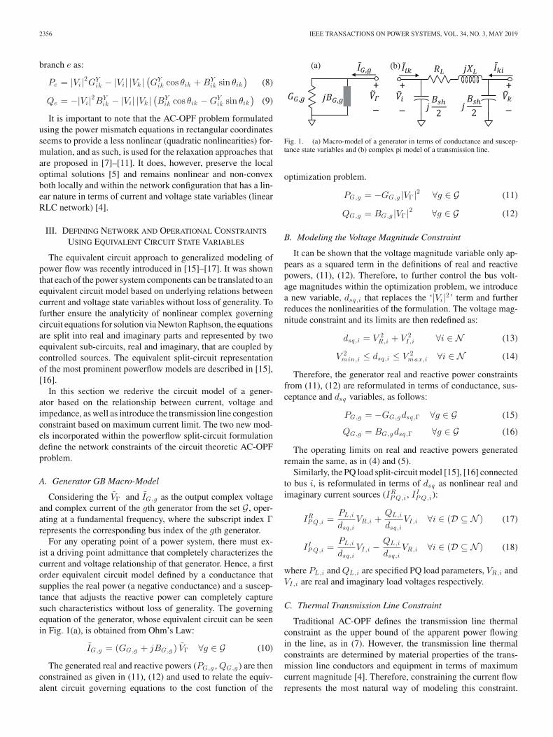
For any operating point of a power system, there must ex-ist a driving point admittance that completely characterizes thecurrent and voltage relationship of that generator. Hence, a firstorder equivalent circuit model defined by a conductance thatsupplies the real power (a negative conductance) and a suscep-tance that adjusts the reactive power can completely capturesuch characteristics without loss of generality. The governingequation of the generator, whose equivalent circuit can be seenin Fig. 1(a), is obtained from Ohm’s Law:
IG,g = (GG,g + jBG,g ) VΓ ∀g ∈ G (10)
The generated real and reactive powers (PG,g , QG,g ) are thenconstrained as given in (11), (12) and used to relate the equiv-alent circuit governing equations to the cost function of the
Fig. 1. (a) Macro-model of a generator in terms of conductance and suscep-tance state variables and (b) complex pi model of a transmission line.
optimization problem.
PG,g = −GG,g |VΓ |2 ∀g ∈ G (11)
QG,g = BG,g |VΓ |2 ∀g ∈ G (12)
B. Modeling the Voltage Magnitude Constraint
It can be shown that the voltage magnitude variable only ap-pears as a squared term in the definitions of real and reactivepowers, (11), (12). Therefore, to further control the bus volt-age magnitudes within the optimization problem, we introducea new variable, dsq,i that replaces the ‘|Vi |2’ term and furtherreduces the nonlinearities of the formulation. The voltage mag-nitude constraint and its limits are then redefined as:
dsq,i = V 2R,i + V 2
I ,i ∀i ∈ N (13)
V 2min,i ≤ dsq,i ≤ V 2
max,i ∀i ∈ N (14)
Therefore, the generator real and reactive power constraintsfrom (11), (12) are reformulated in terms of conductance, sus-ceptance and dsq variables, as follows:
PG,g = −GG,gdsq,Γ ∀g ∈ G (15)
QG,g = BG,gdsq,Γ ∀g ∈ G (16)
The operating limits on real and reactive powers generatedremain the same, as in (4) and (5).
Similarly, the PQ load split-circuit model [15], [16] connectedto bus i, is reformulated in terms of dsq as nonlinear real andimaginary current sources (IR
P Q,i , IIP Q,i):
IRP Q,i =
PL,i
dsq,iVR,i +
QL,i
dsq,iVI ,i ∀i ∈ (D ⊆ N ) (17)
IIP Q,i =
PL,i
dsq,iVI ,i −
QL,i
dsq,iVR,i ∀i ∈ (D ⊆ N ) (18)
where PL,i and QL,i are specified PQ load parameters, VR,i andVI ,i are real and imaginary load voltages respectively.
C. Thermal Transmission Line Constraint
Traditional AC-OPF defines the transmission line thermalconstraint as the upper bound of the apparent power flowingin the line, as in (7). However, the transmission line thermalconstraints are determined by material properties of the trans-mission line conductors and equipment in terms of maximumcurrent magnitude [4]. Therefore, constraining the current flowrepresents the most natural way of modeling this constraint.
JEREMINOV et al.: EQUIVALENT CIRCUIT FORMULATION FOR SOLVING AC OPTIMAL POWER FLOW 2357
Herein we show the thermal limit of a transmission line seg-ment between nodes i and k, from Fig. 1(b), can be mapped tothe equivalent maximum current limit and thereby trivially han-dled within the equivalent split-circuit framework. Thermal lineconstraint given in terms of the real and imaginary line currentscan be expressed from the nominal voltage magnitude as:
I2Rx,ik + I2
Ix,ik = isq ,ik ≤S2
max,e
V 2nom
∀i, k ∈ N ∀e ∈ TX
(19)
The real and imaginary transmission line currents (IRx,ik andIIx,ik ) are further defined in terms of real and imaginary busvoltages:
IRx,ik = −Bsh
2VI ,i + GL (VR,i − VR,k ) − BL (VI ,i − VI ,k )
(20)
IIx,ik =Bsh
2VR,i + GL (VI ,i − VI ,k ) + BL (VR,i − VR,k )
(21)
where GL =RL
R2L + X2
L
and BL =−XL
R2L + X2
L
.
Alternatively, the thermal limit can be directly defined by theupper bound on current magnitude [4].
IV. FORMULATING EQUIVALENT SPLIT-CIRCUIT MODELS OF
THE AC-OPF PROBLEM
A. Defining the Reformulated Optimization Problem
Consider the AC-OPF problem formulated in terms of powerand our equivalent circuit state variables (X):
minP G
Fc (P G) (22)
subject to:
Io (X) ≤ 0 (23)
Ic (X) = 0 (24)
where
X = [V R,V I ,dsq,G,B,P G,QG, isq]T (25)
the bounds in (23) represent the operating limits of the powersystem defined in (4), (5), (15) and (19), while the set generalizedcircuit equations from (24) is given as:
G � V R − B � V I + IRP Q + GY V R − BY V I = 0 (26)
G � V I + B � V R + IIP Q + GY V I + BY V R = 0 (27)
P G + G � dsq = 0 (28)
QG − B � dsq = 0 (29)
V R � V R + V I � V I − dsq = 0 (30)
IRx � IRx + IIx � IIx − isq = 0 (31)
Herein, operator � represents the Hadamard product, GY
and BY represent the linear network given in terms of real andimaginary components of the bus admittance matrix, while the
nonlinear PQ load currents (IRP Q, II
P Q) are functions of voltagevariables as defined by (17), (18). Note that the conductance andsusceptance (G and B) represent the variable vectors with zeroelements, corresponding to indices that are not in G.
We start the derivation of the necessary optimality conditionsby writing the Lagrangian function as:
L (X,λ,μ) = Fc + λT Ic (X) + μT Io (X) (32)
Since the governing split-circuit equations are the real-valuedfunctions continuous on the feasible domain, the primal, dualand complementary slackness (CS) problems, namely Karush-Kuhn-Tucker (KKT) conditions, are obtained by differentiating(32) with respect to primal and dual variables as:
J TC (X) λ = −∇XFc − J T
o μ (33)
Ic (X) = 0 (34)
μT Io (X) = 0 (35)
Io (X) ≤ 0 (36)
μ ≥ 0 (37)
whereJC (X) andJo represent the Jacobian matrices of vector-valued functions Ic(X) and Io(X), while∇XFc is the gradientvector of the cost function Fc .
Finally, the first order sensitivity matrix of the equivalentcircuit constraints JC (X) is dependent on X , and thereforea solution to the redefined optimization problem (X∗) is saidto be optimal if in addition to satisfying the regulatory KKTconditions from (33)–(37), it further satisfies the second ordersufficient condition [19] given by:
τ T ∂J T (X∗)∂X
τ > 0 ∀ (τ = 0) ∈ TX ∗ (38)
where TX ∗ represents the tangent linear sub-space at X∗.To solve for the stationary point of KKT conditions (X∗),
there exist many algorithms that can be found in literature.One of them is the Primal-Dual Interior Point (PDIP) method[19], which approximates the complementary slackness condi-tion from (35) as in (39), and iteratively solves the linearized(first order Taylor expansion) set of equations from (33), (34),(39).
μ � Io (X) = −εe (39)
where the average complementary slackness violation (ε) ap-proaches zero at convergence and e is vector of ones.
B. Translating Optimization Problem to Nonlinear CircuitProblem
The circuit theoretic formulation for modeling the networkconstraints of AC-OPF problem remains nonlinear due to themodels that define the constant power elements, hence intro-duced the nonlinearities within the dual problem (33). Impor-tantly, the generalized nonlinear optimization algorithms suchas PDIP method, do not fully utilize the physics of the primaland dual AC-OPF nonlinearities, but apply the different typesof generalized backtracking and damping techniques to ensure
2358 IEEE TRANSACTIONS ON POWER SYSTEMS, VOL. 34, NO. 3, MAY 2019
feasibility and help convergence [19]. In contrast, the robust andscalable nonlinear simulation algorithms are developed from anunderstanding of the physics behind each nonlinear elementwithin the problem. For instance, it would be intractable to usegeneralized nonlinear solvers to simulate a billion-node inte-grated circuit with nonlinearities such as diodes and transistorswithout utilizing knowledge of the physical device characteris-tics as done by SPICE, [20], [21].
We have recently demonstrated that the circuit formalism en-abled within the equivalent split-circuit of a powerflow offersa new insight to understanding the knowledge of the physicalcharacteristics of power grid device models. For instance, fromthe circuit perspective, the reported convergence instabilities re-ported in [14] for the generator model that is used for currentinjection based I-V formulations for power flow can be par-tially attributed to managing the set of constraints that controlthe voltage across the independent current sources [18]. Thisinsight regarding the grid device characteristics can be utilizedto ensure robust convergence along with scalability to any-sizepower flow problems [16], [17]. Hence, the same circuit simu-lation heuristics can be applied to the primal problem from (34).Herein, our objective is to understand the nature of nonlinear-ities of dual problem (33) by representing it as an equivalentcircuit and solve it as a circuit simulation problem as well. Themapping doesn’t introduce any approximation, but rather pro-vides the important information that can be used in developingthe circuit simulation heuristics solely based on the physics ofthe AC-OPF dual problem to enable robust convergence andscalability.
Adjoint (dual) linear circuit theory has been well studied andunderstood in the circuit modeling community and has beenused for various circuit analyses, most notably noise analysis inSPICE [20]–[22]. It has been shown that every circuit element isfurther defined by the corresponding adjoint element in the dualdomain [21], [22]. This mapping from primal to adjoint circuitdomain is usually derived from Tellegen’s Theorem and calculusof variations, however, due to the lack of circuit models thatexhibit the constant steady-state power behavior, it has not beenexplored for the nonlinearities at fixed frequency. Therefore,to allow the circuit representation of dual problem from (33),we first extend the linear adjoint circuit theory to include thenonlinearities at fixed frequency.
Consider a primal time invariant circuit C and its topologicallyequivalent adjoint (dual) C, as defined in phasor domain for afixed frequency. To ensure the analyticity of complex circuitsand their governing equations, we can without loss of generalitysplit them into the respective real and imaginary sub-circuits,S and S. Now, let the I , X , T and λ represent the real valuedbranch current and state variables that fully define the primal andadjoint split-circuits respectively. From Tellegen’s Theorem, inthe most general form we can then write the following equivalentrelationships [18], [21], [22]:
IT λ = 0 (40)
XT T = 0 (41)
Fig. 2. n-node linear RLC circuit example.
The generalized governing equations of primal split-circuit Scan be defined in terms of a sensitivity matrix JX :
Ic = JX X (42)
where vector Ic defines the branch circuit currents and excita-tion sources that set the circuit operating point. Note that JX
of a liner split-circuit S represent a linear matrix given by thenetwork conductance/susceptance values, while the nonlinearcircuit elements (e.g., PQ load) additionally introduce the Xdependent elements within JX .
If the generalized primal circuit equations from (42) are sub-stituted for the branch currents I in (40), we obtain:
XT J TX λ = 0 (43)
Hence, by comparing the (41) and (43), in order for Tellegen’sTheorem to remain satisfied, the vector of adjoint currents T thatfurther defines the generalized transformation from network Sto its adjoint S has to correspond to:
T = J TX λ (44)
It can be inferred from (44), that the linear primal split-circuitcorresponds to the respective linear adjoint circuit, while thenonlinear elements from the primal circuit S also introducenonlinearities within the adjoint circuit S. Interestingly, fromthe mathematical perspective, the sensitivity matrix that relatesthe adjoint currents and state variables also represents the dualmatrix of JX .
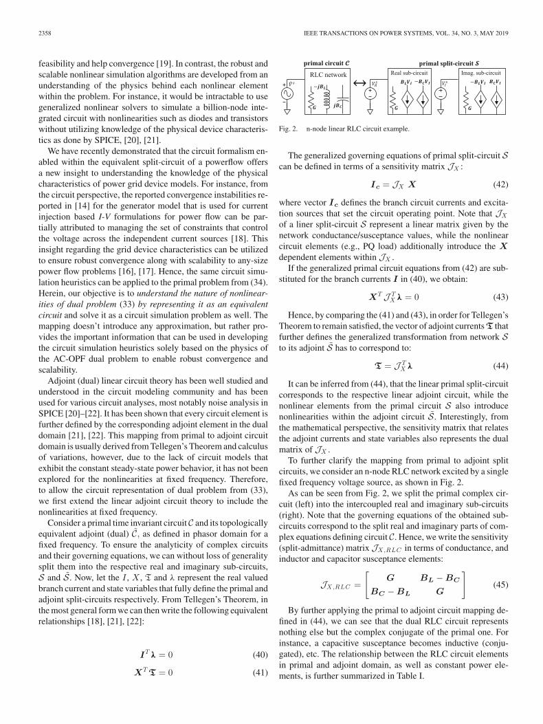
To further clarify the mapping from primal to adjoint splitcircuits, we consider an n-node RLC network excited by a singlefixed frequency voltage source, as shown in Fig. 2.
As can be seen from Fig. 2, we split the primal complex cir-cuit (left) into the intercoupled real and imaginary sub-circuits(right). Note that the governing equations of the obtained sub-circuits correspond to the split real and imaginary parts of com-plex equations defining circuit C. Hence, we write the sensitivity(split-admittance) matrix JX,RLC in terms of conductance, andinductor and capacitor susceptance elements:
JX,RLC =
[G BL − BC
BC − BL G
](45)
By further applying the primal to adjoint circuit mapping de-fined in (44), we can see that the dual RLC circuit representsnothing else but the complex conjugate of the primal one. Forinstance, a capacitive susceptance becomes inductive (conju-gated), etc. The relationship between the RLC circuit elementsin primal and adjoint domain, as well as constant power ele-ments, is further summarized in Table I.
JEREMINOV et al.: EQUIVALENT CIRCUIT FORMULATION FOR SOLVING AC OPTIMAL POWER FLOW 2359
TABLE IMAPPING OF CIRCUIT ELEMENTS TO DUAL DOMAIN
To analyze the mapping and effect of excitation sources tothe adjoint network, we first consider the excitation sourcesof primal split-circuit S. As it was shown in [21], [22], thesensitivities of excitation sources that set the operating point ofthe primal circuit S are zero (e.g., constant current and voltagesource), and hence do not affect the adjoint circuit. Therefore,the primal excitation sources in the adjoint circuit are turnedOFF, as presented in Table I. To further understand and analyzethe effect of adding the excitation to the adjoint circuit, let ψc
represent the vector of adjoint excitation sources. We can thenreformulate the expression from (44) as:
J TX λ = ψc (46)
Next, by comparing the generalized adjoint circuit equationsfrom (46) with the dual problem form the optimality KKT con-ditions given in (33), we recognize that the vector of adjointexcitation sources correspond to the negative gradient of the op-timization problem, in addition to the contributions of the dualvariables related to the inequality constraints. Therefore, fromthe circuit perspective, the negative gradient of the objectivefunction and the dual variables related to inequality constraintsrepresent the adjoint sources that set the operating point of theadjoint circuit in a manner that ensures controlled and optimizedprimal circuit operating point. For instance, consider again then-node RLC circuit from Fig. 2. Its adjoint circuit correspondsto the conjugated RLC network and shorted voltage sources(OFF). However, it can be shown that turning the adjoint excita-tion voltage sources ON ensures that the current supplied by theprimal voltage sources is minimized, thereby corresponding toadding the objective function of minimizing the voltage sourcecurrent to the optimization problem constrained by the RLCcircuit equations from Fig. 2.
With the relationship between the primal and dual problemsfrom (33), (34) and their equivalent circuit representation estab-lished, the set of complementary slackness conditions from (35)remain to be considered. Therefore, we introduce the optimiza-tion control circuits, whose governing equations are defined bythe complementary slackness conditions, which as discussedabove, further set the values of the adjoint (dual) variables rep-resenting the portion of adjoint excitation sources.
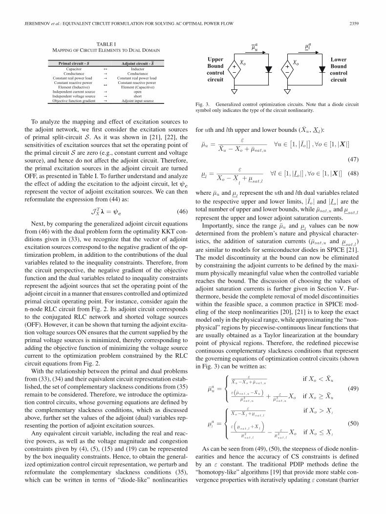
Any equivalent circuit variable, including the real and reac-tive powers, as well as the voltage magnitude and congestionconstraints given by (4), (5), (15) and (19) can be representedby the box inequality constraints. Hence, to obtain the general-ized optimization control circuit representation, we perturb andreformulate the complementary slackness conditions (35),which can be written in terms of “diode-like” nonlinearities
Fig. 3. Generalized control optimization circuits. Note that a diode circuitsymbol only indicates the type of the circuit nonlinearity.
for uth and lth upper and lower bounds (Xu , Xl):
μu =ε
Xu − Xo + μsat,u∀u ∈
[1,
∣∣Io
∣∣] ,∀o ∈ [1, |X|]
(47)
μl=
ε
Xo − X−l+ μ
sat,l
∀l ∈ [1, |Io |] ,∀o ∈ [1, |X|] (48)
where μu and μl
represent the uth and lth dual variables relatedto the respective upper and lower limits, |Io | and |Io | are thetotal number of upper and lower bounds, while μsat,u and μ
sat,l
represent the upper and lower adjoint saturation currents.Importantly, since the range μu and μ
lvalues can be now
determined from the problem’s nature and physical character-istics, the addition of saturation currents (μsat,u and μ
sat,l)
are similar to models for semiconductor diodes in SPICE [21].The model discontinuity at the bound can now be eliminatedby constraining the adjoint currents to be defined by the maxi-mum physically meaningful value when the controlled variablereaches the bound. The discussion of choosing the values ofadjoint saturation currents is further given in Section V. Fur-thermore, beside the complete removal of model discontinuitieswithin the feasible space, a common practice in SPICE mod-eling of the steep nonlinearities [20], [21] is to keep the exactmodel only in the physical range, while approximating the “non-physical” regions by piecewise-continuous linear functions thatare usually obtained as a Taylor linearization at the boundarypoint of physical regions. Therefore, the redefined piecewisecontinuous complementary slackness conditions that representthe governing equations of optimization control circuits (shownin Fig. 3) can be written as:
μau =
⎧⎪⎨⎪⎩
εXu −Xo + μs a t , u
if Xo < Xu
ε(μs a t , u −Xu )μ2
s a t , u+ ε
μ2s a t , u
Xo if Xo ≥ Xu
(49)
μ−al
=
⎧⎪⎪⎨⎪⎪⎩
εXo −X− l
+μ−s a t , lif Xo > X− l
ε
(μ−s a t , l
+X− l
)μ−
2s a t , l
− εμ−
2s a t , l
Xo if Xo ≤ X− l
(50)
As can be seen from (49), (50), the steepness of diode nonlin-earities and hence the accuracy of CS constraints is definedby an ε constant. The traditional PDIP methods define the“homotopy-like” algorithms [19] that provide more stable con-vergence properties with iteratively updating ε constant (barrier
2360 IEEE TRANSACTIONS ON POWER SYSTEMS, VOL. 34, NO. 3, MAY 2019
parameter) until it approaches a small number at the point ofconvergence. However, beside the increase of iteration countduring the homotopic stepping toward the original problem, thenonlinear constraint optimization problems cannot guaranteethe problem feasibility on the whole homotopy path [19]. Onthe other side, SPICE has developed the limiting and homotopyalgorithms [21] that efficiently handle the extremely steep non-linearities (e.g., diodes, transistor switches, etc.) within circuitsof enormous scale and complexity. Therefore, instead of ap-plying the traditional PDIP algorithms to handle the steepnessof the “diode-like” curves, we keep (49), (50) steep from thebeginning of simulation, and modify the SPICE-style heuristics[21] to develop the Critical Curvature Region for limiting. Thisis discussed in further detail in Section V.
Lastly, after we showed that the complete optimization prob-lem defined by the equivalent circuit constraints can be repre-sented in terms of equivalent circuits and solved as an equivalentcircuit problem, we define the Equivalent Circuit Programmingas a new class of optimization problems.
Definition 1: (Equivalent Circuit Program - ECP). An opti-mization problem whose constraints can be expressed in termsof equivalent circuit equations. Therefore, the problem optimal-ity conditions represent the governing equations of an equiva-lent circuit, whose operating point can be obtained by solving acircuit simulation problem. Most importantly, if sufficient con-ditions are met, the ECP operating point exactly represent anoptimal solution of the optimization problem.
1) Generic Framework for Optimizing Power Grid: Anequivalent split-circuit formulation was demonstrated to pro-vide a generalized power system simulation framework [15]–[17], [23]–[27] that can include any physics-based model, suchas induction motors [24] or power electronics [23]. Since bothtransmission and distribution networks can be represented by anequivalent circuit, they can be simulated (jointly [26] or sepa-rately [25]) within the same framework. Furthermore, the circuitsimulation modeling methodology used in modeling the steeplynonlinear devices, such as transistor switches, can be adapted[27] to develop the continuous models of nonlinear power griddevice characteristics. This includes PV/PQ conversion of thegenerators and shunts, as well as the transformer tap control[27]. Most importantly, the globally convergent heuristics thatare relied upon in SPICE can be adapted to ensure the robustconvergence properties of the developed nonlinear models [21],[27].
Lastly, since each of the split-circuit models are further de-fined within the adjoint domain, the proposed framework formodeling and solving the optimal power flow problem can begeneralized to incorporate any physics-based models. For theAC-OPF problem specifically, we derive the ECP model of agenerator that contains the embedded objective function gradi-ent within the model. This further ensures the minimized gen-erated real power solution.
2) AC-OPF Circuit Model of a Generator: The complexgoverning equations of a generator model and the respectivereal and reactive power constraints are given in (10) and (15),(16). The powerflow circuit for the generator in terms of admit-tance state variables is derived by splitting (10) into its real and
Fig. 4. Powerflow equivalent circuit of a generator.
imaginary currents IGR,g and IGI ,g :
IGR,g = GG,gVR,Γ − BG,gVI ,Γ ∀g ∈ G (51)
IGI ,g = GG,gVI ,Γ + BG,gVR,Γ ∀g ∈ G (52)
Moreover, the real and reactive power constraints are repre-sented by the two additional equivalent circuits as in Fig. 4,where the powers are proportional to the currents flowingthrough the voltage source set by the bus voltage magnitude.
We start the derivation of adjoint power flow circuit by findingthe first order sensitivity Jg (X) matrix of the GB generatorgoverning equations that satisfies (42):
To further set the operating point of the adjoint power flow cir-cuit that ensures that the real power supplied by the generator isminimized as well as bounded by the power control circuits, thegoverning equations of generator adjoint circuit can be writtenfrom established relationships in (33) and (46) as:
where λR,Γ and λI ,Γ represent the adjoint voltages, μP,g ,μ
P,g, μQ,g and μ
Q,gare the dual variables related to upper and
lower bounds of real and reactive powers respectively, whileλP,g and λQ,g are the LMPs related to real and reactive powers.
The first two equations from (54) represent the main adjointsplit-circuit governing equations of a generator. By letting thereal and imaginary adjoint currents (�GR,g and �GI ,g ) be afunction of currents at the generator output terminal, we furtherwrite the nonlinear adjoint split-circuit currents of a generator:
�GR,g = GG,gλR,Γ + BG,gλI ,Γ ∀g ∈ G (55)
�GI ,g = GG,gλI ,Γ − BG,gλR,Γ ∀g ∈ G (56)
Note that the currents from (55), (56) define the adjoint ad-mittance of the generator GB model, as shown by Table I. Most
JEREMINOV et al.: EQUIVALENT CIRCUIT FORMULATION FOR SOLVING AC OPTIMAL POWER FLOW 2361
Fig. 5. Adjoint powerflow circuit of a generator that supplies optimal realpower, enforced by embedded to objective function gradient to G-Circuit.
importantly, the use of power flow and adjoint generator cur-rents is the typical practice in equivalent circuit modeling. Therespective currents are not the variables of the formulation,but rather an aggregation of the rest of the system, for whichgoverning equations are built by hierarchically combining therespective circuit models of the simulation problem.
The next four equations from (54) are given as:
VR,ΓλR,Γ + VI ,ΓλI ,Γ + dsq,ΓλP,g = 0 ∀g ∈ G (57)
VR,ΓλI ,Γ − VI ,ΓλR,Γ − dsq,ΓλQ,g = 0 ∀g ∈ G (58)
λP,g = μP,g
− bg − 2cgPG,g − μP,g ∀g ∈ G (59)
λQ,g = μQ,g
− μQ,g ∀g ∈ G (60)
To further reduce the variable count of the AC-OPF circuit,we can eliminate the Lagrange multipliers related to the real andreactive powers (λP,g and λQ,g ) by substituting (59), (60) into(57), (58) respectively. This which further yields the constraintsadded to ensure the optimality and control of the powers suppliedby the conductance and susceptance state variables, governingthe G-circuit and B-circuit from Fig. 5. The nonlinear adjointpowerflow circuit of a generator that maps (55), (56) and (57)–(60) is shown in Fig. 5.
It is important to note that the derived governing circuit equa-tions precisely represent the part of KKT conditions contributedto the generator modeling constraints. Hence, to solve the non-linear circuit simulation problem, each of the nonlinear primaland adjoint circuit equations are linearized by means of thefirst order Taylor expansion [15]–[17] to obtain the linearizedECP circuit models that are then combined together to build tocomplete ECP representation of AC-OPF problem.
3) Building and Solving an Equivalent Circuit Program:The complete ECP circuit representation is obtained by hi-erarchically combining (connecting) the primal, adjoint andcontrol circuit models, as defined by the grid (network) topol-ogy. It is important to note that the hierarchical building of thecircuit representation corresponds to a modular construction ofthe Jacobian/Hessian matrix and constant vector that defines theNewton Raphson values during the iteration process.
Once the complete equivalent split-circuit is built, its set ofgoverning circuit equations correspond to the nonlinear set ofKKT optimality conditions as linearized by a first order Taylorexpansion. This linearization represents that step for the inner
most loop of the Newton Raphson method. Since iterativelysolving the circuit simulation problem corresponds to NewtonRaphson iterations, at every iteration only circuit elements (Ja-cobian/Hessian terms) that are dependent on the values fromthe previous iteration are rebuilt, while the linear parts are builtonce at the beginning of the simulation. This approach wasshown to represent an extremely efficient formulation and so-lution method for solving nonlinear circuit problems [18], [21].The main difference between the circuit simulation and tradi-tional methods, however, is the circuit formalism obtained fromthe circuit representation of the problem. This provides impor-tant information that allows for developing efficient heuristicsto ensure the robust convergence properties and scalability di-rectly from the physical characteristics of the problem, as furtherdiscussed in the following section.
V. ENHANCED SIMULATION OF CIRCUIT-BASED AC-OPFPROBLEM EQUIVALENT (ESCAPE) APPROACH
Solving the nonlinear constrained optimization (NCO) prob-lem can be a very challenging task that is prone to divergenceor very slow convergence. These challenges can arise due tothe inefficient handling of nonlinear constraints combined withmodeling of inequality constraints. One of the widely used meth-ods for solving the NCO problems, Primal Dual Interior Point(PDIP) method [19], tackles those challenges by multiplying theentire solution vector with the smallest damping factor neededto maintain the iteration as feasible and further decrease theerror. However, since the first introduction of the SPICE-likesimulators [20], it has been shown that damping the completesolution vector of a nonlinear simulation has two serious draw-backs [20]. First, if the iterative solutions are in vicinity ofthe correct solution, the convergence process is unnecessarilyslowed down. Second, if the solutions of two consecutive it-erations differ widely, the problem may diverge or oscillate.Importantly, from the perspective of optimization problem, theunnecessary damping of certain variables from a complete so-lution vector can force the iteration process to remain stuck inthe local area, hence increases the chances of converging to alocal solution or a saddle point. Therefore, instead of applyingthe traditional PDIP algorithms to solve the AC-OPF circuit,we use the idea of modeling the complementary slackness con-ditions as in PDIP and combine it with a circuit simulationsolution approach to the problem to derive a new simulationtechnique.
Herein, we introduce our Enhanced Simulation of Circuit-based AC-OPF Problem Equivalent (ESCAPE) approach as anadaptation of limiting heuristics from circuit simulations.
A limiting technique can be generalized as follows: for a givenmaximum step size vector ΔΥmax , we can find the vector ofdamping factors (δC) that limits the NR variable update as:
δC = min {e, [sign (ΔΥ) � ΔΥmax ] � ΔΥ} (61)
Υk+1 = Υk + δC � ΔΥ (62)
where � represent the pointwise division, e is a vector of ones,and Υ is a placeholder vector of limited variables. Note from
2362 IEEE TRANSACTIONS ON POWER SYSTEMS, VOL. 34, NO. 3, MAY 2019
(61) that in contrast to the traditional damping approaches, eachof the variables herein can have its own limiting factor.
A. Voltage Limiting
Voltage Limiting was shown be a simple and effective sim-ulation technique that limits the value of the step change thatthe real and imaginary voltage vectors are allowed to make dur-ing each NR iteration in powerflow problem [16], [17]. For theAC-OPF circuit, the voltage limiting is done in two stages. Inthe first one, we limit the powerflow real and imaginary volt-age steps, i.e., Υ ∈ {V R,V I} as in (61) and use the obtaineddamping vectors to limit the real and imaginary adjoint volt-ages respectively. To further ensure that the step sizes of adjointvoltages do not exceed the predefined limits, the second stageapplies limiting technique to adjoint voltages.
B. Admittance Limiting
As discussed in [16], the voltages of powerflow equivalentcircuit are very sensitive to the reactive power change duringnonlinear iteration. Hence, we redefine the Q limiting [16], [17]to limit the NR step change of the admittance state variablesof the generator model. With well-defined bounds on admit-tance state variables from the bounds on real and reactive powerand voltage magnitude, we establish the maximum step changevectors for the generator conductance and susceptance:
ΔGmax = α (Gmax − Gmin ) (63)
ΔBmax = α (Bmax − Bmin ) (64)
where α ∈ (0, 1] represent the discretizing factor.
C. Critical Curvature Region (CCR) Limiting
In contrast to the feasible range of the power flow split-circuitvariables that are normalized and well defined by the bounds ofthe optimization problem, the set of adjoint variables, partic-ularly the ones related to problem bounds, may not be wellbounded in general. However, as shown in Section III, the gra-dient of the objective function represents an excitation source ofthe adjoint circuit, and thereby determines its operating point.Therefore, in order to prevent the large variations of dual vari-ables, the first step in obtaining the efficient limiting heuristicsis normalizing the adjoint circuit.
1) Normalizing the Adjoint Circuit: Consider a quadraticcost function from (1) that is defined by the set of cost func-tion coefficients {a, b, c}. Herein, we introduce the adjoint perunit normalization (a.p.u.) of the adjoint excitation sources; i.e.,gradient of the objective function (Section III). Importantly,since scaling of the cost function by a positive constant doesn’taffect its minima, we obtain the base-factor that normalizes theobjective function as:
bapu = max [max (b, 2c)] (65)
The normalized objective function now sets the adjoint cir-cuit operating point in the range of around 1 a.p.u. Therefore,the values of dual variables set by the upper and lower bound
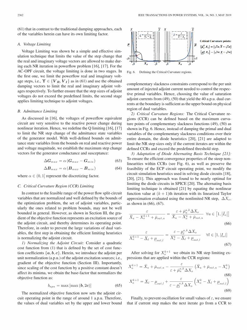
Fig. 6. Defining the Critical Curvature regions.
complementary slackness constraints correspond to the per unitamount of injected adjoint current needed to control the respec-tive primal variables. Hence, choosing the value of saturationadjoint currents from (49), (50) that yield the 40 a.p.u. dual cur-rents at the boundary is sufficient as the upper bound on physicalregion of dual variables.
2) Critical Curvature Regions: The Critical Curvature re-gions (CCR) can be defined based on the maximum curva-ture points of complementary slackness functions (49), (50) asshown in Fig. 6. Hence, instead of damping the primal and dualvariables of the complementary slackness conditions over theirentire domain, the diode heuristics [20], [21] are adapted tolimit the NR step sizes only if the current iterates are within thedefined CCRs and exceed the predefined threshold step.
3) Adaptation of Diode Alternating Basis Technique [21]:To ensure the efficient convergence properties of the steep non-linearities within CCRs (see Fig. 6), as well as preserve thefeasibility of the ECP circuit operating point, we modify thecircuit simulation heuristics used in solving diode circuits [18],[20], [21]. This approach was found to be nearly optimal forlimiting the diode circuits in SPICE [20]. The alternating basislimiting technique is obtained [21] by equating the nonlinearfunction value at (k + 1)th iteration with its linearized Taylorapproximation evaluated using the nonlimited NR step, ΔXo,as shown in (66), (67).
ε
Xu − Xk+1o + μsat,u
=ε + μa,k
u ΔXo
Xu − Xko + μsat,u
∀u ∈[1,
∣∣Io
∣∣](66)
ε
Xk+1o − Xl + μ
sat,l
=ε − μa,k
lΔXo
Xko − Xl + μ
sat,l
∀l ∈ [1, |Io |]
(67)
After solving for Xk+1o we obtain its NR step limiting ex-
pressions that are applied within the CCR regions:
Xk+1o = Xu + μsat,u − ε
ε + μa,ku ΔXo
(Xu + μsat,u − Xk
o
)(68)
Xk+1o = Xl − μ
sat,l+
ε
ε − μa,kl ΔXo
(Xk
o − Xl + μsat,l
)(69)
Finally, to prevent oscillation for small values of ε, we ensurethat if current step makes the next iterate go from a CCR to
JEREMINOV et al.: EQUIVALENT CIRCUIT FORMULATION FOR SOLVING AC OPTIMAL POWER FLOW 2363
neutral region or vice versa, we limit it such that it has to stopat the maximum curvature point before entering a new region.
D. Embedding the Homotopy Within the ECP Circuit
To allow the robust convergence of any large-scale powersystem optimization problem, we extend the Tx-stepping ho-motopy method [16], [27] to the adjoint domain. The solutionof the optimal power flow is obtained by embedding the homo-topy factor η ∈ [0, 1] to linear series and shunt network elementsand transformer model, as shown in (70)–(72). The system equa-tions are then sequentially solved via the relaxed ECP problemswhile gradually decreasing the homotopy factor to zero fromone. Namely, for the initial homotopy factor set to one, the ECPcircuit is virtually “shorted.” Now, the optimal power flow solu-tion corresponds to the economic dispatch solution and can betrivially obtained under the assumption that there is sufficientgeneration in the system to supply the load. Gradually decreas-ing the embedded homotopy factor η to zero sequentially relaxesthe ECP circuit toward its original state, while using the solutionfrom the previous sub-problem to initialize the ECP circuit forthe next homotopy decrement:
GL + jBL = (ηΥ + 1) (GL + jBL ) (70)
t (η) = t + (1 − t) η (71)
θph (η) = (1 − η) θph (72)
where Υ represents an admittance scaling factor, t is the trans-former tap, and θph is the phase shifting angle.
E. Towards a Globally Convergent AC-OPF Algorithm
Years of research in the circuit simulation field have advancedthe techniques of Newton Raphson step limiting and applica-tion of homotopy methods that are shown to exhibit globalconvergence properties [18], [21]. We have shown that the sameheuristics can be adapted and extended to the power systemsimulation problems, thereby guaranteeing similar global con-vergence properties [17], [26], [27]. Furthermore, by strictlyremoving the discontinuities of the complementary slacknessconditions (49), (50) and with extension of the power flowheuristic and homotopy algorithms to the adjoint (dual) do-main, it can be demonstrated that if a feasible solution doesexist, the circuit simulation techniques can bound the NR stepwhile maintaining the full rank solution matrix throughout thesimulation [27]. It follows that the same robust convergenceproperties remain within the ECP problems, such as AC-OPF.
VI. SIMULATION RESULTS
The circuit element library for the derived models that mapthe AC-OPF problem was built and incorporated in MATLAB toimplement the ESCAPE algorithm. The tool reads in the ‘mpc’input file, translates the parsed information into the circuit pa-rameters, hierarchically builds the sparse circuit equations bycombining the circuit models that correspond to building theset of KKT conditions, and then iteratively solves them tofind the operating point of the AC-OPF circuit. In addition
to the nonlinear circuit simulator, a linear simulator is usedto initialize the adjoint split-circuit. All the simulations wererun on MacBook Pro 2.9 GHz Intel Core i7.
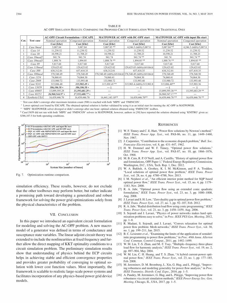
We demonstrate the robustness of our circuit formulationbased approach by evaluating the following: 1) IEEE pglib andPEGASE test cases libraries; 2) local optimal solutions testcases from [5]; 3) GridPack data set library from PNLL; and4) Synthetic Eastern Interconnection test case [29]. The prob-lems were initialized using the real power and the voltage angleobtained from a DC-OPF solution that includes a flat startfor voltage magnitudes and reactive powers given by the meanvalues defined by respective limits. Each of the test cases issolved for current congested (upper bound on maximum currentmagnitude of transmission line) and nominal operating condi-tions (without congestion constraints). We compare the resultsfor our ECP formulation with the ‘PQV’AC-OPF and relaxed‘SDP’ AC-OPF formulations solved with ‘MIPS’/’FMINCON’and ‘SDPT3’ toolboxes by using the default input solver param-eters, (maximum constraint violation 5E-6, optimality tolerance1E-4, variable tolerance of 1E-4 p.u. and a maximum iterationcount of 500 iterations) within the MATPOWER solver. Theresults are summarized in Table II.
The ESCAPE technique obtained a solution for all of theexamined test cases during both operating conditions and con-verged to the same optimal solution point for each case (Table II)starting from both DC-OPF and input file initial starts. In con-trast, the MATPOWER ‘MIPS’ solver failed on several of thetestcases, notably the larger size systems, and the ‘FMINCON’toolbox performed better in those cases, but also diverged forthe two smaller cases when initialized from DC-OPF. For thisreason, we present the MATPOWER results as initialized fromDC-OPF and test case input file separately. Lastly, the SDP re-laxation performed as reported in the literature [5], [12], and itwas characterized by slower runtimes than the other approaches.Furthermore, the SDP relaxation failed to converge for the testcases that are known to have multiple local solutions and wasable to successfully find the global solutions of the 14, 30 and 89bus test cases that match the solutions obtained from ESCAPEand MATPOWER.
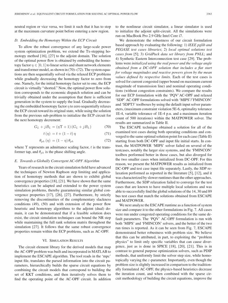
We next analyze the ESCAPE runtime as a function of systemsize and compare it to the other formulations in Fig. 7. All caseswere run under congested operating conditions for the same de-fault parameters. The ‘PQV’ AC-OPF formulation is run withboth ‘MIPS’ and ‘FMINCON’ solvers, and the better of the tworun times is reported. As it can be seen from Fig. 7, ESCAPEdemonstrated better robustness with problem size. We believethat this can be attributed, in part, to exploiting the “problemphysics” to limit only specific variables that can cause diver-gence, just as is done in SPICE [18], [20], [21]. This is incontrast to general purpose optimization solvers, such as PDIPmethods, that uniformly limit the solver step size, while homo-topically varying the ε-parameter. Importantly, even though theproblem size is slightly increased in comparison to the tradition-ally formulated AC-OPF, the physics-based heuristics decreasethe iteration count, and when combined with the sparse cir-cuit methodology of building the circuit equations, improve the
2364 IEEE TRANSACTIONS ON POWER SYSTEMS, VOL. 34, NO. 3, MAY 2019
TABLE IIAC-OPF SIMULATION RESULTS: COMPARING THE PROPOSED CIRCUIT FORMULATION WITH THE TRADITIONAL ONES
— Test case didn’t converge after maximum iteration count (500) is reached with both ‘MIPS’ and ‘FMINCON’.� Lower optimal cost found by ESCAPE. The obtained optimal solution is further validated by using it as an initial start for running the AC-OPF in MATPOWER.∗∗ ‘MIPS’ MATPOWER solver diverged or didn’t converge after one hour; optimal solution obtained using ‘FMINCON’ toolbox.§ Case13659 did not run with both ‘MIPS’ and ‘FMINCON’ solvers in MATPOWER, however, authors in [30] have reported the solution obtained using ‘KNITRO’ given as:$386,107.5 for both operating conditions.
Fig. 7. Optimization runtime comparison.
simulation efficiency. These results, however, do not excludethat the other toolboxes may perform better, but rather indicatea promising path toward developing a generalized and robustframework for solving the power grid optimizations solely fromthe physical characteristics of the problem.
VII. CONCLUSION
In this paper we introduced an equivalent circuit formulationfor modeling and solving the AC-OPF problem. A new macro-model of a generator was defined in terms of conductance andsusceptance state variables. The linear adjoint circuit theory wasextended to include the nonlinearities at fixed frequency and fur-ther allow the direct mapping of KKT optimality conditions to acircuit simulation problem. The preliminary simulation resultsshow that understanding of physics behind the ECP circuitshelps in achieving stable and efficient convergence propertiesand provides greater probability of converging to optimal so-lution with lower cost function values. Most importantly, theframework is scalable to realistic large-scale power systems andfacilitates incorporation of any physics-based power grid devicemodels.
REFERENCES
[1] W. F. Tinney and C. E. Hart, “Power flow solutions by Newton’s method,”IEEE Trans. Power App. Syst., vol. PAS-86, no. 11, pp. 1449–1460,Nov. 1967.
[2] J. Carpentier, “Contribution to the economic dispatch problem,” Bull. Soc.Francaise Electriciens, vol. 8, pp. 431–447, 1962.
[3] H. W. Dommel and W. F. Tinney, “Optimal power flow solutions,”IEEE Trans. Power App. Syst., vol. PAS-87, no. 10, pp. 1866–1876,Oct. 1968.
[4] M. B. Cain, R. P. O’Neill, and A. Castillo, “History of optimal power flowand formulations, OPF Paper 1,” Federal Energy Regulatory Commission,Washington, D.C., USA, Tech. Rep. 1, Dec. 2012.
[5] W. A. Bukhsh, A. Grothey, K. I. M. McKinnon, and P. A. Trodden,“Local solutions of optimal power flow problem,” IEEE Trans. PowerSyst., vol. 28, no. 4, pp. 4780–4788, Nov. 2013.
[6] I. M. Nejdawi et al., “An efficient interior point method for SQP basedoptimal power flow,” IEEE Trans. Power Syst., vol. 15, no. 4, pp. 1179–1183, Nov. 2000.
[7] R. A. Jabr, “Optimal power flow using an extended conic quadraticformulation,” IEEE Trans. Power Syst., vol. 23, no. 3, pp. 1000–1008,Aug. 2008.
[8] J. Lavaei and S. H. Low, “Zero duality gap in optimal power flow problem,”IEEE Trans. Power Syst., vol. 27, no. 1, pp. 92–107, Feb. 2012.
[9] R. A. Jabr, “Radial distribution load flow using conic programming,” IEEETrans. Power Syst., vol. 21, no. 3, pp. 1458–1459, Aug. 2006.
[10] S. Sojoudi and J. Lavaei, “Physics of power networks makes hard opti-mization problems easy to solve,” in Proc. IEEE PES Gen. Meeting, 2012,pp. 1–8.
[11] R. Madani, S. Sojoudi, and J. Lavaei, “Convex relaxation for optimalpower flow problem: Mesh networks,” IEEE Trans. Power Syst., vol. 30,no. 1, pp. 199–211, Jan. 2015.
[12] B. C. Lesieutre et al., “Examining the limits of the application of semidef-inite programming to power flow problems,” in Proc. 49th Annu. AllertonConf. Commun. Control Comput., 2011, pp. 1492–1499.
[13] W. M. Lin, T.-S. Zhan, and M.-T. Tsay, “Multiple–frequency three-phaseload flow for harmonic analysis,” IEEE Trans. Power Syst., vol. 19, no. 2,pp. 897–904, May 2004.
[14] W. M. Lin, C. H. Huang, and T. S. Zhan, “A hybrid current-power opti-mal power flow,” IEEE Trans. Power Syst., vol. 23, no. 1, pp. 177–185,Feb. 2008.
[15] M. Jereminov, D. M. Bromberg, L. Xin, G. Hug, and L. Pileggi, “Improv-ing robustness and modeling generality for power flow analysis,” in Proc.IEEE Transmiss. Distrib. Conf. Expo., 2016, pp. 1–5.
[16] A. Pandey, M. Jereminov, G. Hug, and L. Pileggi, “Improving power flowrobustness via circuit simulation methods,” IEEE Power Energy Soc. Gen.Meeting, Chicago, IL, USA, 2017, pp. 1–5.
JEREMINOV et al.: EQUIVALENT CIRCUIT FORMULATION FOR SOLVING AC OPTIMAL POWER FLOW 2365
[17] A. Pandey, M. Jereminov, M. Wagner, G. Hug, and L. Pileggi, “Robustconvergence of power flow using T-x stepping method with equivalentcircuit formulation,” in Proc. Power Syst. Comput. Conf., Dublin, Ireland,2018, pp. 1–7.
[18] L. Pileggi, R. Rohrer, and C. Visweswariah, Electronic Circuit & SystemSimulation Methods. New York, NY, USA: McGraw-Hill, 1995.
[19] S. Boyd and L. Vandenberghe, Convex Optimization. New York, NY, USA:Cambridge Univ. Press, 2004.
[20] L. Nagel and R. Rohrer, “Computer analysis of nonlinear circuits, exclud-ing radiation (CANCER),” IEEE J. Solid-State Circuits, vol. SSC-6, no. 4,pp. 166–182, Aug. 1971.
[21] W. J. McCalla, Fundamentals of Computer-Aided Circuit Simulation.Boston, MA, USA: Kluwer, 1988.
[22] S. W. Director and R. Rohrer, “The generalized adjoint network andnetwork sensitivities,” IEEE Trans. Circuit Theory, vol. 16, no. 3, pp. 318–323, Aug. 1969.
[23] M. Jereminov, A. Pandey, D. M. Bromberg, X. Li, G. Hug, and L. Pileggi,“Steady-state analysis of power system harmonics using equivalent split-circuit models,” in Proc. Innov. Smart Grid Technol. Conf. Eur., Ljubljana,Slovenia, Oct. 2016, pp. 1–6.
[24] A. Pandey, M. Jereminov, X. Li, G. Hug, and L. Pileggi, “Unified powersystem analyses and models using equivalent circuit formulation,” in Proc.IEEE Power Energy Soc. Innov. Smart Grid Technol., Minneapolis, St.Paul, USA, 2016, pp. 1–5.
[25] M. Jereminov, D. M. Bromberg, A. Pandey, X. Li, G. Hug, and L. Pileggi,“An equivalent circuit formulation for three-phase power flow analysisof distribution systems,” in Proc. IEEE Transmiss. Distrib. Conf. Expo.,Dallas, TX, USA, 2016, pp. 1–5.
[26] A. Pandey, M. Jereminov, M. Wagner, D. M. Bromberg, G. Hug, andL. Pileggi, “Robust power flow and three phase power flow analyses,”IEEE Trans. Power Syst., vol. 34, no. 1, pp. 616–626, Jan. 2019, doi:10.1109/TPWRS.2018.2863042.
[27] A. Pandey, “Robust steady-state analysis of power grid using equiva-lent circuit formulation with circuit simulation methods,” Doctoral thesis,Dept. Elect. Comput. Eng., Carnegie Mellon Univ., Pittsburgh, PA, USA,Aug. 2018.
[28] D. K. Molzahn and L. A. Roald, “Towards an AC optimal powerflow algorithm with robust feasibility guarantees,” in Proc. Power Syst.Comput. Conf., 2018, pp. 1–7. [Online]. Available: https://molzahn.github.io/pubs/molzahn_roald-acopf_robust2018.pdf
[29] A. B. Birchfield, T. Xu, and T. Overbye, “Power flow convergence andreactive power planning in creation of large synthetic grids,” IEEE Trans.Power Syst., vol. 33, no. 6, pp. 6667–6674, Nov. 2018.
[30] C. Josz et al., “AC power flow data in MATPOWER and QCQP format:iTesla RTE snapshots and PEGASE,” ArXiv, 1603.01533, Mar. 2016.
Marko Jereminov (M’15) was born in Belgrade,Serbia. He received the B.Sc. degree in electricalengineering from South Carolina State University,South Carolina, USA, in 2016, and is currently work-ing toward the Ph.D. degree in electrical and com-puter engineering at Carnegie Mellon University,Pittsburgh, PA. He previously interned at Pearl StreetTechnologies, Pittsburgh, as well as at the Departmentof Electrical and Computer Engineering, CarnegieMellon University, prior to joining as a Ph.D. student.His research interests include optimization, simula-
tion, and modeling of electrical power systems.
Amritanshu Pandey was born in Jabalpur, India.He received the M.Sc. degree in electrical engineer-ing from Carnegie Mellon University, Pittsburgh, PA,in 2012, where he is currently working toward thePh.D. degree. Prior to joining as a doctoral student atCarnegie Mellon University, he was an Electrical En-gineer with MPR Associates, Inc., from 2012 to 2015.He has previously interned at Pearl Street Technolo-gies, ISO New-England and GE Global Research. Hisresearch interests include modeling and simulation,optimization and control of power systems.
Larry Pileggi (F’02) received the Ph.D. degree inelectrical and computer engineering from CarnegieMellon University in 1989. He is the Tanoto Professorof electrical and computer engineering with CarnegieMellon University, and has previously held positionsat the Westinghouse Research and Development andthe University of Texas at Austin. He has consultedfor various semiconductor and EDA companies, andwas the Co-founder of Fabbrix, Inc., Extreme DA,and Pearl Street Technologies. He is a Co-Author ofElectronic Circuit and System Simulation Methods
(McGraw-Hill, 1995) and IC Interconnect Analysis (Kluwer, 2002). He has au-thored or coauthored more than 300 conference and journal papers and holds 40U.S. patents. His research interests include various aspects of digital and analogintegrated circuit design and design methodologies, and simulation and mod-eling of electric power systems. Dr. Pileggi was a recipient of various awards,including Westinghouse Corporation’s highest engineering achievement award,the 2010 IEEE Circuits and Systems Society Mac Van Valkenburg Award, andthe 2015 Semiconductor Industry Association University Researcher Award.